the space of feasible solutions in metabolic networks
TRANSCRIPT

Journal of Physics Conference Series
OPEN ACCESS
The space of feasible solutions in metabolicnetworksTo cite this article A Braunstein et al 2008 J Phys Conf Ser 95 012017
View the article online for updates and enhancements
You may also likeHamiltonian analysis of 4-dimensionalspacetime in Bondi-like coordinatesChao-Guang Huang Shi-Bei Kong et al
-
Optimal solution of engineering designproblems through differential gradientevolution plus algorithm a hybridapproachMuhammad Farhan Tabassum Ali AkguumllSana Akram et al
-
Canonical simplicial gravityBianca Dittrich and Philipp A Houmlhn
-
This content was downloaded from IP address 10987184212 on 18022022 at 1743
The space of feasible solutions in metabolic networks
A Braunstein12 R Mulet3 A Pagnani11 Institute for Scientific Interchange Viale S Severo 65 I-10133 Torino Italy2 Politecnico di Torino Corso Duca degli Abruzzi I-10129 Torino Italy3 ldquoHenri-Poincare-Grouprdquo of Complex Systems and Department of Theoretical PhysicsPhysics Faculty University of Havana La Habana CP 10400 Cuba
E-mail pagnaniisiit
Abstract In this work we propose a novel algorithmic strategy that allows for an efficientcharacterization of the whole set of stable fluxes compatible with the metabolic constraints Thealgorithm based on the well-known Bethe approximation allows the computation in polynomialtime of the volume of a non full-dimensional convex polytope in high dimensions The resultof our algorithm match closely the prediction of Monte Carlo based estimations of the fluxdistributions of the Red Blood Cell metabolic network but in incomparably shorter time We alsoanalyze the statistical properties of the average fluxes of the reactions in the E-Coli metabolicnetwork and finally to test the effect of flux knock-outs on the size of the solution space of theE-Coli central metabolism
1 IntroductionCellular metabolism can be viewed as a chemical engine that transforms available raw materialsinto energy or into the building blocks needed for the biological function of the cells Althoughthe general topological properties of these networks are well characterized [1 2 3] and non-trivialpathways are well known for many species [4] the cooperative role of these pathways is hard tocomprehend Given the large size of these networks usually containing hundreds of metabolitesparticipating in an even larger number of reactions the comprehension of the principles thatgovern their global function turns out to be a real challenge A necessary step to deepen thecomprehension of metabolism at organism-wide level is the development of mathematical modelsand novel statistical techniques
It is well known that under evolutionary pressure prokaryotes cells like E-Coli behaveoptimizing their growth performance [5] Flux Balance Analysis (FBA) provides a powerfultool to predict from the whole space of phenotypic states which one will these cells acquireIn few words one may say that FBA maximizes a linear function (usually the growth rate ofthe cell) subject to biochemical and thermodynamic constraints [6] On the other hand cellswith genetically engineered knockouts or bacterial strains that were not exposed to selectionpressure need not to optimize their growth Under more general situations it is not clear whatobjective function should be maximized therefore a tool to characterize the shape and volumeof the whole space of possible phenotypic solutions must be welcome
Unfortunately this characterization has remained an elusive task Some recent attemptsto go beyond FBA have been recently proposed In [7] the authors propose an algorithmfor studying the maximal growth rate achievable and in [8] a solvable model of metabolicnetwork is introduced however to the best of our knowledge all attempts to obtain a systemic
International Workshop on Statistical-Mechanical Informatics 2007 (IW-SMI 2007) IOP PublishingJournal of Physics Conference Series 95 (2008) 012017 doi1010881742-6596951012017
ccopy 2008 IOP Publishing Ltd 1
pyruvateacetyl-
coa
fattyacids
ATP
simple sugars
polysaccaridesfood
fats
proteins aminoacids
glycolysis
citric acidcycle
ATP ATPATP
O2
oxydativephosph H2O
waste
NH3
CO2
Figure 1 Schematic representation of cell metabolism
characterization of cell metabolism have been based so far on Monte Carlo sampling of thesteady-state flux space [9] Unfortunately this kind of sampling is computationally very hardand unsuitable for whole-organism metabolic networks To address this problem we proposean algorithm that may efficiently characterize the whole set of stable fluxes imposed by thestoichiometric constraints by using a message passing algorithmic technique borrowed from thefield of statistical physics and information theory [10] One of the main advantage of this methodis the possibility to establish the relevance of any given reaction flux in terms of the relevanceof its contribution to the volume of the solutions space This can be done by measuring therelative volumersquos variation after knocking-out sequentially any reaction flux the larger is therelative variation the higher is the relevance of the flux in the metabolism of the organism
This work is organized in the following way in section 2 we will introduce the chemical basesof metabolism then in section 3 we outline the mathematical model Section 4 is devoted to givesome basic notions on differential geometry about volume in embedded manifolds In section 5we outline the derivation of the message passing equations and finally in section 6 we reviewcritically our findings indicating some work in progress extensions of our work
2 Cell metabolismEvery cell is composed in large part essentially of Hydrogen (H) Carbon (C) Nitrogen (N)and Oxygen (O) Such elements basically account for almost 99 of the cellrsquos weight Alreadyat this very coarse grained level of description if one consider the relative abundance on theearthrsquos crust of such chemicals (eg H represents only the 2 of the composition of the earthrsquoscrust and more than 50 of a generic cell) one easily realizes that living organism display avery peculiar kind of chemistry The constitutive building blocks of cells are grouped into fourfamilies
bull Sugars the main energy source for moleculesbull Fatty acids the components of cell membranesbull Amino Acids they serve as subunits in the synthesis of proteinsbull Nucleotides they play a central part in energy transfer and are also subunits from which
the informational macromolecules RNA and DNA are made
As displayed schematically in figure 1 cellular metabolism is a rather complex three-stageprocessing system
(i) Digestion breakdown of large macromolecules Food is transformed in order to be processedat a finer chemical level
International Workshop on Statistical-Mechanical Informatics 2007 (IW-SMI 2007) IOP PublishingJournal of Physics Conference Series 95 (2008) 012017 doi1010881742-6596951012017
2
H
D
E
F
G
I
-a 0-c0e00h
0
A
B
C
νi
aA + cC rarr eE + hHνi
Che
mic
al c
ompo
unds
Figure 2 Stoichiometric matrix detail of an ideal aA + cC rarr eE + hH reaction with flux νi
(ii) Glycolysis breakdown of simple sugar subunits into pyruvate and acetil-CoA This stageis anaerobic (no oxygen is utilized) and accompanied with a limited production of ATP Itis interesting to note that such module is an evolutionary relict dating back at the earlystage of life where oxygen on earthrsquos atmosphere was almost absent
(iii) Aerobic Oxidation complete oxidation of acetyl-CoA to H2O and CO2 accompanied nowby production of large amounts of ATP This metabolic module appeared at an evolutionarylater stage when organisms could have fully profit from the abundance oxygen and turnedout to be much more efficient then glycolysis in terms of the production of energy (egATP ADP etc)
Cell metabolism is very efficient since concentration of chemicals is normally buffered againstmajor environmental changes Fine tuning of global metabolic functions are acted by feed-back regulatory loops that decide almost instantaneously for the increasing (decreasing) of theproduction of specific enzymes The control a few key enzymes cause large scale reorganizationof the metabolic activity The laws governing metabolic biochemical reactions are encodedin the stoichiometric matrix that specifies the fixed integer proportion in which all chemicalsparticipate in each reaction It is worth pointing out that such integer proportions are constantsin the sense that are not condition dependent ie function of the temperature pressure pHetc and universal since the very same stoichiometric coefficients appears in all cells displayingthat given reaction Each metabolite has a row in the stoichiometric matrix and each reaction isspecified by a given column A positive stoichiometric coefficient has a positive (negative) signif it is produced (consumed) as shown in figure 2 Let us finally resume the general relevantproperties about the nature of stoichiometric constraints
bull Universality stoichiometry depends only on the chemical reaction and is both organismenvironmental conditions independent
bull Sparsity the number of metabolites generally involved in a reaction are small with respectto the overall number of metabolites
3 The mathematical modelThe fundamental equation characterizing all functional states of a reconstructed biochemicalreaction network is a mass conservation law that imposes simple linear constraints between theincoming and outgoing fluxes at any chemical reaction
partρ
partt= i + S middot ν minus o (1)
International Workshop on Statistical-Mechanical Informatics 2007 (IW-SMI 2007) IOP PublishingJournal of Physics Conference Series 95 (2008) 012017 doi1010881742-6596951012017
3
where ρ is the vector of the M metabolite concentrations in the network i (o) is the input(output) vector of fluxes and ν are the reaction fluxes governed by the M timesN stoichiometriclinear operator S encoding the coefficient of the M mass balance constraints among the N fluxes
Extensive studies on metabolism of different organism have shown that as long as theenvironmental condition are kept constant the variation in the concentration of metabolitesis constant too Moreover in case of a change in the external control parameters the newsteady state of the organism is reached almost instantaneously This allows to neglect transienteffects and concentrate on the static properties of our system
S middot ν = ominus i equiv b (2)
where b is the net metabolite uptake by the cell Without loss of generality we can assume thatthe stoichiometric matrix S has full rows rank ie that rank(S) = M since linearly dependentequations can be easily identified and removed Knowing that the number of metabolites M islower than the number of fluxes N the subspace of solutions is a (N minusM)-dimensional manifoldembedded in the N -dimensional space of fluxes
A linear space such that of the solutions of equation 2 is characterized by the property thatany linear combination of solutions is still a solution However there are a limitations on thespace of possible fluxes
bull Lower bound All reactions are considered as irreversible (a reversible reaction can betaken into account introducing a new independent irreversible reaction with reversed signstoichiometry) so fluxes are positive
bull Upper bound Enzymatically driven reaction are capped by the concentration of thesubstrate as described in the Michaelis-Menten kinetic equation [11] so for each specificreaction flux νi there is a maximal allowed flux νmax
i Unfortunately the determinationof maximal values is often experimentally very difficult and it can vary substantially fromin-vitro and in-vivo conditions
These limitations are expressed by the following vectorial inequality
0 le ν le νmax (3)
in such a way that together equation 2 and equation 3 define the convex set of all the allowedtime-independent phenotypic states of a given metabolic network
4 Subdimensional volumesThe space of feasible solutions consistent with the equations 2 constitutes an affine space V sub RN
of dimension N minusM The set of inequalities 3 then defines a convex polytope Π sub V that fromthe metabolic point of view may be considered as the allowed configuration space for the cellstates With the scope of describing it we will be interested in computing the volume ofthis space and certain volumes of subspaces of it Although conceptually simple the notionof sub-dimensional volume like that of Π requires some new definitions Consider any linearparameterization φ RNminusM rarr V sub RN as displayed in figure 3 A popular choice for φ isfor instance the inverse of the so called lexicographical projection ie the projection over thefirst N minus M coordinates such that its restriction to V has an inverse Being φ linear the(N minusM)timesN Jacobian matrix λ is constant and coincides with the matrix of φ in the canonicalbases Denoting λ = det(λdaggerλ)
12 the Euclidean metric in RN induces a measure on V (which
does not depend on φ) intV
f(ν)dν equiv λ
intf(φ(u))du (4)
International Workshop on Statistical-Mechanical Informatics 2007 (IW-SMI 2007) IOP PublishingJournal of Physics Conference Series 95 (2008) 012017 doi1010881742-6596951012017
4
U = φminus1(Π)
RN
φ RNminusM rarr V sub RN
V
Π
RNminusM
ν1MAXν2MAX
ν3MAX
Figure 3 Left panel sketch of the theparameterization φ RNminusM rarr V sub RN The polytope Π is a subset of hyperplane V
Π
ν i=
ν
ν
Figure 4 Geometrical interpretation of themarginal probability distributions
allowing to compute the volume of our polytope
volV (Π) equivint
V1Π(ν)dν = λ
int1φminus1(Π)(u)du (5)
where 1Π (middot) is the indicator function of the set Π It is worth pointing out that given the linearstructure of the metabolic equations the determinant of the mapping is a (scalar) constantAt this point on may wonder why donrsquot we compute the volume using the right hand side ofequation 5 Let us consider the case where φ is the lexicographical projection over the first NminusMvariables In such a case the transform expresses the last M variables in terms of the first NminusM Unfortunately this makes the system dense in the sense that now the equations would containO(N) variables a condition that turns out to be highly undesirable for the message passingstrategy that we will introduce later in section 5
The problem of describing the polytope Π can formulated in a probabilistic framework Wedefine the probability density P as
P(ν) = volV (Π)minus11Π(ν) (6)
Marginal flux probabilities over a given set of fluxes are obtained by integrating out all remainingdegrees of freedom In particular we can define single flux marginal probability densities asintegrals on the affine subspace W = V cap νi = ν
Pi(νi) =int
WP(ν)
prodj 6=i
dνj =1ΠcapW (νi)
volW (Π capW )(7)
where the normalization term volW (ΠcapW ) is the (sub dimensional) volume of the intersectionbetween the polytope Π and the hyperplane νi = ν as displayed schematically in figure 4 wherethe marginal probability at point νi = ν is proportional to length of the blue segment which isthe intersection between the polytope Π and the plane νi = ν
5 Computing the volume by message passingAll exact algorithms for the computation of the volume of a polytope are based on the knowledgeof its vertices The vertex enumeration problem however is P -hard [12 13] Various algorithmsexist for calculating the exact volume of a polytope from its vertexes (for a review see [14])
International Workshop on Statistical-Mechanical Informatics 2007 (IW-SMI 2007) IOP PublishingJournal of Physics Conference Series 95 (2008) 012017 doi1010881742-6596951012017
5
V
R2
φU = φminus1(Π)
Γε = φminus1(Λε)external
internalΛε
R3
Π
Figure 5 Discretization of the volume The number of squares intersecting φminus1(Π) actuallyequals the number of cubes intersecting φ
and many software packages are available in the Internet Computational limitations restricthowever exact algorithmic strategies to cope with polytopes in relatively few dimensions (egN minusM around 10 or so) To overcome such severe limitations we will introduce a very efficientapproximate computational strategy that will allow us to compute the volume and the shape ofthe space of solutions for real-world metabolic networks
The strategy we will adopt here to implement the algorithm consists in several steps Wefirst discretize the problem a la Riemann considering an a N dimensional square lattice whoseelementary cell is of size εN The approximated volume is then proportional to the number ofcells intersecting the polytope Π the smaller ε the better is the approximation We then considera constraint satisfaction problem where each of mass balance equations set a hard constraintover the fluxes belonging to it Given the discretization of the problem the system of equationis now defined over the integers and assuming the Bethe factorization for the P(ν) we can writea set of coupled equations for the messages whose solutions provides a way for computing themarginal probability distributions and the entropy of the constraint satisfaction problem whichis simply related with the volume of our polytope
Consider the regular orthogonal grid Λε of side ε partitioning RN This grid maps via φminus1
into a partition Γε of φminus1(Π) The number of cells Nε of Λε intersecting Π is equal to thenumbers of cells of Γε intersecting φminus1(Π) as it is somehow indicated by the sketch in figure5 Finally the volume in equation 5 is proportional to limεrarr0 εNminusMNε The same appliesto the computation of the marginal of equation 7 now noting that the constant pre-factordoes not depend on νi When dealing with integer coefficients sia as the ones appearingin stoichiometric relations a further simplification in the approximate volume computation ispossible one can (always ignoring a constant pre-factor) restrict further to integer solutionsof the system of equations Geometrically the space is tiled with small hypercubes and weare actually counting the number of hypercubes exactly fulfilling the stoichiometric equationsIn summary for any ε the computation of an ε-approximation of the volume has been recastinto a discrete combinatorial optimization problem that can be described (with a slight abuse ofnotation) by the same equations 2 with now discrete variables νi isin 0 1 qmax
i for qmaxi equal
to the integer part of qmaxtimesνmaxi where the integer qmax is the granularity of the approximation
Under the hypothesis that the factor graph is a tree it can be shown [15 10] that a given fluxvector ν satisfying all flux-balance constraints can be expressed as a product of flux and reactionmarginals [10 16 17] Denoting by A the set of the M constraints (the flux balance equations
International Workshop on Statistical-Mechanical Informatics 2007 (IW-SMI 2007) IOP PublishingJournal of Physics Conference Series 95 (2008) 012017 doi1010881742-6596951012017
6
encoded in matrix S) and with I the set of the N fluxes the Bethe factorization reads
P(ν) =prodaisinA
Pa(νllisina)prodiisinI
Pi(νi)1minusdi (8)
where di is the number of equations in which flux νi participates The marginal probabilitiesare defined as
Pi(νi) =sum
νjj 6=i
P(ν) Pa(νllisina) =sum
νjj 6isina
P(ν) (9)
where j isin a is the set of fluxes belonging to constraint a Equation 8 which is exact on treesturns out to be a rather accurate description of systems defined on locally tree-like structures[10 16 17 18] This approximation scheme allows the computation of the (logarithm of the)number of solutions via the entropy that can be expressed in terms of flux marginals
S equiv minussumνP(ν) lnP(ν) = minus
sumaisinA
sumνjjisina
Pa(νjisina) log Pa(νjisina)+sumiisinI
sumνi
(diminus1)Pi(νi) log Pi(νi)
One may wonder how such an approach could be useful in a real-world situation where thegraph is not a tree Interestingly enough metabolic networks are sparse ie the number ofmetabolites that typically participate to a certain reaction is small with respect to the number ofmetabolites M moreover one can reasonably assume the typical loop length to be large enoughto ensure weak statistical dependence of neighboring sites which lay at the heart of the Betheapproximation [19 20] The algorithm is based on two type of messages exchanged from variablenodes to functional nodes and vice versa
bull microirarra(ν) the probability that flux i takes value ν in the absence of metabolite abull mararri(ν) the non-normalized probability that the mass balance of metabolite a is fulfilled
given that flux i takes value ν
The two quantities satisfy the following set of functional equations
mararri(νi) =sum
νllisinai
microlrarra(νl) δ( sum
lisina
salνl ba
)microirarra(νi) = Cirarra
prodbisinia
mbrarri(νi) (10)
where l isin ai is the set of all fluxes around metabolite a but i b isin ia is the set of metabolitesin reaction i but a Cirarra is a constant enforcing the normalization of the probability microirarra(ν)and δ(middot middot) is the Kronecker delta function The set of equations 10 can be solved iteratively andupon convergence of the algorithm one can compute the marginal flux distributions as
Pa(νllisina) =sum
νllisina
microlrarra(νl) δ( sum
lisina
salνl ba
) Pi(ν) =
prodlisini
mlrarri(ν) (11)
A brute force integration of the discrete set of equation would be much too inefficient foranalyzing large networks due to the multiple dimensional sum over 0 qmax
l lisinai in theprevious equation A relevant speed-up in the convergence of these equations can be achievedby noting that the convolution product in equation 10 (the first one) can be efficiently solvedwith a recursion Let us relabel the set of fluxes in equation a as l isin a equiv 1 na and letassume for simplicity that ba = 0
R(k+1)(ν) =qmaxksumt=0
R(k)(ν minus sakt)microkrarra(t) (12)
International Workshop on Statistical-Mechanical Informatics 2007 (IW-SMI 2007) IOP PublishingJournal of Physics Conference Series 95 (2008) 012017 doi1010881742-6596951012017
7
-10
-5
0
5
10
15
10 100lo
g(τ)
N
lrs
BP
Figure 6 Logarithm of the running time vs N for LRS algorithm and BP algorithm Averageswere taken over 5000 realizations for the smaller lattices and 500 for N = 12
for k isin 0 na minus 1 and initial condition R(0)(0) = 1 The last step of the recursion givesus mararri(ν) = R(na)(ν) The increase of performance is substantial since brute force integrationinvolves a sum over
prodlisinai qmax
l terms while iteration in equation 12 scales just assum
lisinai qmaxl
In some cases a faster convergence was met following a refinement strategy in the variable qmaxi
Instead of choosing a large qmaxi from scratch and to solve the BP equations from random initial
conditions the simulation starts using small qmaxi that are increased after convergence Each
time qmaxi is increased the BP equations are solved starting from a function that fits the previous
solution With this strategy networks as large as 40 metabolites and 120 reactions could besimulated in a couple minutes using a standard laptop It should be pointed out that whenthe number na is large the computations of mararri can be done substantially faster by means ofdiscrete Fourier transforms reducing the computation time of all messages mararri for i rarr a fromthe needed na times
sumlisinai qmax
l operations to just around 2times (sum
lisina qmaxl )log(
sumlisina qmax
l )We have analyzed the the performance of our algorithm against LRS [21] a program based on
the reverse search algorithm presented by Avis and Fukuda in [22] that can compute the volumeof non-full dimensional polytopes Actually it computes the volume of the lexicographicallysmallest representation of the polytope that for the benchmark used below coincides withthe conventional volume estimated by our algorithm We have devised a specific benchmarkgenerating random diluted stoichiometric matrices at a given ratio α = MN and fixed numberof terms different from zero K in each of the reactions All fluxes were constrained inside thehypercube 0 le νi le 1 As a general strategy we have calculated several random instances of theproblem and measured the volume (entropy) of the polytope using the LRS and BP algorithmIn figure 5 we display the running time of both LRS and BP as a function of the number offluxes N Interesting LRS outperforms BP up to sizes N sim 12 where the running time of LRSexplodes exponentially while BP maintains a modest linear behavior In particular we have firstgenerated 1000 realizations of random stoichiometric matrices with N = 12M = 4 Note thatN = 12 is around the maximum that allows simulations with LRS in reasonable time (around onehour per instance) For each polytope then we have computed the two entropies SLRS and SBP
with both algorithms fixing the same maximum value for the discretization qmax = 1024 for allfluxes In figure 7 we show how the quality of the BP measure is affected by the discretization bydisplaying the histogram of the relative differences δS = SBPminusSLRS
SLRSwith an increasing number of
bins per variable qmax = 16 64 256 1024 One can see how a finer binning of messages improvesthe quality of the approximation seemingly converging to a single distribution of errors Itis expected that for larger N the histograms would shrink upon increasing the number offluxes loops become larger and the overall topology of the graph becomes more locally tree-likevalidating the hypothesis behind the Bethe approximation Unfortunately the huge increase of
International Workshop on Statistical-Mechanical Informatics 2007 (IW-SMI 2007) IOP PublishingJournal of Physics Conference Series 95 (2008) 012017 doi1010881742-6596951012017
8
0
01
02
03
04
05
-05 -04 -03 -02 -01 0 01 02 03 04 05 06
P(δ
S)
δS
qmax=16qmax=64qmax=256qmax=1024
Figure 7 Histograms of δS = (SBP minus SLRS)SLRS over a set of 1000 realizations of thestoichiometric matrix The three histograms are for N = 12 M = 4 and K = 3 at differentvalue of qmax = 16 64 256 1024
0 01 02 03 04 05 06
0 1 2 3 4 5 6
HK
0 01 02 03 04 05 06 07
0 1 2 3 4 5
PGI
0 01 02 03 04 05 06 07
0 1 2 3 4 5
PFK
0 01 02 03 04 05 06 07
0 1 2 3 4 5
ALD
0 01 02 03 04 05 06 07
0 1 2 3 4 5
TPI
0 005
01 015
02 025
03 035
04 045
05
0 1 2 3 4 5 6 7 8 9 10
GAPDH
0 01 02 03 04 05 06 07 08
0 1 2 3 4 5
PGK
0 005
01 015
02 025
03 035
04 045
0 1 2 3 4 5
DPGM
0 05
1 15
2 25
0 01 02 03 04 05 06
DPGase
0 01 02 03 04 05 06 07 08
0 1 2 3 4 5
PGM
0 01 02 03 04 05 06 07 08
0 1 2 3 4 5
EN
0 01 02 03 04 05 06 07 08
0 1 2 3 4 5
PK
0 01 02 03 04 05 06 07 08 09
0 05 1 15 2 25 3 35
LDH
0 01 02 03 04 05 06 07 08
0 1 2 3 4 5 6
G6PDH
0 01 02 03 04 05 06 07 08
0 1 2 3 4 5 6
PGL
0 01 02 03 04 05 06 07 08
0 1 2 3 4 5 6
PDGH
0 02 04 06 08
1 12 14
0 05 1 15 2
R5PI
0 01 02 03 04 05 06 07 08 09
0 1 2 3 4
Xu5PE
0 02 04 06 08
1 12 14
0 05 1 15 2
TKI
0 02 04 06 08
1 12 14
0 05 1 15 2
TKII
0 02 04 06 08
1 12 14
0 05 1 15 2
TA
0 05
1 15
2 25
3
0 05 1 15 2 25 3
AMPase
0 1 2 3 4 5 6 7 8
0 005 01 015 02 025
ADA
0 05
1 15
2 25
3
0 05 1 15 2 25 3
AK
0 2 4 6 8
1012
0 005 01 015 02 025 03
ApK
0 10 20 30 40 50 60
0 0005 001
AMPDA
0 10 20 30 40 50 60
0 0005 001
AdPRT
0 1 2 3 4 5 6 7 8 9
0 005 01 015 02 025
IMPase
0 1 2 3 4 5 6
0 01 02 03 04 05 06
PNPase
0 1 2 3 4 5 6
0 01 02 03 04 05 06
PRM
0 1 2 3 4 5 6 7 8 9
0 005 01 015 02 025
PRPPsyn
0 1 2 3 4 5 6 7 8 9
0 005 01 015 02 025
HGPRT
0 01 02 03 04 05 06
0 1 2 3 4 5 6
GLC
0 005
01 015
02 025
03 035
04 045
0 1 2 3 4 5
DPG23
0 02 04 06 08
1 12 14
0 02 04 06 08 1 12
PYR
0 01 02 03 04 05 06 07 08 09
0 05 1 15 2 25 3 35 4
LAC
0 05
1 15
2 25
3 35
4 45
5
0 01 02 03 04
HX
0 10 20 30 40 50 60
0 0005 001 0015
ADE
0 5
10 15 20 25 30 35
0 001 002 003 004
ADO
0 1 2 3 4 5 6 7 8 9
10
0 002 004 006 008 01 012
INO
0 005
01 015
02 025
03 035
04
0 1 2 3 4 5 6
ADP
0 005
01 015
02 025
03 035
04 045
0 1 2 3 4 5
ATP
0 005
01 015
02 025
03 035
04 045
0 1 2 3 4 5 6
NAD
0 005
01 015
02 025
03 035
04 045
0 1 2 3 4 5 6
NADH
0 01 02 03 04 05 06
0 2 4 6 8 10 12
NADP
0 01 02 03 04 05 06
0 2 4 6 8 10 12
NADPH
Figure 8 Distributions of the flux values for each reaction in the red blood cell networkcomputed using equation 10 Compare with figure 5 in [9] where analogous distributions of theflux values computed with Monte Carlo sampling are displayed
computer time experimented in the calculation of the volumes using LRS made impossible totest systems large enough to make any reasonable scaling analysis
The algorithm was used to obtain the distribution of flux values for each of the reactionsof the Red Blood Cell metabolism The maximum allowed values for the fluxes as well as thecorresponding stoichiometric matrix were extracted directly from [9] The network contained46 reactions and 34 metabolites Our distributions appear in figure 8 and are in fairly goodagreement with those obtained with Monte Carlo sampling displayed figure 5 in [9] Howeverwhile the Monte Carlo method appears to be quite expensive in computational resources (theauthors of [9] reported one week of computer computation in a Dell Dimension 8200 to obtaintheir distributions) our algorithm converged to the same results in a couple of minutes ofcomputation on a similar machine
6 Conclusions and perspectivesWe proposed a novel algorithm to estimate the size and shape of the affine space of a nonfull-dimensional convex polytope in high dimensions The algorithm was tested in specificbenchmark ie random diluted stoichiometric matrices at a given ratio α = MN and fixed
International Workshop on Statistical-Mechanical Informatics 2007 (IW-SMI 2007) IOP PublishingJournal of Physics Conference Series 95 (2008) 012017 doi1010881742-6596951012017
9
number of terms different from zero K in each of the reactions with results that compare verywell with those of exact algorithms Moreover we show that while the running time of exactalgorithms increases more than exponentially for already moderate sizes our algorithm keeps apolynomial behavior for sizes as large as N = 120 The program was run on the Red Blood Cellmetabolism showing with less computational effort results that compare very well with thosepreviously obtained using Monte Carlo methods With this new message passing strategy wecan now undertake the calculation of the distribution of the average values of the fluxes in themetabolism of the E-Coli preliminary results that are consistent with those of the literature [23]with little redundancy are the ones with more impact in the size of the space of the metabolicsolutions Specifically most of the reactions associated with the transformation of glucose inpyruvate belong to this set as well as some reactions in the citric cycle In addition we showstrong correlations between the characteristics of the flux distributions of the wild type networkand the changes in size of the space of solutions after flux knock-outs [23] Let us conclude bynoting that in principle the presented approach can be extended to deal with constraints whosefunctional form is more general than linear provided that the number of variables involved ineach of the constraints remains small as in the case of inequalities enforcing the second low ofthermodynamics for the considered reactions [24] Work is in progress in this direction
AcknowledgmentsAB was supported by Microsoft TCI grant RM wants to thank the ICTP in Trieste and theCenter for Molecular Immunology of La Habana for their hospitality We are also very gratefulto Ginestra Bianconi Michele Leone Martin Weigt and Riccardo Zecchina for interestingdiscussions and to Carlotta Martelli for sharing with us a human readable E-Coli data set
[1] Jeong H Tombor B Albert R Oltvai Z N and Barabasi A L 2000 Nature 407 651ndash654[2] Fell D A and Wagner A 2000 Nature Biotechnology 18 1121ndash1122[3] Dongxiao Z and Zhaohui S Q 2005 BMC Bioinformatics 6[4] Kanehisa M Goto S Hattori M Aoki-Kinoshita K Itoh M Kawashima S Katayama T Araki M and
Hirakawa M 2006 Nucleic Acids Res 34 D354ndash7[5] Ibarra A U Edwards J and Palsson B 2002 Nature 420 186ndash189[6] Varma A and Palsson B 1993 J theor Biol 165 477ndash502[7] A De Martino C Martelli R M and Castillo I P 2007 JSTAT 2007 P05012[8] Bianconi G and Zecchina R 2007 (Preprint ArXiv07052816)[9] Wiback S Famili I Greenberg H J and Palsson B 2004 J Theor Biol 228 437ndash447
[10] Yedidia J Freeman W and Weiss Y 2001 Advances in Neural Information Processing Systems (NIPS) 13Denver CO ed press M pp 772ndash778
[11] Palsson B 1987 Chem Eng Sci 42 447ndash458[12] Dyer M and Frieze A 1988 SIAM J Comput 17 967ndash97[13] Khachiyan L 1993 New trends in discrete and computational geometry ed Pach J (Berlin Springer-Verlag)
pp 91ndash101[14] Beuler B Enge A and Fukuda K 2000 Polytopesndashcombinatorics and computation ed Ziegler G M and Kalai
G (Birkhauser) pp 131ndash154[15] Baxter B 1989 Exactly Solved Models in Statistical Mechanics (London Academic Press Inc)[16] Kschischang F R Frey B J and Loeliger H A 2001 Information Theory IEEE Transactions on 47 498ndash519[17] Braunstein A Mezard M and Zecchina R 2005 Random Struct Algorithms 27 201ndash226[18] MacKay D J C 2003 Information Theory Inference and Learning Algorithms (Cambridge University Press)[19] Mezard M and Parisi G 2001 European Physical Journal B 20 217[20] Mezard M and Parisi G 2003 JStatPhys 111 1[21] LRS package URL httpcgmcsmcgillcasimavisClrshtml[22] Avis D and Fukuda K 1992 Discrete Comput Geom 8 295ndash313[23] Braunstein A Mulet R and Pagnani A 2007 (Preprint ArXiv07052816)[24] Beard D Babson E Curtis E and Qian H 2004 J Theor Biol 228 327ndash333
International Workshop on Statistical-Mechanical Informatics 2007 (IW-SMI 2007) IOP PublishingJournal of Physics Conference Series 95 (2008) 012017 doi1010881742-6596951012017
10
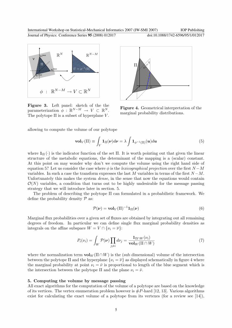