24. lecture ws 2005/06bioinformatics iii1 v17 metabolic networks - introduction different levels for...
TRANSCRIPT

24. Lecture WS 2005/06
Bioinformatics III 1
V17 Metabolic Networks - Introduction
Different levels for describing metabolic networks by computational methods:
- classical biochemical pathways (glycolysis, TCA cycle, ...
- stoichiometric modelling (flux balance analysis): theoretical capabilities of an
integrated cellular process, feasible metabolic flux distributions
- automatic decomposition of metabolic networks
(elementary nodes, extreme pathways ...)
- kinetic modelling (E-Cell ...) problem: general lack of kinetic information
on the dynamics and regulation of cellular metabolism

24. Lecture WS 2005/06
Bioinformatics III 2
EcoCyc Database
E.coli genome contains 4.7 million DNA bases.
How can we characterize the functional complement of E.coli and according to
what criteria can we compare the biochemical networks of two organisms?
EcoCyc contains the metabolic map of E.coli defined as the set of all known
pathways, reactions and enzymes of E.coli small-molecule metabolism.
Analyze
- the connectivity relationships of the metabolic network
- its partitioning into pathways
- enzyme activation and inhibition
- repetition and multiplicity of elements such as enzymes, reactions, and substrates.
Ouzonis, Karp, Genome Res. 10, 568 (2000)

24. Lecture WS 2005/06
Bioinformatics III 3
EcoCyc Analysis of E.coli Metabolism
E.coli genome contains 4391 predicted genes, of which 4288 code for proteins.
676 of these genes form 607 enzymes of E.coli small-molecule metabolism.
Of those enzymes, 311 are protein complexes, 296 are monomers.
Organization of protein complexes. Distribution of subunit counts for all EcoCyc protein complexes. The predominance of monomers, dimers, and tetramers is obvious
Ouzonis, Karp, Genome Res. 10, 568 (2000)

24. Lecture WS 2005/06
Bioinformatics III 4
ReactionsEcoCyc describes 905 metabolic reactions that are catalyzed by E. coli.
Of these reactions, 161 are not involved in small-molecule metabolism,
e.g. they participate in macromolecule metabolism such as DNA replication and
tRNA charging.
Of the remaining 744 reactions, 569 have been assigned to at least one pathway.
The next figures show an overview diagram of E. coli metabolism. Each node in
the diagram represents a single metabolite whose chemical class is encoded by
the shape of the node. Each blue line represents a single bioreaction. The white
lines connect multiple occurrences of the same metabolite in the diagram.
Ouzonis, Karp, Genome Res. 10, 568 (2000)

24. Lecture WS 2005/06
Bioinformatics III 5
Reactions
The number of reactions (744) and the number of enzymes (607) differ ...
WHY??
(1) there is no one-to-one mapping between enzymes and reactions –
some enzymes catalyze multiple reactions, and some reactions are catalyzed
by multiple enzymes.
(2) for some reactions known to be catalyzed by E.coli, the enzyme has not yet
been identified.
Ouzonis, Karp, Genome Res. 10, 568 (2000)

24. Lecture WS 2005/06
Bioinformatics III 6
Compounds
The 744 reactions of E.coli small-molecule metabolism involve a total of 791
different substrates.
On average, each reaction contains 4.0 substrates.
Number of reactions containing varying numbers of substrates (reactants plus products).
Ouzonis, Karp, Genome Res. 10, 568 (2000)

24. Lecture WS 2005/06
Bioinformatics III 7
Ouzonis, Karp, Genome Res. 10, 568 (2000)
Each distinct substrate occurs in an average of 2.1 reactions.
Compounds

24. Lecture WS 2005/06
Bioinformatics III 8
Pathways
EcoCyc describes 131 pathways:
energy metabolism
nucleotide and amino acid biosynthesis
secondary metabolism
Pathways vary in length from a
single reaction step to 16 steps
with an average of 5.4 steps.
Length distribution of EcoCyc pathways
Ouzonis, Karp, Genome Res. 10, 568 (2000)

24. Lecture WS 2005/06
Bioinformatics III 9
Reactions Catalyzed by More Than one Enzyme
Diagram showing the number of reactions
that are catalyzed by one or more enzymes.
Most reactions are catalyzed by one enzyme,
some by two, and very few by more than two
enzymes.
For 84 reactions, the corresponding enzyme is not yet encoded in EcoCyc.
What may be the reasons for isozyme redundancy?
(2) the reaction is easily „invented“; therefore, there is more than one protein family
that is independently able to perform the catalysis (convergence).
(1) the enzymes that catalyze the same reaction are homologs and have
duplicated (or were obtained by horizontal gene transfer),
acquiring some specificity but retaining the same mechanism (divergence)
Ouzonis, Karp, Genome Res. 10, 568 (2000)

24. Lecture WS 2005/06
Bioinformatics III 10
Enzymes that catalyze more than one reaction
Genome predictions usually assign a single enzymatic function.
However, E.coli is known to contain many multifunctional enzymes.
Of the 607 E.coli enzymes, 100 are multifunctional, either having the same active
site and different substrate specificities or different active sites.
Number of enzymes that catalyze one or
more reactions. Most enzymes catalyze
one reaction; some are multifunctional.
The enzymes that catalyze 7 and 9 reactions are purine nucleoside phosphorylase
and nucleoside diphosphate kinase.
Take-home message: The high proportion of multifunctional enzymes implies that
the genome projects significantly underpredict multifunctional enzymes!
Ouzonis, Karp, Genome Res. 10, 568 (2000)

24. Lecture WS 2005/06
Bioinformatics III 11
Reactions participating in more than one pathway
The 99 reactions belonging to multiple
pathways appear to be the intersection
points in the complex network of chemical
processes in the cell.
E.g. the reaction present in 6 pathways corresponds to the reaction catalyzed by
malate dehydrogenase, a central enzyme in cellular metabolism.
Ouzonis, Karp,
Genome Res. 10, 568 (2000)

24. Lecture WS 2005/06
Bioinformatics III 12
Connectivity distributions P(k) for substrates
a, Archaeoglobus fulgidus (archae);
b, E. coli (bacterium);
c, Caenorhabditis elegans (eukaryote),
shown on a log–log plot, counting
separately the incoming (In) and
outgoing links (Out) for each substrate.
kin (kout) corresponds to the number of
reactions in which a substrate
participates as a product (educt).
d, The connectivity distribution
averaged over 43 organisms.
Jeong et al. Nature 407, 651 (2000)

24. Lecture WS 2005/06
Bioinformatics III 13
Properties of metabolic networks
a, The histogram of the biochemical pathway
lengths, l, in E. coli.
b, The average path length (diameter) for
each of the 43 organisms.
c, d, Average number of incoming links (c) or
outgoing links (d) per node for each
organism.
e, The effect of substrate removal on the
metabolic network diameter of E. coli. In the
top curve (red) the most connected substrates
are removed first. In the bottom curve (green)
nodes are removed randomly. M = 60
corresponds to 8% of the total number of
substrates in found in E. coli.
The horizontal axis in b– d denotes the
number of nodes in each organism. b–d,
Archaea (magenta), bacteria (green) and
eukaryotes (blue) are shown. Jeong et al. Nature 407, 651 (2000)
The diameter of the network does notgrow with N!Diameter of smallworld network growswith log N or evenlog log N!
24. Lecture WS 2005/06
Bioinformatics III 14
Stoichiometric matrix
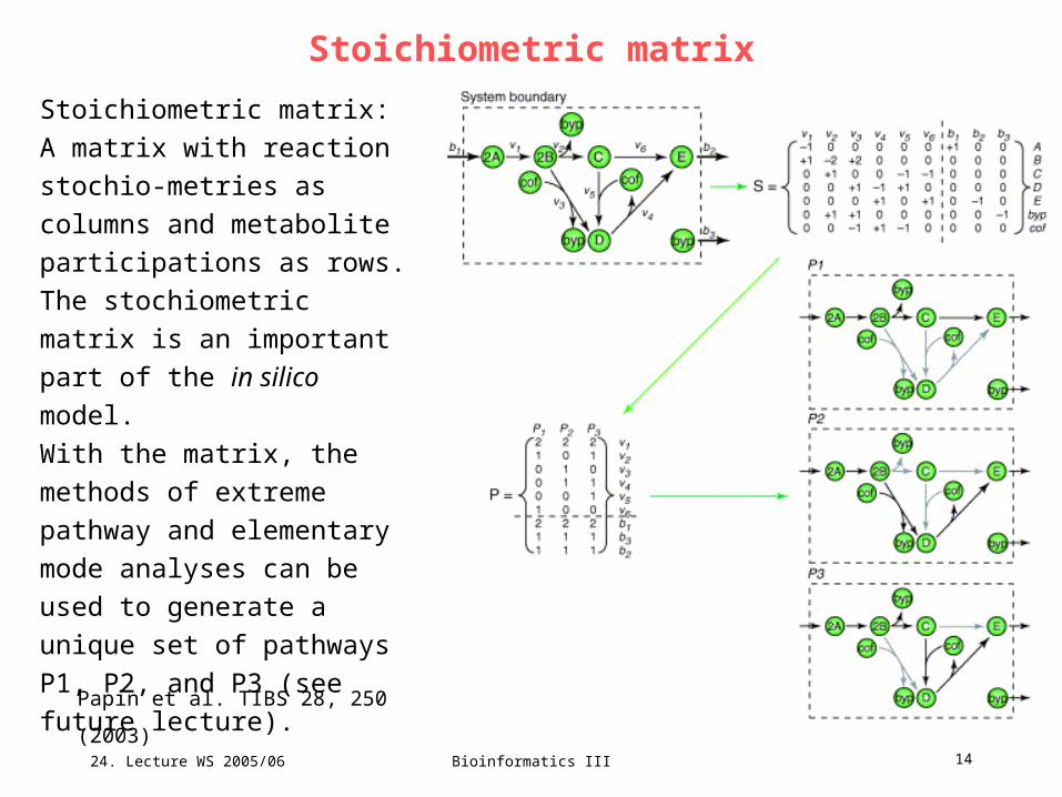
Stoichiometric matrix:
A matrix with reaction stochio-
metries as columns and
metabolite participations as
rows.
The stochiometric matrix is an
important part of the in silico
model.
With the matrix, the methods of
extreme pathway and
elementary mode analyses can
be used to generate a unique
set of pathways P1, P2, and P3
(see future lecture).
Papin et al. TIBS 28, 250 (2003)
24. Lecture WS 2005/06
Bioinformatics III 15
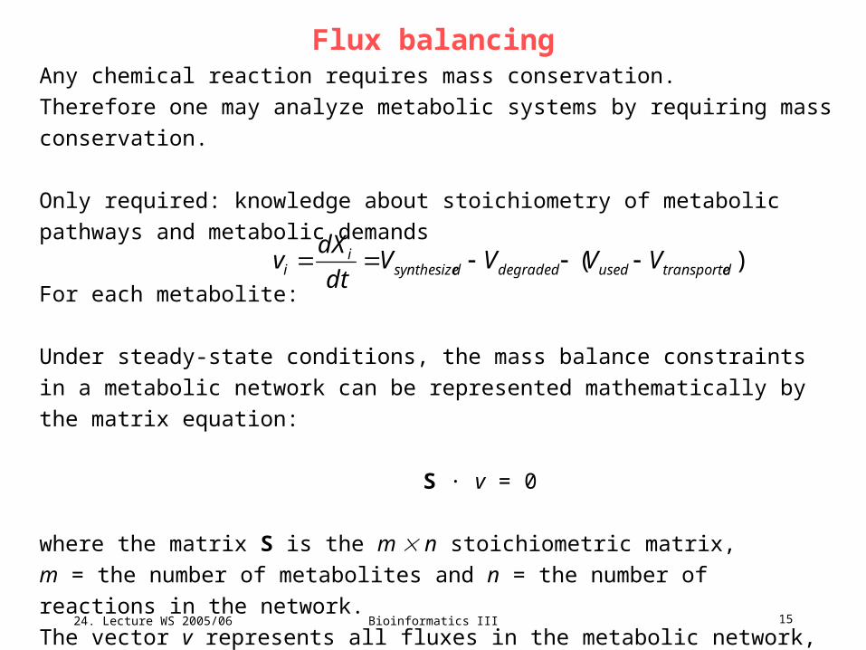
Flux balancingAny chemical reaction requires mass conservation.
Therefore one may analyze metabolic systems by requiring mass conservation.
Only required: knowledge about stoichiometry of metabolic pathways and
metabolic demands
For each metabolite:
Under steady-state conditions, the mass balance constraints in a metabolic
network can be represented mathematically by the matrix equation:
S · v = 0
where the matrix S is the m n stoichiometric matrix,
m = the number of metabolites and n = the number of reactions in the network.
The vector v represents all fluxes in the metabolic network, including the internal
fluxes, transport fluxes and the growth flux.
)( dtransporteuseddegradeddsynthesizei
i VVVVdt
dXv

24. Lecture WS 2005/06
Bioinformatics III 16
Flux balance analysis
Since the number of metabolites is generally smaller than the number of reactions
(m < n) the flux-balance equation is typically underdetermined.
Therefore there are generally multiple feasible flux distributions that satisfy the mass
balance constraints.
The set of solutions are confined to the nullspace of matrix S.
To find the „true“ biological flux in cells ( e.g. Heinzle, Huber, UdS) one needs
additional (experimental) information,
or one may impose constraints
on the magnitude of each individual metabolic flux.
The intersection of the nullspace and the region defined by those linear inequalities
defines a region in flux space = the feasible set of fluxes.
iii v
24. Lecture WS 2005/06
Bioinformatics III 17
Feasible solution set for a metabolic reaction network
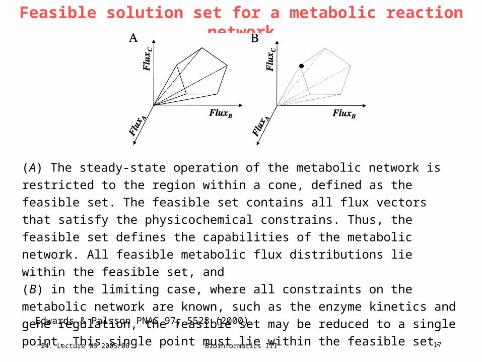
(A) The steady-state operation of the metabolic network is restricted to the region
within a cone, defined as the feasible set. The feasible set contains all flux vectors
that satisfy the physicochemical constrains. Thus, the feasible set defines the
capabilities of the metabolic network. All feasible metabolic flux distributions lie
within the feasible set, and
(B) in the limiting case, where all constraints on the metabolic network are known,
such as the enzyme kinetics and gene regulation, the feasible set may be reduced
to a single point. This single point must lie within the feasible set.
Edwards & Palsson PNAS 97, 5528 (2000)
24. Lecture WS 2005/06
Bioinformatics III 18
SummaryFBA analysis constructs the optimal network utilization simply using
stoichiometry of metabolic reactions and capacity constraints.
For E.coli the in silico results are consistent with experimental data.
FBA shows that in the E.coli metabolic network there are relatively few critical
gene products in central metabolism.
However, the the ability to adjust to different environments (growth conditions) may
be dimished by gene deletions.
FBA identifies „the best“ the cell can do, not how the cell actually behaves under a
given set of conditions. Here, survival was equated with growth.
FBA does not directly consider regulation or regulatory constraints on the
metabolic network. This can be treated separately (see future lecture).
Edwards & Palsson PNAS 97, 5528 (2000)

24. Lecture WS 2005/06
Bioinformatics III 19
V18 – extreme pathways
Price et al. Nature Rev Microbiol 2, 886 (2004)
Computational metabolomics: modelling constraints
Surviving (expressed) phenotypes must satisfy constraints imposed on the molecular
functions of a cell, e.g. conservation of mass and energy.
Fundamental approach to understand biological systems: identify and formulate
constraints.
Important constraints of cellular function:
(1) physico-chemical constraints
(2) Topological constraints
(3) Environmental constraints
(4) Regulatory constraints

24. Lecture WS 2005/06
Bioinformatics III 20
Physico-chemical constraints
Price et al. Nature Rev Microbiol 2, 886 (2004)
These are „hard“ constraints: Conservation of mass, energy and momentum.
Contents of a cell are densely packed viscosity can be 100 – 1000 times higher
than that of water
Therefore, diffusion rates of macromolecules in cells are slower than in water.
Many molecules are confined inside the semi-permeable membrane high
osmolarity. Need to deal with osmotic pressure (e.g. Na+K+ pumps)
Reaction rates are determined by local concentrations inside cells
Enzyme-turnover numbers are generally less than 104 s-1. Maximal rates are equal to
the turnover-number multiplied by the enzyme concentration.
Biochemical reactions are driven by negative free-energy change in forward
direction.

24. Lecture WS 2005/06
Bioinformatics III 21
Topological constraints
Price et al. Nature Rev Microbiol 2, 886 (2004)
The crowding of molecules inside cells leads to topological (3D)-constraints that affect
both the form and the function of biological systems.
E.g. the ratio between the number of tRNAs and the number of ribosomes in an E.coli
cell is about 10. Because there are 43 different types of tRNA, there is less than
one full set of tRNAs per ribosome it may be necessary to configure the
genome so that rare codons are located close together.
E.g. at a pH of 7.6 E.coli typically contains only about 16 H+ ions.
Remember that H+ is involved in many metabolic reactions.
Therefore, during each such reaction, the pH of the cell changes!
24. Lecture WS 2005/06
Bioinformatics III 22
Environmental constraints
Price et al. Nature Rev Microbiol 2, 886 (2004)
Environmental constraints on cells are time and condition dependent:
Nutrient availability, pH, temperature, osmolarity, availability of electron acceptors.
E.g. Heliobacter pylori lives in the human stomach at pH = 1
needs to produce NH3 at a rate that will maintain ist immediate surrounding at a pH
that is sufficiently high to allow survival.
Ammonia is made from elementary nitrogen H. pylori has adapted by using amino
acids instead of carbohydrates as its primary carbon source.

24. Lecture WS 2005/06
Bioinformatics III 23
Regulatory constraints
Price et al. Nature Rev Microbiol 2, 886 (2004)
Regulatory constraints are self-imposed by the organism and are subject to
evolutionary change they are no „hard“ constraints.
Regulatory constraints allow the cell to eliminate suboptimal phenotypic states and to
confine itself to behaviors of increased fitness.
Q: classify the following constrains asphysico-chemical, regulatory and topological restraints ...Multiple-choice selection.

24. Lecture WS 2005/06
Bioinformatics III 24
Mathematical formation of constraints
Price et al. Nature Rev Microbiol 2, 886 (2004)
There are two fundamental types of constraints: balances and bounds.
Balances are constraints that are associated
with conserved quantities as energy, mass, redox potential, momentum
or with phenomena such as solvent capacity, electroneutrality and osmotic pressure.
Bounds are constraints that limit numerical ranges of individual variables and
parameters such as concentrations, fluxes or kinetic constants.
Both bound and balance constraints limit the allowable functional states of
reconstructed cellular metabolic networks.

24. Lecture WS 2005/06
Bioinformatics III 25
Extreme Pathwaysintroduced into metabolic analysis by the lab of Bernard Palsson
(Dept. of Bioengineering, UC San Diego). The publications of this lab
are available at http://gcrg.ucsd.edu/publications/index.html
The extreme pathway
technique is based
on the stoichiometric
matrix representation
of metabolic networks.
All external fluxes are
defined as pointing outwards.
Schilling, Letscher, Palsson,
J. theor. Biol. 203, 229 (2000)

24. Lecture WS 2005/06
Bioinformatics III 26
Extreme Pathways – theorem
Theorem. A convex flux cone has a set of systemically independent generating
vectors. Furthermore, these generating vectors (extremal rays) are unique up to
a multiplication by a positive scalar. These generating vectors will be called
„extreme pathways“.
Proof. omitted.
24. Lecture WS 2005/06
Bioinformatics III 27
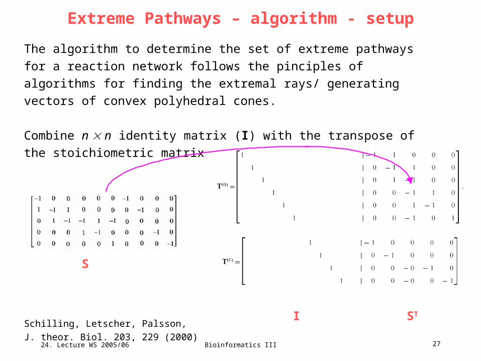
Extreme Pathways – algorithm - setup
The algorithm to determine the set of extreme pathways for a reaction network
follows the pinciples of algorithms for finding the extremal rays/ generating
vectors of convex polyhedral cones.
Combine n n identity matrix (I) with the transpose of the stoichiometric
matrix ST. I serves for bookkeeping.
Schilling, Letscher, Palsson,
J. theor. Biol. 203, 229 (2000)
S
I ST
24. Lecture WS 2005/06
Bioinformatics III 28
separate internal and external fluxes
Examine constraints on each of the exchange fluxes as given by
j bj j
If the exchange flux is constrained to be positive do nothing.
If the exchange flux is constrained to be negative multiply the
corresponding row of the initial matrix by -1.
If the exchange flux is unconstrained move the entire row to a temporary
matrix T(E). This completes the first tableau T(0).
T(0) and T(E) for the example reaction system are shown on the previous slide.
Each element of this matrices will be designated Tij.
Starting with x = 1 and T(0) = T(x-1) the next tableau is generated in the following
way:
Schilling, Letscher, Palsson,
J. theor. Biol. 203, 229 (2000)
24. Lecture WS 2005/06
Bioinformatics III 29
idea of algorithm
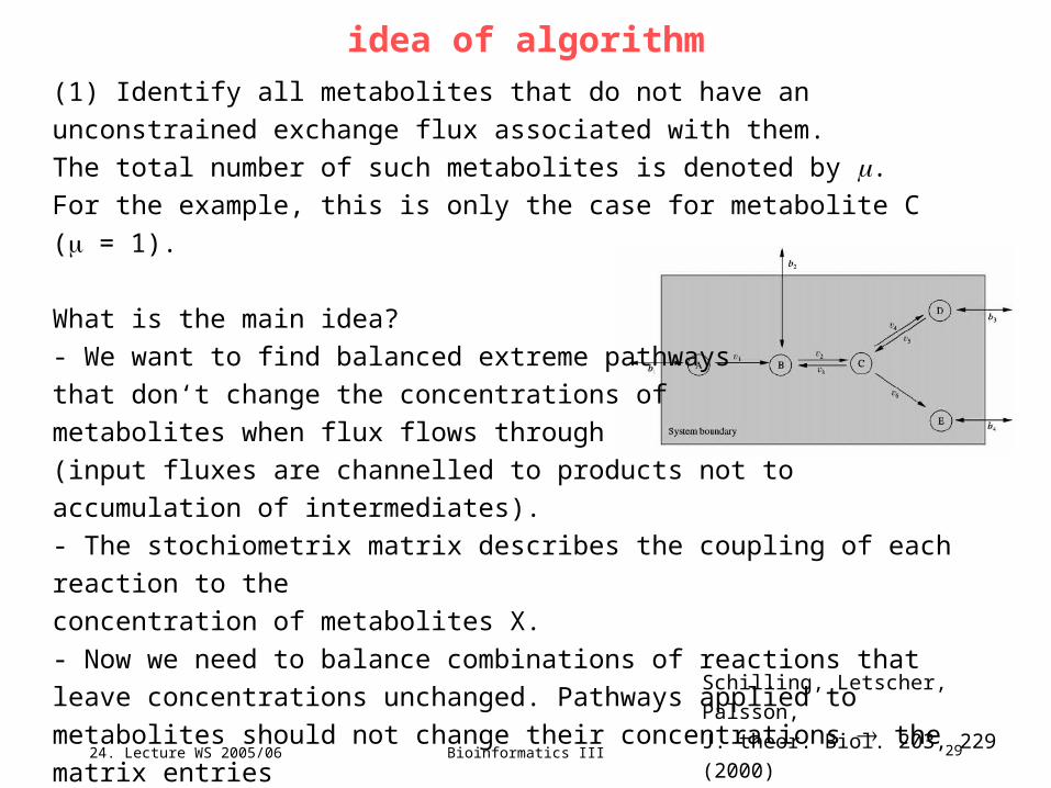
(1) Identify all metabolites that do not have an unconstrained exchange flux
associated with them.
The total number of such metabolites is denoted by .
For the example, this is only the case for metabolite C ( = 1).
What is the main idea?
- We want to find balanced extreme pathways
that don‘t change the concentrations of
metabolites when flux flows through
(input fluxes are channelled to products not to
accumulation of intermediates).
- The stochiometrix matrix describes the coupling of each reaction to the
concentration of metabolites X.
- Now we need to balance combinations of reactions that leave concentrations
unchanged. Pathways applied to metabolites should not change their
concentrations the matrix entries
need to be brought to 0.Schilling, Letscher, Palsson,
J. theor. Biol. 203, 229 (2000)

24. Lecture WS 2005/06
Bioinformatics III 30
keep pathways that do not change concentrations of internal metabolites
(2) Begin forming the new matrix T(x) by copying
all rows from T(x – 1) which contain a zero in the
column of ST that corresponds to the first
metabolite identified in step 1, denoted by index c.
(Here 3rd column of ST.)
Schilling, Letscher, Palsson, J. theor. Biol. 203, 229 (2000)
1 -1 1 0 0 0
1 0 -1 1 0 0
1 0 1 -1 0 0
1 0 0 -1 1 0
1 0 0 1 -1 0
1 0 0 -1 0 1
1 -1 1 0 0 0
T(0) =
T(1) =
+

24. Lecture WS 2005/06
Bioinformatics III 31
balance combinations of other pathways
(3) Of the remaining rows in T(x-1) add together
all possible combinations of rows which contain
values of the opposite sign in column c, such that
the addition produces a zero in this column.
Schilling, et al.
JTB 203, 229
1 -1 1 0 0 0
1 0 -1 1 0 0
1 0 1 -1 0 0
1 0 0 -1 1 0
1 0 0 1 -1 0
1 0 0 -1 0 1
T(0) =
T(1) =
1 0 0 0 0 0 -1 1 0 0 0
0 1 1 0 0 0 0 0 0 0 0
0 1 0 1 0 0 0 -1 0 1 0
0 1 0 0 0 1 0 -1 0 0 1
0 0 1 0 1 0 0 1 0 -1 0
0 0 0 1 1 0 0 0 0 0 0
0 0 0 0 1 1 0 0 0 -1 1

24. Lecture WS 2005/06
Bioinformatics III 32
remove “non-orthogonal” pathways
(4) For all of the rows added to T(x) in steps 2 and 3 check to make sure that no
row exists that is a non-negative combination of any other sets of rows in T(x) .
One method used is as follows:
let A(i) = set of column indices j for with the elements of row i = 0.
For the example above Then check to determine if there exists
A(1) = {2,3,4,5,6,9,10,11} another row (h) for which A(i) is a
A(2) = {1,4,5,6,7,8,9,10,11} subset of A(h).
A(3) = {1,3,5,6,7,9,11}
A(4) = {1,3,4,5,7,9,10} If A(i) A(h), i h
A(5) = {1,2,3,6,7,8,9,10,11} where
A(6) = {1,2,3,4,7,8,9} A(i) = { j : Ti,j = 0, 1 j (n+m) }
then row i must be eliminated from T(x)
Schilling et al.
JTB 203, 229

24. Lecture WS 2005/06
Bioinformatics III 33
repeat steps for all internal metabolites
(5) With the formation of T(x) complete steps 2 – 4 for all of the metabolites that do
not have an unconstrained exchange flux operating on the metabolite,
incrementing x by one up to . The final tableau will be T().
Note that the number of rows in T () will be equal to k, the number of extreme
pathways.
Schilling et al.
JTB 203, 229
24. Lecture WS 2005/06
Bioinformatics III 34
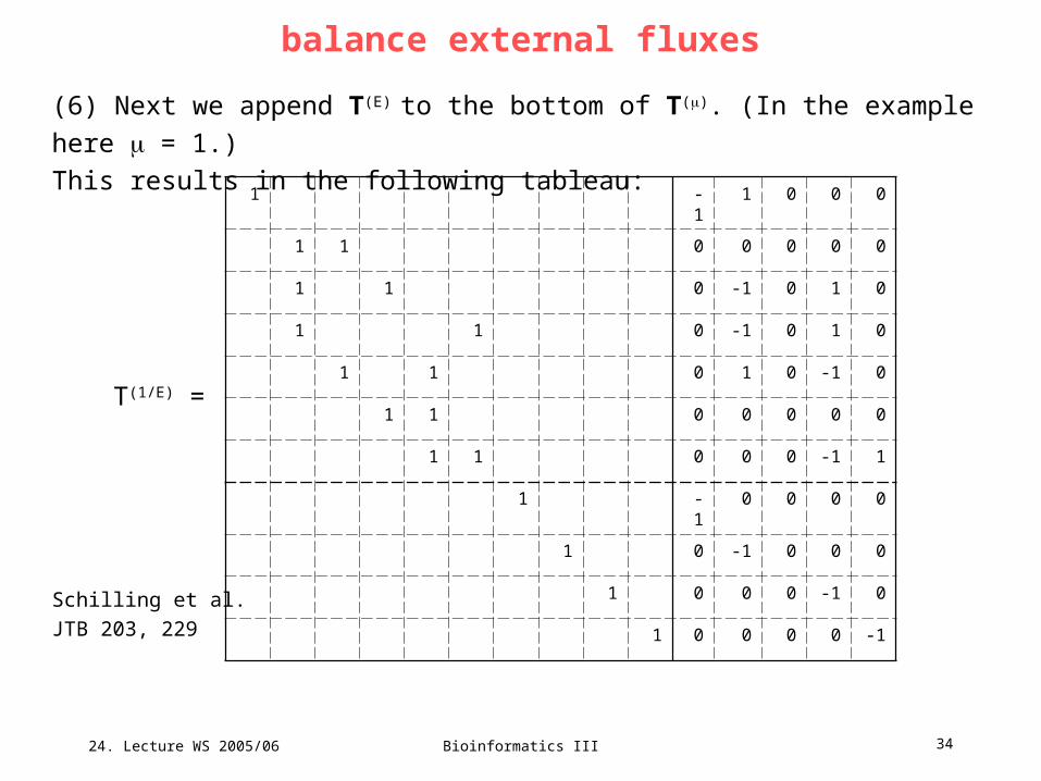
balance external fluxes
(6) Next we append T(E) to the bottom of T(). (In the example here = 1.)
This results in the following tableau:
Schilling et al.
JTB 203, 229
T(1/E) =
1 -1 1 0 0 0
1 1 0 0 0 0 0
1 1 0 -1 0 1 0
1 1 0 -1 0 1 0
1 1 0 1 0 -1 0
1 1 0 0 0 0 0
1 1 0 0 0 -1 1
1 -1 0 0 0 0
1 0 -1 0 0 0
1 0 0 0 -1 0
1 0 0 0 0 -1
24. Lecture WS 2005/06
Bioinformatics III 35
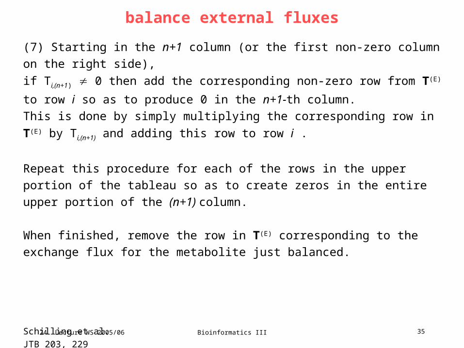
balance external fluxes
(7) Starting in the n+1 column (or the first non-zero column on the right side),
if Ti,(n+1) 0 then add the corresponding non-zero row from T(E) to row i so as to
produce 0 in the n+1-th column.
This is done by simply multiplying the corresponding row in T(E) by Ti,(n+1) and
adding this row to row i .
Repeat this procedure for each of the rows in the upper portion of the tableau so
as to create zeros in the entire upper portion of the (n+1) column.
When finished, remove the row in T(E) corresponding to the exchange flux for the
metabolite just balanced.
Schilling et al.
JTB 203, 229

24. Lecture WS 2005/06
Bioinformatics III 36
balance external fluxes
(8) Follow the same procedure as in step (7) for each of the columns on the right
side of the tableau containing non-zero entries.
(In this example we need to perform step (7) for every column except the middle
column of the right side which correponds to metabolite C.)
The final tableau T(final) will contain the transpose of the matrix P containing the
extreme pathways in place of the original identity matrix.
Schilling et al.
JTB 203, 229

24. Lecture WS 2005/06
Bioinformatics III 37
pathway matrix
T(final) =
PT =
Schilling et al.
JTB 203, 229
1 -1 1 0 0 0 0 0 0
1 1 0 0 0 0 0 0
1 1 -1 1 0 0 0 0 0 0
1 1 -1 1 0 0 0 0 0 0
1 1 1 -1 0 0 0 0 0 0
1 1 0 0 0 0 0 0
1 1 -1 1 0 0 0 0 0 0
1 0 0 0 0 0 -1 1 0 0
0 1 1 0 0 0 0 0 0 0
0 1 0 1 0 0 0 -1 1 0
0 1 0 0 0 1 0 -1 0 1
0 0 1 0 1 0 0 1 -1 0
0 0 0 1 1 0 0 0 0 0
0 0 0 0 1 1 0 0 -1 1
v1 v2 v3 v4 v5 v6 b1 b2 b3 b4
p1 p7 p3 p2 p4 p6 p5

24. Lecture WS 2005/06
Bioinformatics III 38
Extreme Pathways for model system
Schilling et al.
JTB 203, 229
1 0 0 0 0 0 -1 1 0 0
0 1 1 0 0 0 0 0 0 0
0 1 0 1 0 0 0 -1 1 0
0 1 0 0 0 1 0 -1 0 1
0 0 1 0 1 0 0 1 -1 0
0 0 0 1 1 0 0 0 0 0
0 0 0 0 1 1 0 0 -1 1
v1 v2 v3 v4 v5 v6 b1 b2 b3 b4
p1 p7 p3 p2 p4 p6 p5
2 pathways p6 and p7 are not shown (right below) because all exchange fluxes with the exterior are 0.Such pathways have no net overall effect on the functional capabilities of the network.They belong to the cycling of reactions v4/v5 and v2/v3.

24. Lecture WS 2005/06
Bioinformatics III 39
How reactions appear in pathway matrix
In the matrix P of extreme pathways, each column is an EP and each row
corresponds to a reaction in the network.
The numerical value of the i,j-th element corresponds to the relative flux level
through the i-th reaction in the j-th EP.
Papin, Price, Palsson,
Genome Res. 12, 1889 (2002)
PPP TLM

24. Lecture WS 2005/06
Bioinformatics III 40
Papin, Price, Palsson, Genome Res. 12, 1889 (2002)
A symmetric Pathway Length Matrix PLM can be calculated:
where the values along the diagonal correspond to the length of the EPs.
PPP TLM
Properties of pathway matrix
The off-diagonal terms of PLM are the number of reactions that a pair of extreme
pathways have in common.

24. Lecture WS 2005/06
Bioinformatics III 41
Papin, Price, Palsson, Genome Res. 12, 1889 (2002)
One can also compute a reaction participation matrix PPM from P:
where the diagonal correspond to the number of pathways in which the given
reaction participates.
TPM PPP
Properties of pathway matrix

24. Lecture WS 2005/06
Bioinformatics III 42
Application of elementary modesMetabolic network structure of E.coli determines
key aspects of functionality and regulation
Compute EFMs for central
metabolism of E.coli.
Catabolic part: substrate uptake
reactions, glycolysis, pentose
phosphate pathway, TCA cycle,
excretion of by-products (acetate,
formate, lactate, ethanol)
Anabolic part: conversions of
precursors into building blocks like
amino acids, to macromolecules,
and to biomass.
Stelling et al. Nature 420, 190 (2002)
Elementary modes will be covered in V19.
The concept is closely related to extreme
pathways. In this example , we will simply
ignore the small difference.

24. Lecture WS 2005/06
Bioinformatics III 43
Metabolic network topology and phenotypeThe total number of EFMs for given
conditions is used as quantitative
measure of metabolic flexibility.
a, Relative number of EFMs N enabling
deletion mutants in gene i ( i) of E. coli
to grow (abbreviated by µ) for 90 different
combinations of mutation and carbon
source. The solid line separates
experimentally determined mutant
phenotypes, namely inviability (1–40)
from viability (41–90).
Stelling et al. Nature 420, 190 (2002)
The # of EFMs for mutant strain
allows correct prediction of
growth phenotype in more than 90%
of the cases.

24. Lecture WS 2005/06
Bioinformatics III 44
Robustness analysis
The # of EFMs qualitatively indicates whether a mutant is viable or not, but does
not describe quantitatively how well a mutant grows.
Define maximal biomass yield Ymass as the optimum of:
ei is the single reaction rate (growth and substrate uptake) in EFM i selected for
utilization of substrate Sk.
Stelling et al. Nature 420, 190 (2002)
ki Si
iSXi e
eY
/,

24. Lecture WS 2005/06
Bioinformatics III 45
Compute control-effective fluxes for each reaction l by determining the efficiency of any EFM
ei by relating the system‘s output to the substrate uptake and to the sum of all absolute
fluxes.
With flux modes normalized to the total substrate uptake, efficiencies i(Sk, ) for
the targets for optimization -growth and ATP generation, are defined as:
Can regulation be predicted by EFM analysis?
Stelling et al. Nature 420, 190 (2002)
l
li
ATPi
ki
l
li
iki
e
eATPS
e
eS ,and,
Control-effective fluxes vl(Sk) are obtained by averaged weighting of the product of reaction-
specific fluxes and mode-specific efficiencies over all EFMs using the substrate under
consideration:
lki
i
liki
SAl
ki
i
liki
SXkl ATPS
eATPS
YS
eS
YSv
kk,
,1
,
,1
max/
max/
YmaxX/Si and Ymax
A/Si are optimal yields of biomass production and of ATP synthesis.
Control-effective fluxes represent the importance of each reaction for efficient and flexible
operation of the entire network.

24. Lecture WS 2005/06
Bioinformatics III 46
Prediction of gene expression patterns
As cellular control on longer timescales
is predominantly achieved by genetic
regulation, the control-effective fluxes
should correlate with messenger RNA
levels.
Compute theoretical transcript ratios
(S1,S2) for growth on two alternative
substrates S1 and S2 as ratios of
control-effective fluxes.
Compare to exp. DNA-microarray data
for E.coli growin on glucose, glycerol,
and acetate.
Excellent correlation!Stelling et al. Nature 420, 190 (2002)
Calculated ratios between gene expression levels
during exponential growth on acetate and
exponential growth on glucose (filled circles
indicate outliers) based on all elementary modes
versus experimentally determined transcript
ratios19. Lines indicate 95% confidence intervals
for experimental data (horizontal lines), linear
regression (solid line), perfect match (dashed
line) and two-fold deviation (dotted line).

24. Lecture WS 2005/06
Bioinformatics III 47
Summary (extreme pathways)
Price et al. Biophys J 84, 794 (2003)
Extreme pathway analysis provides a mathematically rigorous way to dissect
complex biochemical networks.
The matrix products PT P and PT P are useful ways to interpret pathway
lengths and reaction participation.
However, the number of computed vectors may range in the 1000sands.
Therefore, meta-methods (e.g. singular value decomposition) are required that
reduce the dimensionality to a useful number that can be inspected by humans.
Single value decomposition may be one useful method ... and there are more to
come.

24. Lecture WS 2005/06
Bioinformatics III 48
V19 Metabolic Pathway Analysis (MPA)Metabolic Pathway Analysis searches for meaningful structural and functional units
in metabolic networks.
Today‘s most powerful methods are based on convex analysis.
Two such approaches are the elementary flux modes (Schuster et al. 1999, 2000)
and extreme pathways (Schilling et al. 2000).
Both sets span the space of feasible steady-state flux distributions by
non-decomposable routes, i.e. no subset of reactions involved in an EFM
or EP can hold the network balanced using non-trivial fluxes.
MPA can be used to study e.g.
- routing + flexibility/redundancy of networks
- functionality of networks
- idenfication of futile cycles
- gives all (sub)optimal pathways with respect to product/biomass yield
- can be useful for calculability studies in MFA
Klamt et al. Bioinformatics 19, 261 (2003)

24. Lecture WS 2005/06
Bioinformatics III 49
Metabolic Pathway Analysis: Elementary Flux ModesThe technique of Elementary Flux Modes (EFM) was developed prior to extreme
pathways (EP) by Stephan Schuster, Thomas Dandekar and co-workers:
Pfeiffer et al. Bioinformatics, 15, 251 (1999)
Schuster et al. Nature Biotech. 18, 326 (2000)
The method is very similar to the „extreme pathway“ method to construct a basis
for metabolic flux states based on methods from convex algebra.
Extreme pathways are a subset of elementary modes, and for many systems, both
methods coincide.
Are the subtle differences important?
24. Lecture WS 2005/06
Bioinformatics III 50
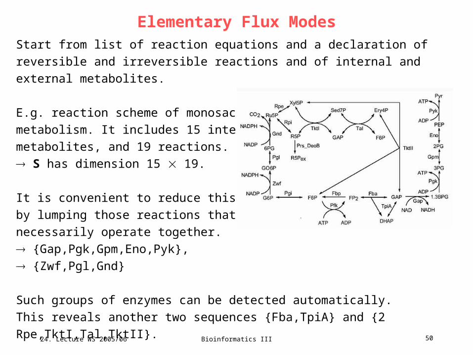
Elementary Flux ModesStart from list of reaction equations and a declaration of reversible and irreversible
reactions and of internal and external metabolites.
E.g. reaction scheme of monosaccharide Fig.1
metabolism. It includes 15 internal
metabolites, and 19 reactions.
S has dimension 15 19.
It is convenient to reduce this matrix
by lumping those reactions that
necessarily operate together.
{Gap,Pgk,Gpm,Eno,Pyk},
{Zwf,Pgl,Gnd}
Such groups of enzymes can be detected automatically.
This reveals another two sequences {Fba,TpiA} and {2 Rpe,TktI,Tal,TktII}.
Schuster et al. Nature Biotech 18, 326 (2000)
24. Lecture WS 2005/06
Bioinformatics III 51
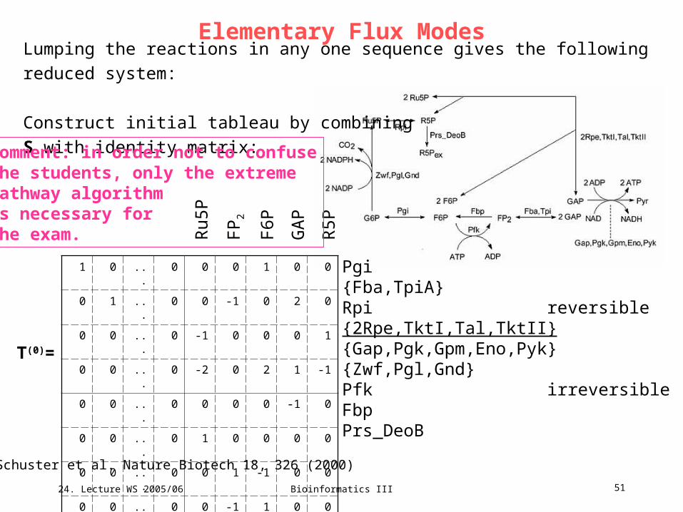
Elementary Flux ModesLumping the reactions in any one sequence gives the following reduced system:
Construct initial tableau by combining
S with identity matrix:
1 0 ... 0 0 0 1 0 0
0 1 ... 0 0 -1 0 2 0
0 0 ... 0 -1 0 0 0 1
0 0 ... 0 -2 0 2 1 -1
0 0 ... 0 0 0 0 -1 0
0 0 ... 0 1 0 0 0 0
0 0 ... 0 0 1 -1 0 0
0 0 ... 0 0 -1 1 0 0
0 0 ... 1 0 0 0 0 -1
Pgi{Fba,TpiA}Rpi reversible{2Rpe,TktI,Tal,TktII}{Gap,Pgk,Gpm,Eno,Pyk}{Zwf,Pgl,Gnd}Pfk irreversibleFbpPrs_DeoB
Schuster et al. Nature Biotech 18, 326 (2000)
Ru5
P
FP
2
F6P
GA
P
R5P
T(0)=
Comment: in order not to confusethe students, only the extremepathway algorithmis necessary forthe exam.

24. Lecture WS 2005/06
Bioinformatics III 52
Elementary Flux ModesAim again: bring all entries
of right part of matrix to 0.E.g. 2*row3 - row4 gives
„reversible“ row with 0 in column
10
New „irreversible“ rows with 0 entry
in column 10 by row3 + row6 and
by row4 + row7.
In general, linear combinations
of 2 rows corresponding
to the same type of directio-
nality go into the part of
the respective type in the
tableau. Combinations by
different types go into the
„irreversible“ tableau
because at least 1 reaction is
irreversible. Irreversible reactions
can only combined using positive
coefficients.Schuster et al. Nature Biotech 18, 326 (2000)
1 0 0 1 0 0
1 0 -1 0 2 0
1 -1 0 0 0 1
1 -2 0 2 1 -1
1 0 0 0 -1 0
1 1 0 0 0 0
1 0 1 -1 0 0
1 0 -1 1 0 0
1 0 0 0 0 -1
1 0 0 1 0 0
1 0 -1 0 2 0
2 -1 0 0 -2 -1 3
1 0 0 0 -1 0
1 0 1 -1 0 0
1 0 -1 1 0 0
1 0 0 0 0 -1
1 1 0 0 0 0 1
1 2 0 0 2 1 -1
T(1)=
T(0)=

24. Lecture WS 2005/06
Bioinformatics III 53
Elementary Flux ModesAim: zero column 11.Include all possible (direction-wise
allowed) linear combinations of
rows.
continue with columns 12-
14. Schuster et al. Nature Biotech 18, 326 (2000)
1 0 0 1 0 0
1 0 -1 0 2 0
2 -1 0 0 -2 -1 3
1 0 0 0 -1 0
1 0 1 -1 0 0
1 0 -1 1 0 0
1 0 0 0 0 -1
1 1 0 0 0 0 1
1 2 0 0 2 1 -1
1 0 0 1 0 0
2 -1 0 0 -2 -1 3
1 0 0 0 -1 0
1 0 0 0 0 -1
1 1 0 0 0 0 1
1 2 0 0 2 1 -1
1 1 0 0 -1 2 0
-1 1 0 0 1 -2 0
1 1 0 0 0 0 0
T(2)=
T(1)=

24. Lecture WS 2005/06
Bioinformatics III 54
Elementary Flux ModesIn the course of the algorithm, one must avoid
- calculation of nonelementary modes (rows that contain fewer zeros than the row
already present)
- duplicate modes (a pair of rows is only combined if it fulfills the condition
S(mi(j)) S(mk
(j)) S(ml(j+1)) where S(ml
(j+1)) is the set of positions of 0 in this row.
- flux modes violating the sign restriction for the irreversible reactions.
Final tableau
T(5) =
This shows that the number of rows may decrease or increase in the course of the
algorithm. All constructed elementary modes are irreversible.
Schuster et al. Nature Biotech 18, 326 (2000)
1 1 0 0 2 0 1 0 0 0 ... ... 0
-2 0 1 1 1 3 0 0 0 ... ...
0 2 1 1 5 3 2 0 0
0 0 1 0 0 1 0 0 1
5 1 4 -2 0 0 1 0 6
-5 -1 2 2 0 6 0 1 0 ... ...
0 0 0 0 0 0 1 1 0 0 ... ... 0

24. Lecture WS 2005/06
Bioinformatics III 55
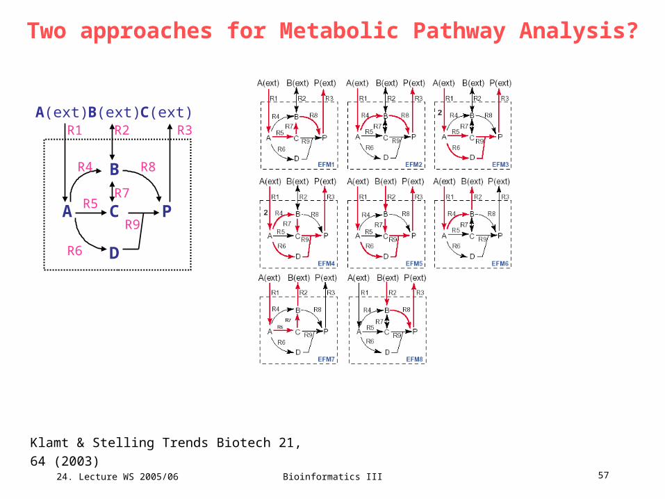
Two approaches for Metabolic Pathway Analysis?A pathway P(v) is an elementary flux mode if it fulfills conditions C1 – C3.
(C1) Pseudo steady-state. S e = 0. This ensures that none of the
metabolites is consumed or produced in the overall stoichiometry.
(C2) Feasibility: rate ei 0 if reaction is irreversible. This demands that only
thermodynamically realizable fluxes are contained in e.
(C3) Non-decomposability: there is no vector v (unequal to the zero vector
and to e) fulfilling C1 and C2 and that P(v) is a proper subset of P(e). This is
the core characteristics for EFMs and EPs and supplies the decomposition
of the network into smallest units (able to hold the network in steady state).
C3 is often called „genetic independence“ because it implies that the
enzymes in one EFM or EP are not a subset of the enzymes from another
EFM or EP.
Klamt & Stelling Trends Biotech 21, 64 (2003)

24. Lecture WS 2005/06
Bioinformatics III 56
Two approaches for Metabolic Pathway Analysis?The pathway P(e) is an extreme pathway if it fulfills conditions C1 – C3 AND
conditions C4 – C5.
(C4) Network reconfiguration: Each reaction must be classified either as
exchange flux or as internal reaction. All reversible internal reactions must
be split up into two separate, irreversible reactions (forward and backward
reaction).
(C5) Systemic independence: the set of EPs in a network is the minimal set
of EFMs that can describe all feasible steady-state flux distributions.
Klamt & Stelling Trends Biotech 21, 64 (2003)
24. Lecture WS 2005/06
Bioinformatics III 57
Two approaches for Metabolic Pathway Analysis?
Klamt & Stelling Trends Biotech 21, 64 (2003)
A C P
B
D
A(ext) B(ext) C(ext)R1 R2 R3
R5
R4 R8
R9
R6
R7

24. Lecture WS 2005/06
Bioinformatics III 58
Reconfigured Network
Klamt & Stelling Trends Biotech 21, 64 (2003)
A C P
B
D
A(ext) B(ext) C(ext)R1 R2 R3
R5
R4 R8
R9
R6
R7bR7f
3 EFMs are not systemically independent:EFM1 = EP4 + EP5EFM2 = EP3 + EP5EFM4 = EP2 + EP3

24. Lecture WS 2005/06
Bioinformatics III 59
Property 1 of EFMs
Klamt & Stelling Trends Biotech 21, 64 (2003)
The only difference in the set of EFMs emerging upon reconfiguration consists in
the two-cycles that result from splitting up reversible reactions. However, two-
cycles are not considered as meaningful pathways.
Valid for any network: Property 1
Reconfiguring a network by splitting up reversible reactions leads to the same set of
meaningful EFMs.

24. Lecture WS 2005/06
Bioinformatics III 60
Software: FluxAnalyzerWhat is the consequence of when all exchange fluxes (and hence all
reactions in the network) are irreversible?
Klamt & Stelling Trends Biotech 21, 64 (2003)
Then EFMs and EPs always co-incide!

24. Lecture WS 2005/06
Bioinformatics III 61
Property 2 of EFMs
Klamt & Stelling Trends Biotech 21, 64 (2003)
Property 2
If all exchange reactions in a network are irreversible then the sets of
meaningful EFMs (both in the original and in the reconfigured network) and
EPs coincide.

24. Lecture WS 2005/06
Bioinformatics III 62
Reconfigured Network
Klamt & Stelling Trends Biotech 21, 64 (2003)
A C P
B
D
A(ext) B(ext) C(ext)R1 R2 R3
R5
R4 R8
R9
R6
R7bR7f
3 EFMs are not systemically independent:EFM1 = EP4 + EP5EFM2 = EP3 + EP5EFM4 = EP2 + EP3
24. Lecture WS 2005/06
Bioinformatics III 63
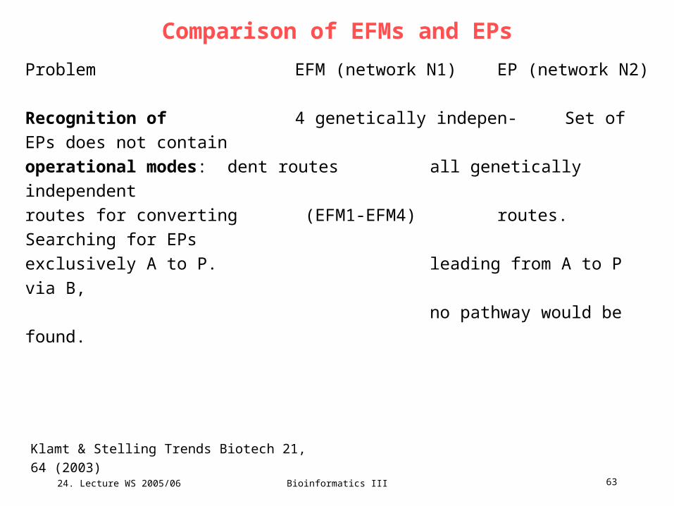
Comparison of EFMs and EPs
Klamt & Stelling Trends Biotech 21, 64 (2003)
Problem EFM (network N1) EP (network N2)
Recognition of 4 genetically indepen- Set of EPs does not contain
operational modes: dent routes all genetically independent
routes for converting (EFM1-EFM4) routes. Searching for EPs
exclusively A to P. leading from A to P via B,
no pathway would be found.

24. Lecture WS 2005/06
Bioinformatics III 64
Comparison of EFMs and EPs
Klamt & Stelling Trends Biotech 21, 64 (2003)
Problem EFM (network N1) EP (network N2)
Finding all the EFM1 and EFM2 are One would only find the
optimal routes: optimal because they suboptimal EP1, not the
optimal pathways for yield one mole P per optimal routes EFM1 and
synthesizing P during mole substrate A EFM2.
growth on A alone. (i.e. R3/R1 = 1),
whereas EFM3 and
EFM4 are only sub-
optimal (R3/R1 = 0.5).

24. Lecture WS 2005/06
Bioinformatics III 65
Comparison of EFMs and EPs
Klamt & Stelling Trends Biotech 21, 64 (2003)
EFM (network N1)
4 pathways convert A
to P (EFM1-EFM4),
whereas for B only one
route (EFM8) exists.
When one of the
internal reactions (R4-
R9) fails, for production
of P from A 2 pathways
will always „survive“. By
contrast, removing
reaction R8 already
stops the production of
P from B alone.
EP (network N2)
Only 1 EP exists for
producing P by substrate A
alone, and 1 EP for
synthesizing P by (only)
substrate B. One might
suggest that both
substrates possess the
same redundancy of
pathways, but as shown by
EFM analysis, growth on
substrate A is much more
flexible than on B.
Problem
Analysis of network
flexibility (structural
robustness,
redundancy):
relative robustness of
exclusive growth on
A or B.

24. Lecture WS 2005/06
Bioinformatics III 66
Comparison of EFMs and EPs
Klamt & Stelling Trends Biotech 21, 64 (2003)
EFM (network N1)
R8 is essential for
producing P by substrate
B, whereas for A there is
no structurally „favored“
reaction (R4-R9 all occur
twice in EFM1-EFM4).
However, considering the
optimal modes EFM1,
EFM2, one recognizes the
importance of R8 also for
growth on A.
EP (network N2)
Consider again biosynthesis
of P from substrate A (EP1
only). Because R8 is not
involved in EP1 one might
think that this reaction is not
important for synthesizing P
from A. However, without this
reaction, it is impossible to
obtain optimal yields (1 P per
A; EFM1 and EFM2).
Problem
Relative importance
of single reactions:
relative importance of
reaction R8.

24. Lecture WS 2005/06
Bioinformatics III 67
Comparison of EFMs and EPs
Klamt & Stelling Trends Biotech 21, 64 (2003)
EFM (network N1)
R6 and R9 are an enzyme
subset. By contrast, R6
and R9 never occur
together with R8 in an
EFM. Thus (R6,R8) and
(R8,R9) are excluding
reaction pairs.(In an arbitrary composable
steady-state flux distribution they
might occur together.)
EP (network N2)
The EPs pretend R4 and R8
to be an excluding reaction
pair – but they are not
(EFM2). The enzyme
subsets would be correctly
identified. However, one can construct simple
examples where the EPs would also
pretend wrong enzyme subsets (not
shown).
Problem
Enzyme subsets
and excluding
reaction pairs:
suggest regulatory
structures or rules.

24. Lecture WS 2005/06
Bioinformatics III 68
Comparison of EFMs and EPs
Klamt & Stelling Trends Biotech 21, 64 (2003)
EFM (network N1)
The shortest pathway
from A to P needs 2
internal reactions (EFM2),
the longest 4 (EFM4).
EP (network N2)
Both the shortest (EFM2)
and the longest (EFM4)
pathway from A to P are not
contained in the set of EPs.
Problem
Pathway length:
shortest/longest
pathway for
production of P from
A.

24. Lecture WS 2005/06
Bioinformatics III 69
Comparison of EFMs and EPs
Klamt & Stelling Trends Biotech 21, 64 (2003)
EFM (network N1)
All EFMs not involving the
specific reactions build up
the complete set of EFMs
in the new (smaller) sub-
network. If R7 is deleted,
EFMs 2,3,6,8 „survive“.
Hence the mutant is
viable.
EP (network N2)
Analyzing a subnetwork
implies that the EPs must be
newly computed. E.g. when
deleting R2, EFM2 would
become an EP. For this
reason, mutation studies
cannot be performed easily.
Problem
Removing a
reaction and
mutation studies:
effect of deleting R7.

24. Lecture WS 2005/06
Bioinformatics III 70
Comparison of EFMs and EPs
Klamt & Stelling Trends Biotech 21, 64 (2003)
EFM (network N1)
For the case of R7, all
EFMs but EFM1 and
EFM7 „survive“ because
the latter ones utilize R7
with negative rate.
EP (network N2)
In general, the set of EPs
must be recalculated:
compare the EPs in network
N2 (R2 reversible) and N4
(R2 irreversible).
Problem
Constraining
reaction
reversibility:
effect of R7 limited to
B C.
Q: Discuss the relevance of the elementary modes 1 to Xfor the following properties ...

24. Lecture WS 2005/06
Bioinformatics III 71
Minimal cut sets in biochemical reaction networksConcept of minimal cut sets (MCSs): smallest „failure modes“ in the network
that render the correct functioning of a cellular reaction impossible.
Klamt & Gilles, Bioinformatics 20, 226 (2004)
Right: fictitious reaction network NetEx.
The only reversible reaction is R4.
We are particularly interested in the flux
obR exporting synthesized metabolite X.
Characterize solution space by
computing elementary modes.

24. Lecture WS 2005/06
Bioinformatics III 72
Elementary modes of NetEx
Klamt & Gilles, Bioinformatics 20, 226 (2004)
One finds 4 elementary modes for NetEx.
3 of them (shaded) allow the production of metabolite X.

24. Lecture WS 2005/06
Bioinformatics III 73
Cut set
Klamt & Gilles, Bioinformatics 20, 226 (2004)
Now we want to prevent the production of metabolite X.
demand that there is no balanced flux distribution possible which involves obR.
Definition. We call a set of reactions a cut set (with respect to a defined
objective reaction) if after the removal of these reactions from the network no
feasible balanced flux distribution involves the objective reaction.
A trivial cut set if the reaction itself: C0 = {obR}. Why should we be interested in
other solutions as well?
- From an engineering point of view, it might be desirable to cut reactions at the
beginning of a pathway.
- The production of biomass is usually not coupled to a single gene or enzyme, and
can therefore not be directly inactivated.

24. Lecture WS 2005/06
Bioinformatics III 74
Cut set
Klamt & Gilles, Bioinformatics 20, 226 (2004)
Another extreme case is the removal of all reactions except obR .. not efficient!
E.g. C1 = {R5,R8} is a cut set already
sufficient for preventing the production of X.
Removing R5 or R8 alone is not sufficient.
C1 is a minimal cut set
Definition. A cut set C (related to a
defined objective reaction) is a
minimal cut set (MCS) if no proper
subset of C is a cut set.
Q: discuss the following minimal cut sets MCS1, MCS2.

24. Lecture WS 2005/06
Bioinformatics III 75
Remarks
Klamt & Gilles, Bioinformatics 20, 226 (2004)
(1) An MCS always guarantees dysfunction as long as the assumed network
structure is currect. However, additional regulatory circuits or capacity restrictions
may allow that even a proper subset of a MCS is a cut set.
The MCS analysis should always be seen from a purely structural point of view.
(2) After removing a complete MCS from the network, other pathways producing
other metabolites may still be active.
(3) MCS4 = {R5,R8} clearly stops production of X.
What about MCS6 = {R3,R4,R6}?
Cannot X be still be produced via R1, R2, and R5?
However, this would lead to accumulation of B and is therefore physiologically
impossible.

24. Lecture WS 2005/06
Bioinformatics III 76
Algorithm for computing MCSs
Klamt & Gilles, Bioinformatics 20, 226 (2004)
The MCSs for a given network and objective reaction are members of the power
set of the set of reaction indices and are uniquely determined.
A systematic computation must ensure that the calculated MCSs are:
(1) cut sets („destroying“ all possible balanced flux distributions involving the
objective reaction), and
(2) that the MCSs are really minimal, and
(3) that all MCSs are found.
Algorithm given in lecture is omitted.
24. Lecture WS 2005/06
Bioinformatics III 77
Applications of MCSs
Klamt & Gilles, Bioinformatics 20, 226 (2004)
Target identification and repressing cellular functions
A screening of all MCSs allows for the identification of the best suitable
manipulation. For practical reasons, the following conditions should be fulfilled:
- usually, a small number of interventions is desirable (small size of MCS)
- other pathways in the network should only be weakly affected
- some of the cellular functions might be difficult to run off genetically or by
inhibition, e.g. if many isozymes exist for a reaction.

24. Lecture WS 2005/06
Bioinformatics III 78
Applications of MCSs
Klamt & Gilles, Bioinformatics 20, 226 (2004)
Structural fragility and robustness
If we assume that each reaction in a metabolic network has the same probability to
fail, small MCSs are most probable to be responsible for a failing objective function.
Define a fragility coefficient Fi as the
reciprocal of the average size of all
MCSs in which reaction i participates.
Besides the essential reaction R1, reactionR5 is most crucial for the objective reaction.
Q: give the definition of the fragility coefficientand discuss its meaning.

24. Lecture WS 2005/06
Bioinformatics III 79
Conclusion
Klamt & Gilles, Bioinformatics 20, 226 (2004)
An MCS is a irreducible combination of network elements whose simultaneous
inactivation leads to a guaranteed dysfunction of certain cellular reactions or
processes.
MCSs are inherent and uniquely determined structural features of metabolic
networks similar to EMs.
The computation of MCSs and EMs becomes challenging in large networks.
Analyzing the MCSs gives deeper insights in the structural fragility of a given
metabolic network and is useful for identifying target sets for an intended
repression of network functions.

24. Lecture WS 2005/06
Bioinformatics III 80
V20 The Double Description method:Theoretical framework behind EFM and EP
in „Combinatorics and Computer Science Vol. 1120“ edited by Deza, Euler, Manoussakis, Springer, 1996:91

24. Lecture WS 2005/06
Bioinformatics III 81
Definition of Elementary ModesCompared to gene regulatory processes, metabolism involves fast reactions and
high turnover of substances.
it is often assumed that metabolite concentrations and reaction rates are
equilibrated (constant) on the timescale of study.
The metabolic system is then considered to be in quasi steady state implying
S v = 0 , S: stoichiometric matrix, v: feasible flux distributions.
Thermodynamics imposes the rate of each irreversible reaction to be nonnegative.
Consequently the set of feasible flux vectors is restricted to
P = {v q : S v = 0 and vi ≥ 0, i Irrev} (1)
P is a set of q-vectors that obey a finite set of homogeneous linear equalities and
inequalities, namely
- the |Irrev| inequalities defined by vi ≥ 0, i Irrev and
- the m equalities defined by S v = 0.

24. Lecture WS 2005/06
Bioinformatics III 82
Elementary Flux Modes
Metabolic pathway analysis serves to describe the infinite set P of feasible states by
providing a finite set of vectors that allow the generation of any vectors of P and are
of fundamental importance for the overall capabilities of the metabolic system.
One of these sets is the so-called set of elementary (flux) modes (EMs).
For a given flux vector v, we note R(v) = {i : vi ≠ 0} the set of indices of the reactions
participating in v.
R(v) can be seen as the underlying pathway of v.
24. Lecture WS 2005/06
Bioinformatics III 83
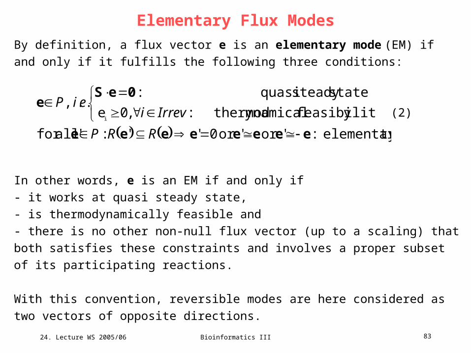
Elementary Flux Modes
By definition, a flux vector e is an elementary mode (EM) if and only if it fulfills the
following three conditions:
(2)
In other words, e is an EM if and only if
- it works at quasi steady state,
- is thermodynamically feasible and
- there is no other non-null flux vector (up to a scaling) that both satisfies these
constraints and involves a proper subset of its participating reactions.
With this convention, reversible modes are here considered as two vectors of
opposite directions.
tyelementari :'or 'or 0'':' allfor
yfeasibilit ynamical thermod:,0e
statesteady quasi :.. ,
i
eeeeeeee
0eSe
RRP
IrrevieiP

24. Lecture WS 2005/06
Bioinformatics III 84
In the particular case of a metabolic system with only irreversible reactions,
the set of admissible reactions reads:
P = {v q : S v = 0 and vi 0, i Irrev } (3)
P is in this case a pointed polyhedral cone.
The set of feasible metabolic fluxes described before is therefore – by definition –
a convex polyhedral cone.
A unified framework - Elementary modes as extreme rays in networks of irreversible reactions
A pointed polyhedral cone. Dashed lines represent virtual cuts of unbounded areas

24. Lecture WS 2005/06
Bioinformatics III 85
Pointed polyhedral cone – more precise
Definition P is a pointed polyhedral cone of d if and only if P is defined by a
full rank h × d matrix A (rank(A) = d) such that,
Insert: the rank of a matrix is the dimension of the range of the matrix,
corresponding to the number of linearly independent rows or columns of the matrix.
The h rows of the matrix A represent h linear inequalities, whereas the full rank
mention imposes the "pointed" effect in 0. Note that a pointed polyhedral cone is,
in general, not restricted to be located completely in the positive orphant as in (3).
For example, the cone considered in extreme-pathway analysis may have
negative parts (namely for exchange reactions), however, by using a particular
configuration it is ensured that the spanned cone is pointed.
P = P(A) = {x d : A x 0}

24. Lecture WS 2005/06
Bioinformatics III 86
Extreme rays
A vector r is said to be a ray of P(A) if r ≠ 0 and for all α > 0, α · r P(A).
We identify two rays r and r' if there is some α > 0 such that r = α · r' and we
denote r ≃ r', analogous as introduced above for flux vectors.
For any vector x in P(A), the zero set or active set Z(x) is the set of inequality
indices satisfied by x with equality.
Noting Ai• the ith row of A, Z(x) = {i : Ai•x = 0}.
Zero sets can be used to characterize extreme rays.

24. Lecture WS 2005/06
Bioinformatics III 87
Extreme rays - definition
Definition 1
Let r be a ray of the pointed polyhedral cone P(A).
The following statements are equivalent:
(a) r is an extreme ray of P(A)
(b) if r' is a ray of P(A) with Z(r) Z(r') then r' ≃ r
Since A is full rank, 0 is the unique vector that solves all constraints with equality.
The extreme rays are those rays of P(A) that solve a maximum but not all
constraints with equalities. This is expressed in (b) by requiring that no other ray in P(A) solves the same constraints plus additional ones with equalities.
Note that in (b) Z(r) = Z(r') consequently holds.

24. Lecture WS 2005/06
Bioinformatics III 88
Extreme rays - propertiesAn important property of the extreme rays is that they form a finite set of
generating vectors of the pointed cone:
any vector of P(A) can be expressed as a non-negative linear combination of
extreme rays,
The converse is also true:
all non-negative combinations of extreme rays lie in P(A).
The set of extreme rays is the unique minimal set of generating vectors of
a pointed cone P(A) (up to positive scalings).

24. Lecture WS 2005/06
Bioinformatics III 89
Elementary modes
Lemma 1: EMs in networks of irreversible reactions
In a metabolic system where all reactions are irreversible, the EMs are exactly the
extreme rays of P = {v q : S v = 0 and v ≥ 0}.
Proof: omitted. □

24. Lecture WS 2005/06
Bioinformatics III 90
The general caseIn the general case, some reactions of the metabolic system can be reversible.
Consequently, A does not contain the identity matrix and P (as given in (1))
is not ensured to be a pointed polyhedral cone anymore.
Because they contain a linear subspace, non-pointed polyhedral cones cannot be
represented properly by a unique set of generating vectors composed of extreme
rays.
One way to obtain a pointed polyhedral cone from (1) is to split up each reversible
reaction into two opposite irreversible ones.
(This is routinely done for the construction of extreme pathways.
Therefore, EPs directly correspond to a flux cone).
This virtual split essentially does not change the outcome:
the EMs in the reconfigured network are practically equivalent
to the EMs from the original network.
24. Lecture WS 2005/06
Bioinformatics III 91
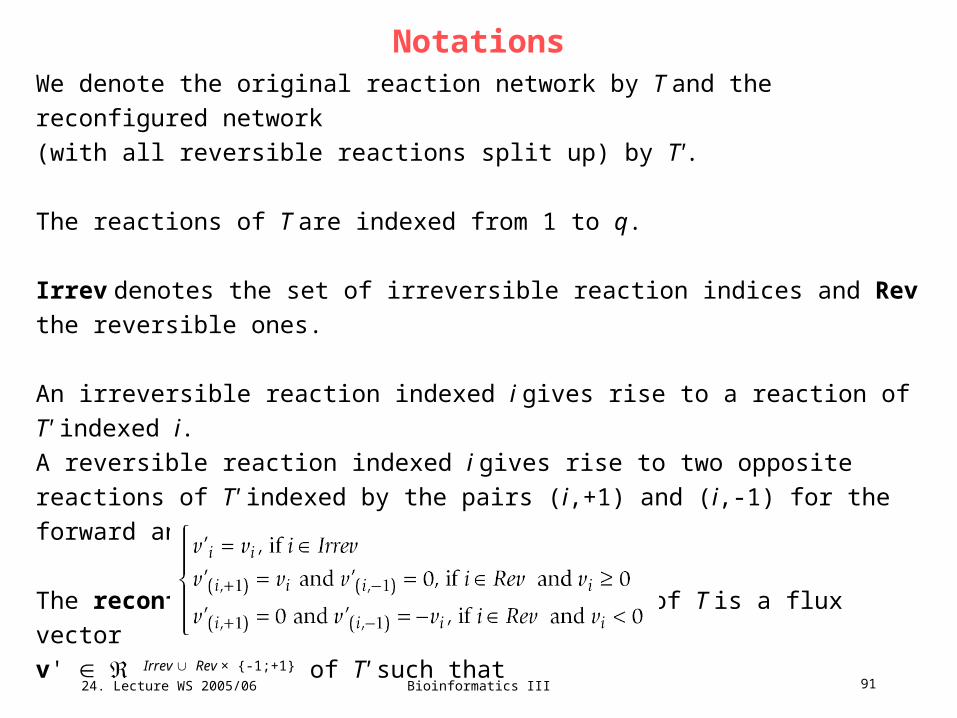
NotationsWe denote the original reaction network by T and the reconfigured network
(with all reversible reactions split up) by T'.
The reactions of T are indexed from 1 to q.
Irrev denotes the set of irreversible reaction indices and Rev the reversible ones.
An irreversible reaction indexed i gives rise to a reaction of T' indexed i.
A reversible reaction indexed i gives rise to two opposite reactions of T' indexed by
the pairs (i,+1) and (i,-1) for the forward and the backward respectively.
The reconfiguration of a flux vector v q of T is a flux vector
v' Irrev Rev × {-1;+1} of T' such that

24. Lecture WS 2005/06
Bioinformatics III 92
Notations
Let S' be the stoichiometry matrix of T'. S' can be written as S' = [S –SRev] where
SRev consists of all columns of S corresponding to reversible reactions.
Note that if v is a flux vector of T and v' is its reconfiguration then S v = S' v'.
If possible, i.e. if v' Irrev Rev × {-1;+1} is such that for any reversible reaction index
i Rev at least one of the two coefficients v'(i,+1) or v'(i,-1) equals zero,
then we define the reverse operation, called back-configuration that maps v' back to
a flux vector v such that:

24. Lecture WS 2005/06
Bioinformatics III 93
Theorem 1: EMs in original and in reconfigured networks
Theorem 1
Let T be a metabolic system and T' its reconfiguration by splitting up
reversible reactions.
Then the set of EMs of T' is the union of
a) the set of reconfigured EMs of T
b) the set of two-cycles made of a forward and a backward reaction
of T' derived from the same reversible reaction of T.
Proof. omitted.

24. Lecture WS 2005/06
Bioinformatics III 94
Double Description Method (1953)
All known algorithms for computing EMs are variants of the
Double Description Method.
- derive simple & efficient algorithm for extreme ray enumeration, the so-called
Double Description Method.
- show that it serves as a framework to the popular EM computation methods.

24. Lecture WS 2005/06
Bioinformatics III 95
The Double Description MethodA pair (A,R) of real matrices A and R is said to be a double description pair or
simply a DD pair if the relationship
A x 0 if and only if x = R for some 0
holds. Clearly, for a pair (A,R) to be a DD pair, the column size of A has to
equal the row size of R, say d.
For such a pair,
the set P(A) represented by A as
is simultaneously represented by R as
A subset P of d is called polyhedral cone if P = P(A) for some matrix A,
and A is called a representation matrix of the polyhedral cone P(A).
Then, we say R is a generating matrix for P. Clearly, each column vector of a
generating matrix R lies in the cone P and every vector in P is a nonnegative
combination of some columns of R.
0: AxxA dP
0 somefor : λRλxx d

24. Lecture WS 2005/06
Bioinformatics III 96
The Double Description MethodTheorem 1 (Minkowski‘s Theorem for Polyhedral Cones)
For any m n real matrix A, there exists some d m real matrix R such that
(A,R) is a DD pair, or in other words, the cone P(A) is generated by R.
The theorem states that every polyhedral cone admits a generating matrix.
The nontriviality comes from the fact that the row size of R is finite.
If we allow an infinite size, there is a trivial generating matrix consisting of all
vectors in the cone.
Also the converse is true:
Theorem 2 (Weyl‘s Theorem for Polyhedral Cones)
For any d n real matrix R, there exists some m d real matrix A such that (A,R)
is a DD pair, or in other words, the set generated by R is the cone P(A).

24. Lecture WS 2005/06
Bioinformatics III 97
The Double Description MethodTask: how does one construct a matrix R from a given matrix A, and the converse?
These two problems are computationally equivalent.
Farkas‘ Lemma shows that (A,R) is a DD pair if and only if (RT,AT) is a DD pair.
A more appropriate formulation of the problem is to require the minimality of R:
find a matrix R such that no proper submatrix is generating P(A).
A minimal set of generators is unique up to positive scaling when we assume the
regularity condition that the cone is pointed, i.e. the origin is an extreme point of
P(A).
Geometrically, the columns of a minimal generating matrix are in 1-to-1
correspondence with the extreme rays of P.
Thus the problem is also known as the extreme ray enumeration problem.
No efficient (polynomial) algorithm is known for the general problem.
24. Lecture WS 2005/06
Bioinformatics III 98
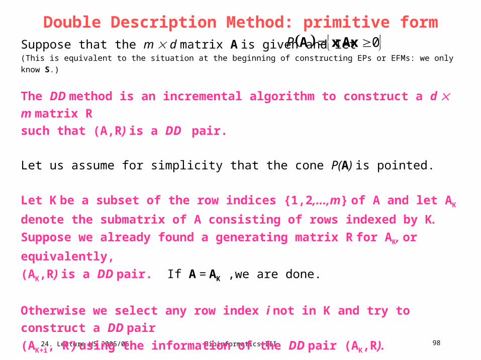
Double Description Method: primitive formSuppose that the m d matrix A is given and let(This is equivalent to the situation at the beginning of constructing EPs or EFMs: we only know S.)
The DD method is an incremental algorithm to construct a d m matrix R
such that (A,R) is a DD pair.
Let us assume for simplicity that the cone P(A) is pointed.
Let K be a subset of the row indices {1,2,...,m} of A and let AK denote the
submatrix of A consisting of rows indexed by K.
Suppose we already found a generating matrix R for AK, or equivalently,
(AK,R) is a DD pair. If A = AK ,we are done.
Otherwise we select any row index i not in K and try to construct a DD pair
(AK+i, R‘) using the information of the DD pair (AK,R).
Once this basic procedure is described, we have an algorithm to construct a
generating matrix R for P(A).
0 AxxA :P

24. Lecture WS 2005/06
Bioinformatics III 99
Geometric version of iteration stepThe procedure can be easily understood geometrically by looking at the
cut-section C of the cone P(AK) with some appropriate hyperplane h in d
which intersects with every extreme ray of P(AK) at a single point.
Let us assume that the cone is pointed and
thus C is bounded.
Having a generating matrix R means that all
extreme rays (i.e. extreme points of the
cut-section) of the cone are represented
by columns of R.
Such a cutsection is illustrated in the Fig.
Here, C is the cube abcdefgh.

24. Lecture WS 2005/06
Bioinformatics III 100
Geometric version of iteration stepThe newly introduced inequality Aix 0 partitions the space d into three parts:
Hi+ = {x d : Aix > 0 }
Hi0 = {x d : Aix = 0 }
Hi- = {x d : Aix < 0 }
The intersection of Hi0 with P and the new extreme points i and j in the cut-section
C are shown in bold in the Fig.
Let J be the set of column indices of R. The rays rj (j J ) are then partitioned into
three parts accordingly:
J+ = {j J : rj Hi+ }
J0 = {j J : rj Hi0 }
J- = {j J : rj Hi- }
We call the rays indexed by J+, J0, J- the positive, zero, negative rays with
respect to i, respectively.
To construct a matrix R‘ from R, we generate new | J+| | J-| rays lying on
the ith hyperplane Hi0 by taking an appropriate positive combination of each
positive ray rj and each negative ray rj‘ and by discarding all negative rays.
Comment: remember that all raysinside the cone and on its surface and are valid solutions.

24. Lecture WS 2005/06
Bioinformatics III 101
Geometric version of iteration stepThe following lemma ensures that we have a DD pair (AK+i ,R‘), and provides the
key procedure for the most primitive version of the DD method.
Lemma 3 Let (AK,R) be a DD pair and let i be a row index of A not in K.
Then the pair (AK+i ,R‘) is a DD pair, where R‘ is the d |J‘ | matrix with column
vectors rj (j J‘) defined by
J‘ = J+ J0 (J+ J-), and
rjj‘ = (Airj)rj‘– (Airj‘)rj for each (j,j‘) J+ J-

24. Lecture WS 2005/06
Bioinformatics III 102
Finding seed DD pairIt is quite simple to find a DD pair (AK,R) when |K| = 1, which can serve as the
initial DD pair.
Another simple (and perhaps the most efficient) way to obtain an initial DD form of
P is by selecting a maximal submatrix AK of A consisting of linearly independent
rows of A.
The vectors rj‘s are obtained by solving the system of equations
AK R = I
where I is the identity matrix of size |K|, R is a matrix of unknown column vectors
rj, j J.
As we have assumed rank(A) = d, i.e. R = AK-1 , the pair (AK,R) is clearly a DD
pair, since AKx 0 x = AK-1, 0.

24. Lecture WS 2005/06
Bioinformatics III 103
Primitive algorithm for DoubleDescriptionMethodHence we write the DD method in procedural form:
The method given here is very primitive, and the straightforward implementation
will be quite useless, because the size of J increases very fast and goes beyond
any tractable limit.
This is because many vectors rjj‘ the algorithm generates (defined in Lemma 3)
are unnessary. We need to avoid generating redundant vectors.
24. Lecture WS 2005/06
Bioinformatics III 104
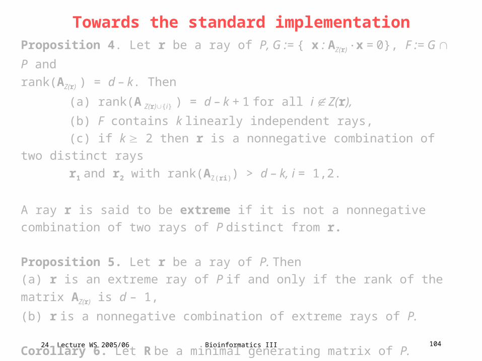
Towards the standard implementationProposition 4. Let r be a ray of P, G := { x : AZ(r) x = 0}, F := G P and
rank(AZ(r) ) = d – k. Then
(a) rank(A Z(r){i} ) = d – k + 1 for all i Z(r),
(b) F contains k linearly independent rays,
(c) if k 2 then r is a nonnegative combination of two distinct rays
r1 and r2 with rank(AZ(ri)) > d – k, i = 1,2.
A ray r is said to be extreme if it is not a nonnegative combination of two rays of P
distinct from r.
Proposition 5. Let r be a ray of P. Then
(a) r is an extreme ray of P if and only if the rank of the matrix AZ(r) is d – 1,
(b) r is a nonnegative combination of extreme rays of P.
Corollary 6. Let R be a minimal generating matrix of P.
Then R is the set of extreme rays of P.

24. Lecture WS 2005/06
Bioinformatics III 105
Towards the standard implementationTwo distinct extreme rays r and r‘ of P are adjacent if the minimal face of P
containing both contains no other extreme rays.
Proposition 7. Let r and r‘ be distinct rays of P.
Then the following statements are equivalent
(a) r and r‘ are adjacent extreme rays,
(b) r and r‘ are extreme rays and the rank of the matrix AZ(r) Z(r‘) is d – 2,
(c) if r‘‘ is a ray with Z(r‘‘) Z(r) Z(r‘) then either r‘‘ ≃ r or r‘‘ ≃ r.
Lemma 8. Let (AK,R) be a DD pair such than rank(AK) = d and let i be a row index
of A not in K. Then the pair (AK+i , R‘) is a DD pair, where R‘ is the d | J‘| matrix
with column vectors rj (j J‘) defined by
J‘ = J+ J0 Adj
Adj = {(j,j‘) J+ J- : rj and rj‘ are adjacent in P(AK)} and
r = (Ai rj ) rj‘ – (Airj ) rj for each (j,j‘) Adj.
Furthermore, if R is a minimal generating matrix for P(AK) then R‘ is a minimal
generating matrix for P(AK+i).

24. Lecture WS 2005/06
Bioinformatics III 106
Algorithm for standard form of double description methodHence we can write a straightforward variation of the DD method which produces
a minimal generating set for P:
To implement DDMethodStandard, we must check for each pair of extreme rays
r and r‘ of P(AK) with Ai r > 0 and Ai r‘ < 0 whether they are adjacent in P(AK).
As stated in Proposition 7, there are two ways to check adjacency, the
combinatiorial and the algebraic way. While it cannot be rigorously shown which
method is more efficient, in practice, the combinatorial method is always faster.
DDMethodStandard(A)
such that R is minimal
Lemma 8
Q: Describe briefly the strategy of the double decomposition method.What is the connection to the algorithm to compute extreme pathways?

24. Lecture WS 2005/06
Bioinformatics III 107
V21 Current metabolomicsReview:
(1) recent work on metabolic networks required revising the picture of separate
biochemical pathways into a densely-woven metabolic network
(2) The connectivity of substrates in this network follows a power-law.
(3) Constraint-based modeling approaches (FBA) were successful in analyzing the
capabilities of cellular metabolism including
- its capacity to predict deletion phenotypes
- the ability to calculate the relative flux values of metabolic reactions, and
- the capability to identify properties of alternate optimal growth states
in a wide range of simulated environmental conditions
Open questions
- what parts of metabolism are involved in adaptation to environmental conditions?
- is there a central essential metabolic core?
- what role does transcriptional regulation play?

24. Lecture WS 2005/06
Bioinformatics III 108
Distribution of fluxes in E.coli
Stoichiometric matrix for E.coli strain MG1655 containing 537 metabolites and
739 reactions taken from Palsson et al.
Apply flux balance analysis to characterize solution space
(all possible flux states under a given condition).
Nature 427, 839 (2004)
Aim: understand principles that govern
the use of individual reactions under
different growth conditions.
j
jiji vSAdt
d0
vj is the flux of reaction j and Sij is the stoichiometric coefficient of reaction j.

24. Lecture WS 2005/06
Bioinformatics III 109
Optimal states
Using linear programming and adapting constraints for each reaction flux vi of the
form imin ≤ vi ≤ i
max, the flux states were calculated that optimize cell growth on
various substrates.
Plot the flux distribution for active (non-zero flux) reactions of E.coli grown in a
glutamate- or succinate-rich substrate.
Denote the mass carried by reaction j producing (consuming) metabolite i by
Fluxes vary widely: e.g. dimensionless flux of succinyl coenzyme A synthetase
reaction is 0.185, whereas the flux of the aspartate oxidase reaction is 10.000
times smaller, 2.2 10-5.
jijij vSv ˆ

24. Lecture WS 2005/06
Bioinformatics III 110
Overall flux organization of E.coli metabolic network
a, Flux distribution for optimized biomass production
on succinate (black) and glutamate (red) substrates.
The solid line corresponds to the power-law fit
that a reaction has flux v
P(v) (v + v0)- , with v0 = 0.0003 and = 1.5.
d, The distribution of experimentally determined fluxes
from the central metabolism of E. coli shows
power-law behaviour as well, with a best fit to
P(v) v- with = 1.
Both computed and experimental flux distribution
show wide spectrum of fluxes.
Almaar et al., Nature 427, 839 (2004)

24. Lecture WS 2005/06
Bioinformatics III 111
Use scaling behavior to determine local connectivity
The observed flux distribution is compatible with two different potential local
flux structures:
(a) a homogenous local organization would imply that all reactions producing
(consuming) a given metabolite have comparable fluxes
(b) a more delocalized „high-flux backbone (HFB)“ is expected if the local flux
organisation is heterogenous such that each metabolite has a dominant
source (consuming) reaction.
Schematic illustration of the hypothetical scenario in which
(a) all fluxes have comparable activity, in which case we expect kY(k) 1 and
(b) the majority of the flux is carried by a single incoming or outgoing reaction,
for which we should have kY(k) k . Almaar et al., Nature 427, 839 (2004)

24. Lecture WS 2005/06
Bioinformatics III 112
Measuring the importance of individual reactions
To distinguish between these 2 schemes for each metabolite i produced
(consumed) by k reactions, define
Almaar et al., Nature 427, 839 (2004)
2
11ˆ
ˆ,
k
jk
l ilv
ijv
ikY
where vij is the mass carried by reaction j which produces (consumes) metabolite i.
If all reactions producing (consuming) metabolite i have comparable vij
values, Y(k,i) scales as 1/k.
If, however, the activity of a single reaction dominates we expect
Y(k,i) 1 (independent of k).

24. Lecture WS 2005/06
Bioinformatics III 113
Characterizing the local inhomogeneity of the flux net
a, Measured kY(k) shown as a function of k for
incoming and outgoing reactions, averaged over
all metabolites, indicates that Y(k) k-0.27.
Inset shows non-zero mass flows, v^ij, producing
(consuming) FAD on a glutamate-rich substrate.
an intermediate behavior is found between the
two extreme cases.
the large-scale inhomogeneity observed in the
overall flux distribution is also increasingly valid at
the level of the individual metabolites.
The more reactions that consume (produce) a
given metabolite, the more likely it is that a single
reaction carries most of the flux, see FAD.
Almaar et al., Nature 427, 839 (2004)

24. Lecture WS 2005/06
Bioinformatics III 114
Clean up metabolic network
Simple algorithm removes for each metabolite systematically all reactions
but the one providing the largest incoming (outgoing) flux distribution.
The algorithm uncovers the „high-flux-backbone“ of the metabolism,
a distinct structure of linked reactions that form a giant component
with a star-like topology.
Almaar et al., Nature 427, 839 (2004)

24. Lecture WS 2005/06
Bioinformatics III 115
FBA-optimized network on glutamate-rich substrateHigh-flux backbone for FBA-optimized metabolic
network of E. coli on a glutamate-rich substrate.
Metabolites (vertices) coloured blue have at least one
neighbour in common in glutamate- and succinate-rich
substrates, and those coloured red have none.
Reactions (lines) are coloured blue if they are identical
in glutamate- and succinate-rich substrates, green if a
different reaction connects the same neighbour pair,
and red if this is a new neighbour pair. Black dotted
lines indicate where the disconnected pathways, for
example, folate biosynthesis, would connect to the
cluster through a link that is not part of the HFB. Thus,
the red nodes and links highlight the predicted changes
in the HFB when shifting E. coli from glutamate- to
succinate-rich media. Dashed lines indicate links to the
biomass growth reaction.
Almaar et al., Nature 427, 839 (2004)
(1) Pentose Phospate (11) Respiration
(2) Purine Biosynthesis (12) Glutamate Biosynthesis (20) Histidine Biosynthesis
(3) Aromatic Amino Acids (13) NAD Biosynthesis (21) Pyrimidine Biosynthesis
(4) Folate Biosynthesis (14) Threonine, Lysine and Methionine Biosynthesis
(5) Serine Biosynthesis (15) Branched Chain Amino Acid Biosynthesis
(6) Cysteine Biosynthesis (16) Spermidine Biosynthesis (22) Membrane Lipid Biosynthesis
(7) Riboflavin Biosynthesis (17) Salvage Pathways (23) Arginine Biosynthesis
(8) Vitamin B6 Biosynthesis (18) Murein Biosynthesis (24) Pyruvate Metabolism
(9) Coenzyme A Biosynthesis (19) Cell Envelope Biosynthesis (25) Glycolysis
(10) TCA Cycle

24. Lecture WS 2005/06
Bioinformatics III 116
Interpretation
Only a few pathways appear disconnected indicating that although these pathways
are part of the HFB, their end product is only the second-most important source for
another HFB metabolite.
Groups of individual HFB reactions largely overlap with traditional biochemical
partitioning of cellular metabolism.
Almaar et al., Nature 427, 839 (2004)
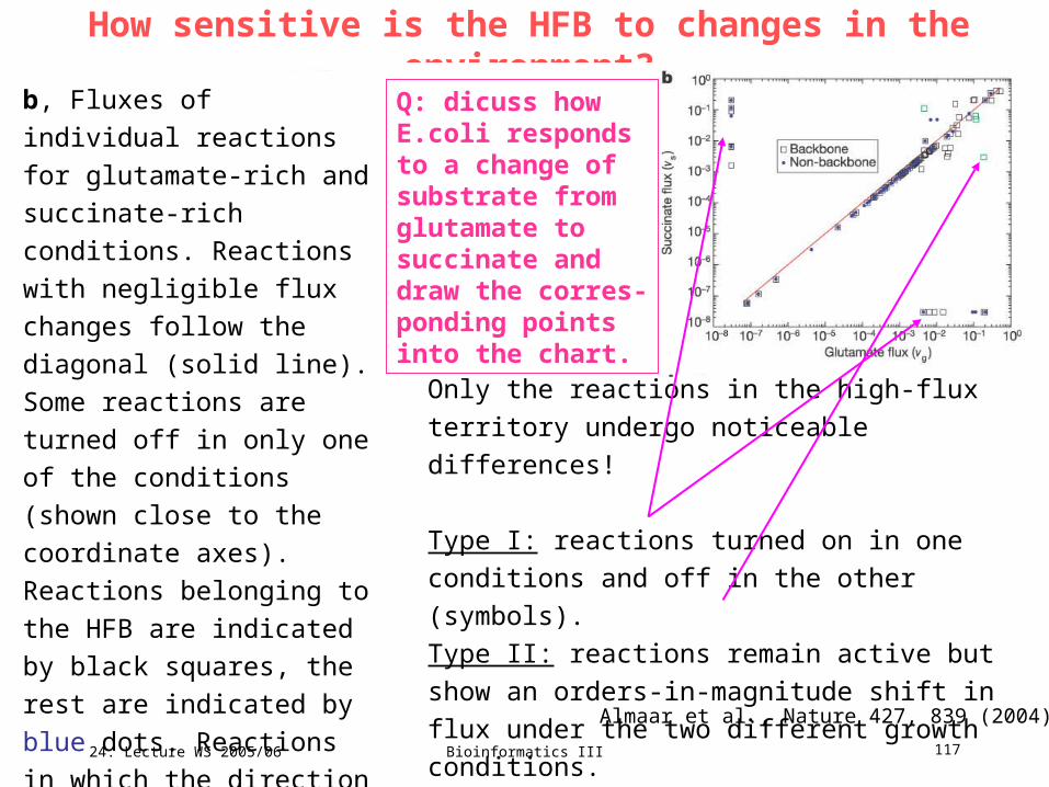
24. Lecture WS 2005/06
Bioinformatics III 117
How sensitive is the HFB to changes in the environment?
Almaar et al., Nature 427, 839 (2004)
b, Fluxes of individual
reactions for glutamate-rich
and succinate-rich conditions.
Reactions with negligible flux
changes follow the diagonal
(solid line).
Some reactions are turned off
in only one of the conditions
(shown close to the
coordinate axes). Reactions
belonging to the HFB are
indicated by black squares,
the rest are indicated by blue
dots. Reactions in which the
direction of the flux is
reversed are coloured green.
Only the reactions in the high-flux territory
undergo noticeable differences!
Type I: reactions turned on in one conditions and
off in the other (symbols).
Type II: reactions remain active but show an
orders-in-magnitude shift in flux under the two
different growth conditions.
Q: dicuss how E.coli respondsto a change of substrate fromglutamate to succinate anddraw the corres-ponding pointsinto the chart.

24. Lecture WS 2005/06
Bioinformatics III 118
Flux distributions for individual reactions
Shown is the flux distribution for four selected
E. coli reactions in a 50% random environment.
a Triosphosphate isomerase;
b carbon dioxide transport;
c NAD kinase;
d guanosine kinase.
Reactions on the v curve (small fluxes)
have unimodal/gaussian distributions (a and
c). Shifts in growth-conditions only lead to small
changes of their flux values.
Reactions off this curve have multimodal
distributions (b and d), showing several
discrete flux values under diverse conditions.
Under different growth conditions they show
several discrete and distinct flux values.
Almaar et al., Nature 427, 839 (2004)
24. Lecture WS 2005/06
Bioinformatics III 119
Summary Metabolic network use is highly uneven (power-law distribution) at the global level
and at the level of the individual metabolites.
Whereas most metabolic reactions have low fluxes, the overall activity of the
metabolism is dominated by several reactions with very high fluxes.
E. coli responds to changes in growth conditions by reorganizing the rates of
selected fluxes predominantly within this high-flux backbone.
Apart from minor changes, the use of the other pathways remains unaltered.
These reorganizations result in large, discrete changes in the fluxes of the HFB
reactions.

24. Lecture WS 2005/06
Bioinformatics III 120
The same authors as before used Flux Balance Analysis to examine utilization
and relative flux rate of each metabolite in a wide range of simulated
environmental conditions for E.coli, H. pylori and S. cerevisae:
consider in each case 30.000 randomly chosen combinations where each uptake
reaction is a assigned a random value between 0 and 20 mmol/g/h.
adaptation to different conditions occurs by 2 mechanisms:
(a) flux plasticity: changes in the fluxes of already active reactions.
E.g. changing from glucose- to succinate-rich conditions alters the flux of 264
E.coli reactions by more than 20%
(b) less commonly, adaptation includes structural plasticity, turning on
previously zero-flux reactions or switching off active pathways.

24. Lecture WS 2005/06
Bioinformatics III 121
The two adaptation method mechanisms allow for the possibility of a group of
reactions not subject to structural plasticity being active under all environmental
conditions.
Assume that active reactions were randomly distributed.
If typically a q fraction of the metabolic reactions are active under a specific
growth condition,
we expect for n distinct conditions an overlap of at least qn reactions.
This converges quickly to 0.
Emergence of the Metabolic Core

24. Lecture WS 2005/06
Bioinformatics III 122
However, as the number of conditions increases, the curve converges to a
constant enoted by the dashed line, identifying the metabolic core of an organism.
Red line : number of reactions that are always active if activity is randomly
distributed in the metabolic network. The fact that it converges to zero indicates
that the real core represents a collective network effect, forcing a group of
reactions to be active in all conditions.
Emergence of the Metabolic Core(A–C) The average relative size of the number of reactions that are always active as a function of the number of sampled conditions (blackline) for (A) H. pylori, (B) E. coli, and (C) S. cerevisiae.(D and E) The number of metabolic reactions (D) and the number of metabolic core reactions (E) in the three studied organisms.
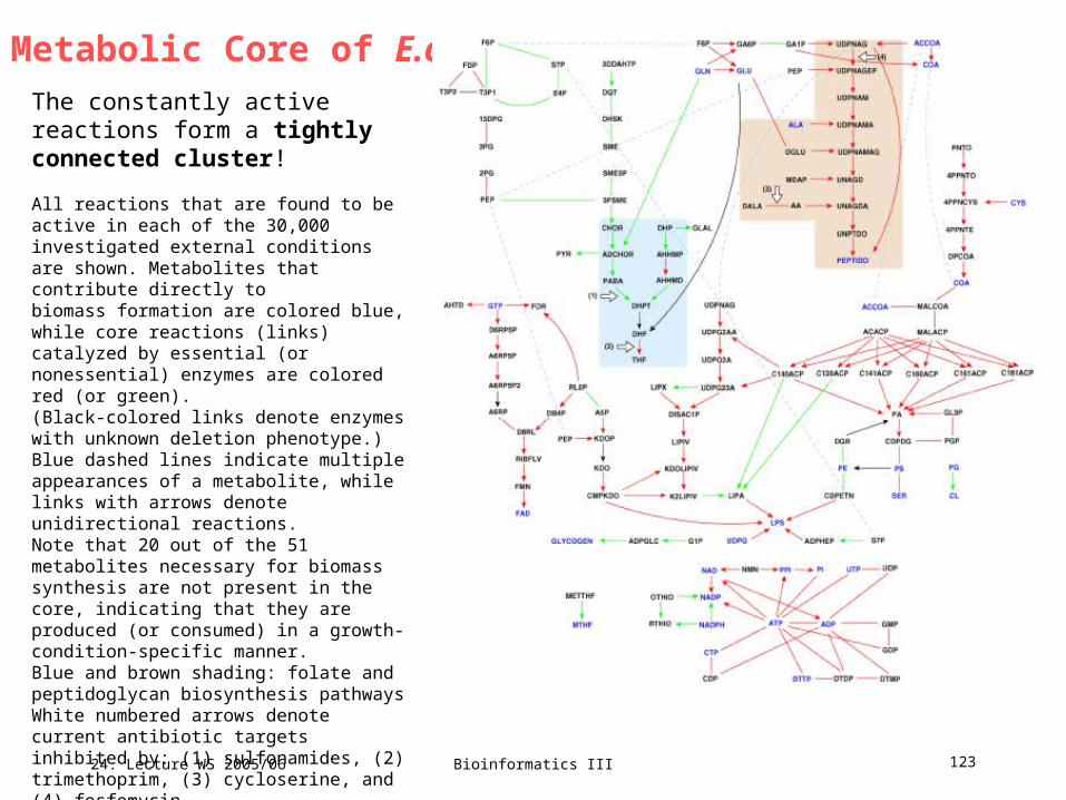
24. Lecture WS 2005/06
Bioinformatics III 123
The constantly active reactions form a tightly connected cluster!
All reactions that are found to be active in each of the 30,000 investigated external conditions are shown. Metabolites that contribute directly tobiomass formation are colored blue, while core reactions (links) catalyzed by essential (or nonessential) enzymes are colored red (or green).(Black-colored links denote enzymes with unknown deletion phenotype.) Blue dashed lines indicate multiple appearances of a metabolite, while links with arrows denote unidirectional reactions. Note that 20 out of the 51 metabolites necessary for biomass synthesis are not present in the core, indicating that they are produced (or consumed) in a growth-condition-specific manner. Blue and brown shading: folate and peptidoglycan biosynthesis pathways White numbered arrows denote current antibiotic targets inhibited by: (1) sulfonamides, (2) trimethoprim, (3) cycloserine, and (4) fosfomycin. A few reactions appear disconnected since we have omitted the drawing of cofactors.
Metabolic Core of E.coli

24. Lecture WS 2005/06
Bioinformatics III 124
The metabolic cores contain 2 types of reactions:
(a) reactions that are essential for biomass production under all environment
conditions (81 of 90 in E.coli)
(b) reactions that assure optimal metabolic performance.
Metabolic Core Reactions

24. Lecture WS 2005/06
Bioinformatics III 125
(A) The number of overlapping metabolic reactions in the
metabolic core of H. pylori, E. coli, and S. cerevisiae.
The metabolic cores of simple organisms (H. pylori and
E.coli) overlap to a large extent.
The largest organism (S.cerevisae) has a much larger
reaction network that allows more flexbility the relative
size of the metabolic core is much lower.
(B) The fraction of metabolic reactions catalyzed by
essential enzymes in the cores (black) and outside the
core in E. coli and S. cerevisiae.
Reactions of the metabolic core are mostly
essential ones.
(C) One could assume that the core represents a subset
of high-flux reactions. This is apparently not the case.
The distributions of average metabolic fluxes for the
core and the noncore reactions in E. coli are very
similar.
Characterizing the Metabolic Cores
24. Lecture WS 2005/06
Bioinformatics III 126
- Adaptation to environmental conditions occurs via structural plasticity and/or flux
plasticity.
Here: identification of a surprisingly stable metabolic core of reactions that are
tightly connected to eachother.
- the reactions belonging to this core represent potential targets for antimicrobial
intervention.
Summary
24. Lecture WS 2005/06
Bioinformatics III 127
Integrated Analysis of Metabolic and Regulatory Networksis omitted ...

24. Lecture WS 2005/06
Bioinformatics III 128
V22 Modelling Dynamic Cellular Processes
John Tyson Bela Novak
Mathematical description of signalling
pathways helps answering questions like:
(1) How do the magnitudes of signal output
and signal duration depend on the kinetic
properties of pathway components?
(2) Can high signal amplification be coupled
with fast signaling?
(3) How are signaling pathways designed to
ensure that they are safely off in the absence
of stimulation, yet display high signal
amplification following receptor activation?
(4) How can different agonists stimulate the
same pathway in distinct ways to elicit a
sustained or a transient response, which can
have dramatically different consequences?
Heinrich et al. Mol. Cell. 9, 957 (2002)

24. Lecture WS 2005/06
Bioinformatics III 129
Protein synthesis and degradation: linear response
RkSkkdt
dR210
S = signal strength (e.g. concentration of mRNA)
R = response magnitude (e.g. concentration of protein)
Tyson et al., Curr.Pin.Cell.Biol. 15, 221 (2003)
A steady-state solution of a differential equation, dR/dt = f(R) is a constant Rss
that satisfies the algebraic equation f(Rss) = 0. In this case
2
10
k
SkkR
ss

24. Lecture WS 2005/06
Bioinformatics III 130
Protein synthesis and degradation
RkSkkdt
dR210
Tyson et al., Curr.Pin.Cell.Biol. 15, 221 (2003)
Solid curve: rate of removal of the
response component R.
Dashed lines: rates of production of R
for various values of signal strength.
Filled circles: steady-state solutions
where rate of production and rate of
removal are identical.
Wiring diagram rate curve signal-response curve
Steady-state response R as a
function of signal strength S.
2
10
k
SkkR
ss
Parameters:k0 = 0.01k1 = 1k2 = 5

24. Lecture WS 2005/06
Bioinformatics III 131
phosphorylation/dephosphorylation: hyperbolic response
Tyson et al., Curr.Pin.Cell.Biol. 15, 221 (2003)
TP
PPTP
PPPT
SRkSkkR
SRkSRkSRkRk
RkRkRRSk
112
1112
2210
A steady-state solution:
Skk
SRR T
ssP
12
,
PPT
P RkRRSkdt
dR21
RP: phosphorylated form of the response element
RP= [RP]
Pi: inorganic phosphate
RT = R + RP total concentration of R
Parameters:k1 = k2 = 1RT = 1
Q: the time-dependenceof RP is given.Derive the steady-stateconcentration RP,ss.

24. Lecture WS 2005/06
Bioinformatics III 132
phosphorylation/dephosphorylation: sigmoidal response
Tyson et al., Curr.Pin.Cell.Biol. 15, 221 (2003)
Modification of (b) where the phosphorylation and
dephosphorylation are governed by Michaelis-
Menten kinetics:
Pm
P
PTm
PTP
RK
Rk
RRK
RRSk
dt
dR
2
2
1
1
PmPTPTmP
PTm
PT
Pm
P
Pm
P
PTm
PT
RKRRSkRRKRk
RRK
RRSk
RK
Rk
RK
Rk
RRK
RRSk
2112
1
1
2
2
2
2
1
10
steady-state solution of RP The biophysically acceptable solutions
must be in the range 0 < RP < RT:
T
m
T
m
T
ssP
R
K
R
KkSkG
R
R21
21
, ,,,
with the „Goldbeter-Koshland“ function G:
uKuvuKvJuvuKvJuv
uK
KJvuG
4
2
),,,(
2

24. Lecture WS 2005/06
Bioinformatics III 133
phosphorylation/dephosphorylation: sigmoidal response
This mechanism creates a switch-like signal-response curve which is
called zero-order ultrasensitivity.
(a), (b), and (c) give „graded“ and reversible behavior of R and S.
„graded“: R increases continuously with S
reversible: if S is change from Sinitial to Sfinal , the response at Sfinal is the same
whether the signal is being increased (Sinitial < Sfinal) or decreased (Sinitial > Sfinal).
Element behaves like a buzzer: to activate the response, one must push hard
enough on the button.Tyson et al., Curr.Pin.Cell.Biol. 15, 221 (2003)
Parameters:k1 = k2 = 1RT = 1Km1 = Km2 = 0.05

24. Lecture WS 2005/06
Bioinformatics III 134
perfect adaptation: sniffer
Tyson et al., Curr.Pin.Cell.Biol. 15, 221 (2003)
Here, the simple linear response element is supplemented
with a second signaling pathway through species X.
XkSkdt
dX
RXkSkdt
dR
43
21
32
41
2
1
4
3
kk
kk
Xk
SkR
k
SkX
ss
ss
The response mechanism exhibits perfect adaptation to the signal:
although the signaling pathway exhibits a transient response to changes in signal
strength, its steady-state response Rss is independent of S.
Such behavior is typical of chemotactic systems, which respond to an abrupt
change in attractants or repellents, but then adapt to a constant level of the signal.
Our own sense of smell operates this way we call this element „sniffer“.
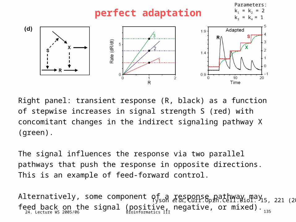
24. Lecture WS 2005/06
Bioinformatics III 135
perfect adaptation
Right panel: transient response (R, black) as a function of stepwise increases
in signal strength S (red) with concomitant changes in the indirect signaling
pathway X (green).
The signal influences the response via two parallel pathways that push the
response in opposite directions. This is an example of feed-forward control.
Alternatively, some component of a response pathway may feed back on the
signal (positive, negative, or mixed).
Tyson et al., Curr.Opin.Cell.Biol. 15, 221 (2003)
Parameters:k1 = k2 = 2k3 = k4 = 1

24. Lecture WS 2005/06
Bioinformatics III 136
Positive feedback: Mutual activation
Tyson et al., Curr.Opin.Cell.Biol. 15, 221 (2003)
E: a protein involved with R
EP: phosphorylated form of E
Here, R activates E by phosphorylation,
and EP enhances the synthesis of R.
4343
210
,,, JJkRkGRE
RkSkREkdt
dR
P
P

24. Lecture WS 2005/06
Bioinformatics III 137
mutual activation: one-way switch
As S increases, the response is low until S exceeds a critical value Scrit at which
point the response increases abruptly to a high value.
Then, if S decreases, the response stays high.
between 0 and Scrit, the control system is „bistable“ – it has two stable
steady-state response values (on the upper and lower branches, the solid lines)
separated by an unstable steady state (on the intermediate branch, the dashed
line).
This is called a one-parameter bifurcation. Tyson et al., Curr.Opin.Cell.Biol. 15, 221 (2003)

24. Lecture WS 2005/06
Bioinformatics III 138
Negative feedback: homeostasis
Tyson et al., Curr.Opin.Cell.Biol. 15, 221 (2003)
In negative feedback, the response counteracts the effect of the stimulus.
Here, the response element R inhibits the enzyme E catalyzing its synthesis.
Therefore, the rate of production of R is a sigmoidal decreasing function of R.
4343
20
,,, JJRkkGRE
RSkREkdt
dR
Negative feedback in a two-component
system X R | X can also exhibit
damped oscillations to a stable steady state
but not sustained oscillations.

24. Lecture WS 2005/06
Bioinformatics III 139
Negative feedback: oscillatory response
Tyson et al., Curr.Opin.Cell.Biol. 15, 221 (2003)
There are two ways to close the negative feedback loop:
(1) RP inhibits the synthesis of X
(2) RP activates the degradation of X.
Sustained oscillations require at least 3 components:
X Y R |X
Left: example for a negative-feedback control loop.
Pm
P
PTm
PTPP
Pm
P
PTm
PTP
P
RK
Rk
RRK
RRYk
dt
dR
YK
Yk
YYK
YYXk
dt
dY
XRkXkSkkdt
dX
6
6
5
5
4
4
3
3
'
2210
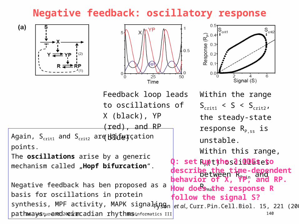
24. Lecture WS 2005/06
Bioinformatics III 140
Negative feedback: oscillatory response
Feedback loop leads to
oscillations of X (black),
YP (red), and RP (blue).
Tyson et al., Curr.Pin.Cell.Biol. 15, 221 (2003)
Within the range Scrit1 < S
< Scrit2, the steady-state
response RP,ss is unstable.
Within this range, RP(t)
oscillates between RPmin
and RPmax.
Again, Scrit1 and Scrit2 are bifurcation points.
The oscillations arise by a generic mechanism
called „Hopf bifurcation“.
Negative feedback has ben proposed as a basis for
oscillations in protein synthesis, MPF activity, MAPK
signaling pathways, and circadian rhythms.
Q: set up the 3 ODEs to describe the time-dependentbehavior of X, YP, and RP.How does the response Rfollow the signal S?

24. Lecture WS 2005/06
Bioinformatics III 141
Positive and negative feedback: Activator-inhibitor oscillations
R is created in an autocatalytic
process, and then promotes the
production of an inhibitor X,
which speeds up R removal.
Tyson et al., Curr.Pin.Cell.Biol. 15, 221 (2003)
4343
65
'
2210
,,, JJkRkGRE
XkRkdt
dX
RXkRkSkREkdt
dR
P
P
The classic example of such a system is cyclic AMP production in the slime mold. External cAMP binds to a surface receptor, which stimulates adenylate cyclase to produce and excrete more cAMP. At the same time, cAMP-bindingpushes the receptor into an inactive form. After cAMP falls off, the inactive form slowly recovers its ability tobind cAMP and stimulate adenylate cyclase again.

24. Lecture WS 2005/06
Bioinformatics III 142
V23 Stochastic simulations of cellular signalling
Traditional computational approach to chemical/biochemical kinetics:
(a) start with a set of coupled ODEs (reaction rate equations) that describe the
time-dependent concentration of chemical species,
(b) use some integrator to calculate the concentrations as a function of time given
the rate constants and a set of initial concentrations.
Successful applications : studies of yeast cell cycle, metabolic engineering,
whole-cell scale models of metabolic pathways (E-cell), ...
Major problem: cellular processes occur in very small volumes and
frequently involve very small number of molecules.
E.g. in gene expression processes a few TF molecules may interact with a
single gene regulatory region.
E.coli cells contain on average only 10 molecules of Lac repressor.

24. Lecture WS 2005/06
Bioinformatics III 143
Include stochastic effects
(Consequence1) modeling of reactions as continuous fluxes of matter is no
longer correct.
(Consequence2) Significant stochastic fluctuations occur.
To study the stochastic effects in biochemical reactions stochastic formulations of
chemical kinetics and Monte Carlo computer simulations have been used.
Daniel Gillespie (J Comput Phys 22, 403 (1976); J Chem Phys 81, 2340 (1977))
introduced the exact Dynamic Monte Carlo (DMC) method that connects the
traditional chemical kinetics and stochastic approaches.
Assuming that the system is well mixed, the rate constants appearing in these two
methods are related.

24. Lecture WS 2005/06
Bioinformatics III 144
Dynamic Monte Carlo
In the usual implementation of DMC for kinetic simulations, each reaction is
considered as an event and each event has an associated probability of occurring.
The probability P(Ei) that a certain chemical reaction Ei takes place in a given time
interval t is proportional to an effective rate constant k and to the number of
chemical species that can take part in that event.
E.g. the probability of the first-order reaction
X Y + Z
would be k1Nx with Nx :number of species X, and
k1 : rate constant of the reaction
Similarly, the probability of the reverse second-order reaction
Y + Z X
would be k2NYNZ.
Resat et al., J.Phys.Chem. B 105, 11026 (2001)

24. Lecture WS 2005/06
Bioinformatics III 145
Dynamic Monte Carlo
As the method is a probabilistic approach based on „events“, „reactions“ included in
the DMC simulations do not have to be solely chemical reactions.
Any process that can be associated with a probability can be included as an event
in the DMC simulations.
E.g. a substrate attaching to a solid surface can initiate a series of chemical
reactions.
One can split the modelling into the physical events of substrate arrival, of
attaching the substrate, followed by the chemical reaction steps.
Resat et al., J.Phys.Chem. B 105, 11026 (2001)

24. Lecture WS 2005/06
Bioinformatics III 146
Basic outline of the direct method of Gillespie
(Step i) generate a list of the components/species and define the initial distribution
at time t = 0.
(Step ii) generate a list of possible events Ei (chemical reactions as well as
physical processes).
(Step iii) using the current component/species distribution, prepare a probability
table P(Ei) of all the events that can take place.
Compute the total probability
P(Ei) : probability of event Ei .
(Step iv) Pick two random numbers r1 and r2 [0...1] to decide which event E will
occur next and the amount of time by which E occurs later since the most recent
event.
Resat et al., J.Phys.Chem. B 105, 11026 (2001)
)(itotEPP

24. Lecture WS 2005/06
Bioinformatics III 147
Basic outline of the direct method of Gillespie
Using the random number r1 and the probability table,
the event E is determined by finding the event that satisfies the relation
Resat et al., J.Phys.Chem. B 105, 11026 (2001)
1
1
11
ii
itoti
EPPrEP
The second random number r2 is used to obtain the amount of time between the
reactions
2ln
1r
Ptot
As the total probability of the events changes in time, the time step between
occurring steps varies.
Steps (iii) and (iv) are repeated at each step of the simulation.
The necessary number of runs depends on the inherent noise of the system and on
the desired statistical accuracy.
weighted sampling (PW-DMC) is omitted.