TECHNISCHE MECHANIK, Band 29, Heft 1, (2009), 1 – 12Manuskripteingang: 19. November 2007

The Simplest Model of the Turning Movement of a Car with its PossibleSideslip

A.B. Byachkov, C. Cattani, E.M. Nosova, M.P. Yushkov

The simplest model of the turning movement of a car with its possiple sideslip is considered. To this end, a non-holonomic problem with nonretaining constraints is solved. The four possible types of the car motion are studied.

1 Problem Formulation

The complete theory of the motion of a car with deformable wheels has been developed by N. A. Fufaev anddetailed in his book (1989). The treatise by V. F. Zhuravlev and N. A. Fufaev (1993) is devoted to mechanics ofsystems with nonretaining constraints. In this treatise the Boltzmann-Hamel equations are used for studying themotion of nonholonomic systems; and the possibility of restoring nonholonomic constraints is investigated onthe basis of behaviour of solution curves in the common space of generalized coordinates and quasivelocities.In this work the Maggi equations, which make it possible to easily determine the generalized reaction forcesof nonholonomic constraints, are applied (Zegzhda et al., 2005); the beginning and stop of wheels sideslip isdetermined by these constraint forces.

In the paper (Sheverdin and Yushkov, 2002) the Maggi equations have been formed for studying the simplest modelof the motion of a car while turning (see Figure 1). The car is assumed to consist of the body of mass M1 andthe front axle of mass M2. They have moments of inertia J1 and J2, respectively, about the vertical axes thatgo through their centers of mass. The front axle can rotate about its vertical axis going through the axle’s center.Masses of the wheels and back axle as separate parts are neglected. This scheme requires introduction of fourgeneralized coordinates: q1 = ϕ, q2 = θ, q3 = ξC , and q4 = ηC . The car is driven by a force F1(t) actingalong its longitudinal axis and moment L1(t) turning the front axle, F1(t), L1(t) being given functions of time.Besides these, a resisting force F2(vC) acting in the direction opposite to the direction of the velocity vC of thecar body centre of mass C, resisting moment L2(θ) applied to the front axle and opposite to the angular velocityof its rotation, and restoring moment L3(θ) are taken into account. A similar scheme is introduced in (Lineikin,1939) as a simplified mathematical model of the motion of a car while turning. In this formulation, the turningmovement of a car is studied, figuratively speaking, under ”dynamical control”, when the turning moment L1(t),resisting moment L2(θ), and restoring moment L3(θ) are applied to the rotating front axle. When introducing twononholonomic constraints corresponding to the absence of side slipping of the back and front axles of the car (theirequations (1) and (2) are given below), two Maggi’s equations had to be set up.

Now consider the ”kinematic control”, under which the turning of the front axle is determined by a driver as acertain time function θ = θ(t). In this scheme a turning car has three degrees of freedom: q1 = ϕ, q2 = ξC ,q3 = ηC . The varying function θ = θ(t) characterizes only nonstationarity of the problem. As this takes place,nonholonomic constraints

ϕ1 ≡ −ξC sin ϕ + ηC cosϕ− l2ϕ = 0 (1)

ϕ2 ≡ −ξC sin(ϕ + θ) + ηC cos(ϕ + θ) + l1ϕ cos θ = 0 (2)

should be satisfied by the car motion (these equations are derived in detail in the treatise (Zegzhda et al., 2005)).We consider these constraints as nonretaining. The active forces F1(t) and F2(t) have the same meaning as in thework (Sheverdin and Yushkov, 2002).

1

2 The Turning Movement of a Car with Retaining (bilateral) Constraints

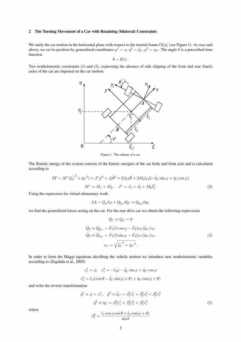
We study the car motion in the horizontal plane with respect to the inertial frame Oξηζ (see Figure 1). As was saidabove, we set its position by generalized coordinates q1 = ϕ, q2 = ξC , q3 = ηC . The angle θ is a prescribed timefunction

θ = θ(t) .

Two nonholonomic constraints (1) and (2), expressing the absence of side slipping of the front and rear (back)axles of the car are imposed on the car motion.

Figure 1. The scheme of a car.

The Kinetic energy of the system consists of the kinetic energies of the car body and front axle and is calculatedaccording to

2T = M∗( ˙ξC2

+ ˙ηC2) + J∗ϕ2 + J2θ

2 + 2J2ϕθ + 2M2l1ϕ(−ξC sin ϕ + ηC cos ϕ)

M∗ = M1 + M2, J∗ = J1 + J2 + M2l21 . (3)

Using the expression for virtual elementary work

δA = Qϕδϕ + QξCδξC + QηC

δηC

we find the generalized forces acting on the car. For the rear drive car we obtain the following expressions

Q1 ≡ Qϕ = 0

Q2 ≡ QξC= F1(t) cos ϕ− F2(vC)ξC/vC

Q3 ≡ QηC = F1(t) sin ϕ− F2(vC)ηC/vC (4)

vC =√

˙ξC2

+ ˙ηC2 .

In order to form the Maggi equations decribing the vehicle motion we introduce new nonholonomic variablesaccording to (Zegzhda et al., 2005)

v1∗ = ϕ, v2

∗ = −l2ϕ− ξC sin ϕ + ηC cosϕ

v3∗ = l1ϕ cos θ − ξC sin(ϕ + θ) + ηC cos(ϕ + θ)

and write the reverse transformation

q1 ≡ ϕ = v1∗ , q2 ≡ ξC = β2

1v1∗ + β2

2v2∗ + β2

3v3∗

q3 ≡ ηC = β31v1∗ + β3

2v2∗ + β3

3v3∗ (5)

where

β21 =

l1 cos ϕ cos θ + l2 cos(ϕ + θ)sin θ

2

β22 =

cos(ϕ + θ)sin θ

, β23 = −cosϕ

sin θ(6)

β31 =

l1 sin ϕ cos θ + l2 sin(ϕ + θ)sin θ

β32 =

sin(ϕ + θ)sin θ

, β33 = − sin ϕ

sin θ.

The first group of the Maggi equations in this case consists of one equation

(MW1 −Q1)∂q1

∂v1∗+ (MW2 −Q2)

∂q2

∂v1∗+ (MW3 −Q3)

∂q3

∂v1∗= 0 . (7)

The expressions MWσ can be calculated using kinetic energy by the formulas

MWσ =d

dt

∂T

∂qσ− ∂T

∂qσ, σ = 1, 3 .

Consequently, using expressions (3), (4), (5), (6), let us represent the motion equation (7) in the following expandedform

J∗ϕ + J2θ + M2l1(−ξC sinϕ + ηC cosϕ)+

+β21(M∗ξC −M2l1(ϕ sin ϕ + ϕ2 cos ϕ)− F1(t) cos ϕ + F2(vC)ξC/vC)+ (8)

+β31(M∗ηC + M2l1(ϕ cosϕ− ϕ2 sin ϕ)− F1(t) sin ϕ + F2(vC)ηC/vC) = 0 .

The equations of constraints (1) and (2) should be added to this equation.

If the initial conditions and analytic representation of the functions F1(t), F2(vC) are given, then after numericalintegration of the nonlinear system of differential equations (1), (2), (8) we find the car motion

ϕ = ϕ(t), ξC = ξC(t), ηC = ηC(t). (9)

Now we can determine the generalized reaction forces Λ1, Λ2. The second group of Maggi’s equations will bewritten as follows

Λ1 = (MW1 −Q1)∂q1

∂v2∗+ (MW2 −Q2)

∂q2

∂v2∗+ (MW3 −Q3)

∂q3

∂v2∗

Λ2 = (MW1 −Q1)∂q1

∂v3∗+ (MW2 −Q2)

∂q2

∂v3∗+ (MW3 −Q3)

∂q3

∂v3∗or in the extended form for the rear drive vehicle

Λ1 = β22(M∗ξC −M2l1(ϕ sin ϕ + ϕ2 cos ϕ)− F1(t) cos ϕ + F2(vC)ξC/vC)+

+β32(M∗ηC + M2l1(ϕ cosϕ− ϕ2 sinϕ)− F1(t) sin ϕ+ (10)

+F2(vC)ηC/vC)

Λ2 = β23(M∗ξC −M2l1(ϕ sin ϕ + ϕ2 cos ϕ)− F1(t) cos ϕ + F2(vC)ξC/vC)+

+β33(M∗ηC + M2l1(ϕ cosϕ− ϕ2 sinϕ)− F1(t) sin ϕ+ (11)

+F2(vC)ηC/vC) .

After inserting the expressions (9) into these formulas we find the generalized reaction forces

Λi = Λi(t), i = 1, 2 .

These functions allow us to investigate the possibility of realizing the nonholonomic constraints (1), (2). If thereaction forces appear to exceed the forces provided by Coulomb’s frictional forces, then these constraints will notbe realized and the vehicle will begin to slide along the axles to which the wheels are fastened.

In order to write the conditions of the beginning side slipping of the wheels in analytical form, it is necessary toestablish the relation between the determined generalized reactions Λ1, Λ2 and reaction forces RB , RA, appliedto the wheels from the road.

3

This is a question of principal importance. So let us consider the relation between the generalized reaction forceΛ of the nonholonomic constraint and the reaction force R for the following quite general case. Assume that theequation of the nonholonomic constraint sets the condition that for the plane motion the velocity v of a point ofa mechanical system along the direction of the unit vector n is equal to zero, i. e. assume that constraint equationwritten in vectorial form is

ϕn = v · n = 0 .

This equation in a scalar form appears as

ϕn = xnx + yny = 0 .

If the constraint is ideal, then the reaction force R can be represented as

R = Rxi + Ryj = Λ(

∂ϕn

∂xi +

∂ϕn

∂yj)

= Λn ,

where i and j are unit vectors in x and y directions. Hence, the generalized reaction force Λ is equal to theprojection of the constraint reaction force R onto the direction of vector n.

It is apparent that this representation of the vector R in the form Λn extends also to the constraints (1), (2). Bywriting these constraints in the vector form

ϕ1 = vB · j = 0 , (12)

ϕ2 = vA · j1 = vA · (−i¯sin θ + j cos θ) = 0 , (13)

where j1 is the unit vector of the axis of ordinates of the movable frame Ax1y1 of the car front axle, we obtain

RB = Λ1j , (14)

RA = Λ2(−i sin θ + j cos θ) . (15)

Let us remark here that if the constraints (12) and (13) are violated, then nonzero values of ϕ1 and ϕ2 are equal toprojections of velocities of the points B and A onto the vectors j and j1, correspondingly. The resulting frictionforces applied to the wheels can be represented as

RfrB = −Λfr

1 sign(ϕ1)j

RfrA = −Λfr

2 sign(ϕ2)(−i sin θ + j cos θ) .

Finding the positive values Λfr1 and Λfr

2 will be reported below.

3 The Turning Movement of a Car Nonretaining Constraints

General remarks. Let us return to the question considered in the previous paragraphs. Note that the Maggiequation (8) is composed under realization of the constraints (1), (2), i. e. when these nonholonomic constraintsare retaining (bilateral).

Let us study the vehicle motion in the case when the constraints (1), (2) may be nonretaining, i. e. when side slip-ping of the front or rear wheels (or both front and rear wheels simultaneously) begins. The dynamic conditions ofrealizing the kinematic constraints (1), (2) is the requirement that the forces of interaction between the wheels andthe road should not exceed the corresponding Coulomb’s friction forces. For the driven front wheels in accordancewith formula (15) this is expressed by inequality

|Λ2| < F fr2 = k2N2 , (16)

where F fr2 , k2 are the frictional force and the coefficient of friction between front wheels and the road, respectively,

N2 is the normal pressure of the front axle.

When considering the rear driving wheels, it is necessary to take into account that the value of this wheel-roadinteraction force FB is determined by the vector sum of the driving force F1 and side reaction force RB given

4

by formula (14) (see Figure 2). To provide the absence of side slipping of the rear axle, the following conditionshould be satisfied (the introduced notation is analogous to the notation used for the front axle)

FB =√

(F1)2 + (Λ1)2 < F fr1 = k1N1 . (17)

According to Figure 2 this means that the end of the force vector FB should not go beyond the circle of radiusF fr

1 . Otherwise the road will not be able to develop such reaction value |Λ1| that is required for realization of thenonholonomic constraint (1). Thus, this constraint becomes nonretaining, the side velocity component of drivenwheels appears, and Coulomb’s friction force F fr

1 starts acting to them from the road. This Coulomb’s frictionforce F fr

1 arises from simultaneous action of the driving force F1 and side friction force Λfr1 , so that

(FB)2 ≡ (F fr1 )2 ≡ (k1N1)2 = (F1)2 + (Λfr

1 )2 . (18)

Note that at the beginning of side slipping the driver sets

F1 = 0 .

Figure 2. Forces acting on driving wheels.

Possible types of the car motion. We shall explain possible different types of motion of the mechanical model ofa car. In Figure 3 in the phase space of variables qσ, qσ, σ = 1, 3, we see the representation of two hypersurfaces.The first one corresponds to the constraint given by equation (12), and the second one corresponds to the constraint,given by equation (13). In an explicit form these constraints are presented by formulas (1), (2).

Under simultaneous realization of nonholonomic constraints (1) and (2) the point of the phase space should belocated on the line of intersection of these hypersurfaces. It corresponds to the I-st type of the car motion (boldcurve I in Figure 3). If the first constraint is violated (FB = F fr

1 ) and the second constraint is realized, thenthe representation point is located at the hypersurface ϕ2 = 0 (II-nd type of motion). If the second constraint isviolated, but the first constraint is fulfilled ϕ1 = 0, then the representation point belongs to hypersurface ϕ1 = 0(III-rd type of motion). In the case if both constraints are violated, the representation point does not belong tohypersurfaces. As this takes place, the vehicle moves in the presence of side friction forces acting on the front andrear axles (IV-th type of motion).

From any type of motion the representation point can change to any other type of motion. For example, in theI-st type of motion, if inequality (17) is not fulfilled , the vehicle becomes released of the constraint (1). If in thiscase inequality (16) is still fulfilled, then the constraint (2) keeps on working, thus, the representation point canmove only over the hypersurface ϕ2 = 0 (the vehicle changes to the II-nd type of motion). Here two cases of thepossibility of restoring the I-st type of motion should be distinguished.

In some area G1 the solution curves pierce the curve I, without stopping there (see Figure 3). This instantaneousrealization of the constraint (1) corresponds to the stop of side motion of the rear axle in one direction and changeof the same axle to the side motion in the reverse direction. In contrast to this the behaviour of solution curveswithin the area G2 characterizes restoring the constraint ϕ1 = 0 and change from the II-nd type of movement tothe I-st one.

5

Figure 3. Possible types of the car motion.

Without preliminary studies of the behaviour of the solution curves in the common space of generalized coordinatesand quasivelocities [2] it is possible to find out in which area G1 or G2 the equation ϕ1 = 0 turns out to be fulfilled,in the following manner. By the values of phase variables, such that the constraint (1) is fulfilled, let us calculatethe reaction Λ1 by formula (10). If for the obtained value Λ1 the inequality (17) is fulfilled, then the constraintϕ1 = 0 becomes retaining (bilateral) (the solution curve is within the area G2), otherwise this constraint is notrestored (the solution curve is within the area G1).

We note, that when investigating the II-nd type of motion it is necessary also to ensure that inequality (16) isfulfilled, as on its failure the vehicle will change to the IV-th type of motion. If the constraint (1) is restored andthe constraint (2) is violated at the same time, then the III-rd type of motion will occur.

Let us write out the car motion equations for these four types of motion.

I-st type of motion. For this motion both constraints (1) and (2) are fulfilled

ϕ1 = 0 , ϕ2 = 0 .

Maggi’s equation for a rear-wheel drive vehicle takes the form (8), which should be integrated together with theequations of constraints (1) and (2). Having obtained the law of motion

ϕ = ϕ(t) , ξC = ξC(t) , ηC = ηC(t) ,

the generalized reactions can be found from (10), (11)

Λ1 = Λ1(t) , Λ2 = Λ2(t) .

By these values, fulfillment of inequalities (16) and (17) is checked. When one of them is violated, the vehiclechanges to the II-nd or III-rd type of motion, and when they are violated simultaneously it changes to the IV-thtype.

II-nd type of motion. For this type of motion only the second constraint is fulfilled

ϕ1 6= 0 , ϕ2 = 0 .

The rear axle of the vehicle executes lateral motion, therefore the lateral frictional force Λfr1 calculated by formula

(18) is applied to it. As this takes place, if ϕ1 > 0, then according to formula (12) the rear wheels sideslip in thepositive direction of the y-axis. Therefore, the lateral frictional force is opposed to the y-axis, and if ϕ1 < 0, it isaligned with the y-axis (see Figure 1).

Let us compose Maggi’s equations in the presence of one constraint (2). Let us proceed to quasivelocities byformulas

v1∗ = ϕ , v2

∗ = ξC ,

6

v3∗ = −ξC sin(ϕ + θ) + ηC cos(ϕ + θ) + l1ϕ cos θ .

Let us find the inverse transformation

ϕ = v1∗ , ξC = v2

∗ , ηC = β31v1∗ + β3

2v2∗ + β3

3v3∗

whereβ3

1 = −l1 cos θ/ cos(ϕ + θ) , β32 = tg(ϕ + θ) , β3

3 = 1/ cos(ϕ + θ) .

Now we may compose two Maggi’s equations for the rear-wheel drive vehicle

J∗ϕ + J2θ + M2l1(−ξC sin ϕ + ηC cos ϕ)− Λfr1 sign(ϕ1)l2+

+β31(M∗ηC + M2l1(ϕ cosϕ− ϕ2 sin ϕ)−

−F1(t) sin ϕ + F2(vC)ηC/vC + Λfr1 sign(ϕ1) cos ϕ) = 0 (19)

M∗ξC −M2l1(ϕ sin ϕ + ϕ2 cosϕ)− F1(t) cos ϕ + F2(vC)ξC/vC−−Λfr

1 sign(ϕ1) sin ϕ + β32(M∗ηC + M2l1(ϕ cosϕ− ϕ2 sin ϕ)− F1(t) sin ϕ+

+F2(vC)ηC/vC + Λfr1 sign(ϕ1) cos ϕ) = 0 .

From the second group of Maggi’s equations there remains one equation for determination of the generalizedreaction Λ2. For the vehicle with driving rear wheels it is as follows

Λ2 = β33(M∗ηC + M2l1(ϕ cosϕ− ϕ2 sin ϕ)− F1(t) sin ϕ+

+F2(vC)ηC/vC + Λfr1 sign(ϕ1) cos ϕ) . (20)

The equations of motion (19) are integrated together with the constraint equation (2). If the dynamic condition(16) for the constraint (2) to be realized holds for the obtained value of Λ2, then the II-nd type of motion continues.If the condition (16) is violated, then the vehicle will change to IV-th type of motion.

In the course of checking inequality (16) it is necessary to keep watching if the constraint ϕ1 = 0 begins to hold.If this constraint is realized under certain obtained values of t, qσ, qσ, σ = 1, 3, and if inequality (17) holds forthe value Λ1 calculated by formula (10), then the constraint ϕ1 = 0 is restored, the rear axle ceases to executelateral motion and the car changes to the I-st type of motion. If inequality (17) is not fulfilled for the value Λ1

calculated by formula (10), then the car keeps the II-nd type of motion (rear axle begins lateral motion in theopposite direction).

Theoretically the car may change from the II-nd type of motion to the III-rd one. For this purpose, at a certain timeinstant inequality (16) must cease to hold and simultaneously the constraint ϕ1 = 0 must be restored.

III-rd type of motion. This motion is studied in a similar way to the II-nd type. Now the following should befulfilled

ϕ1 = 0 , ϕ2 6= 0 .

Due to side slipping of the front axle of the car this front axle is acted upon by the side friction force

Λfr2 = k2N2 . (21)

In order to compose Maggi’s equations for this nonholonomic problem with one constraint (1) let us change toquasi-velocities by using the formulas

v1∗ = ϕ , v2

∗ = ξC ,

v3∗ = −ξC sin ϕ + ηC cos ϕ− l2ϕ .

This corresponds to the reverse transformation

ϕ = v1∗ , ξC = v2

∗ , ηC = β31v1∗ + β3

2v2∗ + β3

3v3∗

7

whereβ3

1 = l2/ cosϕ , β32 = tgϕ , β3

3 = 1/ cos ϕ .

Two Maggi’s equations for the car with driving rear wheels have the form

J∗ϕ + J2θ + M2l1(−ξC sinϕ + ηC cosϕ) + Λfr2 sign(ϕ2)l1 cos θ+

+β31(M∗ηC + M2l1(ϕ cosϕ− ϕ2 sin ϕ)−

−F1(t) sin ϕ + F2(vC)ηC/vC + Λfr2 sign(ϕ2) cos(ϕ + θ)) = 0 (22)

M∗ξC −M2l1(ϕ sin ϕ + ϕ2 cosϕ)− F1(t) cos ϕ + F2(vC)ξC/vC−−Λfr

2 sign(ϕ2) sin(ϕ + θ) + β32(M∗ηC + M2l1(ϕ cosϕ− ϕ2 sinϕ)−

−F1(t) sin ϕ + F2(vC)ηC/vC + Λfr2 sign(ϕ2) cos(ϕ + θ)) = 0 .

The generalized reaction Λ1 is expressed as

Λ1 = β33(M∗ηC + M2l1(ϕ cosϕ− ϕ2 sin ϕ)− F1(t) sin ϕ+

+F2(vC)ηC/vC + Λfr2 sign(ϕ2) cos(ϕ + θ)) . (23)

The equations of motion (22) are integrated together with the constraint equation (1). If the dynamic condition(17) for realizing the constraint (1) is satisfied for the value of Λ1 obtained by formula (23), then the III-rd type ofmotion continues. If the condition (17) is violated, then the car changes to the IV-th type of motion.

In the course of checking inequality (17) it is necessary to keep watching if the constraint ϕ2 = 0 begins to berealized. If this constraint is realized under certain calculated values t, qσ, qσ, σ = 1, 3, then these values of thevariables should be substituted in formula (11). If for the obtained Λ2 the inequality (16) is satisfied, then theconstraint ϕ2 = 0 is restored, the front axle ceases to execute lateral motion, and the car changes to the I-st typeof motion. If for the calculated value of Λ2 inequality (16) is not satisfied, then the car continues the III-rd type ofmotion (the front axle begins lateral motion in the opposite direction).

Theoretically the III-rd type of motion can change to the II-nd one: for this purpose, at a certain instant inequality(17) must cease to hold, and at the same time the constraint ϕ2 = 0 must be restored.

IV-th type of motion. For such motion the following must take place

ϕ1 6= 0 , ϕ2 6= 0 .

This means that the car moves as a holonomic system when its wheels are acted upon by side frictional forcesΛfr

1 and Λfr2 set by formulas (18) and (21). The motion of the rear wheel-drive car is determined by the following

Lagrange equations of the second kind

J∗ϕ + J2θ + M2l1(−ξC sinϕ + ηC cosϕ)−

−Λfr1 sign(ϕ1)l2 + Λfr

2 sign(ϕ2)l1 cos θ = 0

M∗ξC −M2l1(ϕ sin ϕ + ϕ2 cosϕ)− F1(t) cos ϕ + F2(vC)ξC/vC−−Λfr

1 sign(ϕ1) sin ϕ− Λfr2 sign(ϕ2) sin(ϕ + θ) = 0 (24)

M∗ηC + M2l1(ϕ cos ϕ− ϕ2 sin ϕ)− F1(t) sin ϕ + F2(vC)ηC/vC+

+Λfr1 sign(ϕ1) cos ϕ + Λfr

2 sign(ϕ2) cos(ϕ + θ) = 0 .

In course of calculation of motion by equations (24) it is necessary to keep watching if either function ϕ1 or ϕ2

vanishes, or both functions ϕ1 and ϕ2 do so for the current values of

t, qσ , qσ , σ = 1, 3 . (25)

If ϕ1 = 0 holds for the values (25), then Λ1 should be calculated for these values of variables by formula (23). Iffor this value of Λ1 inequality (17) is satisfied, then the car changes to the III-rd type of motion, otherwise it keepsthe motion of the IV-th type.

8

If it turns out that ϕ2 = 0 for the values (25), then for these values of variables Λ2 should be calculated by formula(20). If the inequality (16) is satisfied for this value of Λ2, then the car changes to the II-nd type of motion,otherwise it keeps the motion of the IV-th type.

If it turns out that for the values (25) the both functions ϕ1 and ϕ2 vanish simultaneously, then Λ1 and Λ2 shouldbe found from formulas (10), (11). If both inequalities (16) and (17) are fulfilled for these values, then the carchanges to the I-st type of motion. If only inequality (16) is satisfied, then the II-nd type of motion begins. If onlyinequality (17) is fulfilled, then from this point on the car will execute the III-rd type of motion.

4 Calculation of Motion of a Certain Car

As an example, let us consider the motion of the hypothetical compact motor car with M1 = 1000 kg ; M2 =110 kg ; J1 = 1500 kg·m2; J2 = 30 kg·m2 ; l1 = 0.75 m ; l2 = 1.65 m ; k1fr = 0.4 ; k2fr = 0.4 with the powercharacteristics

F2(vC) = k2vC N ; k2 = 100 N·s·m−1 .

The following car motion is studied. In the beginning the vehicle moves rectilinearly (the planes of the front andrear wheels are parallel) during eight seconds, in this case ϕ = π/6. During this time the function F1(t) is changedby the law F1(t) = 200t (F1 is measured in Newtons, t is measured in seconds), i. e. at the initial time F1(0) = 0,and at the end of rectilinear motion F1(8) = 1600. Graphs of dependences of coordinates on time are presented inFigure 4.

Figure 4. Rectilinear motion.

After eight seconds of rectilinear motion the driver starts to turn the steering wheel at a smooth manner at the angleθ = π(t − 8)/8 , that is, in two seconds the angle θ is equal to π/4 . For this motion F1(t) = 1600 . By thecomputed values of constraint reactions Λ1 and Λ2 we get graphs shown in Figure 5 . It follows from the graphsthat inequality (17) is satisfied, but condition (16) is violated when t1 = 9.5147 , θ(t1) = 0.5948 . Thus, when8 < t < 9.5147, the car moves by the I-st type, but after t1 = 9.5147 it changes to the III-rd one.

Figure 5. Change to the III-rd type of motion.

After occurrence of the III-rd type of motion a driver tries to eliminate the side slipping of front wheels of the car, bythe way of setting F1 = 0 and changing a turning angle of the front axle according to the law θ = −10(t−t1)+θ1 .Let us calculate the constraint reaction Λ1 and check if dynamic condition (17) is satisfied. As we can see fromFigure 6 the force FB does not exceed the friction force at least during the interval of time 9.5147 < t < 13,that is the dynamic condition (17) of realizing the constraint (1) is satisfied during this interval. At the same timewe check if the condition ϕ2 = 0 is fulfilled. As follows from Figure 6 , it starts to be satisfied at the momentt2 = 9.8415, in this case the constraint reaction force |Λ2| becomes close in value to the friction force betweenwheels and the road, and the front axle stops moving in side direction.

9

Figure 6. Change to the I-st type of motion.

Thus, for t1 < t < t2 the car moves according to the III-rd type, but after t2 = 9.8415 it returns to the I-st type ofmotion.

Now suppose that for t1 < t < 14 the driving force is varied by the law F1 = 200(t− t2)/(2− t2) . In this case,according to Figure 7 dynamic conditions (16) and (17) are satisfied, that is, the restoring force ϕ2 = 0 will berealized further. So, the car is in the I-st type of motion.

Figure 7. Check of the I-th type of motion.

In Figure 8 graphs of functions during all the time interval of the car motion are given.

Figure 8. Graphs of functions during the car motion.

10

5 Rational Choice of Quasi-Velocities

Previously, when studying possible types of the car motion, we had to use different forms of the equations of motion(8), (19), (22), (24). This makes certain difficulties, especially when numerically integrating the given systems ofdifferential equations with the help of computer. For similar problems with nonholonomic nonretaining constraintsN. A. Fufayev (Zhuravlev and Fufaev, 1993) suggests to use a single form of Boltzmann-Hamel’s equations. Let ussee, how this idea may be applied in the case of using Maggi’s equations in analogous problems. (We notice thatfor solving similar problems the equations of motion of nonholonomic systems with variable kinematic structure(Byachkov and Suslonov, 2002) can be effective).

Quite different forms of the equations of motion (8), (19), (22), (24) are obtained due to the fact that for differenttypes of the car motion new transition formulas for quasi-velocities are chosen every time or the generalizedcoordinates are used directly to get the Lagrange equations of the second kind. Now we shall use the form ofMaggi’s equations for all the four types of motion, the quasi-velocities being always introduced by the sameformulas (5). In these formulas the quasi-velocities have a certain physical meaning: v1

∗ is the angular velocity ofrotation of the car body, v2

∗ and v3∗ are, according to formulas (1) and (2), the side velocities of the rear and front

axles, correspondingly, aligned with the vectors j and j1. If the nonholonomic constraints (1), (2) are realized,quasivelocities v2

∗ and v3∗ vanish, and if these constraints turn out to be nonretaining, then these quasi-velocities

have real nonzero values (except for the instant stops of axles in their side motion).

For the motion of the I-st type we still use the equation of motion (8) and the formulas for determination of thegeneralized reactions (10), (11).

For the II-nd type of motion, if the constraint ϕ2 = 0 holds, then the generalized reaction Λ2 calculated by theformula (11) arises. In this case the equation of motion (8) should be completed with the differential equation (10),where Λ1 is changed by the projection of the side friction force (−Λfr

1 sign(ϕ1)) acting on the rear axle during itsside slipping. It is necessary to add the constraint equation (2) to these differential equations.

For the III-rd type of motion Λ1 is calculated in the same way by formula (10), and equation (11), in which thereaction Λ2 is replaced with the projection of the side friction force (−Λfr

2 sign(ϕ2)), is added to equation (8). Theconstraint equation (1) is added to these differential equations.

Maggi’s equations are linear combinations of the Lagrange equations of the second kind. Therefore in order tokeep the uniformity of differential equations and for the IV-th type of motion corresponding to the holonomicproblem, it is convenient to use the form of Maggi’s equations. Eventually the equations of motion will take theform (8), (10), (11), where Λ1 and Λ2 are replaced with (−Λfr

1 sign(ϕ1)) and (−Λfr2 sign(ϕ2)).

The logic of change from one type of motion to another is the same as in item 3.

Note that the obtained equations of motion have a singularity at θ = 0. Therefore, the difficulties may occur incalculations, when turning begins with the rectilinear motion. In this case, instead of some possible modificationsof the system of differential equations, which we used in the calculations given above, we can advise to changeinitially to the special system of curvelinear coordinates suggested in the work (Kalenova et al., 2004).

The investigation and computing was completed with the participation of A.A. Nezderov.

References

Byachkov, A.B.; Suslonov, V.M.: Maggi’s equations in terms of quasi-coordinates. Regular and chaotic dynamics,3, (2002), 269–279.

Kalenova, V.I.; Morozov, V.M.; Salmina M.A.: The stability and stabilization of the steady motions of a class ofnon-holonomic mechanical systems. J. of appl. mathem. and mech., 68, (2004), 817–826.

Levin, M.A.; Fufaev, N.A.: The theory of deformable wheel rolling. Moscow: Nauka. 1989.

11

Lineikin, P.S.: On the rolling of a car. Trudy Saratovskogo avtomob.-dor. inst., 5, (1939), 3–22.

Sheverdin, Yu.S.; Yushkov, M.P.: Investigation of car motion in the framework of the solution of nonholonomicproblem with nonretaining constraints. Vestnik St.Petersburg. Univ., Ser. 1, 2, (2002), 105–112.

Zegzhda, S.A.; Soltakhanov, Sh.Kh.; Yushkov M.P.: Equations of motion of nonholonomic systems and the varia-tional principles of mechanics. New class of control problems. Moscow. Nauka, 2005.

Zhuravlev, V.F.; Fufaev, N.A.: The mechanics of systems with nonretaining constraints. Moscow. Nauka, 1993.

Addresses:Professor Assoc. Professor A.B. Byachkov, Perm State Univ., Russia; Professor Dr. C. Cattani, Univ. of Salerno,Italy; Post-graduate student E.M. Nosova, Univ. of Salerno, Italy; Professor Dr. M.P. Yushkov, Saint PetersburgState Univ., Russia.email: AndreyBya@yandex.ru; ccattani@unisa.it; chrustaly@yandex.ru;Mikhail.Yushkov@MJ16561.spb.edu

12