the schol project at the university of maryland: …€¦ · ronald l. lipsman, ... enrich the...

European Society of Computational Methodsin Sciences and Engineering (ESCMSE)

Journal of Numerical Analysis,Industrial and Applied Mathematics

(JNAIAM)vol. 3, no. 1–2, 2008, pp. 81-103

ISSN 1790–8140

The SCHOL Project at the University of Maryland:Using Mathematical Software in

the Teaching of Sophomore Differential Equations1

Ronald L. Lipsman, John E. Osborn, and Jonathan M. Rosenberg2

Department of Mathematics,University of Maryland,College Park, MD 20742

USA

Received 31 August, 2007; accepted in revised form 23 October, 2007

Abstract: At the University of Maryland, we have experimented over the last 16 yearswith the use of several problem-solving environments (PSEs) to enhance the teaching andenrich the syllabus of the sophomore-level basic differential equations course for scienceand engineering majors. We have developed educational materials for teaching this coursein all of the “big three” PSEs: MATLAB (sometimes with Simulink also), Maple, andMathematica, in formats varying from small computer labs to large lecture courses. Inthis paper we provide a brief history of our project and then discuss both the curricularand non-curricular issues that arose—some of which resulted in substantial improvementsto the course materials we developed and some of which impeded the deployment of thosematerials. We also reveal what we have learned about realistic goals for a course at thislevel, in terms of the software and the mathematics, as well as for the faculty and thestudents. Finally we give some assessment of the relative advantages and disadvantages ofthe three PSEs for a sophomore-level differential equations course.

c© 2008 European Society of Computational Methods in Sciences and Engineering

Keywords: differential equations course, computer supplement, mathematical software

Mathematics Subject Classification: Primary 97U70; Secondary 65L07, 65L20.

Contents

1 A Brief History of the SCHOL Project 82

2 Curricular Issues: Successes and Challenges 842.1 Balance Between Symbolic and Numerical Calculation . . . . . . . . . . . . . . . . 842.2 How Much Programming to Cover . . . . . . . . . . . . . . . . . . . . . . . . . . . 852.3 New Innovations in the ODE Curriculum . . . . . . . . . . . . . . . . . . . . . . . 862.4 Project Assignments . . . . . . . . . . . . . . . . . . . . . . . . . . . . . . . . . . . 87

1Published electronically March 31, 20082Email: [email protected], [email protected], [email protected]

82 R. Lipsman, J. Osborn, J. Rosenberg

2.5 How to Use the Computer in the Classroom . . . . . . . . . . . . . . . . . . . . . . 89

2.6 Testing . . . . . . . . . . . . . . . . . . . . . . . . . . . . . . . . . . . . . . . . . . 90

2.7 Comparison of PSEs . . . . . . . . . . . . . . . . . . . . . . . . . . . . . . . . . . . 96

3 Non-Curricular Issues 97

3.1 Support of Departmental Administrators . . . . . . . . . . . . . . . . . . . . . . . . 97

3.2 Faculty Support . . . . . . . . . . . . . . . . . . . . . . . . . . . . . . . . . . . . . 98

3.3 Student Cooperation . . . . . . . . . . . . . . . . . . . . . . . . . . . . . . . . . . . 98

3.4 The Computer Environment . . . . . . . . . . . . . . . . . . . . . . . . . . . . . . . 99

3.5 Additional Time . . . . . . . . . . . . . . . . . . . . . . . . . . . . . . . . . . . . . 100

3.6 Class Format . . . . . . . . . . . . . . . . . . . . . . . . . . . . . . . . . . . . . . . 100

3.7 Publisher Pressure . . . . . . . . . . . . . . . . . . . . . . . . . . . . . . . . . . . . 101

3.8 Student Costs . . . . . . . . . . . . . . . . . . . . . . . . . . . . . . . . . . . . . . . 101

3.9 Campus Clients . . . . . . . . . . . . . . . . . . . . . . . . . . . . . . . . . . . . . . 102

3.10 Project Format . . . . . . . . . . . . . . . . . . . . . . . . . . . . . . . . . . . . . . 102

1 A Brief History of the SCHOL Project

Our department had for a very long time offered a traditional ordinary differential equations (ODE)course, MATH 246, for sophomore science, math, and engineering majors. We had based our courseon the text by Boyce and DiPrima (earlier editions of [2]) for nearly 30 years. The topics coveredwere standard for its period: the majority of the time was spent on presenting methods for thecalculation of what can conveniently be called “formula solutions” or “symbolic solutions” for firstorder linear equations, separable equations, exact equations, homogeneous equations, and secondorder linear equations with constant coefficients. In addition we covered Laplace transforms andseries solutions. Numerical methods were covered near the end of the semester, if at all, but therewas very little computer calculation. The course was a traditional pencil-and-paper course.

In the Spring of 1992 two of us (Ron Lipsman and John Osborn) taught two sections of MATH246 using Mathematica. During that semester we produced approximately 55 pages of notes, brieflyintroducing Mathematica, and then discussing numerical methods using Mathematica, qualitativetechniques, and graphics. Following that semester Lipsman and Osborn were joined by threeother colleagues: Kevin Coombes, Brian Hunt, and Garrett Stuck. The five of us began teachingMathematica-based sections of our course, expanded and polished the notes, and began urgingour department to adopt the pedagogical approach we were using. The project eventually cameto be called the SCHOL project, SCHOL being an acronym based on the first letters of the lastnames of these five persons. Our notes eventually became the book, “Differential Equations withMathematica,” published by John Wiley & Sons, Inc., in 1995 [3]. A second edition [4] waspublished in 1998. Responding to student demand, we also produced a Mathematica Primer [15].We also tried adapting our materials to Maple, and in 1996 we published a Maple version of thebook [5], with a second edition [6] appearing in 1997. (The appearance of a third edition [7]is imminent.) Our engineering college was basically supportive of our approach, but preferredMATLAB as a platform. Because of this interest, we published a MATLAB version of our bookin 2000 [8], as well as a MATLAB Guide [13]. Second editions of these [9, 14] were published in2005 and 2006, respectively. The Mathematica, Maple, and MATLAB versions of our books are assimilar as is reasonably possible. They are intended to be supplements, to be used in connectionwith a full text. They can be used with most any ODE text; we have always used them togetherwith the text by Boyce and DiPrima.

The SCHOL curriculum has been the “law of the land” since the late 90s. Since that time allsections of our MATH 246 have been taught with MATLAB, Mathematica, or Maple. After some

c© 2008 European Society of Computational Methods in Sciences and Engineering (ESCMSE)

The SCHOL project at the University of Maryland 83

experimentation, the curriculum of our course stabilized. We developed a specific way of using thePSE, encapsulated in our books, which we now summarize:

• Introduce students to the symbolic, numerical, and graphical capabilities of the PSE andcoax them to learn—on their own or with the help of a primer or guide—how to do thecalculations and graphics that naturally arise in high school algebra and calculus.

• Introduce the use of PSE symbolics for solving simple differential equations (to begin with,first order linear equations, then separable, exact, and homogeneous nonlinear equations).

• Introduce a state-of-the-art ODE numerical solver (ode45 in MATLAB, dsolve in Maple,and NDSolve in Mathematica) very early in the course; in connection with this solver weexplain:

– Why a numerical solver is needed;

– Several numerical methods (Euler, Improved Euler, Runge-Kutta);

– The idea of a variable step size, adaptive ODE solver;

– Error control and reliability.

• The numerical solver is then used in each subsequent portion of the course—including thosedealing with second order linear equations and nonlinear first order systems. Combiningthe numerical solver and graphics capability permits the plotting of phase diagrams for firstorder nonlinear systems.

• The symbolic capability also fosters an effective, streamlined treatment of Laplace transformsand their application to the solution of initial value problems for second order linear equations,including those with a forcing term that is discontinuous or involves the impulse (Dirac)function.

• The symbolic, numerical, and graphical capability of the PSE permits the treatment of certainODE topics (stability, qualitative results) that are often ignored and the inclusion of morerealistic applied problems.

A few years after the SCHOL project got underway, some of us decided to try to extend the sameprinciples to other sophomore-level courses taken by science and engineering majors, in particularto MATH 241 (multivariable calculus) and MATH 240 (linear algebra). The three courses MATH240, 241, and 246 serve as a “sophomore gateway” and a bridge between freshman calculus andupper-level mathematics courses. We eventually came to the conclusion that if all of these courseswere taught with the aid of mathematical software, with use made of symbolic calculation andnumerical and graphical methods, then students would become familiar with these methods earlyin their undergraduate careers and students and instructors could use them freely in upper-levelcourses. This principle of the “sophomore gateway” was eventually adopted by the department,though not without some controversy (described in more detail in Section 3 below).

Jonathan Rosenberg joined our project in 1996, and was involved with various coauthors inproducing material for our several variables calculus course [12] and the MATLAB Guide [13, 14].He was an author on the second edition of our ODEs with MATLAB book [9], together with Hunt,Lipsman, and Osborn. Coombes and Stuck eventually left academic mathematics, and have notbeen closely associated with the SCHOL project for about 8 years, but the rest of us have continuedto be involved on a regular basis.

Let us end this section with a brief summary of the benefits we believe the SCHOL project hasbrought to our department. These include:



• A thorough modernization of our traditional ODE course, through the introduction of thesymbolic, numerical, and graphical capability of the PSE, and a state-of-the art numericalsolver. Indeed, the course serves as an elementary introduction to scientific computation—involving science (modeling), ODE topics, and computation.

• The development of a sophomore gateway, which provides a bridge between freshman calculusand upper-level mathematics courses.

• The computerization of our faculty. Over 50 of our 65 faculty have taught the course at leastonce. This experience has produced the important ancillary result of encouraging faculty todevelop their computer skills. This was especially important for faculty who previously hadvery little experience with computers.

2 Curricular Issues: Successes and Challenges

2.1 Balance Between Symbolic and Numerical Calculation

For most of the 20th century, introductory courses in differential equations had a set and pre-dictable curriculum. It consisted mostly of a survey of methods for finding pencil-and-papersymbolic solutions for a small class of ODEs—primarily separable and linear first-order equationsin one dimension, second-order linear equations with constant coefficients, and first-order linearsystems with constant coefficients in higher dimensions. Symbolic methods consisted of: derivingthe formula for the solution of first-order linear ODEs, variation of parameters and the methodof undetermined coefficients for second-order inhomogeneous equations with constant coefficients;finding eigenvalues and eigenvectors by hand for 2×2 matrices as a way of solving two-dimensionallinear systems with constant coefficients; and using Laplace transforms for solving initial-valueproblems for linear equations with constant coefficients and possibly discontinuous forcing term.Discussion of other classes of equations was mostly limited to standard topics: for example, thestatement of the existence-uniqueness theorem and series solutions of second-order equations withanalytic coefficients, possibly including the theory of regular singularities and Bessel and hyperge-ometric functions. Discussion of numerical methods mostly consisted of an explanation of Euler’smethod, possibly its convergence, and why the Runge-Kutta method is usually much more efficient.Sometimes a few simple examples were worked out with the aid of a calculator.

About 10 years before we began the SCHOL project, it was finally apparent that this cur-riculum was out of date, but no replacement curriculum had yet become standard; in fact, atmost universities, the traditional course was still being taught almost the same way it had beenpresented for 30 years or more. We were thus faced with a choice of what material to cover.

First among these curricular issues was the question of the appropriate role for numericalmethods. A second issue was whether to use standard general-purpose software, or packagesdesigned specifically for the course. While others have answered this question differently, ourguiding philosophy was that we should teach students how to make effective use of one of thepopular off-the-shelf software packages (MATLAB, Simulink, Maple, and Mathematica), and notto use proprietary or custom-designed packages (see Subsection 2.2 for more on our reasoning),nor to concentrate on theory rather than implementation.3

Spending a certain amount of time getting students comfortable with a PSE and numericalmethods necessarily means reducing some time spent on pencil-and-paper symbolic calculation.Our philosophy was to preserve some emphasis on symbolic solutions of equations, but to usethe symbolic capabilities of the PSE to “let the computer do the dirty work.” We thus retained

3The latter might be appropriate in numerical analysis courses, but not in an elementary differential equationscourse taken primarily by engineering and science students.



substantial discussion of symbolic solutions, but to some extent allowed students to discover theseby means of the PSE. (This is a bit easier in Maple and Mathematica than in MATLAB. In ourMATLAB-based courses, we always make use of the Symbolic Math Toolbox, which farms outsymbolic calculations to a copy of the Maple kernel.)

One curricular issue, which still has not been completely sorted out, is whether in this day andage it still pays to spend any time on pencil-and-paper calculations of symbolic solutions. Thisissue is closely linked to the matter of testing, which will be discussed below in Section 2.6.

In any event, one could certainly argue that, with the advent of reliable PSEs, any discussionof specific symbolic methods is obsolete. In practice in our own classes, we have retained thediscussion of Laplace transforms and eliminated most discussion of series solutions. We recognizethat others might make a different choice. Part of the argument for retaining a discussion ofLaplace transforms is that engineers sometimes think in terms of the transform variable s, even ifthey no longer rely primarily on pencil-and-paper calculations of transforms. Indeed the Simulinkuser encounters Laplace transforms in disguise whenever he sees the icons for many of the standardSimulink blocks, such as the Integrator (Figure 1) or Zero-Pole transfer function (Figure 2).

Figure 1: Icon for the Integrator block in Simulink

Figure 2: Icon for the Zero-Pole block in Simulink

2.2 How Much Programming to Cover

As indicated above, an ancillary issue that came up was how much programming to cover in theODE course. Several different models are possible, and others who have produced materials forundergraduate ODE courses have made different choices. At one extreme, one could start with adiscussion of various algorithms and have students program them from scratch. This strikes us asa case of “reinventing the wheel,” and while it might be an interesting exercise in a programmingclass, it is rather pointless in a course designed to teach science and engineering students aboutdifferential equations. Furthermore, we felt it was our job to teach and test mathematics, notprogramming, so that extensive programming was tangential to the purpose of the course we wereteaching. At the opposite extreme (taken by, e.g., [1], [10], and [11]), one can produce a numberof custom-designed routines tailored specifically for the ODE course, and let the students workmostly with these. One also has a choice between approaches based on graphical user interfaces(GUIs), e.g., Simulink and certain of the custom packages, and approaches based on traditionalprogramming.

Without taking a stand on the GUIs vs. programming issue, our view has been that since mostof our students will go off to a wide variety of industrial, government, and academic environments,one should prepare them for what they will encounter there, and teach them how to use (at least)one of the standard mathematical software packages in general use, i.e., the “big four”: MATLAB,Simulink, Mathematica, and Maple. While custom packages might be useful in special situations,



they tend to insulate the student from familiarity with the general-purpose ODE routines theywill encounter in the workplace, and thus our view has been that it is better to let the studentsbecome familiar with the standard ODE solvers, namely ode45 in MATLAB (used by default inSimulink also), dsolve in Maple (also used in the MATLAB Symbolic Math toolbox), or DSolve

and NDSolve in Mathematica. We have also found that once students become familiar with oneof the standard PSEs, it is not hard for them to make the transition to one of the others, whereasthis transition is harder for those trained only on custom-designed packages.

2.3 New Innovations in the ODE Curriculum

In this subsection we discuss in a bit more detail some of the curricular innovations made possibleby our new mode of teaching sophomore differential equations:

1. the importance of interpretation of solutions,

2. improved discussion of stability and singularities, and

3. an introduction to serious scientific computation (a combination of mathematics, science,and computing) at the sophomore level.

Item (1) is a feature of our curriculum on which we have placed a great deal of emphasis.Indeed, the most common mistake made by beginning students is to take everything produced bythe computer at face value, without attempting to understand what it means or what limitationsthere might be to the calculation. In fact, as you will see in Subsections 2.4 and 2.6 below, wespent as much time asking students “what does this calculation tell us” as we did saying “have thecomputer do the following calculation.”

Item (2), improved discussion of stability and singularities, is a significant curricular advance.Here the motto “a picture is worth a thousand words” really holds true; the concept of stability isinstantly brought out by a picture such as [9, Figure 7.3] or Figure 4 below (where stability affectsthe accuracy of the Euler method), whereas explaining this concept without the computer alwaysproved difficult in the past. We have also found the use of a computer-based PSE quite useful forexplaining various notions of singularities: blow-up of solutions of some nonlinear ODEs in finitetime, which can be seen quite dramatically from computer calculations (see, for example, sampleexam problem #1 in Subsection 2.6 below), and the difference between regular and nonregularsingular points for linear ODEs (see, for example, Problem E7 in [9]).

Finally, let us comment on item (3), introduction to serious scientific computation at theundergraduate level. By this we mean a blend of the following ingredients: mathematical modelingof a scientific problem through a differential equation or system of equations, numerical work,analysis of the solutions, refinement of the model, and eventual conclusions about the originalscientific problem. This combination of steps is of course a large part of the work of computationallyoriented scientists and engineers, but has in the past been hard to introduce at the undergraduatelevel because of lack of coordination between mathematics and science/engineering classes andbecause the traditional mathematical curriculum at this level did not include analysis of anyscientifically realistic examples. Our materials now make this feasible. One appealing example thatcan be treated easily with any of the major PSEs is the nonlinear damped pendulum, governed bythe equation

θ′′(t) + aθ′(t) + ω2 sin θ(t) = 0. (1)

Students can now approach this by starting with the linear undamped pendulum equation θ′′(t) +ω2θ(t) = 0 (always studied in the “traditional” ODE course) and observing the effect of firstbuilding in the nonlinearity and then studying the effect of adding in the air resistance term aθ′(t).It is always thrilling for students to be able to arrive at a phase portrait such as the one in Figure3, to learn how to calculate the position of the separatrices, etc.



0 5 10 15 20−2

−1

0

1

2

3

4

5phase portrait for the nonlinear damped pendulum

θ′

θ

Figure 3: Phase plot for the nonlinear pendulum θ′′+ 0.05θ′(t) + sin θ = 0, computed in MATLABusing ode45

2.4 Project Assignments

Computing has to be learned by doing, not just by watching. Thus we have found that the key toeffective use of the computer in an undergraduate differential equations course is a good selectionof problem and project assignments. We and our colleagues have basically tried two approachesto such assignments: frequently assigning a small number of short problems on a regular basis—say, once a week, or assigning a few longer projects during the course. Both methods can workeffectively, and which is preferred might depend on availability of computer labs and gradingsupport. With either approach, we found it advantageous to encourage students to work on theassignments in small teams.

We give here three examples of actual problem assignments of the longer “project” sort thatwe have given in our courses. Our books [4], [7], and [9] give many more examples of both shortand long problems. The shortest and most routine problems are not especially inventive—theybasically amount to saying “solve this equation with your PSE’s ODE solver.” However, the longerproblems, such as the three given below, involve one or more of the important issues discussed inSubsection 2.3 above. The first one of the following problems uses Mathematica (though it couldjust as well have used Maple or even the Symbolic Math Toolbox in MATLAB) for studying seriessolutions. The second is taken from [9, Problem C3], but could be done with the numerical ODEsolver of any of the PSEs. The third uses Simulink for studying the forced nonlinear pendulum.

1. One point not made in all texts but sometimes useful is that there are non-linear differentialequations that can be solved by series methods. Consider for example the equation

y′(x) = y(x)2 + x, (2)

an equation that cannot be solved in terms of elementary functions. Consider this equation



with the initial condition y(0) = 0, and let’s look for a solution of the form

y(x) =

∞∑

i=1

aixi. (3)

(We know there is no constant term in the Taylor series for y around x = 0, because ofthe initial condition.) Substitute (3) into (2) and expand the right-hand side. This gives aseries of simultaneous quadratic equations for the coefficients ai which become increasinglycomplicated as i→∞. However, we can solve inductively for the coefficients, by first equatingthe terms in x, then the terms in x2, etc.

(a) Show (by hand calculation) that the first non-zero term of the series for y must be x2

2 .

Thus the series for y2 begins with x4

4 and so (using (2)) the series for y′ begins with

y′(x) = x+x4

4+ · · · .

Integrating (and recalling that y(0) = 0), we see that the series for y(x) begins with

y(x) =x2

2+x5

20+ · · · .

(b) Mathematica is able to multiply, differentiate, and integrate polynomials. Assumingthat

y(x) =x2

2+x5

20+ a6x

6 + a7x7 + a8x

8 + a9x9 + a10x

10 + a11x11 + · · · , (4)

have Mathematica compute the right-hand-side of (2) and integrate it (take the definiteintegral starting at 0 so you don’t pick up a constant term). (Note: Mathematica can’thandle the “· · · ”, so just pretend y is an 11-th degree polynomial.) Then equate coeffi-cients with the expression (4) and so compute the values of the coefficients a6, . . . , a11

that solve the equation up to terms of degree 11. Can you see a pattern?

(c) Plot the 11-th degree Taylor approximation for y on the same axes with a numericalsolution of (2) obtained using NDSolve on the interval −1 < x < 1. Which method is

better for small values of x? Larger values of x? Note: For 0 < x < 1, y(x) > x2

2 , asyou can see for example from the series. Thus y(1) > .5. But for x > 1, the right-handside of (2) is > y(x)2 + 1, so the solution grows faster than the solution of y′ = y2 + 1,which is of the form y(x) = tan(x + C). Since the tangent function blows up when itsargument reaches π

2 , this analysis shows that the solution of (2) must become infinitesomewhere between x = 1 and x = 2.2. Roughly where does the blow-up occur? Isthere any way of seeing this from the series solution (4)?

2. We shall study solutions y = φb(t) to the initial value problem

y′ = (y − t)(1− y3), y(0) = b (5)

for nonnegative values of t.

(a) Plot numerical solutions φb(t) for several values of b. Include values of b that are lessthan or equal to 0, between 0 and 1, equal to 1, and greater than 1.



(b) Now, based on these plots, describe the behavior of the solution curves φb(t) for positivet, when b ≤ 0, 0 < b < 1, b = 1, and b > 1. Identify limiting behavior and indicate wherethe solutions are increasing or decreasing.

(c) Next, combine your plots with a plot of the line y = t. The graph should suggest thatthe solution curves for b > 1 are asymptotic to this line. Explain from the differentialequation why that is plausible. (Hint : Use the differential equation (5) to consider thesign of y′ on and close to the line y = t.)

(d) Finally, superimpose a plot of the direction field of the differential equation (5) toconfirm your analysis.

3. In this problem, we’ll look at the effect of a periodic external force on the pendulum, usingthe model

θ′′ + 0.05θ′ + sin θ = 0.3 cosωt. (6)

Prepare Simulink models for (6) and its linear approximation

θ′′ + 0.05θ′ + θ = 0.3 cosωt.

The right-hand side can be produced by a Sine Wave block (which is in the Sources Library).When you install this block and left-click on it to bring up the Block Parameters menu, youwill see an Amplitude box in which to insert the parameter 0.3 and a Frequency box in whichto insert the parameter ω. Note that since we have a cosine, not a sine, you also have toadjust the Phase (to π

2 , since cosωt = sin(ωt+ π2 )).

(a) Plot the numerical solution of this differential equation with initial conditions θ(0) = 0,θ′(0) = 0, from t = 0 to t = 60.

(b) Do the same for the linear approximation.

(You can send the plots to the printer from a Scope display using the “printer” icon in theupper-left corner, or else can use the simplot utility.)

Compare the nonlinear and linear models for the following values of the frequency ω: 0.6, 0.8,1, 1.2. Which frequency moves the pendulum farthest away from its equilibrium position?For which frequencies do the linear and nonlinear equations have widely different behaviors?Which forcing frequency seems to induce resonance-type behavior in the pendulum? Graphthat solution on a longer interval and decide whether the amplitude goes to infinity.

2.5 How to Use the Computer in the Classroom

Updating the undergraduate differential equations course requires not just changing the assign-ments given to the students, but also changing what is done in the classroom. Again, many differentways of proceeding are possible, and the choice in any given course will probably depend on certainadditional factors (cf. Subsection 3.4), such as how large the class is, whether or not students canbe expected to bring laptops to class, and availability of computer labs or video projectors (forthe instructor to project a computer demonstration in front of the class). We have experimentedwith many different modes of operation. Our feeling is that if projection equipment is available,it is highly preferable for the instructor to do “live” demonstrations in front of the class. Thismakes the teaching more spontaneous (will the software really be able to handle this particularproblem?) and gives the students the feeling that they can easily do the same thing. Of course,we have found that some of our colleagues are somewhat reluctant to try such demonstrations (seeSubsection 3.2), either because it requires extra preparation, or for fear of showing the studentsthat they, too, make silly errors and need to debug their code.



When live demonstrations are not feasible, a weaker but still useful alternative is to preparetransparencies of computer sessions (with graphical output) in advance, and to project these ona screen with an overhead projector. This at least makes it possible to point out to the studentshow to work certain demonstration problems.

2.6 Testing

One of the first basic principles that new teachers learn is that if something isn’t on the test,students won’t bother learning it. Thus one of the key issues in incorporating technology into anODE course is figuring out how the technological part of the curriculum will be tested. We andour colleagues have basically tried three different approaches:

1. continuing to give old-fashioned pencil-and-paper exams that ignore the new parts of thecurriculum;

2. giving pencil-and-paper exams that test interpretation of computer output, but not coding;or

3. giving on-line exams in a computer lab.

To be honest, approach (1) is the most popular choice among too many of our colleagues, but it hasthe predictable effect that most students pay relatively little attention at the end of the semesterto the use of technology, and only concentrate on it when computer projects are due (assumingthat these projects count for a significant fraction of the grade).

Approach (3) requires the use of a teaching theater or similarly computer-equipped classroom.It also requires rather complicated security measures to prevent students from communicating byemail or IM during the exam, but still we have been successful in deploying this method on alimited basis. Here is the procedure. The exam is given in a room equipped with computers whereeach student can log in only to a limited environment running, say, Mathematica or MATLAB. Inthe case of a Mathematica exam, an exam notebook loads automatically. Each student saves thisnotebook under a name like exam1-student17.nb. The instructions say: “All questions must beanswered in the Notebook. When answering the questions, make all your comments in text cells.Any input and output you create should appear in the corresponding type of cell. Please deleteany extraneous and incorrect cells. Anything that appears will be graded! You should start byexecuting the following lines, which load packages and define commands that might prove usefulduring the exam.” At the end of the exam, all the notebooks are saved on a server that theinstructor, but not the students, can access. Grading and comments are inserted into the examnotebooks by the instructor, and then the notebooks are returned to the students. The sameprocedure could be followed with Maple worksheets/documents or with MATLAB publishableM-files.

The option we have generally settled on is (2), giving pencil-and-paper exams that test inter-pretation of computer output, but not coding. We have felt that since we are testing mathematicsand not programming ability, asking students to program a particular calculation is a diversionfrom the main purpose of the course, and furthermore, is somewhat unfair since the students inthis mode of test-taking do not have a computer in front of them and have no way to debug anysyntax errors. On the other hand, basing the questions on computer output makes it possibleto test aspects of the subject that were impossible before. Here are a few actual exam problemsthat we have given recently at the University of Maryland in the sophomore differential equationscourse, using MATLAB.

1. (a) Find the solution of the initial value problem

ydy

dt= −t, y(0) = 1.



What is the largest interval on which the solution is defined?

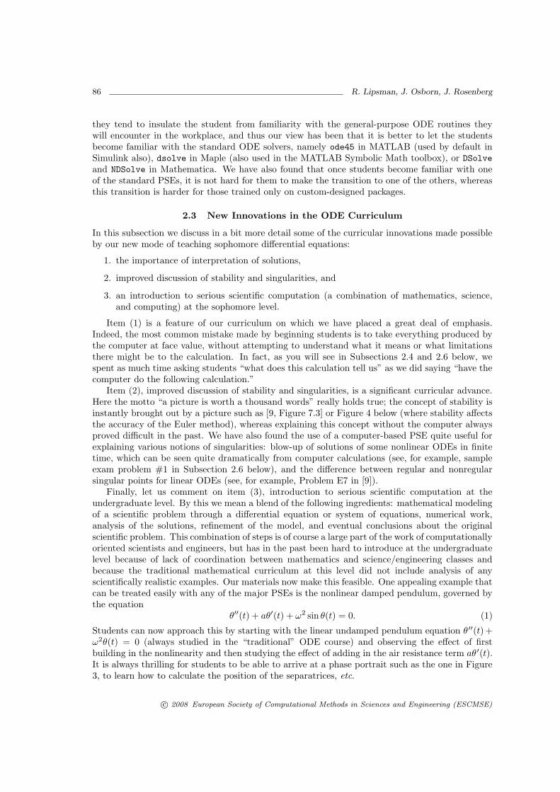
(b) What follows is a short M-file that attempts to solve the above equation numericallyusing MATLAB with different values of the error tolerance, along with the output itgenerated:

t = [0:0.2:0.8, .98];

for j = 1:3

options = odeset(’RelTol’, 3*10^(-j));

sol = ode45(@(t,y) -t/y, [0,1], 1, options);

y = deval(sol, t);

disp(’ t y’), disp([t’, y’])

end

t y

0 1.0000

0.2000 0.9798

0.4000 0.9165

0.6000 0.8000

0.8000 0.6000

0.9800 0.2560

t y

0 1.0000

0.2000 0.9798

0.4000 0.9165

0.6000 0.8000

0.8000 0.6000

0.9800 0.1989

t y

0 1.0000

0.2000 0.9798

0.4000 0.9165

0.6000 0.8000

0.8000 0.6000

0.9800 0.2004

How do you account for the fact that with all three error tolerances, the computed valueof the solution at t = 0, 0.2, 0.4, 0.6 and 0.8 is the same, whereas the computed valuesof the solution at t = 0.98 differ wildly? Which of the three approximate solutions ismost accurate, and why?

2. Suppose the initial value problems

(a)y′ = 2y + e−t, y(0) = −1/3

and

(b)y′ = −2y − e−t, y(0) = 1/3



0 0.2 0.4 0.6 0.8 1 1.2 1.4 1.6 1.8 20

0.2

0.4

0.6

0.8

1

1.2

1.4

1.6

Dy = 2*y−2+3*exp(−x)

x

y

h=0.2h=0.1h=0.05ode45

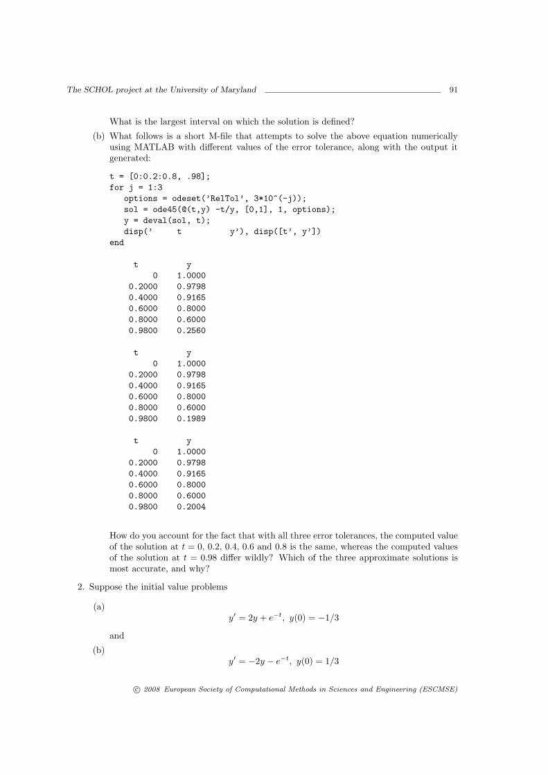
Figure 4: Approximate solution using Euler method with h = 0.2, 0.1, 0.05 and ode45

are solved with ode45 on [0, 10]. For which problem would you have greater confidencein the results? Explain.

3. Consider the initial value problem

dy

dx= 2y − 2 + 3e−x, y(0) = 0.

Figure 4 shows approximations to y(x) obtained with the Euler method with step size h = 0.2(top curve), h = 0.1 (second curve), h = 0.05 (third curve), and with the MATLAB functionode45 (curve with the circles).

(a) Explain the graph in terms of stability of the ODE.

(b) Solve the equation explicitly.

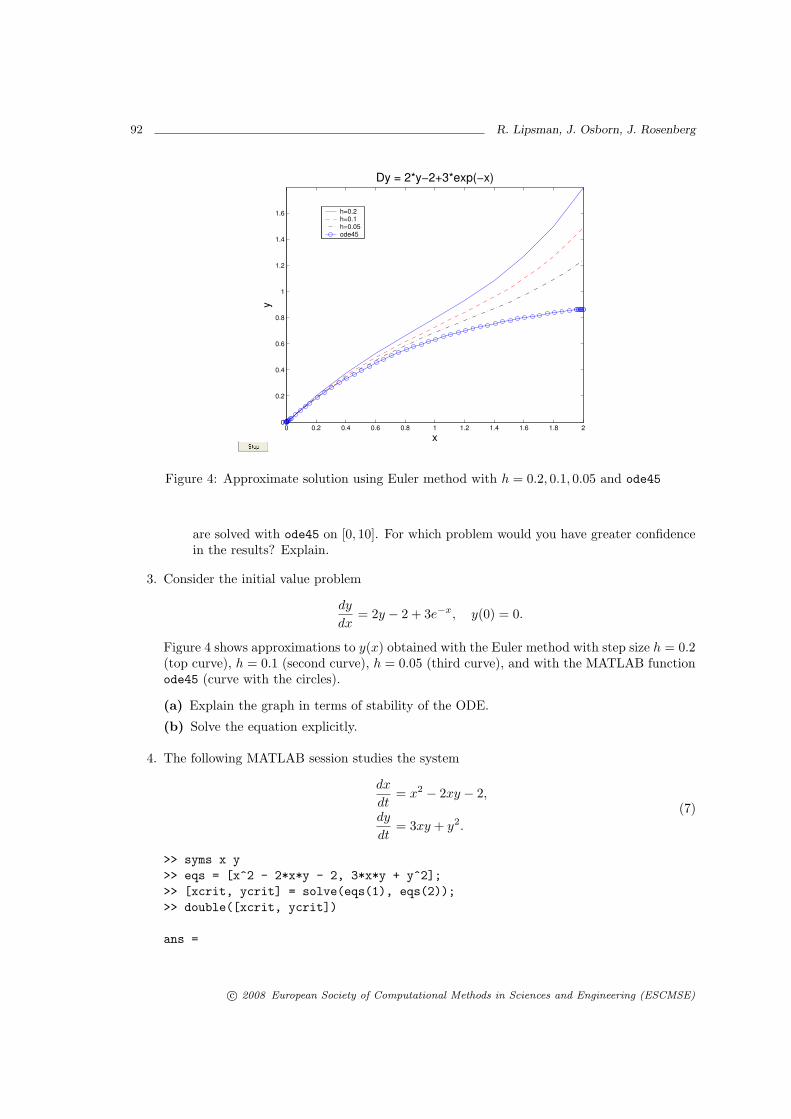
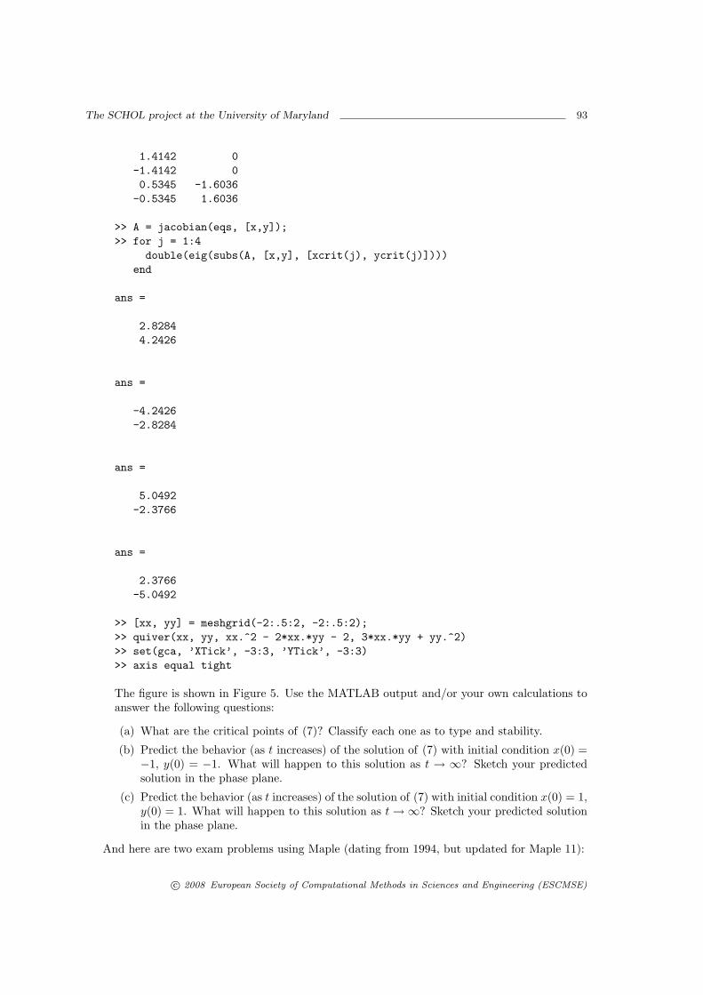
4. The following MATLAB session studies the system

dx

dt= x2 − 2xy − 2,

dy

dt= 3xy + y2.

(7)

>> syms x y

>> eqs = [x^2 - 2*x*y - 2, 3*x*y + y^2];

>> [xcrit, ycrit] = solve(eqs(1), eqs(2));

>> double([xcrit, ycrit])

ans =



1.4142 0

-1.4142 0

0.5345 -1.6036

-0.5345 1.6036

>> A = jacobian(eqs, [x,y]);

>> for j = 1:4

double(eig(subs(A, [x,y], [xcrit(j), ycrit(j)])))

end

ans =

2.8284

4.2426

ans =

-4.2426

-2.8284

ans =

5.0492

-2.3766

ans =

2.3766

-5.0492

>> [xx, yy] = meshgrid(-2:.5:2, -2:.5:2);

>> quiver(xx, yy, xx.^2 - 2*xx.*yy - 2, 3*xx.*yy + yy.^2)

>> set(gca, ’XTick’, -3:3, ’YTick’, -3:3)

>> axis equal tight

The figure is shown in Figure 5. Use the MATLAB output and/or your own calculations toanswer the following questions:

(a) What are the critical points of (7)? Classify each one as to type and stability.

(b) Predict the behavior (as t increases) of the solution of (7) with initial condition x(0) =−1, y(0) = −1. What will happen to this solution as t → ∞? Sketch your predictedsolution in the phase plane.

(c) Predict the behavior (as t increases) of the solution of (7) with initial condition x(0) = 1,y(0) = 1. What will happen to this solution as t→∞? Sketch your predicted solutionin the phase plane.

And here are two exam problems using Maple (dating from 1994, but updated for Maple 11):



−2 −1 0 1 2

−2

−1

0

1

2

Figure 5: Output from the MATLAB session

5. The Maple figure in Figure 6 depicts the direction field of a first order autonomous differentialequation y′ = f(y).

(a) Indicate the equilibrium solutions of the differential equation and discuss their stability.

(b) Which of the following expressions could be f(y)? More explicitly, explain why eachcandidate could or could not serve as f(y).

i. y(y − 1)(y − 2)

ii. y2(y − 1)(y − 2)

iii. −y2(y − 2)2

��

��

�

�

�

�

Figure 6: A direction field plotted in Maple



6. State the Sturm Comparison Theorem. (Hint: It concerns two differential equations y ′′ +q(x)y = 0 and y′′ + r(x)y = 0 on an interval [a, b].) Now examine the following MapleWorksheet and answer these questions:

(a) What is the interval [a, b] under consideration?

(b) Identify the functions q(x) and r(x).

(c) What conclusion of the comparison theorem is verified in the graph?

sol1 := dsolve({diff(y(x), x, x) + π2 · y(x) = 0, y(0) = 0, D(y)(0) = π}, y(x));

y (x) = sin (π x)

plot({π2, 2 · π2 · (1− exp(−x))}, x = 0..2);

��

�

�

�

�

� �

� �

� �

� �

sol := dsolve({diff(y(x), x, x) + 2 · π2 · (1− exp(−x)) · y(x) = 0,y(0) = 1, D(y)(0) = 0}, y(x), numeric,maxfun = 1000);

proc (x rkf45 ) ... endproc

with(plots) :biggersol := odeplot(sol, [x, y(x)], 1..2) :smallersol := plot(rhs(sol1), x = 1..2, style = POINT, symbol = BOX) :display({biggersol, smallersol});



�� !

"

# �� !

# !��

# !��

# !��

# !��

!�� !

!��

!��

!��

2.7 Comparison of PSEs

Since we have developed materials for all the major PSEs (MATLAB, Mathematica, and Maple),we should say something about their relative advantages and disadvantages from the point ofview of teaching sophomore ODE. First of all, as we said before, we have found the differencesbetween these various packages to be relatively minor, compared to the features that they allshare in common. Secondly, we have found that the differences have tended to dissipate withtime. In the early 90s, Mathematica and Maple emphasized their “front ends,” called notebooksand worksheets, respectively, whereas MATLAB more closely resembled conventional programminglanguages such as FORTRAN. That tended to make numerical calculation faster in MATLAB, butMathematica and Maple were more convenient for producing finished documents in a single step(without having to run code, save the output, and paste it into a document). Back in the 90s,MATLAB was superior for numerical calculation, especially for calculations involving matrices.While MATLAB is still superior for numerical linear algebra, nowadays these differences no longermatter much in a beginning ODE course. While efficiency and speed are still relevant issues forlarge-scale computations, as desktop and laptop computers have become faster, speed is no longermuch of a consideration in the relatively small calculations likely to arise in a sophomore course.On the other hand, the “front ends” of all of the major PSEs have been improved to the pointwhere they all can be used to produce finished documents incorporating descriptive text, code,numerical or symbolic output, and graphics. And finally, when we started the SCHOL project inthe 90s, there were significant differences between the sorts of problems that could be handled byeach of the major PSEs. (For example, some did not work very well with solutions going backwardsand forwards in time, etc. And there were various strange bugs, which have mostly been fixed sincethen, in many of the symbolic ODE solvers, often having to do with choosing the wrong branch ofmultivalued transcendental functions.) Most of these differences have since disappeared, so thatthe instructor who wants to use our materials in sophomore ODE can now choose among thePSEs on the basis of non-curricular issues (local campus support, price, licensing agreements, etc.)without there being much effect on quality of the curriculum.



3 Non-Curricular Issues

In this section we will describe the non-curricular issues that arose over the years in our projectto incorporate technology into the sophomore level ordinary differential equations course. Therewere many such issues. They included:

• support, or lack thereof, of the department administration.

• support and cooperation, or lack thereof, of our fellow faculty.

• receptivity of the students to the introduction into the course of what they perceived, at leastinitially, as new material, in addition to the normal course material.

• the choice of requiring computers in the classroom (e.g., mandate laptops or conduct classesonly in computer labs), or expecting that the students’ computer work would take placeoutside of class.

• the charge that our new version of the course would require additional time to be devoted tothe course—both by students and faculty; and if true, how can it be justified?

• the choice of class format that would work best with our version of the course—small classes,large lectures, computer teaching labs, or some other.

• frequent pressure from publishers to update our materials, especially as new versions of thesoftware emerge.

• additional student costs, e.g., to buy student copies of the software, or to purchase softwareprimers or course supplements.

• pressure from clients around campus (primarily Engineering) to emphasize certain softwarepackages at the expense of others.

• the choice of format in which to publish our material: university class notes, supplement toODE text (specific or generic), or a full fledged book.

In what follows we discuss each of these issues, describe how we dealt with them, and assesswhat success we had in those dealings.

3.1 Support of Departmental Administrators

One of the first critical issues we faced was the support of our departmental administrators, i.e.,the Chair, Director of Undergraduate Studies, and the Undergraduate Curriculum Committee.What we were proposing would involve a major change to one of the most stable courses in theMathematics Department, one whose curriculum and method of delivery had remained unchangedfor many years. And since we anticipated some resistance on the part of our colleagues and students,we knew that obtaining the prior enthusiastic support of the department’s leaders in education wascrucial. We were at best only partially successful. The ambivalence that we anticipated amongour colleagues was reflected in departmental discussions of our proposal. Furthermore, perhapsgauging the political winds, the Chair was supportive, but his support was best described as tepid.

In the end, after painstaking and time-consuming lobbying on our part, the Chair and all theappropriate departmental committees gave their “qualified” blessing for our project to proceed.However, they did not commit any additional resources to the teaching of the course. There is noquestion that the lack of unreserved support for our efforts had some deleterious effects. For ex-ample, negative whispers in the halls caused some faculty who might have participated to hesitate.



Others who did participate, did so with some trepidation. We had to do our own advertising andpromotion in the Engineering College—without the overt backing of the departmental administra-tion. Students, also sensing some reluctance on the part of the department, felt free to complainin ways they might not have had they sensed wholesale support. None of these problems was fatal,and the fact that, 16 years after its inception, our vision for the content and delivery of sophomoreODE has been implemented and is the “law of the land,” proves that our project was deployedsuccessfully. But we believe unquestionably that had we had the enthusiastic and unqualified sup-port of the department from the beginning, including additional resources, our project would havebeen deployed more quickly, with wider participation and greater impact than it enjoyed.

3.2 Faculty Support

The issue of faculty support was also crucial for the success of our project. We spent many hoursexplaining our motivations and goals to our colleagues. Quite a few understood and sympathizedwith our objectives, and these taught the course enthusiastically using our materials as they weredeveloped. But a not insubstantial number were less enthusiastic. They worried about severalthings: the extra time they thought would be required of them; the possible need to eliminatetopics from the established syllabus in order to accommodate the software; their ability to masterthe software sufficiently so that they could meaningfully respond to student requests for assistance;reliance on hardware and software that might prove unreliable (recall this was happening duringa period when the concept of computer-aided course work was still in its infancy); inexperience indesigning test materials suitable for a mathematical software environment. All of these concernsinfluenced us as we continued to develop and redevelop our material throughout the 1990s.

In the end we believe that we met these concerns forthrightly and successfully. The facultyappreciated our responsiveness and eventually the use of mathematical software was made manda-tory in the sophomore ODE course. The number of faculty—both regular and visiting—who havetaught successfully at Maryland using our materials is truly astounding. Other faculty (and someof us) developed software materials for other sophomore courses (linear algebra and multi-variablecalculus). Today it is accepted practice by all who teach sophomore math courses at College Parkthat software is an integral part of the curriculum. So one of our primary goals (creating thesophomore software gateway) was achieved. This gives us much satisfaction. But there is oneunfortunate practice that survives from the days of the early skeptics. It manifests itself in per-haps 10-15% of the faculty who teach the course. Namely, they resent the intrusion of what theysee as at best a tool into the heart of the course and they deal with it according to a methoddescribed best in a phrase coined by one of us: they sniff around the edges. They do not familiarizethemselves with the software more than in a casual sense; they deemphasize it in class; they sendsoftware questions to the TAs; they continue to emphasize classical symbolic solution techniquesover numerical and qualitative methods; in short, they try to recreate the classroom environmentthat obtained in 1975. By doing so they shortchange their students, and they shortchange them-selves. We are grateful that the number of such lecturers is small, but there is no question thatthey have had a negative influence on faculty support. This phenomenon might diminish as moreyoung faculty come on board.

3.3 Student Cooperation

We wondered how our students would react to this major change in a traditional course. The vastmajority were engineering majors—far more than the math or physics majors who took the course.Would they realize that by exposing them to a mathematical software tool and a heightened numer-ical and graphical environment, we were enhancing their preparation for the professional challengesthat awaited them; or would they merely see the change as a needless complication of their program



of study? Well, aside from the not surprising bumps and potholes (i.e., locked computer labs, in-compatible printers, occasionally confused instructors), we were pleasantly surprised by the speedand equanimity with which our students acclimated themselves to the new mode. Moreover, astime went by, the percentage of our students who were exposed to a mathematical software systembefore they entered our course grew markedly. And those who were not so exposed a priori werealso not disgruntled about encountering it; indeed the time it took for our (unexposed) students to“get up to speed” shrunk from year to year. Students never complained that they had to learn lessabout series solutions because they and their instructors had to spend time on the software. Theydid complain about the glitches—sometimes vociferously. But as we explained earlier, we believetheir complaints might have been less forceful had they not been exposed to the small number ofrecalcitrant faculty. In any event, once the gateway was opened, it is fair to say that the studentsmarched through it with scarcely a stumble.

3.4 The Computer Environment

From the inception of our project we had a very clear idea of how we wanted the introduction ofa mathematical software system to influence the curriculum of the sophomore ODE course. Whatwas less clear to us was the precise format by which the students would access the software. Weentertained many ideas:

• require that each student come to class equipped with a laptop on which the software wasloaded;

• present the course in a computer lab in which students would access the software on auniversity-owned desktop;

• use the preceding scheme, but in a more elaborate venue. The University of Maryland wasone of the national pioneers of teaching theaters—basically computer labs in which all thestudent desktops and the faculty desktop are closely networked. The University had twosuch theaters in the early 1990s;

• don’t require students to have computer access in class, but insist that the faculty memberhave the software available on the lecturer’s desktop with the ability to project its screen tothe students;

• ask the faculty lecturer only occasionally to bring a computer to class for demonstrationsand presentations;

• operate with no computers in class, but ensure that students have access to the softwarethrough student versions for their own computers and, more commonly, well-equipped com-puter labs around campus.

To be honest we had differing opinions about which mode was most desirable. But in the end,cost and logistics made the decision for us. Keep in mind that this decision process was taking placein the early 1990s. To require that all of our students (at a large state university, many of whoseenrollees had financial challenges) should acquire laptops was far beyond the realm of possibility.The theater option was appealing and we experimented with it, but there were not nearly enoughseats to accommodate the hundreds of students who took the course each semester. There weremore regular computer lab seats, but still not nearly enough. There were also an insufficientnumber of classrooms with computer access for the instructor; nor was the university inclined (atthat time) to invest the resources to correct that situation. Also, for reasons already discussed, nottoo many faculty were clamoring for such a development. Some of us did do computer demos andpresentations in class, but it really didn’t take us long to realize that the last described mode (the



computer-less classroom) was the default solution. In the end, that relatively low tech solutiondovetailed rather nicely with a key feature of the course as it evolved. Namely, we replaced manyrote formula solution problems by mini computer-aided projects, as we have already discussed.The students worked on these projects alone or in groups, in their dorms or in computer labs, andthus the format selected worked well to implement our vision. Our students took to this formatrather well and many did excellent work. On the other hand, that work resulted in lots of gradingfor us—a nice segue to the next topic.

3.5 Additional Time

From the outset we believed that the charge of “extra time” was a red herring. We saw—andcontinue to see—that the responsibility of our department is to provide our students with the mostmodern, relevant and useful education in mathematics—one that they could use successfully inacademia, a federal research lab, or in the business world. If a topic in physics or chemistry evolvesto the point that the lab component of an allied course must be radically altered or augmented,no one questions the suitability of revising the curriculum. If extra time is mandated, the facultycarefully examine the curriculum and decide what current material, if any, must be replaced. If thenature of the change might necessitate increased time in the lab by faculty and/or students, that isviewed as the price of modernization. Well, exactly the same principles apply to mathematics. Anintegrated curriculum incorporating symbolic, graphical, numeric and computational techniquesis the right way to teach 21st century ODE—even to sophomores. If we don’t implement such acurriculum, we are shirking our responsibility. If additional time or effort is required of facultyand/or students, it is unavoidable—and by the way, likely only temporary. Our impression is thatthis self-evident assertion was recognized more quickly by the students than by the faculty, buteventually everyone got it.

3.6 Class Format

At the beginning of the project, especially when we were uncertain of the means of student com-puter access, we also pondered the best format in which to deliver our course. Traditionally, thecourse had been taught in (relatively) small classes (25-35 students) by a professorial faculty mem-ber. Occasionally a visitor or an exceptionally qualified lecturer might be assigned a section, butgenerally the task fell to regular faculty. Because of the huge number of engineering students, therewere semesters in which the number of sections reached ten or more. Naturally—for the reasonsalready alluded to—we worried about securing the services of a reasonable number of faculty who,if not completely dedicated to our vision, would at least be sufficiently qualified and enthusiasticto deliver the course in the manner we intended. So we considered the classic large lecture formator more moderately-sized large lectures in computer labs. This would cut the number of facultynecessary, but of course introduce the problem of qualified TAs. Could we find enough of them?4

But as with the issue of access, the class format decision was made for us by the available facili-ties. At that time there were insufficient lecture hall facilities to move to a large lecture format.Thus, we produced some help materials for faculty; we did a lot of hand-holding; and we madeourselves widely available to our colleagues for their questions. With these compromises and a lotof encouragement, we were able to develop a large cadre of faculty lecturers who could and diddeliver the course in small classes. This is highly ironic, because in the budget crunch of the early2000s, the Math Department converted the course to a large lecture format, which required veryfew faculty (but a large number of TAs) to run the course effectively. But we are pleased to saythat it is still running very smoothly. So in the end, we concluded that our version of sophomoreODE should succeed in virtually any class format.

4To be truthful, we were less concerned about finding qualified TAs than we were about finding qualified faculty.



3.7 Publisher Pressure

We were fortunate at the beginning of our work to find a publisher with a successful ODE textbookwho saw the potential to modernize and enhance the value of their book by adopting our visionfor the ODE course. They encouraged the author to welcome a supplement that they believedwould boost the appeal of their product. The publisher was John Wiley and Sons, Inc., the authorwas William Boyce, and the book was Elementary Differential Equations (the latest edition is[2]). However, from the outset, they wanted us to write editions of our supplement in all threePSEs—Mathematica, Maple and MATLAB, and to keep our books current with the latest versionof each software package. Thus ensued a constant tension between us. As important as it is thatbooks keep up with changes in software, because of other constraints on our schedules, we found thepublisher’s demands difficult to meet. Although there were many common features of Mathematica,Maple and MATLAB, there were also significant differences. It’s a little like Romance languages.Being fluent in French (Mathematica) guarantees only that one is at best minimally conversantin Italian (Maple). Moreover the software companies produce new versions too frequently. Infact we have produced two editions of our materials for each of the three PSEs ([3], [4], [5], [6],and [8], [9]), and a new edition of the Maple version will be out soon [7]. We appreciate thepublisher’s motivation, but we have found this pressure a burden; although to be honest softwareimprovements in recent versions of all three products—especially in their interfaces—have greatlyabetted the implementation of our vision for sophomore ODE.

3.8 Student Costs

Naturally, the concern of additional costs to the students was raised as we developed our newmaterials. These costs might include:

• the cost of our “book,” which would be in addition to the cost of the primary text;

• the cost of a primer or any other help material students might need to get started usingthe software—which, at least at the outset of our project, it was unlikely that they hadencountered previously;

• the cost of purchasing a student version if we made their ownership of the software mandatory;

• possible tutorial costs if they needed additional help in acclimating to the software environ-ment.

We were very sensitive to these concerns. The costs of books and educational materials thatstudents cope with were (and continue to be) very burdensome. We did not want to add to theirfinancial woes. And so in planning and deployment we addressed each of the four issues above.We wrote a paperback supplement rather than a full blown textbook—more on that choice later.We incorporated enough material on the software in the supplement to enable students to getup to speed without the need for an additional primer. We arranged for a campus software sitelicense and widespread availability of the software in departmental and campus computer labs. Weconvinced the Math Department to partner with the campus computer services organization toplan and offer free software tutorials. Finally, the switch to a single software package (MATLAB),which students were already using in their engineering courses, effected a cost savings for students.All of these efforts proved quite successful and we heard little or no complaining about additionalcosts from our students.



3.9 Campus Clients

Like all Math Departments in large state universities, ours in College Park carries an enormousservice load. We have lower level (and some upper level) courses designed to serve the needs of stu-dents in business, social sciences, education, physical and life sciences, and especially engineering.We take pride in the care and attentiveness with which we design and deliver these courses. Nowwe already mentioned that our seminal effort began in Mathematica and that we added Maple afew years later. The rub was that the engineers were already incorporating MATLAB into theircourses and they were not particularly pleased that we were offering ODE using Mathematica andMaple but not MATLAB. So we introduced MATLAB. But that only made matters worse as theEngineering students clamored to get into MATLAB sections and felt discriminated against whenlimited seats drove them into sections offering one of the other software systems. Engineeringcontinued to apply pressure and eventually we relented—all of our ODE sections now use MAT-LAB. We surrendered in part because of our desire to treat our clients well and in part because webecame convinced that all three softwares—despite differing strengths and weaknesses—were morethan adequate for our purposes, and so we saw no political or academic advantage to resisting theengineers.

3.10 Project Format

We already explained an important reason for our choice to publish our work in the form of asupplement to Boyce’s ODE book. Namely, it played a key role in keeping down student costs.But we had other reasons for producing a supplement as opposed to say a full blown textbook onone hand or a simple set of classroom notes on the other. The reason not to do the latter wassimple and obvious. We believed that our ideas were relevant to the delivery of sophomore ODE allover the country and we wanted to market our ideas in a format that would reach a wider audience.So why not a textbook? Student costs were germane but not the primary driving factor. All ofthe participants had active research programs. None of us had the desire to compete in the majortextbook market. We would not have objected to better royalties, but we were most reluctant toenter the world of constant revisions, short publisher deadlines, and loss of control over academiccontent that we had observed among local and national colleagues who had traveled that route.

In retrospect, we question the wisdom of that decision. It took us a long time to realize that ourpublisher’s primary goal in their (very limited) promotion of our supplement was almost exclusivelyto boost the sales of Boyce’s book. The number of adoptions of our book and the exposure of ourideas would have been much greater if we had published a textbook instead of a supplement. Ahwell, water under the bridge.

Collaborators

Those who have checked the Bibliography will have noticed that there are current editions of theMaple and MATLAB versions of our book, but not the Mathematica version. The new Mapleversion [7] was accomplished through a collaboration with Larry Lardy of Syracuse University.Plans are now in place to prepare a new Mathematica version through a collaboration with DonaldOuting of the United States Military Academy. We really appreciate the expertise and enthusiasmthat Professors Lardy and Outing have added to the SCHOL project.

Acknowledgments

The project we described here was the work of a large number of people over a long period of time.We want to thank especially the other members of the SCHOL project: Kevin Coombes, Brian



Hunt, and Garrett Stuck for their contributions. We received support and encouragement frommany other colleagues in the Mathematics Department and the Office of Information Technologyat the University of Maryland, and from colleagues around the country who have given us feedbackand comments on our materials.

During the preparation of this paper, John Osborn was partially supported by NSF grant DMS-0611094. Jonathan Rosenberg was partially supported by NSF grant DMS-0504212. Any opinions,findings, and conclusions or recommendations expressed in this material are those of the authorsand do not necessarily reflect the views of the National Science Foundation.

References

[1] P. Blanchard, R. L. Devaney and G. R. Hall, Differential Equations, 3rd ed., Brooks/Cole,2005.

[2] W. E. Boyce and R. C. DiPrima, Elementary Differential Equations, 8th ed., Wiley, 2004.

[3] K. R. Coombes, B. R. Hunt, R. L. Lipsman, J. E. Osborn, and G. J. Stuck, DifferentialEquations with Mathematica, Wiley, 1995.

[4] K. R. Coombes, B. R. Hunt, R. L. Lipsman, J. E. Osborn, and G. J. Stuck, DifferentialEquations with Mathematica, 2nd ed., Wiley, 1998.

[5] K. R. Coombes, B. R. Hunt, R. L. Lipsman, J. E. Osborn, and G. J. Stuck, DifferentialEquations with Maple, Wiley, 1996.

[6] K. R. Coombes, B. R. Hunt, R. L. Lipsman, J. E. Osborn, and G. J. Stuck, DifferentialEquations with Maple, 2nd ed., Wiley, 1997.

[7] B. R. Hunt, L. J. Lardy, R. L. Lipsman, J. E. Osborn, and J. M. Rosenberg, DifferentialEquations with Maple, 3rd ed., Wiley, 2008, to appear.

[8] K. R. Coombes, B. R. Hunt, R. L. Lipsman, J. E. Osborn, and G. J. Stuck, DifferentialEquations with MATLAB, Wiley, 2000.

[9] B. R. Hunt, R. L. Lipsman, J. E. Osborn, and J. M. Rosenberg, Differential Equations withMATLAB, 2nd ed., Wiley, 2005.

[10] J. C. Polking and D. Arnold, Ordinary Differential Equations Using MATLAB, 3rd ed., Pren-tice Hall, 2004.

[11] D. Schwalbe and S. Wagon, VisualDSolve: Visualizing Differential Equations with Mathe-matica, TELOS, Springer, 1997.

[12] K. R. Coombes, R. L. Lipsman, and J. M. Rosenberg, Multivariable Calculus and Mathematica,TELOS, Springer, 1998.

[13] B. R. Hunt, R. L. Lipsman, and J. M. Rosenberg, A Guide to MATLAB, Cambridge Univ.Press, 2001.

[14] B. R. Hunt, R. L. Lipsman, and J. M. Rosenberg, A Guide to MATLAB, 2nd ed., CambridgeUniv. Press, 2006.

[15] K. R. Coombes, B. R. Hunt, R. L. Lipsman, J. E. Osborn, and G. J. Stuck, The MathematicaPrimer, Cambridge Univ. Press, 1998.


the schol project at the university of maryland: …€¦ · ronald l. lipsman, ... enrich the...

Documents