The Role of the Structural Transformation

in Aggregate Productivity†

Margarida Duarte

University of Toronto

Diego Restuccia

University of Toronto

February 2009

Abstract

We investigate the role of sectoral differences in labor productivity in explaining the processof structural transformation – the secular reallocation of labor across sectors – and the timepath of aggregate productivity across countries. Using a simple model of the structuraltransformation that is calibrated to the growth experience of the United States, we measuresectoral labor productivity differences across countries. Productivity differences betweenrich and poor countries are large in agriculture and services and smaller in manufacturing.Moreover, over time, productivity gaps have been substantially reduced in agriculture andindustry but not nearly as much in services. In the model, these sectoral productivitypatterns generate implications that are broadly consistent with the cross-country evidenceon the structural transformation, aggregate productivity paths, and relative prices. We showthat productivity catch-up in industry explains about 50 percent of the gains in aggregateproductivity across countries, while low relative productivity in services and the lack ofcatch-up explains all the experiences of slowdown, stagnation, and decline observed acrosscountries.

Keywords: labor productivity, structural transformation, sectoral productivity, employment,hours, cross-country data.JEL Classification: O1,O4.

†We thank the editor and three referees for very useful and detailed comments. We also thank commentsand suggestions from Tasso Adamopoulos, John Coleman, Mike Dotsey, Gary Hansen, Gueorgui Kambourov,Richard Rogerson, Marcelo Veracierto, Xiaodong Zhu, and audiences at ASU Economic Development Work-shop, Inter-American Development Bank, Society for Economic Dynamics Meetings, University of Sydney,Winter Meetings of the Econometric Society, Wharton School, University of Pennsylvania, ITAM SummerCamp, Queen’s University, and University of Rochester. Andrea Waddle provided excellent research as-sistance. All errors are our own. We gratefully acknowledge the support from the Connaught Fund atthe University of Toronto (Duarte) and the Social Sciences and Humanities Research Council of Canada(Restuccia). Contact Information: Department of Economics, University of Toronto, 150 St. George Street,Toronto, ON M5S 3G7, Canada. E-mail: margarida.duarte@utoronto.ca; and diego.restuccia@utoronto.ca.

1

1 Introduction

It is a well-known observation that over the last 50 years countries have experienced remark-

ably different paths of economic performance.1 Looking at the behavior of GDP per hour

of individual countries relative to that of the United States we find experiences of sustained

catch-up, catch-up followed by a slowdown, stagnation, and even decline (see Figure 1 for

some illustrative examples).2 Consider for instance the experience of Ireland. Between 1960

and 2004, GDP per hour in Ireland relative to that of the United States rose from about 35

percent to about 75 percent.3 Spain also experienced a period of rapid catch-up to the United

States from 1960 to around 1990, a period during which relative GDP per hour rose from

about 35 to 80 percent. Around 1990, however, this process slowed-down dramatically and

relative GDP per hour in Spain stagnated and later declined. Another remarkable growth

experience is that of New Zealand where GDP per hour fell from about 70 to 60 percent of

that of the United States between 1970 and 2004.

Along their modern path of development countries undergo a process of structural trans-

formation by which labor is reallocated among agriculture, industry, and services. Over

the last 50 years many countries have experienced substantial amounts of labor reallocation

across sectors. For instance, from 1960 to 2004, the share of hours in agriculture in Spain

fell from 44 to 6 percent while the share of hours in services rose from 25 to 64 percent. In

about the same period, the share of hours in agriculture in Belgium fell just from 7 to 2

percent, while the share in services rose from 43 to 72 percent.

In this paper we study the behavior of GDP per hour over time from the perspective

of sectoral productivity and the structural transformation.4 Does a sectoral analysis con-

tribute to the understanding of aggregate productivity paths? At a qualitative level, the

answer to this question is clearly yes. Since aggregate labor productivity is the sum of labor

1See Chari, Kehoe, and McGrattan (1996), Jones (1997), Prescott (2002), Duarte and Restuccia (2006),among many others.

2We use GDP per hour as our measure of economic performance. Throughout the paper we refer to laborproductivity, output per hour, and GDP per hour interchangeably.

3All numbers reported refer to trended data using the Hodrick-Prescott filter. See Section 2 for details.4See Baumol (1967) for a discussion of the implications of structural change on aggregate productivity

growth.

2

productivity across sectors weighted by the share of labor in each sector, the structural trans-

formation matters for aggregate productivity. At a quantitative level the answer depends on

whether there are substantial differences in sectoral labor productivity across countries. Our

approach in this paper is to first develop a simple model of the structural transformation

that is calibrated to the growth experience of the United States. We then use the model to

measure sectoral labor productivity differences across countries at a point in time. These

measures, together with data on sectoral labor productivity growth, imply time paths of

sectoral labor productivity across countries. We use these measures of sectoral productivity

in the model to assess their quantitative role on the structural transformation and aggregate

productivity outcomes across countries.

We find that there are large and systematic differences in sectoral labor productivity

across countries. In particular, differences in labor productivity levels between rich and

poor countries are larger in agriculture and services than in manufacturing. Moreover, over

time, productivity gaps have been substantially reduced in agriculture and industry but

not nearly as much in services. To illustrate the implications of these sectoral differences

for aggregate productivity, imagine that these productivity differences remain constant as

countries undergo the structural transformation. Then as developing countries reallocate

labor from agriculture to manufacturing, aggregate productivity can catch-up as labor is

reallocated from a low relative productivity sector to a high relative productivity sector.

Instead, countries further along the structural transformation can slowdown, stagnate, and

decline as labor is reallocated from industry (a high relative productivity sector) to services

(a low relative productivity sector). When the time series of sectoral productivity are fed

into the model of the structural transformation, we find that high labor productivity growth

in industry relative to that of the United States explains about 50 percent of the catch-up in

relative aggregate productivity across countries. Although there is substantial catch-up in

agricultural productivity, we show that this factor contributes little to aggregate productivity

gains. In addition, we show that low relative productivity in services and the lack of catch-

up explains all the experiences of slowdown, stagnation, and decline in relative aggregate

productivity observed across countries.

3

We construct a panel data set on PPP-adjusted real output per hour and disaggregated

output and hours worked for agriculture, industry, and services. Our panel data includes

29 countries with data covering the period from 1956 to 2004 for most countries.5 From

these data, we document three basic facts. First, countries follow a common process of

structural transformation characterized by a declining share of hours in agriculture over

time, an increasing share of hours in services, and a hump-shaped share of hours in industry.

Second, there is substantial lag in the process of structural transformation for some countries

and this lag is associated with the level of relative income. Third, there are sizable and

systematic differences in sectoral growth rates of labor productivity across countries. In

particular, most countries observe higher growth rates of labor productivity in agriculture

and manufacturing compared to services. In addition, countries with high growth rates of

aggregate productivity tend to have much higher productivity growth in agriculture and

manufacturing than the United States, but this strong relative performance is not observed

in services. Countries with low growth rates of aggregate labor productivity tend to observe

low labor productivity growth in all sectors.

We develop a simple general equilibrium model of the structural transformation with three

sectors − agriculture, industry, and services. Following Rogerson (2008), labor reallocation

across sectors is driven by two channels: income effects due to non-homothetic preferences

and substitution effects due to differential productivity growth across sectors.6 We calibrate

the model to the structural transformation of the United States between 1956 and 2004.

A model of the structural transformation is essential for the purpose of this paper for two

reasons. First, we use the calibrated model to measure sectoral productivity differences

across countries at one point in time. This step is needed because of the lack of comparable

(PPP-adjusted) sectoral output data across a large set of countries. Second, the process of

structural transformation is endogenous to the level and changes over time in sectoral labor

productivity. As a result, a quantitative assessment of the aggregate implications of sectoral

5Our sample does not include the poorest countries in the world: the labor productivity ratio betweenthe richest and poorest countries in our data is only 10.

6For recent models of the structural transformation emphasizing non-homothetic preferences seeKongsamut, Rebelo, and Xie (2001) and emphasizing substitution effects see Ngai and Pissarides (2007).

4

productivity differences requires that changes in the distribution of labor across sectors be

consistent with sectoral productivity paths.

The model implies that sectoral productivity levels in the first year in the sample tend

to be lower in poor than in rich countries, particularly so in agriculture and services. In-

terestingly, the model implies low dispersion in productivity levels in manufacturing across

countries. We argue that these differences in sectoral labor productivity implied by the

model are consistent with the available evidence from studies using producer and micro data

for specific sectors, for instance Baily and Solow (2001) for manufacturing and service sectors

and Restuccia, Yang, and Zhu (2008) for agriculture. The levels of productivity implied by

the model together with data on sectoral labor productivity growth for each country, imply

time paths for sectoral productivity in each country. Given these time paths for productivity,

the model reproduces the broad patterns of labor reallocation and aggregate productivity

growth across countries. The model also has implications for sectoral output and relative

prices that are broadly consistent with the cross-country data.

This paper is related to a large literature studying income differences across countries.

Closely connected is the literature studying international income differences in the context

of models with delay in the start of modern growth.7 Since countries in our data set have

started the process of structural transformation well before the first year in the sample pe-

riod, our focus is on measuring sectoral productivity across countries at a point in time

and on assessing the role of their movement over time in accounting for the patterns of

structural transformation and aggregate productivity growth across countries.8 Our paper is

also closely related to a literature that emphasizes the sectoral composition of the economy

in aggregate outcomes, for instance Restuccia, Yang, and Zhu (2008), Cordoba and Ripoll

(2004), Vollrath (2009), Chanda and Dalgaard (2005), Coleman (2007), and Adamopoulos

and Akyol (2007).9 In studying labor productivity over time, our paper is related to a litera-

7See, for instance, Lucas (2000), Hansen and Prescott (2002), Ngai (2004), and Gollin, Parente, andRogerson (2002).

8Herrendorf and Valentinyi (2006) also consider a model to measure sectoral productivity differencesacross countries but instead use expenditure data from the Penn World Table.

9See also Caselli and Tenreyro (2006) and the survey article by Caselli (2005).

5

ture studying country episodes of slowdown and depression.10 Most of this literature focuses

on the role of exogenous movements in aggregate total factor productivity and aggregate

distortions on GDP relative to trend. We differ from this literature by emphasizing the

importance of sectoral labor productivity on the structural transformation and the secular

movements in relative GDP per hour across countries.

The paper is organized as follows. In the next section we document some facts about the

process of structural transformation and sectoral labor productivity growth across countries.

Section 3 describes the economic environment and calibrates a benchmark economy to U.S.

data for the period between 1956 to 2004. In section 4 we discuss our quantitative experiment

and perform counterfactual analysis. We conclude in section 5.

2 Some Facts

In this section, we document the process of structural transformation and labor productivity

growth in agriculture, industry, and services for the countries in our data set at an annual

frequency. Since we focus on long-run trends, data are trended using the Hodrick-Prescott

filter with a smoothing parameter λ = 100. The appendix provides a detailed description of

the data.

2.1 The Process of Structural Transformation

The reallocation of labor across sectors over time is typically referred to in the economic

development literature as the process of structural transformation. This process has been

extensively documented.11 The structural transformation is characterized by a systematic

fall in the share of labor allocated to agriculture over time, by a steady increase in the share

of labor in services, and by a hump-shaped pattern for the share of labor in manufacturing.

That is, the typical process of sectoral reallocation involves an increase in the share of labor

in manufacturing in the early stages of the reallocation process, followed by a decrease in

10See Kehoe and Prescott (2002) and the references therein.11See, for instance, Kuznets (1966), Maddison (1980), among others.

6

the later stages.12

We document the processes of structural transformation in our data set by focusing on

the distribution of labor hours across sectors. We note, however, that this characterization is

very similar to the one obtained by looking at shares of employment. Our panel data covers

countries at very different stages in the process of structural transformation. For instance,

our data includes countries that in 1960 allocated about 70 percent of their labor hours to

agriculture (e.g., Turkey and Bolivia), as well as countries that in the same year have shares

of hours in agriculture below 10 percent (e.g., the United Kingdom). Despite this diversity

in the stage of structural transformation across the sample, all countries follow a common

process of structural transformation. First, all countries exhibit declining shares of hours in

agriculture, even the most advanced countries in this process, such as the United Kingdom

and the United States. Second, countries at an early stage of the process of structural trans-

formation exhibit a hump-shaped share of hours in industry, while this share is decreasing

for countries at a more advanced stage. Finally, all countries exhibit an increasing share

of hours in services. To illustrate these features, Figure 2 plots sectoral shares of hours for

Greece, Ireland, Spain, and Canada.

The processes of structural transformation observed in our sample suggest two additional

observations. First, the lag in the structural transformation observed across countries is

systematically related to the level of development: poor countries are the ones with the

highest shares of hours in agriculture, while rich countries are the ones with the lowest

shares. (See for instance Gollin, Parente, and Rogerson (2007) and Restuccia, Yang, and

Zhu (2008) for a detailed documentation of this fact for shares of employment across a wider

range of countries.) Second, our data suggest the basic tendency for countries that start the

process of structural transformation later to accomplish a given amount of labor reallocation

faster than those countries that initiated this process earlier.13

12In this paper we refer to manufacturing and industry interchangeably. In the appendix we describe indetail our definition of sectors in the data.

13According to the U.S. Census Bureau (1975), Historical Statistics of the United States, the distributionof employment in the United States circa 1870 resembles that of Portugal in 1950. By 1948 the sectoralshares in the United States were 0.10, 0.34, and 0.56, levels that Portugal reached sometime during the90’s. Although Portugal is lagging behind the process of structural transformation in the United States, it

7

2.2 Sectoral Labor Productivity Growth

For the United States, the annualized growth rate of labor productivity between 1956 and

2004 has been highest in agriculture (3.8 percent), second in industry (2.4 percent), and

lowest in services (1.3 percent).14 This ranking of growth rates of labor productivity across

sectors is observed in 23 out of the 29 countries in our sample and in all countries but

Venezuela the growth rate in services is the smallest. Nevertheless, there is an enormous

variation in sectoral labor productivity growth across countries.

Figure 3 plots the annualized growth rate of labor productivity in each sector against

the annualized growth rate of aggregate labor productivity for all countries in our data set.

The sectoral growth rate of the United States in each panel is identified by the horizontal

dashed line while the vertical dashed line marks the growth rate of aggregate productivity

of the United States. This figure documents the tendency for countries to feature higher

growth rates of labor productivity in agriculture and manufacturing compared to services.

For instance, in our panel, the average growth rates in agriculture and manufacturing are

4.0 and 3.1 percent while the average growth rate in services is 1.3 percent.

Figure 3 also illustrates that countries with low relative aggregate labor productivity

growth tend to have low productivity growth in all sectors (e.g., Latin American countries)

while countries with high relative aggregate labor productivity growth tend to have higher

productivity growth than the United States in agriculture and, specially, industry (e.g.,

European countries, Japan, and Korea). For the countries that grew faster than the United

States in aggregate productivity, labor productivity growth exceeded that of the United

States, on average, by 1 percentage point in agriculture and 1.5 percentage points in industry.

In contrast, labor productivity growth in services for these countries exceeded that of the

United States, on average, by only 0.4 percentage points. The fact is that few countries

have observed a much higher growth rate of labor productivity in services than the United

has accomplished about the same reallocation of labor across sectors in less than half the time (39 years asopposed to 89 years in the United States). See Duarte and Restuccia (2007) for a detailed documentationof these observations.

14The annualized percentage growth rate of variable x over the period t to t + T is computed as((xt+T

xt

)1/T

− 1)× 100.

8

States. These features of the data motivate some of the counterfactual exercises we perform

in section 4.

3 Economic Environment

We develop a simple model of the structural transformation of an economy where at each

date three goods are produced: agriculture, industry, and services. Following Rogerson

(2008), labor reallocation across sectors is driven by two forces – an income effect due to

non-homothetic preferences and a substitution effect due to differential productivity growth

between industry and services. We calibrate a benchmark economy to U.S. data and show

that this basic framework captures the salient features of the structural transformation in

the United States from 1956 to 2004.

3.1 Description

Production At each date there are three goods produced: agriculture (a), manufactur-

ing (m), and services (s) according to the following constant returns to scale production

functions:

Yi = AiLi, i ∈ {a,m, s}, (1)

where Yi is output in sector i, Li is labor input in sector i, and Ai is a sector-specific

technology parameter.15 When mapping the model to data we associate the labor input Li

with hours allocated to sector i.

We assume that there is a continuum of homogeneous firms in each sector that are

competitive in goods and factor markets. At each date, given the price of good-i output pi

15We note that labor productivity in each sector is summarized in the model by the productivity pa-rameter Ai. There are many features that can explain differences over time and across countries in laborproductivity such as capital intensity and factor endowments. Accounting for these sources can providea better understanding of labor productivity facts. Our analysis abstracts from the sources driving laborproductivity observations.

9

and wages w, a representative firm in sector i solves:

maxLi≥0{piAiLi − wLi} . (2)

Households The economy is populated by an infinitely-lived representative household of

constant size. Without loss of generality we normalize the population size to one. The

household is endowed with L units of time each period which are supplied inelastically to

the market. We associate L with total hours per capita in the data. The household has

preferences over consumption goods as follows:

∞∑t=0

βtu(ca,t, ct), β ∈ (0, 1),

where ca,t is the consumption of agricultural goods at date t and ct is the consumption of a

composite of manufacturing and service goods at date t. The per-period utility is given by:

u(ca,t, ct) = a log(at − a) + (1− a) log(ct), a ∈ [0, 1],

where a > 0 is a subsistence level of agricultural goods below which the household cannot

survive. This feature of preferences has a long tradition in the development literature and it

has been emphasized as a quantitatively important feature leading to the movement of labor

away from agriculture in the process of structural transformation.16

The composite non-agricultural consumption good ct is given by:

ct =[bcρm,t + (1− b)(cs,t + s)ρ

] 1ρ ,

where s > 0, b ∈ (0, 1), and ρ < 1. Given s, these preferences imply that the income

elasticity of service goods is greater than one. We note that s works as a negative subsistence

consumption – when the income of the household is low, less resources are allocated to

16See, for instance, Echevarria (1997), Laitner (2000), Kongsamut, Rebelo, and Xie (2001), Caselli andColeman (2001), Gollin, Parente, and Rogerson (2002), and Restuccia, Yang, and Zhu (2008).

10

the production of services and when the income of the household increases resources are

reallocated to services. The parameter s can also be interpreted as a constant level of

production of service goods at home. Our approach to modeling the home sector for services

is reduced form. Rogerson (2008) considers a generalization of this feature where people

can allocate time to market and non-market production of service goods. However, we

argue that our simplification is not as restrictive as it may first appear since we abstract

from the allocation of time between market and non-market activities. Our focus is on the

determination of aggregate productivity from the allocation of time across market sectors.

Since we abstract from inter-temporal decisions the problem of the household is effectively

a sequence of static problems.17 At each date and given prices, the household chooses

consumption of each good to maximize the per-period utility subject to the budget constraint.

Formally,

maxci≥0

{a log(ca − a) + (1− a)

1

ρlog [bcρm + (1− b)(cs + s)ρ]

}, (3)

subject to

paca + pmcm + pscs = wL.

Market Clearing The demand for labor from firms must equal the exogenous supply of

labor by households at every date:

La + Lm + Ls = L. (4)

Also, at each date, the market for each good produced must clear:

ca = Ya, cm = Ym, cs = Ys. (5)

17Because we are abstracting from inter-temporal decisions such as investment our analysis is not cruciallyaffected by alternative stochastic assumptions on the time path for labor productivity.

11

3.2 Equilibrium

A competitive equilibrium is a set of prices {pa, pm, ps}, allocations {ca, cm, cs} for the house-

hold, and allocations {La, Lm, Ls} for firms such that: (i) Given prices, firm’s alloca-

tions {La, Lm, Ls} solve the firm’s problem in (2), (ii) Given prices, household’s allocations

{ca, cm, cs} solve the household’s problem in (3), and (iii) Markets clear: equations (4) and

(5) hold.

The first order condition from the firm’s problem implies that the benefit and cost of

a marginal unit of labor must be equal. Normalizing the wage rate to one, this condition

implies that prices of goods are inversely related to productivity:

pi =1

Ai. (6)

The first order conditions for consumption imply that the labor input in agriculture is

given by:

La = (1− a)a

Aa+ a

(L+

s

As

). (7)

When a = 0, the household consumes a of agricultural goods and labor allocation in agri-

culture depends only on the level of labor productivity in that sector. When productivity in

agriculture increases, labor moves away from the agricultural sector. Such restriction on pref-

erences implies that output and consumption per capita of agricultural goods are constant

over time, implications that are at odds with data. When a > 0 and productivity growth

is positive in all sectors, the share of labor allocated to agriculture converges asymptotically

to a and the non-homothetic terms in preferences become asymptotically irrelevant in the

determination of the allocation of labor. In this case, output and consumption per capita of

agricultural goods grow at the rate of labor productivity.

The first-order conditions for consumption of manufacturing and service goods imply:

b

(1− b)

(cm

cs + s

)ρ−1

=pmps.

12

This equation can be re-written as:

Lm =(L− La) + s

As

1 + x, (8)

where

x ≡(

b

1− b

) 1ρ−1(AmAs

) ρρ−1

,

and La is given by (7).18 Equation (8) reflects the two forces that drive labor reallocation

between manufacturing and services in the model. First, suppose that preferences are ho-

mothetic (i.e., s = 0). In this case, Ls/Lm = x and differential productivity growth in

manufacturing relative to services is the only source of labor reallocation between these sec-

tors (through movements in x) as long as ρ is not equal to zero. In particular, when s = 0,

the model can be consistent with the observed labor reallocation from manufacturing into

services as labor productivity grows in the manufacturing sector relative to services if the

elasticity of substitution between these goods is low (ρ < 0). Second, suppose that s > 0

(i.e., preferences are non-homothetic) and that labor productivity grows at the same rate in

manufacturing and services or that ρ = 0 (i.e., x is constant). In this case, for a given La,

productivity improvements lead to the reallocation of labor from manufacturing into services

(services are more income-elastic). The model allows both channels to be operating during

the structural transformation.

We note that the model abstracts from frictions to labor reallocation in agriculture by as-

suming perfect mobility across sectors. Changes to the extent of labor mobility in agriculture

over time are thought to be important for the structural transformation and the movement

of relative prices. For the purpose of our exercise what is critical is whether frictions affect

labor reallocation in agriculture. For the group of countries and time period in our sample

– which does not include the poorest countries in the world – there is an almost one-to-one

18When the growth rates of sectoral labor productivity are positive, the model implies that, in the longrun, the share of hours in manufacturing and services asymptote to constants that depend on preferenceparameters a, b, ρ, and any permanent level difference in labor productivity between manufacturing andservices. If productivity growth in manufacturing is higher than in services, then the share of hours inmanufacturing asymptotes to 0 and the share of hours in services to (1− a).

13

relationship between changes in labor productivity and labor reallocation in agriculture both

across time and countries. And this relationship is virtually identical across levels of devel-

opment. Therefore, we argue that in our sample labor productivity plays a dominant role in

determining labor allocation in agriculture and, as a result, this motivates our abstraction

from frictions to labor mobility in the analysis. Moreover, in section 4 we show that the

model is able to broadly reproduce the cross-country patterns of labor reallocation across

sectors as well as the changes in relative prices in the data.19

3.3 Calibration

We calibrate a benchmark economy to U.S. data for the period from 1956 to 2004. Our

calibration strategy involves selecting parameter values so that the equilibrium of the model

matches the salient features of the structural transformation for the United States during

this period. We assume that a period in the model is one year. We need to select parameters

values for a, b, ρ, a, s, and the time series of productivity for each sector Ai,t for t from 1956

to 2004 and i ∈ {a,m, s}.

We proceed as follows. First, we normalize productivity levels across sectors to one in

1956, i.e., Ai,1956 = 1 for all i ∈ {a,m, s}. Then we use data on sectoral labor productivity

growth in the United States to obtain the time paths of sectoral productivity. In particular,

denoting γi,t the growth rate of labor productivity in sector i at date t, we obtain the time

path of labor productivity in each sector as Ai,t+1 = (1 + γi,t)Ai,t. Second, with positive

productivity growth in each sector, the share of hours in agriculture in the long-run is given

by a. Since the share of hours in agriculture has been falling systematically and was about 3

percent in 2004, we assume a long-run share of 1 percent. Although this target is somewhat

arbitrary, our main results are not sensitive to this choice. Third, given values for ρ and

b, a and s are chosen to match the shares of hours in agriculture and manufacturing in

the United States in 1956 using equations (7) and (8). Finally, b and ρ are jointly chosen

to match the share of hours in manufacturing over time and the annualized growth rate

19Distortions or frictions to labor mobility may help the model in explaining some specific country expe-riences but we leave these interesting explorations for future research.

14

of aggregate productivity. The annualized growth rate in labor productivity in the United

States between 1956 and 2004 is roughly 2 percent. Table 1 summarizes the calibrated

parameters and targets.

The shares of hours implied by the model are reported in Figure 4 (dotted lines), together

with data on the shares of hours in the United States (solid lines). The equilibrium allocation

of hours across sectors in the model matches closely the process of structural transformation

in the United States during the calibrated period. The model implies a fall in the share

of hours in manufacturing from about 39 percent in 1956 to 24 percent in 2004, while the

share of hours in services increases from about 49 to 73 percent during this period.20 Notice

that even though the calibration only targets the share of hours in agriculture in 1956 (13

percent), the model implies a time path for the equilibrium share of hours in agriculture that

is remarkably close to the data, declining to about 3 percent in 2004.

The model also has implications for sectoral output and for relative prices. Because sec-

toral output is given by labor productivity times the labor input and the model matches

closely the time path of sectoral labor allocation for the U.S. economy, the output implica-

tions of the model over time for the United States are very close to the data. In particular,

the model implies that output growth in agriculture is 2.08 percent per year (versus 2.29

in the data), while output growth in manufacturing and services in the model are 2.74 and

3.60 percent (versus 2.70 and 3.61 in the data). The model implies that the producer price

of good i relative to good i′ is given by the ratio of labor productivity in these sectors:

pipi′

=Ai′

Ai. (9)

We assess the price implications of the model against data on sectoral relative prices.21 The

model implies that the relative producer price of services to industry increases by 0.94 percent

per year between 1971 and 2004, very close to the increase in the data for the relative price

20We emphasize that the model can deliver a hump-shaped pattern for labor in manufacturing for lessdeveloped economies even though during the calibrated period the U.S. economy is already in the secondstage of the structural transformation whereby labor is being reallocated away from manufacturing.

21Data for sectoral relative prices is available from 1971 to 2004. See the appendix for details.

15

of services from the implicit price deflators (0.87 percent per year). The price of agriculture

to manufacturing declines in the model at a rate of 1.04 percent per year from 1971 to 2004.

This fall in the relative price of agriculture is consistent with data although the relative

price of agriculture falls somewhat more in the data than in the model (3.12 percent per

year).22 Since productivity growth across sectors is the driving force of labor reallocation

in the model, it is reassuring that this mechanism generates implications that are broadly

consistent with the data. For this reason, we also discuss in Section 4 the relative price

implications of the model when assessing the relevance of sectoral productivity growth for

labor reallocation in the cross-country data.

4 Quantitative Analysis

In this section, we assess the quantitative role of sectoral labor productivity on the structural

transformation and aggregate productivity outcomes across countries. In this analysis, we

maintain preference parameters as in the benchmark economy and proceed in three steps.

First, we use the model to restrict the level of sectoral labor productivity in the first period

for each country. Second, using these levels and data on sectoral labor productivity growth

in each country as the exogenous time-varying factors, the model implies time paths for the

allocation of hours across sectors and aggregate labor productivity for each country. We

then assess the cross-country implications of the model for labor reallocation across sectors,

aggregate productivity, and relative prices. Third, we perform counterfactual exercises to il-

lustrate the quantitative importance of sectoral analysis in explaining aggregate productivity

experiences across countries.

22We note that in the context of our model distortions to the price of agriculture would not affect substan-tially the equilibrium allocation of labor in agriculture since this is mainly determined by labor productivityin agriculture relative to the subsistence constraint (since a is close to zero in the calibration). In this con-text, it would be possible to introduce price distortions to match the faster decline in the relative price ofagriculture in the data without affecting our main quantitative results.

16

4.1 Relative Sectoral Productivity Levels

We use the model to restrict the levels of labor productivity in agriculture, industry, and

services relative to those in the United States for the first year in the sample for each

country. This step is needed because of the lack of comparable (PPP-adjusted) sectoral

output data across a large set of countries. Since our data on sectoral value added are

in constant local currency units some adjustment is needed. Using market exchange rates

would be problematic for arguments well discussed in the literature, e.g. Summers and

Heston (1991). Another approach would be to use the national currency shares of value

added applied to the PPP-adjusted measure of real aggregate output from Penn World

Tables (PWT). This is problematic because it assumes that the same PPP-conversion factor

for aggregate output applies to all sectors in that country, while there is strong evidence

that the PPP-conversion factors differ systematically across sectors in development.23 Using

detailed categories from the International Comparisons Program (ICP) Benchmark data in

the PWT would also be problematic for inferences at the sector level since these data are

based on the expenditure side of national accounts. For instance, it would not be advisable

to use food expenditures and its PPP-conversion factor to adjust units of agricultural output

across countries since expenditures on food include charges for goods and services not directly

related to agricultural production.

Our approach is to use the model to back-out sector-specific PPP-conversion factors

across countries and to use the constant-price value added in local currency units to calculate

growth rates of labor productivity in each sector for each country. In particular, we use the

model to restrict productivity levels in the initial period and use the data on growth rates

of labor productivity to construct the time series for productivity that we feed into the

model. This approach of using growth rates in constant domestic prices as a measure of

changes in “quantities” is similar to the approach followed in the construction of panel data

of comparable output across countries such as the PWT.24

23See for instance the evidence on agriculture relative to non-agriculture in Restuccia, Yang, and Zhu(2008).

24In particular, in the PWT, the growth rates of expenditure categories such as consumption and invest-ment are the growth rates of constant domestic price expenditures from national accounts.

17

We proceed as follows. For each country j, we choose the three labor productivity levels

Aja, Ajm, and Ajs to match 3 targets from the data in the first year in the sample: (1) the

share of hours in agriculture, (2) the share of hours in manufacturing (therefore the model

matches the share of hours in services by labor market clearing), and (3) aggregate labor

productivity relative to that of the United States.25

Figure 5 plots the average level of sectoral labor productivity relative to the level of

the United States for countries in each quintile of aggregate productivity in the first year.

The model implies that relative sectoral productivity in the first year tends to be lower in

poorer countries than in richer countries, but particularly so in agriculture and services.

In fact, the model implies that the dispersion of relative productivity in agriculture and

services is much larger than in manufacturing. In the first year, the 6 poorest countries have

relative productivity in agriculture and services around 20 and 10 percent while the 6 richest

countries have relative productivity in these sectors around 86 and 84 percent. In contrast,

for manufacturing, average relative productivity of the 6 poorest countries in the first year

is 31 percent and that of the 6 richest countries is 70 percent.

The levels of sectoral labor productivity implied by the model for the first year together

with observed growth rates of sectoral labor productivity imply time paths for sectoral

productivity for each country. In particular, letting γji,t denote the growth rate of labor

productivity in country j, sector i, at date t, we obtain sectoral productivity as Aji,t+1 =

(1 + γji,t)Aji,t. Figure 6 plots the average level of sectoral labor productivity relative to

the level in the United States in the first and last years for countries in each quintile of

aggregate productivity in the first year. We note that, on average, countries have experienced

substantial gains in productivity in agriculture and industry relative to the United States

(from a relative productivity level of 48 and 51 percent in the first period to 71 and 75 percent

in the last period). In sharp contrast, countries experienced, on average, much smaller gains

in productivity in services relative to the United States (from a relative productivity level

25We adjust s by the level of relative productivity in services in the first period for each country so thats/As is constant across countries in the first period of the sample. Although not modeled explicitly, oneinterpretation of s is as service goods produced at home. Therefore, s cannot be invariant to large changesin productivity levels in services.

18

of 46 percent to 49 percent). These features are particularly pronounced for countries in the

top 3 quintiles of the productivity distribution. For these countries, average relative labor

productivity in agriculture and industry increased from 66 and 59 percent to 100 and 85

percent, while average productivity in services increased from 63 to only 66 percent. We

emphasize that the relative low levels of productivity in services in the first period together

with the lack of catch-up over time imply that, for most countries, relative productivity levels

in services are much smaller than those of agriculture and industry at the end of the sample

period. Therefore, as these economies allocate an increasing share of hours to services, low

relative labor productivity in this sector dampens aggregate productivity growth. These

relative productivity patterns are suggestive of the results we discuss in subsection 4.3 where

we show that productivity catch-up in industry explains a large portion of the gains in

aggregate productivity across countries. In addition we show that low relative productivity

levels in services and the lack of catch-up plays a quantitative important role in explaining

the growth episodes of slowdown, stagnation, and decline across countries.

We argue that our productivity-level results are consistent with the available evidence

from studies using producer and micro data. Empirical studies provide internationally-

comparable measures of labor productivity for some sectors and some countries. These

studies typically provide estimates for narrow sectoral definitions at a given point in time.

One such study for agriculture is from the Food and Agriculture Organization (FAO) of the

United Nations. This study uses producer data (prices of detailed categories at the farm

gate) to calculate international prices and comparable measures of output in agriculture us-

ing a procedure similar to that of Summers and Heston (1991) for the construction of the

PWT. We find that the labor productivity differences in agriculture implied by the model

are qualitatively consistent with the differences in GDP per worker in agriculture between

rich and poor countries from FAO for 1985.26 Baily and Solow (2001) have compiled a wealth

of case studies from the McKinsey Global Institute (MGI) documenting labor productivity

differences in some sectors and countries. Their findings are broadly consistent with our

26See Restuccia, Yang, and Zhu (2008) for a detailed documentation of the cross-country differences inlabor productivity in agriculture.

19

results. In particular, Baily and Solow emphasize a pattern that emerges from the micro

studies where productivity differences in services are not only large but also larger than the

differences for manufacturing across countries. The Organization for Economic Cooperation

and Development (OECD) and MGI provide studies at different levels of sectoral disaggre-

gation for manufacturing. These studies report relative productivity for a relatively small set

of countries and most studies report estimates only at one point in time. One exception is

Pilat (1996). This study reports relative labor productivity levels in manufacturing for 1960,

1973, 1985, and 1995 for 13 countries. While the implied relative labor productivity levels

in industry in our model tend to be higher than those reported in this study, the patterns of

relative productivity are consistent for most countries. Finally, consistent with our findings,

several studies report that the United States has higher levels of labor productivity in service

sectors than other developed countries and that lower labor productivity in service sectors

compared to manufacturing is pervasive.27

4.2 The Structural Transformation across Countries

Given growth rates of sectoral labor productivity, the model has time-series implications for

the allocation of labor hours and output across sectors, aggregate labor productivity, and

relative prices for each country. In this section we evaluate these time-series implications of

the model against the available cross-country data.

Overall, the model reproduces the salient features of the structural transformation and

aggregate productivity across countries. To illustrate this performance, Figures 7 and 8

focus on the allocation of hours across sectors and relative aggregate productivity. Figure

7 reports the shares of hours across sectors and relative aggregate productivity in the last

period of the sample for each country in the model and the data. Figure 8 reports the

change between the last and first period in these variables (in percentage points) for the

model and the data. As these figures illustrate, the model replicates well the patterns of the

27Baily, Farrell, and Remes (2005) for instance estimate that relative to the United States, with theexception of mobile telecommunications, France and Germany had lower relative productivity levels in 2000and had lower growth rates of labor productivity between 1992 and 2000 for a set of narrowly-defined servicesectors.

20

allocation of hours across sectors and relative aggregate productivity observed in the data,

particularly so for the share of hours in agriculture and relative aggregate productivity. This

performance attests to the ability of the model in replicating the basic trends observed for

the share of hours in agriculture across a large cross-section of countries. Regarding the

share of hours in industry, the model tends to imply a smaller increase over time compared

to the data, particularly so for less developed economies where the share of hours in industry

increased over the sample period. Conversely, the model tends to imply a bigger increase in

the share of hours in services over the sample period than that observed in the data. This

implication of the model suggests that, specially for some less developed countries, distortions

to labor reallocation between industry and services may be important in accounting for their

structural transformation.28 As a summary statistic of the performance of the model in

replicating the time-series properties of the data, we compute the average absolute deviation

(over time and across countries) in percentage points (p.p.) between the time series in the

model and the data in our sample of countries.29 The average absolute deviations for the

shares of hours in agriculture, industry, and services are 2 p.p., 6 p.p., and 7 p.p., and 4 p.p.

for relative aggregate productivity. We conclude that the model captures the bulk of the

labor reallocation and aggregate productivity experiences across countries.

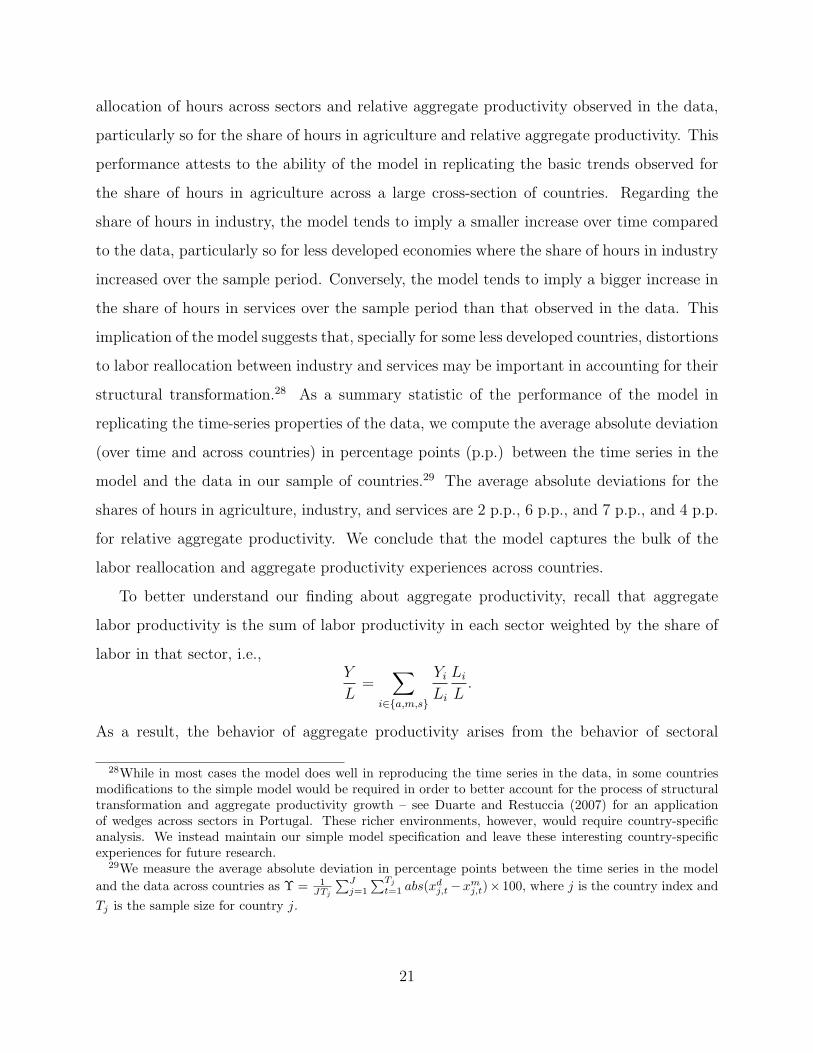
To better understand our finding about aggregate productivity, recall that aggregate

labor productivity is the sum of labor productivity in each sector weighted by the share of

labor in that sector, i.e.,Y

L=

∑i∈{a,m,s}

YiLi

LiL.

As a result, the behavior of aggregate productivity arises from the behavior of sectoral

28While in most cases the model does well in reproducing the time series in the data, in some countriesmodifications to the simple model would be required in order to better account for the process of structuraltransformation and aggregate productivity growth – see Duarte and Restuccia (2007) for an applicationof wedges across sectors in Portugal. These richer environments, however, would require country-specificanalysis. We instead maintain our simple model specification and leave these interesting country-specificexperiences for future research.

29We measure the average absolute deviation in percentage points between the time series in the modeland the data across countries as Υ = 1

JTj

∑Jj=1

∑Tj

t=1 abs(xdj,t−xm

j,t)× 100, where j is the country index andTj is the sample size for country j.

21

labor productivity and the allocation of labor across sectors over time.30 Since the model

reproduces the salient features of labor reallocation across countries, aggregate productivity

growth in the model is also broadly consistent with the cross-country data.

The model has implications for sectoral output in each country. Sectoral output is given

by the product of labor productivity and labor hours. As a result, the growth rate of output

in sector i is the sum of the growth rates of labor productivity Ai (which we take from

the data) and the growth in labor hours Li. The fact that the model reproduces well the

cross-country patterns of the structural transformation implies that sectoral output growth

is also well captured by the model.

The model also has implications for levels and changes over time in relative prices across

countries. We first discuss the implications for changes in relative prices. Figure 9 plots the

annualized percentage change in the prices of agriculture and services relative to manufactur-

ing in the model and the data. The figure shows that the model captures the broad patterns

of price changes in the data – since productivity growth tends to be faster in agriculture

than in industry and in industry than in services in most countries, the tendency is for the

relative price of agriculture to fall and the relative price of services to increase over time.

We note that in the model, the only factors driving price changes over time are the growth

in labor productivity across sectors. Of course, there are many other factors that can drive

price changes over time so the model cannot capture all the changes.

Now we turn to the implications of the model regarding price-level differences across coun-

tries. Recall that the prices of agriculture and services relative to industry are given by the

inverse of labor productivity (Am/Aa, Am/As). The fact that the dispersion in productivity

across rich and poor countries is large in agriculture and services relative to industry implies

that the relative price of agriculture and services are higher in poor relative to rich countries.

These implications may seem at first inconsistent with conventional wisdom about price dif-

ferences across countries. We emphasize however that this conventional wisdom steams from

observations about expenditure prices (often from PWT) instead of producer prices. For

30Note that in the above equation, sectoral labor productivity is measured at a common set of prices acrosscountries.

22

instance, the conventional wisdom is that food is cheap in poor countries. This observation

arises when the PPP-expenditure price of food is compared across countries using market

exchange rates. But when the price of food is compared relative to other goods, food appears

expensive in poor countries (see Summers and Heston (1991), page 338). Moreover, food

expenditures include distribution and other charges and the distinction between producer

and expenditure prices may differ systematically across countries.31 In fact, producer-price

data reveals an even more striking conclusion about the price of agriculture across countries:

the evidence from FAO is that prices of agricultural goods are much higher in poor than

in rich countries. This evidence is consistent with our findings that labor productivity in

agriculture is lower in poor relative to rich countries.

Related is the conventional wisdom that the price of services is higher in rich relative to

poor countries. This view steams again from observations about expenditure prices that may

include a host of distortions that differ across countries (see Summers and Heston (1991)

pages 338 and 339). While there is no systematic producer-price level data for services that

can be compared with the price implications of the model, we focus instead on the indirect

evidence from productivity measurements found in micro studies. Since the lower relative

price of services in rich countries in the model steams from a higher relative productivity in

services than in manufacturing compared to poor countries, we can use the available pro-

ductivity measurements to indirectly assess the price implications of the model for services.

The evidence suggests that labor productivity differences between rich and poor countries

in services are larger than that of manufacturing industries as discussed by Baily and Solow

(2001) from the McKinsey studies and other OECD studies discussed earlier. This evidence

is consistent with our productivity findings and therefore with the price implications of the

model. To summarize, while the lack of systematic price-level data prevents a definite con-

clusion about relative price differences across countries, the available evidence is consistent

with the sectoral productivity findings and their price-level implications in the model.

31In the United States for instance, for every dollar expended on food, only 20 cents go to the farmer forthe agricultural products.

23

4.3 Counterfactuals

We construct a series of counterfactuals aimed at assessing the quantitative importance of

sectoral labor productivity on the process of structural transformation and aggregate pro-

ductivity experiences across countries. We focus on two sets of counterfactuals. The first set

is designed to illustrate the mechanics of positive sectoral productivity growth for labor real-

location and the contribution of productivity growth differences across sectors and countries

for labor reallocation and aggregate productivity. The second set of counterfactuals focuses

on explaining aggregate productivity growth experiences of catch-up, slowdown, stagnation,

and decline by assessing the contribution of specific cross-country sectoral productivity pat-

terns such as productivity catch-up in agriculture and industry and low productivity levels

and the lack of catch-up in services.

4.3.1 The Mechanics of Sectoral Productivity Growth

We consider counterfactuals where in each case we set the growth rate of labor productivity

in a sector to zero in all countries leaving the remaining growth rates as in the data. These

counterfactuals illustrate the importance of productivity growth in each sector for labor

reallocation and aggregate productivity. Summary statistics for these counterfactuals are

reported in Table 2 and Figure 10. The statistics reported are the change between the

last and first periods (in percentage points) in the time series of the share of hours in each

sector and relative aggregate productivity. We start with the counterfactual for agriculture

(γa = 0). No productivity growth in agriculture generates no labor reallocation away from

agriculture: there is an average increase in the share of hours in agriculture of 2 percentage

points (p.p.) in the counterfactual instead of a decrease of 26 p.p. in the model. As a

result, much less labor is reallocated to services. This counterfactual has important negative

implications for relative aggregate productivity for most countries regardless of their level of

development: there is an average decline in relative aggregate productivity of 1 p.p. in the

counterfactual instead of the 13 p.p. increase in the model. The effect of the counterfactual

on labor reallocation implies that agriculture represents a larger share of labor than in the

model. As a result, the negative impact of no growth in agriculture on aggregate productivity

24

is magnified by the endogenous response of labor. Similarly, positive productivity growth in

agriculture moves labor away from agriculture which dampens the positive impact of growth

in this sector on aggregate productivity gains.

Next we turn to the counterfactual for industry (γm = 0). This counterfactual has no

effect on the share of hours in agriculture (see equation 7). With no productivity growth in

industry there is much less reallocation of labor away from industry into services compared

to the model and thus industry represents a larger share of output in the counterfactual.

As before, the negative impact of no growth in industry on aggregate productivity is mag-

nified by the endogenous response of labor. The result is a process for relative aggregate

productivity that is sharply diminished across countries: an average decline of 7 p.p. in the

counterfactual instead of the catch-up of 13 p.p. in the model. An indeed the largest negative

impact is on countries that observed the most catch-up in relative aggregate productivity in

the model. Finally, no productivity growth in services (γs = 0) has a very small impact on

labor reallocation across sectors.32 Relative aggregate productivity declines by an average

of 2 p.p. in this counterfactual. Note that the negative impact of this counterfactual on

relative aggregate productivity is smaller than that of the case with no productivity growth

in industry for all countries but three (Japan, Portugal, and Venezuela) even though services

account for a larger share of hours than industry in most countries.

In the next counterfactual we assess the quantitative importance of differences in labor

productivity growth across sectors and countries on aggregate productivity. We set labor

productivity growth in each sector to the growth rate of aggregate labor productivity in

the United States. The forth column in Figure 10 (γi = γUS) documents the results of this

counterfactual for all countries in the sample. (See also Table 2.) The counterfactual has

a substantial impact on the process of structural transformation. In particular, much less

labor is reallocated away from agriculture and industry towards services. For instance, over

the sample period the share of hours in agriculture fell on average 26 p.p. in the model

and 17 p.p. in the counterfactual. In turn, the share of hours in services increased on

32This is due to two opposing effects of productivity growth in services on the labor allocation betweenindustry and services which roughly cancel each other in the model. See Duarte and Restuccia (2007), page42, for a detailed discussion of these effects.

25

average 36 p.p. in the model and 22 p.p. in the counterfactual. And indeed this different

reallocation process together with the assumption about sectoral labor productivity growth

explains a large portion of the experiences of catch-up and decline in aggregate productivity.

For countries that catch-up in aggregate productivity to the United States in the model

over the sample period, the average catch-up is 26 p.p. in the model and only 2 p.p. in the

counterfactual. For countries that declined in relative aggregate productivity in the model

over the sample period, the average decline is 11 p.p. in the model and only 2 p.p. in the

counterfactual.33

We conclude from these counterfactuals that sectoral productivity growth generates sub-

stantial effects on labor reallocation which in turn are important in understanding aggregate

productivity growth across countries.

4.3.2 Sectoral Productivity Patterns and Cross-Country Experiences

We now turn to the second set of counterfactuals where we assess the role of specific la-

bor productivity patterns across sectors in explaining cross-country episodes of catch-up,

slowdown, stagnation, and decline in relative aggregate productivity. As we documented

in Figure 6, there has been a substantial catch-up in labor productivity in agriculture and

industry across countries. To assess the importance of this sectoral catch-up for aggregate

productivity we compute a set of counterfactuals were in each case we set the growth rate of

labor productivity in a sector to the growth rate in that sector in the United States leaving

the other sectors’ growth rates as in the data (γi = γUSi for each i ∈ {a,m, s}). For com-

pleteness we also compute a counterfactual were all sectoral growth rates are set to the ones

in the United States (γi = γUSi ∀i). Table 3 summarizes the results for these counterfactuals.

While there has been substantial catch-up of labor productivity in agriculture during the

sample period (from an average relative productivity of 48 percent in the first period to 71

33Notice that this counterfactual does not eliminate all aggregate productivity growth differences acrosscountries even though productivity growth rates are identical across sectors and countries and labor reallo-cation is much diminished as a result. For instance, in the counterfactual, relative aggregate productivity inFinland increases by 8 p.p. over the sample period and it decreases by 6 p.p. in Mexico. These movements inrelative aggregate productivity in the counterfactual stem solely from labor reallocation across sectors (dueto positive productivity growth) that have different labor productivity levels.

26

percent in the last period of the sample), this factor contributes little, about 10 percent, to

catch-up in aggregate productivity across countries (1.3 p.p. of 12.8 p.p. in the model). The

substantial catch-up in agricultural productivity produces a reallocation of labor away from

this sector which dampens its positive effect on aggregate productivity growth.

Substantial has also been the catch-up in industry productivity. Unlike agriculture, this

catch-up has a significant impact on relative aggregate productivity. Given that most coun-

tries have observed higher growth rates of labor productivity in industry than the United

States, labor reallocation away from industry and toward services is diminished in the coun-

terfactual for industry. On average, the share of hours in industry decreases 6.5 p.p. in the

counterfactual compared to a decrease of 10.3 p.p. in the model. Figure 11 summarizes our

findings for the effect of this counterfactual on relative aggregate productivity by reporting

the difference in relative aggregate productivity between the last and the first period in the

time series for each country. Industry productivity growth is important for countries that

catch-up in aggregate productivity to the United States since these countries are substan-

tially below the 45-degree line. In fact, we draw in this figure a dash-dotted line indicating

half the gains in aggregate productivity in the counterfactual relative to the model. Many

countries are in this category and some countries substantially below it such as Australia,

Sweden, and the United Kingdom. For all countries, the average change in relative aggre-

gate productivity is only 6 p.p. in the counterfactual instead of 12.8 p.p. in the model.34 We

conclude from this counterfactual that productivity catch-up in industry explains about 50

percent (6.8 p.p. of 12.8 in the model) of the relative aggregate productivity gains observed

during the sample period.

Recall that, in contrast to agriculture and industry, there has been no substantial catch-

up in services across countries and, as reported in Figure 6, there has been a decline in relative

productivity in services for the richer countries. As a result, even though services represent

an increasing share of output in the economy, we do not expect services to contribute much to

catch-up in the model. This is confirmed in the third counterfactual as productivity catch-up

34Note that among countries that decline in relative productivity the effect of industry growth is notsystematic and the gaps are not as large.

27

in services contributes about 15 percent of the catch-up in relative aggregate productivity

(2.4 p.p. of 12.8 p.p. in the model). We note however that for countries that decline in

relative aggregate productivity, lower growth in services than in the United States contributes

substantially to this decline (-6.8 p.p. of -10.5 p.p. in the model, see Table 3). Among

the developed economies – which feature a large share of hours in services – only Canada,

New Zealand, and Sweden had lower productivity growth rates in services than the United

States. In the model, Canada and New Zealand decline in relative aggregate productivity

by 9 and 8 p.p. over the sample period, while Sweden observed a substantial catch-up in

relative aggregate productivity but stagnated at around 82 percent during the mid-1970s.

In the counterfactual, relative aggregate productivity increases by 3 p.p. in Canada, remains

constant for New Zealand, and increases by 9 p.p. from the stagnated level in Sweden. Low

productivity growth in services is essential for understanding these growth experiences of

stagnation and decline among rich economies.

Recall also from Figure 6 that the level of relative productivity in services is lower than

that of industry and that most countries failed to catch-up in services to the relative level

of industry. For instance, the average relative productivity in services increased from 46

percent in the first period to 49 percent in the last period in the sample, whereas the average

relative productivity in industry increased from 51 percent to 75 percent. In the last period

of the sample, all countries except Austria, France, Denmark, the United Kingdom, and

New Zealand feature lower relative productivity in services than in industry. Moreover, in

many instances the differences in productivity between services and industry are substantial:

around 40 percent lower in services in Spain, Finland, and Norway, around 60 percent lower

in Portugal, and around 80 percent lower in Korea and Ireland. These features imply that

the service sector represents an increasing drag on aggregate productivity as resources are

reallocated to this sector in the process of structural transformation. To illustrate the role of

low productivity in services and the lack of catch-up in accounting for the growth experiences

of slowdown, stagnation, and decline, we compute a counterfactual where we let productivity

growth in services be such that in the last period in the sample relative productivity in

services is the same as relative productivity in industry in each country. While the impact

28

of these different productivity growth rates in services on labor reallocation is somewhat

limited, the impact on growth experiences across countries is quite striking: for countries

that catch-up to the United States during the sample period, the average catch-up increases

by almost 80 percent to 46 p.p. while for countries that decline there is instead a catch-

up of 1.6 p.p. during the sample period (see Table 3). More importantly, these summary

statistics hide the impact of productivity in services in explaining experiences of slowdown,

stagnation, and decline observed in the time series. For this reason, Figure 12 plots the time

path of relative aggregate productivity for all country experiences of slowdown, stagnation,

and decline in relative aggregate productivity. The solid lines represent the model and

the dash-dotted lines represent the counterfactual. This figure clearly indicates the extent

to which low productivity in services and the lack of catch-up accounts for all these poor

growth experiences.

To summarize, while productivity convergence in industry (and agriculture) are essential

in the first stages of the process of structural transformation, the poor relative performance

in services has determined a slowdown, stagnation, and decline in aggregate productivity.

In fact, in the last period of the sample, almost all countries observe a lower relative labor

productivity in services than in aggregate (see Figure 13). Since growth rate differences

across countries in the service sector tend to be small and services represent a large and

increasing share of hours in most countries, this suggests an increasing role of services in

determining cross-country aggregate productivity outcomes.

4.4 Discussion

Our analysis of the structural transformation and aggregate productivity growth relies on a

collection of closed economies. It is of interest to discuss the limitations and implications

of this assumption for the results. Openness and trade can have two main effects in an

economy. First, competition from trade can affect domestic productivity. Second, for a

small open economy prices of traded goods reflect world-market conditions and not domestic

productivity.

Regarding the effect of trade on productivity, we argue that the closed-economy assump-

29

tion is not as restrictive for our analysis as it may first appear. To see this point, notice that

the effect of openness on labor allocations and aggregate productivity is already embedded

in the measures of labor productivity growth by sector which the analysis takes as given. For

instance, we found that the growth rate of labor productivity in manufacturing for Korea

was almost 3 times that of the United States. It is likely that openness to trade during

this period can help explain this fact. Moreover, openness would imply that productivity

differences across countries of those goods that are most tradable would tend to be small

relative to the differences of those goods that are less traded. The productivity implications

of the model are consistent with this broad prediction since differences in manufacturing

productivity are smaller than the productivity differences in services. It is an interesting

question for future research to assess the importance of trade for productivity convergence

in manufacturing across countries and the lack of convergence in services which are mostly

non-traded goods.

Regarding the effect of trade on relative prices, recall that the closed-economy assump-

tion implies a one-to-one mapping from sectoral productivity growth to relative prices. An

open-economy version of the model would tend to produce a weaker link between domestic

productivity growth and relative prices. In fact, in a small-open economy relative prices are

invariant to domestic productivity. As we discussed earlier, the relative price implications

of the model are broadly consistent with the data which suggest that productivity growth

is a substantial component of the movements in relative prices. To put it differently, we

found a strong correlation between changes in relative prices and labor productivity growth

across countries as documented in Figure 9. As a result, the labor allocations implied by the

model are broadly consistent with the incentives that consumers face in these economies. We

found that not all differences in relative prices are captured by the model. In particular, we

found that the price of services relative to manufacturing increased faster in the model than

in the data for many countries. This departure of the model from the data may arise not

only from the closed-economy assumption, but also from other features of the data such as

price distortions and barriers to labor reallocation across sectors. It is an interesting ques-

tion why prices of tradable goods are not equalized across countries. The evidence suggests

30

large departures from the law of one price. For instance, the price exercise from FAO on

agricultural goods suggests large price differences across countries (see Prasada Rao (1993))

and the international macro literature documents large deviations in prices even for highly

tradable goods.

Another potential avenue to assess the limitations of the closed-economy assumption of

the model would be to compare the consumption and production implications relative to

data. For instance, in the closed economy output and consumption shares are equal, but

in the open economy they would differ. Unfortunately, this implication cannot be tested

directly since consumption is measured as expenditures in final goods and any gap between

production and consumption of goods may be due to processing, distribution and marketing

services and other charges. But since for the more developed countries most of the trade oc-

curs intra-industry – different cars or wines are shipped to and from countries – consumption

and production shares of broad sectors would tend not to differ greatly in a country.

5 Conclusions

We documented the reallocation of labor over time between agriculture, industry, and services

and the growth of sectoral labor productivity across countries. While countries are going

through a common process of structural transformation, we found that there is substantial

lag differences in this process. We also found that most countries tend to observe low

productivity growth in services compared to agriculture or manufacturing even though there

is a big variation in sectoral labor productivity growth across countries.

Using a model of the structural transformation that is calibrated to the growth experi-

ence of the United States, we showed that sectoral differences in labor productivity levels

and growth explain the broad patterns of the process of structural transformation and ag-

gregate productivity experiences across countries. We found that sectoral labor productivity

differences across countries are large and systematic both at a point in time and over time.

In particular, labor productivity differences between rich and poor countries are large in

agriculture and services and smaller in manufacturing. Moreover, most countries have ex-

31

perienced substantial productivity catch-up in agriculture and industry but productivity in

services has remained low relative to the United States. An implication of these findings is

that, as countries move through the process of structural transformation, relative aggregate

labor productivity can first increase (as labor moves from agriculture to industry) and later

stagnate or decline (as labor moves from agriculture and industry to services). We find that

sectoral productivity differences can account for the bulk of differences in the process of

structural transformation and aggregate productivity experiences across countries.

This paper highlights the role of sectoral labor productivity differences for the structural

transformation and aggregate productivity experiences across countries. We find that labor

productivity catch-up in manufacturing explains about 50 percent of the gains in aggregate

productivity across countries and that low labor productivity in services and the lack of catch-

up explains all the experiences of slowdown, stagnation, and decline in relative aggregate

productivity across countries. Thus, understanding the sources of cross-country differences

in labor productivity levels and growth across sectors is crucial. In analyzing sectoral labor

productivity levels and growth rates across countries, a number of interesting questions arise.

What factors contribute to cross-country differences in labor productivity across sectors?

Why were countries able to catch-up in manufacturing productivity but not in services?

What are the barriers that prevent other developed economies to sustain growth rates of

labor productivity in services as high as in the United States? How are trade openness and

regulation related to these productivity differences across countries?

While there may not be a unifying explanation for all these observations, a recurrent

theme in productivity studies at the sectoral level is that the threat or actual pressure of

competition is crucial for productivity performance, see for instance Schmitz (2005) and

Galdon-Sanchez and Schmitz (2002). Since services are less traded than manufacturing

goods, there is a tendency for services to be less subject to competitive pressure and this

may explain the larger productivity gaps in services relative to manufacturing across coun-

tries. Moreover, protected domestic industries may be the explanation to poor productivity

performance in some countries. Since openness to trade would not generally have the desired

competitive-pressure impact in services, other factors such as the regulatory environment

32

may prove useful in explaining productivity differences across countries in this sector. Poli-

cies aimed at limiting regulations or government interventions that affect competition and

productivity may explain productivity growth differences in services. For instance, it is often

emphasized the role of land and size regulations affecting productivity in retail services, see

for instance Baily and Solow (2001). As a first pass in providing some empirical support

for this potential explanation to productivity differences across countries, we have correlated

labor productivity differences in industry and services derived from our model to measures

of trade openness and government regulation. We find that trade openness is strongly cor-

related to industry productivity but less so with services productivity, while measures of

regulation (such as that from the World Bank’s Doing Business) are strongly correlated with

productivity in services. We leave a detailed investigation of these important issues for future

research.

33

References

Adamopoulos, T. and Akyol, A. (2007) “Relative Underperformance Alla Turca,” Review ofEconomic Dynamics, forthcoming.

Baily, M., Farrell, D., and Remes, J. (2005) “Domestic Services: The Hidden Key toGrowth,” McKinsey Global Institute.

Baily, M. and Solow, R. (2001) “International Productivity Comparisons Built from the FirmLevel,” Journal of Economic Perspectives, 15(3): pp. 151-172.

Banco de Portugal (2006) “Series Longas para a Economia Portuguesa pos II GuerraMundial.” Available online:<http://www.bportugal.pt/publish/serlong/serlong p.htm.>

Baumol, W. (1967) “Macroeconomics of Unbalanced Growth: The Anatomy of Urban Cri-sis,” American Economic Review, 53(3): pp. 415-26.

Caselli, F. (2005) “Accounting for cross-country income differences,” in: Aghion, P., Durlauf,S. N. (Eds.), Handbook of Economic Growth, Vol. 1A. North Holland Elsevier, New York,NY, pp. 679-741.

Caselli, F. and Coleman, W. J. (2001) “The U.S. Structural Transformation and RegionalConvergence: A Reinterpretation,” Journal of Political Economy, 109: pp. 584-616.

Caselli, F. and Tenreyro, S. (2006) “Is Poland the Next Spain?,” NBER International Sem-inar on Macroeconomics 2004, Richard Clarida, Jeffrey Frankel, Francesco Giavazzi, andKenneth West, editors. The MIT Press, pp. 459-523.

Chanda, A. and Dalgaard, C.J. (2005) “Dual economies and international total factor pro-ductivity differences,” Working Paper 2005-11, Department of Economics, Louisiana StateUniversity.

Chari, V.V., Kehoe, P., and McGrattan, E. (1996) “The Poverty of Nations: A QuantitativeExploration,” NBER Working Paper 5414.

Coleman, J. W. (2007) “Accommodating Emerging Giants,” manuscript, Duke University.

Conference Board and Groningen Growth and Development Centre (2008a), Total EconomyDatabase, http://www.conference-board.org/economics/.

Conference Board and Groningen Growth and Development Centre (2008b), 10-SectorDatabase, http://www.conference-board.org/economics/.

Cordoba, J. and Ripoll, M. (2004) “Agriculture, Aggregation, and Development Accounting,”manuscript, University of Pittsburgh.

Duarte, M. and Restuccia, D. (2006) “The Productivity of Nations,” Federal Reserve Bankof Richmond Economic Quarterly, 92(3): pp. 195-223.

34

Duarte, M. and Restuccia, D. (2007) “The Structural Transformation and Aggregate Pro-ductivity in Portugal,” Portuguese Economic Journal, 6(1): pp. 23-46.

Echevarria, M. (1997) “Changes in Sectoral Composition Associated with Growth,” Inter-national Economic Review, 38: pp. 431-52.

EUKLEMS Database (2008), see Timmer, M, O’Mahony, M., and van Ark, B. “The EUK-LEMS Growth and Productivity Accounts: An Overview”, University of Groningen andUniversity of Birmingham; downloadable at www.euklems.net.

Galdon-Sanchez, J. and Schmitz Jr., J. (2002) “Competitive Pressure and Labor Produc-tivity: World Iron-Ore Markets in the 1980’s,” American Economic Review 92(4): pp.1222-1235

Gollin, D., Parente, S., and Rogerson, R. (2002) “The Role of Agriculture in Development,”American Economic Review Papers and Proceedings, 92(2): pp. 160-164.

Gollin, D., Parente, S., and Rogerson, R. (2007) “The Food Problem and the Evolution ofInternational Income Levels,” Journal of Monetary Econmics, 54(4): pp. 1230-1255.

Hansen, G. and Prescott, E. C. (2002) “From Malthus to Solow,” American Economic Re-view, 92(4): pp. 1205-1217.

Herrendorf, B. and Valentinyi, A. (2006) “Which Sectors Make the Poor Countries so Un-productive?,” manuscript, Arizona State University.

Heston, A., Summers, R., and Atten, B. (2006) Penn World Table Version 6.2, Center forInternational Comparisons of Production, Income and Prices at the University of Penn-sylvania, September, <http://pwt.econ.upenn.edu>.

International Labour Office (2008), LABORSTA Database, Bureau of Statistics,<http://laborsta.ilo.org/>.

Jones, C. (1997) “On the Evolution of the World Income Distribution,” Journal of EconomicPerspectives, 11: pp. 19-36.

Kehoe, T. and Prescott, E. C. (2002) “Great Depressions of the 20th Century,” Review ofEconomic Dynamics 5: pp. 1-18.

Kongsamut, P., Rebelo, S., and Xie, D. (2001) “Beyond Balanced Growth,” Review of Eco-nomic Studies, 68: pp. 869-882.

Kuznets, S. (1966) Modern Economic Growth, Yale University Press.

Laitner, J. (2000) “Structural Change and Economic Growth,” Review of Economic Studies,67: pp. 545-61.

Lucas, R. (2000) “Some Macroeconomics for the 21st Century,” Journal of Economic Per-spectives, 14: pp. 159-168.

35

Maddison, A. (1980) “Economic Growth and Structural Change in the Advanced Countries,”in Western Economies in Transition, eds.: I. Leveson and W. Wheeler. London: CroomHelm.

Ngai, L. R. (2004) “Barriers and the Transition to Modern Growth,” Journal of MonetaryEconomics, 51(7): pp. 1353-1383.

Ngai, L. R. and C. A. Pissarides (2007) “Structural Change in a Multi-Sector Model ofGrowth,” American Economic Review, 97(1): pp. 429-443.

OECD Database (2008), Labor Force Statistics online, Source OECD: Outlooks & Annuals(1960-2004), available on-line<http://hermia.sourceoecd.org/vl=718832/cl=16/nw=1/rpsv/outlook annuals.htm.>

OECD Corporate Data Environment (1956-2003), “Labor Force Statistics Database.” Avail-able online:<http://www1.oecd.org/scripts/cde/members/lfsdataauthenticate.asp.>

OECD Publications. “National Accounts of OECD Countries,” (Detailed Tables, Volume II,1950-1961 and 1960-1977).

Pilat, D. (1996) “Labour Productivity Levels in OECD Countries: Estimates for Manufac-turing and Selected Service Sectors,” OECD Working Paper 169.

Prasada Rao, D.S. (1993) “Intercountry Comparisons of Agricultural Output and Produc-tivity,” FAO Economic and Social Development Paper No. 112. Food and AgricultureOrganization of the United Nations.

Prescott, E. C. (2002) “Prosperity and Depression,” American Economic Review, 92(2): pp.1-15.

Restuccia, D., Yang, D., and Zhu, X. (2008) “Agriculture and Aggregate Productivity: AQuantitative Cross-Country Analysis,” Journal of Monetary Economics, 55: pp. 234-250.

Rogerson, R. (2008) “Structural Transformation and the Deterioriation of European LaborMarket Outcomes,” Journal of Political Economy, 116(2): pp. 235-259.

Schmitz, J. (2005) “What Determines Productivity? Lessons from the Dramatic Recovery ofthe U.S. and Canadian Iron Ore Industries Following Their Early 1980s Crisis”, Journalof Political Economy 113(3): pp. 582-625.

Summers, R. and Heston, A. (1991) “The Penn World Table: an expanded set of internationalcomparisons, 1950-1988”, Quarterly Journal of Economics 106: pp. 327-68.

U.S. Census Bureau, Department of Commerce. Historical Statistics of the United States:Colonial Times to 1970 (Part I). Washington, DC: U.S. Government Printing Office, 1975.

36

Vollrath, D. (2009) “How Important are Dual Economy Effects for Aggregate Productivity?”Journal of Development Economics 88: pp. 325-34.

World Bank (2008). World Development Indicators. Available on-line:<http://devdata.worldbank.org/dataonline/>.

37

A Data Sources and Definitions

We build a panel data set with annual observations for aggregate GDP per hour, andvalue added per hour and shares of hours for agriculture, industry, and services for 29countries. The countries covered in our data set are, with sample period in parenthesis,Argentina (1950-2004), Australia (1964-2004), Austria (1960-2004), Belgium (1956-2004),Bolivia (1950-2002), Brazil (1950-2003), Canada (1956-2004), Chile (1951-2004), Colombia(1950-2003), Costa Rica (1950-2002), Denmark (1960-2004), Finland (1959-2004), France(1969-2003), Greece (1960-2004), Ireland (1958-2004), Italy (1956-2004), Japan (1960-2004),Korea (1972-2003), Mexico (1950-2004), Netherlands (1960-2004), New Zealand (1971-2004),Norway (1956-2004), Portugal (1956-2004), Spain (1960-2004), Sweden (1960-2004), Turkey(1960-2003), United Kingdom (1956-2004), United States (1956-2004), and Venezuela (1950-2004).

All series are trended using the Hodrick-Prescott filter with a smoothing parameter λ =100 before any ratios are computed.

A.1 Aggregate Data

We obtain data on PPP-adjusted real GDP per capita in constant prices (RGDPL) andpopulation (POP ) from Penn World Tables version 6.2., see Heston, Summers, and Atten(2006); and we obtain data on employment (EMP ) and annual hours actually worked perperson employed (HOURS) from the Total Economy Database, see Conference Board andGroningen Growth and Development Center (2008a). With these data we construct annualtime series of PPP-adjusted GDP per hour in constant prices for each country as Y Lh =RGDPL× POP/(EMP ×HOURS).

A.2 Sectoral Data

We obtain annual data on employment, hours worked, and constant domestic-price valueadded for agriculture, industry, and services for the countries listed above. The sectors aredefined by the International Standard Industrial Classification, revision 3 (ISIC III) defini-tions, with agriculture corresponding to ISIC divisions 1-5 (agriculture, forestry, hunting,and fishing), industry to ISIC divisions 10-45 (mining, manufacturing, construction, elec-tricity, water, and gas), and services to ISIC divisions 50-99 (wholesale and retail trade– including hotels and restaurants, transport, and government, financial, professional, andpersonal services such as education, health care, and real estate services).

A.2.1 Value Added by Sector

Value added by sector is obtained by combining data from the World Bank (2008), WorldDevelopment Indicators online and historical data from the OECD National Accounts publi-cations for the following countries: Australia, Austria, Belgium, Canada, Denmark, Finland,France, Greece, Ireland, Italy, Japan, Korea, Netherlands, New Zealand, Norway, Portugal,Spain, Sweden, Turkey, United Kingdom, and United States.

38

The data series from the World Bank’s World Development Indicators are agriculturevalue added, industry value added, and services value added. All series are measured inconstant local currency units, base year 2000 (with the exception of Turkey, 1987). Theseseries are extended backwards using historical data from the OECD National Accounts pub-lications, except for Korea. A combination of three OECD publications was used: NationalAccounts of OECD Countries (1950-1968), National Accounts of OECD Countries (1950-1961), and National Accounts of OECD Countries (1960-1977). The primary resource wasthe book covering the period from 1950 to 1968. We compute growth rates of the OECDdata for corresponding variables for years prior to those available through the World Bankand apply them to the World Bank series.

Data on value added by sector for all Latin American countries in our data set (Argentina,Bolivia, Brazil, Chile, Colombia, Costa Rica, Mexico, and Venezuela) are obtained from the10-Sector Database (see Conference Board and Groningen Growth and Development Center(2008b)). This database has data on value added in constant local prices for 10 sectors.These data are aggregated into value added in agriculture, industry, and services using theISIC III definitions above.

A.2.2 Employment by Sector

The sectoral employment data is obtained from a variety of sources as well. We obtain dataon civilian employment in each broad sector from OECD databases (Labor Force Statistics,Main Economic Indicators, and Annual National Accounts) for: Australia, Austria, Belgium,Canada, Finland, France, Ireland, Italy, Japan, Netherlands, New Zealand, Norway, Spain,Turkey, United Kingdom, and United States. Data for Portugal on sectoral employmentis obtained from the Banco de Portugal (2006). The data is aggregated into the samethree broad sectors. We extend this series forward to 2005 by using growth rates for eachvariable computed from EUKLEMS Database (2008). Data for Korea and all Latin Americancountries is obtained from the 10-Sector Database (see Conference Board and GroningenGrowth and Development Center (2008b)). We aggregate this data into the three broadsectors using the ISIC III definitions above.

A.2.3 Hours Worked by Sector

We obtain data on hours of work per worker from the EUKLEMS Database (2008) for Aus-tralia, Austria, Belgium, Denmark, Finland, France, Ireland, Italy, Japan, the Netherlands,Portugal, Spain, Sweden, United Kingdom, and United States. This data cover the period1970 to 2005. Data for Brazil, Canada, Chile, Colombia, Costa Rica, Greece, Mexico, Nor-way, New Zealand, and Turkey is obtained from International Labour Office (2008), Laborstadatabase. These series are much shorter; the time period covered varies by country but itstarts after 1990 for all countries.

From these data, we compute the ratio of per-worker hours by sector relative to per-worker aggregate hours. In analyzing these ratios, we find that relative sectoral hours areremarkably stable over time for most countries and that these ratios are very close to onefor many countries. Moreover, any deviations from one in relative hours across countries

39

are not systematically related to the level of development. For each country, we use theaverage value of each of these ratios, denoted as hi, i = a,m, s, to calculate shares of hoursby sector and value added per hour by sector. Since the time series of sectoral hours areshorter than those of sectoral employment and value added, this simplification allows us tocompute sectoral shares of total hours and value added per hour without shortening the timeseries. We do not have data on sectoral hours for Argentina, Bolivia, Korea, and Venezuelaand we assume that hi = 1 for these countries.

Total hours by sector are computed by multiplying employment with hours per workerin each sector. We construct value added per hour by dividing the series of value added withthe corresponding series of total hours for each sector. Shares of hours by sector are simplythe ratio of total hours by sector relative to total aggregate hours.

A.2.4 Prices by Sector

We compute implicity price deflators for each sector using data on sectoral value addedat constant and current prices from the World Development Indicators. The price data isconsistent with the sectoral definitions for labor productivity. It covers the period from 1971to 2004.

40

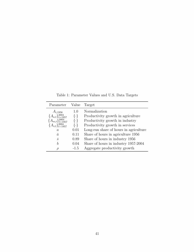
Table 1: Parameter Values and U.S. Data Targets

Parameter Value Target

Ai,1956 1.0 Normalization{Aa,t}2004

t=1957 {·} Productivity growth in agriculture{Am,t}2004

t=1957 {·} Productivity growth in industry{As,t}2004

t=1957 {·} Productivity growth in servicesa 0.01 Long-run share of hours in agriculturea 0.11 Share of hours in agriculture 1956s 0.89 Share of hours in industry 1956b 0.04 Share of hours in industry 1957-2004ρ -1.5 Aggregate productivity growth

41

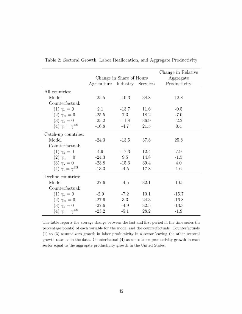
Table 2: Sectoral Growth, Labor Reallocation, and Aggregate Productivity

Change in RelativeChange in Share of Hours Aggregate

Agriculture Industry Services Productivity

All countries:Model -25.5 -10.3 38.8 12.8Counterfactual:

(1) γa = 0 2.1 -13.7 11.6 -0.5(2) γm = 0 -25.5 7.3 18.2 -7.0(3) γs = 0 -25.2 -11.8 36.9 -2.2(4) γi = γUS -16.8 -4.7 21.5 0.4

Catch-up countries:Model -24.3 -13.5 37.8 25.8Counterfactual:

(1) γa = 0 4.9 -17.3 12.4 7.9(2) γm = 0 -24.3 9.5 14.8 -1.5(3) γs = 0 -23.8 -15.6 39.4 4.0(4) γi = γUS -13.3 -4.5 17.8 1.6

Decline countries:Model -27.6 -4.5 32.1 -10.5Counterfactual:

(1) γa = 0 -2.9 -7.2 10.1 -15.7(2) γm = 0 -27.6 3.3 24.3 -16.8(3) γs = 0 -27.6 -4.9 32.5 -13.3(4) γi = γUS -23.2 -5.1 28.2 -1.9

The table reports the average change between the last and first period in the time series (inpercentage points) of each variable for the model and the counterfactuals. Counterfactuals(1) to (3) assume zero growth in labor productivity in a sector leaving the other sectoralgrowth rates as in the data. Counterfactual (4) assumes labor productivity growth in eachsector equal to the aggregate productivity growth in the United States.

42

Table 3: Change in Relative Aggregate Productivity

All Catch-up Declinecountries countries countries

Model 12.8 25.8 -10.5Counterfactual:

(1) γi = γUSi

(1a) Agriculture 11.5 23.2 -9.4(1b) Industry 6.0 13.9 -8.4(1c) Services 10.4 18.3 -3.7

(2) γi = γUSi ∀i 3.9 5.8 0.5

(3) Catch-up in Services 30.7 46.9 1.6

The table reports the average change between the last and first period in the time series (inpercentage points) of relative aggregate productivity for the model and the counterfactuals.Counterfactuals (1a) to (1c) set the growth rate in a sector to the rate in the United Statesin that sector. Counterfactual (2) sets the growth rate of all sectors to the sectoral growthrates in the United States. Counterfactual (3) sets the productivity growth in services suchthat in the last period in the sample relative productivity in services is the same as relativeproductivity in industry in each country.

43

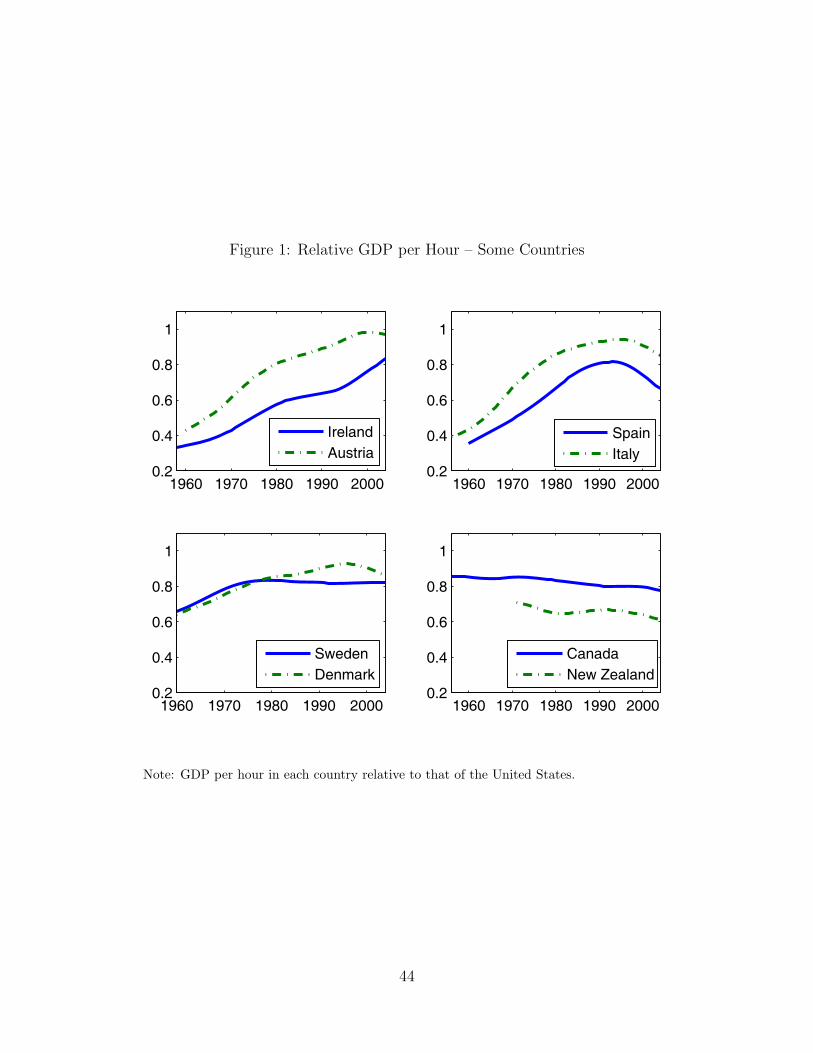
Figure 1: Relative GDP per Hour – Some Countries

1960 1970 1980 1990 20000.2

0.4

0.6

0.8

1

IrelandAustria

1960 1970 1980 1990 20000.2

0.4

0.6

0.8

1

SpainItaly

1960 1970 1980 1990 20000.2

0.4

0.6

0.8

1

SwedenDenmark

1960 1970 1980 1990 20000.2

0.4

0.6

0.8

1

CanadaNew Zealand

Note: GDP per hour in each country relative to that of the United States.

44

Figure 2: Shares of Hours – Some Countries

1960 1970 1980 1990 20000

0.2

0.4

0.6

0.8

1Greece

Agriculture

Industry

Services

1960 1970 1980 1990 20000

0.2

0.4

0.6

0.8

1Ireland

1960 1970 1980 1990 20000

0.2

0.4

0.6

0.8

1Spain

1960 1970 1980 1990 20000

0.2

0.4

0.6

0.8

1Canada

45

Figure 3: Sectoral Growth Rates of Labor Productivity (%)

1 1.5 2 2.5 3 3.5 4 4.5 5−2

0

2

4

6

8

ARG AUS

AUTBEL

BOLBRACAN

CHL

COLCRI

DNK ESP

FINFRA

GBRGRC

IRLITA

JPN

KOR

MEX

NLDNOR

NZL

PRTSWE

TURVEN USA

Agr

icul

ture

1 1.5 2 2.5 3 3.5 4 4.5 5−2

0

2

4

6

8

ARGAUS

AUTBEL

BOL

BRACAN CHLCOLCRI

DNK ESPFIN

FRAGBR

GRC

IRL

ITAJPN

KOR

MEX

NLDNOR

NZL

PRTSWETUR

VEN

USA

Indu

stry

1 1.5 2 2.5 3 3.5 4 4.5 5−2

0

2

4

6

8

ARGAUS

AUTBEL

BOLBRACAN CHLCOLCRI

DNK ESPFINFRAGBR GRCIRLITA

JPNKOR

MEX

NLD NORNZL

PRTSWE

TURVEN

USASer

vice

s

Annualized Growth Rate of Aggregate Labor Productivity

Note: Aggregate labor productivity is GDP per hour while sectoral labor productivity isvalue added per hour in each sector. Annualized percentage growth rates during the sampleperiod for each country. The horizontal lines indicate the sectoral growth rates observed inthe United States and the vertical line indicates the aggregate growth rate of the UnitedStates.

46

Figure 4: Share of Hours by Sector - Model vs. U.S. Data

1955 1960 1965 1970 1975 1980 1985 1990 1995 2000 20050

0.1

0.2

0.3

0.4

0.5

0.6

0.7

0.8

Years

Sha

re o

f Hou

rs

Ag. DataAg. ModelInd. DataInd. ModelSvc. DataSvc. Model

47

Figure 5: Relative Labor Productivity across Sectors - first year

1 2 3 4 50

0.5

1

Agr

icul

ture

1 2 3 4 50

0.5

1

Indu

stry

1 2 3 4 50

0.5

1

Ser

vice

s

Quintile of Aggregate Productivity (first year)

Note: Labor productivity relative to the level of the United States.

48

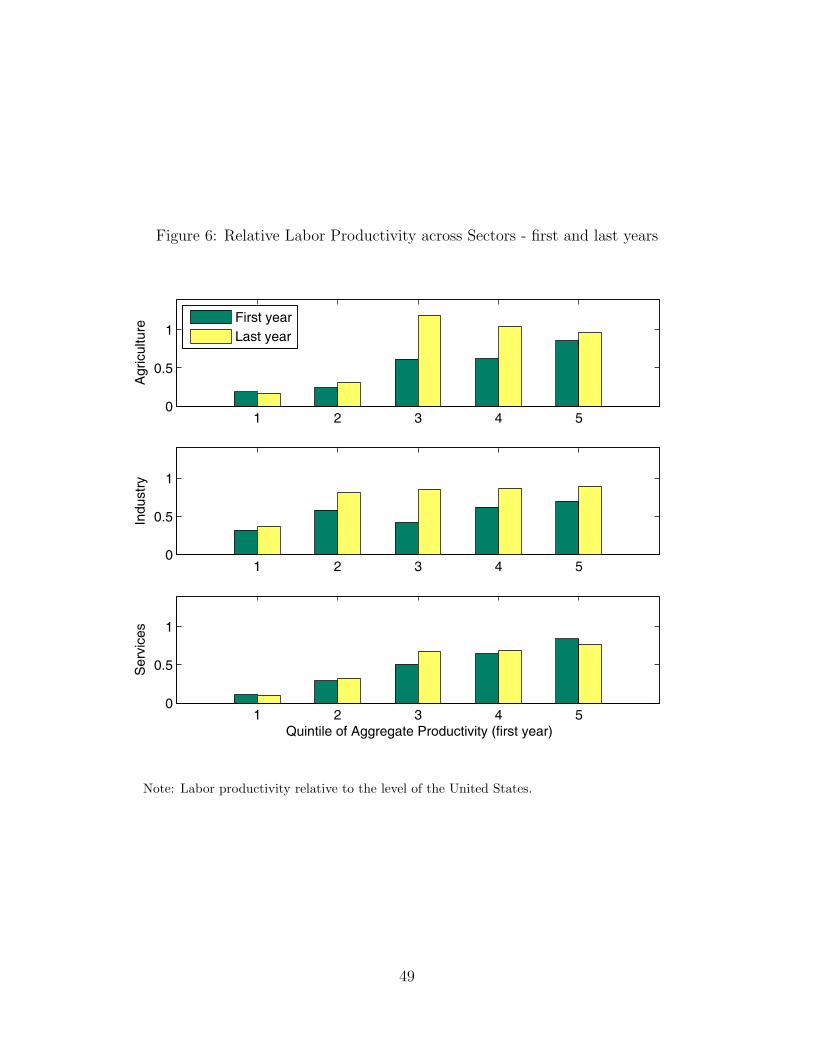
Figure 6: Relative Labor Productivity across Sectors - first and last years

1 2 3 4 50

0.5

1

Agr

icul

ture

First yearLast year

1 2 3 4 50

0.5

1

Indu

stry

1 2 3 4 50

0.5

1

Ser

vice

s

Quintile of Aggregate Productivity (first year)

Note: Labor productivity relative to the level of the United States.

49

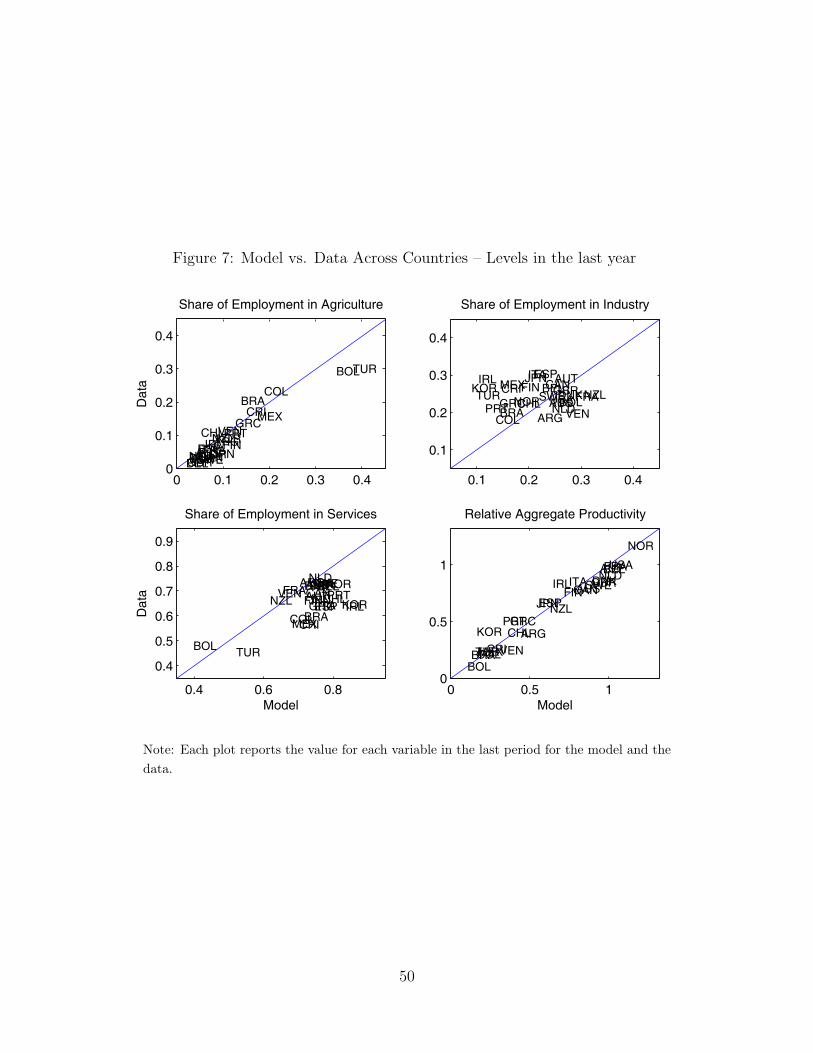
Figure 7: Model vs. Data Across Countries – Levels in the last year

0 0.1 0.2 0.3 0.40

0.1

0.2

0.3

0.4

ARGAUSAUTBEL

BOL

BRA

CAN

CHL

COL

CRI

DNKESP FINFRA

GBR

GRC

IRLITAJPNKOR

MEX

NLDNORNZLPRT

SWE

TUR

VEN

USA

Share of Employment in Agriculture

Dat

a

0.1 0.2 0.3 0.4

0.1

0.2

0.3

0.4

ARGAUS

AUTBEL

BOLBRA

CAN

CHLCOL

CRI DNK

ESPFIN

FRAGBRGRC

IRL ITAJPNKOR MEX

NLDNOR

NZLPRT

SWETUR

VENUSA

Share of Employment in Industry

0.4 0.6 0.8

0.4

0.5

0.6

0.7

0.8

0.9

ARGAUSAUT

BEL

BOL

BRA

CANCHL

COLCRI

DNK

ESPFINFRA GBR

GRC IRLITAJPN KOR

MEX

NLDNORNZL PRT

SWE

TUR

VENUSA

Share of Employment in Services

Dat

a

Model0 0.5 1

0

0.5

1

ARG

AUS

AUTBEL

BOLBRA

CAN

CHL

COLCRI

DNK

ESPFIN

FRAGBR

GRC

IRLITA

JPN

KOR

MEX

NLD

NOR

NZLPRT

SWE

TURVEN

USA

Relative Aggregate Productivity

Model

Note: Each plot reports the value for each variable in the last period for the model and thedata.

50

Figure 8: Model vs. Data Across Countries – Changes

−40 −20 0−50

−40

−30

−20

−10

0

10

ARG

AUSAUT

BEL

BOLBRA

CANCHL

COLCRI

DNK

ESPFIN

FRA

GBR

GRC

IRLITA

JPN

KORMEX

NLD

NOR

NZL

PRT

SWE

TUR

VEN

USA

Share of Hours in Agriculture

Dat

a

−30 −20 −10 0 10 20−30

−20

−10

0

10

20

ARG

AUSAUT

BEL

BOL

BRA

CAN

CHL

COL

CRI

DNK

ESPFIN

FRA

GBR

GRCIRL

ITAJPN

KOR MEX

NLD

NOR NZL

PRT

SWE

TUR

VEN

USA

Share of Hours in Industry

10 20 30 40 50 6010

20

30

40

50

60

ARGAUSAUT

BELBOL

BRA

CAN CHLCOL

CRIDNK

ESPFIN

FRA GBR

GRC

IRL

ITA

JPN

KOR

MEXNLD

NOR

NZL

PRTSWE

TURVENUSA

Share of Hours in Services

Dat

a

Model−40 −20 0 20 40 60

−40

−20

0

20

40

60

ARG

AUS

AUTBEL

BOL

BRA

CANCHLCOL

CRI

DNKESP

FINFRAGBRGRC

IRLITA

JPN

KOR

MEX

NLD

NOR

NZL

PRT

SWETUR

VEN

USA

Relative Aggregate Productivity

Model

Note: Each plot reports the change between the last and first period (in percentage points)of each variable during the sample period in the data and in the model.

51

Figure 9: Changes in Relative Prices (%)

−6 −5 −4 −3 −2 −1 0 1 2 3 4−6

−4

−2

0

2

4

ARG

AUS

AUTBELBOLBRA

CAN

CHL

COLCRI

DNK

ESP

FIN

FRAGBR

GRC

IRL

ITA

JPNKOR

MEX

NLDNOR

NZL

PRT

SWETUR

VEN USA

Relative Price of Agriculture

Dat

a

−3 −2 −1 0 1 2 3 4 5

−2

0

2

4

ARGAUSAUT

BEL

BOL

BRACAN

CHLCOL

CRIDNK

ESP FINFRAGBRGRC

IRL

ITAJPN

KOR

MEX NLD

NOR

NZL

PRT SWE

TUR

VEN

USA

Relative Price of Services

Dat

a

Model

Note: Each figure reports the annualized percentage change of the variable in the time seriesin the data and in the model. Relative price of agriculture and services refer to the price ofagriculture and services relative to industry. Data on relative prices cover the period 1971to 2004.

52

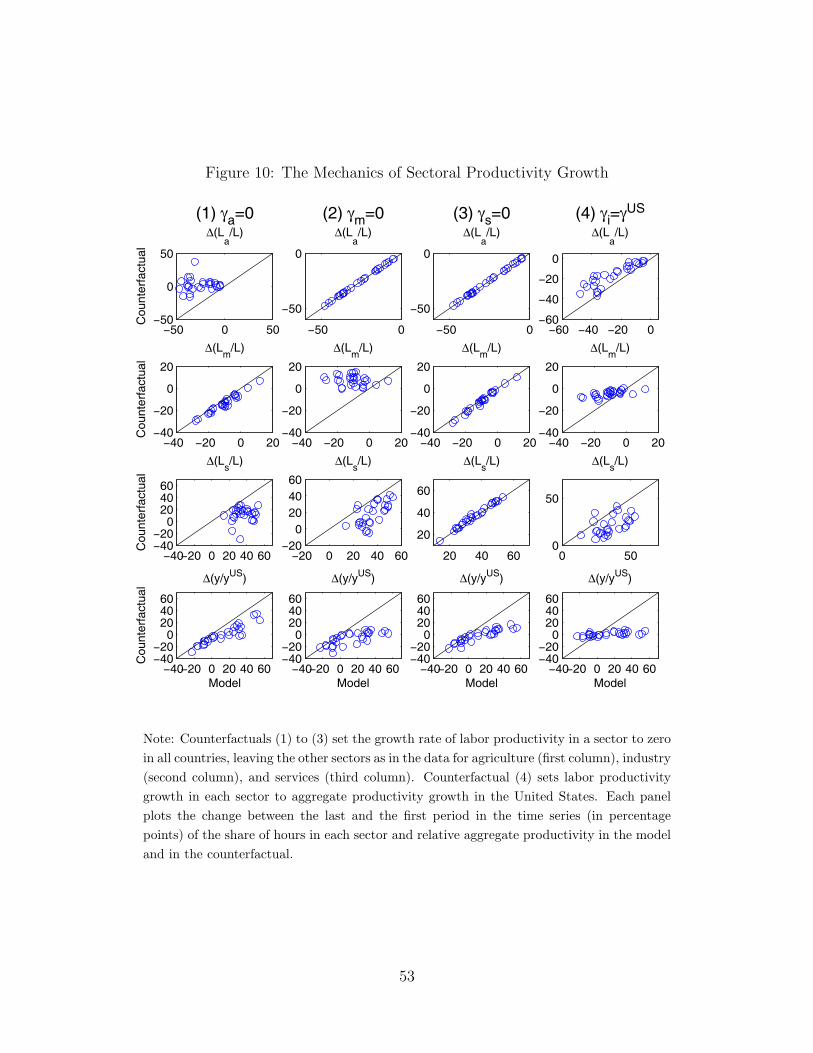
Figure 10: The Mechanics of Sectoral Productivity Growth

−50 0 50−50

0

50

(1) γa=0Δ(L

a/L)

Cou

nter

fact

ual

−40 −20 0 20−40

−20

0

20

Δ(Lm

/L)

Cou

nter

fact

ual

−40−20 0 20 40 60−40−20

0204060

Δ(Ls/L)

Cou

nter

fact

ual

−40−20 0 20 40 60−40−20

0204060

Δ(y/yUS)

Model

Cou

nter

fact

ual

−50 0

−50

0

(2) γm=0Δ(L

a/L)

−40 −20 0 20−40

−20

0

20

Δ(Lm

/L)

−20 0 20 40 60−20

0204060

Δ(Ls/L)

−40−20 0 20 40 60−40−20

0204060

Δ(y/yUS)

Model

−50 0

−50

0

(3) γs=0Δ(L

a/L)

−40 −20 0 20−40

−20

0

20

Δ(Lm

/L)

20 40 60

20

40

60

Δ(Ls/L)

−40−20 0 20 40 60−40−20

0204060

Δ(y/yUS)

Model

−60 −40 −20 0−60

−40

−20

0

(4) γi=γUS

Δ(La/L)

−40 −20 0 20−40

−20

0

20

Δ(Lm

/L)

0 500

50

Δ(Ls/L)

−40−20 0 20 40 60−40−20

0204060

Δ(y/yUS)

Model

Note: Counterfactuals (1) to (3) set the growth rate of labor productivity in a sector to zeroin all countries, leaving the other sectors as in the data for agriculture (first column), industry(second column), and services (third column). Counterfactual (4) sets labor productivitygrowth in each sector to aggregate productivity growth in the United States. Each panelplots the change between the last and the first period in the time series (in percentagepoints) of the share of hours in each sector and relative aggregate productivity in the modeland in the counterfactual.

53

Figure 11: Change in Relative Aggregate Productivity – The Importance of Industry

−20 −10 0 10 20 30 40 50 60

−20

−10

0

10

20

30

40

50

60

ARG

AUS

AUTBEL

BOLBRA

CAN

CHLCOL

CRI

DNKESP

FINFRA

GBRGRC

IRL

ITA

JPN

KOR

MEX

NLD

NOR

NZL

PRTSWE

TUR

VEN

Model

Cou

nter

fact

ual

Note: This counterfactual sets the growth of labor productivity in industry in each countryto the rate in the United States. The figure plots the difference between the last and firstperiod (in percentage points) of relative aggregate productivity during the sample period inthe model and in the counterfactual.

54

Figure 12: Relative Aggregate Productivity – The Importance of Services

1960 1980 2000

0.4

0.5

0.6

0.7

Argentina

1980 2000

0.7

0.8

0.9

1

Australia

1960 1980 20000.7

0.8

0.9

1

Canada

1960 1980 2000

0.3

0.4

0.5

0.6

Chile

1960 1980 2000

0.1

0.2

0.3

0.4Colombia

1960 1980 2000

0.2

0.3

0.4

0.5

Costa Rica

1960 1980 2000

0.4

0.6

0.8

Spain

1960 1980 2000

0.4

0.6

0.8

1

Finland

1960 1980 20000.2

0.4

0.6

Greece

1960 1980 2000

0.4

0.6

0.8

1

Italy

1960 1980 20000.1

0.2

0.3

0.4

Mexico

1960 1980 20000.6

0.8

1

Netherlands

1960 1980 20000.5

1

1.5

Norway

1960 1980 2000

0.2

0.4

0.6

Portugal

1960 1980 20000.6

0.8

1

1.2Sweden

1960 1980 2000

0.1

0.2

0.3

Turkey

Note: This counterfactual sets the productivity growth in services such that in the lastperiod in the sample relative productivity in services is the same as relative productivity inindustry in each country. Each panel plots aggregate labor productivity relative to that ofthe United States in the model and the counterfactual for each country which, during thesample period, experienced an episode of slowdown, stagnation, or decline. The solid linerepresents the model and the dash-dotted line the counterfactual.

55

Figure 13: Labor Productivity in Services across Countries – Last Period

0 0.2 0.4 0.6 0.8 1 1.20

0.2

0.4

0.6

0.8

1

1.2

ARG

AUS

AUT

BEL

BOL BRA

CAN

CHL

COLCRI

DNK

ESP

FIN

FRA

GBR

GRC

IRL

ITA

JPN

KORMEX

NLD

NOR

NZL

PRT

SWE

TUR

VEN

Relative Aggregate Labor Productivity − last year

Rel

ativ

e La

bor

Pro

duct

ivity

in S

ervi

ces −

last

yea

r

Note: This figure plots relative labor productivity in services against relative aggregateproductivity in the last period of the sample for all countries.

56