WP/16/162

From Firm-Level Imports to Aggregate Productivity: Evidence from Korean Manufacturing Firms Data

By JaeBin Ahn and Moon Jung Choi

© 2016 International Monetary Fund WP/16/162

IMF Working Paper

Research Department

From Firm-Level Imports to Aggregate Productivity: Evidence from Korean Manufacturing Firms Data1

Prepared by JaeBin Ahn2 and Moon Jung Choi3

Authorized for distribution by Luis Cubeddu

August 2016

Abstract

Using the Korean manufacturing firm-level data, this paper confirms that three stylized facts on importing hold in Korea: the ratio of imported inputs in total inputs tends to be pro-cyclical; the use of imported inputs increases productivity; and larger firms are more likely to use imported inputs. As a result, we find that firm-level import decisions explain a non-trivial fraction of aggregate productivity fluctuations in Korea over the period between 2006 and 2012. Main findings of this paper suggest a possible link between the recent global productivity slowdown and the global trade slowdown.

JEL Classification Numbers: E3, F1, F4, O4

Keywords: Firm-level imports, Productivity pro-cyclicality, Aggregate TFP growth

Authors’ E-Mail Addresses: jahn@imf.org, mjchoi@bok.or.kr

1 The authors are grateful to Woon Gyu Choi, Sunyoung Jung, Geun-Young Kim, Kyungmin Kim, Seungwon Kim, Jearang Lee, Jin-Su Park, Seryoung Park, Wook Sohn, and participants in the seminar at the Bank of Korea for their helpful comments.

2 Economist, Research Department, International Monetary Fund, 700 19th st. NW, Washington, DC 20431.

3 Economist, Economic Research Institute, The Bank of Korea, 39 Namdaemun-Ro, Jung-Gu Seoul, Korea.

IMF Working Papers describe research in progress by the author(s) and are published to elicit comments and to encourage debate. The views expressed in IMF Working Papers are those of the author(s) and do not necessarily represent the views of the IMF, its Executive Board, or IMF management.

2

Contents Page

I. Introduction ______________________________________________________________3

II. Data ___________________________________________________________________5

III. Model and Empirical Strategy ______________________________________________6

IV. Results_________________________________________________________________8 A. Production Function Estimation with O-P Methodology __________________________8 B. Aggregate-level TFP Accounting_____________________________________________9 C. Industry-level TFP Accounting _____________________________________________10

V. Conclusion _____________________________________________________________12

References ________________________________________________________________13 Figures 1. Pro-cyclicality of TFP and Imports___________________________________________16 2. Import Growth by End-Use Category _________________________________________16 3. Distribution of TFP and Firm Size (Importer vs. Non-Importer) ____________________17 Tables 1. OLS Estimation Results for Production Function _______________________________18 2. Summary Statistics for TFP, Firm Size and Import Ratio _________________________19 3a. Average TFP and Firm Size (Importer vs. Non-importer) ________________________20 3b. Descriptive Statistics by import/survival status ________________________________20 4. Estimation Results for Production Function with Import Ratio _____________________21 5. Estimation Results for Industry-level Production Function with Import Ratio _________22 6. Aggregate TFP Growth and Contribution of Imported Inputs (%) ___________________22 7. Decomposition of Aggregate TFP Growth Associated with Imported Inputs (%) _______23 8. TFP Growth and Contribution of Imported Inputs by Industry (%) __________________24 9. Industry-level Decomposition of TFP Growth associated with Imported Inputs (%) ____25 10. Regression Results: Industry-level Decomposition of TFP Growth Associated with Imported Inputs ______________________________________________________26 11. Regression Results: Industry-level Decomposition of TFP Growth associated with Imported Inputs ______________________________________________________27 Appendix Tables A1. Industry Classification (Korean Standard Industry Classification (KSIC)) ___________28 A2. Summary Statistics ______________________________________________________29 A3. Robustness check for O-P Estimation Results _________________________________30 Olley-Pakes Methodology ___________________________________________________31

3

I. INTRODUCTION

Imports are pro-cyclical, productivity-enhancing, and costly. Based on these three well-documented characteristics of imports, this paper aims to gauge the extent to which imports contribute to the pro-cyclicality of productivity.4 Imports are pro-cyclical for obvious reasons.5 For one thing, imports demand is a positive function of income: higher income leads to higher imports. At the same time, imports demand depends on the real exchange rate, which also tends to be pro-cyclical: an appreciation in the domestic currency leads to higher imports. Indeed, such a kind of the expenditure-switching between home and foreign goods, either induced by income or relative prices, is the central mechanism of external adjustment in the Keynesian approach to international macroeconomics (e.g., Obstfeld and Rogoff, 2000).6 Moreover, the expenditure-switching takes place not only in consumer goods but also in raw and intermediate inputs, which is more relevant to its implication on productivity (Figure 2). As for the productivity-enhancing nature of imports, there is a growing body of literature that finds out the positive impact of imported inputs on productivity using micro data in a number of countries (Amiti and Konings, 2007; Halpern, Koren, and Szeidl, 2015; Kasahara and Rodrigue, 2008; Topalova and Khandelwal, 2011; Goldberg et al., 2010).7 Behind such robust empirical evidence lie various theoretical channels through which imported inputs increase productivity: learning from the superior foreign technology embodied in the inputs, quality-ladder effects from higher quality imports, or variety effects from an enlarged set of available inputs.8 Irrespective of specific channels, as long as imports are pro-cyclical and improve productivity, imports can constitute one potential source of the pro-cyclical movement of productivity. A more interesting question, however, is not whether but how much imports can explain the cyclical behavior of productivity. This is particularly so because imports are costly and thus only a subset of producers use imported inputs. To have a quantitatively significant implication on aggregate-level productivity, therefore, the distribution of importers needs to be sufficiently skewed toward larger firms, which turns out to be mostly the case in many

4 There is a huge literature studying the causes and implications of the pro-cyclicality of TFP. See Basu and Fernald (2001), De Long and Wladmann (1997), Field (2010), Sbordone (1997) for more details.

5 Engel and Wang (2011) document the robust evidence on the pro-cyclicality of imports across countries. Korea, the main focus of the current paper, is not an exception and actually shows one of the strongest patterns among 25 OECD countries reported in Engel and Wang (2011). Figure 1 confirms that the pattern continues to hold in Korea in more recent years.

6 An emerging literature on trade finance gives additional reason for pro-cyclical imports, especially in terms of credit cycles (e.g., Ahn, Amiti, and Weinstein, 2011). 7 On the contrary, Van Biesebroeck (2003) and Muendler (2004) do not find significant positive effect of imported inputs on productivity in Colombia and Brazil, respectively.

8 Formal description of each channel is first introduced in Ethier (1982), Romer (1990), Grossman and Helpman (1991), Aghion and Howitt (1992). For more recent applications, see Kasahara and Rodrigue (2008), Halpern et al. (2015), Gopinath and Neiman (2014).

4

countries (e.g., Amiti, Itskhoki, and Konings, 2014; Bernard, Jensen, and Schott, 2009; Halpern et al., 2015; Manova and Zhang, 2009).9 Using the Korean manufacturing firm-level data, this paper confirms that all three patterns described above hold in Korea at the firm level: the ratio of imported inputs in total inputs tends to be pro-cyclical, the use of imported inputs increases productivity, and larger firms are more likely to use imported inputs. As a result, we find that firm-level import decisions explain a non-trivial fraction of aggregate productivity fluctuations in Korea over the period between 2006 and 2012.10 Specifically, we take two main steps. First, we closely follow the methodology developed in Kasahara and Rodrigue (2008) and Halpern et al. (2011, 2015) who extend Olley and Pakes (1996) and Levinsohn and Petrin (2003) by introducing the use of imported inputs as a specific source of total factor productivity (TFP), thereby estimating TFP due to imported inputs separately from TFP from all other sources, while effectively controlling the simultaneity and sample selection biases prevalent in a simple ordinary least squares (OLS) approach.

Next, we perform accounting exercises by employing the decomposition technique similar to those used in McMillian, Rodrik, and Verduzco-Gallo (2013), Olley and Pakes (1996), and Pavcnik (2002). Once firm-level productivity estimates are aggregated over firms to industry or aggregate level with firm-level market shares as weights, we break down industry- or aggregate-level TFP growth, into the part from the use of imported inputs and the other from all else as a way to evaluate the contribution of imports to fluctuations in TFP. We then take a further look at the sources of fluctuations in import-related TFP and confirm that they are mostly driven by changes in the intensity of imports at larger firms, suggesting the presence of the amplification channel through which the firm-level use of imported inputs translates to aggregate productivity owing to the skewed distribution of importers toward larger firms.

Main findings of this paper suggest a possible link between the global productivity slowdown (Eichengreen, Park, and Shin, 2015) and the global trade slowdown (Constantinescu, Mattoo, and Ruta, 2015) that have been separately receiving great attention from recent policy discussions. A future study that quantifies the potential effect of the latter on the former via the imported inputs channel would be particularly relevant in this context.

9 A heterogeneous firm model of imports with fixed costs of importing rationalizes such firm-level empirical patterns (e.g., Amiti et al., 2014; Antràs, Fort, and Tintelnot, 2014; Kasahara and Lapham, 2013; Gopinath and Neiman, 2014; Halpern et al., 2015)

10 A few studies (Kim, Lim, and Park, 2009; Lawrence and Weinstein, 1999, Feenstra, Markusen, and Zeile, 1992) provide empirical evidence for the positive role of imported inputs in enhancing productivity in Korean manufacturing sector by analyzing aggregate- or industry-level data. However, none of these studies covers the import-productivity nexus using firm-level data thereby correctly controlling simultaneity bias between imports and productivity.

5

The remainder of the paper is organized as follows. Section II introduces data and section III discusses the empirical strategy. Section IV summarizes empirical findings, and Section V concludes the paper.

II. DATA

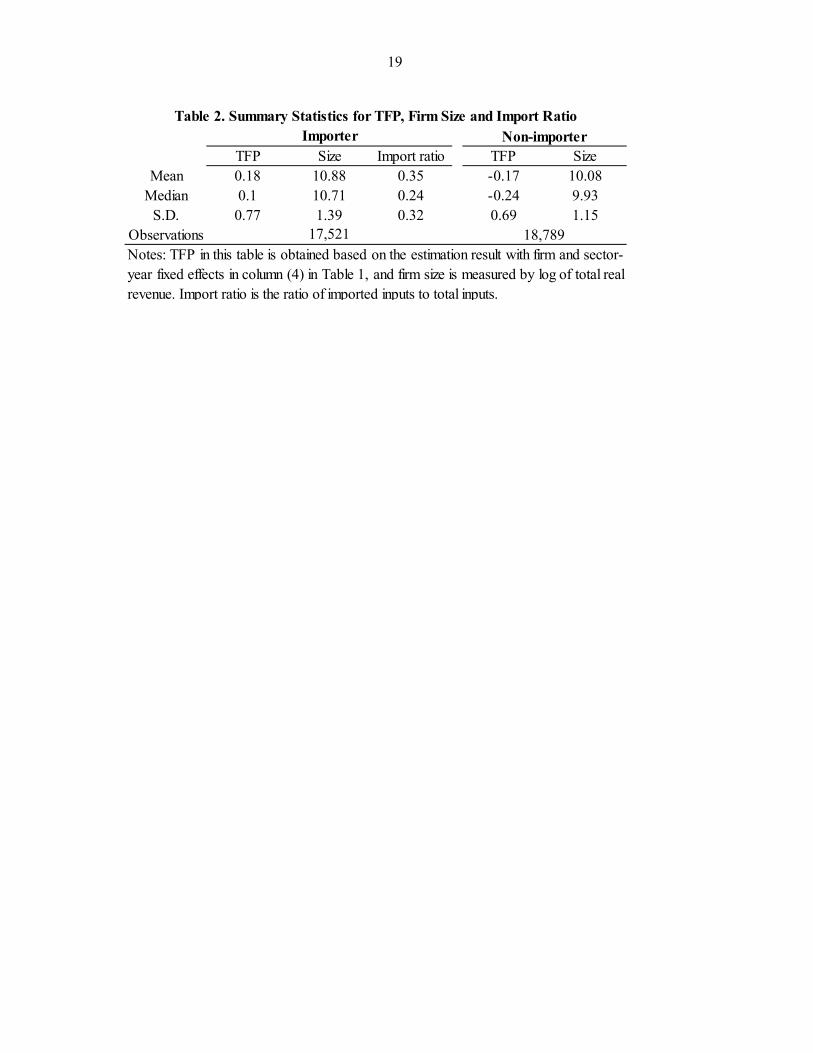
Our main data source is the Survey of Business Activities (SBA) from the Statistics Korea (KOSTAT). This annual survey data covers all firms with 50 or more employees and 300 million won or greater capital from 2006 to 2012. We limit our sample to the manufacturing sector classified into 22 industry categories.11 The data includes firm-level information on revenue, employment, inputs, capital, investment, imports, etc. To convert the nominal values into real terms, each variable is deflated with relevant price indexes. Revenue is deflated with the sector-level Producer Price Index (PPI) compiled by the Bank of Korea. Capital and investment are deflated with the domestic PPI for capital goods. Total inputs are divided into domestic and imported inputs and deflated by the sector-level effective PPI and Imported Inputs Price Index, respectively, which are constructed in a similar way to those in Amiti and Konings (2007).12 Import ratio is calculated using these real terms of imported and total inputs. The data is unbalanced panel including 36,310 observations of 8,232 firms. Table 2 presents the summary statistics of TFP estimated based on OLS and firm size measured by log of total real revenue.13 It shows that importing firms tend to be larger in size and more productive than non-importing firms, which is also confirmed in Figure 3, and that importers import one third of their input materials on average.14 According to Table 3-a, the number of importers continuously increases until 2009 but decreases in 2010 while the import ratio decreases in 2009 and recovers in 2010. This pattern partly suggests that firms reduce their import intensity temporarily due to the negative impact of the Global Financial Crisis, and many small importing firms who suffered more than larger firms finally choose not to import or to

11 The industry classification in the SBA follows the Korean Standard Industry Classification (KSIC), and the manufacturing sector includes 24 two-digit KSIC code industries from 10 to 33. Among them, the following two industries are excluded from our sample due to the following reasons: Importing firms are not observed in Manufacture of Tobacco Products (12); matching with price data is problematic and the share of importing firms is very low in Printing and Reproduction of Recorded Media (18).

12 We use the sector-level Import Price Index and Producer Price Index combined with the bilateral sector-level Input-Output table in 2005 to construct the sector-level imported and domestic input price index for 13 manufacturing industries classified by IO table. That is, the effective domestic Producer Price Index is constructed as an average PPI weighted by domestic input share, while the effective Import Price Index is constructed as an average IPI weighted by imported input share. Then, 13 industries based on the IO classification are finally matched with 22 KSIC code industries in our sample. See Ahn, Park, and Park (2015) for more details on this procedure.

13 TFP estimation results from OLS are provided in Table 1.

14 According to Table 3-b, firms that imported continuously throughout the sample period since their entry are more likely to have larger output level, number of employees, and capital with a high import ratio about 0.4 on average compared to those firms that never imported and switched their import status.

6

exit in the following year, resulting in a more skewed importing to larger firms as well as the pro-cyclical average import ratio. However, this summary statistics do not identify what mechanism makes the use of imported inputs actually affect productivity. Moreover, the TFP based on OLS estimate is vulnerable to potential biases including simultaneity bias with input decisions, not to mention that with import decisions. Therefore, we proceed with a model and estimation strategy in the next section to discuss more specifically how the import ratio affects firms’ TFP and how the effect changed over the business cycle.

III. MODEL AND EMPIRICAL STRATEGY

In this section, we discuss our empirical strategy for TFP estimation. We consider production of a firm i at time t as a Cobb-Douglas function of capital, labor, and intermediate inputs:

(1) The dependent variable is output measured as log of total real revenue; l is labor input measured as log of the number of employees; k is capital represented by log of total real tangible assets; m is log of real intermediate inputs; and is TFP level in log.15 As in Kasahara and Rodrigue (2008) and Halpern et al. (2011, 2015), we explicitly assume the contribution of imports to productivity, thereby breaking down the TFP term into one from the use of imported inputs (i.e., ) and the other from all else (i.e., ), where f is a ratio of imported inputs to total input purchase. Our focus is not simply on how much input a firm imports itself but on the share of imported inputs relative to total input materials because the underlying mechanism that imported inputs enhance productivity is based on either higher quality of imported inputs relative to domestic ones or imperfect substitution between foreign and domestic input varieties as discussed in Halpern et al. (2015).

A typical challenge in estimating the production function parameters with OLS is that a simultaneity bias caused by the correlation between unobservable productivity shocks and the firm’s input choices and a sample selection bias resulted from the relationship between the unobservable productivity shocks and the firm’s liquidation decision yield inconsistent estimates.16 To address these endogeneity problems, we closely follow Kasahara and Rodrigue (2008) and Halpern et al. (2015) that explicitly take into account the role of importing in applying the Olley-Pakes (O-P) methodology.17 Specifically, Olley-Pakes (1996) define a firm’s investment demand as an increasing function of two state variables, capital and productivity shocks, which allow the inversed investment function to be used as a proxy for unobservable productivity in the production function so that the O-P estimation yields 15 Please refer to Kasahara and Rodrigue (2008) and Halper et al. (2011, 2015) for more details on theoretical foundation. We employ their theory in the model section and focus more on the empirical part in which our main contribution is.

16 In a nutshell, if a positive productivity shock leads firms to use more inputs causing a positive correlation between regressors and the error term, OLS estimates will be upwardly biased. Also, if a firm’s exit decision depends on its productivity, the sample will be selected based on the unobservable productivity shocks causing a selection bias in the estimates.

17 Please refer to appendix for details of Olley-Pakes methodology.

7

consistent estimates for the production function parameters by applying the semiparametric regression techniques. Kasahara and Rodrigue (2008) and Halpern et al. (2011) add the import intensity as another state variable based on the idea that the decision on how much inputs to import should be made by firms one period earlier just as the investment decision for the current period is made in the previous period. Thus, the productivity is expressed as a function of investment, capital, and import ratio, and we employ this methodology in our estimation to find out the role of imported inputs in production. Using the production function estimates, the log of measured TFP of firm i at time t can be expressed as the following equation of the difference between actual output and the model’s prediction:

(2) Once the log valued TFP is converted into level value18, we can perform various sets of accounting exercises to understand fluctuations in aggregate productivity in detail. Noting that the aggregate TFP is obtained as the sum of the firm-level TFP weighted by output share, the aggregate TFP is decomposed into two parts: unweighted average TFP and the covariance between output share and TFP as shown in the following equation:

∑ ∙

∑

(3)

where ∑

denotes firm i’s output share, and the upper bar denotes the average value

across firms in a given year t. The covariance term can be interpreted as measuring the efficient resource allocation across firms. The higher the covariance term is, the higher output share goes to a firm with higher TFP (e.g., Olley and Pakes, 1996; Pavcnik, 2002).

As shown in equation (4), the growth of aggregate TFP can thus be expressed as the sum of the change in simple industry-level average TFP and the one in covariance term. The change in covariance term is further broken down into two parts; one is an intra-firm efficiency associated with the pure change in TFP level in each firm keeping its output share unchanged and the other is an inter-firm efficiency associated with resource reallocation across firms putting a larger weight on output share growth for firms with higher TFP.19 Intuitively, this covariance term decomposition suggests that the efficiency of resource allocation can be enhanced by improving TFP in a firm with more resources (intra-firm efficiency) or allocating more resources to more productive firms (inter-firm efficiency).20

18 From this point on, denotes TFP in level.

19 Decomposition of the covariance term into intra- and inter-firm efficiency includes entrants and exiting firms as well as continuers since our data is unbalanced panel. Specifically, apart from the unconditional average term, an exit effect is included in the intra-firm efficiency term, while an entry effect is reflected in the inter-firm efficiency term because 0 and 0 for entrants and 0 and 0 for exiting firms, thereby corresponding to an alternative expression in previous studies (e.g., Baily et al., 1992; Bartelsman, and Doms, 2000; Foster, Haltiwanger, and Krizan, 2001).

20 This is similar to the shift-share approach widely used in the structural change literature (e.g., McMillan et al. 2014).

8

∆ ∆ ∆∑ (4) ∆

∑ ∙ ∆

∑ ∆ ∙

Given the focus of the paper, it is important to note that one can always separate out the part of TFP due to imported inputs by plugging instead of in equations above. This will basically guide us to evaluate the role of imports in aggregate TFP dynamics in general, and, in particular, how much the collapse in imports affected aggregate TFP during the Global Financial Crisis (GFC) period as well as to what extent the skewed nature of the distribution of importers amplified the shocks.

IV. RESULTS

A. Production Function Estimation with O-P Methodology

Table 4 presents the estimation results for equation (1) from the OLS, Within-group, and O-P estimators. Column (1) shows the OLS estimation result, and the coefficients of import ratio as well as labor, capital, and materials are estimated to be positive and statistically significant. However, due to simultaneity and sample selection issues discussed in the previous section, the OLS estimator is likely to yield biased estimates. Specifically, variables that are more responsive to a contemporary productivity shock—such as labor—tend to be upwardly biased due to the positive correlation between input choices and productivity shocks. On the other hand, firms with larger capital are less likely to exit even under negative productivity shocks, causing sample selection and hence, downwardly biased estimates for the coefficient of capital. Columns (2) through (4) report results from the Within-group estimators with firm or/and sector-year fixed effects, and the coefficient for import ratio is estimated to be positive and statistically significant but with smaller magnitude than in column (1). With firm fixed effects, estimates in column (3) and (4) control for the simultaneity between inputs and firm-specific time-invariant shocks, and with sector-year fixed effects, estimates in column (2) and (4) control for the correlation between inputs and sector-year specific shocks. However, these within-estimators still cannot address the simultaneity between input choices and within-firm shocks varying over time. The O-P estimation result that controls for both simultaneity and selection bias is presented in column (5). As discussed above, we can confirm that estimates from OLS and within estimators tend to be overestimated for labor coefficients and underestimated for capital coefficients compared to O-P estimates. The coefficient for import ratio from the O-P estimation is significantly positive and larger than its OLS estimate. The difference between OLS and O-P estimates for import ratio can be partly attributed to sample selection, but also according to previous studies (Levinson and Petrin (2003), Kasahara and Rodrigue (2008)), the OLS estimates for import variables could be downwardly biased when the use of imported inputs is less responsive to a shock than other inputs even though the import

9

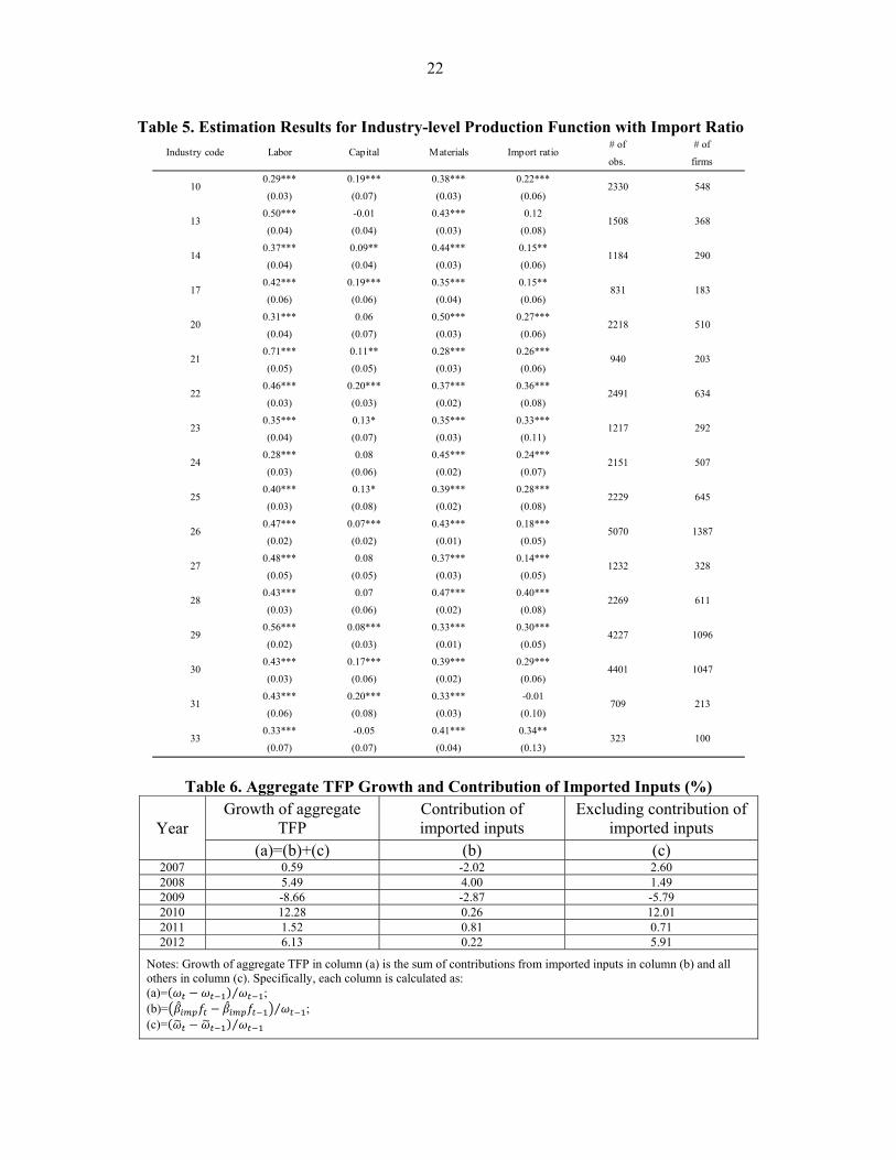
variable is positively correlated with productivity shocks. Overall, the O-P estimation result supports that an increase in import intensity has a significantly positive effect on output.21 Noting that Table 4 unveils the aggregate production function estimation result, assuming that all the input coefficients are identical across industries, we postulate that the contribution of each input may differ across industries due to industry-specific technological characteristics. Accordingly, we also present industry-specific O-P estimation results for 16 industries with more than 100 firms that have enough observations for reliable estimation results in Table 5. In most of the industries, the production function estimation result exhibits a positive and significant coefficient for import ratio, and the magnitude varies between 0.14 and 0.36. This result once again confirms that the share of imported inputs has a substantial impact on output across industries. Overall, production function estimation results imply that the use of imported inputs is an economically significant source of TFP, the part of the output level which is not explained by labor, capital, and materials. Given that the extent to which the use of imported inputs affects TFP varies across industries, a relevant question to ask is whether its importance as a source of TFP remains valid at the aggregate-level, which is the main subject of the next section.

B. Aggregate-level TFP Accounting

Using the industry-level O-P estimation result reported in Table 5, we obtain the measured TFP as the difference between a firm’s actual output and the predicted value using labor, capital and materials. Then, we aggregate the measured TFP weighted by each firm’s output share and calculate its growth. In the aggregate TFP growth, we separate a part associated with imported inputs and the remaining part to investigate how much import ratio contributed to the TFP growth. In Table 6, the aggregate TFP growth is indicated in column (a), and the contribution of imported inputs and other factors are separately reported in column (b) and (c). In the sample period between 2006 and 2012, TFP of the manufacturing sector has grown except for the Global Financial Crisis from 2008 to 2009 during which TFP declined by 8.7 percent (column (a)). As shown in column (b), 2.9 percent of the decrease is attributed to the shrinkage of import intensity which accounts for about one third of the drop. Overall, the change in the relative use of imported inputs appears to have significant impacts on the pattern of aggregate TFP growth across years. Given the non-negligible role of imported inputs on the aggregate-level TFP growth, we turn to the TFP growth caused by firm-level import decisions and delve into the channel through

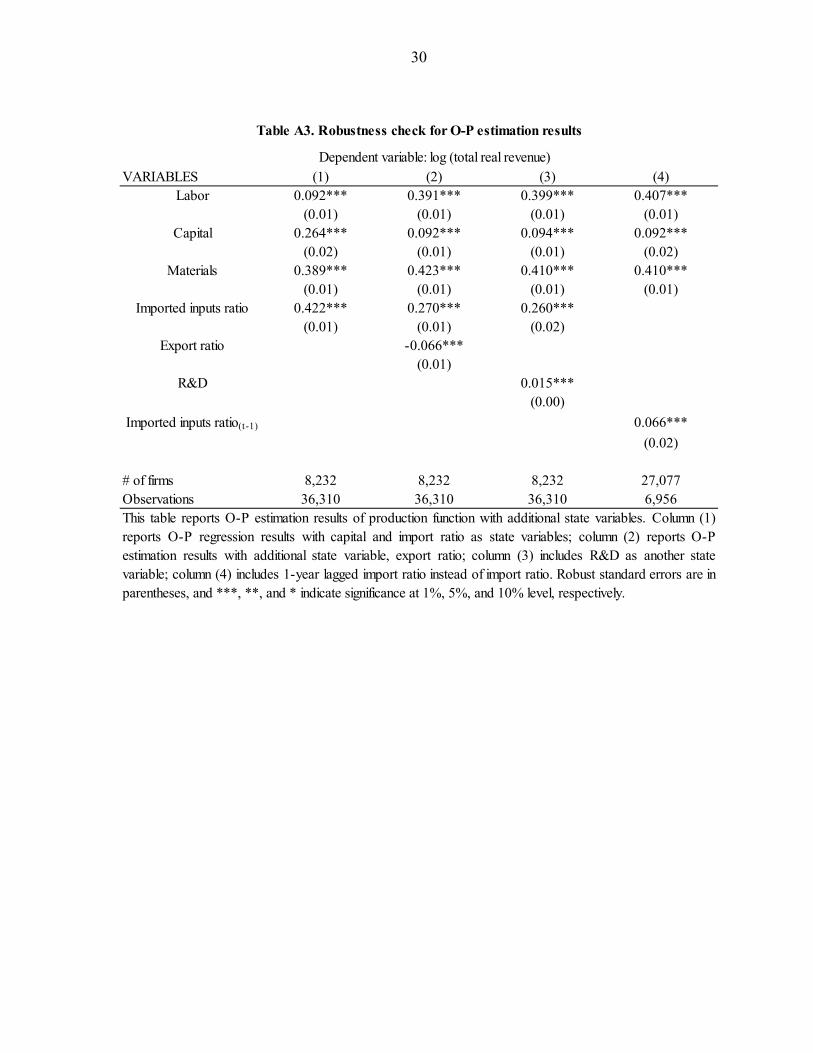
21 Table A3 presents O-P estimation results with additional explanatory variables to check the robustness of our benchmark O-P estimation model. We add other state variables such as export ratio and R&D in the model to consider the additional factor that could affect the productivity. In column (2) and (3), the results show that import ratio still has a positive and significant coefficient even after controlling the effects of export ratio and R&D. In column (4), we also include a 1-year lagged import ration variable replacing the import ratio, and the result shows that import ratio also has a positive dynamic effect that affects the productivity in the next period with smaller magnitude than the current period of import ratio does. The sample size with lagged import ratio, however, is more limited than the benchmark model.

10

which the import affects the aggregate TFP growth. As presented in equation (3), the growth of aggregate TFP can be decomposed into simple average TFP growth across firms and a covariance term between firm-level output share and TFP growth. We simply replace total

TFP ( ) with TFP due to imported inputs ( ) in equations (3) and (4). As shown in Table 7, the growth of aggregate TFP explained by imported inputs varies across years and dropped dramatically from 2008 to 2009 by 31 percent (column (a)). This large drop can be decomposed into simple average and a covariance term. Among the TFP growth due to import ratio (-31 percent), the part explained by the unweighted average growth of TFP is 1 percent (column (b)) and the remaining -32 percent is attributed to the covariance term (column (c)). This overwhelmingly large role of covariance term indicates that the aggregate-level TFP drop due to the import was not simply driven by an across-the-board decline in the use of imported inputs, but rather related to the efficiency losses from output share reallocation by the use of imported inputs which can occur either because a decline in the relative use of imported inputs was concentrated on firms with larger output share or because the market share shifted from firms with a large share of imported inputs to those with a small share of imported inputs or non-importers. The former will be captured by the intra-firm efficiency term while the latter is captured by the inter-firm efficiency term in a further decomposition as equation (4), which is reported in columns (d) and (e) respectively. In 2009, the contribution of intra-firm efficiency is measured at -39 percent while that of inter-firm efficiency is measured at 7 percent. This result means that the efficiency decrease mainly occurred due to the intra-firm efficiency loss through the decrease of imports by relatively larger firms while the inter-firm efficiency somewhat increased, suggesting that firms with higher TFP related to import ratio gained more output share in the market. Overall, the finding reveals that the decrease of imports by larger firms induced the huge drop in import-related TFP during the GFC, and the negative impact was magnified as the import activities are highly skewed to larger firms in Korea.

C. Industry-level TFP Accounting

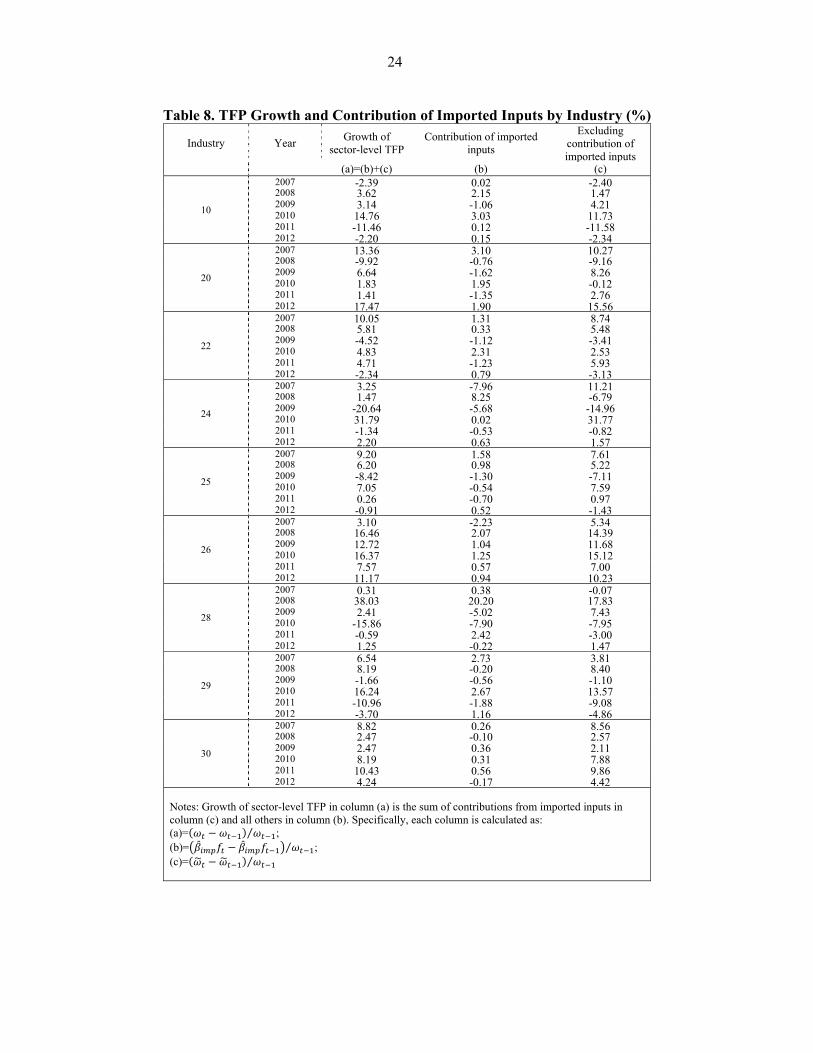
In this section, we repeat the above exercise at the industry level and report the industry-level TFP growth for selected industries to see variation across industries. For industry-level TFP, we report results for nine selected industries with more than 500 firms. We obtain the industry-level TFP and its annual growth using the production function estimation results by industry. As presented in Table 8, the contribution of imported inputs to TFP growth varies across industries, and the TFP growth resulting from changes in import intensity also differs across industries. Industries 22 (Rubber and Plastic Products), 24 (Basic Metal Products), 25 (Fabricated Metal Products, Except Machinery and Furniture), and 29 (Other Machinery and Equipment) had a sharp TFP drop ranging from approximately 2 percent to 21 percent in 2009, and the contribution of import ratio to the TFP drop ranged from about 0.6 percent to 6 percent. Industries 10 (Food Products), 20 (Chemicals and chemical products except pharmaceuticals, medicinal chemicals) and 28 (Electrical equipment) experienced a TFP decrease due to import ratio even though their aggregate TFP increased. Particularly, Industry 28

11

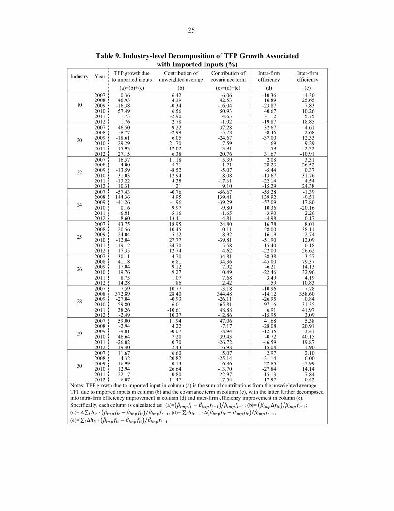
(Electrical equipment) also experienced a 16 percent drop in TFP in the following year, and the half of the drop is attributed to import ratio. This Industry-level result on the contribution of import ratio to TFP growth once again confirms that most industries suffered from the TFP reduction due to the import ratio during the GFC. We further decomposed the industry-level TFP growth explained by import intensity into simple average and an efficiency term. As shown in Table 9, the industry-level decomposition also maintains the similar patterns to those shown in the aggregate-level. Most of the selected industries with more than 500 firms suffered from a negative growth of TFP due to import ratio in 2009, ranging from -9 percent to -41 percent, and the decrease is mainly generated by a decrease in efficiency, which is a covariance between output share and productivity related to import ratio. The large contribution of covariance term suggests that the productivity drop is more amplified as import activities are more concentrated to larger firms. Also, a further decomposition of the covariance term into intra- and inter-firm efficiency unveils that the efficiency drop is mostly caused by a decrease in intra-firm efficiency rather than that in inter-firm efficiency, meaning that the loss of within-firm TFP due to decline of import ratio of relatively larger firms is greater than the TFP changes due to output share reallocation across firms. This covariance decomposition again supports that the negative effect of the reduction in imported inputs on TFP during the GFC is also intensified at the industry-level since firms with larger output share are more skewed to import activities. To get a clearer idea on the respective role of each item in accounting decompositions reported above, we document industry-level regression results in Table 10 and Table 11. In Table 10, we regress each of columns (b) and (c) on column (a) in Table 8 to understand how much of the variation in industry-level TFP growth is explained by TFP due to imported inputs and other factors on average. By the property of accounting identity, sum of the coefficients across each regression should be always 1. Columns (1) and (3) indicate that TFP due to imported inputs explains, on average, about 20 percent of variation in TFP growth across sectors over time, while all other terms account for 80 percent of variation. Columns (2) and (4) further reveal that such a pattern did not change during the period when there were rapid drop and subsequent rebound in TFP growth. Table 11 repeats the accounting regression exercise with items in Table 9. We regress each of columns (b), (c), (d), and (e) on column (a) in Table 9, which gives an answer on how much of the variation in industry-level TFP growth due to imported inputs is explained by the growth in unweighted average TFP due to imported inputs and covariance term on average, with the latter further decomposed into intra- and inter-firm efficiency improvement. Again by the property of accounting identity, sum of coefficients in columns (1) and (3) or (2) and (4) should be always 1, while sum of coefficients in columns (5) and (7) or (6) and (8) should be equal to coefficients in columns (3) or (4). Accordingly, columns (1) and (3) show that covariance term tends to explain around 87 percent of variation in TFP growth due to imported inputs, and such a pattern did not change during the GFC and the subsequent recovery. More interestingly, columns (5)-(8) show that intra- and inter-firm efficiency improvement tend to explain equal portions of variation in changes in covariance term on average over the sample period, but during the turbulent period, most of the fluctuations in

12

covariance term stem from intra-firm efficiency improvement, corroborating the pattern described from aggregate-level accounting decomposition in Table 7.

V. CONCLUSION

Using the Korean manufacturing firm-level data, this paper confirms that three stylized facts on importing hold in Korea: the ratio of imported inputs in total inputs tends to be pro-cyclical, the use of imported inputs increases productivity, and larger firms are more likely to use imported inputs. Based on these three well-documented characteristics of imports, the paper assesses the extent to which imports contribute to the pro-cyclicality of productivity and finds that firm-level import decisions explain a non-trivial fraction of aggregate productivity fluctuations in Korea over the period between 2006 and 2012. Main findings of this paper suggest a possible link between the recent global productivity slowdown and global trade slowdown, which will be an interesting topic for future research.

13

REFERENCES

Aghion, Philippe, and Peter Howitt, 1992, “A Model of Growth through Creative Destruction.” Econometrica, Vol. 60, No. 2, pp. 323–51.

Ahn, JaeBin, Mary Amiti, and David Weinstein, 2011, “Trade Finance and the Great Trade

Collapse,” American Economic Review, Vol. 101, No. 3, pp. 298–302. Ahn, JaeBin, Chang-Gui Park, and Chanho Park, 2016, “Pass-through of Imported Input

Price to Domestic Producer Prices: Evidence from Sector-Level Data,” IMF Working Paper 16/23 (Washington: International Monetary Fund).

Amiti, Mary, Oleg Itskhoki, and Jozef Konings, 2014, “Importers, Exporters, and Exchange

Rate Disconnect,” American Economic Review, Vol. 104, No. 7, pp. 1942–78. Amiti, Mary, and Jozef Konings, 2007, “Trade Liberalization, Intermediate Inputs, and

Productivity: Evidence from Indonesia,” American Economic Review, Vol. 97, No. 5, pp. 1611–38.

Antràs, Pol, Teresa Fort, and Felix Tintelnot, 2014, “The Margins of Global Sourcing:

Theory and Evidence from U.S. Firms,” (unpublished; Cambridge, Massachusetts: Harvard University).

Baily, Martin N., Charles Hulten, David Campbell, Timothy Bresnahan, and Richard E.

Caves, 1992, “Productivity Dynamics in Manufacturing Plants,” Brookings Papers on Economic Activity: Microeconomics, Brookings Institution, pp. 187–267.

Bartelsman, Eric J., and Mark Doms, 2000, “Understanding Productivity: Lessons from

Longitudinal Microdata,” Journal of Economic Literature, Vol. 38, No. 3, pp. 569–94. Basu, Susanto, and John Fernald, 2001, “Why Is Productivity Procyclical? Why Do We

Care?” in New Developments in Productivity Analysis, Studies in Income and Wealth, Vol. 63, ed. by C. R. Hulten, E. R. Dean, and M. J. Harper, pp. 225–302 (Chicago: University of Chicago Press).

Bernard, Andrew, Bradford Jensen, and Peter Schott, 2009, “Importers, Exporters, and

Multinationals: A Portrait of Firms in the U.S. that Trade Goods,” in Producer dynamics: New Evidence from Micro Data, ed. By T. Dunne, J. B. Jensen, and M. J. Roberts, 513–52 (Chicago: University of Chicago Press).

Constantinescu, Cristina, Aaditya Mattoo, and Michele Ruta, 2015, “The Global Trade

Slowdown: Cyclical or Structural?” IMF Working Paper No. 15/6 (Washington: International Monetary Fund).

De Long, J. B., and Waldmann, R. J., 1997, “Interpreting Procyclical Productivity: Evidence

from a Cross-Nation Cross-Industry Panel,” Economic Review-Federal Reserve Bank of San Francisco, (1), pp. 33–52.

14

Eichengreen, Barry, Donghyun Park, and Kwanho Shin, 2015, “The Global Productivity Slump: Common and Country-Specific Factors,” NBER Working Paper No. 21556 (Cambridge, Massachusetts: National Bureau of Economic Research).

Engel, C., and Wang, J, 2011, “International Trade in Durable Goods: Understanding

Volatility, Cyclicality, and Elasticities,” Journal of International Economics, Vol. 83, No. 1, pp. 37–52.

Ethier, W. J., 1982, “National and International Returns to Scale in the Modern Theory of

International Trade,” American Economic Review, Vol. 72, No. 3, pp. 389–405. Feenstra, Robert C., James R. Markusen, and William Zeile, 1992, “Accounting for Growth

with New Inputs: Theory and Evidence,” American Economic Review, Vol. 82, No. 2, pp. 415–21.

Field, Alexander J., 2010, “The Procyclical Behavior of Total Factor Productivity in the

United States, 1890-2004,” Journal of Economic History, Vol. 70, No. 2, pp. 326–50. Foster, Lucia, John Haltiwanger, and Cornell Krizan. 2001. “Aggregate Productivity Growth.

Lessons from Microeconomic Evidence.” In New Developments in Productivity Analysis, ed. Charles R. Hulten, Edwin R. Dean, and Michael J. Harper, 303-372. Chicago: University of Chicago Press.

Goldberg, Pinelopi K., Amit K. Khandelwal, Nina Pavcnik, and Petia Topalova, 2010,

“Imported Intermediate Inputs and Domestic Product Growth: Evidence from India,” Quarterly Journal of Economics, Vol. 125, No. 44, pp. 1727–67.

Gopinath, Gita, and Brent Neiman, 2014, “Trade Adjustment and Productivity in Large

Crises,” American Economic Review, Vol. 104, No. 3, pp. 793–831. Grossman, G. M., and E. Helpman, 1991, “Quality Ladders in the Theory of Growth,”

Review of Economic Studies, Vol. 58, No. 1, pp. 43–61. Halpern, Laszlo, Miklos Koren, and Adam Szeidl, 2011, “Imported Inputs and Productivity,”

CeFiG Working Papers No.8. Halpern, Laszlo, Miklos Koren, and Adam Szeidl, 2015, “Imported Inputs and Productivity,”

American Economic Review, Vol. 105, No. 12, pp. 3660–3703. Kasahara, Hiroyuki, and Beverly Lapham, 2013, “Productivity and the Decision to Import

and Export: Theory and Evidence,” Journal of International Economics, Vol. 89, No. 2, pp. 297–316.

Kasahara, Hiroyuki, and Joel Rodrigue, 2008, “Does the Use of Imported Intermediates

Increase Productivity? Plant-Level Evidence,” Journal of Development Economics, Vol. 87, No. 1, pp. 106–18.

Kim, Sangho, Hyunjoon Lim, and Donghyun Park, 2009, “Imports, Exports and Total Factor

Productivity in Korea,” Applied Economics, Vol. 41, No. 14, pp. 1819–34.

15

Lawrence, Robert Z., and David E. Weinstein, 1999, “Trade and Growth: Import-Led or Export-Led? Evidence from Japan and Korea,” NBER Working Paper No. 7264 (Cambridge, Massachusetts: National Bureau of Economic Research).

Levinsohn, James, and Amil Petrin, 2003, “Estimating Production Functions using Inputs to

Control for Unobservables,” Review of Economic Studies, Vol. 70, No. 2, pp. 317–41. McMillan, Magaret, Dani Rodrik, and Íñigo Verduzco-Gallo, 2014, “Globalization,

Structural Change, and Productivity Growth, with an Update on Africa,” World Development, 63: 11–32.

Manova, Kalina, and Zhiwei Zhang, 2009, “China's Exporters and Importers: Firms,

Products, and Trade Partners,” NBER Working Paper No. 15249 (Cambridge, Massachusetts: National Bureau of Economic Research).

Muendler, Marc-Andreas, 2004, “Trade, Technology and Productivity: A Study of Brazilian

Manufacturers 1986-1998,” Center for Economic Studies and Ifo Institute Working Paper 1148.

Obstfeld, Maurice, and Kenneth Rogoff, 2000, “The Six Major Puzzles in International

Macroeconomics: Is There a Common Cause?” In NBER Macroeconomics Annual 2000, 15: 339–412. MA: MIT Press.

Olley, G. Steven, and Ariel Pakes, 1996, “The Dynamics of Productivity in the

Telecommunications Equipment Industry,” Econometrica, Vol. 64, No. 6, pp. 1263–97. Pakes, Arie, 1994, “Dynamic Structural Models, Problems and Prospects Part II: Mixed

Continuous- Discrete Control Problems, and Market Interactions,” in Advances in Econometrics: Sixth World Congress, Vol.2, ed. by Christopher Sims, 171–259 (Cambridge: Cambridge University Press).

Pavcnik, Nina, 2002, “Trade Liberalization, Exit, and Productivity Improvements: Evidence

from Chilean Plants,” Review of Economic Studies, Vol. 69, No. 1, pp. 245–76. Romer, P. M., 1990, “Endogenous Technological Change,” Journal of Political Economy,

Vol. 98, S71–S102. Sbordone, Argia M., 1997, “Interpreting the Procyclical Productivity of Manufacturing

Sectors: External Effects or Labor Hoarding?” Journal of Money, Credit and Banking, Vol. 29, No. 11, pp. 26–45.

Topalova, Petia, and Amit Khandelwal, 2011, “Trade Liberalization and Firm Productivity:

The Case of India,” Review of Economics and Statistics, Vol. 93, No. 3, pp. 995–1009. Van Biesebroeck, Johannes, 2003, “Productivity Dynamics with Technology Choice: An

Application to Automobile Assembly,” Review of Economic Studies, Vol. 70, No. 1, pp. 167–98.

16

17

Figure 3. Distribution of TFP and Firm Size (Importer vs. Non-Importer)

Notes: TFP in this figure is obtained based on the estimation result with firm and sector-year fixed effects in column (4) in Table 1, and firm size is measured by log of total real revenue.

0.2

.4.6

Ke

rne

l De

nsi

ty

-4 -2 0 2 4TFP_fsyfe

Importer

Non-importer

kernel = epanechnikov, bandwidth = 0.0962

TFP distribution (Importer vs. Non-importer)

0.1

.2.3

.4K

ern

el D

en

sity

5 10 15 20ln_Output

Importer

Non-importer

kernel = epanechnikov, bandwidth = 0.1662

Firm Size distribution (Importer vs. Non-importer)

18

VARIABLES(1) (2) (3) (4)

Labor 0.467*** 0.499*** 0.414*** 0.410***-0.006 -0.006 -0.021 -0.018

Capital 0.171*** 0.157*** 0.165*** 0.095***-0.004 -0.004 -0.014 -0.008

Materials 0.431*** 0.413*** 0.146*** 0.139***-0.005 -0.005 -0.012 -0.01

Constant 2.500*** 2.512*** 5.613*** 6.205***-0.022 -0.031 -0.198 -0.151

Sector-Year FE N Y N YFirm FE N N Y YObservations 36,310 36,310 36,310 36,310R-squared 0.864 0.88 0.966 0.973

Table 1. OLS Estimation Results for Production FunctionDependent variable: log (total real revenue)

Note: This table reports OLS regression results of production function. Column (1) reportsOLS regression results with no fixed effects; column (2) reports estimates with sector-year fixed effects; column (3) includes firm fixed effects; column (4) includes both sector-year and firmfixed effects. Robust standard errors are in parentheses, and ***, **, and * indicatesignificance at 1%, 5%, and 10% level, respectively.

19

TFP Size Import ratio TFP SizeMean 0.18 10.88 0.35 -0.17 10.08

Median 0.1 10.71 0.24 -0.24 9.93S.D. 0.77 1.39 0.32 0.69 1.15

ObservationsNotes: TFP in this table is obtained based on the estimation result with firm and sector-year fixed effects in column (4) in Table 1, and firm size is measured by log of total realrevenue. Import ratio is the ratio of imported inputs to total inputs.

Table 2. Summary Statistics for TFP, Firm Size and Import RatioImporter Non-importer

17,521 18,789

20

Observations TFP Size Import ratio Observations TFP Size2006 2,309 0.134 10.71 0.35 3,300 -0.175 10.112007 2,560 0.153 10.83 0.34 3,023 -0.191 10.152008 2,577 0.191 10.93 0.34 2,859 -0.187 10.22009 2,786 0.201 10.95 0.31 2,391 -0.186 10.192010 2,302 0.223 11.16 0.36 1,968 -0.141 10.412011 2,421 0.199 11.17 0.36 2,558 -0.15 10.472012 2,566 0.166 11.11 0.38 2,690 -0.141 10.49

Table 3a. Average TFP and Firm Size (Importer vs. Non-importer)Non-importerImporter

Notes: This table reports the number of firms, average TFP, the size of importers and non-importers andthe import ratio of importers for each year. TFP is obtained from firm and sector-year fixed effectsestimation reported in column (4) in Table 1. The size indicates log value of total real revenue.

Output Labor Capital Materials Import ratio No. of firms Observations10.61 4.93 9.3 9.78 0.17-1.3 -0.86 -1.48 -1.64 -0.28

11.11 5.23 9.72 10.42 0.39-1.55 -1.09 -1.71 -1.75 -0.329.99 4.57 8.78 9.07-0.99 -0.57 -1.23 -1.4510.7 4.98 9.36 9.86 0.16-1.22 -0.82 -1.43 -1.56 -0.2810.79 5.03 9.47 9.96 0.18-1.3 -0.88 -1.46 -1.63 -0.29

10.06 4.62 8.74 9.22 0.13-1.15 -0.72 -1.4 -1.53 -0.26

Notes: This table reports summary statistics by firms’ importing and/or surviving status with standarddeviations are in parentheses. Importers are firms that continuously imported foreign intermediates in thesample, and Non-importers are firms that never imported foreign intermediates in the sample. Switchersare firms that switched their import status in the sample. Survivors are firms that did not exit during thesample period (2006-2012) whereas Quitters exit during the sample period. Output is logarithm of realrevenue, Labor is logarithm of number of employees, Materials are logarithm of total inputs purchased,and Import ratio is the ratio of imported foreign inputs to total inputs.

Survivors 5,256 27,605

Quitters 2,976 8,705

Non-importers

- 2,743 8,480

Switchers 3,771 20,773

Table 3b. Descriptive Statistics by import/survival status

All firms 8,232 36,310

Importers 1,718 7,057

21

(1) (2) (3) (4) (5)OLS FE FE FE O-P

Labor 0.459*** 0.492*** 0.411*** 0.408*** 0.092***-0.006 -0.006 -0.021 -0.018 -0.013

Capital 0.170*** 0.155*** 0.163*** 0.095*** 0.264***-0.004 -0.004 -0.014 -0.008 -0.017

Materials 0.429*** 0.411*** 0.150*** 0.142*** 0.389***-0.005 -0.005 -0.012 -0.01 -0.009

Imported inputs ratio 0.233*** 0.217*** 0.100*** 0.075*** 0.422***-0.011 -0.011 -0.012 -0.01 -0.007

Sector-Year FE N Y N YFirm FE N N Y Y# of firms 8,232 8,232 8,232 8,232 8,232Observations 36,310 36,310 36,310 36,310 36,310R-squared 0.866 0.883 0.967 0.973

Table 4. Estimation Results for Production Function with Import Ratio

Dependent variable: log (total real revenue)

Notes: This table reports regression results of production function. Column (1) reports OLSregression results with no fixed effects; column (2) reports estimates with sector-year fixed effects;column (3) includes firm fixed effects; column (4) includes both sector-year and firm fixed effects;column (5) presents estimates from Olley-Pakes methodology. Robust standard errors are inparentheses, and ***, **, and * indicate significance at 1%, 5%, and 10% level, respectively.

22

Table 5. Estimation Results for Industry-level Production Function with Import Ratio

Table 6. Aggregate TFP Growth and Contribution of Imported Inputs (%)

Year Growth of aggregate

TFP Contribution of imported inputs

Excluding contribution of imported inputs

(a)=(b)+(c) (b) (c) 2007 0.59 -2.02 2.60 2008 5.49 4.00 1.49 2009 -8.66 -2.87 -5.79 2010 12.28 0.26 12.01 2011 1.52 0.81 0.71 2012 6.13 0.22 5.91

Notes: Growth of aggregate TFP in column (a) is the sum of contributions from imported inputs in column (b) and all others in column (c). Specifically, each column is calculated as: (a)= ⁄ ; (b)= ⁄ ; (c)= ⁄

# of # of

obs. firms

0.29*** 0.19*** 0.38*** 0.22***

(0.03) (0.07) (0.03) (0.06)

0.50*** -0.01 0.43*** 0.12

(0.04) (0.04) (0.03) (0.08)

0.37*** 0.09** 0.44*** 0.15**

(0.04) (0.04) (0.03) (0.06)

0.42*** 0.19*** 0.35*** 0.15**

(0.06) (0.06) (0.04) (0.06)

0.31*** 0.06 0.50*** 0.27***

(0.04) (0.07) (0.03) (0.06)

0.71*** 0.11** 0.28*** 0.26***

(0.05) (0.05) (0.03) (0.06)

0.46*** 0.20*** 0.37*** 0.36***

(0.03) (0.03) (0.02) (0.08)

0.35*** 0.13* 0.35*** 0.33***

(0.04) (0.07) (0.03) (0.11)

0.28*** 0.08 0.45*** 0.24***

(0.03) (0.06) (0.02) (0.07)

0.40*** 0.13* 0.39*** 0.28***

(0.03) (0.08) (0.02) (0.08)

0.47*** 0.07*** 0.43*** 0.18***

(0.02) (0.02) (0.01) (0.05)

0.48*** 0.08 0.37*** 0.14***

(0.05) (0.05) (0.03) (0.05)

0.43*** 0.07 0.47*** 0.40***

(0.03) (0.06) (0.02) (0.08)

0.56*** 0.08*** 0.33*** 0.30***

(0.02) (0.03) (0.01) (0.05)

0.43*** 0.17*** 0.39*** 0.29***

(0.03) (0.06) (0.02) (0.06)

0.43*** 0.20*** 0.33*** -0.01

(0.06) (0.08) (0.03) (0.10)

0.33*** -0.05 0.41*** 0.34**

(0.07) (0.07) (0.04) (0.13)

31 709 213

33 323 100

29 4227 1096

30 4401 1047

27 1232 328

28 2269 611

25 2229 645

26 5070 1387

23 1217 292

24 2151 507

21 940 203

22 2491 634

17 831 183

20 2218 510

2330 548

13 1508 368

14 1184 290

Industry code Labor Capital Materials Import ratio

10

23

Table 7. Decomposition of Aggregate TFP Growth associated with Imported Inputs (%)

Year TFP growth due

to imported inputs (a)=(b)+(c)

Contribution of Unweighted average

(b)

Contribution of covariance term

(c)=(d)+(e)

Intra-firm efficiency

(d)

Inter-firm efficiency

(e)

2007 -25.97 3.92 -29.88 -30.97 1.09 2008 69.93 3.38 66.55 60.78 5.77 2009 -31.11 1.09 -32.20 -39.31 7.10 2010 3.78 14.03 -10.25 -12.80 2.55 2011 12.57 -6.72 19.29 10.28 9.01 2012 3.10 4.94 -1.84 -10.16 8.32

Notes: TFP growth due to imported input in column (a) is the sum of contributions from the unweighted average TFP due to imported inputs in column (b) and the covariance term in column (c), with the latter further decomposed into intra-firm efficiency improvement in column (d) and inter-firm efficiency improvement in column (e). Specifically, each column is calculated as: (a)= ; (b)= ∆ ̅ ;

(c)=∆∑ ∙ ̅ ;

(d)=∑ ∙ ∆ ̅ ; (e)=∑ ∆ ∙ ̅

24

Table 8. TFP Growth and Contribution of Imported Inputs by Industry (%) Industry Year

Growth of sector-level TFP

Contribution of imported inputs

Excluding contribution of imported inputs

(a)=(b)+(c) (b) (c)

10

2007 -2.39 0.02 -2.40 2008 3.62 2.15 1.47 2009 3.14 -1.06 4.21 2010 14.76 3.03 11.73 2011 -11.46 0.12 -11.58 2012 -2.20 0.15 -2.34

20

2007 13.36 3.10 10.27 2008 -9.92 -0.76 -9.16 2009 6.64 -1.62 8.26 2010 1.83 1.95 -0.12 2011 1.41 -1.35 2.76 2012 17.47 1.90 15.56

22

2007 10.05 1.31 8.74 2008 5.81 0.33 5.48 2009 -4.52 -1.12 -3.41 2010 4.83 2.31 2.53 2011 4.71 -1.23 5.93 2012 -2.34 0.79 -3.13

24

2007 3.25 -7.96 11.21 2008 1.47 8.25 -6.79 2009 -20.64 -5.68 -14.96 2010 31.79 0.02 31.77 2011 -1.34 -0.53 -0.82 2012 2.20 0.63 1.57

25

2007 9.20 1.58 7.61 2008 6.20 0.98 5.22 2009 -8.42 -1.30 -7.11 2010 7.05 -0.54 7.59 2011 0.26 -0.70 0.97 2012 -0.91 0.52 -1.43

26

2007 3.10 -2.23 5.34 2008 16.46 2.07 14.39 2009 12.72 1.04 11.68 2010 16.37 1.25 15.12 2011 7.57 0.57 7.00 2012 11.17 0.94 10.23

28

2007 0.31 0.38 -0.07 2008 38.03 20.20 17.83 2009 2.41 -5.02 7.43 2010 -15.86 -7.90 -7.95 2011 -0.59 2.42 -3.00 2012 1.25 -0.22 1.47

29

2007 6.54 2.73 3.81 2008 8.19 -0.20 8.40 2009 -1.66 -0.56 -1.10 2010 16.24 2.67 13.57 2011 -10.96 -1.88 -9.08 2012 -3.70 1.16 -4.86

30

2007 8.82 0.26 8.56 2008 2.47 -0.10 2.57 2009 2.47 0.36 2.11 2010 8.19 0.31 7.88 2011 10.43 0.56 9.86 2012 4.24 -0.17 4.42

Notes: Growth of sector-level TFP in column (a) is the sum of contributions from imported inputs in column (c) and all others in column (b). Specifically, each column is calculated as: (a)= ⁄ ; (b)= ⁄ ; (c)= ⁄

25

Table 9. Industry-level Decomposition of TFP Growth Associated with Imported Inputs (%)

Industry Year TFP growth due

to imported inputs Contribution of

unweighted average Contribution of covariance term

Intra-firm efficiency

Inter-firm efficiency

(a)=(b)+(c) (b) (c)=(d)+(e) (d) (e)

10

2007 0.36 6.42 -6.06 -10.36 4.30 2008 46.93 4.39 42.53 16.89 25.65 2009 -16.38 -0.34 -16.04 -23.87 7.83 2010 57.49 6.56 50.93 40.67 10.26 2011 1.73 -2.90 4.63 -1.12 5.75 2012 1.76 2.78 -1.02 -19.87 18.85

20

2007 46.50 9.22 37.28 32.67 4.61 2008 -8.77 -2.99 -5.78 -8.46 2.68 2009 -18.61 6.05 -24.67 -37.00 12.33 2010 29.29 21.70 7.59 -1.69 9.29 2011 -15.93 -12.02 -3.91 -1.59 -2.32 2012 27.15 6.38 20.76 31.67 -10.91

22

2007 16.57 11.18 5.39 2.08 3.31 2008 4.00 5.71 -1.71 -28.23 26.52 2009 -13.59 -8.52 -5.07 -5.44 0.37 2010 31.03 12.94 18.08 -13.67 31.76 2011 -13.22 4.38 -17.61 -22.14 4.54 2012 10.31 1.21 9.10 -15.29 24.38

24

2007 -57.43 -0.76 -56.67 -55.28 -1.39 2008 144.36 4.95 139.41 139.92 -0.51 2009 -41.26 -1.96 -39.29 -57.09 17.80 2010 0.16 9.97 -9.80 10.36 -20.16 2011 -6.81 -5.16 -1.65 -3.90 2.26 2012 8.60 13.41 -4.81 -4.98 0.17

25

2007 43.75 18.95 24.80 16.78 8.01 2008 20.56 10.45 10.11 -28.00 38.11 2009 -24.04 -5.12 -18.92 -16.19 -2.74 2010 -12.04 27.77 -39.81 -51.90 12.09 2011 -19.12 -34.70 15.58 15.40 0.18 2012 17.35 12.74 4.62 -22.00 26.62

26

2007 -30.11 4.70 -34.81 -38.38 3.57 2008 41.18 6.81 34.36 -45.00 79.37 2009 17.04 9.12 7.92 -6.21 14.13 2010 19.76 9.27 10.49 -22.46 32.96 2011 8.75 1.07 7.68 3.49 4.19 2012 14.28 1.86 12.42 1.59 10.83

28

2007 7.59 10.77 -3.18 -10.96 7.78 2008 372.89 28.40 344.48 -14.12 358.60 2009 -27.04 -0.93 -26.11 -26.95 0.84 2010 -59.80 6.01 -65.81 -97.16 31.35 2011 38.26 -10.61 48.88 6.91 41.97 2012 -2.49 10.37 -12.86 -15.95 3.09

29

2007 59.00 11.94 47.06 41.68 5.38 2008 -2.94 4.22 -7.17 -28.08 20.91 2009 -9.01 -0.07 -8.94 -12.35 3.41 2010 46.64 7.20 39.43 -0.72 40.15 2011 -26.02 0.70 -26.72 -46.59 19.87 2012 19.40 2.43 16.98 15.08 1.90

30

2007 11.67 6.60 5.07 2.97 2.10 2008 -4.32 20.82 -25.14 -31.14 6.00 2009 16.99 0.13 16.86 22.85 -5.99 2010 12.94 26.64 -13.70 -27.84 14.14 2011 22.17 -0.80 22.97 15.13 7.84 2012 -6.07 11.47 -17.54 -17.97 0.42

Notes: TFP growth due to imported input in column (a) is the sum of contributions from the unweighted average TFP due to imported inputs in column (b) and the covariance term in column (c), with the latter further decomposed into intra-firm efficiency improvement in column (d) and inter-firm efficiency improvement in column (e). Specifically, each column is calculated as: (a)= ; (b)= ∆ ̅ ; (c)=∆∑ ∙ ̅ ; (d)= ∑ ∙ ∆ ̅ ;

(e)=∑ ∆ ∙ ̅

26

Table 10. Regression Results: Industry-level Decomposition of TFP Growth Associated with Imported Inputs

Dependent variable:

(1) (2) (3) (4)

(TFP growth)s t 0.195 *** 0.199 *** 0.805 *** 0.801 ***

(0.02) (0.02) (0.02) (0.00)

(TFP growth)s t × -0.021 0.021

(2009/2010 Dummy)t (0.06) (0.06)

Sector FE Yes Yes Yes Yes

Year FE Yes Yes Yes Yes

Obs 132 132 132 132

Adj R squared 0.669 0.644 0.967 0.967

Contribution of imported inputs Excluding contribution of imported inputs

Note: The dependent variable is contribution of imported inputs to TFP growth (columns (1)-(2)) or TFP growth excludingcontribution of imported inputs (columns (3)-(4)) in sector s in year t. Independent variable is TFP growth in sector s in year t.Columns (2) and (4) include additional independent variables, a dummy variable equal 1 for years 2009 and 2010 and 0 otherwise (notreported), and its interaction with TFP growth. Coefficients in columns (1) and (3) or columns (2) and (4) sum to 1. All columns include year and sector fixed effects. Robust standard errors are in parenthesis. Significance: * 10 percent; ** 5 percent; *** 1 percent.

27

Table 11. Regression Results: Industry-level Decomposition of TFP Growth associated with Imported Inputs

Dependent variable:

(1) (2) (3) (4) (5) (6) (7) (8)

(TFP growth due to imported inputs)s t 0.134 *** 0.118 0.866 *** 0.882 *** 0.455 *** 0.319 ** 0.411 *** 0.563 ***

(0.04) (0.05) (0.04) (0.05) (0.13) (0.13) (0.13) (0.13)

0.053 -0.053 0.435 ** -0.488 ***

(2009/2010 Dummy)t (0.08) (0.08) (0.18) (0.15)

Sector FE Yes Yes Yes Yes Yes Yes Yes Yes

Year FE Yes Yes Yes Yes Yes Yes Yes Yes

Obs 132 132 132 132 132 132 132 132

Adj R squared 0.339 0.342 0.899 0.9 0.502 0.557 0.586 0.655

Note: The dependent variable is contribution of unweighted averages to TFP growth due to imported inputs (columns (1)-(2)), contribution of covariance term to TFP growth due to imported inputs(columns (3)-(4)), intra-firm efficiency improvement (columns (5) and (6) or inter-firm efficiency improvement in sector s in year t. Independent variables is TFP growth due to imported inputs insector s in year t. Columns (2), (4), (6), and (8) include additional independent variables, a dummy variable equal 1 for years 2009 and 2010 and 0 otherwise (not reported), and its interaction withTFP growth due to imported inputs. Coefficients in columns (1) and (3) or columns (2) and (4) sum to 1, while coefficients in columns (5) and (7) or columns (5) and (8) sum to coefficients incolumns (3) or (4). All columns include year and sector fixed effects. Robust standard errors are in parenthesis. Significance: * 10 percent; ** 5 percent; *** 1 percent.

Contribution of unweighted average Contribution of covariance term Intra-firm efficiency Inter-firm efficiency

(TFP growth due to imported inputs)s t ×

28

Appendix

Table A1. Industry Classification (Korean Standard Industry Classification (KSIC)) Industry Code

Description

10 Food Products 11 Beverages 12 Tobacco Products 13 Textiles, Except Apparel 14 Wearing apparel, Clothing Accessories and Fur Articles 15 Tanning and Dressing of Leather , Luggage and Footwear 16 Wood Products of Wood and Cork ; Except Furniture 17 Pulp, Paper and Paper Products 18 Printing and Reproduction of Recorded Media 19 Coke, hard-coal and lignite fuel briquettes and Refined Petroleum Products

20 Chemicals and chemical products except pharmaceuticals, medicinal chemicals

21 Pharmaceuticals, Medicinal Chemicals and Botanical Products 22 Rubber and Plastic Products 23 Other Non-metallic Mineral Products 24 Basic Metal Products 25 Fabricated Metal Products, Except Machinery and Furniture

26 Electronic Components, Computer, Radio, Television and Communication Equipment and Apparatuses

27 Medical, Precision and Optical Instruments, Watches and Clocks 28 Electrical equipment 29 Other Machinery and Equipment 30 Motor Vehicles, Trailers and Semitrailers 31 Other Transport Equipment 32 Furniture 33 Other manufacturing

29

Table A2. Summary Statistics

Industry Data Summary Revenue Worker Capital Inputs Import

Ratio

Total Mean 10.61 4.93 9.30 9.78 0.17 S.D. 1.30 0.86 1.48 1.64 0.28 Obs. 36310 36310 36310 36310 36310

10 Mean 10.67 5.08 9.35 9.92 0.15 S.D. 1.36 0.95 1.45 1.64 0.28 Obs. 2330 2330 2330 2330 2330

11 Mean 11.31 5.38 10.42 10.36 0.15 S.D. 1.36 1.37 1.75 1.58 0.26 Obs. 186 186 186 186 186

13 Mean 9.93 4.64 8.86 8.91 0.19 S.D. 1.07 0.68 1.26 1.46 0.31 Obs. 1508 1508 1508 1508 1508

14 Mean 10.83 5.08 8.46 9.73 0.19 S.D. 1.23 0.81 1.79 1.54 0.31 Obs. 1184 1184 1184 1184 1184

15 Mean 10.79 4.88 8.48 9.87 0.31 S.D. 1.07 0.71 1.72 1.40 0.37 Obs. 271 271 271 271 271

16 Mean 10.78 4.86 9.87 10.10 0.23 S.D. 1.01 0.66 1.70 1.17 0.34 Obs. 126 126 126 126 126

17 Mean 10.83 4.85 9.85 10.15 0.20 S.D. 1.15 0.72 1.49 1.34 0.31 Obs. 831 831 831 831 831

19 Mean 13.06 5.65 11.26 12.43 0.35 S.D. 2.83 1.71 2.92 2.97 0.42 Obs. 77 77 77 77 77

20 Mean 11.22 5.02 9.94 10.52 0.26 S.D. 1.53 0.93 1.66 1.77 0.31 Obs. 2218 2218 2218 2218 2218

21 Mean 10.72 5.38 9.61 9.54 0.28 S.D. 1.16 0.86 1.37 1.43 0.31 Obs. 940 940 940 940 940

22 Mean 10.38 4.79 9.16 9.58 0.12 S.D. 1.08 0.76 1.16 1.39 0.25 Obs. 2491 2491 2491 2491 2491

23 Mean 10.59 4.90 9.61 9.61 0.17 S.D. 1.29 0.85 1.64 1.66 0.30 Obs. 1217 1217 1217 1217 1217

24 Mean 11.34 4.90 9.92 10.66 0.17 S.D. 1.37 0.87 1.56 1.78 0.29 Obs. 2151 2151 2151 2151 2151

25 Mean 10.39 4.73 9.12 9.47 0.11 S.D. 1.04 0.67 1.30 1.40 0.23 Obs. 2229 2229 2229 2229 2229

26 Mean 10.46 5.00 9.11 9.64 0.21 S.D. 1.38 0.95 1.53 1.76 0.30 Obs. 5070 5070 5070 5070 5070

27 Mean 9.98 4.75 8.73 9.03 0.23 S.D. 0.91 0.61 1.12 1.32 0.30 Obs. 1232 1232 1232 1232 1232

28 Mean 10.63 4.87 8.99 9.93 0.16 S.D. 1.21 0.78 1.35 1.48 0.27 Obs. 2269 2269 2269 2269 2269

29 Mean 10.38 4.8 9.09 9.49 0.14 S.D. 1.06 0.72 1.22 1.44 0.26 Obs. 4227 4227 4227 4227 4227

30 Mean 10.73 5.04 9.55 10.05 0.09 S.D. 1.24 0.91 1.25 1.49 0.21 Obs. 4401 4401 4401 4401 4401

31 Mean 11.11 5.29 10.11 9.88 0.15 S.D. 1.85 1.32 2.02 2.42 0.26 Obs. 709 709 709 709 709

32 Mean 10.64 4.83 9.09 9.88 0.11 S.D. 1.21 0.74 1.31 1.47 0.22 Obs. 320 320 320 320 320

33 Mean 10.00 4.65 8.44 9.12 0.28 S.D. 1.00 0.61 1.42 1.35 0.35 Obs. 323 323 323 323 323

30

VARIABLES (1) (2) (3) (4)Labor 0.092*** 0.391*** 0.399*** 0.407***

(0.01) (0.01) (0.01) (0.01)Capital 0.264*** 0.092*** 0.094*** 0.092***

(0.02) (0.01) (0.01) (0.02)Materials 0.389*** 0.423*** 0.410*** 0.410***

(0.01) (0.01) (0.01) (0.01)Imported inputs ratio 0.422*** 0.270*** 0.260***

(0.01) (0.01) (0.02)Export ratio -0.066***

(0.01)R&D 0.015***

(0.00)

Imported inputs ratio(t-1) 0.066***

(0.02)

# of firms 8,232 8,232 8,232 27,077Observations 36,310 36,310 36,310 6,956

Table A3. Robustness check for O-P estimation results

Dependent variable: log (total real revenue)

This table reports O-P estimation results of production function with additional state variables. Column (1)reports O-P regression results with capital and import ratio as state variables; column (2) reports O-Pestimation results with additional state variable, export ratio; column (3) includes R&D as another statevariable; column (4) includes 1-year lagged import ratio instead of import ratio. Robust standard errors are inparentheses, and ***, **, and * indicate significance at 1%, 5%, and 10% level, respectively.

31

Olley-Pakes Methodology

The Olley-Pakes methodology (Olley and Pakes(1996)) is based on the fact that the error term in a production function has two components; a white noise component, , and a time-varying productivity shock, . In estimating a production function, a typical problem is the correlation between unobserved productivity shocks, , and the inputs that are chosen by firms, which results in inconsistent OLS estimates. Also, there is an endogenous problem generated by sample selection because those firms with lower productivity than a certain threshold will exit the market, leading the surviving firms to have their productivity, , from a selected sample. Thus, this sample selection affected by the productivity shock will also have an effect on the input used. To address these issues, the Olley-Pakes methodology provides an approach based on firms’ dynamic optimization with an assumption that unobserved productivity, , follows a first-order Markov process and that capital is accumulated by dynamic investment process of firms. Through the profit maximization, firms’ investment demand function is generated and the investment demand depends on two state variables, capital and productivity such that , . The investment function is defined as monotonically increasing in productivity (Pakes(1994)), thus the function can be inverted and the productivity can be expressed as a function of capital and investment,

, . ,

Therefore, in estimating the production function, the first step is to estimate the consistent estimates of variable inputs except the state variable with an approximated function of capital and investment expressed as a polynomial approximation of them. The second step is to determine the probability of firms’ exit due to the productivity decrease below a certain threshold. The third step is to estimate the coefficient of the state variable using nonlinear least squares.