the role of structural mechanics in material design, control and optimization adnan ibrahimbegovic...
TRANSCRIPT
The role of structural mechanics in material design, control and optimization
Adnan Ibrahimbegovic
Ecole Normale Superieure / LMT-Cachan, Francee-mail : [email protected], fax : +33147402240
TU Gdansk, Poland, - December 8, 2003

LMT-Cachan : Laboratory of Mechanics and Technology
(Ecole Normale Sup / Univ. Pierre & Marie Curie / CNRS)
LMT-CachanIs located in Paris
Distance cca 3km : 30 min on foot 5 min by metro RER 2 – 60 min by car !
Introduction and motivation
LMT-Cachan is: - cca 150 researchers (with 45 Profs/Lecturers)- Center for experiments and measurements & Computer center
- 3 Divisions at LMT : • Div. « Material Science » (UPMC / J. Lemaitre) • Div. « Mechanical Eng. » (GM-ENS / P. Ladeveze) • Div. « Civil & Env. Eng. » (GC-ENS /A. Ibrahimbegovic)
-privileged environement for scientific research with: at least a couple of national or international meetings each year, seminar IDF / LMT, invited professors (for 1 month) …
LMT-Cachan : Laboratory of Mechanics and Technology(Ecole Normale Sup / Univ. Pierre & Marie Curie / CNRS
http://www.lmt.ens-cachan.fr

The role of structural mechanics in material
design, control and optimization
Outline :
• Part I: Micro-macro material modeling
• Part II: Structural optimization and control
Acknowledgements : D. Brancherie, D. Markovic, A. Delaplace, F. Gatuingt C. Knopf-Lenoir , P. Villon, UTC, France A. Kucerova, EU – Erasmus,
French Ministry of Research – ACI 2159

Micro-macro material modeling
Outline – part I •Introduction and motivation•Micro-macro modeling of inelastic behavior of structures• Discrete model ingredients• Time integration schemes for dynamic fracture analysis• Crack pattern analysis• Conclusions
Introduction and motivation
Reliable description of limit state behaviour of structures in their environment (multi-physics problems)
Final (worthy) goal
Available technologiesMacroscopic models (damage, plasticity, etc.) FE implementation (limit load, softening, etc.)
Goals of the present studyReliable interpretation of damage mechanisms
Representing local behaviour in heavily damaged areas (crack pattern, spacing, opening)
Flow comp. & crack propagation, dissipation cyclic loading, spalling
Proposed ApproachMicro-macro modeling with or without separation of scalesDiscrete models at micro- (and/or meso-) scale accounting for randomness of material microstructure
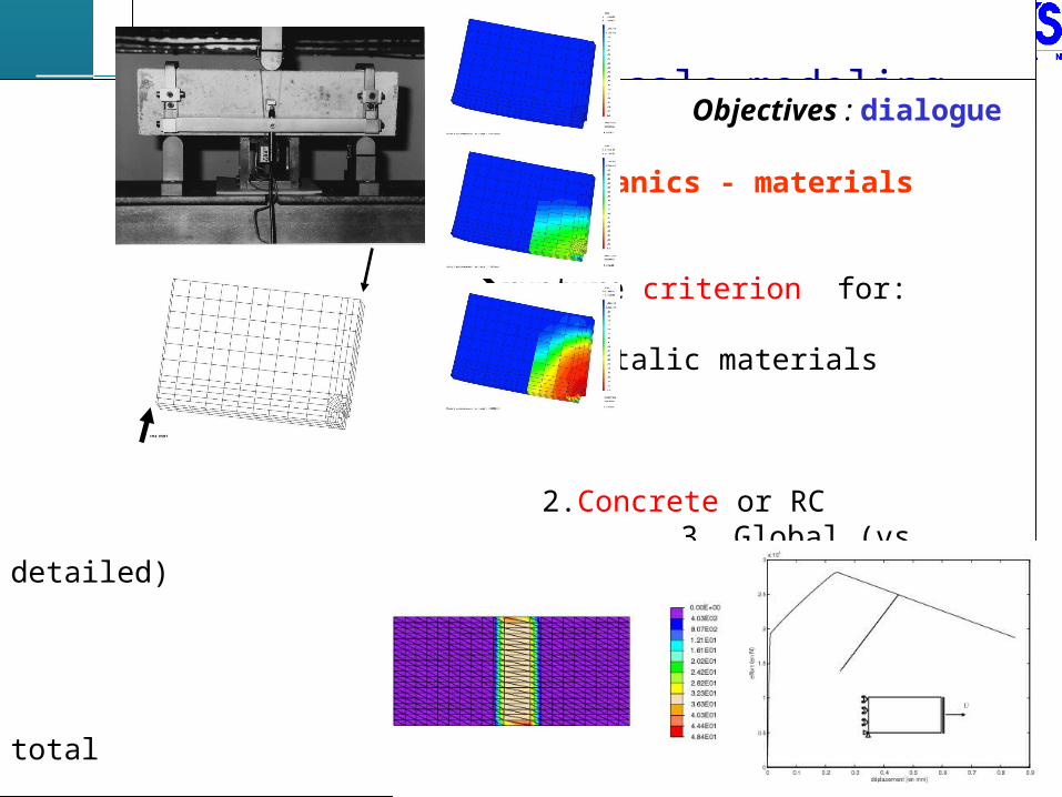
Multi-scale modeling
Objectives : dialogue mecanics - materials
rupture criterion for: 1.Metalic materials 2.Concrete or RC 3. Global (vs. detailed) analysis of damaged zone with a good estimate of total inelastic dissipation (no crack profiles) (difficulties w/r to multi-physics, coupling e.g. durability?),
A Ibrahimbegovic, D. Brancherie [2003] Comp. Mech. (M. Crisfield issue)

Multi-scale coupling : 3pt. - bending testi) FEM2 (Suquet et al. [1990])
ii) Strong coupling of scalesEach element “macro” repres. with a mesh of “micro” elementsA Ibrahimbegovic,D. Markovic [2003] CMAME (guest ed. P. Ladevèze)
Multiscale modeling : porous materials = 2phase
Remark : at “macro” scale we get a (novel) smeared model of coupled damage - plasticity A Ibrahimbegovic, D. Markovic, F.Gatuingt [2003] REEF Gurson/
contours show : macro-trace of stress tensor effective micro-plastic def.
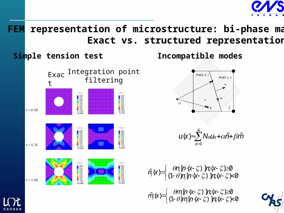
FEM representation of microstructure: bi-phase material Exact vs. structured representations
Simple tension test
Exact Integration pointfiltering
Incompatible modes
mnuNxua
aa ˆˆ)(4
1
0)()];([)1(
0)()];([)(ˆ
xnxnn
xnxnnxn
i
ii
0)()];([)1(
0)()];([)(ˆ
xnxnm
xnxnmxm
i
ii
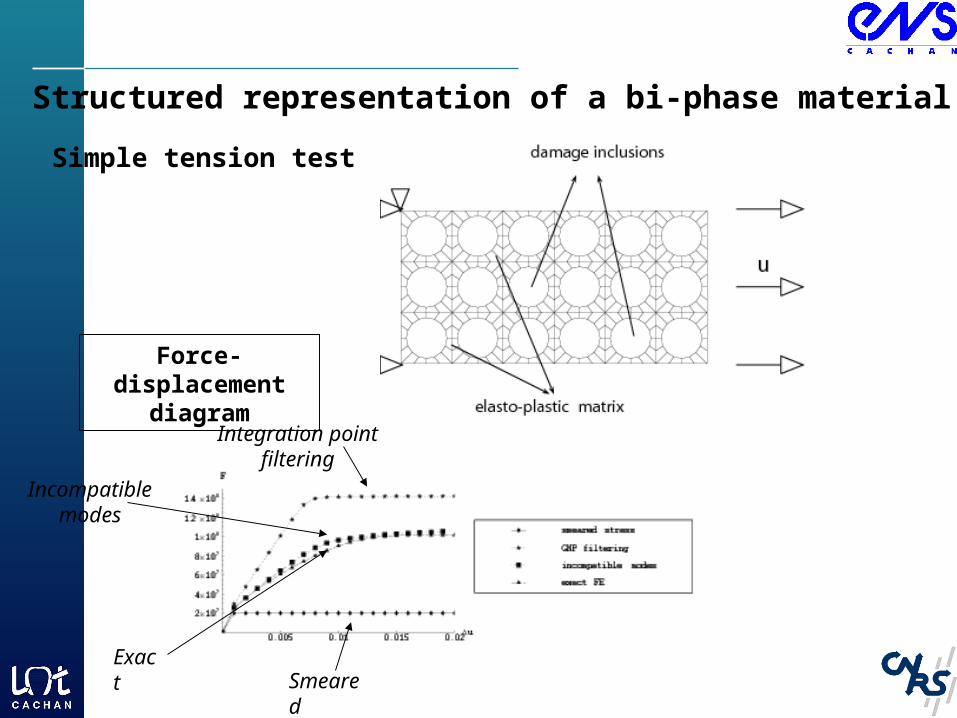
Structured representation of a bi-phase material
Simple tension test
Smeared
Integration pointfiltering
Incompatiblemodes
Exact
Force-displacement diagram
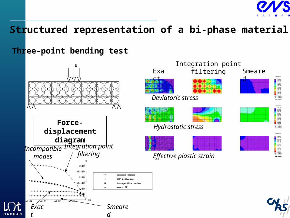
Structured representation of a bi-phase material
Three-point bending test
ExactIntegration point
filtering Smeared
Force-displacement diagram
SmearedExact
Integration pointfiltering
Incompatiblemodes
Deviatoric stress
Effective plastic strain
Hydrostatic stress
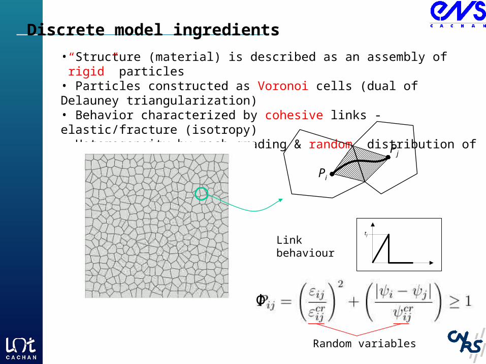
Discrete model ingredients
• Structure (material) is described as an assembly of ”rigid” particles• Particles constructed as Voronoi cells (dual of Delauney triangularization)• Behavior characterized by cohesive links - elastic/fracture (isotropy)• Heterogeneity by mesh grading & random distribution of fracture thresholds.
Pi
Pj
tf
Link behaviour
Random variables
Φ
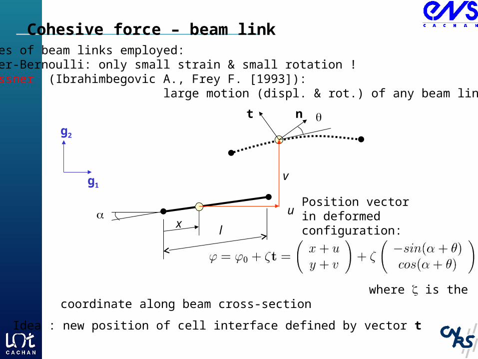
2 types of beam links employed:• Euler-Bernoulli: only small strain & small rotation !• Reissner (Ibrahimbegovic A., Frey F. [1993]): large motion (displ. & rot.) of any beam link
Cohesive force – beam link
lx
v
uPosition vector in deformed configuration:
g1
g2
nt
where is the coordinate along beam cross-section
Idea : new position of cell interface defined by vector t
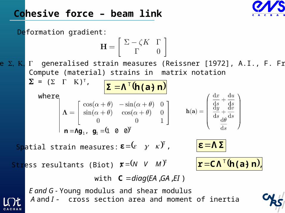
Compute (material) strains in matrix notation = ()T,
where nh(a)ΛΣ T
T11 001, gΛgn
Spatial strain measures: ,Tε ΣΛε
Stress resultants (Biot) : TMVNr ,T nh(a)CΛr
with ),,( EIGAEAdiagC
Deformation gradient:
where generalised strain measures (Reissner [1972], A.I., F. Frey [1993]).
E and G - Young modulus and shear modulus A and I - cross section area and moment of inertia
Cohesive force – beam link

Contact forces: two particles not linked with cohesive forces overlap at later stage. Penalization: contact force proportional to overlapping area (ij).
cohesion
contact
( U , F )
Contact forces

Numerical examples : microscale
Tension test –softening-likestress-strain diag.
Biaxial traction – crack pattern
FF
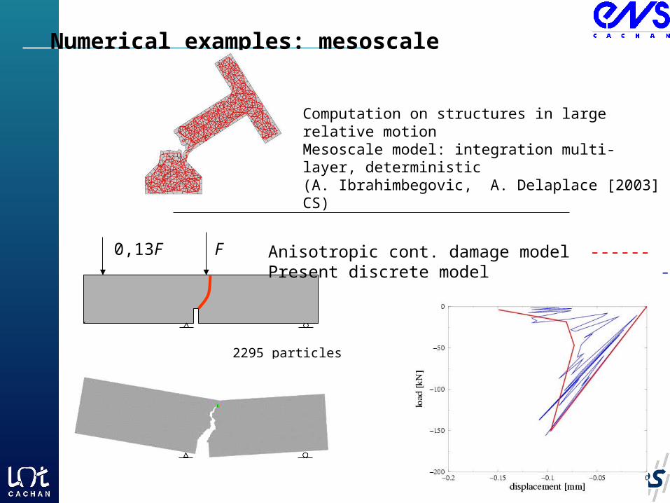
Numerical examples: mesoscale
Computation on structures in large relative motionMesoscale model: integration multi-layer, deterministic(A. Ibrahimbegovic, A. Delaplace [2003] CS)
0,13F F
2295 particles
Anisotropic cont. damage model ------Present discrete model ------
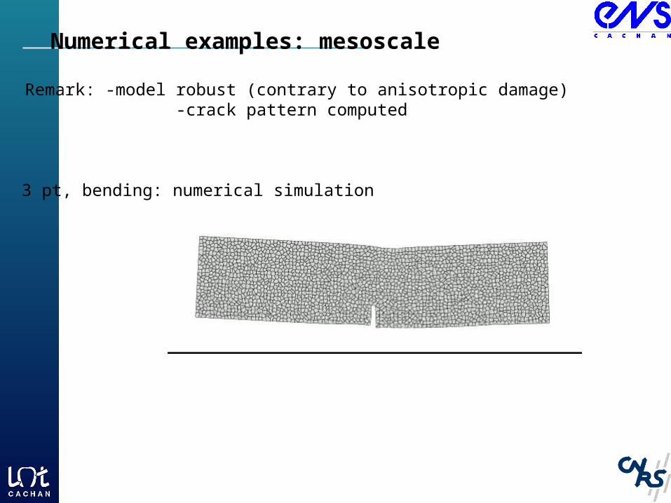
Numerical examples: mesoscale
Remark: -model robust (contrary to anisotropic damage) -crack pattern computed
3 pt, bending: numerical simulation

f
u
fc
Goal: damp undesirable high frequencies
Time integration schemes for dynamic fracture
Application: high rate loading
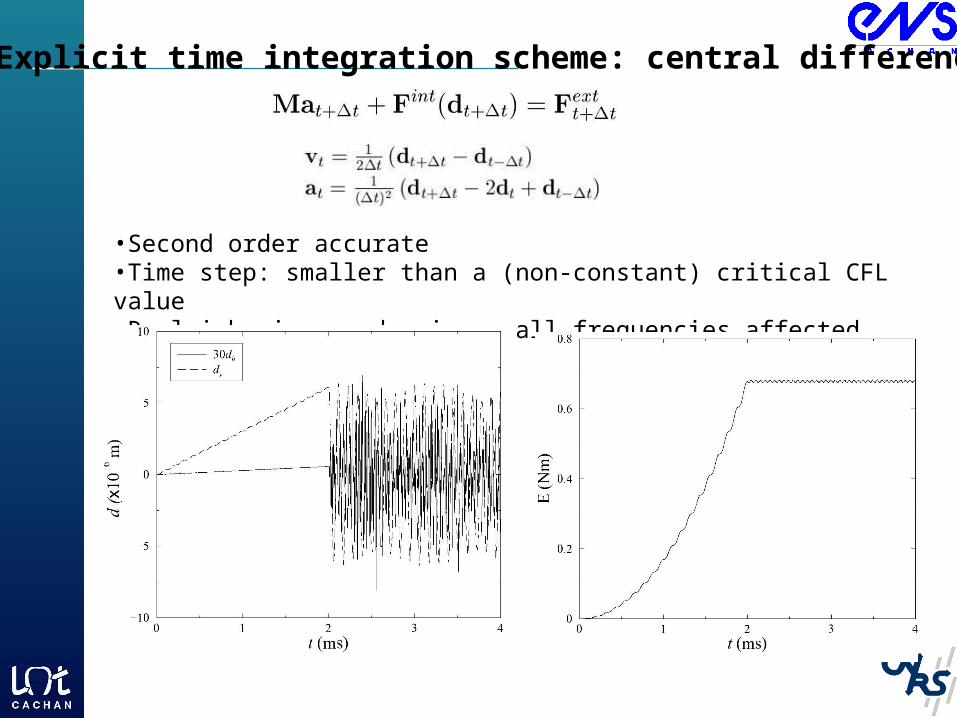
Explicit time integration scheme: central difference
•Second order accurate•Time step: smaller than a (non-constant) critical CFL value •Rayleigh viscous damping : all frequencies affected
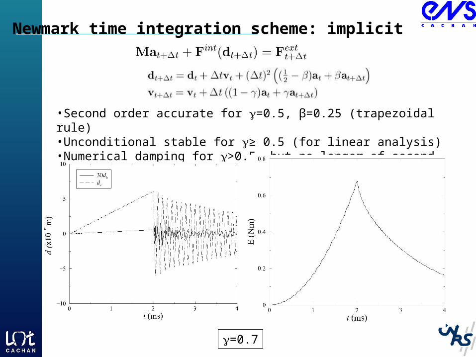
Newmark time integration scheme: implicit
•Second order accurate for =0.5, β=0.25 (trapezoidal rule) •Unconditional stable for ≥ 0.5 (for linear analysis)•Numerical damping for >0.5, but no longer of second order accuracy
=0.7
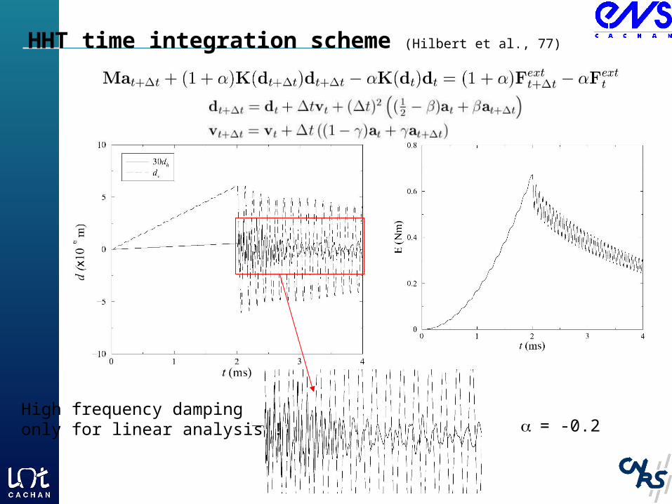
HHT time integration scheme (Hilbert et al., 77)
= -0.2High frequency dampingonly for linear analysis !
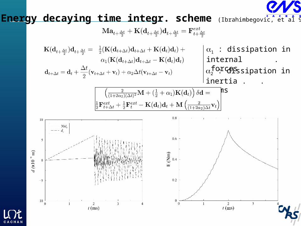
Energy decaying time integr. scheme (Ibrahimbegovic, et al 99. 02)
2 : dissipation in inertia . . terms
1 : dissipation in internal . forces
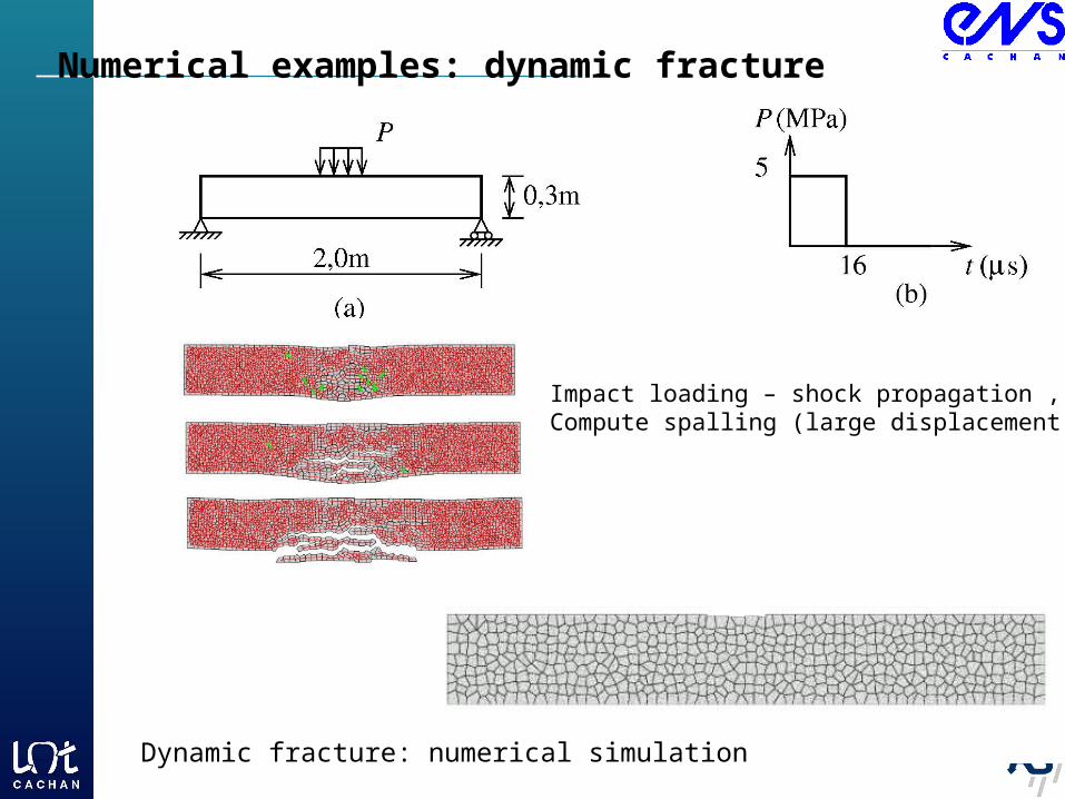
Impact loading – shock propagation , Compute spalling (large displacement!)
Numerical examples: dynamic fracture
Dynamic fracture: numerical simulation
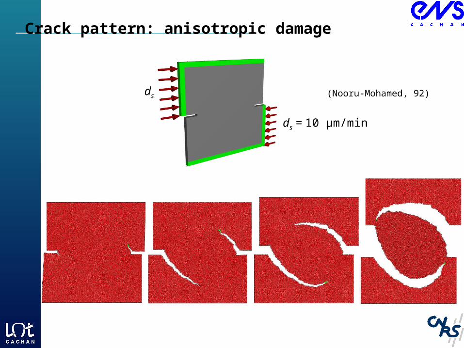
Crack pattern: anisotropic damage
ds = 10 µm/min
ds (Nooru-Mohamed, 92)
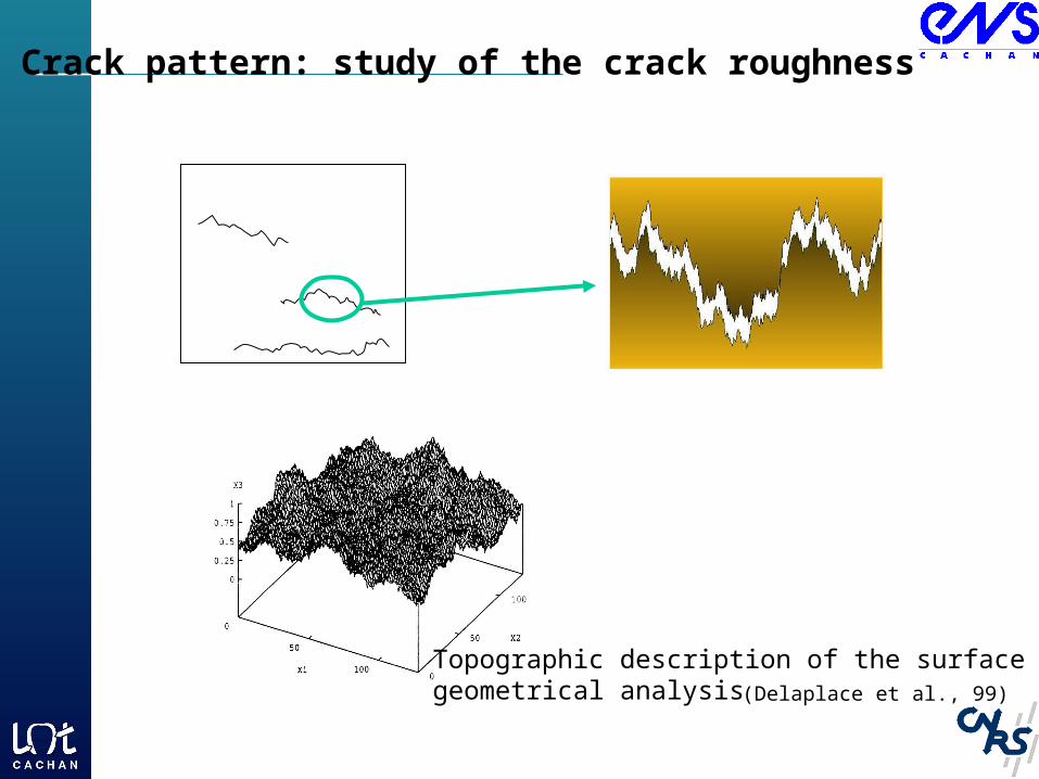
Crack pattern: study of the crack roughness
Topographic description of the surface area,geometrical analysis (Delaplace et al., 99)
~ 0,6 ± 0,2
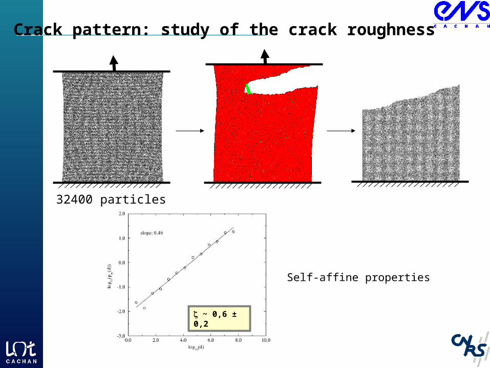
Crack pattern: study of the crack roughness
Self-affine properties
32400 particles
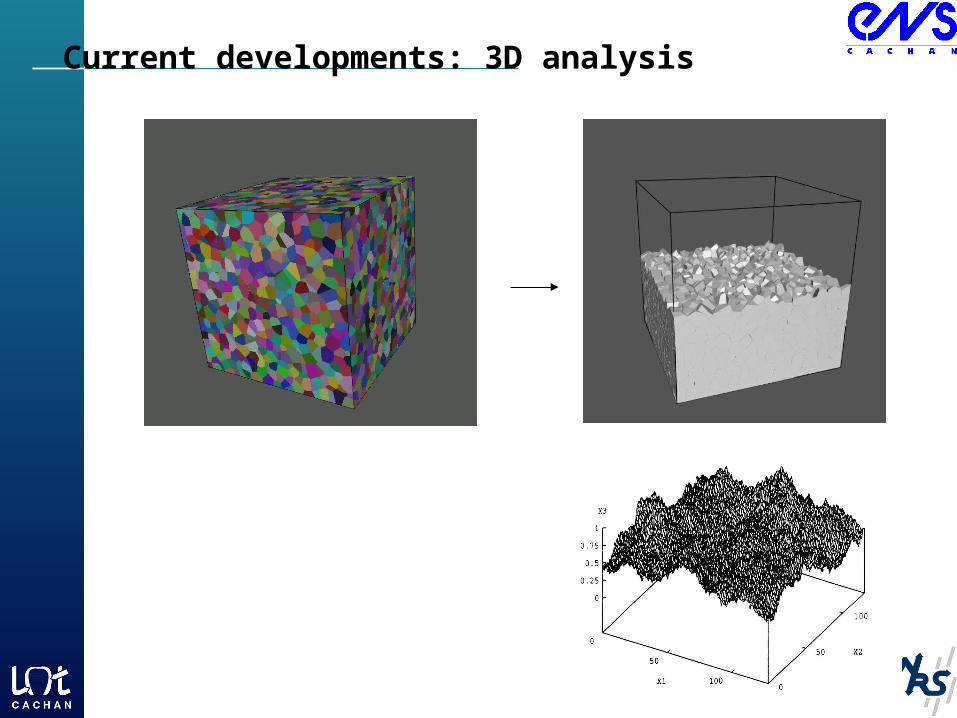
Current developments: 3D analysis

Conclusions – part I
•Multi-scale strongly coupled model of inelastic behavior with structured FE representation of microstructure •Discrete models – structural mechanics based modelling of fracture behaviour of heterogeneous materials . with brittle fracture at low or high rate loading. • Representation of local behaviour & Inelastic dissip. in damaged zone . (crack spacing, crack opening and crack propagation) + Post-processing - high accuracy description of cracked area . (Delaplace et al., 01)
•Capabilities beyond traditional cont. mech. models : e.g. spalling Essential role played by large diplacement/rotation structural theory!
Optimal control and optimal design of structures undergoing large rotations:
Acknowledgements : C. Knopf-Lenoir , P. Villon, UTC, France A. Kucerova, EU – Erasmus, French Ministry of Research,
Outline – part II :-Introduction and motivation-Problem model in nonlinear structural mechanics : 3D beam- Optimization : coupled mechanics-optimization problem- Solution procedures for coupled problem:-Conclusions
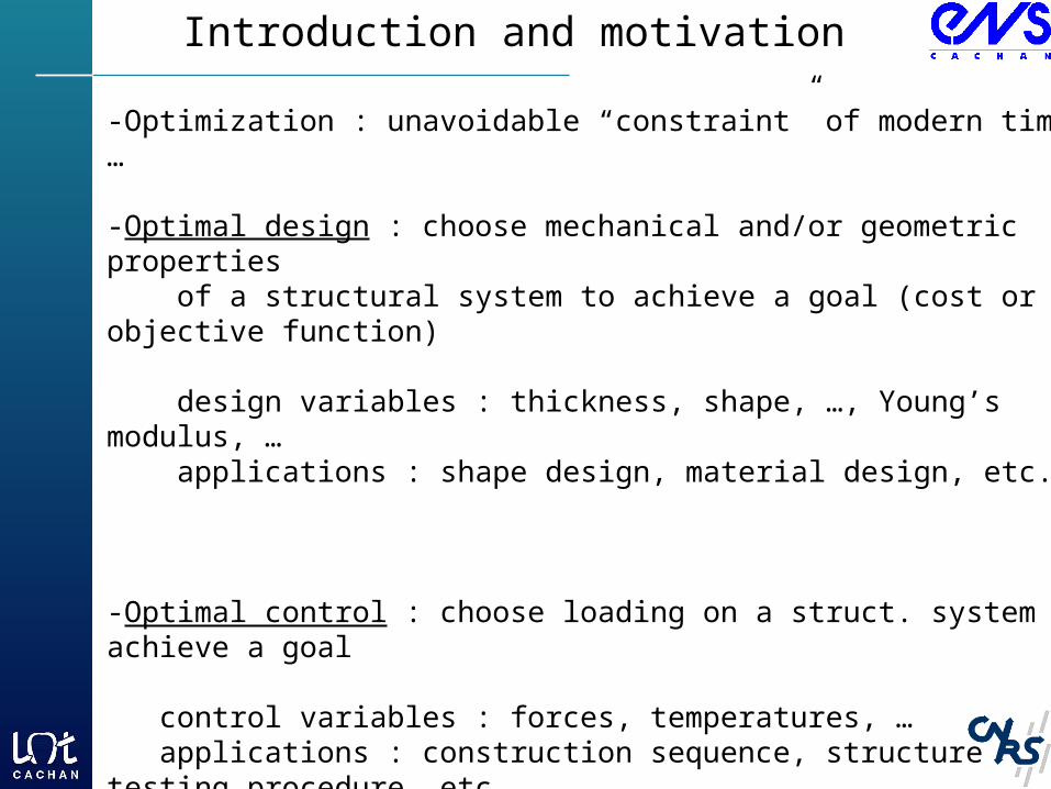
Introduction and motivation
-Optimization : unavoidable “constraint” of modern times …
-Optimal design : choose mechanical and/or geometric properties of a structural system to achieve a goal (cost or objective function) design variables : thickness, shape, …, Young’s modulus, … applications : shape design, material design, etc.
-Optimal control : choose loading on a struct. system to achieve a goal
control variables : forces, temperatures, … applications : construction sequence, structure testing procedure, etc.
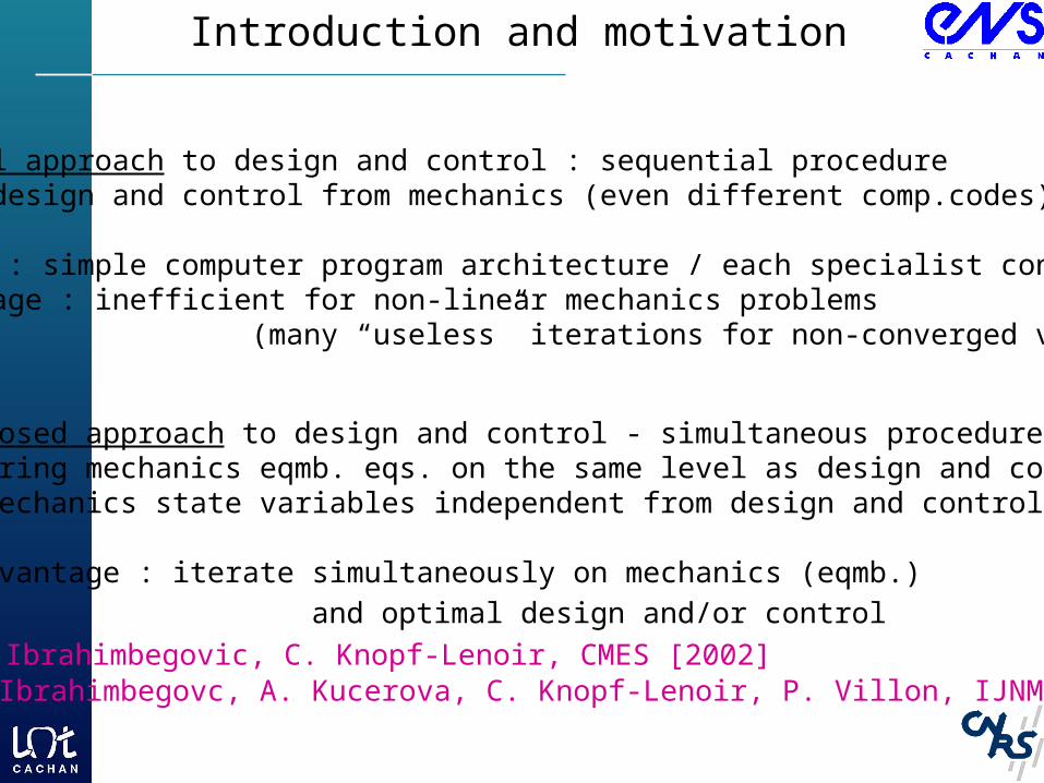
Introduction and motivation
-Traditional approach to design and control : sequential procedure separate design and control from mechanics (even different comp.codes)
-advantage : simple computer program architecture / each specialist contrib. -disadvantage : inefficient for non-linear mechanics problems (many “useless” iterations for non-converged value of opt.)
-Proposed approach to design and control - simultaneous procedure: bring mechanics eqmb. eqs. on the same level as design and control mechanics state variables independent from design and control variables
-advantage : iterate simultaneously on mechanics (eqmb.)
and optimal design and/or control A. Ibrahimbegovic, C. Knopf-Lenoir, CMES [2002] A. Ibrahimbegovc, A. Kucerova, C. Knopf-Lenoir, P. Villon, IJNME [2003]
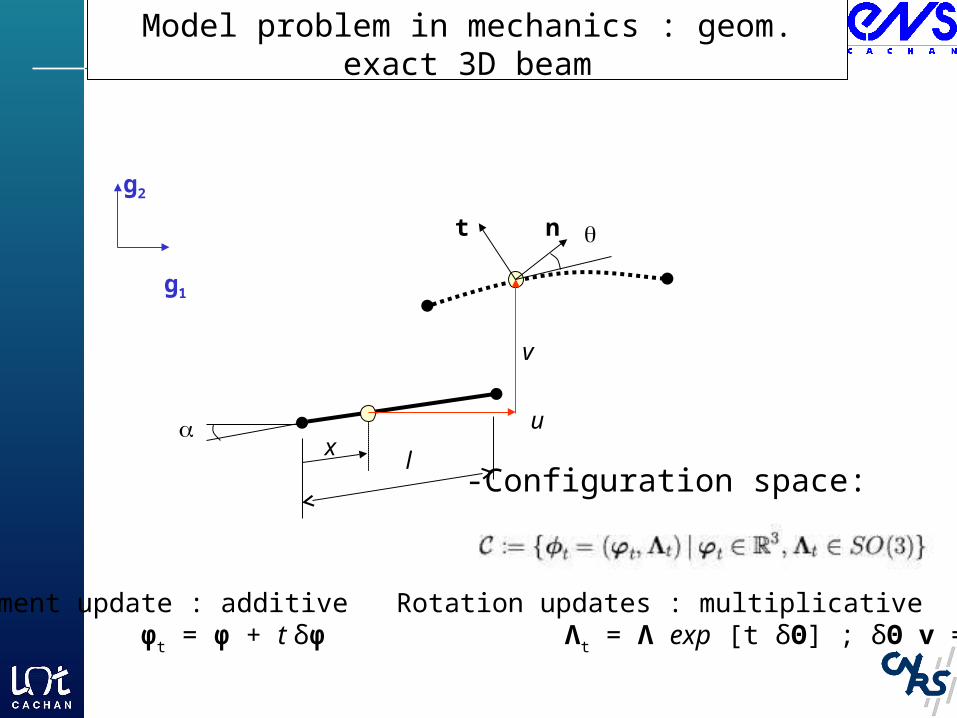
Model problem in mechanics : geom. exact 3D beam
-Configuration space:l
x
v
u
g1
nt
g2
Displacement update : additive Rotation updates : multiplicative φt = φ + t δφ Λt = Λ exp [t δΘ] ; δΘ v = δθ × v
Model problem in mechanics : geom. exact 3D beam
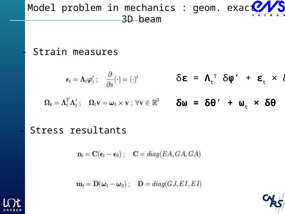
- Strain measures
- Stress resultants
δε = ΛtT δφ’ + εt × δθ
δω = δθ’ + ωt × δθ

Model problem in mechanics : geom. exact 3D beam
-Variational formulation : min. potential energy principle (problem of minimization without constraints)
-where: weak form of equilibrium equationsG (φt, Λt) := ∫l [ δφ’ • Λt nt + δθ • (Et nt + Ωt mt) + δθ’ • mt ] ds - Gext
-exception : non-conservative load (e.g. follower force, moment)
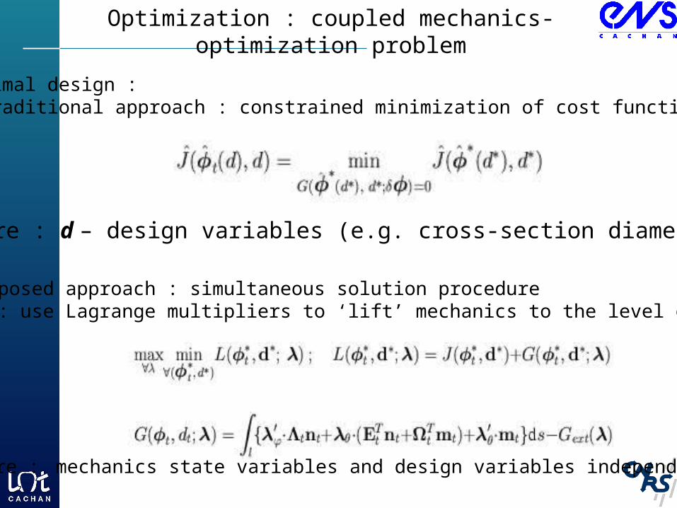
Optimization : coupled mechanics-optimization problem
-where : d – design variables (e.g. cross-section diameter)
ii) Proposed approach : simultaneous solution procedure idea: use Lagrange multipliers to ‘lift’ mechanics to the level of design
-where : mechanics state variables and design variables independent !
-Optimal design :i) Traditional approach : constrained minimization of cost function
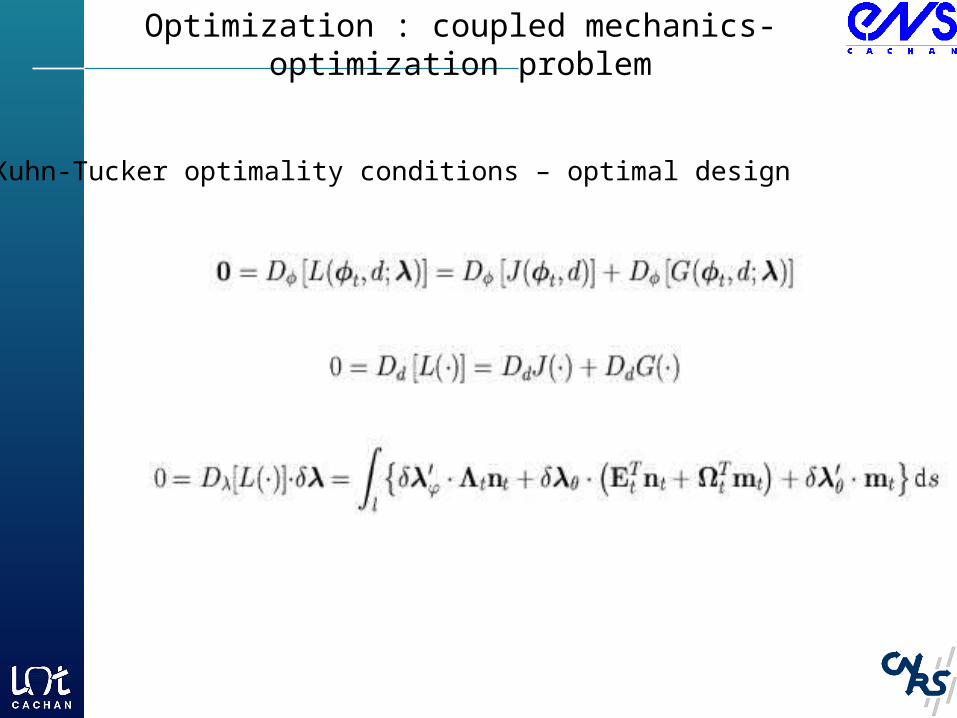
Optimization : coupled mechanics-optimization problem
- Kuhn-Tucker optimality conditions – optimal design

Optimization : coupled mechanics-optimization problem
-Example 1: Cost function – thickness optimization
-Example 2: Cost function – shape optimization
Optimization : coupled mechanics-optimization problem
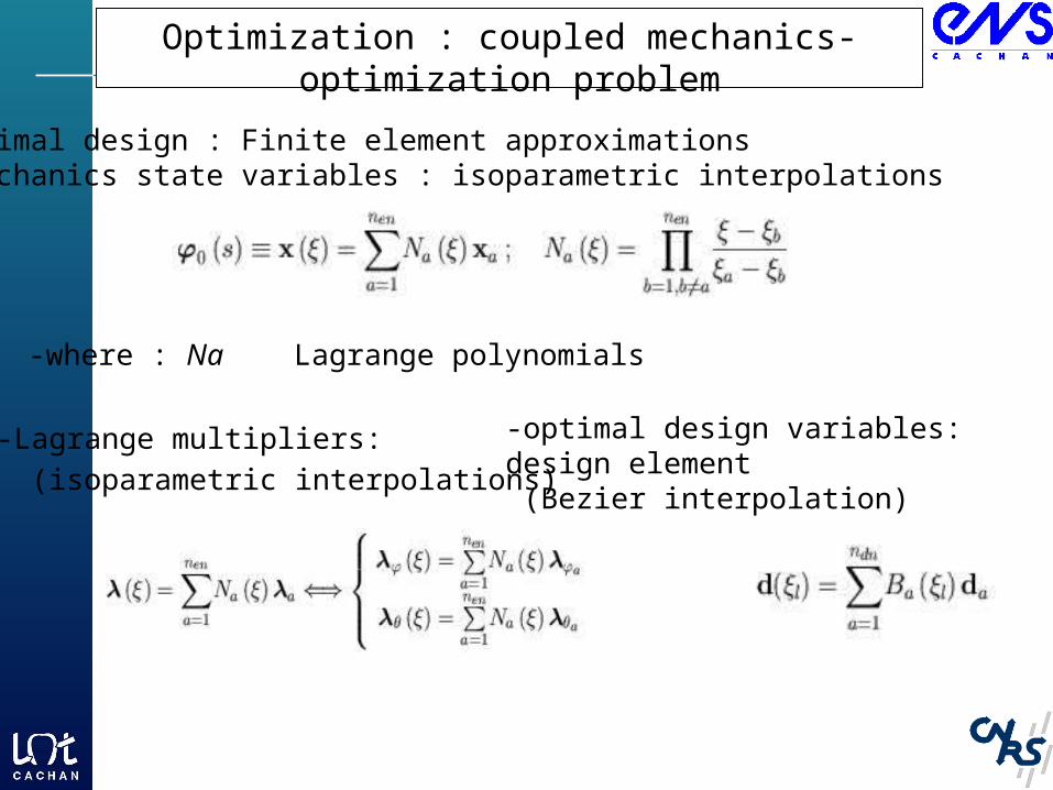
Optimal design : Finite element approximations -mechanics state variables : isoparametric interpolations
-where : Na Lagrange polynomials
-Lagrange multipliers:
(isoparametric interpolations)
-optimal design variables: design element (Bezier interpolation)
Optimization : coupled mechanics-optimization problem
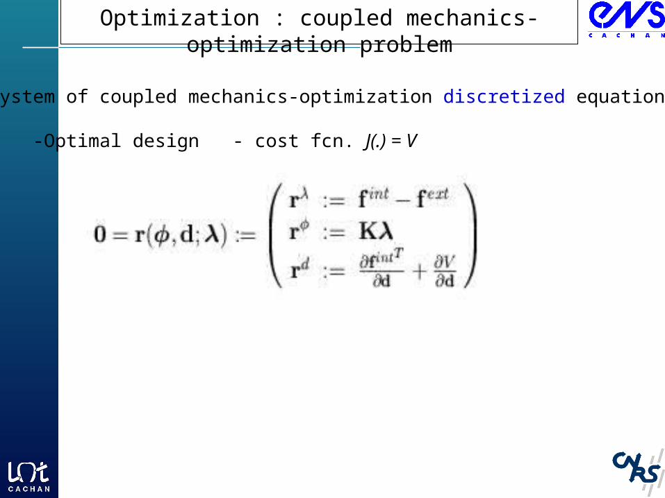
-System of coupled mechanics-optimization discretized equations: -Optimal design - cost fcn. J(.) = V
Optimization : coupled mechanics-optimization problem
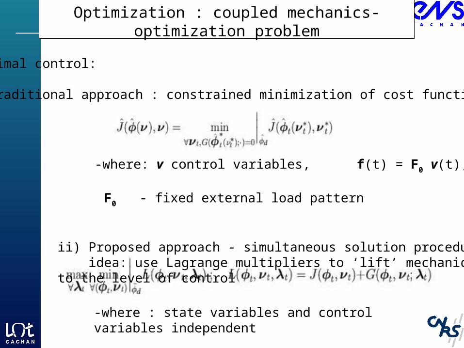
-Optimal control:
i) Traditional approach : constrained minimization of cost function
-where: v control variables, f(t) = F0 v(t) ,
F0 - fixed external load pattern
ii) Proposed approach - simultaneous solution procedure idea: use Lagrange multipliers to ‘lift’ mechanics to the level of control
-where : state variables and control variables independent

Optimization : coupled mechanics-optimization problem
- Kuhn-Tucker optimality conditions – optimal control

Optimization : coupled mechanics-optimization problem
-Example 1: cost function

Optimization : coupled mechanics-optimization problem
- Optimal control: -isoparametric interpolation or “control” elem. -eliminate Lagrange multipliers (if α ≠ 0)
-System of coupled mechanics-control discretized equations:
-Remark: similar to arc-length procedure (tangent plane projection)
Solution procedure for coupled problem
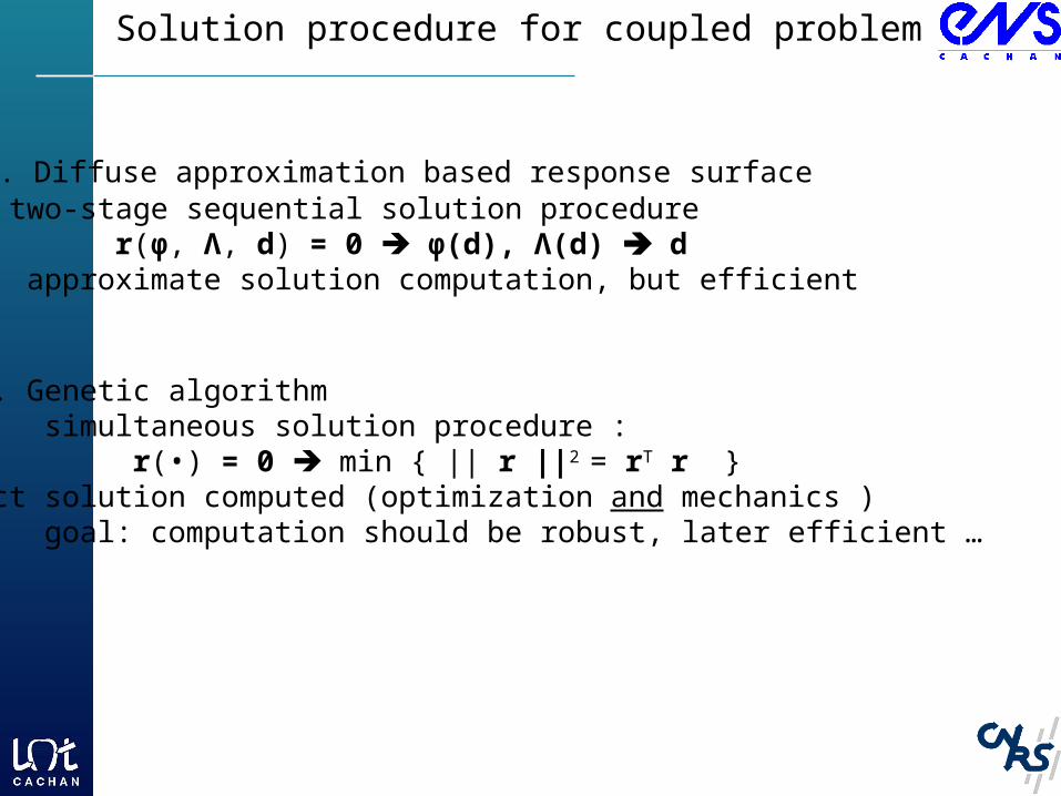
- 1. Diffuse approximation based response surface two-stage sequential solution procedure r(φ, Λ, d) = 0 φ(d), Λ(d) d approximate solution computation, but efficient
- 2. Genetic algorithm simultaneous solution procedure : r(•) = 0 min { || r ||2 = rT r }exact solution computed (optimization and mechanics ) goal: computation should be robust, later efficient …
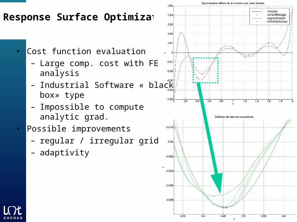
Response Surface Optimization
• Cost function evaluation
– Large comp. cost with FE analysis
– Industrial Software « black box» type
– Impossible to compute analytic grad.
• Possible improvements
– regular / irregular grid
– adaptivity

Diffuse approximation based optimization method
Moving least square – best fit written as minimization problem
First order optimality condition (x – fixed):
-which implies
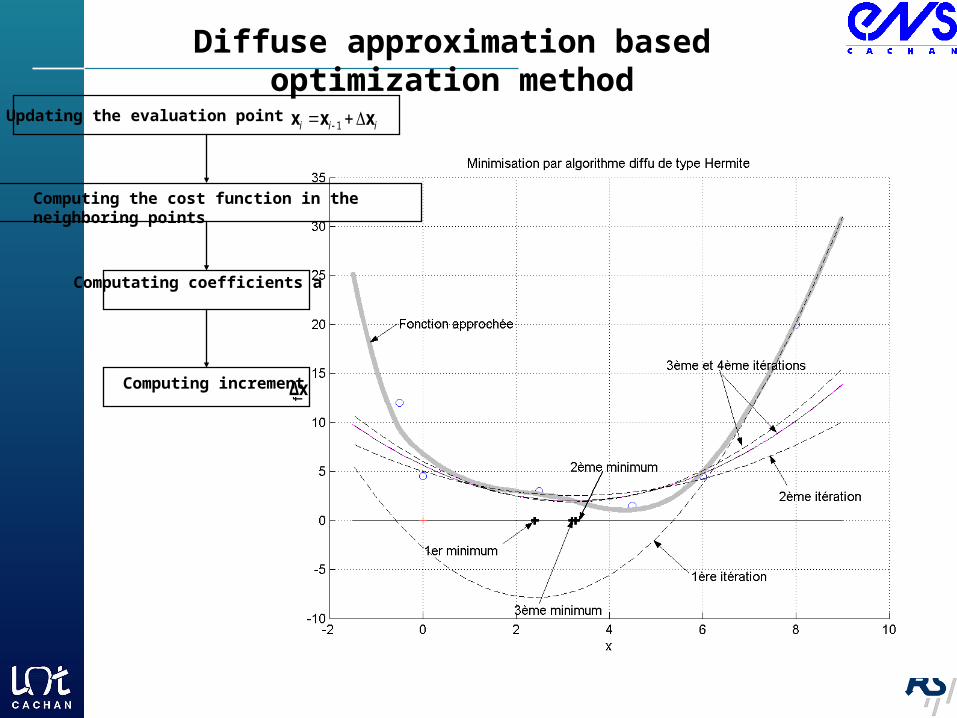
Diffuse approximation based optimization method
iii xxx 1Updating the evaluation point
Computating coefficients a
Computing the cost function in the neighboring points
Computing increment Δx

Shape optimization of cantilever beam
• cost function , constant volume
• discretization with 10 elements : large displacements, large rotations, small strains, elasticity
• shape parameters: 2 quadratic splines
• design variables h(x=0), h(x=l)
dVmises

Genetic algorithm – solution procedure
Solve: r(x) = 0 min { || r ||2 = rT r }• Choose a population of ‘chromosomes’ (size: 10n , n – nb. of eqs.) i-th chromosome of g-th generation :
xi(g) = [ xi1(g), xi2(g),…, xin(g) ]• Producing a new generation: i)-chromosome mutation:
xi(g+1) = xi(g) + MR ( RP - xi(g) )
where: RP = xr(g) – random chromosome; MR – algo. const. ½ ii)-chromosome cross operator:
xi(g+1) = xp(g) + CR ( xq(g) - xr(g) )
where: xp(g), xq(g), xr(g) – randomly chosen chromosomes, CR – radioact. 0.3
ii a)-gradient-like modification of cross operator
xi(g+1) = max(xq(g), xr(g)) + SG CR ( xq(g) - xr(g) ) where: SG – sign selection w/r to gradient iii) tournament of chromosome pairs from two populations reduce population size of generation g+1 again to 10n
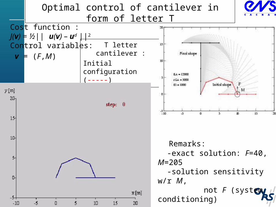
Optimal control of cantilever in form of letter T
T letter cantilever :
Initial configuration (-----)
Final configuration (-----)
Intermediate configs.
Cost function : J(v) = ½|| u(v) – ud ||2
Control variables:
v = (F,M)
Remarks: -exact solution: F=40, M=205 -solution sensitivity w/r M, not F (system conditioning)
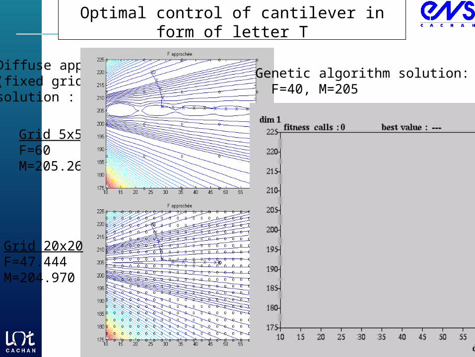
Optimal control of cantilever in form of letter T
Diffuse appr.(fixed grid) solution :
Grid 5x5F=60M=205.26
Grid 20x20F=47.444M=204.970
Genetic algorithm solution: F=40, M=205
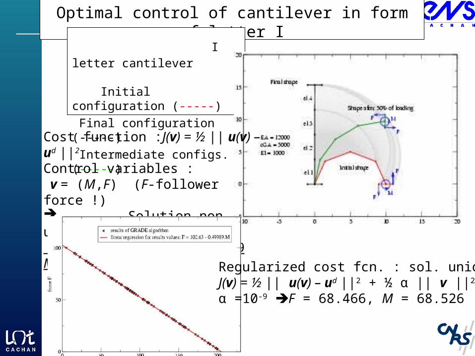
Optimal control of cantilever in form of letter I
I letter cantilever Initial configuration (-----)
Final configuration (-----)
Intermediate configs. (-----)
Cost function :J(v) = ½ || u(v) – ud ||2
Control variables : v = (M,F) (F-follower force !) Solution non-unique : F = 102.63 – 0.49989 M
Regularized cost fcn. : sol. uniqueJ(v) = ½ || u(v) – ud ||2 + ½ α || v ||2 α =10-9 F = 68.466, M = 68.526
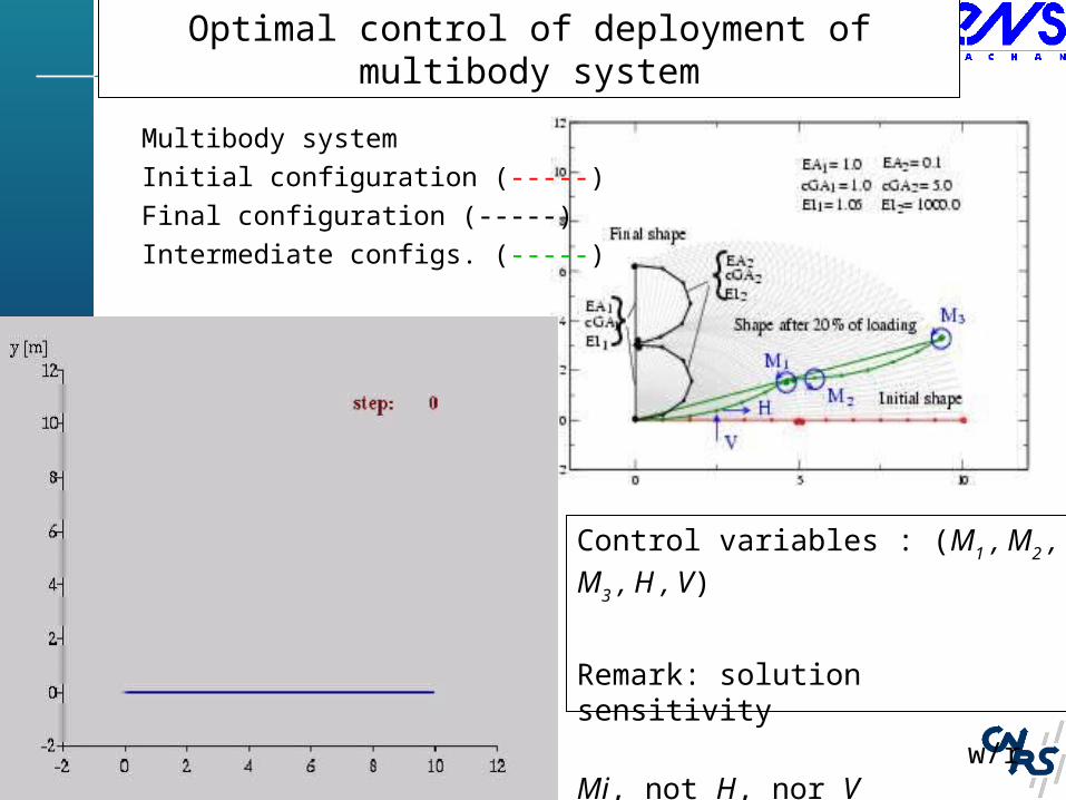
Optimal control of deployment of multibody system
Control variables : (M1 , M2 , M3 , H , V)
Remark: solution sensitivity
w/r Mi, not H, nor V
Multibody system
Initial configuration (-----)
Final configuration (-----)
Intermediate configs. (-----)
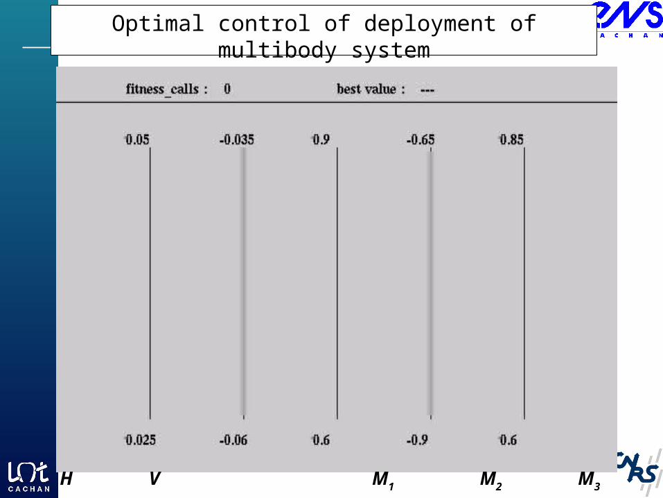
Optimal control of deployment of multibody system
H V M1 M2 M3

Optimal control of deployment of multibody system
1st generation
4th generation
Genetic algorithm basedsolution procedure – moredifficult with larger number of variables
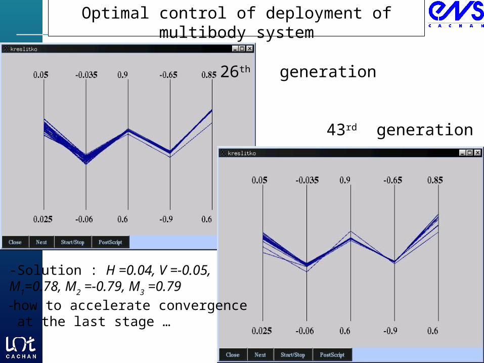
Optimal control of deployment of multibody system
26th generation
43rd generation
-Solution : H =0.04, V =-0.05,M1=0.78, M2 =-0.79, M3 =0.79
-how to accelerate convergence at the last stage …

Conclusions
• Presented unified approach for optimal design and/or control in nonlinear structural mechanics coupled problem opt.-mech.• Model problem : 3D beam – also shells with drills and 3D solids• Solution procedures for solving this optimization problem Response surface algorithm based on diffuse approximation
– generality : without gradients– accuracy : adaptive size of searching pattern– efficiency : progressive construct. of a response surface, reuse of data
points Genetic algorithm simultaneous solution procedure- robustness : solution computed even if non-unique, isolated peak values …- efficiency: to develop further combining with response surface and/or gradient method
To contact me :e-mail : [email protected], fax : +33147402240
:
:
.:
.