localized failure for coupled thermo-mechanics problems: … · 2020-04-29 · adnan ibrahimbegovic...
TRANSCRIPT

HAL Id: tel-00978452https://tel.archives-ouvertes.fr/tel-00978452
Submitted on 14 Apr 2014
HAL is a multi-disciplinary open accessarchive for the deposit and dissemination of sci-entific research documents, whether they are pub-lished or not. The documents may come fromteaching and research institutions in France orabroad, or from public or private research centers.
L’archive ouverte pluridisciplinaire HAL, estdestinée au dépôt et à la diffusion de documentsscientifiques de niveau recherche, publiés ou non,émanant des établissements d’enseignement et derecherche français ou étrangers, des laboratoirespublics ou privés.
Localized failure for coupled thermo-mechanicsproblems : applications to steel, concrete and reinforced
concretevan Minh Ngo
To cite this version:van Minh Ngo. Localized failure for coupled thermo-mechanics problems : applications to steel, con-crete and reinforced concrete. Other. École normale supérieure de Cachan - ENS Cachan, 2013.English. �NNT : 2013DENS0056�. �tel-00978452�

1
ENSC-(n° d’ordre)
THESE DE DOCTORAT
DE L’ECOLE NORMALE SUPERIEURE DE CACHAN
Présentée par
Monsieur NGO Van Minh
pour obtenir le grade de
DOCTEUR DE L’ECOLE NORMALE SUPERIEURE DE CACHAN
Domaine :
MECANIQUE- GENIE MECANIQUE – GENIE CIVIL
Sujet de la thèse :
Localized Failure for Coupled Thermo-Mechanics Problems:
Applications to Steel, Concrete and Reinforced Concrete
Thèse présentée et soutenue à Cachan le 06/12/2013 devant le jury composé de :
Georges CAILLETAUD Professeur, École des Mines, Président du Jury
Luc DAVENNE Maîtres de Conférences, Université Paris Ouest, Rapporteur
Karam SAB Professeur, École des Ponts-ParisTech, Rapporteur
Delphine BRANCHERIE Maîtres de Conférences, UTC, Examineur
Pierre VILLON Professeur , UTC, Examineur
Christophe KASSIOTIS Docteur, ASN, Invité
Amor BOULKERTOUS Docteur, AREVA, Invité
Adnan IBRAHIMBEGOVIC Professeur, ENS Cachan, Directeur de thèse
LMT-Cachan, ENS CACHAN
61, avenue du Président Wilson, 94235 CACHAN CEDEX (France)

2
3
La rupture localisée pour les problèmes couplés thermomécaniques, applications en béton, acier et béton armé

4
Remerciements
Ce travail de thèse s‟est déroulé au sein de la groupe „Construction sous conditions extrêmes‟ du
Secteur Génie Civil, Laboratoire de Mécanique et Technologie (LMT-Cachan), Ecole Normale
Superieure de Cachan. Ces quelques lignes sont dédiées à tous les personnes qui ont contribué de
près ou loin d‟aboutissement de cette thèse, en m‟excusant d‟avance auprès de ceux ou celles que
je n‟aurais pas eu la délicatesse de mentionner.
Mes premiers remerciment vont à Monsieur Adnan Ibrahimbegovic et Madamme Delphine
Brancherie, qui ont initié et encadré mes travaux de thèse. Je leur suis reconnaissant de m‟avoir
accordé leur confiance et d‟avoir su partager leur dynamisme et leur excellence scientifique avec
une grande attention, faisant de nos rencontres des événements toujours stimulants.
Je tiens à remercier Monsieur Georges Cailletaud d'avoir bien voulu, dans une période chargée,
participer à mon jury de thèse et de m'avoir fait l'honneur d'en assurer la présidence. Tous mes
remerciements et un respect profond vont également à ceux qui ont accepté la lourde et
fastidieuse tâche de rapporter ce travail :Monsieur Luc Davenne et Monsieur Karam Sab. Enfin,
je remercie très sincèrement les examinateurs : Monsieur Pierre Villon, Monsieur Christophe
Kassiotis et Monsieur Amor Boulkertous d'avoir accepté de participer à l'examen de ce travail.
Je voudrais également remercier Monsieur Pierre Jehel, qui a été encadré mes travaux de master
avec patience et sympathie.
Je remercie θrofesseur Tran Duc ζhiem, θrofesseur Duong Thi εinh Thu, qui m‟ont démontré
la signification d'être un enseignant et un ingénieur civil.
Je remercie Madamme Nitta Ibrahimbegovic pour les bons dinners et les bons sentiments.
Je remercie mes amis: A. Hung, Hieu, Tien, Son, Pierre, Bahar, Nghia, Miha, Edouard, Mijo,
Emina, Zvonamir, Bobo, He, Cécile, A.Diep, C. Bich, A. Thanh, C.Ngan, A. Cuong, C. Lan, A.
Trang, A. Kien, C.Hoa, C. Thai, Le, A. Hung, C.Hop, Tuan, Lan, Trang, Hung, Thu, Cuong,
Huong,… et beaucoup d‟autres. Je me souviendrai du beau temps avec eux à l‟EζS Cachan.
Enfin, à ma famille et à Sue je decide cette thèse.
5
Lời cảm ơn đến gia đình
Con cảm ơn bố mẹ đã nuôi nấng, dạy bảo, yêu thương, tin tưởng, động viên, chăm sóc con, vợ
chồng con và các cháu trong suốt những năm qua. Cảm ơn bố mẹ đã lo lắng mọi mặt để con có
thể yên tâm bước trên con đường của mình. Kết quả nhỏ này con xin gửi tặng bố mẹ.
Con cảm ơn những tình cảm của bố Quyền, mẹ Hạnh và em Trung; cảm ơn bố mẹ và em Trung
đã luôn ở bên, thông cảm và giúp đỡ con, Quỳnh và các cháu Bin, Sue trong suốt thời gian con
vắng nhà.
Cảm ơn anh chị Nam, Trang và các cháu Bống, Bon đã luôn hỗ trợ, động viên vợ chồng em và
cháu Bin. Không có các bác và các chị, Bin chắc đã buồn hơn rất nhiều khi bố vắng nhà.
Anh cảm ơn sự hi sinh và tình yêu của Quỳnh. Cho tất cả những gì đã xảy ra, anh xin lỗi vì đã
không ở bên em quá lâu và cảm ơn em đã chăm sóc bố mẹ, chăm sóc các con. Cảm ơn em đã đọc
và sửa từng dòng trong quyển luận văn này. Cảm ơn em đã theo dõi từng bước đi, đã vui khi anh
có một vài kết quả nhỏ, đã buồn khi anh gặp khó khăn và đã tha thứ mỗi khi anh làm em buồn.
Cảm ơn em đã đem Bin và Sue đến trong cuộc sống của chúng ta.
Luận văn này hoàn thành là lúc ba có thể về chơi ô tô với anh Bin và đón chào sự ra đời của em
Sue như ba đã hứa. Ba mẹ và anh Bin tặng luận văn này cho em Sue, thành viên mới trong một
gia đình nhỏ mà từ nay sẽ luôn ở gần bên nhau. Ba hứa với các con là chúng ta sẽ ở bên nhau,
chắc chắn là như vậy.

6
Abstract
During the last decades, the localized failure of massive structures under thermo-mechanical
loads becomes the main interest in civil engineering due to a number of construction damaged
and collapsed due to fire accident. Two central questions were carried out concerning the
theoretical aspect and the solution aspect of the problem.
In the theoretical aspect, the central problem is to introduce a thermo-mechanical model capable
of modeling the interaction between these two physical effects, especially in localized failure.
Particularly, we have to find the answer to the question: how mechanical loading affect the
temperature of the material and inversely, how thermal loading result in the mechanical response
of the structure. This question becomes more difficult when considering the localized failure
zone, where the classical continuum mechanics theory can not be applied due to the discontinuity
in the displacement field and, as will be proved in this thesis, in the heat flow.
In terms of solution aspect, as this multi-physical problem is mathematical represented by a
differential system, it can not be solved by an „exact‟ analytical solution and therefore, numerical
approximation solution should be carried out.
This thesis contributes to both of these two aspects. Particularly, thermomechanical models for
both steel and concrete (the two most important materials in civil engineering), which capable of
controling the hardening behavior due to plasticity and/or damage and also the softening
behavior due to the localized failure, are carried out and discussed. Then, the thermomechanical
problems are solved by „adiabatic‟ operator split procedure, which „separates‟ the multi-physical
process into the „mechanical‟ part and the „thermal‟ part. Each part is solved individually by
another operator split procedure in the frame-work of embbed-discontinuity finite element
method. In which, the „local‟ discontinuities of the displacement field and the heat flow is solved
in the element level, for each element where localized failure is detected. Then, these
discontinuities are brought into the „static condensation‟ form of the overall equilibrium
equation, which is used to solved the displacement field and the temperature field of the structure
at the global level.
The thesis also contributes to determine the ultimate response of a reinforced concrete frame
submitted to fire loading. In which, we take into account not only the degradation of material
properties due to temperature but also the thermal effect in identifying the total response of the
7
structure. Moreover, in the proposed method, the shear failure is also considered along with the
bending failure in forming the overal failure of the reinforced structure.
The thesis can also be extended and completed to solve the behavior of reinforced concrete in 2D
or 3D case considering the behavior bond interface or to take into account other type of failures
in material such as fatigue or buckling. The proposed models can also be improved to determine
the dynamic response of the structure when subjected to earthquake and/or impact.

8
Résumé
Ces dernières années, l'étude de la rupture localisée des structures massives sous chargement
thermomécanique est devenue un enjeu important en Génie Civil du fait de l'augmentation du
nombre de constructions endommagées ou totalement effondrées après un feu. Deux questions
centrales ont émergé: la modélisation mathématique des phénomènes mis en jeu lors d'un feu
d'une part et la simulation numérique de ces problèmes d'autre part.
Concernant la modélisation mathématique, la principale difficulté est la mise en place de
modèles thermomécaniques capables de modéliser le couplage existant entre les effets
thermiques et mécaniques, en particulier dans une zone de rupture localisée. Comment le
chargement mécanique affecte la distribution de température dans le matériau et inversement,
comment le chargement thermique influence la réponse mécanique? Sont des questions qui
doivent être abordées. Ces questions sont d'autant plus difficiles à aborder que l'on considère une
zone de rupture où la mécanique des milieux continus classiques ne peut pas être appliquée du
fait de la présence de discontinuités du champ de déplacement et, comme cela est démontré dans
ce travail, du flux thermique.
Pour ce qui concerne la simulation numérique, la complexité du problème multi-physique posé
en termes de système d'équations aux dérivées partielles impose le développement de méthodes
de résolution approchées adaptées, efficaces et robustes, la solution analytique n'étant en général
pas disponible.
Cette thèse contribue sur tous les deux aspects précédents. En particulier, des modèles
thermomécaniques pour le béton et l'acier (les deux principaux matériaux utilisés en Génie Civil)
capables de contrôler simultanément les phases d'écrouissage accompagnées de plasticité et/ou
d'endommagement diffus, ainsi que la phase adoucissante due au développement de macro-
fissures, sont proposés. Le problème thermomécanique est ensuite résolu par une méthode dite
«adiabatic operator split» qui consiste à séparer le problème multiphysique en une partie
mécanique et une partie thermique. Chaque partie est résolue séparément en utilisant une fois de
plus une méthode «d'operator split» dans le cadre des méthodes à discontinuités fortes. Dans ces
dernières, une discontinuité du champ de déplacement ou du flux thermique est introduite et
gérée au niveau élémentaire du code de calcul Éléments Finis. Une procédure de condensation
statique élémentaire permet de prendre en compte ces discontinuités sans modification de
9
l'architecture globale du code de calcul Éléments Finis fournissant les champs de déplacement et
de température.
Dans cette thèse est également abordée la question de l'évaluation de la réponse jusqu'à rupture
de structures en béton armé de type poteaux/poutres soumises à un feu. L'originalité de la
formulation proposée est de tenir compte de la dégradation des propriétés mécaniques du
matériau due au chargement thermique pour la détermination de la résistance limite et résiduelle
des structures, mais également de prendre en compte deux types de rupture caractéristiques des
structures poteaux/poutres à savoir les ruptures en flexion et les ruptures en cisaillement.
Les travaux présentés dans cette thèse pourront être étendus pour décrire la rupture de structures
en béton armé dans des cas bi ou tridimensionnels en tenant compte en particulier du
comportement de l'interface acier/béton et/ou d'autres types de rupture comme la rupture par
fatigue ou le flambage. Une extension possible est également la prise en compte des effets
dynamiques mis en jeu lorsque la structure est sollicitée mécaniquement par un tremblement de
terre ou un impact en plus de la sollicitation thermique.

10
Table of Contents
Remerciements .............................................................................................................................................. 4
Lời cảm ơn đến gia đình ............................................................................................................................... 5
Abstract ......................................................................................................................................................... 6
Résumé .......................................................................................................................................................... 8
Table of Figures .......................................................................................................................................... 13
List of Tables .............................................................................................................................................. 16
List of Publications ..................................................................................................................................... 17
Journals ................................................................................................................................................... 17
Conferences and Workshops .................................................................................................................. 17
1 Introduction ........................................................................................................................................ 18
1.1 Problem statement and its importance ........................................................................................ 18
1.2 Literature review ......................................................................................................................... 20
1.2.1 Previous works on stress-resultant model ........................................................................... 21
1.2.2 Previous works on multi-dimensional thermodynamics model .......................................... 22
1.3 Aims, scope and method ............................................................................................................. 24
1.4 Outline......................................................................................................................................... 25
2 Thermo-plastic coupling behavior of steel: one-dimensional simulation .......................................... 27
2.1 Introduction ................................................................................................................................. 27
2.2 Theoretical formulation of localized thermo-mechanical coupling problem .............................. 29
2.2.1 Continuum thermo-plastic model and its balance equation ................................................ 29
2.2.2 Thermodynamics model for localized failure and modified balance equation. .................. 32
2.3 Embedded-Discontinuity Finite Element Method (ED-FEM) implementation .......................... 36
2.3.1 Domain definition ............................................................................................................... 36
2.3.2 „Adiabatic‟ operator splitting solution procedure ............................................................... 37
2.3.3 Embedded discontinuity finite element implementation for the mechanical part ............... 38
2.3.4 Embedded discontinuity finite element implementation for the thermal part ..................... 44

11
2.4 Numerical simulations ................................................................................................................ 47
2.4.1 Simple tension imposed temperature example with fixed mesh ......................................... 47
2.4.2 Mesh refinement, convergence and mesh objectivity ......................................................... 61
2.4.3 Heating effect of mechanical loading ................................................................................. 62
2.5 Conclusions ................................................................................................................................. 64
3 Behavior of concrete under fully thermo-mechanical coupling conditions ....................................... 66
3.1 Introduction ................................................................................................................................. 66
3.2 General framework ..................................................................................................................... 67
3.2.1 General continuum thermodynamic model ......................................................................... 67
3.2.2 Localized failure in damage model ..................................................................................... 71
3.2.3 Discontinuity in the heat flow ............................................................................................. 75
3.2.4 System of local balance equation ........................................................................................ 76
3.3 Finite element approximation of the problem ............................................................................. 76
3.3.1 Finite element approximation for displacement field ......................................................... 76
3.3.2 Finite element interpolation function for temperature ........................................................ 77
3.3.3 Finite element equation for the problem ............................................................................. 79
3.4 Operator split solution procedure ................................................................................................ 82
3.4.1 Mechanical process ............................................................................................................. 83
3.4.2 Thermal process .................................................................................................................. 88
3.5 Numerical Examples ................................................................................................................... 90
3.5.1 Tension Test and Mesh independency ................................................................................ 91
3.5.2 Simple bending test ............................................................................................................. 95
3.5.3 Concrete beam subjected to thermo-mechanical loads ....................................................... 99
3.6 Conclusion ................................................................................................................................ 103
4 Thermomechanics failure of reinforced concrete frames ................................................................. 104
4.1 Introduction ............................................................................................................................... 104

12
4.2 Stress-resultant model of a reinforced concrete beam element subjected to mechanical and
thermal loads......................................................................................................................................... 105
4.2.1 Stress and strain condition at a position in reinforced concrete beam element under
mechanical and temperature loading. ............................................................................................... 105
4.2.2 Response of a reinforced concrete element under external loading and fire loading. .............
112
4.2.3 Effect of temperature loading, axial force and shear load on mechanical moment-curvature
response of reinforced concrete beam element. ............................................................................... 116
4.2.4 Compute the mechanical shear load – shear strain response of a reinforced concrete
element subjected to pure shear loading under elevated temperature .............................................. 119
4.3 Finite element analysis of reinforced concrete frame ............................................................... 122
4.3.1 Timoshenko beam with strong discontinuities .................................................................. 122
4.3.2 Stress-resultant constitutive model for reinforced concrete element ................................ 125
4.3.3 Finite element formulation ................................................................................................ 130
4.4 Numerical example ................................................................................................................... 137
4.4.1 Simple four-point bending test .......................................................................................... 137
4.4.2 Reinforced concrete frame subjected to fire ..................................................................... 141
4.5 Conclusion ................................................................................................................................ 146
5 Conclusions and Perpectives ............................................................................................................ 147
5.1 Main contributions .................................................................................................................... 147
5.2 Perpectives ................................................................................................................................ 148
6 Bibliography ..................................................................................................................................... 149
13
Table of Figures
Figure 1-1. Windsor Tower (Madrid) before, in and after fire disater ......................................................................... 20
Figure 1-2. Stress-resultant model of a reinforced concrete structure ........................................................................ 21
Figure 2-1.Displacement discontinuity at localized failure for the mechanical load ................................................... 33
Figure 2-2.Displacement discontinuity for 2-node bar element: Heaviside function a d φ x .............................. 34
Figure 2-3. Heterogeneous two-phase material for a truss bar, with phase-interface placed at ............................. 36
Figure 2-4.Two sub-domain � 1 and � 2 separated by localized failure point at .................................................. 37
Figure 2-5Displacement discontinuity shape function M1(x) and its derivative. .......................................................... 39
Figure 2-6. Strain discontinuity shape function M2 and its derivative ........................................................................ 39
Figure 2-7. Bar subjected to imposed displacement and temperature applied simultaneously .................................. 47
Figure 2-8. Time variation of imposed displacement and temperature ...................................................................... 48
Figure 2-9. Stress– strain curves in two sub-domains .................................................................................................. 50
Figure 2-10. Force – displacement curve of the bar ..................................................................................................... 50
Figure 2-11. Distribution of temperature (oC) along the bar at chosen values of time ................................................ 51
Figure 2-12. Evolutio of Δ versus time (in 0C) ......................................................................................................... 52
Figure 2-13. Stress-strain curves in two sub-domains ................................................................................................. 53
Figure 2-14. Force displacement curve ........................................................................................................................ 53
Figure 2-15. Evolution of temperature (oC) along the bar in time ............................................................................... 54
Figure 2- 6. Evolutio of Δϑ versus time (in 0C) ........................................................................................................... 55
Figure 2-17.Temperature dependent coefficients (according to [6]) ........................................................................... 57
Figure 2-19. Force-displacement diagram for the bar ................................................................................................. 58
Figure 2-18. Stress-strain curvesfor two sub-domains ................................................................................................. 58
Figure 2-20. Distribution of temperature (0C) along the bar due to time .................................................................... 59
Figure 2- . Evolutio of Δϑ vs time ............................................................................................................................ 60
Figure 2-22.Bar subjected to imposed loading and imposed temperature ................................................................. 61
Figure 2-23. Load-displacement diagram with different number of elements ............................................................ 62
Figure 2-25. Load-displacement curve ......................................................................................................................... 63
Figure 2-24. Description of the third example and its mesh ........................................................................................ 63
Figure 2-26. Temperature evolution along the bar before and after the localized failure occurs (computed with 5
elements mesh) ............................................................................................................................................................ 64
14
Figure 2-27. Temperature evolution along the bar before and after the localized failure occurs (computed with 9
elements mesh) ............................................................................................................................................................ 64
Figure 3-1. Lo alized failure happe s at ra k surfa e a d the lo al zo e .............................................................. 71
Figure 3-2. Additional shape function M1(x) for displacement discontinuity ............................................................... 77
Figure 3-3. Additional shape function .......................................................................................................................... 78
Figure 3-4. Adia ati splitti g pro edure. ................................................................................................................ 83
Figure 3-5. Local computation for mechanical part ..................................................................................................... 86
Figure 3-6. Temperature distribution in the plate at t = 20s ........................................................................................ 92
Figure 3-7. Temperature distribution in the plate at t = 52.4s..................................................................................... 92
Figure 3-8. Temperature distribution in the plate at t = 100s...................................................................................... 92
Figure 3-9. Load/Displacement Curve for the coarse and the fine mesh ..................................................................... 93
Figure 3-10. Traction - Crack Opening relation at the localized failure ....................................................................... 93
Figure 3-11. Load/ Displacement Curve of the plate in thermo-mechanical loadings ................................................. 95
Figure 3-12. Temperature evolution in the plate for the first loading case (0C) .......................................................... 97
Figure 3-13. Temperature evolution in the plate for the second loading case (0C) ..................................................... 97
Figure 3-14. Evolution of maximum principal stress for the first loading case (MPa) ................................................. 98
Figure 3-15. Evolution of maximum principal stress for the second loading case (MPa) ............................................ 98
Figure 3-16. Load/ Displacement curve for 2 loading cases ........................................................................................ 98
Figure 3-17. Example configuration ............................................................................................................................. 99
Figure 3-18. Evolution of maximum principal stress and temperature due to time .................................................. 100
Figure 3-19. State of the plate at the final loading stage (t = 20s) ............................................................................ 101
Figure 3-20. Mechanical and Thermal state of the plate after unloading (t=40s) ..................................................... 101
Figure 3-21. Reaction/ Deflection curve .................................................................................................................... 102
Figure 4-1. Mechanical loading and fire acting on reinforced concrete element ...................................................... 106
Figure 4-2. Thermal stress and thermal strain condition ........................................................................................... 106
Figure 4-3. Total stress and strain condition at a positio i ea ele e t εy= a d σy=0) ................................... 107
Figure 4-4. Mohr circle representation for strain and stress condition at a point in beam element ......................... 108
Figure 4-5. Relation between compressive stress and strain of concrete due to tempeture[10] .............................. 110
Figure 4-6. Stress- strain relationship of rebar in different temperature................................................................... 112
Figure 4-7. Response of reinforced concrete element under mechanical and thermal loads .................................... 113
15
Figure 4-8. Procedure to determine the mechanical response of RC beam element ................................................. 115
Figure 4-9. Cross-section and Dimensioning of the consider reinforced concrete element ....................................... 116
Figure 4-10. Evolution of temperature profile due to time[11] ................................................................................. 116
Figure 4-11. Dependence of moment-curvature with time exposure to fire ASTM119 ............................................. 117
Figure 4-12. Dependence of moment-curvature on axial compression ..................................................................... 117
Figure 4-13. Dependence of moment-curvature response on shear loading ............................................................. 118
Figure 4-14. Multi-linear moment-curvature model of the reinforced concrete beam in bending ............................ 119
Figure 4-15. Stress components of reinforced concrete subjected to pure shear loading ......................................... 120
Figure 4-16. Mechanical shear force- shear deformation diagram ........................................................................... 121
Figure 4-17. Beam under external loading and fire ................................................................................................... 122
Figure 4-18. Kinematic of beam element ................................................................................................................... 124
Figure 4-19. Moment-curvature relation for bending stress-resultant model ........................................................... 128
Figure 4-20. Shear load-shear strain relation for shear stress-resultant model ........................................................ 130
Figure 4-21. Simple reinforced concrete beam subjected to ASTM 119 fire and vertical forces ................................ 137
Figure 4-22. Reduction of bending resistance due to time exposing to fire ASTM 119 ............................................. 138
Figure 4-23. Reduction of shear resistance due to time exposing to fire ASTM 119 ................................................. 139
Figure 4-24. Force/displacement curve of the beam at different instants of fire loading program .......................... 140
Figure 4-25. Reduction of ultimate load due to fire exposure ................................................................................... 141
Figure 4-26. Two-story reinforced concrete frame subjected to loading and fire ..................................................... 142
Figure 4-27. Temperature profile of the reinforced concrete beam due to time of fire ............................................. 143
Figure 4-28. Moment-curvature model for column ................................................................................................... 144
Figure 4-29. Shear failure model of the column......................................................................................................... 144
Figure 4-30. Degradation of bending resistance of reinforced concrete beam versus fire exposure......................... 145
Figure 4-31.Horizontal force/displacement curve of two-story frame at different instants of fire ........................... 145

16
List of Tables
Table 1-1. Several building fire accidents from 1970 to present (see [4]).................................................................... 19
Table 2-1. Material properties of steel bar .................................................................................................................. 49
Table 2-2.Time Evolution of Temperature along the Bar ............................................................................................. 51
Table 2-3.Time evolution of temperature along the bar ............................................................................................. 54
Table 2-4. Temperature dependent coefficients .......................................................................................................... 56
Table 2-5. Distribution of temperature along the bar ................................................................................................. 59
Table 2-6. Material properties ..................................................................................................................................... 61
Table 3-1. Material Properties .................................................................................................................................... 91
Table 4-1. List of symbols for thermomechanical model ........................................................................................... 105
Table 4-2. Bending model parameters for different instants of fire loading program .............................................. 138
Table 4-3. Parameters of shear model at different instants of fire loading program ................................................ 139
Table 4-4. Material properties ................................................................................................................................... 143

17
List of Publications
Journals
[1] V.M. Ngo, A. Ibrahimbegovic, and D. Brancherie, "Model for localized failure with thermo-plastic
coupling. Theoretical formulation and ED-FEM implementation," Computers and Structures, vol. 127,
pp. 2-18, 2013.
[2] M. Ngo, A. Ibrahimbegovic, and D. Brancherie, "Continuum damage model for thermo-mechanical
coupling in quasi-brittle materials," Engineering Structure, vol. 50, pp. 170-178, 2013.
[γ] ε. ζgo, A. Ibrahimbegovic, and D. Brancherie, “Softening behavior of quasi-brittle material under
full thermo-mechanical coupling condition: Theoretical formulation and finite element implementation,”
Computer Methods in Applied Mechanics and Engineering, Accepted.
[4] N.N Bui, M. Ngo, D. Brancherie, and A. Ibrahimbegovic, "Enriched Timoshenko beam finite element
for modelling bending and shear failure of reinforced concrete frames," Computer and Structures,
Submitted.
[5] ε. ζgo, A. Ibrahimbegovic, and D. Brancherie, “Thermomechanics Failure of Reinforced Concrete
Composites: Computational Approach with Enhanced Beam Model,” Computer and Concretes,
Submitted.
[6] M.Ngo, A. Ibrahimbegovic and E. Hajdo, “δocalized failure for large deformation of thermo-plasticity
problem,” Nonlinear Coupled Mechanic System, Submitted.
Conferences and Workshops
1. V.M. Ngo, P. Jehel, A. Ibrahimbegovic “Numerical modelling of monotonic and cyclic response of
anchorage steel bar,” Workshop on Construction under Exceptional Conditions (CEC 2010),
Hanoi,October, 2010.
2. M. Ngo, A. Ibrahimbegovic, and D. Brancherie , “A thermo-damage coupling model for concrete
structure,” 7th International Conference on Computational Mechanics for Spatial Structures. IASS-IACM
2012, Sarajevo, April 2-4, 2012.
3. M. Ngo, A. Ibrahimbegovic, and D. Brancherie “Continuum damage model for thermo-mechanical
coupling in quasi-brittle materials,” The first AVSE Annual Doctoral Workshop. ENS Cachan, Cachan,
September 13-14, 2012.
Chapter 1. Introduction
18
1 Introduction
1.1 Problem statement and its importance
The characterization of the failure in steel, concrete and reinforced concrete structures under
thermo-mechanical loading is not only the main theoretical importance but also the major
interest for its practical application. In recent years, the number of massive constructions
collapsed and/or damaged due to fire loading is increasing. A list of several major building fire
accidents from 1970 onwards (given in Table 1-1) has indicated the progress of them in term of
number and severity. Among these accidents, perhaps the most well-known is the collapse of the
World Trade Centre in New York in September, 2001, where the thermal response and the
degradation of material properties due to fire were considerably contributed into the final
breakdown of the tower in addition to the mechanical response due to the airplane impact (see
[1], [2], [3]). More recently, the burning occurred in the 32-storey Windsor tower in Madrid,
Spain in February, 2005 (see Figure 1-1) is also a typical example of construction failure due to
fire loading. In this accident, the fire started on the 21st floor then quickly spread throughout the
entire building. After 24 hours exposure to fire, the steel components of the tower were
destroyed while the reinforced concrete components were also partially damaged. Although not
being completely destroyed in the fire, the remaining reinforced concrete structures had also lost
its working capacity and had to be demolished later. These structural failures, from the civil
engineering point of view, happened due to the lack of structure resistance, or more particularly,
the degradation of structure resistance when exposed to extreme thermal loads. This issue is still
not clearly understood presently. Therefore, it is necessary to go into deeper studies of the
behavior of structure subjected to thermal loading and mechanical loading simultaneously. Of
special interest is the problem of localized failure of the structure at extreme conditions that can
produce the localized heavily damaged zones leading to structure softening response. In this
thesis, the localized failure of structures built of standard construction materials, such as steel,
concrete and reinforced concrete will be discussed. The main target, as will be explained in more
detail in the following, is to provide a more robustness simulation of the „ultimate‟ response of
reinforced concrete structure, which will further lead to a better and safer design of the
construction.
Localized Failure for Coupled Thermo-Mechanics Problems
19
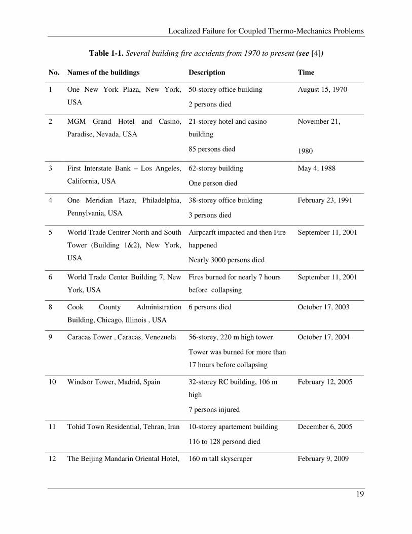
Table 1-1. Several building fire accidents from 1970 to present (see [4])
No. Names of the buildings Description Time
1 One New York Plaza, New York,
USA
50-storey office building
2 persons died
August 15, 1970
2 MGM Grand Hotel and Casino,
Paradise, Nevada, USA
21-storey hotel and casino
building
85 persons died
November 21,
1980
3 First Interstate Bank – Los Angeles,
California, USA
62-storey building
One person died
May 4, 1988
4 One Meridian Plaza, Philadelphia,
Pennylvania, USA
38-storey office building
3 persons died
February 23, 1991
5 World Trade Centrer North and South
Tower (Building 1&2), New York,
USA
Airpcarft impacted and then Fire
happened
Nearly 3000 persons died
September 11, 2001
6 World Trade Center Building 7, New
York, USA
Fires burned for nearly 7 hours
before collapsing
September 11, 2001
8 Cook County Administration
Building, Chicago, Illinois , USA
6 persons died October 17, 2003
9 Caracas Tower , Caracas, Venezuela 56-storey, 220 m high tower.
Tower was burned for more than
17 hours before collapsing
October 17, 2004
10 Windsor Tower, Madrid, Spain 32-storey RC building, 106 m
high
7 persons injured
February 12, 2005
11 Tohid Town Residential, Tehran, Iran 10-storey apartement building
116 to 128 persond died
December 6, 2005
12 The Beijing Mandarin Oriental Hotel, 160 m tall skyscraper February 9, 2009

Chapter 1. Introduction
20
Figure 1-1. Windsor Tower (Madrid) before, in and after fire disater
1.2 Literature review
There are two types of structural analysis that can be used in determining the behavior of steel,
concrete and reinforced concrete structures, which are the (one-dimensional) stress-resultant
model and the multi-dimensional continuum mechanics model. In dealing with these problems in
the most efficient manner, we are led to develop different both the continuum-mechanics-based
models and the stress resultant models.
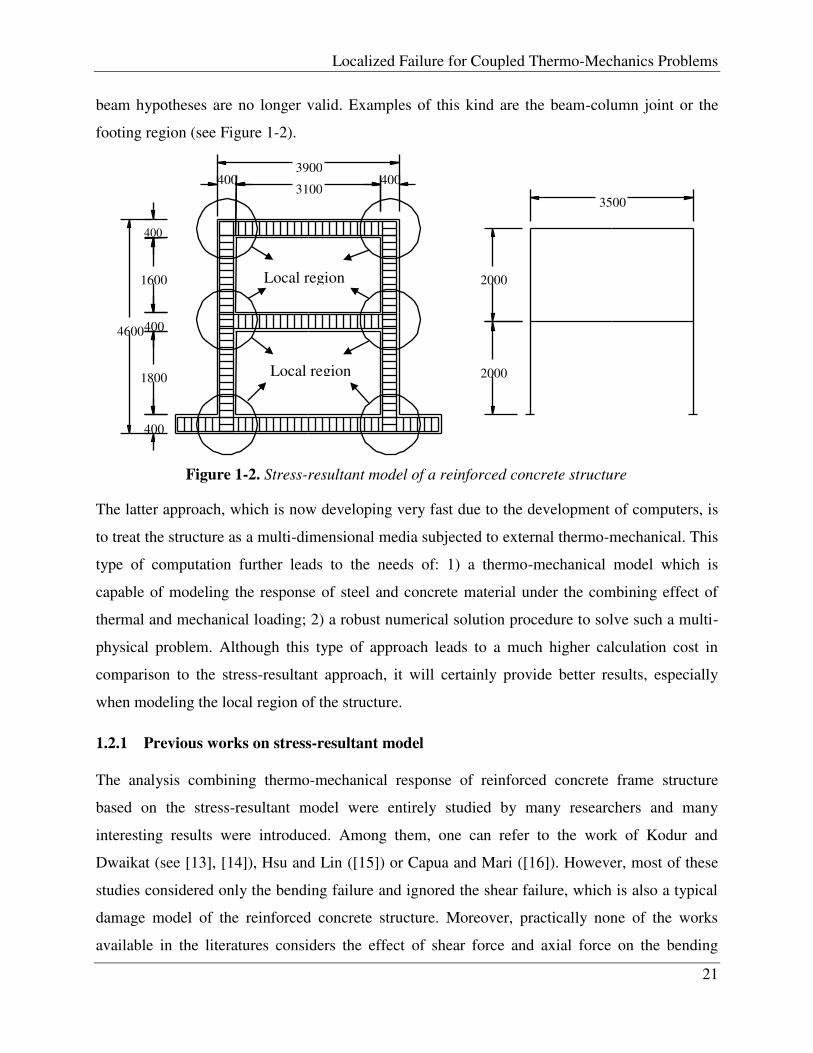
The stress resultant model considers the structure as a system of one-dimensional elements:
beams, frames, columns, trusses. (see Figure 1-2). These elements, due to their special
configurations with one dimension being much greater than the two others, are assumed to
satisfy traditional hypotheses of the structural analysis such as the Saint-Venant hypothesis:
„…the difference between the effects of two different but statically equivalent loads becomes very
small at sufficiently large distances from load‟ (see [5]) and the beam theory assumptionsμ „beam
is initial straight and has a constant cross-section‟, „the plane cross-section remains plane
before and afterloading‟. Due to the simplicity and the low-cost of computation, this type of
approach is widely used in practical design of reinfored concrete as well as steel structures
submitted to combined action of fire and mechanical loading. Such is still the basic method
introduced in the design code of Europe and America nowadays (see [6],[7], [8], [9], [10], [11]).
However, despite the forementioned avantages, the stress-resultant model can not be applied for
the „local‟ regions (or the „D‟ regions [12], [9]) of the structure where the Saint-Venant and
Localized Failure for Coupled Thermo-Mechanics Problems
21
beam hypotheses are no longer valid. Examples of this kind are the beam-column joint or the
footing region (see Figure 1-2).
The latter approach, which is now developing very fast due to the development of computers, is
to treat the structure as a multi-dimensional media subjected to external thermo-mechanical. This
type of computation further leads to the needs of: 1) a thermo-mechanical model which is
capable of modeling the response of steel and concrete material under the combining effect of
thermal and mechanical loading; 2) a robust numerical solution procedure to solve such a multi-
physical problem. Although this type of approach leads to a much higher calculation cost in
comparison to the stress-resultant approach, it will certainly provide better results, especially
when modeling the local region of the structure.
1.2.1 Previous works on stress-resultant model
The analysis combining thermo-mechanical response of reinforced concrete frame structure
based on the stress-resultant model were entirely studied by many researchers and many
interesting results were introduced. Among them, one can refer to the work of Kodur and
Dwaikat (see [13], [14]), Hsu and Lin ([15]) or Capua and Mari ([16]). However, most of these
studies considered only the bending failure and ignored the shear failure, which is also a typical
damage model of the reinforced concrete structure. Moreover, practically none of the works
available in the literatures considers the effect of shear force and axial force on the bending
Figure 1-2. Stress-resultant model of a reinforced concrete structure
Local region 2000
2000
3500
400
3900
400
1800
400
1600
4600
400 3100
400
Local region

Chapter 1. Introduction
22
resistance of reinforced concrete element, although the stress-strain relation of the cross-section
where shear force and axial force exist are much different from the stress/strain condition of the
pure bending cross-section. Another deficiency of previously proposed methods is that only the
degradation of the mechanical resistance due to material strength reduction at high temperature is
taken into account, while the „thermal‟ response of the frame is usually neglected while at high
temperature, thermal behavior might significantly contribute to the total behavior of the section.
The last important model feature to be improved with respect to the previous works is to cast the
stress-resultant model that can represent such a thermomechanical behavior of a reinforced
concrete elements (either beam or column), which can provide an efficient computational basis
in identifying the overall response of the frame structure. Therefore, a method to overcome the
mentioned shortcomings of the present stress-resultant based model will be introduced in this
thesis.
1.2.2 Previous works on multi-dimensional thermodynamics model
As already declared, the multi-dimensional analysis of „local‟ regions should be based on a
thermo-mechanical model of steel and concrete material. In the following, some main
contributions on the modeling of softening behavior of construction material due to mechanical
effect only and due to thermo-mechanical coupling effect are summarized.
The „ultimate‟ resistance of structures under mechanical loading was previously studied by many
research groups, by using a number of different approaches. The research group entitled
„Structure under Extreme Conditions‟ of θrofessor Ibrahimbegovic at δεT Cachan contributed
to this topic by considering the softening behavior of material in the frame-work of Embedded-
Discontinuity Finite Element Method (see [17]). Here, the localized failure of the solid is
represented as a „discontinuity‟ (or a „jump‟) in displacement field and is modeled by an
additional interpolation function using the incompatible mode in finite element method [18].
Based on this method, this research group contributed in determining the softening behavior of
the structure due to both the stress-resultant model approach and the multi-dimensional analysis
approach. For the stress-resultant model approach, one can refer to the study on the bending
failure frame (see [19],[20]) and/or the bending failure accompanied with shear failure (see [21])
of reinforced concrete frame. In terms of the multi-dimensional analysis approach, the
thermomechanical softening model of some fundamental construction materials were introduced:
Localized Failure for Coupled Thermo-Mechanics Problems
23
elasto-plastic steel material structure (see [22],[23]), quasi-brittle material (concrete, masonry)
(see [24], [25]) and reinforced concrete structures (see [26]). Other (and earlier) significant
contributions to the topic that should be recalled are the work of Ortiz el al. on weak
discontinuity (see [27]) and of Simo et al., Armero et al. and Oliver et al. on strong discontinuity
of material (see [28], [29], [30], [31], [32]). These methods are based on a modification of
classical continuum models and provide an adequate measure of the dissipation with respect to
the chosen finite element discretization. However, they only consider the combination of the
discontinuity with an elastic behavior of the material without taking into account the continuum
inelastic behavior of the material. Therefore, these models are not actually suitable to be used in
modeling the working of steel and concrete structures, since the plastic behavior and damage
behavior play an important role in the total behavior of these materials.
The behavior of material under thermal loading only, or in other words, the heat transfer problem
was a classical topic and was thoroughly studied. However, the coupling effect of mechanical
loading and thermal loading on material was not much studied, both in terms of theoretical
formulation and numerical solution. In terms of theoretical aspect, we can recall several
important works of Armero and Simo (see [33]) on nonlinear coupled plasticity for small
deformation, of Ibrahimbegovic et al. (see [34], [35]) on thermo-plastic coupling with large
deformation, of Baker and de Borst (see [36]) on anisotropic thermomechanical damage model
for concrete and of Tran and Sab (see [37]) on steel-concrete bonding interface. These works are
limited to the behavior of material in classical continuum mechanical framework and thus are not
able to model the behavior of solid at localized failure where „discontinuity‟ appears in the
displacement field.
We also note that in the framework of continuum mechanics, there is not much research
considering the numerical solution for the problem of computing the localized failure and
associated softening response due to coupled thermomechanical loads. The latter especially
applies to quasi-brittle material models, which are generally the most popular for representing
the mechanical behavior of construction materials employed in civil engineering nowadays.
The softening behavior of material under the fully thermo-mechanical coupling effects was
analyzed by very few previous research works, and also for only special cases. For example, in
1999, Runesson and coworkers (see [38]) studied the theoretical aspect of the localization in

Chapter 1. Introduction
24
thermo-elastoplastic solids subjected to adiabatic condition, which is a really „ideal‟ case of
loading. This work has more a theoretical meaning than a practical application and need to be
extended. In 2002, a one-dimensional analysis of strain localization in a shear layer under
thermally coupled dynamic conditions was introduced by Armero and Park (see [39]). In that
work, an analytical solution for the localization of a one-dimensional shear layer was discussed
in detail. However, due to the limitation of analytical approach, this method cannot be extended
to higher-dimensional problems. We can also mention the work of Wiliam et al. in 2004 (see
[40]) who studied the interface damage model for thermomechanical degradation of
heterogeneous materials. However, this work does not include a clear numerical solution for the
model and thus, its application is limited to fairly simple problems.
1.3 Aims, scope and method
The first target of this thesis is to improve the present stress-resultant model in determining the
overall behavior of the reinforced concrete structure. In order to do so, two central problems
should be considered: 1) how to take into account the shear failure (along with the bending
failure) into the overall failure of the reinforced concrete frame; 2) how to evaluate and account
for the cumulative effect of thermal loading on the total response of the structure. In this thesis,
the answers to these questions are found by the following procedure. First, we use the Modified
Compression Theory (see [41]) to construct the stress-strain conditions of the considered beam
element under different mechanical and temperature loadings. Based on the chosen stress-strain
relations of the beam ingredients, we plot its bending-curvature and shear force-shear strain
curve at a given temperature loading. These curves are then treated as input parameters of a
beam stress-resultant model, which can finally be solved by the embedded-discontinuity finite
element analysis.
The second (and also the main) goal of the thesis is to provide a thermodynamic model capable
of considering the ultimate load behavior accompanied by softening phenomena not only due to
mechanical loading but also to fully coupled thermomechanical condition. Both plasticity and
damage models of this kind are developed in this thesis. Regarding the numerical
implementation, two important tasks are examined in detail. The first one is the numerical
solution of the problem. As explained in the following, the mathematical representation of
thermo-mechanical problem is a system of differential equations with unknowns pertaining to
Localized Failure for Coupled Thermo-Mechanics Problems
25
mechanical fields (displacement, strain, stress) and thermal fields (temperature, heat flux). Such
a system normally does not have an „exact‟ analytical solution except for some of the simplest
one-dimensional cases. In general, an approximate numerical solution for the problem should be
introduced. We propose and discuss, in particular, the operator split solution procedure, which is
adapted to both initial hardening behavior and subsequent softening behavior of the
thermoplastic or thermo-damage solid mechanics models. The latter is one of the most complex
tasks when considering the aspects of numerical implementation in the thesis. The second
objective is to examine the softening behavior of the solids under fully coupled
thermomechanical extreme conditions. To that end, the first challenge is pick the right thermo-
mechanical model for either quasi-brittle or ductile failure phenomena and validate the choice.
Two models describing the corresponding inelastic behavior of solids are chosen: the thermo-
plasticity and thermo-damage. These two correspond to typical choices made for the construction
materials like steel and concrete. These models are carefully assembled within a complex model
corresponding to the reinforced concrete composite. We also develop a more efficient structural-
type model for reinforced concrete in terms of the Timoshenko beam formulation. The final
challenge we address concerns the appropriate choice of the enhanced kinematics to be
introduced at the point of localized failure. This has been done in a systematic manner for
different models developed in this thesis.
1.4 Outline
The outline of the thesis is as follows. In the next chapter, we present the general theoretical
formulation for the problem in solid mechanics subjected to thermo-mechanical actions and the
approximation numerical solution. This general method is applied in detail to model the
localization on elasto-plastic material such as steel in Chapter 2. One-dimensional case will be
considered in this chapter in order to show a clear overview of the method. The third chapter
considers the continuum damage and also the degradation of quasi-brittle material like concrete
or masonry in multi-dimensional problem. This chapter removes two deficiencies of the existing
documents on thermomechanical coupling reaction of quasi-brittle material, which are the
numerical solution for continuum damage threshold and the model for the softening behavior of
this material. Theoretical model and a numerical solution of the „ultimate‟ response of
reinforced concrete structure subjected to thermal loading and mechanical loading applying

Chapter 1. Introduction
26
simultaneously based on Timoshenko beam formulation is carried out in the fourth chapter.
Finally, the conclusion summarizes all the main findings of the thesis and suggests the
perspective of the study on this topic in the future.
Localized Failure for Coupled Thermo-Mechanics Problems
27
2 Thermo-plastic coupling behavior of steel: one-dimensional simulation
2.1 Introduction
How to determine the inelastic behavior of a structure subjected to mechanical and thermal loads
jointly applied is an important task in civil engineering, especially for the case of accidental
loading scenarios and/or fire resistance. Studies of thermo-mechanical resistance have been
performed for a number of different structures and typical construction materials. In particular,
one finds the previous works pertaining to steel (see [35], [34],[42]), to masonry (see [43], [44]),
as well as to concrete and reinforced concrete structures (see [45],[36],[37]). The issue of
computational procedure for the thermo-mechanical coupling has also been thoroughly studied
(see[33], [46], [47]) and quite considerable level of robustness has been achieved. However,
these continuum models were limited to model the inelastic behavior of the material with
hardening before the localized failure occurs.
None of these existing models can be applied to estimate the ultimate thermo-mechanical state of
a complex structure, with the for a localized failure number of components. In such a case, it is
necessary to provide a model capable of representing the thermomechanical behavior of the
material in localization zone. Even for purely mechanical loading, where the material
propertiesare considered to be independent of temperature, one already needs a special model
formulation to capture localized failure with adding either strong displacement discontinuity for
brittle failure (see [32], [29], [31]) or fracture process zone with hardening and displacement
discontinuity with softening for ductile failure ([23], [25]). The new issue for coupled
thermomechanics problem concerns the heat transfers and temperature changes in the localized
failure zone. Only a couple of recent works tried to answer this question, resulting from opposing
views. More precisely, Armero and Park ([39]) consider an elastic rectangular shear layer
subjected to a propagation of stress wave from its two ends, leading to a strong displacement
discontinuity in the middle, accompanied with a jump in the heat flux through the localization
zone. In contrast with this hypothesis, Runesson et al. ([38]) considered the adiabatic condition
with the material properties (i.e. heat capacity) at failure zone assumed to remain similar to the
non-failure zone, leading to a jump in temperature field in the localized failure zone to
accompany the displacement discontinuity. Neither fracture process zone, nor the temperature
dependent material properties is considered in these works.

Chapter 2. Thermo-plastic coupling behavior of steel: one-dimensional simulation
28
Thus, the first main target of this chapter is to provide the theoretical formulation for a coupled
thermo-mechanical failure problem that can take into account both the fracture process zone and
softening behavior at localized failure zone. We provide perhaps „the best choice‟ compromise
for describing the localized thermo-mechanical failure, introducing the displacement and
deformation discontinuity for the mechanical part along with the discontinuity in temperature
gradient for the thermal part. The proper justification for this choice based upon the adiabatic
split is also provided. Another main aim of this chapter is to provide a very careful consideration
of finite element approximation in the presence of thermo-mechanical coupling and localized
failure which allows us to use the structured mesh. Here, we choose enhancement of strain field
to accompany displacement discontinuity, which is needed to accommodate the temperature
dependent material properties in the fracture process zone in the presence of non-homogeneous
temperature field induced by localized failure. For clarity, in this chaper, the development is
presented in detail for a one-dimensional bar subjected to static mechanical loading coupled with
temperature transfer from one end to the other.
The efficiency of our numerical implementation is ensured by using the structured finite element
mesh, which is constructed by employing the finite element methods with embedded
discontinuities (ED-FEM). As explained by Ibrahimbegovic and Melnyk in [22], the proposed
ED-FEM is proved to be a very successful alternative to the extended finite element method or
X-FEM (see[48]), providing higher computational robustness with the discontinuities in
displacement and in heat flux defined at the element level. The same helps to better separate the
roles of strain versus displacement discontinuities, and considerably simplifies the numerical
implementation within the standard computer code architecture.
The outline of this chapter is as follows. In Section 2.2, we provide the theoretical formulation of
thermo-plastic model for localized failure in the one-dimensional framework. The embedded-
discontinuity finite element method (ED-FEM) implementation for the problem is presented in
Section 2.3. Several numerical simulations and illustrative results for 1D problem are given in
Section 2.4. Conclusions and discussions are stated in Section 2.5.

Localized Failure for Coupled Thermo-Mechanics Problems
29
2.2 Theoretical formulation of localized thermo-mechanical coupling problem
2.2.1 Continuum thermo-plastic model and its balance equation
The free energy of the continuum thermo-plastic consists of three components: mechanical
energy, thermal energy and thermo-mechanical energy:
pppcqE
00
0
2ln
2
1,,,
(2-1)
Where E is the Young modulus, is the total strain, p is the plastic strain, is the stress-like
variable associated to hardening, � is the hardening variable, � is the mass density, is the
temperature, 0 is the reference temperature, is the density heat capacity and is the
coefficient that gives the relation between stress and temperature. In this work, we consider that
the mechanical properties are temperature dependent.
The state equations are given by � ≔ = − − ( − 0) (2-2) ≔ − = − + � 0 (2-3)
where � is the stress and is the reversible part of the entropy or “elastic” entropy (see [17])
The coefficient can also be expressed in terms of the thermal expansion coefficient : =
By taking the last result into account, (2-2) can be rewritten in an alternative form:
� ≔ = − − − 0 = � + � (2-4)
where denotes the thermal deformation, while � denotes the mechanical part and � the
thermal part of stress.
Denoting with the irreversible or “plastic” part of the “total” entropy (with the additive split
of entropy, = + - see ([17], [33]), the local form of internal dissipation rate can be
expressed as follows:

Chapter 2. Thermo-plastic coupling behavior of steel: one-dimensional simulation
30
0 ≔ + � − = + � − ( + ) (2-5)
where = + is the internal energy. We can thus obtain the additive split of dissipation
rate into mechanical and thermal part:
0 = + + � − − − � − −� − � − � − − (2-6)
0 = + � + � (2-7)
The temperature dependent yield criterion for the material in the fracture process zone is defined
as � �, , ≔ � − (� − ( )) 0 (2-8)
Where � ( ) is the initial yield stress of the material at temperature and is the stress-like
hardening variable controlling the evolution of the yield threshold.
The form of the temperature dependence of these two variables is expressed in the following
equations: � = � 1 − − 0 (2-9)
= − � ; = [1 − − 0 ] (2-10)
where � and K are the values at the reference temperature 0.
The evolution laws of the state variables are established by the second law of thermodynamics,
in which the internal dissipation reaches the maximum value. In particular, the Kuhn – Tucker
condition is used to find the maximum of internal dissipation Dint among the admissible stress
values with �(�, , ) 0. This can be defined as the corresponding constrained minimization:
max �, , � � , , 0
�, , , ; �, , , = − �, , + �(�, , ) (2-11)
The corresponding optimality conditions can be written as follows:
0 = � → = �� = (�) (2-12)
0 = → � = � = (2-13)

Localized Failure for Coupled Thermo-Mechanics Problems
31
0 = → = � = � + � (2-14)
where is the Lagrange multiplier.
The balance equations for the problem are obtained by using the force equilibrium equation and
the first principle of thermodynamics. The force equilibrium equation can be written as:
-� 2
2+
�+ = 0 (2-15)
where � is the mass density, u is the displacement, � is the stress and b is the distributed load.
The energy balance is then established by using the first principle: +1
2� 2 = + � + − (2-16)
where is the internal energy density, R is the distributed heat supply and Q is the heat flux. The
last equation can be rewritten explicitly as:
+ � 2
2 = +
�+ � 2
+ − (2-17)
By combining this result with the force equilibrium equation, we get the reduced form of the first
principle:
= � + − (2-18)
By exploiting the Legrendre transformation, = + , we can further introduce the free
energy potential
= + + → = − + � + −� + � − � + + (2-19)
Replacing this expression into (2-18), we get the final form of the balance equations: = − + � + � + (2-20)
→ = − + + (2-21)
We note that the definition of thermal dissipation in (2-7), has allowed us to obtain the final
result in (2-21). By considering further only quasi-static loading applications, we can recast (2-
15) and (2-21) as the final form of the balance equations:
Chapter 2. Thermo-plastic coupling behavior of steel: one-dimensional simulation
32
0 =�
+ = − + +
(2-22)
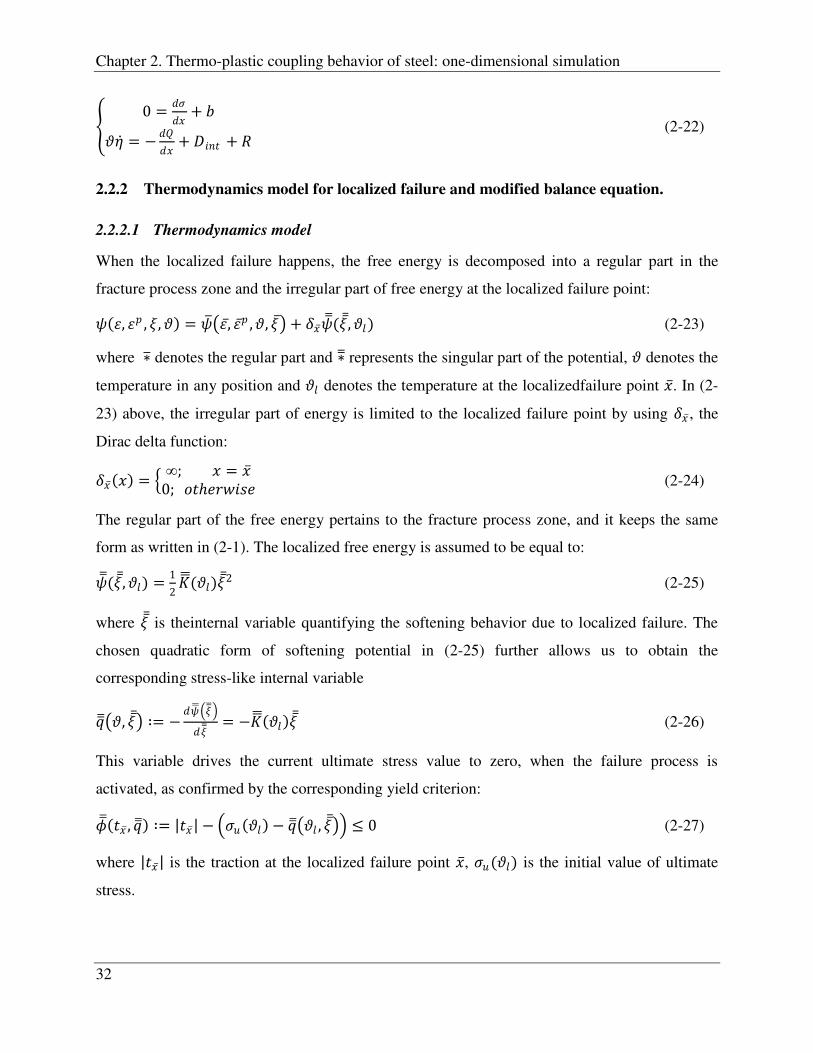
2.2.2 Thermodynamics model for localized failure and modified balance equation.
2.2.2.1 Thermodynamics model
When the localized failure happens, the free energy is decomposed into a regular part in the
fracture process zone and the irregular part of free energy at the localized failure point: , , �, = , , , � + (� , ) (2-23)
where ∗ denotes the regular part and ∗ represents the singular part of the potential, denotes the
temperature in any position and denotes the temperature at the localizedfailure point . In (2-
23) above, the irregular part of energy is limited to the localized failure point by using , the
Dirac delta function:
= ∞; = 0;
(2-24)
The regular part of the free energy pertains to the fracture process zone, and it keeps the same
form as written in (2-1). The localized free energy is assumed to be equal to: (� , ) =1
2 ( )� 2 (2-25)
where � is theinternal variable quantifying the softening behavior due to localized failure. The
chosen quadratic form of softening potential in (2-25) further allows us to obtain the
corresponding stress-like internal variable , � ∶= − � � = − � (2-26)
This variable drives the current ultimate stress value to zero, when the failure process is
activated, as confirmed by the corresponding yield criterion: � , ∶= − � − , � 0 (2-27)
where is the traction at the localized failure point , � ( ) is the initial value of ultimate
stress.

Localized Failure for Coupled Thermo-Mechanics Problems
33
The mechanical properties at localized failure are assumed to have the same dependence on
temperature as the bulk part; hence, we can write: � = � 1 − − 0 (2-28) = [1 − − 0 ] (2-29)
where � and are, respectively, the ultimate stress and softening modulus at reference
temperature 0.
Figure 2-1.Displacement discontinuity at localized failure for the mechanical load
Once the localized failure occurs, the crack opening (further denoted as ( ), seeFigure 2-1)
contributes to a “jump” or irregular part in the displacement field. The total displacement field is
thus sum of regular (smooth) part and irregular part: , = , + ( ) − �( ) (2-30)
where is the Heaviside function introducing the displacement jump
= 0, 1, > (2-31)
In (2-30) above, �( ) is a (smooth) function, introduced to limit the influence of the
displacement jump within the “failure” domain. Usual choice for � in the finite element
implementation pertains to the shape functions of selected interpolation. For example, for a 1D
truss bar with 2 nodes and element length , we can choose: � = 2 = (2-32)
The corresponding illustrations for ( ) and �( ) for a two-node truss-bar element are given
inFigure 2-2
( )
0
Ω 1 Ω 2
Chapter 2. Thermo-plastic coupling behavior of steel: one-dimensional simulation
34
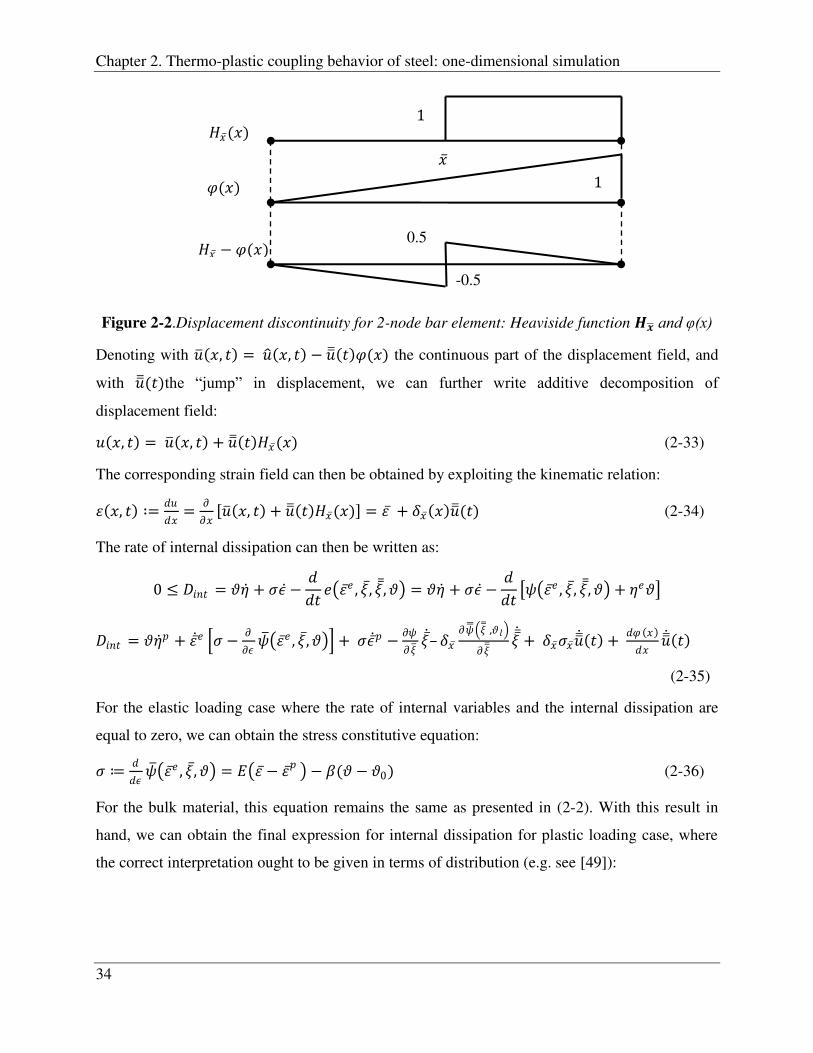
Figure 2-2.Displacement discontinuity for 2-node bar element: Heaviside function � and (x)
Denoting with , = , − �( ) the continuous part of the displacement field, and
with ( )the “jump” in displacement, we can further write additive decomposition of
displacement field: , = , + ( ) (2-33)
The corresponding strain field can then be obtained by exploiting the kinematic relation: , ∶= = , + ( ) = + ( ) (2-34)
The rate of internal dissipation can then be written as:
0 = + � − , � , � , = + � − , � , � , + = + � − , � , + � − � � – � , � � + � +
� (2-35)
For the elastic loading case where the rate of internal variables and the internal dissipation are
equal to zero, we can obtain the stress constitutive equation: � ≔ , � , = − − ( − 0) (2-36)
For the bulk material, this equation remains the same as presented in (2-2). With this result in
hand, we can obtain the final expression for internal dissipation for plastic loading case, where
the correct interpretation ought to be given in terms of distribution (e.g. see [49]):
− �( )
( )
�( )
1
1
0.5
-0.5
Localized Failure for Coupled Thermo-Mechanics Problems
35
Ω = Ω = ( + � + � ) Ω + � | (2-37)
The evolution laws for localized variables are established in the same way as for the classical
continuum model. In particular, the evolution equation for internal variable controlling softening
can be written as:
0 = Ω → � = � = (2-38)
where is the plastic multiplier at the point of localized failure.
2.2.2.2 Thermo-mechanical balance equation
The set of force equilibrium equations consists of two equations:
(1) the local force equilibrium (established for all the bulk domain)
0 =�
+ (2-39)
the stress orthogonality condition to define the traction at localized failure point
0 = + � � Ω (2-40)
(2) Local balance of energy at the localized failure point
For the regular part, the local energy balance is still described by continuum thermodynamic
model (2-21): = − + +
The corresponding state equation (2-3) reads:
= − = − + � 0 → = − + � (2-41)
By considering that = + , = + and = , the local energy
balance can finally be rewritten in the format equivalent to the heat transfer equation: � = − + − − + (2-42)
where the mechanical dissipation and the structural heating (− − ) act as an
additional heat source. This equation holds at any point of the material in the bulk.
We further consider that at the localized failure point, the material has no more ability to store
heat, which implies setting the heat capacity to zero (� = 0). We also take into account that at
localized failure point there is no heat source ( = 0) nor thermal stress ( = 0). Therefore, the
Chapter 2. Thermo-plastic coupling behavior of steel: one-dimensional simulation
36
mechanical dissipation at localized failure can be balanced only against the change of heat flux.
Moreover, the local energy balance equation at the localized failure point ought to be interpreted
in the distribution sense, resulting with the corresponding jump in the heat flux:
0 = − + � → = | (2-43)
where the mechanical dissipation acts as the heat source at the failure point. As indicated
in (2-21) to (2-4γ) above, this results in the corresponding “jump” of the heat flux through the
localized failure section. We note in passing that the jump in the heat flux leads to a change of
the temperature gradient at the localized point. In the finite element implementation, one needs
additional shape functions for describing not only displacement but also temperature field, as
described in the following.
2.3 Embedded-Discontinuity Finite Element Method (ED-FEM) implementation
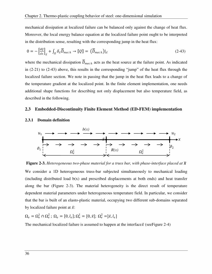
2.3.1 Domain definition
Figure 2-3. Heterogeneous two-phase material for a truss bar, with phase-interface placed at �
We consider a 1D heterogeneous truss-bar subjected simultaneously to mechanical loading
(including distributed load b(x) and prescribed displacements at both ends) and heat transfer
along the bar (Figure 2-3). The material heterogeneity is the direct result of temperature
dependent material parameters under heterogeneous temperature field. In particular, we consider
that the bar is built of an elasto-plastic material, occupying two different sub-domains separated
by localized failure point at : Ω = Ω1 Ω2 ; Ω = 0, ; Ω1 = [0, [; Ω2 =] , ]
The mechanical localized failure is assumed to happen at the interface (seeFigure 2-4)
1
b(x)
R(x)
1
2
2
Ω1 Ω2

Localized Failure for Coupled Thermo-Mechanics Problems
37
In the following, the indices “1” is used for all the thermodynamics variables relate to sub-
domain Ω1 , and the indices “β” to the second sub-domain Ω2.
2.3.2 „Adiabatic‟ operator splitting solution procedure
Due to the positive experience of Kassiotis et al. (see [50]), we choose the operator split method
based upon adiabatic split to solve this problem. In the most general case with active localized
failure, the coupled thermomechanical problem is described by a set of mechanical balance
equations defined in (2-39) and (2-40), accompanied by the energy balance equations in (2-42)
and (2-43). Solving all of these equations simultaneously is certainly not the most efficient
option. In order to increase the solution efficiency, we can choose between two possible operator
split implementations: isothermal and adiabatic (see [17]). We note in passing that the isothermal
operator split is not capable of providing the stability of the computation (see [50]). Therefore,
we focus only upon the adiabatic operator split method. In this method, the problem is divided
into two phases, with each one contribution to change of temperature:
Phase 1 - Mechanical part
with “adiabatic”condition Phase 2- Thermal part
0 =�
+ = 0 → � = − − (at localized failure point): �1| = �2| =
� = − + = | The computations of the mechanical and thermal states remain coupled through the adiabatic
condition.
0
( )
( )
� �
Figure 2-4.Two sub-domain � and � separated by localized failure point at �
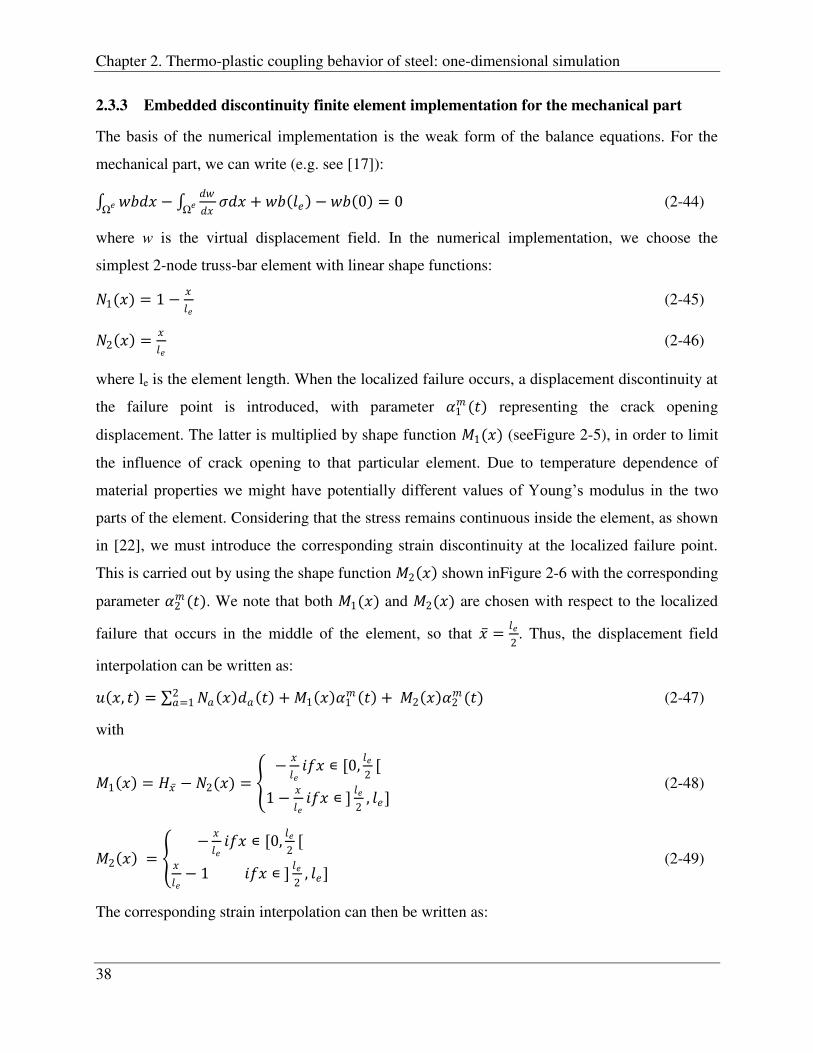
Chapter 2. Thermo-plastic coupling behavior of steel: one-dimensional simulation
38
2.3.3 Embedded discontinuity finite element implementation for the mechanical part
The basis of the numerical implementation is the weak form of the balance equations. For the
mechanical part, we can write (e.g. see [17]):
Ω − � + − 0 = 0Ω (2-44)
where w is the virtual displacement field. In the numerical implementation, we choose the
simplest 2-node truss-bar element with linear shape functions:
1( ) = 1 − (2-45)
2 = (2-46)
where le is the element length. When the localized failure occurs, a displacement discontinuity at
the failure point is introduced, with parameter 1 ( ) representing the crack opening
displacement. The latter is multiplied by shape function 1( ) (seeFigure 2-5), in order to limit
the influence of crack opening to that particular element. Due to temperature dependence of
material properties we might have potentially different values of Young‟s modulus in the two
parts of the element. Considering that the stress remains continuous inside the element, as shown
in [22], we must introduce the corresponding strain discontinuity at the localized failure point.
This is carried out by using the shape function 2 shown inFigure 2-6 with the corresponding
parameter 2 ( ). We note that both 1( ) and 2( ) are chosen with respect to the localized
failure that occurs in the middle of the element, so that =2
. Thus, the displacement field
interpolation can be written as: , = 2=1 + 1 1 + 2 2 ( ) (2-47)
with
1 = − 2( ) = − ∊ [0,2
[
1 − ∊ ]2
, ]
(2-48)
2 = − ∊ [0,2
[− 1 ∊ ]2
, ]
(2-49)
The corresponding strain interpolation can then be written as:

Localized Failure for Coupled Thermo-Mechanics Problems
39
, = ,
= 2=1 + 1 1 + 2 2 ( )
(2-50)
1 = 1 = − 1
∊ [0,2
2, ]− 1
+ = =2
= 1 + ( =
2) ; 1 = − 1
(2-51)
2 = 2 = − 1 ∊ [0,
2[
1 ∊ ]2
, ]
(2-52)
1
-0.5
� ( )
( )
= 0 = =
− 1
M1(x)
x = le
− x le
G1(x) Ł0
x = 0 x = x 1 − x
le
x
−1
le
Figure 2-5Displacement discontinuity shape function M1(x) and its derivative.
Figure 2-6. Strain discontinuity shape function M2 and its derivative

Chapter 2. Thermo-plastic coupling behavior of steel: one-dimensional simulation
40
The corresponding discrete approximation of the virtual displacement and strain can be written
in an equivalent form: = + 1 1 + 2 2 (2-53) = + 1
( ) 1 + 2 2 (2-54)
where 1 and 2 are the variations corresponding to 1 ( ) and 2 ( ), respectively.With these
interpolations in hand, the weak form of the equilibrium equation can be recast in incompatible
mode format (see [18]) as the set of equations:
=1( , − , ) = 0; , = � , 1 , 2 , �
1 = 0; 1 = 1� , 1 , 2 , Ω + 1 , 2
2 = 0; 2 = 2� , 1 , 2 , Ω (2-55)
Given highly nonlinear material behavior, this set of equations ought to be solved by an iterative
scheme. If ζewton‟s method is used, we make systematic use of the consistent linearization (see
[17]), where the corresponding incremental stress-strain relation has to be obtained. We note that
the chosen isoparametric elements provide continuum consistent interpolation, and furthermore
that the continuum and discrete tangent modulus remain the same in one-dimensional setting (see
[17]). Thus, we start with the consistent linearization of the continuum problem to obtain the
stress rate constitutive equation, one in each sub-domain „i‟: � = − − (2-56)
The time derivative of temperature can be computed by imposing the adiabatic step: = − + � = 0 → = − � − (2-57)
Combining the last two results, we finally obtain � =, − ; ,
= +2� (2-58)
Where , denotes the adiabatic tangent modulus. For sub-domain i, undergoing elastic
loading, with = 0, the constitutive equation can be simplified as: � =, (2-59)
On the other hand, if sub-domain i undergoes plastic loading, the consistency condition requires:
Localized Failure for Coupled Thermo-Mechanics Problems
41
� � , , = �� � +
�� � +� = 0 (2-60)
With the expression for � chosen herein, (2-60) can further be simplified to: � � − � + � + � = 0 (2-61)
By using equation (2-57), we get the constitutive equation in rate form: � = � � + � � + − � � + � � (2-62)
From equation (2-58), we have = − � , (2-63)
Combining equations(2-62) and (2-63) we can establish the constitutive equation for a plastic
domain “i”μ � = � � + � � + − � � + � � ( − � ,
)
� =,
,+ − � � + � �
,
(2-64)
In conclusion, the following constitutive equation can be employed:
� = ; = , ; � < 0
, ; � = 0
(2-65)
where , and , are defined in (2-59) and (2-64), respectively.
To solve the problem, two operator split are employed (e.g. see[17]) with „local‟ and „global‟
phases of computation. The former provides the internal variables, while the latter gives the
nodal values of displacement. We briefly describe those two algorithm phases:
i) Local computation:
Given: , +1, , , � , , 1, , � , 2,
Find: , +1, � , +1, , +1, � +1, 2, +1
which should obey the following conditions:

Chapter 2. Thermo-plastic coupling behavior of steel: one-dimensional simulation
42
� � , +1, , +1 0; , +1 0 , +1� , +1 = 0; = 1,2 (2-66)
� +1, +1 0; +1 0 +1� +1 = 0
(2-67)
and
2 �1( , +1, 1, 2)Ω1+ 2 �2 , +1, 1, 2 Ω2
= 0 (2-68)
We note that (2-66) is used to compute plastic internal variables of two sub-domains at the step
(n+1) from the previous step (n) by the so-called „return-mapping‟ algorithm (see [51]).
Conditions (2-67) and (2-68) are used to compute 1, +1 and 2, +1 by using the following
algorithm:
i) Assume 1, +1 ≔ 1, , 2, +1 = 0
ii) Compute trial stress at the two sub-domains with 1, +1 and 2, +1
+1 , = ,
= + 1 1,
, + 2 2, +1,
( ) � , +1 , +1, 1, +1, 2, +1 = ( +1 − ) iii) Compute trial value of tension force at localized failure point
+1 = − 1� , +1, 1, +1, 2, +1 Ω (2-69)
IF � +1 , +1 0 THEN 1, +1 ≔ 1, and go to step (vi)
iv) IF � +1 , +1 > 0 THEN +1 =� +1 , +1
1 + 22
+ (2-70)
(le is the length of the element) � +1 = � + +1 (2-71)
1, +1 = 1, + +1 +1 (2-72)
Return to step (ii) with the updated value of 1, +1 and � +1
v) Compute updated value of 2, +1 from condition (1-69)

Localized Failure for Coupled Thermo-Mechanics Problems
43
2, +1 ≔ �1 −�2 1 + 2
(2-73)
With the updated value of 2, +1 check
IF 2 � ( , +1, 1 , 2 )Ω = 0 THEN
EXIT
ELSE
Return to step (ii)
ii) Global computation
In global computation phase, the system (2-55) is rewritten in linearized form:
0
0
0
2
1
,int,
1
e
e
eextenel
e
Lin
Lin
Lin A
h
h
ff
(2-74)
The corresponding result of consistent linearization can be recast in matrix notation:
� � ��� � + 1
1
��� �� � �� 1� 2
= +1, − +1
,
0
0
(2-75)
where we have:

Chapter 2. Thermo-plastic coupling behavior of steel: one-dimensional simulation
44
1 = � ( )Ω ; 1 = 1 + 2
2 1 −1−1 1
(2-76)
1 = � 1( )Ω ; 1 = 1 + 2
2 1−1
(2-77)
2 = � 2( )Ω ; 2 = 1 − 2
2 1−1
(2-78)
1 = 1( )
1( )Ω ; 1 = 1 + 2
2 (2-79)
2 = 1 2( )Ω ; 2 = 1 − 2
2 (2-80)
= 2( ) 2( )Ω ; = 1 + 2
2 (2-81)
∂t α1m ∂α1
m = K sign(tx ) (2-82)
By using static condensation at the converged value of incompatible mode parameters, � � is
obtained as the solution of: � � � = +1, − +1
, (2-83)
where takes the standard form for the stiffness matrix:
= 1 + 2
2− ( 1 + 2 ) 1 2
2 3 + 1 − 2 2
4 2
1 22 +
1 + 2 2
1 −1−1 1 (2-84)
Once Δ � is obtained from (1-83), the nodal displacement can be updated: �,�+ = �,� + � �.
2.3.4 Embedded discontinuity finite element implementation for the thermal part
In thermal part, the heat transfer equation is written for two sub-domains as the following: � = − + (2-85)
And at the localized failure zone, the heat propagation happens with a jump in heat flux: � = � � |� (2-86)
In each of two sub-domains, the heat transfer obeys the Fourier heat conduction law:
= − (2-87)
The local energy balance can be rewritten in the equivalent form to the heat equation:

Localized Failure for Coupled Thermo-Mechanics Problems
45
� =2
2+ (2-88)
The strong form (2-85) is further transferred into weak form by introducing an arbitrary
temperature field, denoted as , and by applying the virtual work laws: � − 2
2− = 0
0 (2-89)
After integration by part, we can finally obtain the following weak form: � + =000
(2-90)
We consider a 2-node truss-bar element. The nodal values of temperature and the weighting
temperature at node i are denoted as dϑi and wi, respectively. dand w denote the real and the
arbitrary nodal temperature vector, respectively. For a 2-node element, we have:
� = 1
2
;� = 1
2 ,
The real and weighting temperature fields along the element are constructed with
interpolation shape functions. Furthermore, the jump of temperature gradient at the localized
failure point, is represented by an additional shape function: = ( )2=1 + 2 2( ) (2-91)
where ( ) and 2( ) are defined in (2-49) and illustrated in Figure 2-6 for a two-node truss-
bar element, whereas 2( ) is the variable controlling the „jump‟ in temperature gradient. We
note that ( ) =1
2 1 ( ) + 2 + 2( ), where is the temperature at the interface (at the
middle of the element).
Apply the Fourier laws to the localized point, we have:
= − 2
2 = − 2
2 +
22
2 2 = − 2

Chapter 2. Thermo-plastic coupling behavior of steel: one-dimensional simulation
46
→ = − 2 (2-92)
where denotes the heat conductivity coefficient at the localized failure. By combining
equation (2-92) with equation (2-86), we can infer the equation for 2( ): = − 2 = → 2 = (2-93)
The iso-parametric interpolation functions are used for the weighting temperature field: = (2-94)
By taking into account the interpolation of real and weight temperature fields, the weak form (2-
90) is finally reduced to: � + � 2 2 + +Ω 2 2 = (2-95)
Finally, the finite element equations to be solved for the “thermal” phase are given byμ
=1 � � + 2 + � � + � 2 = =1 � (2-96)
where �2 2 = � � ; �2 2 =24 7�1 1 + �2 2 2(�1 1 + �2 2)
2(�1 1 + �2 2) �1 1 + 7�2 2 (2-97)
1 2 = � 2 � ; 1 2 = −24 2�1 1 + �2 2�1 1 + 2�2 2
(2-98)
�2 2 = � ;�2 2 = 1+ 2
2 1 −1−1 1
(2-99)
�1 2 = 2 � ;�1 2 = 1− 2
2 1−1
(2-100)
11 2
= ; 11 2
=8 3 1 + 2
1 + 3 2 (2-101)
There are many methods capable of solving the time-dependent equation (2-96) (see [17]). In
this paper, the Newmark integration scheme is chosen. Assuming that the heat transfer problem
lasts for a duration [0,T], this duration can be divided into n increments: [t0=0, t1.., tk, ..tn-1, tn =T]
with the time step h = tk+1 – tk.
By considering the equation of Newmark: Δ ϑ = Δ =hΔ ϑ (where and are the
Newmark coefficients) and by linearization, equation (2-96) becomes:
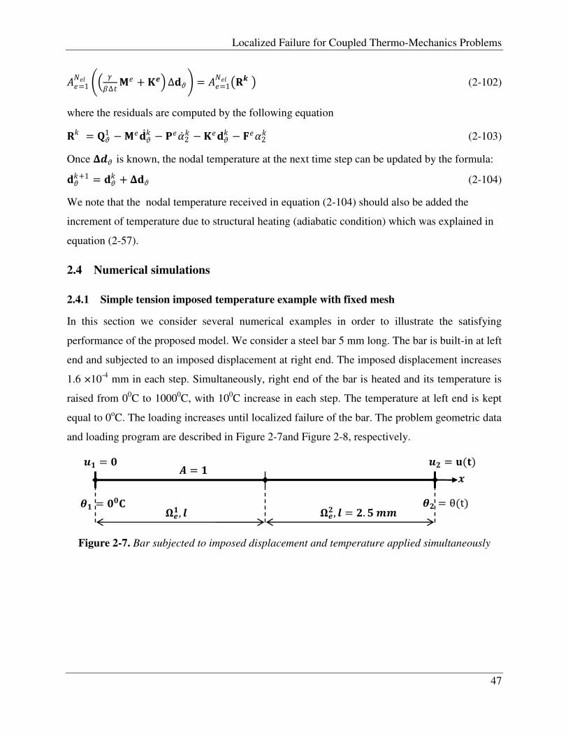
Localized Failure for Coupled Thermo-Mechanics Problems
47
=1 Δ � + � Δ = =1 � (2-102)
where the residuals are computed by the following equation � = 1 −� − 2 −� − � 2 (2-103)
Once � is known, the nodal temperature at the next time step can be updated by the formula:
+1 = + � (2-104)
We note that the nodal temperature received in equation (2-104) should also be added the
increment of temperature due to structural heating (adiabatic condition) which was explained in
equation (2-57).
2.4 Numerical simulations
2.4.1 Simple tension imposed temperature example with fixed mesh
In this section we consider several numerical examples in order to illustrate the satisfying
performance of the proposed model. We consider a steel bar 5 mm long. The bar is built-in at left
end and subjected to an imposed displacement at right end. The imposed displacement increases
1.6 ×10⁻⁴ mm in each step. Simultaneously, right end of the bar is heated and its temperature is
raised from 00C to 10000C, with 100C increase in each step. The temperature at left end is kept
equal to 0oC. The loading increases until localized failure of the bar. The problem geometric data
and loading program are described in Figure 2-7and Figure 2-8, respectively.
Figure 2-7. Bar subjected to imposed displacement and temperature applied simultaneously
=
� = � � = θ(t)
= ( ) �
� ,
= .�
� , = .�
� =
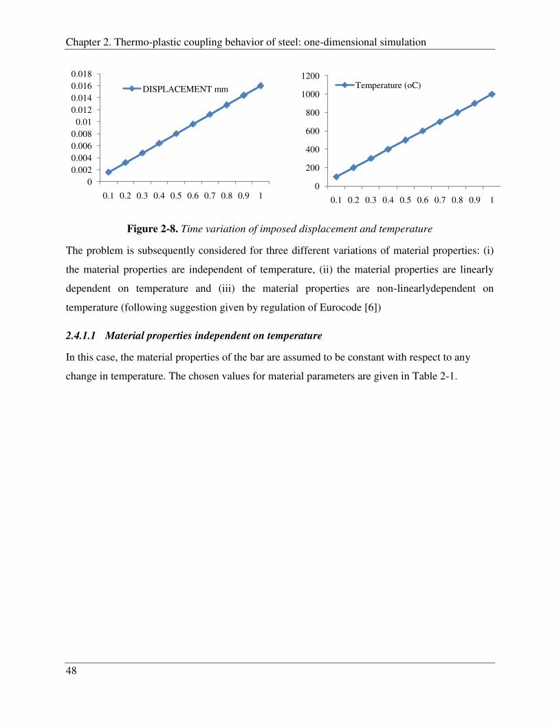
Chapter 2. Thermo-plastic coupling behavior of steel: one-dimensional simulation
48
Figure 2-8. Time variation of imposed displacement and temperature
The problem is subsequently considered for three different variations of material properties: (i)
the material properties are independent of temperature, (ii) the material properties are linearly
dependent on temperature and (iii) the material properties are non-linearlydependent on
temperature (following suggestion given by regulation of Eurocode [6])
2.4.1.1 Material properties independent on temperature
In this case, the material properties of the bar are assumed to be constant with respect to any
change in temperature. The chosen values for material parameters are given in Table 2-1.
00.0020.0040.0060.008
0.010.0120.0140.0160.018
0.1 0.2 0.3 0.4 0.5 0.6 0.7 0.8 0.9 1
DISPLACEMENT mm
0
200
400
600
800
1000
1200
0.1 0.2 0.3 0.4 0.5 0.6 0.7 0.8 0.9 1
Temperature (oC)

Localized Failure for Coupled Thermo-Mechanics Problems
49
Table 2-1. Material properties of steel bar
Material Properties Value Dimension
Young modulus (E) 205000 MPa
Initial yield stress (� ) 250 MPa
Ultimate stress (� ) 300 MPa
Plastic hardening modulus (Kp) 20000 MPa
Localized softening modulus (K ) -30000 MPam-1
Mass Density (�) 7.865 10-9 Ns2mm-4
Thermal conductivity (k) 45 N s-1K-1
Heat specific (c) 0.46 109 mm2s-2K-1
Thermal elongation( ) 0.00001
The computed results for stress-strain curves in two sub-domains are presented in Figure 2-9,
while the force-displacement curve of the bar is given in Figure 2-10. In Table 2-2 and Figure
2-11, we show the resulting time evolution of temperature and its distribution along the bar. For
this case with material properties independent on temperature, we can conclude that there is no
difference in the strain values between two sub-domains. The „jump‟ in temperature gradient
( ), which appears at localized failure point, also remains very small. The computed
dissipation due to plasticity in fracture process zone is 36.63Nmm, while the dissipation due to
localized failure is 29.44Nmm. In summary, the total mechanical dissipation in the bar is equal to
66.07Nmm.
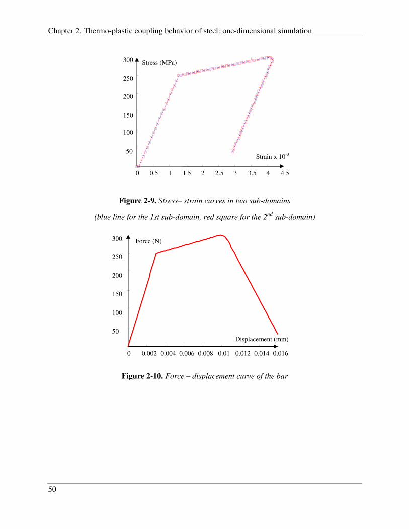
Chapter 2. Thermo-plastic coupling behavior of steel: one-dimensional simulation
50
Figure 2-9. Stress– strain curves in two sub-domains
(blue line for the 1st sub-domain, red square for the 2nd
sub-domain)
Figure 2-10. Force – displacement curve of the bar
0 0.002 0.004 0.006 0.008 0.01 0.012 0.014 0.016
50
100
150
200
250
300
Displacement (mm)
Force (N)
0 0.5 1 1.5 2 2.5 3 3.5 4 4.5
Strain x 10-3 50
100
150
200
250
300
Stress (MPa)

Localized Failure for Coupled Thermo-Mechanics Problems
51
Table 2-2.Time Evolution of Temperature along the Bar
Time
at
x =0
at
x=0.25le
at
x = 0.5le
at
x=0.75le
at
x = le Δ
0 0.0000 0.0000 0.0000 0.0000 0.0000 0.0000
0.1 0.0000 25.0000 50.0000 75.0000 100.0000 0.0000
0.2 0.0000 50.0000 100.0000 150.0000 200.0000 0.0000
0.3 0.0000 75.0000 150.0000 225.0000 300.0000 0.0000
0.4 0.0000 100.0000 200.0000 300.0000 400.0000 0.0000
0.5 0.0000 125.0000 250.0000 375.0000 500.0000 0.0000
0.6 0.0000 150.0000 300.0000 450.0000 600.0000 0.0000
0.7 0.0000 175.0005 350.0010 525.0005 700.0000 0.0010
0.8 0.0000 200.0007 400.0014 600.0007 800.0000 0.0014
0.9 0.0000 225.0008 450.0015 675.0008 900.0000 0.0015
1 0.0000 250.0008 500.0016 750.0008 1000.000 0.0016
where � = =0.5 − 0.5( =0 + = )
Figure 2-11. Distribution of temperature (oC) along the bar at chosen values of time
0
100
200
300
400
500
600
700
0 0.25 0.5 0.75 1
Tem
per
atu
re (
oC
)
x/l
t=0.2 s
t=0.4 s
t=0.6 s
t=0.8 s
t=1 s

Chapter 2. Thermo-plastic coupling behavior of steel: one-dimensional simulation
52
Figure 2-12. Evolution of Δ � versus time (in 0C)
2.4.1.2 Material properties are linearly dependent on temperature
In this example, the mechanical material properties of the steel bar chosen in the first example
(see Table 2-1) are assumed to hold only at reference temperature (equal to 00C). For other
temperature values, they vary linearly according to the following expression:
initial yield stress: � ( ) = 250 1 − 0.001 MPa
ultimate strength: � = 300 1 − 0.0015
Young‟s modulusμ ( ) = 2.05 × 10⁵ 1 − 0.0008
plastic hardening modulus: ( ) = 2 × 10⁴ 1 − 0.0008
localized softening modulus: = −3 × 10⁴ 1 − 0.0008 a
The thermal material properties are independent on temperature and equal to those in the first
example. The resulting stress-strain curves in two sub-domains and resulting force-displacement
diagram are presented in Figure 2-13 and Figure 2-14, respectively.
0C
t(s)
0.0010
0.00140.0015
0.0016
0
0.0002
0.0004
0.0006
0.0008
0.001
0.0012
0.0014
0.0016
0.0018
0 0.1 0.2 0.3 0.4 0.5 0.6 0.7 0.8 0.9 1
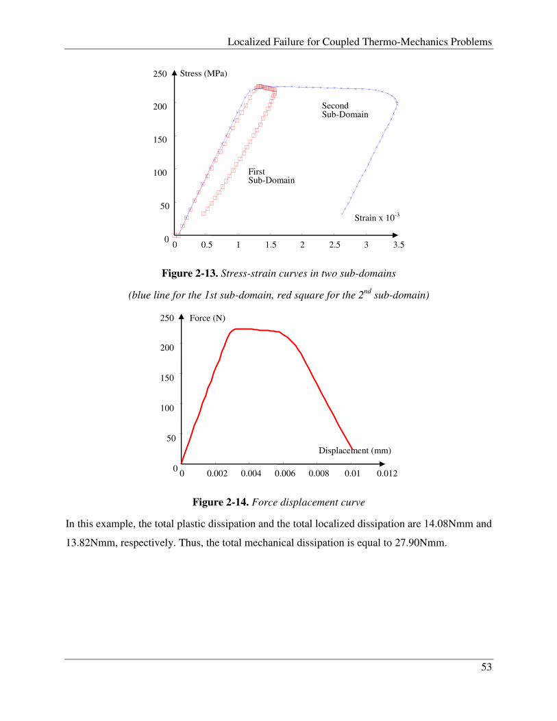
Localized Failure for Coupled Thermo-Mechanics Problems
53
Figure 2-13. Stress-strain curves in two sub-domains
(blue line for the 1st sub-domain, red square for the 2nd
sub-domain)
Figure 2-14. Force displacement curve
In this example, the total plastic dissipation and the total localized dissipation are 14.08Nmm and
13.82Nmm, respectively. Thus, the total mechanical dissipation is equal to 27.90Nmm.
0 0.002 0.004 0.006 0.008 0.01 0.012 0
50
100
150
200
250
Displacement (mm)
Force (N)
0 0.5 1 1.5 2 2.5 3 3.5 0
50
100
150
200
250
Strain x 10-3
Stress (MPa)
Second Sub-Domain
First Sub-Domain

Chapter 2. Thermo-plastic coupling behavior of steel: one-dimensional simulation
54
Table 2-3.Time evolution of temperature along the bar
Time
at
x =0
at
x=0.25le
at
x = 0.5le
at
x=0.75le
at
x = le Δϑ
0.0000 0.0000 0.0000 0.0000 0.0000 0.0000 0.0000
0.1000 0.0000 25.0000 50.0000 75.0000 100.0000 0.0000
0.2000 0.0000 50.0000 100.0000 150.0000 200.0000 0.0000
0.3000 0.0000 75.0000 150.0000 225.0000 300.0000 0.0000
0.3500 0.0000 87.5000 175.0000 262.5000 350.0000 0.0000
0.4000 0.0000 100.0000 199.9999 300.0000 400.0000 -0.0001
0.4500 0.0000 112.5002 225.0005 337.5002 450.0000 0.0005
0.5000 0.0000 125.0004 250.0007 375.0004 500.0000 0.0007
0.5500 0.0000 137.5004 275.0008 412.5004 550.0000 0.0008
0.6000 0.0000 150.0004 300.0008 450.0004 600.0000 0.0008
0.6300 0.0000 157.5004 315.0008 472.5004 630.0000 0.0008
where � = =0.5 − 0.5( =0 + = )
Figure 2-15. Evolution of temperature (oC) along the bar in time
0
100
200
300
400
500
600
700
0 0.25 0.5 0.75 1
Tem
pre
ratu
re (
0C
)
x/le
t=0.2 s
t=0.35 s
t=0.45 s
t=0.55 s
t=63 s

Localized Failure for Coupled Thermo-Mechanics Problems
55
Figure 2-16. Evolution of Δϑ versus time (in 0C)
From the results presented in the figures above, we can conclude that the temperature variations
deeply influence the behavior of the bar. In particular, the displacement at the end of the bar
when failure occurs reduces from 0.016mm to 0.011mm, the initial yield stress falls down to
approximately 225MPa from 250MPa and so the ultimate strength reduces from 300MPa to
about 220MPa. The total dissipation in this example is also reduced, from 66.07Nmm to
27.90Nmm. Figure 2-13indicates that the variation of temperature field leads to a significant
difference in the material behavior and computed stress-strain curves in two parts of the bar. The
“jump” in temperature gradient accompanying localized failure remains relatively small.
2.4.1.3 Material properties non-linearly dependent on temperature (Eurocode 1993-1-2 [6])
In Eurocode1993-1-2 (see[6]), the material properties of steel bar subjected to thermal loading
are not constant but dependent on temperature as multi-linear functions. Based on those
regulations, evolution of mechanical properties as functions of temperature can be established as
follows:
initial yield stress: � ( ) = 250 1 − � − 20 MPa
ultimate strength: � = 300 1 − � − 20 MPa
Young‟s modulusμ ( ) = 2.05 × 10⁵ 1 − − 20 MPa
plastic hardening modulus: ( ) = 2 × 10⁴ 1 − − 20 MPa
localized softening modulus: = −3 × 10⁴ 1 − − 20 Pa
oC
t(s)
0.0007
0.0008
-0.0002
0
0.0002
0.0004
0.0006
0.0008
0.001
0 0.1 0.2 0.3 0.35 0.4 0.45 0.5 0.55 0.6 0.63
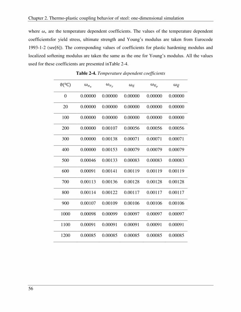
Chapter 2. Thermo-plastic coupling behavior of steel: one-dimensional simulation
56
where ∗ are the temperature dependent coefficients. The values of the temperature dependent
coefficientsfor yield stress, ultimate strength and Young‟s modulus are taken from Eurocode
1993-1-2 (see[6]). The corresponding values of coefficients for plastic hardening modulus and
localized softening modulus are taken the same as the one for Young‟s modulus. All the values
used for these coefficients are presented inTable 2-4.
Table 2-4. Temperature dependent coefficients ϑ(0C) ω� ω� ω ω ω
0 0.00000 0.00000 0.00000 0.00000 0.00000
20 0.00000 0.00000 0.00000 0.00000 0.00000
100 0.00000 0.00000 0.00000 0.00000 0.00000
200 0.00000 0.00107 0.00056 0.00056 0.00056
300 0.00000 0.00138 0.00071 0.00071 0.00071
400 0.00000 0.00153 0.00079 0.00079 0.00079
500 0.00046 0.00133 0.00083 0.00083 0.00083
600 0.00091 0.00141 0.00119 0.00119 0.00119
700 0.00113 0.00136 0.00128 0.00128 0.00128
800 0.00114 0.00122 0.00117 0.00117 0.00117
900 0.00107 0.00109 0.00106 0.00106 0.00106
1000 0.00098 0.00099 0.00097 0.00097 0.00097
1100 0.00091 0.00091 0.00091 0.00091 0.00091
1200 0.00085 0.00085 0.00085 0.00085 0.00085

Localized Failure for Coupled Thermo-Mechanics Problems
57
Figure 2-17.Temperature dependent coefficients (according to [6])
The evolution of thermal properties is also taken from Eurocode1993-1-2.
Thermal elongation
= 1.2 × 10⁻⁵ + 0.4 × 10⁻⁸ 2 − 2.416 × 10⁻⁴, 200 < 7500
1.1 × 10⁻² , 7500 < 8600
2 × 10⁻⁵ − 6.2 × 10⁻³, 8600 < 12000
Specific heat
=
425 + 7.73 × 10⁻¹ − 1.69 × 10⁻³ 2 + 2.22 × 10⁻⁶ 3 200 < 6000
666 +13002
738 − 6000 < 7350
545 +17820− 731
7350 < 9000
650 9000
Thermal conductivity
= 54 − 3.33 × 10⁻²�
, 200 < 8000
27.3�
, 8000 12000
The main results obtained considering those evolutions are described subsequently in terms of
the stress-strain curves, force-displacement diagram and corresponding temperature variations.
0.00000
0.00050
0.00100
0.00150
0.00200
20 100 200 300 400 500 600 700 800 900 1000 1100 1200
ϑωбu
ωбy
ωE = ωK
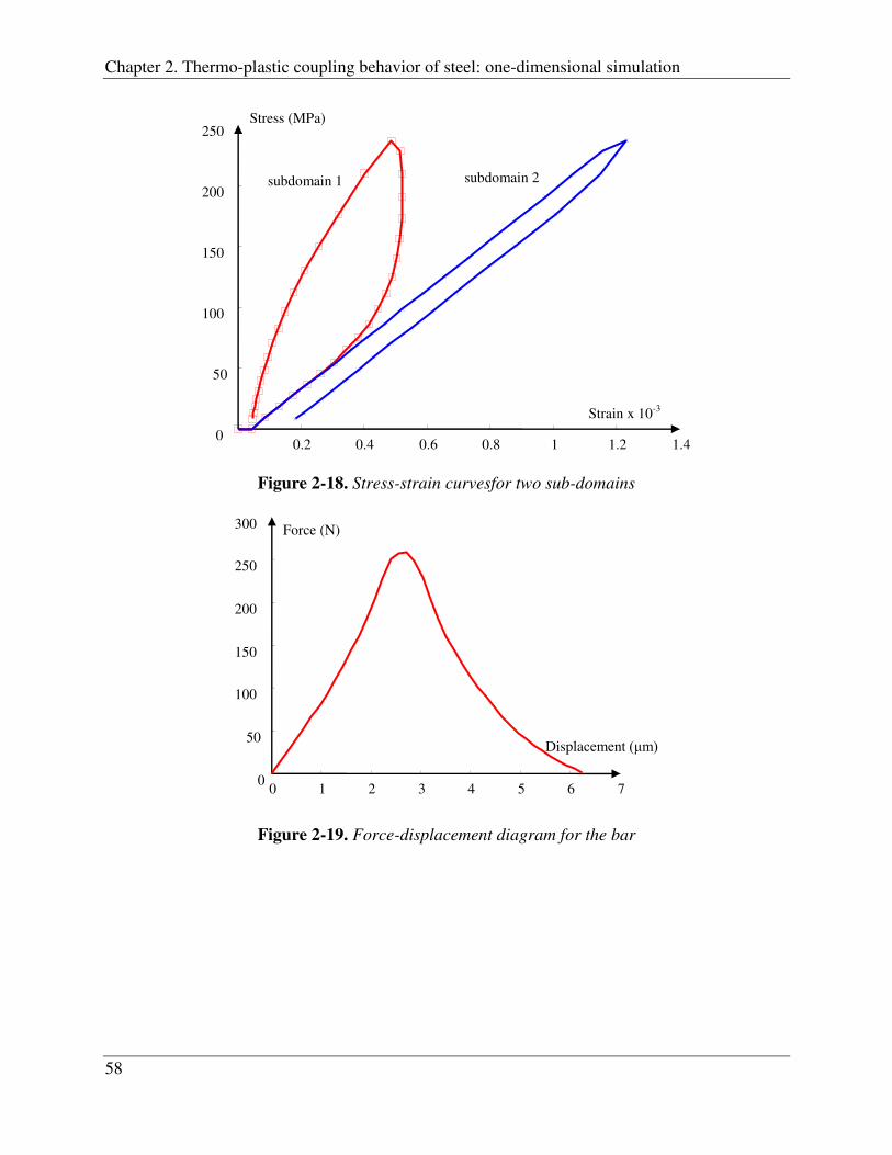
Chapter 2. Thermo-plastic coupling behavior of steel: one-dimensional simulation
58
Fig.17 Stress-strain curvesfor two sub-domains (
Figure 2-19. Force-displacement diagram for the bar
0 1 2 3 4 5 6 7 0
50
100
150
200
250
300
Displacement ( m)
Force (N)
0.2 0.4 0.6 0.8 1 1.2 1.4 0
50
100
150
200
250
subdomain 1
Stress (MPa)
Strain x 10-3
subdomain 2
Figure 2-18. Stress-strain curvesfor two sub-domains

Localized Failure for Coupled Thermo-Mechanics Problems
59
Table 2-5. Distribution of temperature along the bar
Time
at
x =0
at
x=0.25le
at
x = 0.5le
at
x=0.75le
at
x = le Δ
0.0000 0.0000 0.0000 0.0000 0.0000 0.0000 0.0000
0.0500 0.0000 12.5000 25.0000 37.5000 50.0000 0.0000
0.1000 0.0000 25.0000 50.0000 75.0000 100.0000 0.0000
0.1500 0.0000 37.5000 75.0000 112.5000 150.0000 0.0000
0.2000 0.0000 49.9998 99.9996 149.9998 200.0000 -0.0004
0.2500 0.0000 62.5020 125.0041 187.5020 250.0000 0.0041
0.3000 0.0000 75.0053 150.0106 225.0053 300.0000 0.0106
0.3500 0.0000 87.5094 175.0188 262.5094 350.0000 0.0188
0.3900 0.0000 97.5133 195.0265 292.5133 390.0000 0.0265
where � = =0.5 − 0.5( =0 + = )
Figure 2-20. Distribution of temperature (0C) along the bar due to time
0
50
100
150
200
250
300
350
400
450
0 0.25 0.5 0.75 1
Tem
per
atu
re (
0C
)
x/le
t=0.1 s
t=0.2 s
t=0.3 s
t=0.39 s

Chapter 2. Thermo-plastic coupling behavior of steel: one-dimensional simulation
60
Figure 2-21. Evolution of Δϑ vs time
where � = =0.5 − 0.5( =0 + = )
Figure 2-18 clearly shows the large difference in strain between the two sub-domains, both
before and after the initiation of localized failure. Mathematically, this difference is due to
different values of 1 and 2 (see (2-51)). Before the initiation of localized failure, the
difference in temperature will lead to a difference in tangent modulus between two sub-domains,
which results in the appearence of 2 which represents the difference in strain between the two
sub-domains. After localized failure occurs, 1 increases and contributes to the different
behaviors in the two parts of the bar.
From Table 2-5 and Figure 2-20, we can see that the temperature distribution is nonlinear. Its
gradient changes at the middle of the bar. This change can be computed through 2 (see equation
(2-92)). It is noted that the magnitude of 2 increases and then decreases with time (see Table
2-5and Figure 2-20). However, Figure 2-20also shows that the change in temperature gradient is
relatively small in comparison with the temperature at the localized failure point (the maximum
ratio of Δ
( is the temperature of the localized point) is approximately 0.0136%.), and
therefore does not significantly contribute to the final results.
In this example, once again, we observe a reduction in the strength of the bar: the maximum
displacement that can be applied to the bar now reduces to roughly 0.006 mm from 0.010 mm
and 0.016 mm in the second and the first example, respectively.
The total mechanical dissipation along the bar is significantly smaller than the second and the
first example (15.01Nmm in comparison to 27.90Nmm and 66.07Nmm). The major contribution
0C
t(s)
0.0188
0.0265
-0.005
0
0.005
0.01
0.015
0.02
0.025
0.03
0 0.05 0.1 0.15 0.2 0.25 0.3 0.35 0.39

Localized Failure for Coupled Thermo-Mechanics Problems
61
comes from the localized dissipation: 10.55 Nm in comparison with the total plastic dissipation:
4.47Nm.
2.4.2 Mesh refinement, convergence and mesh objectivity
In this example, we study the influence of the chosen number of elements upon the computed
final results. The geometry description is given in Figure 2-22.
We consider a steel bar built-in at left end and subjected to an imposed displacement at right end
(increasing linearly to 2mm). Simultaneously, right end of the bar is heated and its temperature is
raised from 00C to 1000C. The temperature of left end is kept constant and equal to 0oC. The
material properties of the bar are considered as temperature independent and shown in Table 2-6.
Table 2-6. Material properties
Material Properties Value Dimension
Young modulus (E) 205000 MPa
Initial yield stress (� ) 250 MPa
Ultimate stress (� ) 300 MPa
Plastic hardening modulus (Kp) 20000 MPa
Localized softening modulus (K ) -45 MPam-1
Mass Density (�) 7.865 10-9 Ns2mm-4
Thermal conductivity (k) 45 N s-1K-1
Heat specific (c) 0.46 109 mm2s-2K-1
Thermal elongation( ) 0.00001
u1 = 0
ϑ1 = 00C ϑ2 = ϑ(t)
u2 = u(t) �
l = 1m
A = 1 n elements
Figure 2-22.Bar subjected to imposed loading and imposed temperature

Chapter 2. Thermo-plastic coupling behavior of steel: one-dimensional simulation
62
The results are again illustrated by using several figures. In particular, Figure 2-23shows the load
– displacement diagram of the bar computed by using 3, 5, 7 and 9 elements. It is noted that the
computed curve after localized failure is not dependent on the chosen mesh (see Figure
2-23).This result proves the convergence of the numerical solution with respect to mesh
refinement (see[17]).
2.4.3 Heating effect of mechanical loading
In this example, we would like to illustrate the heating effect produced by mechanical dissipation
in a bar when localized failure occurs. Consider a steel bar of 10mm long, fixed at left end and
subjected to an increasing displacement (0.045mm/s) at right end until collapse. The initial
temperature is constant along the bar and equal to 00C. Material properties of the bar are given
inTable 2-1. Due to a problem in manufacturing, the ultimate stress at the middle point reduces
to 299MPa instead of 300MPa in other part (see Figure 2-24).
Figure 2-23. Load-displacement diagram with different number of elements
0 0.2 0.4 0.6 0.8 1 1.2 1.4 1.6 1.8 2
50
100
150
200
250
300
- 5 elements
Force (N)
Displacement (mm)
+ 7 elements
* 9 elements

Localized Failure for Coupled Thermo-Mechanics Problems
63
The problem is solved with two different meshes: 5 elements and 9 elements. In these two
meshes, the middle element represents the zone with smaller ultimate stress (� = 299 ).
The localized failure will therefore occur in this element. The computed load-displacement
diagram of the bar is given in FigureFigure 2-25, while the evolution of temperature in the bar is
shown inFigure 2-26 and Figure 2-27.
Figure 2-25. Load-displacement curve
The computed results clearly show the heating effect produced by the mechanical dissipation.
Namely, the plastic dissipation equals heat supply leading to temperature increase. Initially, the
dissipation in FPZ is equally distributed along the bar so that the temperature at every part of the
bar remains the same. However, with the start of localized failure, additional dissipation at
0 0.005 0.01 0.015 0.02 0.025 0.03 0.035 0.04 0.045 0
50
100
150
200
250
300
Displacement (mm)
Force (N)
1 middle element
1 = 0
= 00C
2 = u(t) �
= 10
� = 299 � = 300 � = 300
= 00C
2 n-1 n
� = 299 � = 300 � = 300
Figure 2-24. Description of the third example and its mesh
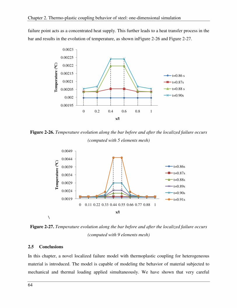
Chapter 2. Thermo-plastic coupling behavior of steel: one-dimensional simulation
64
failure point acts as a concentrated heat supply. This further leads to a heat transfer process in the
bar and results in the evolution of temperature, as shown inFigure 2-26 and Figure 2-27.
Figure 2-26. Temperature evolution along the bar before and after the localized failure occurs
(computed with 5 elements mesh)
\
Figure 2-27. Temperature evolution along the bar before and after the localized failure occurs
(computed with 9 elements mesh)
2.5 Conclusions
In this chapter, a novel localized failure model with thermoplastic coupling for heterogeneous
material is introduced. The model is capable of modeling the behavior of material subjected to
mechanical and thermal loading applied simultaneously. We have shown that very careful
0.00195
0.002
0.00205
0.0021
0.00215
0.0022
0.00225
0.0023
0 0.2 0.4 0.6 0.8 1
Tem
per
atu
re (
0C
)
x/l
t=0.86 s
t=0.87s
t=0.88 s
t=0.90s
0.0019
0.0024
0.0029
0.0034
0.0039
0.0044
0.0049
0 0.11 0.22 0.33 0.44 0.55 0.66 0.77 0.88 1
Tem
per
atu
re (
0C
)
x/l
t=0.86s
t=0.87s
t=0.88s
t=0.89s
t=0.90s
t=0.91s

Localized Failure for Coupled Thermo-Mechanics Problems
65
considerations of both theoretical formulation and finite element implementation are needed in
order to make such a development successful. The first main novelty of the proposed model with
respect to number of previous works is its capability to represent the mechanical behavior of the
material brought to localized failure and to account appropriately for the temperature induced
changes in material properties as well as for the heat conduction due to mechanical dissipation at
the localized failure surface.
The second important novelty concerns the optimal choice of finite element approximation
capable of accommodating the localized failure modes for coupled thermoplastic model. The
latter requires a careful combination of the displacement discontinuity to handle the localized
failure mode, the strain discontinuity to handle the material heterogeneities induced by the
heterogeneous temperature field along with the temperature dependence of material properties,
and the temperature gradient jump at the localized failure surface to account for the
corresponding discontinuity of heat flux. The finite element interpolations of this kind have been
elaborated for 1D case of 2-node truss-bar element.
The solution procedure for this class of problems exploits the adiabatic operator split. This
implies that the problem is first solved formechanics part (with adiabatic condition), and then for
heat transfer part. The former delivers the values of nodal displacementsand internal variables,
whereas the latter delivers the update of temperature field and the corresponding value of the
jump in the heat flux at the localized failure surface.It was shown that such a split provides the
most convenient implementation, and computational efficiency due to symmetry of tangent
operators.
The numerical examples shave shown that the temperature dependence of material properties
greatly influence the behavior of the bar. The most detailed study of this kind is performed in the
first example, showing that the bar properties linearly dependent on temperature can significantly
reduce the resistance of the truss-bar due to temperature increase. The same applies for non-
linear variation of properties with respect to temperature, as advocated in Eurocode1993. The
first example also shows that the temperature dependent properties can lead to large difference in
strain(even for the same stress value) in two sub-domains of a single truss-bar element separated
by the localized failure point.

Chapter 3. Behavior of concrete under fully thermo-mechanical coupling conditions
66
3 Behavior of concrete under fully thermo-mechanical coupling conditions
3.1 Introduction
In the previous chapter, we have studied on the thermo-elastoplastic with softening behavior of
steel, which was presented in one-dimensionalcase to clarify the theoretical model, as well as the
numerical solution for the problem. That model can be applied to model the behavior of the
rebarin reinforced concrete structure. To modeling the behavior of general reinforced concrete
structure, one have also to study on the thermo-mechanical behavior of the concrete material.
Previous works on the topic were carried out, for example see Galerkin et al.[45], Baker and de
Borst [36]. However, these works only consider the continuum damagebehavior and do not
consider the “ultimate” response. Futhermore, they do not provide a clear numerical solution for
the problem.
In this chapter, their two remaining deficiencies of problem will be removed. We first introduce
a new thermo-damage model, which is capable of modeling not only the continuum damagebut
also the softening behavior of concrete under thermo-mechanical coupling effect. By that way, a
united model can be applied to the hole concrete structure without “pre-chosing” a localized
failure region for the modeling structure ([40], [38]). The second novelty presented in this
chapter is a numerical solution for the problem, which is based on the “adiabatic” splitting
procedure and the embedded-discontinuity finite element method.
The outline of this chapter is as follows. In the next two sections, we introduce the theoretical
developments of the problem, which concentrate on the propagation of thermal effects through
the localized failure (the marco cracks). The discrete approximation of the problem and its
numerical solution using finite element method for the problem are presented in section 3.4.
Several illustrative examples are presented in section 3.5, followed by a conclusion in section
3.6.

Localized Failure for Coupled Thermo-Mechanics Problems
67
3.2 General framework
3.2.1 General continuum thermodynamic model
Several authors contributed to the thermo-damage coupling model, we can cite among others
Baker and de Borst [36], or Ngo et al. [44].
The starting point is the local form of the first principle of thermodynamics for the case of
thermo-mechanical inelastic response [17]:
),( eer εεσq (3-1)
Where r is the internal heat supply, q is the heat flux, σ is the stress field, ε is the strain field, e
is the internal stored energy and e is the reversible part of entropy ( denotes the time rate of
the variable ).
By following ([33], [42], [36]), the entropy is considered as the composition of the reversible
part (or “elastic” entropy) and irreversible part (or “inelastic” entropy):
de (3-2)
By the Legrendre transformation, the internal stored energy can be expressed in terms of the free
energy :
ee (3-3)
where denotes the absolute temperature of the media.
In thermo-damage framework, we can assume as the most generally accepted ([36], [44]) that
),,,( Dε is the function of the state variables: the total strain ε , the temperature , the
compliance tensor D and the hardening variable .
The Clausius-Duhem inequality for the model is written as:
eeeD εσεσint0 (3-4)
D
Dε
εσ deee
Dint0 (3-5)
In the case of “elastic” process, where 0D and 0 , the Clausius-Duhem inequality becomes
equal and therefore, the constitutive equations for the stress and the “elastic” entropy can be established:

Chapter 3. Behavior of concrete under fully thermo-mechanical coupling conditions
68
εσ
(3-6)
e
(3-7)
and the dissipation equation can also be written:
dD
D
Dint (3-8)
Also, by applying equation (3-3) and the constitutive equations (3-6), (3-7), the first principle of
thermodynamics can be rewritten:
eer εσq
eer
DD
εσε
q )(
er
D
Dq (3-9)
We also define of the second order tensor β which represents the relation between stress and
temperature, the heat capacity coefficient c and the tangent modulus C (see [44]):
εεσβ
2
:e
(3-10)
2
2
:
ee
ec (3-11)
12
:
Dεεε
σC
(3-12)
Note that the tangent stiffness tensor C is the inverse of the compliance damage tensor D. From
equation (3-10) and equation (3-12), we have
αDε
εσβ 1
(3-13)
Where εα : is the thermal expansion.
Note that in thermo-mechanical problem, the strain field is the composition of the mechanical
strain ( mε ) and the thermal strain ( ε ):
εεε m (3-14)
where the thermal strain is computed from the temperature and the thermal expansion:

Localized Failure for Coupled Thermo-Mechanics Problems
69
0 αε (3-15)
The free energy potential is chosen as the composition of mechanical energy ( m ) and the
thermal energy ( t ):
tm
cmm
0
0 ln2
1 εDε 1
(3-16)
tm
c
0
000 ln)]([)]([2
1 αεDαε 1 (3-17)
Where ϑ0 is the reference temperature and )( is the hardening energy.
With this definition of the free potential, the constitutive equation for stress and entropy can be
re-written:
0 αεD
εσ 1 (3-18)
00 ln)()(
c
e αεαD 1 (3-19)
The stress-like variable q associated to the hardening variable and Y to the compliance
damage tensor D are defined as:
:q (3-20)
σσαεDαεDD
Y 11
2
1)()(
2
1: 00
(3-21)
The internal dissipation of the media leads to the final result:
dqD DYint (3-22)
ther
mech
D
d
D
qD
σDσ2
1int (3-23)
where mechD and therD denote the mechanical and the thermal part of dissipation, respectively.
The damage threshold defining the elastic domain is chosen (see [25]) as:
qE
q f
e 1,,0 σDσσ (3-24)
Where De denotes the “thermo-mechanical” undamaged elastic compliance, f denotes the
Chapter 3. Behavior of concrete under fully thermo-mechanical coupling conditions
70
damage limit stress and d
dq
denotes the stress-like variable associated to (as introduced
above)
Considering the second principle of thermodynamics and the principle of maximum inelastic
dissipation we obtain the following evolution equations for internal variables:
Eq
D
q
int (3-25)
σDσD
DσDσ
σDσDσσ
e
e
e
eD int (3-26)
dD
int (3-27)
Where, is the Lagrange multiplier.
Considering equations (3-1) and (3-9) the system of local balance equation finally consists of the
force balance equation and the energy conservation equation (see [42], [36]).
rDint
0
q
bσ (3-28)
From the state equation (β0), we can compute the “elastic” entropy evolutionμ
00 ln)]([)(
c
e αεαD 1
ce
0))(()( αεαDDDαεαD 111
(3-29)
This equation, combined with equation (2), gives the following balance equations:
rDc
F
mech
c
),,(
0~~
))(()()(
0
Dε
1111 αεαDDDεαDqααD
bσ
(3-30)
where
0))(()(:),,( αεαDDDεαDDε 111 F (3-31)
is the structural heating (see[42], [36]), and
ααD 1 )(:~~ cc (3-32)
is the „modified‟ heat conduction of the material.

Localized Failure for Coupled Thermo-Mechanics Problems
71
3.2.2 Localized failure in damage model
3.2.2.1 Discontinuity of displacement field
Figure 3-1. Localized failure happens at crack surface and the “local” zone
In quasi-brittle materials, micro-cracks appear in the fracture process zone and will further
coalesce to generate macro crack. We assume in the following that such a failure happens in a
“local” zone x (see Figure 3-1). The failure can be represented by a strong discontinuity in the
displacement field across the surface x passing through point x (see [29], [52], [25], [24]),
which finally allows us to write the displacement field in the “local” zone x as follows:
)]()()[(),(ˆ),( xxuxuxu xttt (3-33)
where )(tu is the “jump” of displacement across the crack surface x (considered as constant in
x ), )(xx denotes the Heaviside function and )(x is a smooth function being 0 on x and 1
on x (where x and x are the boundary of two domains of the element separated by the
crack).
xfor
xforx
x 0
1)( (3-34)
The infinitesimal strain which corresponds to this displacement is given by:
sss
xtttt )()()()(),(ˆ),( xuxuxuxε (3-35)
where s is the symmetric part of .
We also note that xx
nx ss)( , where x is the Dirac function on x and n is the
x
y
Ω+
Ω-
x
x
x

Chapter 3. Behavior of concrete under fully thermo-mechanical coupling conditions
72
unit normal vector, then:
x
nuxuxuxuxε ssssttttt
x))(()()()()(),(ˆ),( (3-36)
The infinitesimal strain at the “local” zone can then be divided into a regular part and a singular part as:
xεxεxε )(),(),( ttt (3-37)
where: ssttt )()(),(ˆ),( xuxuxε (3-38)
and
stt ))(()( nuε (3-39)
3.2.2.2 Localized Free Energy
From the state equation (3-16) we can obtain the strain field in terms of the stress field as:
σDαxεαDxεDσ 00
11 ,, tt
σDαεxεx
)()(),( 0tt
(3-40)
By taking into account that the stress field must be bounded and assuming that there is no
thermal dilatation on the discontinuityx , the damage compliance tensor should be decomposed
into a singular part and a regular part (see [24], [25]):
xDDD (3-41)
so that:
σDαε )(),( 0tx on xx \
and
σDnuε stt )()(
on
x
The appearance of a “singular” part of the damage compliance tensor D leads to the
introduction of “singular” part of hardening variable , which controls the damage condition of
the material at the localization zone. Therefore, the hardening variable should also be split into
two parts:
x (3-42)
The decomposition of these state and internal variables allows us to write the decomposition of
the free energy into a regular part associated to the bulk and a singular part associated to
Localized Failure for Coupled Thermo-Mechanics Problems
73
the discontinuity x :
tm
c
0
000 ln2
1 αεDαε 1
x
nuDnu
αεDαε
sstt
c
1
000
10
2
1
ln2
1
(3-43)
By denoting 11
nDnQ the internal variable for describing the damage response at the
discontinuity (see [25]), we have the form of the singular part of free energy: ttm uQuQu 1
2
1,, (3-44)
We note here that the „thermal‟ energy does not appear in the singular part of the free energy (see
equation (3-44)), it is due to the assumption that there is no material (and therefore no heat
conductor) in the crack.
3.2.2.3 The dissipation and the evolution laws of internal variables
The dissipation of the material is computed by the equation
eedeeD εσεσint
deD εσint (3-45)
Note that the decomposition of the free energy and the strain lead to the decomposition of
entropy, so that equation (43) can be rewritten:
int
int
))((int
D
d
xx
e
D
detD
x unσεσ
t
(3-46)
The singular part of dissipation is:

Chapter 3. Behavior of concrete under fully thermo-mechanical coupling conditions
74
de
de
xx
x
xx
tD
tD
00
int
int
uu
t
ut
d
xD
Q
Qint (3-47)
where x denotes the temperature at the localized failure zone.
The formulation of singular part of internal dissipation allows us to find out the constitutive
equation for the singular part of state variables:
uQu
t 1
(3-48)
x
e
(3-49)
Singular parts of internal variables can also be computed:
Kq where
2
2
K (3-50)
ttYuQQuQ
Y
2
1)(
2
1 11
(3-51)
These state equations allow us to write the singular part of the internal dissipation in a similar
manner:
ther
mech
D
d
D
qD
tQt2
1int (3-52)
Where mechD and therD denote the mechanical part and the thermal part of the singular part of
internal dissipation.
Next step is to choose a failure criterion for the discontinuity, for that purpose, we base our work
on the multi-surface criterion proposed in (see [25]):
0),(
0),(
2
1
f
ss
f
mtt
ntt
(3-53)
where f is the given fracture stress, s is the limit value of shear stress on the discontinuity and
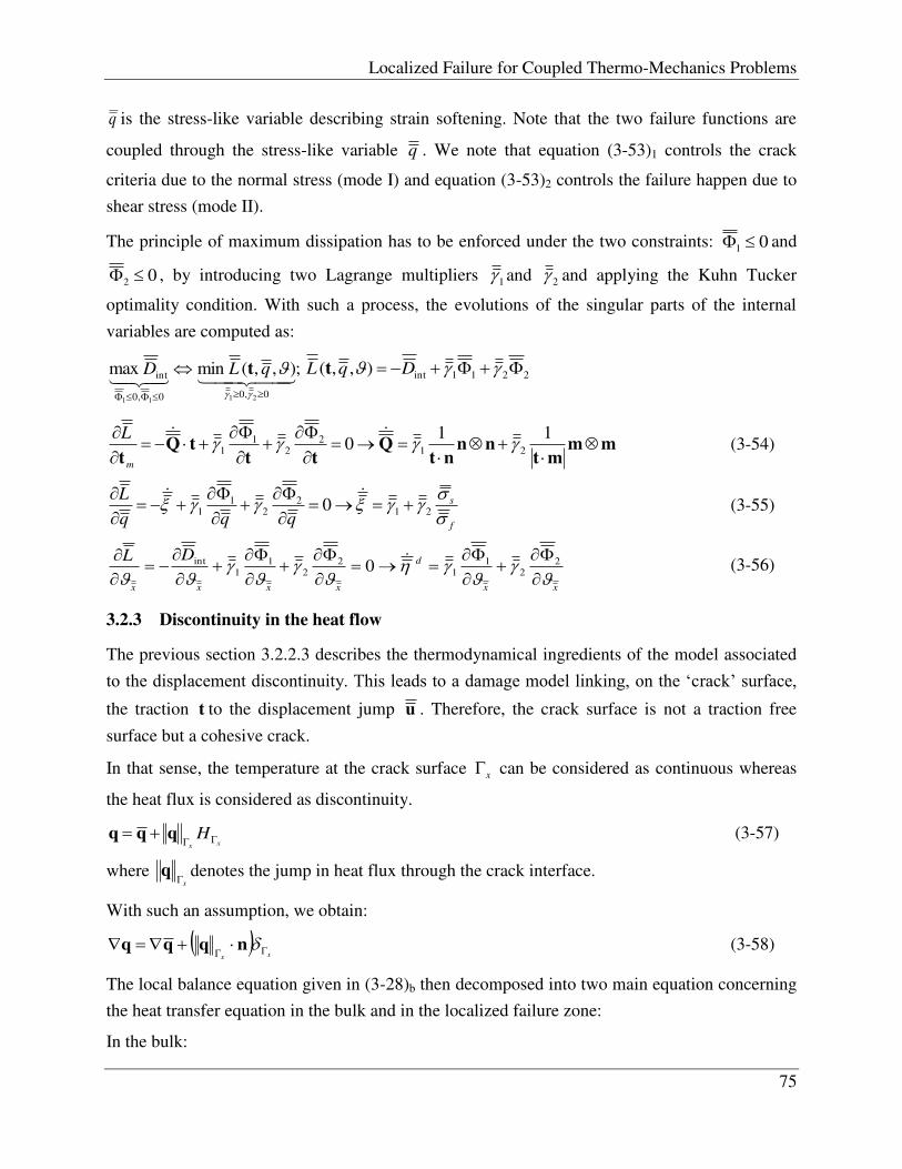
Localized Failure for Coupled Thermo-Mechanics Problems
75
q is the stress-like variable describing strain softening. Note that the two failure functions are
coupled through the stress-like variable q . We note that equation (3-53)1 controls the crack
criteria due to the normal stress (mode I) and equation (3-53)2 controls the failure happen due to
shear stress (mode II).
The principle of maximum dissipation has to be enforced under the two constraints: 01 and
02 , by introducing two Lagrange multipliers 1 and 2 and applying the Kuhn Tucker
optimality condition. With such a process, the evolutions of the singular parts of the internal
variables are computed as:
;),,(minmax0,00,0
int
2111
qLD t 2211int),,( DqL t
mmmt
nnnt
Qtt
tQt
11
0 212
21
1
m
L (3-54)
f
s
qqq
L
21
22
11 0
(3-55)
xx
d
xxxx
DL
22
11
22
11
int 0 (3-56)
3.2.3 Discontinuity in the heat flow
The previous section 3.2.2.3 describes the thermodynamical ingredients of the model associated
to the displacement discontinuity. This leads to a damage model linking, on the „crack‟ surface, the traction t to the displacement jump u . Therefore, the crack surface is not a traction free
surface but a cohesive crack.
In that sense, the temperature at the crack surface x can be considered as continuous whereas
the heat flux is considered as discontinuity.
xx
H qqq (3-57)
where xq denotes the jump in heat flux through the crack interface.
With such an assumption, we obtain: xx
nqqq (3-58)
The local balance equation given in (3-28)b then decomposed into two main equation concerning
the heat transfer equation in the bulk and in the localized failure zone:
In the bulk:
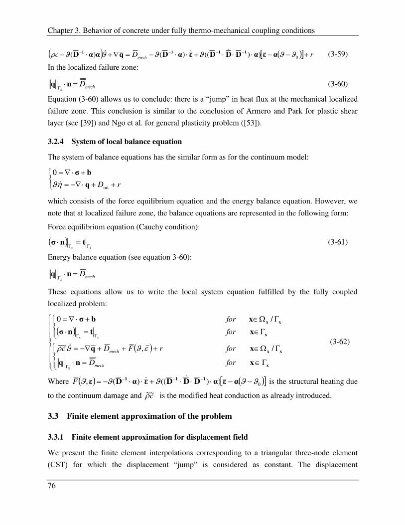
Chapter 3. Behavior of concrete under fully thermo-mechanical coupling conditions
76
rDc mech 0))(()()( αεαDDDεαDqααD 1111
(3-59)
In the localized failure zone:
mechDx
nq (3-60)
Equation (3-60) allows us to concludeμ there is a “jump” in heat flux at the mechanical localized failure zone. This conclusion is similar to the conclusion of Armero and Park for plastic shear
layer (see [39]) and Ngo et al. for general plasticity problem ([53]).
3.2.4 System of local balance equation
The system of balance equations has the similar form as for the continuum model:
rDint
0
q
bσ
which consists of the force equilibrium equation and the energy balance equation. However, we
note that at localized failure zone, the balance equations are represented in the following form:
Force equilibrium equation (Cauchy condition):
xx tnσ (3-61)
Energy balance equation (see equation 3-60):
mechDx
nq
These equations allow us to write the local system equation fulfilled by the fully coupled
localized problem:
x
xx
x
xx
xnq
xq
xtnσxbσ
x
forD
forrFDc
for
for
mech
mech
xx
/,~~
/0
(3-62)
Where 0))(()(, αεαDDDεαDε 111 F is the structural heating due
to the continuum damage and c~~ is the modified heat conduction as already introduced.
3.3 Finite element approximation of the problem
3.3.1 Finite element approximation for displacement field
We present the finite element interpolations corresponding to a triangular three-node element
(CST) for which the displacement “jump” is considered as constant. The displacement

Localized Failure for Coupled Thermo-Mechanics Problems
77
discontinuity is taken into account by introducing an additional shape function )(xM1 , then the
following approximation is considered for the displacement field:
tM1
N
a
aa
nodes
uxdxNxd )()()(1
(3-63)
where Na(x) is the vector of isoparametric shape function for CST element, ad is the vector of
displacement at node a, u is the vector of displacement “jump” and M1(x) is the additional shape
function with unit “jump” on x , represented in Figure 3-2.
The strain field interpolation therefore becomes:
uxGdxBxε 1r nodesN
a
aat1
),( (3-64)
where xLNxB aa and xLxG1r 1M , L denotes the matrix form of the strain-
displacement operator s . Due to the form of M1(x), G1r(x) is decomposed into a regular part
and a singular part as:
x xGxGxG rrr 111 (3-65)
( x denotes the discontinuity surface, n
and m
the unit normal and tangential vectors to x )
3.3.2 Finite element interpolation function for temperature
Equation (3-60) shows that there is a “jump” in heat flux through the cracking surface due to the localized mechanical dissipation and also indicates a different evolution of temperature on each
x
m
n
1
2
3
Figure 3-2. Additional shape function M1(x) for displacement
discontinuity

Chapter 3. Behavior of concrete under fully thermo-mechanical coupling conditions
78
side of the discontinuity surface due to thermo-mechanical dissipation. This evolution should be
taken into account in the interpolation function for temperature (see Figure 3-3).
xdxNxxx 21
2 MMdNnodesN
a
aa (3-66)
Where ad denotes the temperature at node a, x
aN is the iso-parametric shape function, is the
evolution of temperature at the localized failure point related to the heat flux “jump” on x ,
x2M is an additional shape function (see Figure 3-3) ; the latter allows to take into account the
different evolution of temperature on each side of the discontinuity due to the modification in
heat conduction produced by the discontinuity x and the localized mechanical dissipation
taking place on x .
If we assume that the crack line is passing through the gravity point (x6,y6) of the triangular
three-node element then x2M has the following form:
x
x
x
,))((
3
)(])())[((
)(
26232326
232223
16141416
144161416141
2
yyxxyyxx
xxyyxxyy
yyxxyyxx
yyzyyxxzxxxxyy
M
(3-67)
55 , yx
66 , yx
44 , yx 22 , yx
-1
n
11, yx
33 , yx
x
y
0
Figure 3-3. Additional shape function

Localized Failure for Coupled Thermo-Mechanics Problems
79
x
x(x
x
x(x
xxG
ifyyxxyyxx
xx
ifyyxxyyxx
xxzxx
y
M
ifyyxxyyxx
yy
ifyyxxyyxx
yyzyy
x
M
M
26232326
23
16141416
14416
26232326
23
16141416
14416
2
3)
3)
)()(
2
2
2
(3-68)
where (x1,y1); (x2,y2) and (x3,y3) are the coordinates of the three nodes, (x4,y4), (x5,y5) are the
coordinate of the point at the intersection of the crack line and the element edges and z4 is
defined as:
26232326
242323244
))((
yyxxyyxx
xxyyxxyyz
(3-69)
3.3.3 Finite element equation for the problem
We start from the strong form of equilibrium equation for the thermomechanical problem
(equation (3-62))
x
xx
x
xx
xnq
xq
xtnσxbσ
x
forD
forrFDc
for
for
mech
mech
xx
/,~~
/0
(3-70)
We note that this equation is time dependent (in particular, the thermal transfer process is non-
stationary), so the problem should be solved by time linearization method. In particular, the
whole process is divided into many time steps (Δ ), and the problem turns into identifying the
mechanical and thermal variables at the next time step (n+1) by assuming that the mechanical
and thermal variables at the current time step (n) are already known. This linearization method
will be discussed in detail in the following.
3.3.3.1 For mechanical balance equation
For mechanical balance equation (70)1, by applying incompatible mode method (see [17], [18],
[25]), we can establish the following form of the discretized equation:

Chapter 3. Behavior of concrete under fully thermo-mechanical coupling conditions
80
x
xx
xutGεσGh
xffA
forddt
fortt
e x
x
x
elem
T
v
eT
v
e
e
ext
e
int
N
e
0,,
/01
(3-71)
where x
evver
e
rv dA
x xGxGxGGxG 11111
1 is the “modified” interpolation
function of “virtual” strain, which is chosen different from the interpolation function of “real”
strain xG r1 in order to satisfy the “patch test” (see [18]) and e
Tedtf
xe
,/int εB .
By taking into account the interpolation function of strain and temperature: tt r uGBdε 1 ,
2Mta dN ,
1
2 xdxN Maax , equation (72) can be brought to the linearized
form:
Given nnnn u ,,, dd find i
n
i
n
i
n
i
n
1111 ,,, dud
i
nx
i
n
T
v
i
n
e
i
n
T
v
i
nx
i
n
T
v
i
nx
i
n
T
v
i
n
e
i
n
T
v
i
n
e
i
n
T
v
i
n
e
i
n
T
v
i
n
e
i
n
T
v
ie
n
i
n
iext
n
i
ne
i
n
i
ne
i
n
i
ne
i
n
i
ne
i
n
xxxx
eeee
ee
ee
dddd
dddd
ttdd
dd
,1
1
,1
1
11
11
,1
1
,1
1
11
11
)(1
)int(1
)(1
,1
1
,1
1
)(1
1
)(1
1
)()(
tGd
d
σGu
u
tGd
d
tG
σGd
d
σGu
u
σGd
d
σGh
ffσ
Bdd
σB
uu
σBd
d
σB
tt
tt
(3-72)
3.3.3.2 For thermal balance equation
The thermal balance equation is taken from equation (3-70)2 :
x
xx
xnq
xDεq
x
forD
forrFDc
mech
mech /,,~~
`
(3-73)
By applying the Fourier laws kq for this problem, we have:
at continuum domain: xx /x :
2 kk qq (3-74)
at the crack surface x :

Localized Failure for Coupled Thermo-Mechanics Problems
81
xx
x
xx
xxx
kMdNkk aaa
)( 222
nq
(3-75)
where k is the heat conductivity coefficient of the material at continuum domain and x
k is the
heat conductivity coefficient at the localized failure zone.
By combining equation (75) and equation (73)b, we obtain the equation to determine μ
xk
Dmech
(3-76)
If we introduce xw the virtual temperature field and using the Fourier equation for heat flux
kq then the weak form of equation (74)a becomes:
0,~~///1
x
e
add
eqxe
xe
el
drFDwdqwdkwdcwA
R
mecheqn
N
e ε
(3-77)
If the iso-parametric interpolation function is used for the virtual temperature
wNx aa wNw then we can establish discrete version of this equation as follows:
xe
eq
el
xe
xe
el
dRdqA
dkdMcA
add
T
eqn
TN
e
T
2
TN
e
/
,,
1
/
,
/
,
1
~~
wNwN
GdBwBdNwN 2
(3-78)
Note that this equation should be valid for any value of virtual temperature, thus we have:
1
11 QFdKPdM
elel N
e
eeeeN
eAA
(3-79)
where
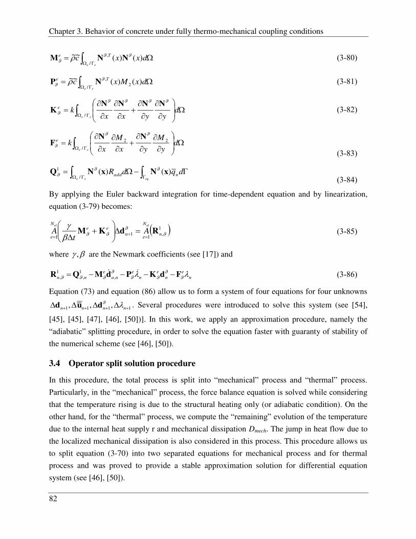
Chapter 3. Behavior of concrete under fully thermo-mechanical coupling conditions
82
xe
dxxcTe
/
, )()(~~ NNM
(3-80)
xe
dxMxcTe
/ 2, )()(~~ NP
(3-81)
xe
dyyxx
ke
/
NNNNK
(3-82)
xe
dy
M
yx
M
xk
e
/
22
NNF
(3-83)
eqxe
dqdR nadd )()(/
1 xNxNQ (3-84)
By applying the Euler backward integration for time-dependent equation and by linearization,
equation (3-79) becomes:
1,
11
1
n
N
en
eeN
e
elel
At
A RdKM
(3-85)
where , are the Newmark coefficients (see [17]) and
n
e
n
e
n
e
na
e
nn FdKPdMQR ,
1,
1,
(3-86)
Equation (73) and equation (86) allow us to form a system of four equations for four unknowns
1111 ,,, nnnn dud . Several procedures were introduced to solve this system (see [54],
[45], [45], [47], [46], [50])]. In this work, we apply an approximation procedure, namely the
“adiabatic” splitting procedure, in order to solve the equation faster with guaranty of stability of
the numerical scheme (see [46], [50]).
3.4 Operator split solution procedure
In this procedure, the total process is split into “mechanical” process and “thermal” process. θarticularly, in the “mechanical” process, the force balance equation is solved while considering that the temperature rising is due to the structural heating only (or adiabatic condition). On the
other hand, for the “thermal” process, we compute the “remaining” evolution of the temperature due to the internal heat supply r and mechanical dissipation Dmech. The jump in heat flow due to
the localized mechanical dissipation is also considered in this process. This procedure allows us
to split equation (3-70) into two separated equations for mechanical process and for thermal
process and was proved to provide a stable approximation solution for differential equation
system (see [46], [50]).

Localized Failure for Coupled Thermo-Mechanics Problems
83
“εechanical” processμ
),,())(()(~~0
/0
0 DεαεαDDDεαD
xtnσxbσ
111
x
xx
Fc
for
for
e
xx
(3-87)
“Thermal” processμ
xmech
mech
forD
forrDc
xnq
xq
x
xx /~~
(3-88)
The overall scheme of adiabatic splitting operation is described in Figure 3-4.
We present in the following the different steps of the adiabatic scheme in detail beginning by the
“mechanical process”.
3.4.1 Mechanical process
3.4.1.1 Mechanical process in continuum damage
In this part, we go back to the theoretical formulation to highlight the modification induced by
the adiabatic condition considered in our numerical scheme. The evolution of the temperature
due to structural heating (equation (3-87)b) is established for adiabatic condition by the equation:
xx
tnσbσ0
mech
mech
D
RDc
x
nq
q ~~
11, nn ud
0e mechmech DD ,
0e
nn u,d Displacement
Temperature
t(s)
Tn+1 Tn
Figure 3-4. “Adiabatic” splitting procedure.
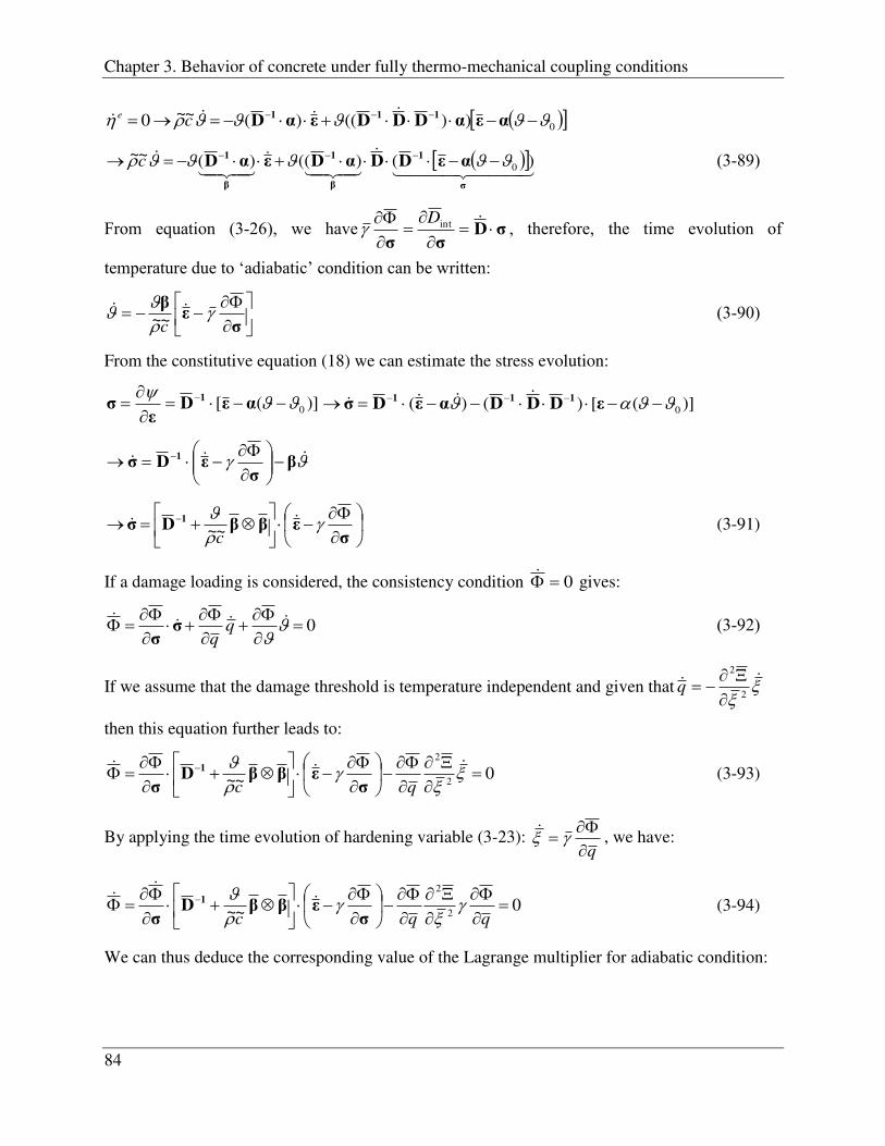
Chapter 3. Behavior of concrete under fully thermo-mechanical coupling conditions
84
0))(()(~~0 αεαDDDεαD 111 ce
σ
1
β
1
β
1 αεDDαDεαD )()(()(~~0
c (3-89)
From equation (3-26), we have σDσσ
intD , therefore, the time evolution of
temperature due to ‘adiabatic’ condition can be written:
σ
εβ
c~~ (3-90)
From the constitutive equation (18) we can estimate the stress evolution:
)]([ 0 αεD
εσ 1 )]([)()( 0 εDDDαεDσ 111
βσ
εDσ 1
σεββDσ 1
c~~ (3-91)
If a damage loading is considered, the consistency condition 0 gives:
0
q
qσ
σ
(3-92)
If we assume that the damage threshold is temperature independent and given that 2
2
q
then this equation further leads to:
0~~ 2
2
qc σεββD
σ1 (3-93)
By applying the time evolution of hardening variable (3-23): q , we have:
0~~ 2
2
qqc
σεββD
σ1
(3-94)
We can thus deduce the corresponding value of the Lagrange multiplier for adiabatic condition:

Localized Failure for Coupled Thermo-Mechanics Problems
85
ε
σββD
σ
ββDσ
1
1
2
2
2
~~
~~
qc
c
(3-95)
The rate form of the constitutive equation which can be used to compute the evolution of each
internal variable is finally given for mechanical part as:
0
~~
~~
~~
0)~~(
2
2
2
if
qc
c
c
ifc
ε
σββD
σ
σββD
σββDσ
εββDσ
1
1
1
1
(3-96)
Or in short:
εCσ ad (3-97)
Before carrying out the global computation, we have to estimate some ingredients including:
mechanical internal variables, „adiabatic‟ tangent modulus (Cad) and updated stress. These
computations should be performed at the element level, or in other word, at the local level. An
algorithm to calculate these variables by using „return-mapping‟ algorithm (see [51])is
introduced in Figure 3-5.
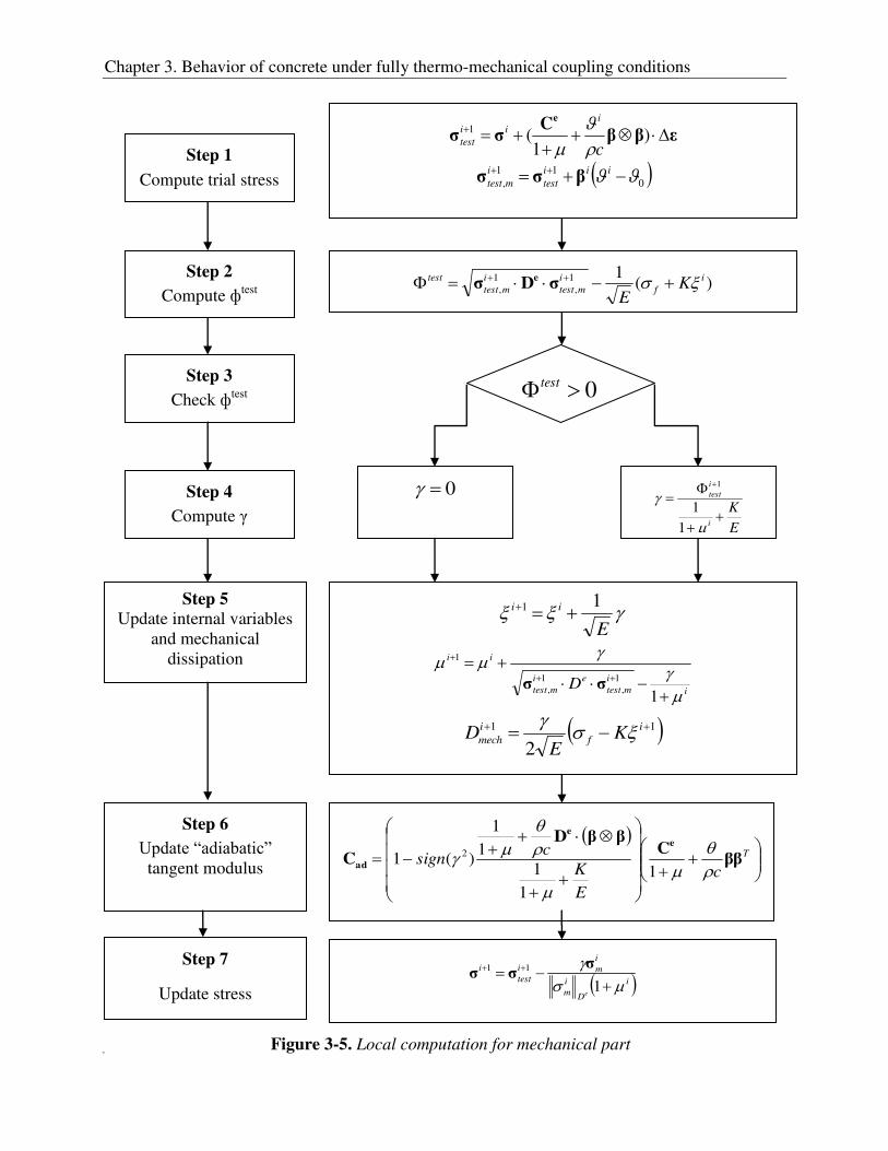
Chapter 3. Behavior of concrete under fully thermo-mechanical coupling conditions
86
Step 1
Compute trial stress
εββCσσe )
1(1
c
iii
test
011
, iii
test
i
mtest βσσ
Step 2
Compute фtest )(11
,1
,i
f
i
mtest
i
mtest
testK
E σDσ e
Step 3
Check фtest
Step 4
Compute
0
E
Ki
i
test
1
1
1
Step 5 Update internal variables
and mechanical dissipation
E
ii 11
i
i
mtest
ei
mtest
ii
D
11
,1
,
1
σσ
11
2 i
f
i
mech KE
D
T
c
E
K
csign ββC
ββD
Ce
e
ad
1
1
11
1
)(1 2
Step 6
Update “adiabatic” tangent modulus
i
D
i
m
i
mi
test
i
e
111 σσσ
Step 7
Update stress
0test
Figure 3-5. Local computation for mechanical part
Localized Failure for Coupled Thermo-Mechanics Problems
87
3.4.1.2 Mechanical process at localized failure
The localized failure in this case happens due to mechanical loading only. The irregular part of
the Lagrange multiplier is determined from the consistency condition: 01 and/or 02 which
leads to:
Strong failure due to normal stress: 00 111
q
q
t
t (3-98)
Strong failure due to shear stress: 00 222
q
q
t
t (3-99)
Where KqKq (for linear isotropic softening)
The evolution of traction can be established from the state equation (3-45):
uQt 1
2
1
1
k
kk
tQuQtuQQQuQt 1
t
111
(3-100)
These equations finally lead to the following expressions for Lagrange multipliers:
2,1;
k
qK
q
kkkk
k
k u
tQ
t
Qt
1
1
(3-101)
And the rate constitutive equation between traction and “jump” in displacement can be established:
0
0
k
kkkk
n
kk
k
if
qK
q
if
u
tQ
t
tQQ
tQt
uQt
1
11
1
1
(3-102)
uCt ad (3-103)
3.4.1.3 Finite element method for “mechanical” process
By applying the “adiabatic” spitting procedure, we can establish the evolution of stress and
traction due to the evolution of strain and displacement “jump” with “adiabatic” tangent modulus

Chapter 3. Behavior of concrete under fully thermo-mechanical coupling conditions
88
(equation (3-97) and (3-104)). This allows us to write the linearization form of equation (3-72)
without the temperature evolution:
i
n
i
n
ie
nv
i
n
Tie
nv
ie
n
i
n
iext
n
i
n
ie
nr
i
n
ie
n tt
11,,
1,1,,1,
)(1
)int(1
)(1
)(1
,1,
)(1
,1 )()(
uKHdFh
ffuFdK
(3-104)
where
ee
e
iad
n
T
e
i
n
Tie
n dd BCBd
σBK ,
11
)(,1
(3-105)
ee
eiad
n
T
v
e
i
n
T
v
Tie
nv dd BCGd
σGF ,
11
),(,1,
(3-106)
ee
e
r
iad
n
T
v
e
i
n
T
v
ie
n dd GCGu
σGH ,
11
)(,1
(3-107)
ian
n
e
x
i
n
T
v
i
n xx
ld,
11
)(1,
Cu
tGK
(3-108)
where e
xl is the length of the crack for the consider element.
Equation (3-104) can be solved by an operator split, where 1 nu is solved at the element level
and 1 nd is solved at the global level (see [25]). By that way, from equation (3-104)2 we can
compute:
in
Tie
nv
i
n
ie
nv
i
n 1,,1,
1
1,,
1,1
dFKHu (3-109)
By using static condensation at the element level, the system (3-104) is reduced to:
)()(ˆ )int(1
)(1
1
)(1
,1
1ttAA
i
n
iext
n
N
e
i
n
ie
n
N
e
elel
ffdK
(3-110)
where
Tie
nv
i
n
ie
nv
ie
nr
ie
n
ie
n
,,1,
1
1,,
1,,
1,,
1,
1ˆ
FKHFKK
(3-111)
is the modified element tangent stiffness.
3.4.2 Thermal process
ηnce the “mechanical” process is solved, the mechanical dissipation and the evolution of the displacement “jump” are known. We can introduce these values to the equation (3-83) to solve
the “remaining” evolution of temperature and also the “jump” in the heat flow through the crack
Localized Failure for Coupled Thermo-Mechanics Problems
89
surface. Note that the evolution of temperature in this process is due to mechanical dissipation,
internal heat supply and external heat source (and does not include the structural heating, which
was computed before in the “mechanical” process). We obtain then the following form for equation (3-85)
1,1
~~
nn
ee
tRdKM
(3-112)
where
n
e
n
e
n
e
na
e
n FdKPdMQR ,
11,
~~
(3-113)
eqe
dqdR na
n
addax )(~
)(~ 1
13, xNxNQ (3-114)
xk
Dn
mechn
(3-115)
rDRn
mech
n
add ~ (3-116)
Where n
mechD and n
mechD denote the regular part and the singular part of the mechanical
dissipation at time step „n‟.

Chapter 3. Behavior of concrete under fully thermo-mechanical coupling conditions
90
3.5 Numerical Examples
In this section, several illustrative numerical examples are presented in order to show the
capability of the proposed model. In these examples, the material properties of concrete are
temperature dependent with the relations taken from Nielsen et al. (see [55]) and Eurocode 1992
(see [7]). In particular, the following equations are used:
For Young modulus:
2
20 10000
2010
CEE (3-117)
For hardening modulus:
2
20 10000
2010
CKK
(3-118)
For facture stress:
CCfor
CCfor
Cff
Cff
00
20,
00
20,
600100500
1001
10020
0
0
(3-119)
The same relation is used for tensile stress:
CCfor
CCfor
Cff
Cff
00
20,
00
20,
600100500
1001
10020
0
0
(3-120)
For specific heat
CCforkgK
Nmmc
CCforkgK
Nmmc
CCforkgK
Nmmc
CCforkgK
Nmmc
p
p
p
p
006
0066
0066
006
1200400101.1
400200102000
200101
200100101000
100109.0
10020109.0
(3-121)
For mass density

Localized Failure for Coupled Thermo-Mechanics Problems
91
CCfor
CCfor
CCfor
CCfor
C
C
C
C
00
20
00
20
00
20
00
20
1200400800
40007.095.0
400200200
20003.098.0
20011585
11502.01
11520
0
0
0
0
(3-122)
and for thermal conductivity (upper limit)
CCfork00
2
120020100
0107.0100
2451.02
(3-123)
All computations are performed by a research version of the finite element analysis program
FEAP (see [56], [57]).
3.5.1 Tension Test and Mesh independency
We consider here a concrete plate (300mm – 200mm) fixed in its left edge. Material properties at
the reference temperature (200C) are given in Table 3-1.
Table 3-1. Material Properties
Material Properties Values Units
Young modulus (C
E 020) 38000 MPa (N/mm2)
Fracture stress (Cf
020, ) 2.00 MPa (N/mm2)
Isotropic hardening modulus (C
K 020) 4000 MPa (N/mm2)
Tensile stress Cf
020, 3.00 MPa (N/mm2)
Mass density (C020
) 2.5×10⁻⁶ kg.mm-3
3.5.1.1 Mesh independency
We start by studying the mesh independency of the proposed strategy. To that end, the problem
is solved with two different meshes: a coarse mesh (15x5x2 elements) and a fine mesh (24x10x2
elements) in order to show the mesh independency of the method. The concrete plate is subjected
to an increasing imposed displacement at the right edge, which increases from 0 mm to 0.2 mm
in 100s and then decreases back to 0 mm also in 100 s. In order to drive the localization (the test
performed is homogeneous), a material defect at the middle of the bottom edge (by reducing

Chapter 3. Behavior of concrete under fully thermo-mechanical coupling conditions
92
from 3.0 MPa to 2.9 MPa the ultimate strength). Received results are showed in Figure 3-6,
Figure 3-7, Figure 3-8 and Figure 3-9.
Coarse mesh Fine Mesh
Figure 3-6. Temperature distribution in the plate at t = 20s
Coarse mesh Fine Mesh
Figure 3-7. Temperature distribution in the plate at t = 52.4s
Coarse mesh Fine Mesh
Figure 3-8. Temperature distribution in the plate at t = 100s

Localized Failure for Coupled Thermo-Mechanics Problems
93
Coarse mesh Fine mesh
Figure 3-9. Load/Displacement Curve for the coarse and the fine mesh
Figure 3-6, Figure 3-7 and Figure 3-8 describe the evolution of temperature during the loading
process at the plate, while the load/displacement curve of the plate is plotted in Figure 3-9 and
the relationship between the traction and the crack opening in the localization failure at the
0 0.02 0.04 0.06 0.08 0.1 0
0.5
1
1.5
2
2.5
3
Crack Opening Width (mm)
Traction (MPa)
Loading
Loading
Unloading
Fine Mesh
Coarse Mesh
0.04 0.08 0.12 0.16 0.2 0
100
200
300
400
500
600
Displacement (mm)
Force (N/mm)
0.04 0.08 0.12 0.16 0.2 0
100
200
300
400
500
600
Displacement (mm)
Force (N/mm)
Figure 3-10. Traction - Crack Opening relation at the localized failure

Chapter 3. Behavior of concrete under fully thermo-mechanical coupling conditions
94
middle of the bottom edge is shown in Figure 3-10.
We can find out in Figure 3-6 that: for the loading state corresponding to t = 20s, the plate works
in continuum damage threshold, the damage is uniformly distributed in all the material which
leads to the uniform distribution of temperature; after that at t = 52.4s, the localization failure
happens on the defect (at the middle of the bottom edge) and the localized mechanical
dissipation becomes a heat source which helps raising the temperature at this position; the
localization failure then propagates from the defect to the top edge of the plate and the
temperature continues to rise and transfer from the localization zone to the neighbor zone (Figure
3-7). At the final loading state (t = 100s) (see Figure 3-8), the final crack line exists through the
height of the plate with the direction perpendicular to the principal stress, the temperature raising
due localization is largest at the defect ( C035.0 ) and smaller at the middle of the plate (
C025.0 ). These values are relative small but much larger than the temperature raising due
to “continuum” mechanical dissipation, which is C04103.2 ( see Figure 3-6 and Figure
3-7)
Figure 3-9 and Figure 3-9 show the perfect „match‟ of the load/displacement curve and the
between traction/crack opening curve taken for the two meshes. It is clear from these figures
that the mechanical behavior of the concrete plate does not depend on the mesh. These results
prove the mesh-independency of the method.
3.5.1.2 Concrete plate subjected to coupling thermo-mechanical loadings
In this test, we consider the behavior of the concrete under two others thermo-mechanical
loading cases. For the first loading case, the plate is simultaneously subjected to an imposed
displacement at the right edge (increasing with the velocity 0.002 mm/s) and an imposed
temperature applied at the bottom edge (increasing with the velocity 50C/s). For the second
loading case, the plate is firstly heated at its bottom until 5000C and then submitted to an
imposed displacement at the right edge (with the velocity = 0.002 mm/s). Figure 3-11 shows the
load/displacement curves of these two thermo-mechanical loading cases in comparison to the
mechanical loading case introduced in section 3.5.1.

Localized Failure for Coupled Thermo-Mechanics Problems
95
Figure 3-11 clearly illustrates the effect of temperature loading on the mechanical behavior of the
concrete plate. The „mechanical‟ bearing resistance of the concrete plate significantly reduces for the two thermo-mechanical loading cases in comparison to the mechanical loading case. In
particular, the imposed displacement which leads to localized failure in the plate reduce from
0.115 mm in the mechanical loading case to 0.086 mm in the first thermo-mechanical loading
case and then to 0.038 mm in the second thermo-mechanical loading case. This is the
consequence of the reduction of material properties of concrete in high temperature as well as the
effect of thermal stress in the plate.
3.5.2 Simple bending test
We consider a short beam (h =200mm, l=200mm) fixed at its left edge. The material properties
are the same as for the first example (see Table 1). Two loading cases are considered for this
example: (1) the beam is submitted to mechanical loading only, in which the right edge is
submitted to vertical imposed displacement (increasing from 0mm to 0.16mm in 100s and then
reduces to 0mm in also 100s); (2) the beam is submitted to mechanical loading as in the first
loading case and also an imposed temperature at its fixed edge (which increasing from 00C to
0 0.02 0.04 0.06 0.08 0.1 0.12 0.14 0.16 0.18 0.2 0
100
200
300
400
500
600
Displacement (mm)
Force (N/mm)
Thermo-mechanical loading (case 2)
Thermo-mechanical loading (case 1)
Mechanical loading only
Figure 3-11. Load/ Displacement Curve of the plate in thermo-mechanical loadings

Chapter 3. Behavior of concrete under fully thermo-mechanical coupling conditions
96
5000C in 100s and then decreasing to 00C in another 100s).
Figure 3-12 shows the temperature evolution for the first loading case, in which we can figure
out the evolution of temperature due to continuum damage (at t =10s) and due to localization
failure (at t =89.5s and t = 100s). We note that the temperature is mainly distributed in the fixed
edge of the beam (where the stress is large). The value of temperature is very small when the
beam is working in the continuum damage behavior but significantly increases when localized
failure happens (from C06
max 1075.1 at t = 10s to C0
max 157.0 at t = 89.5s then to
C0
max 22.0 at t = 100s). It is also interesting to note that the temperature continue to rising in
the beam in the unloading state (see Figure 3-12). The remaining temperature will further lead to
the existing of the remaining stress in the beam after unloading (as showed in Figure 3-14).
The temperature evolution in the beam for the second loading case is presented in Figure 3-13.
The temperature remaining in the beam in this case is different to the temperature remaining in
the first loading case and is mainly due to the temperature propagation from the external heat
source.
In both two cases, the initial cracks are detected in the bottom-left zone of the beam, where the
maximum principle stress is greatest (see Figure 3-14 and Figure 3-15). The crack then
propagates into the middle fiber of the beam in the vertical direction. This phenomena is really
suitable to the expected behavior of the beam in bending.
The load-displacement curves for both loading cases are plotted in Figure 3-16. We can again
identify the contribution of temperature loading in the mechanical response of the beam in the
elastic state, the continuum damage state and also the localized failure state. In particular, this
figure clearly shows that the bending resistance of concrete beam significantly reduces when
submitted to thermal loading.
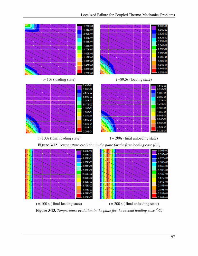
Localized Failure for Coupled Thermo-Mechanics Problems
97
t= 10s (loading state) t =89.5s (loading state)
t =100s (final loading state) t = 200s (final unloading state)
Figure 3-12. Temperature evolution in the plate for the first loading case (0C)
t = 100 s ( final loading state) t = 200 s ( final unloading state)
Figure 3-13. Temperature evolution in the plate for the second loading case (0C)

Chapter 3. Behavior of concrete under fully thermo-mechanical coupling conditions
98
t = 10s (final loading state)
t = 20s (final unloading state)
Figure 3-14. Evolution of maximum principal stress for the first loading case (MPa)
t = 10s (final loading state)
t = 20s (final unloading state)
Figure 3-15. Evolution of maximum principal stress for the second loading case (MPa)
Figure 3-16. Load/ Displacement curve for 2 loading cases
0 0.02 0.04 0.06 0.08 0.1 0.1 0.1 0.16
20
40
60
80
100
120
140
160
180
Displacement
Force (N/mm)
Loading case 1
Loading case 2
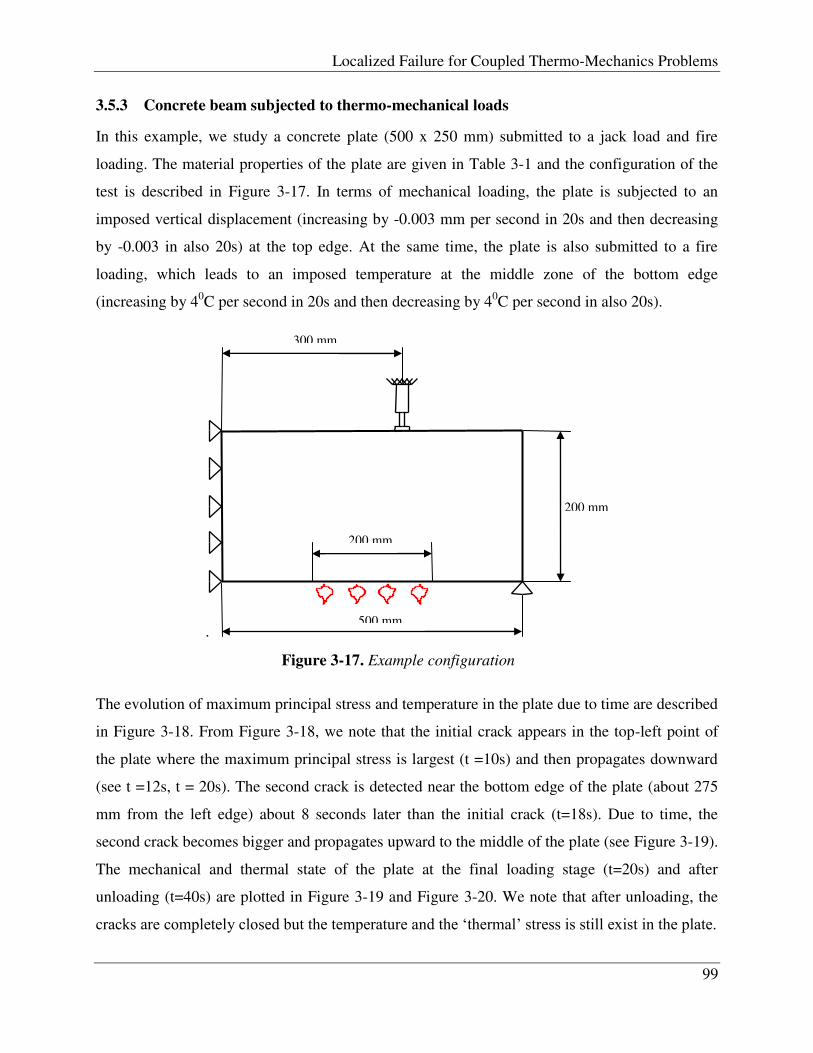
Localized Failure for Coupled Thermo-Mechanics Problems
99
3.5.3 Concrete beam subjected to thermo-mechanical loads
In this example, we study a concrete plate (500 x 250 mm) submitted to a jack load and fire
loading. The material properties of the plate are given in Table 3-1 and the configuration of the
test is described in Figure 3-17. In terms of mechanical loading, the plate is subjected to an
imposed vertical displacement (increasing by -0.003 mm per second in 20s and then decreasing
by -0.003 in also 20s) at the top edge. At the same time, the plate is also submitted to a fire
loading, which leads to an imposed temperature at the middle zone of the bottom edge
(increasing by 40C per second in 20s and then decreasing by 40C per second in also 20s).
.
The evolution of maximum principal stress and temperature in the plate due to time are described
in Figure 3-18. From Figure 3-18, we note that the initial crack appears in the top-left point of
the plate where the maximum principal stress is largest (t =10s) and then propagates downward
(see t =12s, t = 20s). The second crack is detected near the bottom edge of the plate (about 275
mm from the left edge) about 8 seconds later than the initial crack (t=18s). Due to time, the
second crack becomes bigger and propagates upward to the middle of the plate (see Figure 3-19).
The mechanical and thermal state of the plate at the final loading stage (t=20s) and after
unloading (t=40s) are plotted in Figure 3-19 and Figure 3-20. We note that after unloading, the
cracks are completely closed but the temperature and the „thermal‟ stress is still exist in the plate.
300 mm
200 mm
500 mm
200 mm
Figure 3-17. Example configuration

Chapter 3. Behavior of concrete under fully thermo-mechanical coupling conditions
100
Maximum principal stress at t = 8 s Temperature distribution at t = 8s
Maximum principal stress at t = 10 s Temperature distribution at t = 10s
Maximum principal stress at t = 12 s Temperature distribution at t = 12s
Maximum principal stress at t = 18 s Temperature distribution at t = 18s
Figure 3-18. Evolution of maximum principal stress and temperature due to time
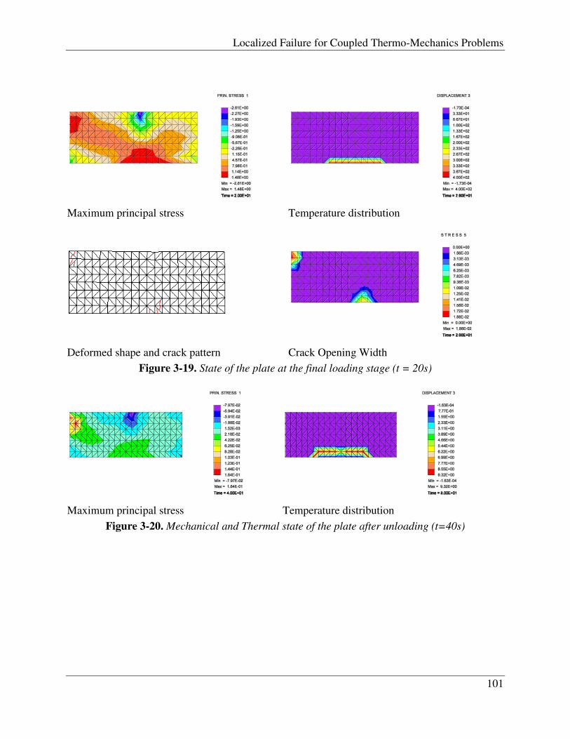
Localized Failure for Coupled Thermo-Mechanics Problems
101
Maximum principal stress Temperature distribution
Deformed shape and crack pattern Crack Opening Width
Figure 3-19. State of the plate at the final loading stage (t = 20s)
Maximum principal stress Temperature distribution
Figure 3-20. Mechanical and Thermal state of the plate after unloading (t=40s)
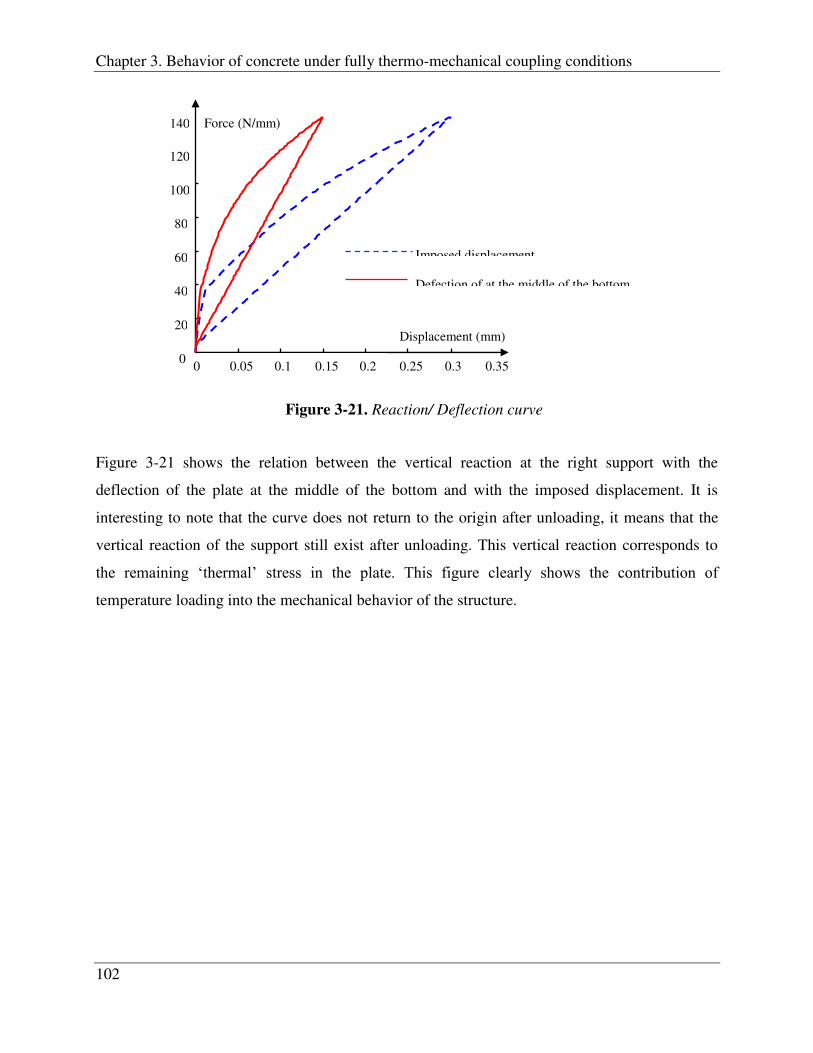
Chapter 3. Behavior of concrete under fully thermo-mechanical coupling conditions
102
Figure 3-21 shows the relation between the vertical reaction at the right support with the
deflection of the plate at the middle of the bottom and with the imposed displacement. It is
interesting to note that the curve does not return to the origin after unloading, it means that the
vertical reaction of the support still exist after unloading. This vertical reaction corresponds to
the remaining „thermal‟ stress in the plate. This figure clearly shows the contribution of
temperature loading into the mechanical behavior of the structure.
0 0.05 0.1 0.15 0.2 0.25 0.3 0.35 0
20
40
60
80
100
120
140
Displacement (mm)
Force (N/mm)
Imposed displacement
Defection of at the middle of the bottom
Figure 3-21. Reaction/ Deflection curve
Localized Failure for Coupled Thermo-Mechanics Problems
103
3.6 Conclusion
We have introduced in this chapter a new localized failure model with themo-damage coupling
for concrete material. The main contribution consists in the ability of the model to describe the
softening behavior of the material at localization failure zone, which is necessary to estimate the
load limitation of the structure under the fully thermo-mechanical loading. Both theoretical
formulation and solution procedure for the problem were carefully considered in order to make a
successful development. The theoretical formulation proved that there is a “jump” in heat flux
through the cracking surface when localized failure happens due to mechanical loading, which is
represented by a “jump” in displacement field. These “discontinuity” values of displacement and
heat flux were modeled in the framework of the embeded-discontinuity finite element method.
The solution procedure for the problem exploits the adiabatic operator split. This implies that the
problem is first solved for mechanical part (with adiabatic condition), and then for thermal part
(or heat transfer problem). The theoretical development and the numerical solution were carried
out for general two-dimensional problems. Three most general examples concerning the traction
test and the bending test were performed and discussed to illustrate the capabilities of the
proposed approach.
The received results illustrate the considerable effect of temperature loading on the mechanical
response of concrete structure. In particular, one can infer that the mechanical resistance of the
structure significantly reduces when it is subjected to thermal loading at the same time. On the
constrary, the mechanical loading also leads to the thermal response of the structure. Whereas,
the temperature of the concrete at damage and/or localized failure zone increases due to the
appearance of mechanical dissipation and structural heating.

Chapter 4. Thermomechanics failure of reinforced concrete frames
104
4 Thermomechanics failure of reinforced concrete frames
4.1 Introduction
In this chapter we present a new model for computing the nonlinear response of reinforced
concrete frames subjected to coupled thermomechanical loads. The first major novelty of the
model is its ability to account for both bending and shear failure of the reinforced concrete
frames. The second novelty concerns the model capability to represent the total degradation of
the material properties due to high temperature and the thermal deformations. These nouvelties
will be introduced in this chapter by the following sequence. In section 4.2, we studied the
degradation of mechanical resistance of the reinforced concrete cross-section under bending
moment, shear force and axial loading due to temperature increase. These degradations was
studied based on the „layer‟ method in the framework of Modified Compression Theory
proposed by Vecchio and Collins (see [41],[58],[59]) but was extended to include the
temperature dependence of material properties and the stress-strain condition due to thermal
loading. In this method, the cross-section is divided into layers, which are small enough to
assume uniform stress and strain condition and constant temperature in all over the layer. By
that way, the reduction of material properties due to temperature at each layer isconsidered and
accumulated into the degradation of overall resistance of the cross-section. The thermal strain
due to temperature gradient at each layer is also taken into account to estimate the total
deformation of the cross-section and to compute the total stress at each layer. The latter
contributes in total response of the section, especially for high temperature typical of fire
loading. In section 4.3, we introduce the finite element method to provide an efficient
computational frameworkusing the stress-resultant constitutive model of reinforced concrete
beam element. The latteris then used for limit load computations of the reinforced concrete frame
structures subjected to combined mechanical loading and fire. Several numerical examples will
be introduced and discussed in section 4.4 to prove the capablity of the proposed method.

Localized Failure for Coupled Thermo-Mechanics Problems
105
4.2 Stress-resultant model of a reinforced concrete beam element subjected to
mechanical and thermal loads.
4.2.1 Stress and strain condition at a position in reinforced concrete beam element under
mechanical and temperature loading.
Table 4-1. List of symbols for thermomechanical model
Symbol Meaning
θ Angle of principal direction (for both deformation and stress condition)
x Normal stress in x direction (longitudinal direction)
y Normal stress in y direction (tranverse direction)
Shear stress
1 1st (maximum) principal stress
2 2nd (minimum) principal stress
εxm Mechanical normal strain in x direction (longitudinal direction)
εym Mechanical normal strain in y direction (tranverse direction)
γ Shear strain
ε1 1st (maximum) principal strain
ε2 2nd (minimum) principal strain
xt Thermal stress in x direction (longitudinal direction)
yth Thermal stress in y direction (tranverse direction)
εxth Thermal strain in x direction (longitudinal direction)
Consider a reinforce concrete beam element subjected to mechanical loading and thermal loading
(see Figure 4-1)

Chapter 4. Thermomechanics failure of reinforced concrete frames
106
Figure 4-1. Mechanical loading and fire acting on reinforced concrete element
In this element, beside the mechanical deformation, a thermal strain is also acting. The total
strain is then the sum of mechanical strain and thermal strain:
thm (4-1)
Figure 4-2 represents the thermal stress and strain condition at a given point in the element.
0
Figure 4-2. Thermal stress and thermal strain condition
The thermal strain of concrete depends on the temperature and the kind of aggregates [7], such
that we have for calcareous aggregates
CTfor
CTCforTTTcth 03
0031164
8051012
80520104.1106102.1
(4-2)
for siliceous aggregates:
CTCfor
CTCforTTTcth 003
0031164
12007001014
70020103.2109108.1
(4-3)
The thermal strain of steel also depends on the temperature [7]:
łxth
łyth=0
Ńxth Ńxth
Ńyth=0
Ńyth=0 x
y
M
N V N V
M

Localized Failure for Coupled Thermo-Mechanics Problems
107
CTCforT
CTCfor
CTCforTT
stm
0053
003
002854
1200860102102.6
8607501011
75020104.0102.110416.2
(4-4)
Noted that we have assumed that the normal part of the thermal strain and thermal stress in the
transverse direction of the element is equal to zero (łyth=0 and Ńyth=0, see Figure 4-2). A similar
assumption also applies to mechanical stress and strain; in particular, the normal part of
mechanical stress and mechanical strain are also ignored ( 0y , 0y ). This assumption is
sometimes declared by „no interactive compression between longitudinal layers of the element‟
or „the depth of the cross-section is constant after loading‟, which is a well-known and widely
accepted hypothesis in beam analysis. Due to this assumption, only the longitudinal strain (łx)
and the shear strain ( ) are considered as non-zero strain components of the beam element (see
Figure 4-3).
The total stress and strain condition at a point in reinforced concrete beam element can be
represented by a Mohr circle (see Figure 4-4).
x x
y=0
y =0
v
v
θ
x
y
εx=εxm+εxth
γ
εy=0
Figure 4-3. Total stress and strain condition at a position in beam element (εy=0 and y=0)

Chapter 4. Thermomechanics failure of reinforced concrete frames
108
The angle giving the orientation of the principal directions can then be defined according to:
x
22tan
(4-5)
The maximum value of principal strain is:
22
22
1xx
(4-6)
The mimimum value of principal strain is:
22
22
2xx
(4-7)
We note that in this case, the maximum strain is always positive and the minimum strain is
always negative.
Once the strain components are known, we can compute the corresponding stress components by
using the constitutive equation between principal stress and principal strain (assuming that the
εy=0
2θ
εx
ε2 ε1
γ
γ
ε 2θ
x
y =0
1 2
Figure 4-4. Mohr circle representation for strain and stress condition at a point in beam
element

Localized Failure for Coupled Thermo-Mechanics Problems
109
principal directionsfor strain and stress are the same). The constitutive equation between
principal stress and principal strain of concrete and rebaris dependent on the temperature; it
canbe approximated by a number of mathematical equations (see [59],[7] ,[9],[11],[60], [61],
[55]). In the following, some typical relationships are introduced:
Concrete
The mechanical stress-strain constitutive equation for concrete in compression can be computed
by the following equation (see [10]) (see Figure 4-5):
TforT
TTf
TforT
TTf
mexc
c
c
c
c
c
c
2
max
max'
max
2
max
max2'
2
31
)(1
(4-8)
where 62max 1004.06025.0 TTT
The compressive strength of concrete is dependent on temperature [7]:
TCfor
CTCforTf
CTCforTf
CTforf
Tf
c
c
c
c
0
00'
00'
0'
'
9000
9004000016.044.1
40010000067.0067.1
100
(4-9)
where 'cf is the compressive strength of concrete at room temperature (200C)

Chapter 4. Thermomechanics failure of reinforced concrete frames
110
Figure 4-5. Relation between compressive stress and strain of concrete due to tempeture[10]
The negative principal stress of concrete can also be computed from the negative principal strain
by the equations of Vecchio and Collins (see [61]), which are widely used in American building
codes (see[9], [12]). In which, the minimum principal stress is computed by the equation:
2
'2
'2
22 2max
c
c
c
c
cc
(4-10)
where
''
'1
2
34.08.0
1max cc
c
c
c ff
(4-11)
The principal stress-strain relation of concrete in tension can be computed by following the
suggestion of Vecchio and Collins (see [61]):
0
0.2
0.4
0.6
0.8
1
1.2
0 0.02 0.04 0.06 0.08
Str
ess
/ Com
pres
sive
str
engt
h
Strain
T=20 C
T=200 C
T=400 C
T=600 C
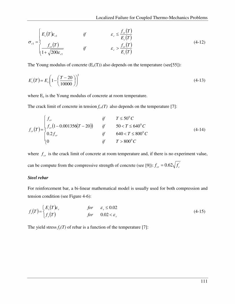
Localized Failure for Coupled Thermo-Mechanics Problems
111
TE
Tfif
Tf
TE
TfifTE
c
cr
c
c
cr
c
cr
ccc
c
1
1
1
2001
(4-12)
The Young modulus of concrete (Ec(T)) also depends on the temperature (see[55]):
2
'
10000
201
T
ETE cc
(4-13)
where Ec is the Young modulus of concrete at room temperature.
The crack limit of concrete in tension fcr(T) also depends on the temperature [7]:
CTif
CTiff
CTifTf
CTiff
Tf
cr
cr
cr
cr
0
0
0
0
8000
8006402.0
6405020001356.01
50
(4-14)
where crf is the crack limit of concrete at room temperature and, if there is no experiment value,
can be compute from the compressive strength of concrete (see [9]): '62.0 ccr ff
Steel rebar
For reinforcement bar, a bi-linear mathematical model is usually used for both compression and
tension condition (see Figure 4-6):
sy
sss
sforTf
forTETf
02.0
02.0
(4-15)
The yield stress fy(T) of rebar is a function of the temperature [7]:
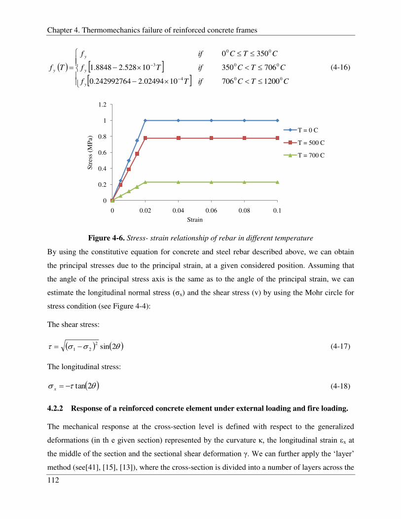
Chapter 4. Thermomechanics failure of reinforced concrete frames
112
CTCifTf
CTCifTf
CTCiff
Tf
y
y
y
y
004
003
00
12007061002494.2242992764.0
70635010528.28848.1
3500
(4-16)
Figure 4-6. Stress- strain relationship of rebar in different temperature
By using the constitutive equation for concrete and steel rebar described above, we can obtain
the principal stresses due to the principal strain, at a given considered position. Assuming that
the angle of the principal stress axis is the same as to the angle of the principal strain, we can
estimate the longitudinal normal stress (Ńx) and the shear stress (v) by using the Mohr circle for
stress condition (see Figure 4-4):
The shear stress:
2sin221 (4-17)
The longitudinal stress:
2tanx (4-18)
4.2.2 Response of a reinforced concrete element under external loading and fire loading.
The mechanical response at the cross-section level is defined with respect to the generalized
deformations (in th e given section) represented by the curvature , the longitudinal strain łx at
the middle of the section and the sectional shear deformation . We can further apply the „layer‟
method (see[41], [15], [13]), where the cross-section is divided into a number of layers across the
0
0.2
0.4
0.6
0.8
1
1.2
0 0.02 0.04 0.06 0.08 0.1
Stre
ss (
MP
a)
Strain
T = 0 C
T = 500 C
T = 700 C

Localized Failure for Coupled Thermo-Mechanics Problems
113
beam depth. Each layer is assumed to be thin enough to allow for uniform distributions of stress,
strain and temperature (see Figure 4-7).
We denote the layer width and height as bci and hci, the longitudinal stress as cxi and the distance
from the middle of the layer to the top of the cross-section of concrete layer „ith‟ as yci;
furthermore, we denote the steel bar areasxja , the longitudinal stress sxj and the distance from the
middle of the rebar element to the top of the cross section of the rebar element „jth‟ as ysj, we can
establish the following set of equilibrium equations:
Ńcx Ńsx
Mu
Nu
Axial Force and Moment Concrete layer and Rebar
yci
ysj
1
y
łxm
Temperature Gradient
T
łxth
Shear Force
Vu
Parabol shear strain distribution
ń
Figure 4-7. Response of reinforced concrete element under mechanical and thermal loads
Chapter 4. Thermomechanics failure of reinforced concrete frames
114
c
sc
c
N
i
iii
N
j
sjsxjsxj
N
i
cicicicxi
N
i
Ns
j
sxjsxjcicicxi
Vhb
Myyayyhb
Nahb
1
11
1 1
(4-19)
where y is the distance from the neutral axis (where 0x ) to the top of the cross-section.
This system allows us to compute the response of the cross-section, and in particular curvature,
longitudinal strain and shear deformation, at a given force and temperature loads; the following
procedure is used (see Figure 4-8):

Localized Failure for Coupled Thermo-Mechanics Problems
115
NO: Adjust y and κ
OK
OK
Compute longitudinal strain distribution ( test
xi ) from assuming curvature test and position
of neutral axis ( testy ) with plane section hypothesis (figure 7)
Estimate the stress condition ( ,, 21 ii ) of each layer from the strain condition ( ,, 21 ii )
by the principal stress-strain contitutive equation (8 to 16). Compute the longitudinal stress ( test
xi ) and the shear stress ( test
iv ) for each layer (equation 17 and 18)
Compute resulting internal force:
cN
i
Ns
j
sxj
test
sxicici
test
cxi ahbN1 1
sc N
j
test
sjsxj
test
sxj
N
i
test
cicici
test
cxi yyayyhbM11
; cN
i
ii
test
i hbV1
Check: N= Nu and M = Mu
END
Compute temperature distribution along the cross-section: Tci; Tsj
Specific section mechanical loading: Mu, Nu, Vu
Assume parabol shear strain distribution: max (figure 7)
Estimate the strain condition ( ,, 21 ii ) at layer „ith‟ from test
xi , test
i and with the
assumption that 0y (depth of the layer remains the same after loading)
Check: V = Vu NO: Adjust xy
Figure 4-8. Procedure to determine the mechanical response of RC beam element

Chapter 4. Thermomechanics failure of reinforced concrete frames
116
4.2.3 Effect of temperature loading, axial force and shear load on mechanical moment-
curvature response of reinforced concrete beam element.
By applying the procedure illustrated inFigure 4-8, we can establish the moment-curvature
relation for a reinforced concrete beam element, by fixing the temperature loading, the shear
loading, the axial force and tracking the increase of the internal moment (M) proportional to the
increase of the curvature (κ).
Figure 4-11shows the degradation of the moment-curvature response of a rectangular reinforced
concrete beam exposed to ASTM 119 fire acting on the bottom (see Figure 4-9) in case external
axial force and shear force equals to zero (pure bending test) (Nu = 0, Vu =0). The temperature
profile of the RC beam subjected to fire loading increases due to time (Figure 4-10-[11]).When
temperature increases, the strength of materials (concrete and rebar) decreases and leads to the
degradation of moment-curvature resistance of the element.
Figure 4-9. Cross-section and Dimensioning of the consider reinforced concrete element
Figure 4-10. Evolution of temperature profile due to time[11]
150 150
300mm 500m
3D20
2D14
D10
0100200300400500600700800900
1000
0 100 200 300 400 500
Tem
pera
ture
(oC
)
Distance to bottom of the beam (mm)
t=1h
t=2h
t=3h

Localized Failure for Coupled Thermo-Mechanics Problems
117
Figure 4-11. Dependence of moment-curvature with time exposure to fire ASTM119
Figure 4-12 illustrates the evolution of bending resistance of the frame with an increase of the
axial compression.
Figure 4-12. Dependence of moment-curvature on axial compression
Figure 4-13 expresses the reduction of the bending resistance when shear load increases at four
instants: t =0h, t=1h, t=2h and t=3h.
0
20
40
60
80
100
120
140
160
180
200
0 0.05 0.1 0.15 0.2
Mom
ent (
kN.m
)
Curvature (1/m)
t=0h
t=1h
t=2h
0
50
100
150
200
250
300
0 0.05 0.1 0.15 0.2
Mom
ent (
kN/m
)
Curvature (1/m)
N=0kN
N=100 kN
N=500kN

Chapter 4. Thermomechanics failure of reinforced concrete frames
118
Figure 4-13. Dependence of moment-curvature response on shear loading
From Figure 4-11 to Figure 4-13, we have indicated that the moment-curvature curve can
approximately be represented by a multi-linear curve (see [62]) with the „crack‟ moment εc, the
„yield‟ moment My, the „ultimate‟ moment εu and the corresponding values of curvature: c ,
y , u . The „crack‟ moment is obtained at the state where the tensile fiber of concrete starts to
crack. The „yield‟ moment is the moment acting on the cross section to make the tensile rebar
starts to yield. The peak resistance of the beam is reached when both the tensile rebar yields and
the concrete the compressive fiber collapses to make the „ultimate‟ bearing state of the beam.
From this state on, the „bending hinge‟ occurs at the cross-section and the bending resistance of
the cross-section starts to decrease with further curvature increase (see Figure 4-14).
020406080
100120140160180200
0 0.05 0.1 0.15 0.2
Mom
ent (
kN.m
)
Curvature (1/m)
t=0h,V=0kN
t=0h,V=50kN
t=0h,V=100kN
020406080
100120140160180200
0 0.05 0.1 0.15 0.2
Mom
ent (
kN.m
)
Curvature (1/m)
t=1h,V=0kN
t=1h,V=50kN
t=1h,V=100kN
0
20
40
60
80
100
120
140
160
180
0 0.05 0.1 0.15 0.2
Mom
ent (
kN.m
)
Curvature (1/m)
t=2h,V=0kN
t=2h,V=50kN
t=2h,V=100kN
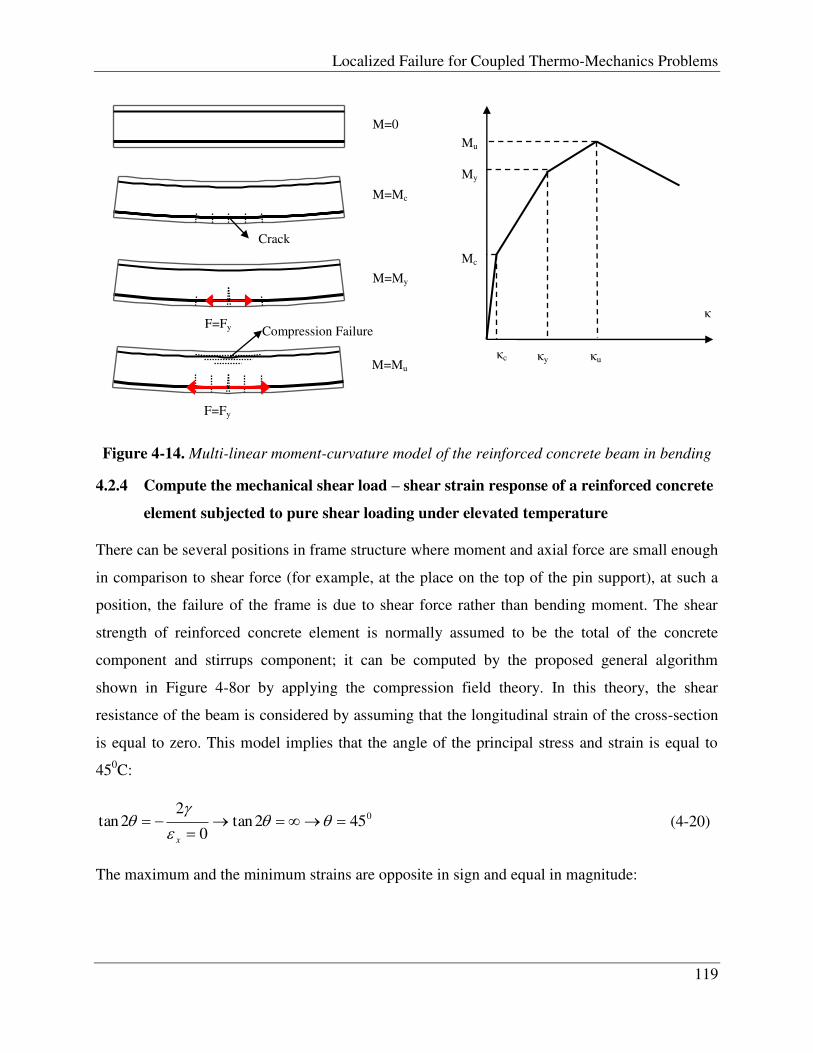
Localized Failure for Coupled Thermo-Mechanics Problems
119
Figure 4-14. Multi-linear moment-curvature model of the reinforced concrete beam in bending
4.2.4 Compute the mechanical shear load – shear strain response of a reinforced concrete
element subjected to pure shear loading under elevated temperature
There can be several positions in frame structure where moment and axial force are small enough
in comparison to shear force (for example, at the place on the top of the pin support), at such a
position, the failure of the frame is due to shear force rather than bending moment. The shear
strength of reinforced concrete element is normally assumed to be the total of the concrete
component and stirrups component; it can be computed by the proposed general algorithm
shown in Figure 4-8or by applying the compression field theory. In this theory, the shear
resistance of the beam is considered by assuming that the longitudinal strain of the cross-section
is equal to zero. This model implies that the angle of the principal stress and strain is equal to
450C:
0452tan0
22tan
x
(4-20)
The maximum and the minimum strains are opposite in sign and equal in magnitude:
u y c
Mc
My
Mu
M=0
M=Mc
M=My
M=Mu
F=Fy
F=Fy Compression Failure
Crack

Chapter 4. Thermomechanics failure of reinforced concrete frames
120
12
2
1 2
0
2
0 xx
(4-21)
22
2
2 2
0
2
0 xx
(4-22)
The principal stress can be computed from principal strain for concrete and steel bar by applying
equations from equation (4-8) to equation (4-16). The shear stress therefore can be computed
from the shear strain and the temperature at each concrete layer and/or rebar element:
iiimimii TfTfv ,,11 (4-23)
Figure 4-15. Stress components of reinforced concrete subjected to pure shear loading
The equilibrium equation for shear force:
svsvcici
N
i
ciscu As
dcotanhbvVVV
c 1 (4-24)
Where d is the „effective‟ depth of reinforced concrete cross section subjected to shear load, s is
the stirrups‟ spacing, Asv is the area of stirrup and sv is the stress in the stirrups corresponding
to the considered shear strain. For pure shear test ( 045 ), equation (4-24) becomes:
θ
vci
Layer i
Layer i-1
Layer i+1
Ń1ci
Ńysk
Ńysk
d
dcotan(θ)
Vu
Stress condition Stress condition in concrete Stress condition in stirrups
s

Localized Failure for Coupled Thermo-Mechanics Problems
121
svsvcici
N
i
ciscu As
dhbVVV
c 1 (4-25)
From the equation (4-23) to (4-25), we can estimate the corresponding shear force (Vu) of a
given shear deformation ( ), which allows us to draw the shear force–shear strain diagram in a
given cross-section.
Figure 4-16 shows the reduction of shear resistance of the RC element given in Figure 4-9when
subjected to fire ASTM119.
Figure 4-16. Mechanical shear force- shear deformation diagram
With a similar approximation already usedfor the moment-curvature curve, we also introduce a
multi-linearresponse forthe shear resistance of a reinforced concrete element (see Figure 3-16 for
illustration). In the next section, we show how to apply these stress-resultant models inthe finite
element analysis of reinforced concrete frame structure subjected to combined mechanical and
thermal loads, by using the Timoshenko beam element.
0
50
100
150
200
250
300
350
400
450
500
0.00% 0.01% 0.02% 0.03% 0.04%
Sh
ear
Fo
rce
(kN
)
Shear Deformation
t=0h
t=1h
t=2h
t=3h

Chapter 4. Thermomechanics failure of reinforced concrete frames
122
4.3 Finite element analysis of reinforced concrete frame
4.3.1 Timoshenko beam with strong discontinuities
Figure 4-17. Beam under external loading and fire
We consider a straight Timoshenko beam of length land cross-section A. The beam is submitted
to distributed axial load f(x), transverse load q(x), bending moment m(x), the concentrated forces
F, Q and C. The beam is also exposed to fire loading. We denote as Γu and Γq the set of points in
(0,l) where displacements and forces are prescribed, respectively (seeFigure 4-17). We consider
a point x, lx ,0 , on the beam neutral axis, and denote as xxvxux ,,u the
generalized displacements (namely the longitudinal displacement, transverse displacement and
rotation) at that point. With such a notation, the generalized strains at point xare obtained by
taking into account the standard Timoshenko beam formulations:
xx
xx
vx
x
ux
x
ε
(4-26)
Denoting as N, V and M respectively the axial force, transverse shear force and bending
moment, the strong form of the local equilibrium can be written as:
Q C
F Γu
f(x) Γq
q(x) m(x)

Localized Failure for Coupled Thermo-Mechanics Problems
123
0
0
0
xmxTx
M
xqx
V
xfx
N
(4-27)
The corresponding weak form for the standard Timoshenko beam model can then be written as:
lT
lTT
FdxBfdx0 0
wwσ
(4-28)
Where σ is the stress-resultant vector ( TMVNσ ), w is a virtual generalized
displacement ( 0Vw where uonandlHRlV 0,0,0: 130 www ), Tmqf ,,f is
the vector of distributed load TCQF ,,F the vector of concentrated forces.
In order to represent the development of localized failure mechanism or „plastic hinge‟ in a
reinforced concrete beam, we consider discontinuity in the generalized displacement field at a
particular point xc of the neutral-axis. Indeed, a plastic hinge that is no more than a narrow zone
where plastic behavior concentrates leading to a very localized dissipation, at the scale of the
beam, can simply be interpreted as a discontinuity of the generalized displacement field. In that
case, the generalized displacement u is now decomposed into a regular part and a discontinuous
part as:
cc xv
u
x
x
xv
xu
xx
αuu
(4-29)
where ,, vuα is the displacement jump at point cx and cx is the Heaviside function
defined by 0 xcx
for cxx and 1 xcx
for cxx . A graphic illustration of the beam
kinematics is presented inFigure 4-18.
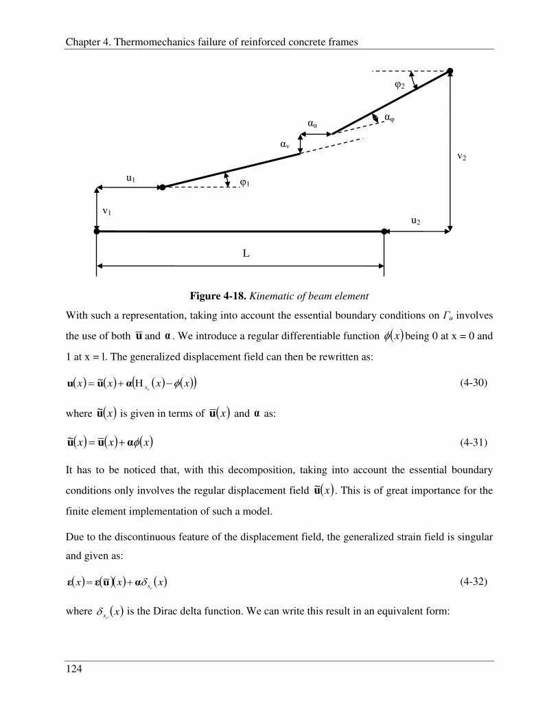
Chapter 4. Thermomechanics failure of reinforced concrete frames
124
Figure 4-18. Kinematic of beam element
With such a representation, taking into account the essential boundary conditions on Γu involves
the use of both u and α . We introduce a regular differentiable function x being 0 at x = 0 and
1 at x = l. The generalized displacement field can then be rewritten as:
xxxxcx αuu ~
(4-30)
where xu~ is given in terms of xu and α as:
xxx αuu ~ (4-31)
It has to be noticed that, with this decomposition, taking into account the essential boundary
conditions only involves the regular displacement field xu~ . This is of great importance for the
finite element implementation of such a model.
Due to the discontinuous feature of the displacement field, the generalized strain field is singular
and given as:
xxxcxαuεε
(4-32)
where xcx is the Dirac delta function. We can write this result in an equivalent form:
L
u1
v1
Ņ1
Ņ2
v2
u2
αv
αu αŅ

Localized Failure for Coupled Thermo-Mechanics Problems
125
xxxxcxααGuεε ~
(4-33)
where G is equal to xL , L being the displacement-to-strain operator.
Practically, there is no need to define precisely the function x , only its derivative is needed.
Indeed, in the finite element implementation, the interpolation of displacement is considered in
its standard form whereas the strain field is locally enriched in each finite element to take into
account the influence of a displacement discontinuity. This point is discussed in the next section.
4.3.2 Stress-resultant constitutive model for reinforced concrete element
In this article, the stress-resultant models are used to describe the behavior of reinforced concrete
beam element. Two different failure modes are considered here: one is related to bending failure
giving rise to a rotation discontinuity (or bending „hinge‟) and the other one is related to shear
failure accompanied by a vertical displacement discontinuity (or shear „hinge‟) (see[20],[19]).
For both models, a plasticity-type formulation is chosen.
4.3.2.1 Model for bending failure
Relaying upon the generalized procedure for the classical plasticity (see [17]), we consider the
following main modeling gradients:
• additive decomposition of the curvatureμ
pe (4-34)
where e denotes the elastic part of the curvature and p denotes the plastic part of the
curvature.
• Helmholtz free energyμ
eeeEI
2
1,
(4-35)
where E is the homogenized Young modulus of the reinforced concrete beam, I is the cross-
section inertia and Ξ is the hardening potential written in terms of the hardening variable ξ.
• yield functionμ

Chapter 4. Thermomechanics failure of reinforced concrete frames
126
qMMqM y ,
(4-36)
where yM demotes the elastic limit moment, qis the stress-like variable associated to the
hardening variable ξ.
The use of the second principle of thermodynamics for elastic case provides constitutive
equations:
KIqEIEIMep ; (4-37)
where we have considered a linear hardening law with KI the hardening parameter. Moreover, by
considering the principle of maximum plastic dissipation, the evolution law and constitutive
equations are obtained as:
q
MsignM
p ;
(4-38)
and
0
0
KIEI
EIKI
EI
M
(4-39)
along with the loading/unloading conditions 0,0,0 and consistency condition
0 .
Due to the activation of different dissipative (irreversible) mechanisms in the materials that
constitute the reinforced concrete, different stages of the bulk behavior have to be reproduced.
To that end, we consider two different subsequent yield functions of the type presented in
equation (4-36) to describe the bulk hardening part for bending response (see Figure 4-19).
Those two functions are characterized by different limit values and hardening parameters:
• the first yield function is used to describe the behavior when the first cracks occur in concrete,
with nonlinearities and dissipation appearing in the beam:

Localized Failure for Coupled Thermo-Mechanics Problems
127
cccc qMMqM ,
(4-40)
where Mc corresponds to the elastic limit of the beam (when first concrete crack appears) and
IKqc 1 is the stress-like variable associated to hardening with K1I the hardening parameter;
• the second phase is characterized by the yielding of steel rebars. The corresponding yield
function is given by:
yyyy qMMqM ,
(4-41)
where My denotes the bending moment corresponding to the yielding of steel rebar and
IKq yy with K2Ithe hardening parameter.
The softening part of the behavior is controlled by the following yield condition:
0, qMMqM uxx cc (4-42)
where Mxc denotes the bending moment on the discontinuity at xc, Mu is the ultimate bending
moment value and q is the stress-like variable associated to softening. Here again, as for the
bulk, we consider a linear softening, so that we have: IKq with 0K .
It has to be noticed here that, due to the rigid behavior of the plastic hinge at xc, the equivalent
total strain αθ and the plastic strain are equal. αθis then interpreted as a plastic strain and its
evolution is given by:
q
andMsignM
(4-43)
where is the plastic multiplier associated to the plastic hinge behavior. The constitutive
equation is then given by:
IKMcx
(4-44)
A representation of the bulk and discontinuity behavior is given inFigure 4-19, which is similar
to what had been explained inFigure 4-14, expect the fact that the softening behavior of the
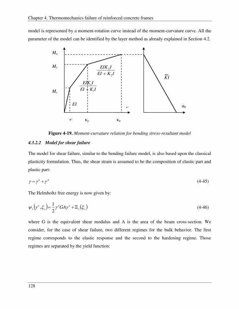
Chapter 4. Thermomechanics failure of reinforced concrete frames
128
model is represented by a moment-rotation curve instead of the moment-curvature curve. All the
parameter of the model can be identified by the layer method as already explained in Section 4.2.
Figure 4-19. Moment-curvature relation for bending stress-resultant model
4.3.2.2 Model for shear failure
The model for shear failure, similar to the bending failure model, is also based upon the classical
plasticity formulation. Thus, the shear strain is assumed to be the composition of elastic part and
plastic part:
pe (4-45)
The Helmholtz free energy is now given by:
vv
ee
v
e
v GA 2
1,
(4-46)
where G is the equivalent shear modulus and A is the area of the beam cross-section. We
consider, for the case of shear failure, two different regimes for the bulk behavior. The first
regime corresponds to the elastic response and the second to the hardening regime. Those
regimes are separated by the yield function:
EI
IKEI
IEIK
1
1
IKEI
IEIK
2
2
Mc
My
Mu
c y u
αθ
IK

Localized Failure for Coupled Thermo-Mechanics Problems
129
0, vyvv qVVqV (4-47)
where yV denotes the elastic limit,
vq denotes the stress-like variable which controls the yield
limit: vvv AKq
The state equations, evolution equations and constitutive equations are now of the following
form:
epGAGAV (4-48)
and
v
v
vvvv
vv
p
qandVsign
V
(4-49)
0
0
v
v
v
v
AKGA
AGAK
GA
V
(4-50)
As regards to the plastic hinge in shear, the same kind of modification as the one already
presented for the bending failure is introduced but with respect to vertical displacement
discontinuity. The corresponding yield function is now given by:
0, vuxvx qVVqVcc
(4-51)
where cxV denotes the shear load at the discontinuity point xc, Vuis the ultimate shear load value
and finally vq denotes the stress-like variable thermodynamically conjugate to the softening
variable v : vvv AKq (if we consider linear softening). The shear hinge model is also rigid-
plastic, and the displacement discontinuity v is interpreted as an equivalent plastic strain.
Hence, the corresponding constitutive equation for softening response in shear failure can be
written as:
vvx AKVc
(4-52)
A representation of the shear behavior (bulk and discontinuity) is given inFigure 4-20.

Chapter 4. Thermomechanics failure of reinforced concrete frames
130
Figure 4-20. Shear load-shear strain relation for shear stress-resultant model
4.3.3 Finite element formulation
4.3.3.1 Finite Element interpolations and global resolution
The finite element implementation of the model presented herein is based upon the incompatible
mode method (see [18]). The use of such a technique ensures that the enrichment with a
generalized displacement jump remains local, and that no additional degrees of freedom are
required at the global level of the solution the procedure. We present subsequently the key points
of the finite element implementation and the added interpolation shape functions used in our
case.
We consider a standard two-node Timoshenko beam finite element. The classical interpolation
for such an element is then given by:
Ndu
2211
2211
2211
xNxNx
vxNvxNxv
uxNuxNxu
xh
h
h
h
(4-53)
where
AKv
V
GA
V
Vu
αv γ
Vy
Vu
AKGA
AGAK
v
v
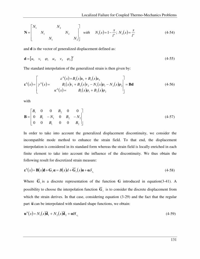
Localized Failure for Coupled Thermo-Mechanics Problems
131
ee
l
xxN
l
xxNwith
NN
NN
NN
21
21
21
21
;1N
(4-54)
and d is the vector of generalized displacement defined as:
Tvuvu 222111 d (4-55)
The standard interpolation of the generalized strain is then given by:
Bdε
2211
22112211
2211
xBxBx
xNxNvxBvxBx
uxBuxBx
xh
h
h
h
(4-56)
with
21
2211
21
0000
00
0000
BB
NBNB
BB
B
(4-57)
In order to take into account the generalized displacement discontinuity, we consider the
incompatible mode method to enhance the strain field. To that end, the displacement
interpolation is considered in its standard form whereas the strain field is locally enriched in each
finite element to take into account the influence of the discontinuity. We thus obtain the
following result for discretized strain measure:
cxrr
hxdxBxx ααGαGdBε
(4-58)
Where rG is a discrete representation of the function G introduced in equation(3-41). A
possibility to choose the interpolation function rG is to consider the discrete displacement from
which the strain derives. In that case, considering equation (3-29) and the fact that the regular
part u can be interpolated with standard shape functions, we obtain:
cx
hHxNxNx αddu 2211
(4-59)

Chapter 4. Thermomechanics failure of reinforced concrete frames
132
Where id is the vector of nodal regular part of generalized displacement for node i. Due to the
properties of the interpolation functions and of the Heaviside function cxH , we obtain for the
total nodal displacements at node 1 in position x1 and at node 2 in position x2:
111 ddu xh and αddu 222x
h
(4-60)
so that the expression in (4-59) can be rewritten as:
xxNxNxcx
h ααddu 2211 (4-61)
xNxxNxNxcx
h
22211 αddu
(4-62)
We choose then for function x in (4-30), the function xN2 being 1C and equal to 0 at x1 and
to 1 at x2. With such a choice, the function rG is given by:
2
2
2
00
00
00
B
B
B
xrG
(4-63)
To build the weak form of the equilibrium equation, we consider the Hu-Washizu three-field
principle as usually done for incompatible mode method.
To that end, we use the same kind of interpolations for the virtual strain field * :
cxvv xxxxx ****** ββGdBβGdBε
(4-64)
where *d and *β denote the virtual nodal generalized displacement and virtual displacement
jump, respectively. With such interpolations, the weak form introduced in (4-28) leads to a set of
two equations that can be placed within the framework of incompatible mode method:
elemx
lT
V
lT
l
Nedx
dxdxd
c
e
,10,
0
*
*
0
*
0*
σGβ
FdfNdσBd T*
(4-65)
Considering the standard finite element assembly procedure, we obtain:

Localized Failure for Coupled Thermo-Mechanics Problems
133
elemx
lT
V
e
exteeN
e
Nedx
A
c
e
elem
,10
0
0
,int,
1
σσGh
ff
(4-66)
Where
eledx
0
int, σBf T , FfNf T elextedx
0
,
(4-67)
The first equation is the standard weak form of the equilibrium equation written concerning the
whole structure. The second equation, on the contrary, is local and written independently in each
element where a discontinuity has been introduced ( elemN denotes the set of elements enriched
with a discontinuity). cx
σ represents the value of the stress-resultant vector at point xc where the
discontinuity is introduced, this term arises in the equation due to the singularity of virtual strain
field (c
e
c x
l
x dx σσ 0 ). This second equation can be interpreted as the weak form of the stress-
resultant continuity across the localized failure point.
Remark: Function Gv is chosen, as suggested in the modified version of incompatible mode
method [18], in order to ensure the patch test, namely the verification of the second equation in
equation (4-66) for constant stress-resultant σ. We obtain then:
el
r
e
rv dxxl
xx0
1GGG
(4-68)
which gives in our case (Timoshenko beam element with only one integration point):
xx rv GG
4.3.3.2 Local resolution
Denoting as ithe iteration for time step n+1 of ζewton‟s iterative procedure, providing the
corresponding iterative updates i
n
i
n
i
n 1111 ddd and i
n
i
n
i
n 1111 ααα , the linearized
version of equation (4-66) is given by:
011,
,111,
,1,
,1
int,1
,1
11
,1,1
,1
1
i
n
i
n
ie
n
i
n
i
nd
ie
nv
ie
n
ie
n
exte
n
N
e
i
n
ie
nr
i
n
ie
n
N
eAA
elmelm
αKHdKFh
ffαFdK
(4-69)

Chapter 4. Thermomechanics failure of reinforced concrete frames
134
Here, we have adopted the following notations:
el ian
n
Tie
n dx0
,1
,1 BCBK ; el
r
ian
n
Tie
nr dx0
,1
,1, GCBF (4-70)
el ian
n
T
V
ie
n dx0
,1
,1 BCGF ; el
r
ian
n
T
V
ie
n dx0
,1
,1 GCGH (4-71)
where in 1, dK and i
n 1, αK are the consistent tangent stiffness for the discontinuity:
in
i
n
i
n
i
nd
i
nxc11,11,1, αKdKσ
(4-72)
and ian
n
,1C denotes the consistent tangent modulus for the bulk material obtained as a discretized
version of the tangent modulus given in equation (4-39) and equation (4-50):
in
ian
n
i
n 1,11 εCσ (4-73)
with σ and ε the generalized stress and strain, respectively.
The solution of the set of two equations in equation system (4-69) is obtained by taking
advantage of the local nature of the second equation, and the fact that it can be solved
independently in each localized element. For that purpose an operator splitting technique is used.
First, for a given nodal displacement increment in 1d at iteration I of the global Newton
procedure, the increment of displacement jump in 1α is sought by iterating in each localized
element upon the local equation 0,1 ie
nh (see equation (4-69)b). At the end of the local solution,
we then perform the static condensation at the element level, and carry on to solve the global part
of the Finite Element equilibrium equations:
ie
n
exte
n
N
e
i
n
ie
n
N
eAAelemelem
,int1
,1
11
,1
1
ˆ ffdK
(4-74)
where
i
nd
ie
nv
i
n
ie
n
ie
nr
ie
n
ie
n 1,,
1,
1
1,,
1,
1,,
1,
1ˆ
KFKHFKK
(4-75)
is the element tangent stiffness modified by the static condensation.
Localized Failure for Coupled Thermo-Mechanics Problems
135
We note in passing that the yield functions used in this work are totally uncoupled, so that the
vector equation in equation (4-66)b can be treated as a collection of corresponding scalar
equations. In the following, we present the resolution of such a scalar equation in a general form
without specifying the superscript M or V related to, respectively, bending or shear.
As already mentioned, the behavior on the discontinuity is rigid-plastic. Indeed, the displacement
jump is no more than a plastic displacement at discontinuity, with no elastic part contributing to
the displacement jump. Dueto this feature, it is not possible to compute trial tractions tr
xc
σ as
usuallydone for return-mapping algorithm (cx
σ denotes either cxM or
cxV ).
We have chosen here to use the local equilibrium equation (4-66b) to compute the trial tractions
values for a given set of nodal displacements in 1d . For a one point integration Timoshenko beam
element, this local equation is very simple and reduces to the strong form of the traction
continuity across the localized failure point; that is: ,dσσ cx
where ,dσ is the
corresponding generalized stress computed in the bulk. Moreover, we note that the activation of
the discontinuity is accompanied with softening, which involves elastic unloading of the bulk so
that the bulk and discontinuity internal variables cannot evolve simultaneously.
With this remarks in hand, the sketch of the algorithm can be given as follows:
• first compute the trial traction value by using equation (4-66b) and considering no evolution of
the internal variables: α, .
nnnn 11 , (4-76)
thus obtain the corresponding trial values of stress resultants:
p
n
tr
nr
i
n
etr
n
tr
nxcεαGBdCσσ 1111,
(4-77)
• then check the value of yield function tr
n
tr
nx
tr
n qc 11,1 , σ at discontinuity.
– if 01 trn , the trial state is admissible, no evolution of the internal variables is needed. In that
case, the consistent tangent stiffness for the discontinuity (see equation (4-72)) is such that:
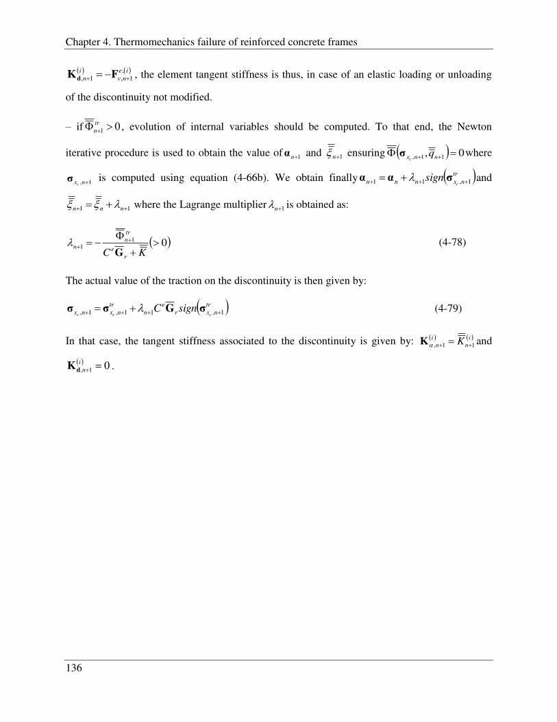
Chapter 4. Thermomechanics failure of reinforced concrete frames
136
ie
nv
i
n
,1,1, FKd , the element tangent stiffness is thus, in case of an elastic loading or unloading
of the discontinuity not modified.
– if 01 trn , evolution of internal variables should be computed. To that end, the Newton
iterative procedure is used to obtain the value of 1nα and 1n ensuring 0, 11, nnx qc
σ where
1, nxcσ is computed using equation (4-66b). We obtain finally tr
nxnnn csign 1,11 σαα and
11 nnn where the Lagrange multiplier 1n is obtained as:
011
KC r
e
tr
nn
G
(4-78)
The actual value of the traction on the discontinuity is then given by:
tr
nxr
e
n
tr
nxnx cccsignC 1,11,1, σGσσ
(4-79)
In that case, the tangent stiffness associated to the discontinuity is given by: in
i
n K 11, K and
01, i
ndK .
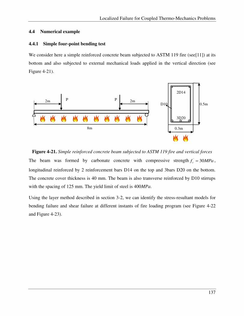
Localized Failure for Coupled Thermo-Mechanics Problems
137
4.4 Numerical example
4.4.1 Simple four-point bending test
We consider here a simple reinforced concrete beam subjected to ASTM 119 fire (see[11]) at its
bottom and also subjected to external mechanical loads applied in the vertical direction (see
Figure 4-21).
Figure 4-21. Simple reinforced concrete beam subjected to ASTM 119 fire and vertical forces
The beam was formed by carbonate concrete with compressive strength MPafc 30' ,
longitudinal reinforced by 2 reinforcement bars D14 on the top and 3bars D20 on the bottom.
The concrete cover thickness is 40 mm. The beam is also transverse reinforced by D10 stirrups
with the spacing of 125 mm. The yield limit of steel is 400MPa.
Using the layer method described in section 3-2, we can identify the stress-resultant models for
bending failure and shear failure at different instants of fire loading program (see Figure 4-22
and Figure 4-23).
0.3m
0.5m
3D20
2D14
D10
8m
P P 2m 2m

Chapter 4. Thermomechanics failure of reinforced concrete frames
138
Figure 4-22. Reduction of bending resistance due to time exposing to fire ASTM 119
The corresponding values of material parameters for bending model are given inTable 4-2.
Table 4-2. Bending model parameters for different instants of fire loading program
Parameters t =0h t =1h t =2h t=3h
Young Modulus (kN/m2) 2708121 2835722 2644230 1324882
Hardening Modulus K1 (kN/m2) 795440.3 773984.9 540969.6 279660.4
Hardening Modulus K2(kN/m2) 433372.2 404203.2 99201.84 177893.4
Softening Modulus K (kN/m) -66943.8 -34230.2 -79727.8 -40232.5
Crack shear Mc (kN) 42.3144 44.30815 41.3161 41.40257
Yield shear My (kN) 87.15347 177.3368 134.2953 76.36012
Ultimate shear Mu (kN) 192.5736 189.9682 137.3953 81.91929
0
50
100
150
200
250
0 0.02 0.04 0.06 0.08
Mom
ent (
kN.m
)
Curvature (1/m)
t=0h
t=1h
t=2h
t=3h
0
50
100
150
200
250
0 0.02 0.04
αŅ (rad)
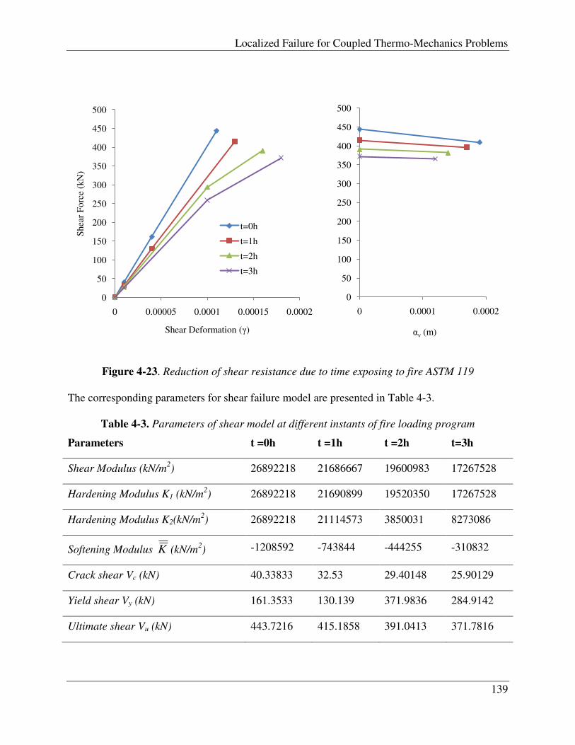
Localized Failure for Coupled Thermo-Mechanics Problems
139
Figure 4-23. Reduction of shear resistance due to time exposing to fire ASTM 119
The corresponding parameters for shear failure model are presented in Table 4-3.
Table 4-3. Parameters of shear model at different instants of fire loading program
Parameters t =0h t =1h t =2h t=3h
Shear Modulus (kN/m2) 26892218 21686667 19600983 17267528
Hardening Modulus K1 (kN/m2) 26892218 21690899 19520350 17267528
Hardening Modulus K2(kN/m2) 26892218 21114573 3850031 8273086
Softening Modulus K (kN/m2) -1208592 -743844 -444255 -310832
Crack shear Vc (kN) 40.33833 32.53 29.40148 25.90129
Yield shear Vy (kN) 161.3533 130.139 371.9836 284.9142
Ultimate shear Vu (kN) 443.7216 415.1858 391.0413 371.7816
0
50
100
150
200
250
300
350
400
450
500
0 0.00005 0.0001 0.00015 0.0002
She
ar F
orce
(kN
)
Shear Deformation ( )
t=0h
t=1h
t=2h
t=3h
0
50
100
150
200
250
300
350
400
450
500
0 0.0001 0.0002
αv (m)
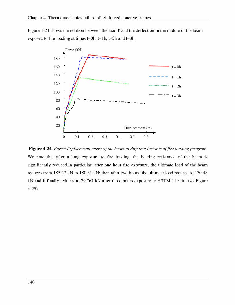
Chapter 4. Thermomechanics failure of reinforced concrete frames
140
Figure 4-24 shows the relation between the load P and the deflection in the middle of the beam
exposed to fire loading at times t=0h, t=1h, t=2h and t=3h.
Figure 4-24. Force/displacement curve of the beam at different instants of fire loading program
We note that after a long exposure to fire loading, the bearing resistance of the beam is
significantly reduced.In particular, after one hour fire exposure, the ultimate load of the beam
reduces from 185.27 kN to 180.31 kN; then after two hours, the ultimate load reduces to 130.48
kN and it finally reduces to 79.767 kN after three hours exposure to ASTM 119 fire (seeFigure
4-25).
0 0.1 0.2 0.3 0.4 0.5 0.6
20
40
60
80
100
120
140
160
180
Displacement (m)
Force (kN)
t = 0h
t = 1h
t = 2h
t = 3h

Localized Failure for Coupled Thermo-Mechanics Problems
141
Figure 4-25. Reduction of ultimate load due to fire exposure
4.4.2 Reinforced concrete frame subjected to fire
We consider a two- storey frame with geometry given in Figure 4-26. The material properties are
listed in Table 4-4. Each of the two columns of the frame is subjected to a compressive load
equal to 700kN acting on the top of the column. A horizontal force Q acts on the right edge of
the second storey leading to imposing a horizontal displacement of the frame. Two reinforced
concrete beams corresponding to the spans of the frame are submitted to ASTM119 standard fire
(see[11]) on their bottom. Figure 4-27shows the evolution of temperature of the beam that
hasbeen submited to fire for one, two and three hours.
185.27
180.31
130.48
79.767
60
80
100
120
140
160
180
200
0 1 2 3
Ult
imat
e L
oadi
ng (
kN)
Time of fire (hours)
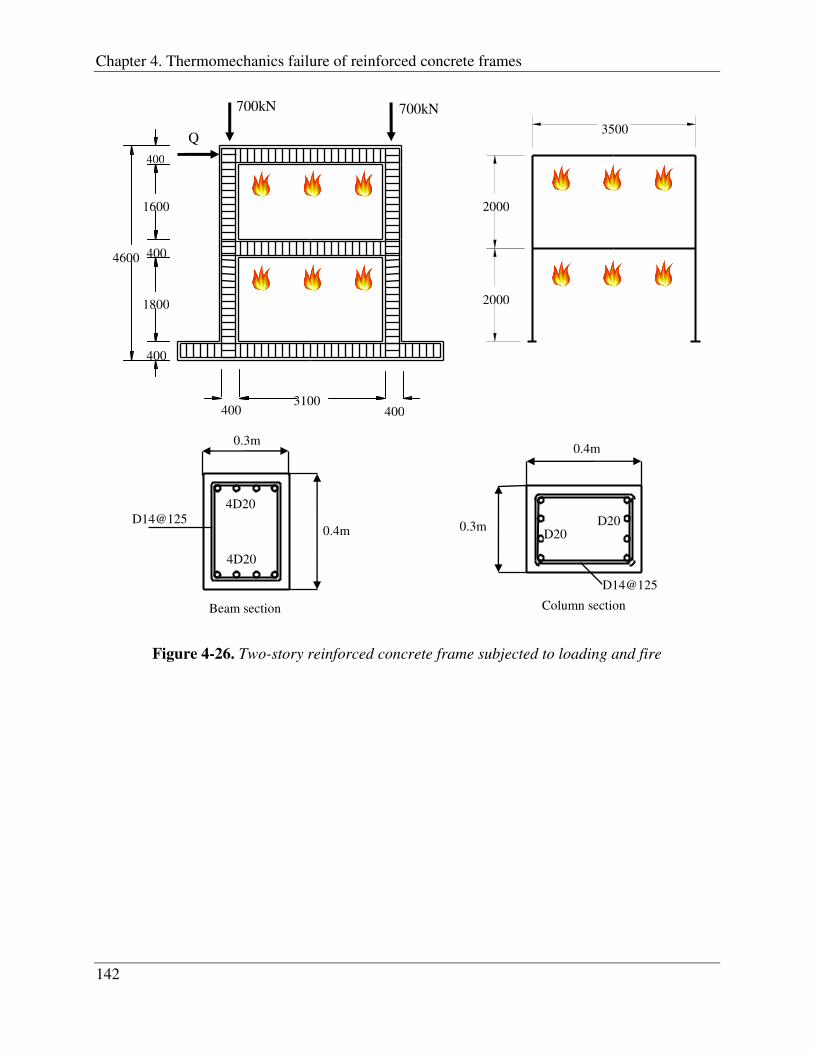
Chapter 4. Thermomechanics failure of reinforced concrete frames
142
Figure 4-26. Two-story reinforced concrete frame subjected to loading and fire
Column section
D20
D14@125
D20 0.3m
0.4m
Beam section
D14@125
4D20
4D20
0.4m
0.3m
400
400
400
1800
400
1600
4600
400 3100
700kN 700kN
Q
2000
2000
3500
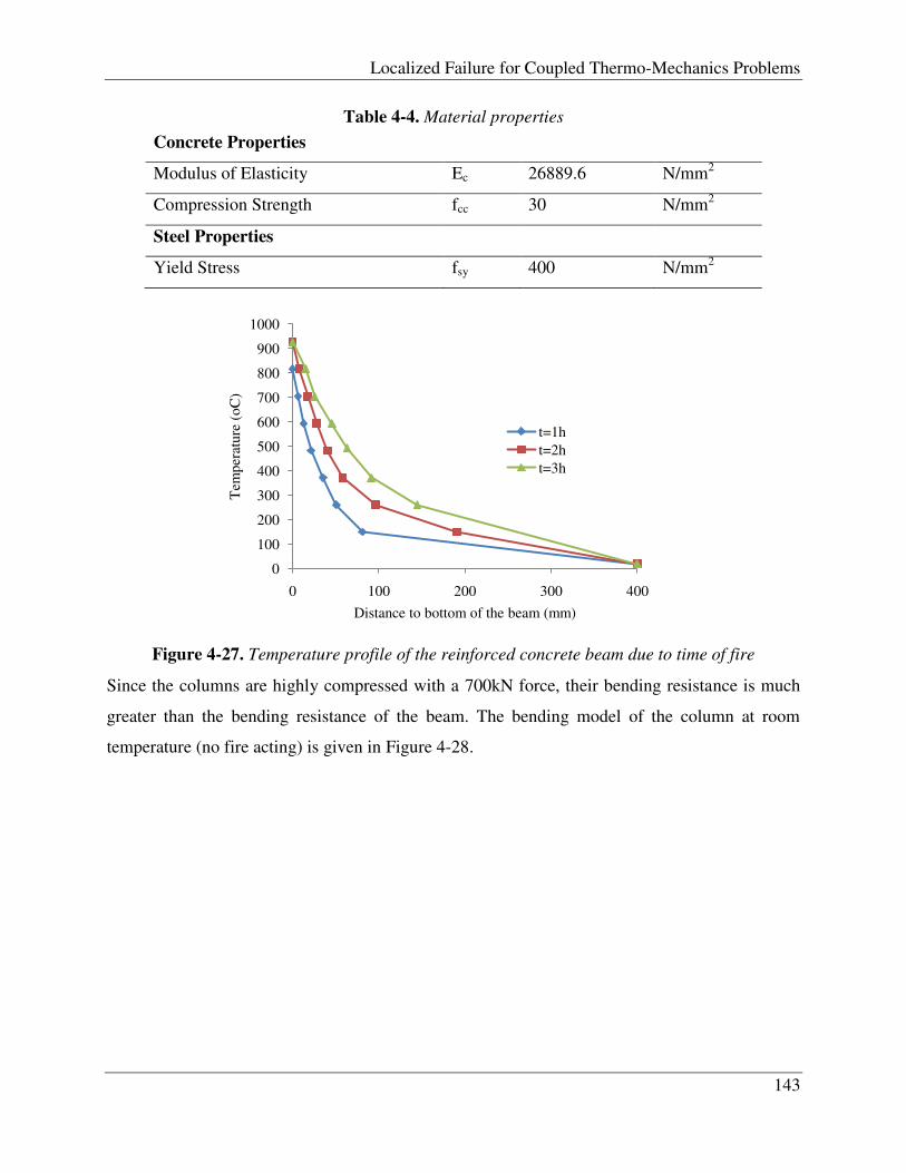
Localized Failure for Coupled Thermo-Mechanics Problems
143
Table 4-4. Material properties
Concrete Properties
Modulus of Elasticity Ec 26889.6 N/mm2
Compression Strength fcc 30 N/mm2
Steel Properties
Yield Stress fsy 400 N/mm2
Figure 4-27. Temperature profile of the reinforced concrete beam due to time of fire
Since the columns are highly compressed with a 700kN force, their bending resistance is much
greater than the bending resistance of the beam. The bending model of the column at room
temperature (no fire acting) is given in Figure 4-28.
0
100
200
300
400
500
600
700
800
900
1000
0 100 200 300 400
Tem
pera
ture
(oC
)
Distance to bottom of the beam (mm)
t=1ht=2ht=3h

Chapter 4. Thermomechanics failure of reinforced concrete frames
144
Figure 4-28. Moment-curvature model for column
The shear model of the column is given in Figure 4-29
Figure 4-29. Shear failure model of the column
Figure 4-30 represents the degradation of moment-curvature curve of the beam after one, two
and three hours exposing to fire.
0
50
100
150
200
250
0 0.02 0.04 0.06 0.08 0.1
Mom
ent (
kN.m
)
Curvature (1/m)
N=700kN
0
50
100
150
200
250
0 0.02 0.04
αŅ(rad)
0
50
100
150
200
250
300
350
400
0 0.00005 0.0001
She
ar F
orce
(kN
)
Shear Strain ( )
0
50
100
150
200
250
300
350
400
0 0.00002 0.00004 0.00006 0.00008
αv (m)

Localized Failure for Coupled Thermo-Mechanics Problems
145
Figure 4-30. Degradation of bending resistance of reinforced concrete beam versus fire
exposure
Figure 4-31 illustrates the reduction of the overall response of the frame due to fire by plotting
the relationship between horizontal force Q with the horizontal displacement of the top beam at
different times: t= 1 hour, t = 2 hours and t = 3 hours.
Figure 4-31.Horizontal force/displacement curve of two-story frame at different instants of fire
0
20
40
60
80
100
120
140
160
180
200
0 0.02 0.04 0.06 0.08 0.1
Mom
ent (
kN.m
)
Curvature (1/m)
t=1h
t=2h
t=3h
0
20
40
60
80
100
120
140
160
180
200
0 0.004
αŅ (rad)
0.05 0.1 0.15 0.2 0.25
0.3 0.35 0.4 0.45 0.5 0
50
100
150
200
250
300
350
Displaceme
Force (kN)
t = 1h
t = 2h
t = 3h
Chapter 4. Thermomechanics failure of reinforced concrete frames
146
We can note, in particular, that the ultimate horizontal load of the reinforced concrete frame
decreases from 308.52kN to 251.46kN and then to 180.01kN after one hour, two hours and three
hours submitted to fire. This is the result of the degradation of the material properties due to high
temperature and also due to the thermal effect on the beam.
4.5 Conclusion
In this chapter we have developed a method to calculate the behavior of reinforced concrete
frame structure subjected to fire, with combined thermal and mechanical loads The main novelty
of the proposed method is its capability of taking into account the thermal loading and the
degradation of material properties due to the temperature in determining the ultimate load of the
reinforced concrete frame. Moreover in the proposed method, we consider not only the bending
failure but also the shear failure of the reinforced concrete structure. This is also a new
contribution in solving the resistance of reinforced concrete frame exposure to fire and thermal
effect. The finite element approach presented for this kind of problem can provide the correct
representation of the localized failure of the reinforced concrete structure. Two most frequent
failure mechanisms are treated separately in order to provide the most robust computational
procedure. The numerical examples we have presented here confirmed a very satisfying results
provided by proposed methodology. The introduced method migh also be used to compute the
remaining resistance of a damaged structure after being subjected to fire loading, which gives the
answer to the question if the damaged consctruction can continue working or not. This proposed
strategy is the first important step towards fully coupled thermomechanical problems to achieve
reliable description of the structural resistance for different thermal load programs and eventual
sudden regime change in the exposure to fire.

Localized Failure for Coupled Thermo-Mechanics Problems
147
5 Conclusions and Perpectives
5.1 Main contributions
In this thesis, we have discussed the general behavior and also the localized failure of steel,
concrete and reinforced concrete structures under extreme thermo-mechanical conditions. The
main contributions concerns both aspects of model theoretical formulation and its numerical
implementation.
In terms of theoretical aspect, new thermo-mechanical models for steel and concrete material
were carried out, providing much better understanding of the interaction between mechanical
response and thermal response of the structure. First, the mechanical dissipation and structural
heating due to inelastic (and/or localized failure) mechanical response will lead to an increase of
the temperature and inversly, the thermal loads and tempertaure gradient will result in a
considerable amount of stress, strain and/or displacement. We have also proved, based on the
local balance equation of energy, that the thermal propagation through a localized failure region
will result in a „jump‟ in the heat flow, or a change in the temperature gradient, in the
localization zone.
In terms of numerical solution, a detailing „adiabatic‟operator split procedure was developed and
applied to solve the present multi-physical problem. Here, the coupled thermo-mechanical
problem is divided into „mechanical‟ process and „thermal‟ process with the „adiabatic‟
constraint condition. The „mechanical‟ process is solved first with the „adiabatic‟ tangent
modulus (taking into account the evolution of temperature due to structural heating) to compute
the mechanical internal variables of the model as well as the mechanical dissipation. Then, the
„thermal‟ process is solved latter based upon a modified form of the classical heat transfer
equation with a corresponding mechanical dissipation acting as an additional heat supply. The
„discontinuity‟ (or a „jump‟) in displacement field and also the „jump‟ in the heat flow at the
localized failure zone are modeled by additional interpolation functions and are determined at the
element level of the operator splitting procedure applying for „mechanical‟ process and „thermal‟
process, respectively. All the problems were solved in the framework of the embedded-
discontinuity finite element method by using the research version of the finite element analysis
program FEAP (see [56], [57]).
Chapter 5. Conclusions and Perpectives
148
The thesis also provided a method to estimate the „ultimate‟ resistance of a reinforced concrete
structure under fire loading. In this method, the structure is considered to be an assembly of
many one-dimensional elements such as : frames, beams and columns, which can be modeled by
Timoshenko beam element. Main novelties of the method are: 1) capability of taking into
account the shear failure (along with the bending failure) into the overal failure of the structure
and 2) capability of taking into account the thermal effect on the total response of the structure.
Both of these two novelties play important roles in analysing the degradation of the reinforced
concrete frame under fire accidents.
5.2 Perpectives
Despite several contributions, one can identify in this thesis a number of deficiencies to be
completed and improved. Chief among them is the need of taking into account the thermo-
mechanical behavior of bonding interface between steel bar and concrete in the total response of
the reinforced concrete structure. How does the bonding interface response under the thermal
loading? How does this response influence the total response of the reinforced concrete
structure? These challenge questions might be studied in the future based on the previous works
of Tran & Sab (see [37]), Davenne et al.(see [63]), Boulkestous et al. (see [64], [26], [65]).
Another development can be expected from this study is to widen the models to accumulate
other behaviors such as the creep and shrinkage of concrete due to age and humidity, as well as
the fatigue and/or buckling behavior of the steel (see [66]). Last but not least, the idea of
extending the proposed theoretical model and the numerical solution to compute the dynamic
response of the structure is also a good direction to go.

Localized Failure for Coupled Thermo-Mechanics Problems
149
6 Bibliography
[1] John L. Gross and Therese P. McAllister,". Structural Fire Response and Probable Collapse
Sequence of the World Trade Center Towers," The United States, 2005.
[2] T. W. Eagar and C. Musso, "Why Did the World Trade Center Collapse? Science,
Engineering, and Speculation," JOM, no. December 2001, 2001.
[3] T. Foecke, W.E.Luecke, J.D. McColskey, C.N. McCowan, T.A. Siewert, F.W. Gayle S.W.
Banovic, "The Role of Metallurgy in the NIST Investigation of the World Trade Center
Towers Collapse," JOM, no. December 2007, December 2007.
[4] Society of Fire Protection Engineers, "Guidelines for Designing Fire Safety in Very Tall
Buildings," 2012.
[5] A. J. C. B. Saint-Venant, "Memoire sur la Torsion des Prismes," Mémoires présentés par
divers savants, vol. 14, pp. 233-560, 1855.
[6] EN 1993-1-2, "Eurocode 3. Design of steel structures. Part 1.2 : General rules. Structure fire
design," 2005.
[7] EN-1992-1-2, Eurocode 2: Design of Concrete Structure - Part 1-2: General rules-
Structural Fire Design.: Eurocode, 2004.
[8] ACI-216, Standard Method for Determining Fire Resistance of Concrete and Mansonry
Construction Assemblies.: American Concrete Institute, 1997.
[9] ACI-318, Building Code Requirements for Structural Concrete and Commentary.:
American Concrete Institute , 2008.
[10] ASCE-1992, Structural Fire Protection. New York: ASCE Manual and Reports on
Engineering Practice, 1992.
[11] ASTM-E119, Standard Test Methods for Fire Tests of Building Construction and Material.:
American Society for Testing and Materials, 2000.
[12] AASHTO-LRFD-2012, "AASHTO LRFD Bridge Design Specifications," 2012, 2011.
150
[13] V.K.P Kodur and M. Dwaikat, "A Numerical Model for Predicting the Fire Resistance of
Reinforced Concrete Beams.," Cement & Concrete Composites, pp. 431-443, 2008.
[14] M. Dwaikat and V.K.P Kodur, "A Numerical Approach for Modeling the Fire Induced
Restraint Effects in Reinforced Concrete Beams.," Fire Safety Journal. Volume 43, pp. 291-
307, 2008.
[15] J.H Hsu and C.S. Lin, "Residual Bearing Capabilities of Fire-Exposed Reinforced Concrete
Beams.," International Journal of Applied Science and Engineering. Volume 4, pp. 151-163,
2006.
[16] D. Di Capua and A.R Mari, "Nonlinear Analysis of Reinforced Concrete Cross-Section
Exposed to Fire," Fire Safety Journal, vol. 103, no. 4, pp. 139-149, 2007.
[17] A. Ibrahimbegovic, Nonlinear Solid Mechanics: Theoretical Formulation and Finite
Element Solution Methods.: Springer, 2009.
[18] A. Ibrahimbegovic and E.L Wilson, "A Modified Method of Incompatible Modes.,"
Communications in Applied Mechanics Methods, pp. 187-194, 1991.
[19] B.H. Pham, "Stress-Resultant Models for Optimal Design of Reinforced Concrete Frames.,"
Cachan. France, 2009.
[20] B.H. Pham, L. Davenne, D. Brancherie, and A. Ibrahimbegovic, "Stress Resultant Model for
Ultimate Load Design of Reinforced Concrete Frames: Combined Axial Force and Bending
Moment.," Computers and Concrete, pp. 303-315, 2010.
[21] N.N Bui, V.M Ngo, D. Brancherie, and A. Ibrahimbegovic, "Enriched Timoshenko beam
finite element for modelling bending and shear failure of reinforced concrete frames,"
Computer and Structures, vol. submitted.
[22] A. Ibrahimbegovic and S. Melnyk, "Embedded discontinuity finite element method for
modeling of localized failure in heterogeneous materials with structured mesh: an
alternative to extended finite element method," Computational Mechanics, vol. 40, pp. 149-
155, 2007.
Localized Failure for Coupled Thermo-Mechanics Problems
151
[23] A. Ibrahimbegovic and D. Brancherie, "Combined hardening and softening constitutive
model of plasticity: precursor to shear slip line failure," Computational Mechanics, pp. 88-
100, 2003.
[24] D. Brancherie, "εodeles continus et “discrets” pour les problemes de localisation et de
rupture fragile et/ou ductile," Cachan, 2003.
[25] D. Brancherie and A. Ibrahimbegovic, "Novel anisotropic continuum-discrete damage
model capable of representing localized failure of massive structures. Part I: theoretical
formulation and numerical," International Journal for Computer-Aided Engineering and
Software, vol. 26, pp. 100-127, 2009.
[26] A. Ibrahimbegovic, A. Boulkertous, L. Davenne, and D. Brancherie, "Modeling of
Reinforced Concrete Structures Providing Crack-Spacing based on X-FEM, ED-FEM and
novel operator split solution procedure," International Journal for Numerical Methods in
Engineering, vol. 83, pp. 452-481, 2010.
[27] M. Ortiz, Y. Leroy, and A. Needleman, "A finite element method for localized failure
analysis," Computer Methods in Applied Mechanics and Engineering, vol. 61, no. 2, pp.
189-214, March 1987.
[28] J. Oliver, F. Armero J. C. Simo, "An analysis of strong discontinuities induced by strain-
softening in rate-independent inelastic solids," Computational Mechanics, vol. 12, no. 5, pp.
277-296, 1993.
[29] F. Armero, "Localized anisotropic damage of brittle materials," in 5th, Computational
plasticity: fundamentals and applications, 1997, pp. 635-640.
[30] F. Armero and K. Garikipati, "Recent advances in the analysis and numerical simulation of
strain localization in inelastic solids," in 4th Computational Plasticity: Fundamentals and
Applications., Barcelona, 1995, pp. 547–561.
[31] F. Armero, "Large-scale modeling of localized dissipative mechanisms in a local
continuum: applications to the numerical simulation of strain localization in rate-dependent
inelastic solids," Mechanics of Cohesive-frictional Materials, vol. 4, no. 2, pp. 101-131,

152
March 1999.
[32] J. Oliver, "Modelling strong discontinuities in solid mechanics via strain softening
constitutive equations. Part I& Part II," International Journal for Numerical Methods in
Engineering, vol. 39, pp. 3575-3623, 1996.
[33] F. Armero and J.C. Simo, "A priori stability estimates and unconditionally stable product
formula algorithms for nonlinear coupled thermoplasticity," International Journal of
Plasticity, vol. 9, no. 6, 1993.
[34] A. Ibrahimbegovic and L. Chorfi, "Covariant principal axis formulation of associated
coupled thermoplasticity at finite strains and its numerical implementation," International
Journal of Solids and Structures, vol. 39, pp. 499-528, 2002.
[35] A. Ibrahimbegovic, L.Chorfi, and F. Gharzeddine, "Thermomechanical Coupling at Finite
Elastic Strain: Covariant Formulation and Numerical Implementation," Communications in
Numerical Methods in Engineering, vol. 17, pp. 275-289, 2001.
[36] G. Baker and R. de Borst, "An anisotropic thermomechanical damage model for concrete at
transient elevated temperatures," Philosophical transactions. Mathematical physical and
engineering, vol. 363, no. 1836, pp. 2603-2628, 2005.
[37] ζ.C Tran, "Développement d‟un modèle d‟interface béton-acier à haute température.
Modélisation des structures en béton exposées au feu.," École des Ponts ParisTech,
Université Paris-Est, Ph.D Thesis 2011.
[38] K. Runession, P. Steinmann, and R. Larsson, "On localization in thermo-elastoplastic solids
subjected to adiabatic conditions," European Journal of Mechanics- A/Solids, vol. 18, pp.
557-579, 1999.
[39] F. Armero and J. Park, "An analysis of strain localisation in a shear layer under thermally
coupled dynamic conditions. Part 2: Localized thermoplastic model," International Journal
for Numerical Methods in Engineering, vol. 56, no. 14: Computational Failure Mechanics,
pp. 2101-2133, April 2003.
[40] K. William, I. Rhee, and B. Shing, "Interface Damage Model for Thermomechanical

Localized Failure for Coupled Thermo-Mechanics Problems
153
Degradation of Heterogeneous Materials," Computer Methods in Applied Mechanics and
Engineering, vol. 1993, no. 30-32: Computational Failure Mechanics, pp. 3327-3350, July
2004.
[41] F.J Vecchio and M.P. Collins, "Predicting the Response of Reinforced Concrete Beams
Subjected to Shear Using Compression Field Theory," ACI Structural Journal, pp. 258-268,
1988.
[42] J.C. Simo and C. Miehe, "Associative coupled thermoplasticity at finite strains:
Formulation, numerical analysis and implementation," Computer Methods in Applied
Mechanis and Engineering, vol. 98, no. 1, pp. 41-104, 1992.
[43] J.B. Colliat, A. Ibrahimbegovic, and L. Davenne, "Modeling thermomechanical behaviour
of cellular structure made of brittle material," 2003.
[44] V.M. Ngo, A. Ibrahimbegovic, and D. Brancherie, "Continuum damage model for thermo-
mechanical coupling in quasi-brittle materials," Engineering Structure, vol. 50, pp. 170-178,
2013.
[45] D. Gawin, C.E. Majorana, F. Pesavento, and B.A. Schrefle, "A fully compled multiphase FE
model of hygro-thermo-mechanical behavior of concrete at high temperature," in
Computational Mechanics: New Trends and Application, Barcelona, 1998.
[46] C. Kassiotis, J.B. Colliat, and A. Ibrahimbegovic, "Multiscale in time and stability analysis
of operator split solution procedures applied to thermomechanical problems," International
Journal for Computer-Aided Engineering and Software, vol. 26, 2009.
[47] M. Gross and P. Betsch, "Galerkin-based energy-momentum consistent time-stepping
algorithms for classical nonlinear thermo-elastodynamics," vol. 82, no. 4, pp. 718-770,
December 2001.
[48] T. Belytschko and T. Black, "Elastic crack growth in finite elements with minimal
remeshing," International Journal for Numerical Methods in Engineering, vol. 45, pp. 601-
620, 1999.
[49] A. Ibrahimbegovic and D. Brancherie, "Combined hardening and softening constitutive

154
model of plasticity: precursor to shear slip line failure," Computational Mechanics, vol. 31,
pp. 88-100, 2003.
[50] C. Kassiotis, J.B. Colliat, A. Ibrahimbegovic, and H. Matthies, "Multiscale in time and
stability analysis of operator split solution procedure," International Journal of Engineering
Computations, vol. 26, pp. 205-223, 2009.
[51] M. Ortiz and E.P. Popov, "Accuracy and stability of integration algorithms for elastoplastic
constitutive relations," International Journal for Numerical Methods in Engineering, vol.
21, no. 9, pp. 1561-1576, 1985.
[52] F. Armero and C. Linder, "New finite elements with embedded strong discontinuities in the
finite deformation range," Computer Methods in Applied Mechanics and Engineering, pp.
3138-3170, 2008.
[53] V.M. Ngo, A. Ibrahimbegovic, and D. Brancherie, "Model for localized failure with thermo-
plastic coupling. Theoretical formulation and ED-FEM implementation," Computers and
Structures, vol. 127, pp. 2-18, 2013.
[54] C. Farhat, K.C. Park, and Y. Dubois-Pelerin, "An unconditionally stable staggered
algorithm for transient finite element analysis of coupled thermoelastic problems," vol. 85,
pp. 349-365, 1991.
[55] Claus V. Nielsen, Chris J. Pearce, and Nenad Bicanic, "Improved phonomenological
modelling of transient thermal strains for concrete at high temperatures," Computers and
Concrete. Volume 1, pp. 189-209, 2004.
[56] R. Taylor, "FEAP - A Finite Element Analysis Program. Version 7.5 User Manual," 2004.
[57] R. Taylor, "FEAP - A Finite Element Analysis Program. Version 7.5. Programmer Manual,"
2004.
[58] F.J Vecchio and Emara, "Shear Deformation in Reinforced Concrete Frames," ACI
Structural Journal, pp. 46-56, 1992.
[59] D. Bentz, F.J. Vecchio, and M.P. Collins, "Simplifed Modified Compression Field Theory

Localized Failure for Coupled Thermo-Mechanics Problems
155
for Calculating Shear Strength of Reinforced Concrete Elements," ACI Structural Journal,
no. 103-S65, pp. 614-624, 2006.
[60] T.T.H Le, "Etude multi-échelles du comportement Thermo-Hydro-Mécanique des
matériaux cimentaires. Approche morphologique pour la prise en compte de la
mésostructure," France, 2011.
[61] F.J. Vecchio and M.P. Collins, "Predicting the Response of Reinforced Concrete Beams
Subjected to Shear Using Compression Field Theory," ACI Structural Journal., pp. 258-
268, 1988.
[62] A. Ibrahimbegovic and F. Frey, "Stress Resultant Finite Element Analysis of Reinforced
Concrete Plates," Engineering Computations, vol. 10, no. 1, pp. 15-30, 1993.
[63] L. Davenne and A. Ibrahimbegovic A. Boulkestous, "Influence of the steel-concrete bond-
slip on the behavior of RC structures under severe conditions," in CONSEC10, 2010.
[64] 17. A. Ibrahimbegovic, A. Boulkertous, M. Muhasilovic L. Davenne, J. Duhovnik, and A.
Pokrklic, "Fire Induced Damage in Structures and Infrastructure: Analysis, Testing and
Modeling," Damage Assesment and Reconstruction after War or Natural Disaster, pp. 321-
342, 2009.
[65] A. Ibrahimbegovic, A. Boulkertous, L. Davenne, and M., Pokrklic, A. Muhasilovic, "On
modeling of fire resistance tests of concrete and reinforced-concrete structures.," Computers
& Concrete, vol. 7, pp. 285-302, 2010.
[66] J. Besson, G. Cailletaud, JL. Chaboche, and S. Forest, Mécanique non linéaire des
matériaux, Hermès, Ed.: Lavoisier, 2001.
[67] H.F.B Xavier, "Analysis of Reinforced Concrete Frames Exposed to Fire: Based on
Advanced Calculation Methods," Porto, 2009.
[68] A. Ibrahimbegovic, J.B. Colliat, and L. Davenne, "Thermomechanical coupling in folded
plates and non-smooth shells," Computer Methods in Applied Mechanics and Engineering,
vol. 194, pp. 2686-2707, 2005.

156
[69] I. Romero, "Thermodynamically consistent time-stepping algorithms for non-linear
thermomechanical systems," International Journal for Numerical Methods in Engineering,
pp. 706-732, 2009.
[70] A. Kucerova, D. Brancherie, A. Ibrahimbegovic, J. Zeman, and Z. Bittnar, "Novel
anisotropic continuum-discrete damage model capable of representing localized failure of
massive structures. Part II: identification from tests under heterogeneous stress field,"
Engineering Computations: International Journal for Computer-Aided Engineering and
Software, vol. 26, pp. 128-144, 2009.
[71] N. Mathieu, K. Sab, and S.A. Zaïmi, "An enhanced homogenization approach for masonry
structures with compressible joints. Application to hearth thermomechanical
computations.," International Journal for Numerical and Analytical Methods in
Geomechanics, vol. 36, no. 9, pp. 1102-1124, June 2012.