the role of production risk in sustainable land ... sustainable land- management technology adoption...

Environment for Development

Discussion Paper Series Apr i l 2008 EfD DP 08-15

The Role of Production Risk in Sustainable Land- Management Technology Adoption in the Ethiopian Highlands

Mena le Kass ie , Mahmud Yesuf , and Gunnar Köh l in

Environment for Development

The Environment for Development (EfD) initiative is an environmental economics program focused on international research collaboration, policy advice, and academic training. It supports centers in Central America, China, Ethiopia, Kenya, South Africa, and Tanzania, in partnership with the Environmental Economics Unit at the University of Gothenburg in Sweden and Resources for the Future in Washington, DC. Financial support for the program is provided by the Swedish International Development Cooperation Agency (Sida). Read more about the program at www.efdinitiative.org or contact [email protected].

Central America Environment for Development Program for Central America Centro Agronómico Tropical de Investigacíon y Ensenanza (CATIE) Email: [email protected]

China Environmental Economics Program in China (EEPC) Peking University Email: [email protected]

Ethiopia Environmental Economics Policy Forum for Ethiopia (EEPFE) Ethiopian Development Research Institute (EDRI/AAU) Email: [email protected]

Kenya Environment for Development Kenya Kenya Institute for Public Policy Research and Analysis (KIPPRA) Nairobi University Email: [email protected]

South Africa Environmental Policy Research Unit (EPRU) University of Cape Town Email: [email protected]

Tanzania Environment for Development Tanzania University of Dar es Salaam Email: [email protected]

© 2008 Environment for Development. All rights reserved. No portion of this paper may be reproduced without permission of the authors.

Discussion papers are research materials circulated by their authors for purposes of information and discussion. They have not necessarily undergone formal peer review.

The Role of Production Risk in Sustainable Land-Management Technology Adoption in the Ethiopian Highlands

Menale Kassie, Mahmud Yesuf, and Gunnar Köhlin

Abstract This paper provides empirical evidence of production risk impact on sustainable land- management

technology adoption, using two years of cross-sectional plot-level data collected in the Ethiopian highlands. We used a moment-based approach, which allowed a flexible representation of the production risk (Antle 1983, 1987). Mundlak’s approach was used to capture the unobserved heterogeneity along with other regressors in the estimation of fertilizer and conservation adoption. The empirical results revealed that impact of production risk varied by technology type. Production risks (variance and crop failure as measured by second and third central moments, respectively) had significant impact on fertilizer adoption and extent of adoption. However, this impact was not observed in adoption of conservation technology. On the other hand, expected return (as measured by the first central moment) had a positive significant impact on both fertilizer (adoption and intensity) and conservation adoption. Economic instruments that hedge against risk exposure, including downside risk and increase productivity, are important to promote adoption of improved technology and reduce poverty in Ethiopia.

Key Words: Production risk, sustainable land management technology adoption, moment based estimation, Ethiopia

JEL Classification Numbers: D81, D13, C33, Q24, O33

Contents

1. Introduction......................................................................................................................... 1

2. Literature Review .............................................................................................................. 3

3. Conceptual Model .............................................................................................................. 4

4. Empirical Methodology..................................................................................................... 6

4.1. Econometric Estimation Procedures and Techniques................................................. 6

4.2. Econometric Estimation Challenges and Remedies ................................................. 11

5. Data Sources and Types .................................................................................................. 13

6. Results and Discussion..................................................................................................... 17

7. Summary and Conclusion ............................................................................................... 20

References.............................................................................................................................. 21

Environment for Development Kassie, Yesuf, and Köhlin

1

The Role of Production Risk in Sustainable Land-Management Technology Adoption in the Ethiopian Highlands

Menale Kassie, Mahmud Yesuf, and Gunnar Köhlin∗

1. Introduction

Increased adoption of improved technologies remains the key to achieving food security in Ethiopia, where agriculture is mainly characterized by little use of external inputs, low productivity, high nutrient depletion, and soil erosion that limit farmers’ ability to increase agricultural production and reduce poverty and food insecurity. Extension and credit services are some of the initiatives that the government of Ethiopia has implemented to promote the adoption of improved technology through its development strategy, known as Agricultural Development-Led Industrialization (ADLI). Non-government organizations (NGOs) and donors have also implemented various kinds of food-for-work projects to disseminate soil conserving technologies. Despite such concerted efforts by the government and NGOs, the adoption rate of improved technology remains low, and there is even some evidence that conservation structures, once constructed, are partially or fully removed by the farmers. In some cases, pilot demonstration projects cannot be replicated on smallholder farms (Shiferaw and Holden 2001).

Production risks play an important role in agricultural production decisions—particularly in input choices—and contribute toward worsening social welfare in the absence of mechanisms that serve to minimize its downside effects (Antle 1983, 1987; Dercon 2004). For risk aversion, an increase in variance tends to make the decision maker worse off. A fair amount of empirical evidence suggests that most decision makers exhibit decreasing absolute risk aversion (e.g., Binswanger 1981; Chavas and Holt 1996; Chavas 2004), implying downside risk aversion (Menezes et al. 1980; Antle 1987). Therefore, in addition to variance of return, downside risk (e.g., extreme drought and rainfall leading to crop failure) may have an impact on improved technologies adoption. (See section 3 for more on variance and downside risk.)

∗ Menale Kassie, Environmental Economics Policy Forum for Ethiopia, Ethiopian Development Research Institute, Blue Building/Addis Ababa near National Stadium, P.O. Box 2479, Addis Ababa, Ethiopia, (email) menalekassie @yahoo.com, (tel) + 251 11 5 506066, (fax) +251 115 505588; Mahmud Yesuf, Environmental Economics Policy Forum for Ethiopia, Ethiopian Development Research Institute, Blue Building/Addis Ababa Stadium, P.O. Box 2479, Addis Ababa, Ethiopia, (email) [email protected], (tel) + 251 11 5 506066, (fax) +251 115 505588; and Gunnar Köhlin, Department of Economics, University of Gothenburg, P.O. Box 640, 405 30 Gothenburg, Sweden, (email) [email protected], (tel) + 46 31 786 4426, (fax) +46 31 7861043.


2

Although a number of studies in the adoption literature1 have reported on the determinants of adoption, the link between production risk and technology adoption has not been adequately addressed. A notable exception is the work of Koundouri et al. (2006), which assessed the impact of production risk on irrigation technology adoption, using moments of profit from cross-sectional data collected from 265 farm households in Crete, Greece. However, this study suffered from econometric problems. The unobserved heterogeneity that may influence technology adoption and production decisions and risk management strategies was not controlled for.

The objective of this paper is to provide empirical evidence of the effect of risk exposure, including the downside risk of chemical fertilizer and soil and water conservation adoption (hereafter technology adoption). Following Antle (1983, 1987), Antle and Goodger (1984), and Koundouri et al. (2006), we used a flexible representation of uncertainty by using estimated moments of value of crop production (here after return) 2 as determinants of technology adoption. The panel nature of the data collected in the Ethiopian highlands allowed us to control for unobservable characteristics that otherwise would bias (selection and endogeneity biases) the results and possibly lead to wrong conclusions.

The empirical analysis showed that risk plays a significant role in technology adoption. The first moment, which approximated expected return, was highly significant in the soil and water conservation technology (hereafter conservation technology) adoption random effects model. The higher the expected return, the greater the probability that farmers would decide to adopt conservation technology, as they expected to be able to afford the adoption of new soil conservation measures. The second and third moments, which approximated variance and skewness of return, were not statistically significant in the conservation random-effects probit model, implying that long-term investments were not affected by production risk. On the other hand, the probability of fertilizer adoption and its intensity was significantly affected by the first, second, and third moments, which approximated expected return and variance and skewness of return, respectively. The adoption and intensity decreased for farmers who experienced higher variance of return and downside risk exposure (skewness), and increased for farmers who experienced higher expected return. The empirical finding could provide guidance to decision

1 We refer to Feder and Umali (1990) and the reference therein for a detailed review of the determinants of technology adoption. 2 It is obtained by multiplying the physical quantity by the average local price of each crop.


3

makers and help them design economic instruments that can hedge against variability of return (as measured by variance) and crop failure and increase expected return to promote sustainable land management technologies.

The rest of the paper is organized as follows: section 2 presents a brief review of previous empirical works. In section 3, we discuss a conceptual framework used to analyze the farmer’s decision in the presence of production risk. Following a discussion on econometric methodology in section 4, a description of the dataset is presented in section 5. The empirical results are presented in section 6. Finally, section 7 summarizes the main findings and concludes the paper.

2. Literature Review

Modern inputs, such as fertilizer and adoption of soil and water conservation technologies are important determinants of agricultural productivity, and continuing high agricultural productivity is an important strategy for escaping poverty, especially in agriculture-based countries in sub-Saharan Africa (Christiaensen and Demery 2007; Morris et al. 2007). However, adoptions of both of these technologies are limited in many of these countries. In the theoretical literature, risk exposure and risk avoidance are often associated with low adoption rates, low income, and continuing poverty traps in many low-income countries (Rosenzweig and Binswanger 1993).

When investment decisions are constrained by either ex-ante resource constraints—such as credit—or lack of ex-post coping mechanisms—such as both formal and informal insurance—risk will cause farmers to be less willing to undertake activities and investments that have not only higher expected outcomes but also risks of failure or downside risk (Just and Pope 1979; Rosenzweig and Binswanger 1993). This leads to risk-induced poverty traps, whereby those who can self-finance their investment activities or insure their consumption against income shocks can take advantage of the most profitable opportunities and possibly grow out of poverty. Others, unfortunately, are stuck with low-return, low-risk activities which trap them in poverty (Rosenzweig and Binswanger 1993; Moseley and Verschoor (2004); Dercon and Christiaensen 2007). Thus, understanding risk exposure in the face of incomplete credit or insurance may be key to understanding limited adoption of yield-enhancing technologies, such as fertilizer use or soil conservation technologies. In such an environment, there would be substantial synergies in complementing interventions that foster access to credit with interventions that help households cope with shocks (e.g., insurance) —a critical insight for the design of effective poverty-reducing strategies.


4

In the empirical literature, using either econometric or bio-economic models, a host of demand- and supply-side factors have been invoked to explain the limited adoption of fertilizer and/or soil and water conservation technologies in sub-Saharan African countries in general and in Ethiopia specifically. Among others, these include tenure insecurity (Deininger et al. 2003; Benin and Pender 2001; Holden and Yohannes 2002; Gebremedhin and Swinton 2003; Alemu 1999), household endowments of physical and human capital (Asfaw and Admassie 2004; Pender and Fafchamps 2005; Ersado et al. 2003), agricultural extension, credit and market access (Abrar et al. 2004; Mulat et al. 1998; Holden and Shiferaw 2004), limited off-farm opportunities (Pender and Gebremedhin 2004; Pender et al. 2003), limited profitability (Croppenstedt et al. 2003; Dadi et al. 2004; World Bank 2006), and population pressure (Grepperud 1996). A recent study has also highlighted the importance of households’ limited ex-post consumption-coping capacity to low adoption rates of fertilizers in Ethiopia (Dercon and Christiaenson 2007). There is also some mixed evidence of the impact of inherent risk preferences on fertilizer adoptions in Ethiopia (Hagos 2003; Yesuf 2004) and time preference on soil and water conservation technology adoptions (Shiferaw and Holden 1998; and Yesuf 2004).

Despite their critical role in designing appropriate policies and strategies, studies on the impact of risk exposure on technology adoption are almost non-existent.

3. Conceptual Model

Following Koundouri et al. (2006), this section describes the theoretical framework we used to explain farm households’ investment and production decisions. Since farm households in developing countries that undertake agricultural production face production uncertainty and multifaceted market imperfection, we used an expected utility maximization framework to represent investment and production decisions made under uncertainty. The production risk is represented by a random variable, hpε , whose distribution (.)G is exogenous to the farmer’s

action. We assumed prices—both input ( )r and output ( )p —are non-random (i.e., farmers are assumed to be price takers in both markets). Chemical fertilizer )( f

hpx and conservation effort

)( chpx applied on p by household h are assumed to be an essential input in the production

process. Assuming risk-averse farmers, the farm household’s problem is to maximize the expected utility of gross income as defined below:

[ ] [ ] }{[ ] )(,,,,((max)((max εψεπ dGxrxrxrxxxpfUEUEE ohpo

chpc

fhpfh

ohp

chp

fhphpxx ∫ −−−= (1)

where E is the expectation operator, π is the per-period return from farming, f is the well-behaved (continuously and twice differentiable) production function, and (.)U is the von


5

Neumann-Morgenstern utility function. ohpx is the vector of other plot and plot invariant

observed variables, including plot size, other plot level inputs, farmer characteristics and endowments, and location (district) dummy variables; and hψ is the unobserved household

heterogeneity that captures unreported household characteristics, such as farm management ability, average land fertility, risk management strategies, risk preferences, time preferences, etc., that affect input use and productivity.

Given that and p r are non-random, the first order condition (FOC) for fertilizer and

variable is rewritten as follows (for ease of notation, we dropped the subscripts):

⎥⎥⎦

⎤

⎢⎢⎣

⎡

∂

∂= '' ),,,,(

)( Ux

xxxfpEUrE f

hp

hohp

chp

fhphp

f

ψε (1a)

)()),,,,(;cov(),,,,(

'

'

UExxxxfU

xxxxf

Epr f

hphohp

fhp

fhphp

fhp

hohp

chp

fhphpf ∂∂

+⎥⎥⎦

⎤

⎢⎢⎣

⎡

∂

∂=

ψεψε (1b)

where 'U is the change in the utility of income as a result of change in income ( )U ππ

∂⎡ ⎤⎢ ⎥∂⎣ ⎦

. A

similar procedure can be followed to derive the FOCs of conservation and other variables. For risk-neutral farmers, the first term in the right-hand side of equation (1b) will disappear and adoption of technology will depend on the classical marginal conditions. For risk-averse farmers, this term is different from zero. In this case, whether farmers adopt technology will be governed by production risk in addition to adoption costs and other factors. Farm-specific attributes, such as plot quality and slope, may influence adoption decisions by influencing technology performance or adoption costs.

When market imperfections are important, inclusion of household characteristics and resource endowments to explain investment and production decision is important (Pender and Kerr 1998; Holden et al. 2001), in addition to other determinants of investment and production decisions. For instance, imperfection in labor markets forces households to equate labor demands with family labor supply. Thus, larger families—with a greater labor supply—are more likely to adopt labor-intensive technologies. The same can be said about credit or capital market imperfections. Households with more savings or productive assets will be able to invest if the technologies are capital intensive. Pender and Kerr (1998) found that imperfections in labor markets led to differences in soil and water conservation investments among farmers in India (Aurepalle village), where investment was greater among households that had more adult males and fewer adult females, and farmed less land.


6

A farmer only adopts improved technology if the expected utility with adoption 1( )E U π⎡ ⎤⎣ ⎦ is greater than the expected utility without adoption 0( )E U π⎡ ⎤⎣ ⎦ . That is:

1 0( ) ( ) 0E U E Uπ π⎡ ⎤ ⎡ ⎤− >⎣ ⎦ ⎣ ⎦ (2)

4. Empirical Methodology

This section outlines the econometrics methods and models used to examine the determinants of technology adoption and intensity and value of production. We compared one-step versus two-step econometric estimation of fertilizer use.

4.1. Econometric Estimation Procedures and Techniques

Risk-averse decision makers have an incentive to reduce their risk exposure. Farm households in low-income countries are typically risk averse (Dercon 2004). Their welfare suffers (welfare loss) when they experience a fluctuation or variability (e.g., as measured by variance) in their production or consumption pattern. However, variability may not completely capture the extent of risk exposure. The variance also does not distinguish between an unexpected bad event compared to an unexpected good one (Di Flaco and Chavas 2006). As a result, we went beyond variance and introduced skewness into risk analysis. The skewness of crop production can capture the probability of crop failure, where negative skewness reflects a greater exposure to downside risk (ibid.).

The econometric estimation of production-risk impact on technology adoption follows two steps. First, we computed the first three sample moments of return distribution of each plot, namely the mean, variance, and skewness coefficients.3 In the second stage, the estimated moments along with other explanatory variables were included in the adoption models. The empirical estimation of the analysis of these moments was conducted as follows in equation (3). (See Kim and Chavas 2003 and Koundouri et al. 2006 for details of the estimation procedure.)

In the first step, value of crop production per plot was regressed using observed and unobserved plot-level variables (including fertilizer and soil conservation variables) and

3 Usually, higher moments have less influence on the dependent variable (Antle 1987). Therefore, our analysis concentrated on the first three moments (mean, variance, and skeweness).


7

household- and village-level variables to get estimates of the mean effect. The model has the following general functional form:

hphohp

chp

fhphp xxxfy εβψ += ),,,,( 11 (3)

where hpy is value of production obtained and used by household h on plot ;p hpε is the

random variable which summarizes the plot-specific component, other than the ones reported in the survey—such as unobserved variation in plot quality and plot-specific production shocks (e.g., plot-level variations in rainfall, hail, frost, floods, weeds, pests, and disease infestations); and 1β is a vector of parameters to be estimate.

Then, the thj central moment of value of crop production about its mean is defined as:

[ ]{ },(.) 1(.)j

j Ye με −= for ,,...,2 mj = (4)

where μ denotes the mean value of crop production or first moment of value of crop production per plot. The estimated errors from the mean regression )ˆ,,,,( 11 βψε h

ohp

chp

fhphp xxxf− are

estimates of the first moment of value of crop production distribution. The estimated errors hpε

are then squared and regressed on the same set of explanatory variables as in equation (5):

hphohp

chp

fhphp xxxf υβψε += )ˆ,,,,( 22

2 . (5)

The least square estimates of 2β̂ are consistent and asymptotically normal (Antle 1983; Antle and Goodger 1984). The predicted values of 2ˆhpε are consistent estimates of the second

central moment (variance value of crop production) of the value of crop-production distribution. Using the same procedure, we can estimate skewness (the estimated errors raised to the power of three). Examples of previous studies using the above approach include (Antle 1983; Antle and Goodger 1984; Kim and Chavas 2003; Koundouri et al. 2006).

Plot-level censoring of input use in the case of fertilizer required a different econometric approach than for the mean function and other moments. One basic issue was whether the decision to use fertilizer or not on a plot was driven by variables and processes other than the related decision on how much fertilizer to use. There may be no good a priori knowledge that tells which model is the correct one. A cautious approach was chosen to test alternative models and combinations of models.

Where a dependent variable contains both zero and non-zero values, a Tobit model and variants of Tobit models, such as Cragg and lognormal (hereafter Wooldridge model) models, may handle this problem. Nested (log-likelihood ratio test) and non-nested (Voung test) model


8

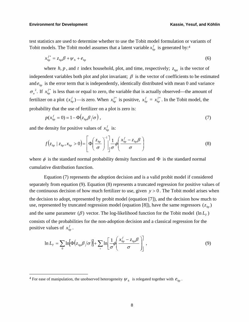
test statistics are used to determine whether to use the Tobit model formulation or variants of Tobit models. The Tobit model assumes that a latent variable f

hpx is generated by:4

hphhpf

hp ezx ++= ψβ* (6)

where ,h p , and t index household, plot, and time, respectively; hptz is the vector of

independent variables both plot and plot invariant; β is the vector of coefficients to be estimated and hpe is the error term that is independently, identically distributed with mean 0 and variance

2.uσ If *fhpx is less than or equal to zero, the variable that is actually observed—the amount of

fertilizer on a plot )( fhpx —is zero. When *f

hpx is positive, fhpx = *f

hpx . In the Tobit model, the

probability that the use of fertilizer on a plot is zero is:

( )σβhpf

hp zxp Φ−== 1)0( , (7)

and the density for positive values of fhpx is:

( ) ⎟⎟⎠

⎞⎜⎜⎝

⎛ −

⎥⎥⎦

⎤

⎢⎢⎣

⎡⎟⎟⎠

⎞⎜⎜⎝

⎛Φ=>

−

σβ

φσσ

hpf

hphphphphp

zxzxzzf 10,|

1

(8)

where φ is the standard normal probability density function and Φ is the standard normal

cumulative distribution function.

Equation (7) represents the adoption decision and is a valid probit model if considered separately from equation (9). Equation (8) represents a truncated regression for positive values of the continuous decision of how much fertilizer to use, given 0>y . The Tobit model arises when

the decision to adopt, represented by probit model (equation [7]), and the decision how much to use, represented by truncated regression model (equation [8]), have the same regressors )( hpz

and the same parameter ( )β vector. The log-likelihood function for the Tobit model )(ln TL

consists of the probabilities for the non-adoption decision and a classical regression for the positive values of f

hpx .

( )[ ]⎥⎥⎦

⎤⎟⎟⎠

⎞⎜⎜⎝

⎛ −⎢⎣⎡+Φ= ∑∑

+ σβ

φσ

σβ hpf

hphpT

zxzL 1lnlnln

0

, (9)

4 For ease of manipulation, the unobserved heterogeneity hψ is relegated together with hpe .


9

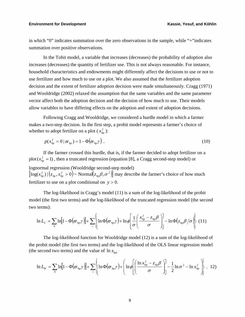
in which “0” indicates summation over the zero observations in the sample, while “+”indicates summation over positive observations.

In the Tobit model, a variable that increases (decreases) the probability of adoption also increases (decreases) the quantity of fertilizer use. This is not always reasonable. For instance, household characteristics and endowments might differently affect the decisions to use or not to use fertilizer and how much to use on a plot. We also assumed that the fertilizer adoption decision and the extent of fertilizer adoption decision were made simultaneously. Cragg (1971) and Wooldridge (2002) relaxed the assumption that the same variables and the same parameter vector affect both the adoption decision and the decision of how much to use. Their models allow variables to have differing effects on the adoption and extent of adoption decisions.

Following Cragg and Wooldridge, we considered a hurdle model in which a farmer makes a two-step decision. In the first step, a probit model represents a farmer’s choice of whether to adopt fertilize on a plot ( f

hpx ):

( )γϖϖ hphpf

hpxp Φ−== 1)|0( . (10)

If the farmer crossed this hurdle, that is, if the farmer decided to adopt fertilizer on a plot )1( =f

hpx , then a truncated regression (equation [8], a Cragg second-step model) or

lognormal regression (Wooldridge second-step model) ( ) ( )[ ]2,Normal~0,|)log( σβhp

fhphp

fhp zxzx > may describe the farmer’s choice of how much

fertilizer to use on a plot conditional on .0>y

The log-likelihood in Cragg’s model (11) is a sum of the log-likelihood of the probit model (the first two terms) and the log-likelihood of the truncated regression model (the second two terms):

( )[ ] ( ) ( )∑ ∑+ ⎪⎭

⎪⎬⎫

⎪⎩

⎪⎨⎧

Φ−⎥⎥⎦

⎤

⎢⎢⎣

⎡⎟⎟⎠

⎞⎜⎜⎝

⎛ −+Φ+Φ−=

0

ln1lnln1lnln σβσ

βσ

φγϖγϖ hphp

fhp

hphpC zzx

L (11)

The log-likelihood function for Wooldridge model (12) is a sum of the log-likelihood of the probit model (the first two terms) and the log-likelihood of the OLS linear regression model (the second two terms) and the value of ln hptx .

( )[ ] ( )∑ ∑+ ⎪⎭

⎪⎬⎫

⎪⎩

⎪⎨⎧

⎟⎟

⎠

⎞

⎜⎜

⎝

⎛−−

⎥⎥⎦

⎤

⎢⎢⎣

⎡⎟⎟⎠

⎞⎜⎜⎝

⎛ −+Φ+Φ−=

0

2 lnln21ln

lnln1lnln fhp

hpf

hphphpW x

zxL σ

σβ

φγϖγϖ . 12)


10

For detailed specification and the estimation procedure of this model, see Wooldridge (2002, 536–38).

The Cragg model has the advantage in that it nests the Tobit model; when hphp z=ϖ and

σβγ = , the Cragg model reduces to the Tobit model log-likelihood function. A likelihood ratio

test can therefore be performed easily to study whether the household fertilizer-use decision on the plot is best modelled by a one-step or a two-step procedure. The difficulty in comparing the Wooldridge model versus the Cragg model is that they do not nest in each other. The same is true for the Tobit model and the Wooldridge model. We used Voung’s (1989) non-nested model-selection test.

The log-likelihood ratio test (LR) can be used to test a model which is nested in a more general model. It can be done by testing the hypothesis that the restrictions can be statistically accepted or not. The Tobit model is tested against the Cragg model by performing a likelihood ratio test of the following:

)lnln(ln2 Tobitegressiontruncatedrprobit LLLL −+= , (13)

where L is distributed as a chi-square with k degree of freedom ( K is the number of independent variables including a constant). The null hypothesis is the Tobit model (restricted model), with the log-likelihood function given in equation (9), and the alternative model (unrestricted) is the Cragg’s model (probit and a truncated regression estimated separately), with a log-likelihood function given in equation (11). The Tobit model will be rejected in favor of Cragg’s model, if L exceeds the chi-square critical value. The likelihood ratio test statistics of [ 2(43) 707.99, 0.000)chi p= = indicated that the restrictions imposed by the Tobit model were

rejected in favor of Cragg’s model. The same household and farm characteristics did not have equal influence on both the adoption decision and the decision of how much fertilizer to use on a plot. It also implied that the fertilizer adoption decision and the extent of fertilizer adoption decision were not made simultaneously. Hypothesizing whether a given variable has impact on the adoption decision—but not on the extent of the adoption decision, or vice versa—is difficult. Consequently, the three models were estimated with the same variables.

The Cragg and Tobit model can be compared to the Wooldridge model using the Voung non-nested model specification test. Based on Kullback-Leibler information criterion, Voung (1989) proposed the following statistics under regularity conditions for strictly non-nested models:

=V )1,0(ˆ)ˆ,ˆ(21 NLRn nnnn →− ωυθ , (14)


11

where )ˆ,ˆ( nnnLR υθ is the difference between the log-likelihood values for two models, and nθ̂ and nυ̂ are the maximum likelihood estimators from the two models, respectively. ˆ nϖ is defined

as:

,)ˆ;()ˆ;(

log1)ˆ;()ˆ;(

log1ˆ2

1

2

1

2

⎥⎥⎦

⎤

⎢⎢⎣

⎡

|

|−

⎥⎥⎦

⎤

⎢⎢⎣

⎡

|

|= ∑∑

==

n

i nhphp

nhphpn

i nhphp

nhphpn xyg

xyfnxyg

xyfn υ

θυθ

ω

where n is the number of observations. The null hypothesis was that the two models equally fit the data. We rejected the null hypothesis and accepted model ˆf

θ (Wooldridge or lognormal

model), when V is higher than c (critical value from a standard normal distribution for some significance level) and rejected the null and accepted model v̂g (Tobit or Cragg regression model), when V is smaller than c− . If V c≤ , the two models cannot be discriminated, given

the data. (See details in Voung 1989.) The Voung test statistic is asymptotically distributed as standard normal distribution.

The Voung test statistic accepts that the Cragg model dominates the Wooldridge model ( -16.52)V = . Comparing the Wooldridge and Tobit model, the Tobit model better fits the data ( -6.48)V = . The critical values )(c for the 1- and 5-percent significance level are 2.58 and 1.96,

respectively. The production risk impact on fertilizer use, therefore, is presented based on the Cragg model.

4.2. Econometric Estimation Challenges and Remedies

To obtain consistent estimates of production risk impact on technology adoption, we needed to control for unobserved heterogeneity ( htu ) that might be correlated with observed

explanatory variables. One way to address this issue was to exploit the panel nature of our plot-level data and use household-specific fixed effects. The household fixed effects could be used for estimation of linear models (for estimation of first, second, and third moments). Unfortunately, non-linear maximum likelihood models (e.g., Probit, truncated, and Tobit regression models) cannot be directly estimated using fixed effects models because of the incidental parameters problem (Wooldridge 2002; Hsiao 2003). As a result, it was difficult to handle the unobserved effects. As an alternative, we used modified probit random effects and pooled truncated regression models, where the right hand-side of each regression equation included the mean value of the plot-varying explanatory variables following Mundlak’s (1978) approach. Mundlak’s approach relies on the assumption that unobserved effects are linearly correlated with explanatory variables as specified by:


12

hh x ηαψ += , )iid(0,~ 2ησηh , (15)

where x is the mean of the plot-varying explanatory variables within each household (cluster mean), α is the corresponding vector coefficient, and η is a random error unrelated to sx ' . In

our case, it was most important to include average plot characteristics, such as average plot fertility, soil depth, plot slope, and conventional input use, which we believed had heavy impacts on production and technology adoption decisions. The vector α will be equal to zero if the observed explanatory variables are uncorrelated with the random effects.

The use of fixed effects techniques and Mundlak’s approach also helped address the problem of selection (related to technology adoption and risk management) and endogeneity bias, if the selection and endogeneity bias are due to plot-invariant unobserved factors, such as household heterogeneity (Wooldridge 2002). However, if the unobserved plot component )( hpe

is correlated with the decision to adopt technology, the parameter estimates of each regression equation would be inconsistent. If we failed to control for these factors, we would not obtain the true effect of conservation. Controlling for plot heterogeneity was a bit more difficult than addressing household heterogeneity. Fortunately, our dataset offered a richer characterization of plot quality than found in most of the other studies. It was likely that observed plot quality would be positively correlated with unobserved plot quality. In terms of plot characteristics, the data set included plot slope, plot size, soil fertility, soil depth, plot distance from the homestead, altitude, and input use. Including these variables in our model allowed us to address selection due to idiosyncratic errors (e.g., plot heterogeneity), using observed plot quality characteristics and inputs (Fafchamps 1993; Levinsohn and Petrin 2003; Assunção and Braido 2004). The use of input use to control for plot heterogeneity was based on the notion that farmers might respond to positive and negative shocks by increasing or decreasing their input use.

In the empirical model, variables such as inputs (e.g., fertilizer use and improved seed use per ha) were potentially endogenous variables. We did not believe this to be a problem, however, because explanatory variables explaining input use were also included. In addition, our estimation approaches (fixed effects and modified random effects) helped control for unobserved effects that might correlate with input use decisions.

5

5 Traditionally, farm households retain their own seeds from the previous harvest for use in the following season. Seed use, therefore, is a pre-determined variable. Improved seeds were used only on 5.6 percent of the sample plots (3369). We assumed labor and oxen use were fixed in the short-term, since households usually depended on family resources because of limited labor and oxen markets.


13

Finally, endogeneity of other explanatory variables such crop types might bias model results. However, crop compositions including different varieties (multiple traditional and improved varieties) are among those strategies used by developing countries farmers to deal with production risk (Fafchamps 1993). Crop choice might also be correlated with unobserved plot attributes, and with their inclusion, bias due to unobserved plot attributes might have been reduced. Besides these, the cropping pattern was stable in the village where similar crops are grown year after year based on crop rotation and preference of own product for household consumption. Thus, crop choices could be considered as pre-determined variables both in production function and adoption model. However, we hoped that any systematic decision of the choice of crops by the household could be captured by the household fixed-effects procedure, Mundlak’s approach, and the variables included in each model (e.g., plot characteristics and labor use).

5. Data Sources and Types

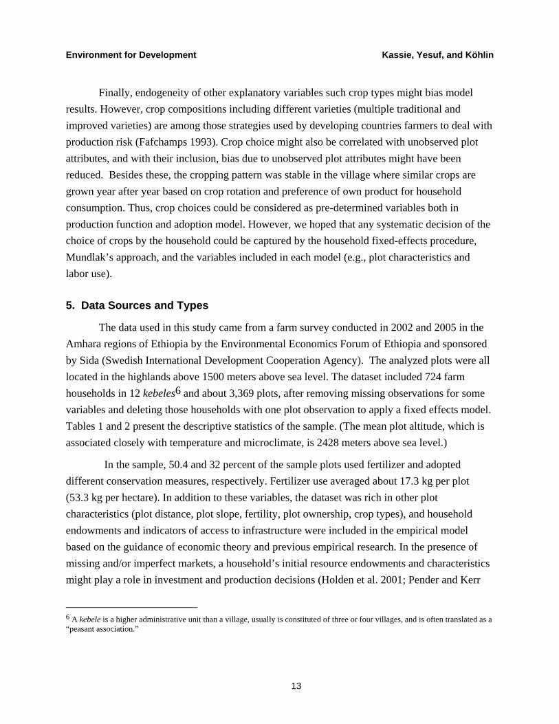
The data used in this study came from a farm survey conducted in 2002 and 2005 in the Amhara regions of Ethiopia by the Environmental Economics Forum of Ethiopia and sponsored by Sida (Swedish International Development Cooperation Agency). The analyzed plots were all located in the highlands above 1500 meters above sea level. The dataset included 724 farm households in 12 kebeles6 and about 3,369 plots, after removing missing observations for some variables and deleting those households with one plot observation to apply a fixed effects model. Tables 1 and 2 present the descriptive statistics of the sample. (The mean plot altitude, which is associated closely with temperature and microclimate, is 2428 meters above sea level.)

In the sample, 50.4 and 32 percent of the sample plots used fertilizer and adopted different conservation measures, respectively. Fertilizer use averaged about 17.3 kg per plot (53.3 kg per hectare). In addition to these variables, the dataset was rich in other plot characteristics (plot distance, plot slope, fertility, plot ownership, crop types), and household endowments and indicators of access to infrastructure were included in the empirical model based on the guidance of economic theory and previous empirical research. In the presence of missing and/or imperfect markets, a household’s initial resource endowments and characteristics might play a role in investment and production decisions (Holden et al. 2001; Pender and Kerr

6 A kebele is a higher administrative unit than a village, usually is constituted of three or four villages, and is often translated as a “peasant association.”


14

1998) and were therefore included. In addition, location dummy variables were also collected to capture the impact of different infrastructure and rainfall on technology adoption and production decisions.

Table 1 Summary Statistics of Variables for Fertilizer Adoption

Variables All sample plots

Fertilized plots

Non-fertilized plots

Value of crop production per plot (ETB)

501.873 (910.011)

600.006 (1188.172)

402.286 (465.428)

Plot size, hectare 0.344

(0.256) 0.354

(0.226) 0.333

(0.283)

Labor use per plot (days) 43.754

(85.218) 44.862

(108.238) 42.629

(52.388)

Oxen use per plot (days) 5.602

(5.230) 6.696

(5.638) 4.492

(4.518)

Fertilizer use per plot (kg) 17.139

(25.619) 34.027

(26.991)

Seed use per plot (kg) 31.614

(30.586) 35.709

(32.161) 27.459

(28.311)

Manure use per plot (dummy) 82.128

(273.928) 47.407

(213.240) 117.362

(320.340)

Improved seed use (dummy) 0.056 0.092 0.021

Gently slopped plots (dummy) 0.655 0.645 0.664

Mid-hill sloped plots (dummy) 0.282 0.296 0.276

Steep hill slopped plots (dummy) 0.059 0.059 0.059

High fertile plots (dummy) 0.321 0.260 0.383

Medium fertile plots (dummy) 0.437 0.454 0.420

Poor fertile plots (dummy) 0.242 0.286 0.197

Irrigated plots (dummy) 0.277 0.341 0.212

Conserved plots (dummy) 0.321 0.249 0.394

Plot distance to residence (walking minutes)

15.016 (17.515)

15.547 (17.287)

14.477 (17.733)

Plot altitude (m.a.s.l.) 2428.306 (131.090)

2413.381 (129.545)

2443.452 (130.949)

Rented in plots (dummy) 0.008 0.008 0.008

Residence distance to town (walking minutes)

62.418 (38.818)

64.678 (39.225)

61.445 (38.558)


15


Fertilized plots

Non-fertilized plots

Residence distance to road (walking minutes)

35.936 (30.597)

39.232 (30.426)

35.636 (30.329)

Household age (years) 48.494

(14.160) 47.557

(14.270) 48.657

(14.143)

Livestock holding (TLU) 4.418

(3.040) 4.908

(3.107) 4.423

(3.113)

Total number of family members 6.452

(2.241) 6.517

(2.206) 6.454

(2.282)

Number of plots farmed 8.519

(4.050) 9.625

(4.108) 8.630

(4.091)

Number of plot observations 3399 1712 1687

Number of household observations 724 480 638

Standard deviations are in parentheses. m.a.s.l. = meters above sea level TLU = tropical livestock units

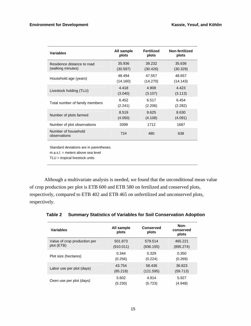
Although a multivariate analysis is needed, we found that the unconditional mean value of crop production per plot is ETB 600 and ETB 580 on fertilized and conserved plots, respectively, compared to ETB 402 and ETB 465 on unfertilized and unconserved plots, respectively.

Table 2 Summary Statistics of Variables for Soil Conservation Adoption


Conserved plots

Non-conserved

plots

Value of crop production per plot (ETB)

501.873 (910.011)

579.514 (936.155)

465.221 (895.274)

Plot size (hectares) 0.344

(0.256) 0.329

(0.224) 0.350

(0.269)

Labor use per plot (days) 43.754

(85.218) 58.436

(121.595) 36.823

(59.713)

Oxen use per plot (days) 5.602

(5.230) 4.914

(5.723) 5.927

(4.948)


16


Conserved plots

Non-conserved

plots

Fertilizer use per plot (kg) 17.139

(30.586) 13.070

(24.352) 19.059

(32.786)

Manure use per plot (kg) 82.128

(273.928) 97.863

(269.181) 74.699

(275.886)

Improved seed use (dummy) 0.056 0.055 0.057

Gently slopped plots (dummy) 0.655 0.528 0.715

Mid-hill sloped plots (dummy) 0.286 0.387 0.239

Steep hill slopped plots (dummy) 0.059 0.085 0.047

High fertile plots (dummy) 0.321 0.374 0.296

Medium fertile plots (dummy) 0.437 0.433 0.440

Poor fertile plots (dummy) 0.242 0.192 0.265

Irrigated plots (dummy) 0.277 0.022 0.398

Rented in plots (dummy) 0.008 0.006 0.009

Conserved plots (dummy) 0.321

Plot distance to residence (walking minutes)

15.016 (17.515)

13.555 (16.440)

15.706 (17.963)

Plot altitude (m.a.s.l.) 2428.306 (131.090)

2454.580 (115.953)

2415.903 (135.928)

Residence distance to town (walking minutes )

62.418 (38.818)

64.086 (40.237)

61.944 (38.846)

Residence distance to road (walking minutes)

35.936 (30.597)

32.641 (29.923)

38.286 (31.367)

Household age (years) 48.494

(14.160) 48.845

(14.160) 48.481

(14.478)

Number of livestock (TLU) 4.418

(3.040) 4.043

(2.746) 4.639

(3.165)

Total number of family members 6.452

(2.241) 6.533

(2.310) 6.460

(2.238)

Number of plots operated 8.519

(4.050) 7.803

(3.807) 9.109

(4.136)


Number of household observations 724 432 577

Standard deviations are in parentheses. ETB = Ethiopian birr (unit of currency). m.a.s.l. = meters above seal level. TLU = tropical livestock unit


17

6. Results and Discussion

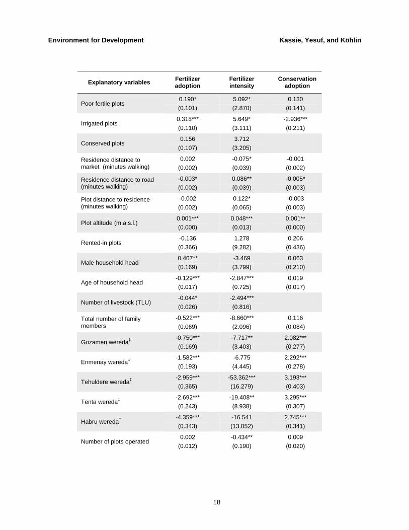
Table 3 presents the results of the determinants of fertilizer and conservation adoption. In the interest of space and brevity, the econometrics results (fixed effects results) for the mean function, variance function, and skewness function are not reported, but are available from the authors. In the case of soil conservation adoption, we estimated only the likelihood of adoption, using a modified random effects model. Otherwise, both the probability and the extent of fertilizer adoptions were estimated using modified random effects probit model and modified pooled truncated regression model.

Bootstrapped standard errors are used to obtain consistent estimates since we used generated regressors (i.e., value of crop production moments) in the estimation of production risk impact on fertilizer and conservation adoption model. The empirical results showed that there was a correlation between the observed explanatory variables and unobserved effects (table 3), implying that ignoring this might lead to biased estimates of production risk impact on technology adoption.

Table 3 Determinants of Fertilizer and Soil Conservation Adoption

Explanatory variables Fertilizer adoption

Fertilizer intensity

Conservation adoption

Predicted mean yield 1.346*** (0.087)

36.235*** (3.584)

0.587*** (0.091)

Predicted variance of yield -0.297*** (0.109)

-4.870** (2.151)

0.263 (0.166)

Predicted skewness of yield -0.217*** (0.043)

-5.996*** (1.836)

0.024 (0.068)

Ln (plot size) -0.434*** (0.074)

12.809*** (2.382)

-0.208** (0.091)

Manure use -0.001*** (0.000)

-0.001 (0.004)

0.000 (0.000)

Improved seed use 1.348*** (0.195)

8.604*** (2.949)

Medium sloped plots 0.094

(0.085) 3.078

(2.545) 0.770*** (0.109)

Steeply sloped plots -0.082 (0.148)

0.634 (4.502)

0.920*** (0.206)

Medium fertile plots 0.011

(0.087) 2.432

(2.390) 0.069

(0.111)


18




Poor fertile plots 0.190* (0.101)

5.092* (2.870)

0.130 (0.141)

Irrigated plots 0.318*** (0.110)

5.649* (3.111)

-2.936*** (0.211)

Conserved plots 0.156

(0.107) 3.712

(3.205)

Residence distance to market (minutes walking)

0.002 (0.002)

-0.075* (0.039)

-0.001 (0.002)

Residence distance to road (minutes walking)

-0.003* (0.002)

0.086** (0.039)

-0.005* (0.003)

Plot distance to residence (minutes walking)

-0.002 (0.002)

0.122* (0.065)

-0.003 (0.003)

Plot altitude (m.a.s.l.) 0.001*** (0.000)

0.048*** (0.013)

0.001** (0.000)

Rented-in plots -0.136 (0.366)

1.278 (9.282)

0.206 (0.436)

Male household head 0.407** (0.169)

-3.469 (3.799)

0.063 (0.210)

Age of household head -0.129*** (0.017)

-2.847*** (0.725)

0.019 (0.017)

Number of livestock (TLU) -0.044* (0.026)

-2.494*** (0.816)

Total number of family members

-0.522*** (0.069)

-8.660*** (2.096)

0.116 (0.084)

Gozamen wereda‡ -0.750*** (0.169)

-7.717** (3.403)

2.082*** (0.277)

Enmenay wereda‡ -1.582*** (0.193)

-6.775 (4.445)

2.292*** (0.278)

Tehuldere wereda‡ -2.959*** (0.365)

-53.362*** (16.279)

3.193*** (0.403)

Tenta wereda‡ -2.692*** (0.243)

-19.408** (8.938)

3.295*** (0.307)

Habru wereda‡ -4.359*** (0.343)

-16.541 (13.052)

2.745*** (0.341)

Number of plots operated 0.002

(0.012) -0.434** (0.190)

0.009 (0.020)


19




Mean of plot varying 121.05*** 76.11*** 16.78

Constant -13.935***

1.966) -263.020***

(62.688) -5.193** (2.583)

Wald chi2(42) 466.885 301.691 409.750


* p<0.10, ** p<0.05, *** p<0.01 ‡ A wereda (or woreda) is an administrative district of local government in Ethiopia, made up of kebeles (neighborhood or peasant associations). Weredas are typically collected together (usually contiguous weredas) into zones.

The fertilizer estimation results revealed that the explanatory variables had a different impact on the decision to use and how much to use. This is in line with the empirical evidence reported in section three. Production risks have a central role in the decision to adopt fertilizer and extent of fertilizer use. The first and second, and third moments, respectively, have a positive and a negative significant impact on the decision to use and how much to use. The higher the expected return, the greater the probability of adopting fertilizer and the greater the extent of fertilizer uses. On the other hand, the higher the variance of return and probability of crop failure (downside risk) were, the lower the probability to adopt fertilizer and the lower the extent of fertilizer uses were. The implication is that mechanisms that reduce variance of return and exposure to downside risk and insure that food production would not fall below some threshold level are desirable in the fertilizer adoption.

In addition to the production-risk variables, plot-level (e.g., irrigated plots, plot altitude, plot size, manure use) and household-level (e.g., family size, and household age) variables and location dummies had a statistically significant impact on the decision to adopt and extent of adoption.

Unlike fertilizer adoption, conservation adoption was not significantly affected by risk exposure, including downside risk. However, expected return increased adoption, implying that farm households expected higher returns if they adopted conservation technology. Kassie et al. (2007) in the same study area found that stone bunds had no statistically significant impact on crop production, implying low adoption rates of stone bunds in the study area. In addition to expected return, plot level variables (e.g., plot size, irrigated plots, and plot slope and altitude) and location dummies significantly affected conservation adoption.


20

7. Summary and Conclusion

This paper, using a moment-based approach, empirically examined the relationship between production risk and adoption of sustainable land-management technologies. A modified random-effects probit model to estimate fertilizer and conservation adoption and a modified truncated regression model to estimate the extent of fertilizer were used. Two-year cross-sectional plot level data were used. Econometrics results revealed that production risk (as measured by the variability of return and crop failure) negatively affected the decision to use and the extent of adoption of chemical fertilizer. Production risks, on the other hand, had no statistical significance impact on conservation adoption. However, the expected return had a positive and significant impact on both fertilizer and conservation adoption.

This study has the following important policy implications. First, the impact of production risk varies by technology type. Production risk affects fertilizer adoption, but not conservation adoption. Second, when considering promoting the adoption of fertilizer, neglecting risk (particularly for risk-averse farmers) could lead to the formulation of wrong policies. Without considering risk, a sub-optimal (low) use of fertilizer might be associated with inefficient allocation of fertilizer by farmers, since for risk-averse farmers, the marginal value of variable inputs exceeded their market price. Third, economic instruments to hedge against exposure to risk (e.g., a properly designed safety net program) are desirable to reduce poverty through adoption of improved technologies.


21

References

Abrar, S., O. Morrissey, and T. Rayner. 2004. “Crop-Level Supply Response by Agro-Climatic Region in Ethiopia,” Journal of Agricultural Economics 55(2): 289–311.

Alemu, T. 1999. “Land Tenure and Soil conservation: Evidence from Ethiopia.” PhD thesis. Department of Economics, University of Gothenburg, Sweden.

Asfaw, A., and A. Admassie. 2004. “The Role of Education on the Adoption of Chemical Fertiliser under Different Socio-Economic Environments in Ethiopia,” Agricultural Economics 30: 215–28.

Assunção, J. J., and L.H.B Braido. 2004. “Testing Competing Explanations for the Inverse Productivity Puzzle.” Unpublished manuscript. Department of Economics, Pontifical Catholic University of Rio de Janeiro, Brazil.

Antle, J.M. 1983. Testing for Stochastic Structure of Production: A Flexible Moment-Based Approach, Journal of Business and Economic Statistics 1(3): 192–201.

Antle, J.M., and W.J. Goodger. 1984. “Measuring Stochastic Technology: The Case of Tulare Milk Production,” American Journal of Agricultural Economics 66: 342–50.

Antle, J. 1987. “Econometric Estimation of Producers' Risk Attitudes,” American Journal of Agricultural Economics 69(3): 509–522.

Benin, S., and J. Pender. 2001. “Impacts of Land Redistribution on Land Management and Productivity in the Ethiopian Highlands,” Land Degradation and Development 12: 555–68.

Binswanger, H.P. 1981. “Attitudes Toward Risk: Theoretical Implications of an Experiment in Rural India,” The Economic Journal 91: 867–90.

Chavas, J.P., and M.T. Holt. 1996. “Economic Behavior under Uncertainty: A Joint Analysis of Risk Preferences and Technology,” Review of Economics and Statistics 78, 329–35.

Christiaensen, L., and L. Demery. 2007. Down to Earth: Agriculture and Poverty Reduction in Africa. Directions in Development—Poverty series. Washington DC: World Bank.

Croppenstedt, A., M. Demeke, and M. Meschi. 2003. “Technology Adoption in the Presence of Constraints: The Case of Fertilizer Demand in Ethiopia,” Review of Development Economics 7(1): 58–70.


22

Cragg, J. 1971. “Some Statistical Models for Limited Dependent Variables with Application to the Demand for Durable Goods,” Econometrica 39(5): 829–44.

Dadi, L., M. Burton, and A. Ozanne. 2004. “Duration Analysis of Technology Adoption in Ethiopian Agriculture,” Journal of Agricultural Economics 55(3): 613–31.

Deininger K., S. Jin, B. Adenew, S. Gebre-Selassie, and B. Nega. 2003. Tenure Security and Land-Related Investment: Evidence from Ethiopia.” Policy Research Working Paper, no. 2991. Washington, DC: World Bank. http://www-wds.worldbank.org/servlet/WDSContentServer/WDSP/IB/2003/04/11/000094946_03032704080562/additional/128528322_20041117164103.pdf. Accessed February 10, 2008.

Dercon, S. 2004. “Growth and Shocks: Evidence from Rural Ethiopia,” Journal of Development Economics 74(2): 309–329.

Dercon, S., and L. Christiaensen. 2007. “Consumption Risk, Technology Adoption, and Poverty Traps: Evidence from Ethiopia.” Policy Research Working Paper, no. 4257. Washington, DC: World Bank. http://www-wds.worldbank.org/servlet/WDSContentServer/WDSP/IB/2007/06/15/000016406_20070615145611/Rendered/PDF/wps4257.pdf. Accessed February 10, 2008.

Di Falco, S., and Chavas, J.P. 2006. “Production Risk, Food Security and Crop Biodiversity:Evidence from Barley Production in the Tigray Region, Ethiopia.” Online paper. University College London. www.ucl.ac.uk/bioecon/9th%20paper/DiFalco.pdf. Accessed February 10, 2008.

Ersado L., G. Amacher, and J. Alwang. 2003. “Productivity and Land Enhancing Technologies in Northern Ethiopia: Health, Public Investments and Sequential Adoption.” Environment and Production Technology Division Discussion Paper, no. 102. Washington, DC: International Food Policy Research Institute.

Fafchamps, M. 1993. “Sequential Labour Decisions under Uncertainty: An Estimable Household Model of West Africa Farmers.” Econometrica 61: 1173–97.

Feder, G., and L.D. Umal. 1990. “The Adoption of Agricultural Innovations: A Review,” Technological Forecasting and Social Change 43: 215–39.

Fin, T., and P. Schmidt. 1984. “A Test of the Tobit Specification against an Alternative Suggested by Cragg,” Review of Economics and Statistics 66: 174–77.


23

Gebremedhin, B., and M. Swinton. 2003. “Investment in Soil Conservation in Northern Ethiopia: The Role of Land Tenure Security and Public Programs,” Agricultural Economics 29: 69–84.

Grepperud, S. 1996. “Population Pressure and Land Degradation: The Case of Ethiopia,” Journal of Environmental Economics and Management 30: 18–33.

Hagos, F. 2003. “Poverty, Institutions, Peasant Behavior and Conservation Investment in Northern Ethiopia.” PhD dissertation, no. 2003:2, Department of Economics and Social Sciences, Agricultural University of Norway, Ås, Norway.

Holden, S.T., and B. Shiferaw. 2004. Land Degradation, Drought, and Food Security in a Less-Favoured Area in the Ethiopian Highlands: A Bio-economic Model with Market Imperfections,” Agricultural Economics 30 (1): 31–49.

Holden, S.T., Shiferaw, B. and Pender, J. 2001. “Market Imperfections and Profitability of Land Use in the Ethiopian Highlands: A Comparison of Selection Models with Heteroskedasticity,” Journal of Agricultural Economics 52(2): 53–70.

Holden, S.T., and H. Yohannes. 2002. “Land Redistribution, Tenure Insecurity, and Input Intensity: A Study of Farm Households in Southern Ethiopia,” Land Economics 78: 573–90.

Just, R., and R. Pope. 1979. “Production Function Estimation and Related Risk Considerations,” American Journal of Agricultural Economics 61(2): 276–84.

Kim, K., and P.J. Chavas. 2003. “Technological Change and Risk Management: An Application to the Economics of Corn Production,” Agricultural Economics 29: 125–42.

Koundouri P., C. Nauges, and V. Tzouvelekas. 2006. “Technology Adoption under Production Uncertainty: Theory and Application to Irrigation Technology,” American Journal of Agricultural Economics 8(3): 657–70.

Levinsohn, J., and A. Petrin. 2003. “Estimating Production Functions Using Inputs to Control for Unobservables,” Review of Economic Studies 70: 317–41.

Morris, M., Kelly V.A., R.J. Kopicki, and D. Byerlee. 2007. Fertilizer Use in African Agriculture: Lessons Learned and Good Practice Guidelines. Directions in Development—Agriculture and Rural Development series. World Bank: Washington D.C. http://www-wds.worldbank.org/external/default/WDSContentServer/WDSP/IB/2007/03/15/00031060


24

7_20070315153201/Rendered/PDF/390370AFR0Fert101OFFICIAL0USE0ONLY1.pdf. Accessed February 10, 2008.

Mosley, P., and A. Verschoor. 2005. “Risk Attitudes and the Vicious Circle of Poverty,” European Journal of Development Research 17(1): 55–88.

Mulat, D., S. Ali, and T. Jayne. 1997. “Promoting Fertilizer Use in Ethiopia: The Implications of Improving Grain Market Performance, Input Market Efficiency, and Farm Management.” Working Paper 5. Grain Market Research Project, Ministry of Economic Development and Cooperation, Addis Ababa, Ethiopia.

Mundlak, Y. 1978. On the Pooling of Time Series and Cross-Section Data. Econometrica 46: 69–85.

Pender, J., and M. Fafchamps. 2006. “Land Lease Markets and Agricultural Efficiency in Ethiopia,” Journal of African Economies 15(2): 251–84.

Pender, J., and B. Gebremedhin. 2006. Impacts of Policies and Technologies in Dryland Agriculture: Evidence from Northern Ethiopia. In Challenges and Strategies for Dryland Agriculture, edited by S.C. Rao and J. Ryan, CSSA Special Publication 32. Madison, WI: American Society of Agronomy and Crop Science Society of America.

Pender, J., B. Gebremedhin, and M. Haile. 2003. “Livelihood Strategies and Land Management Practices in the Highlands of Tigray.” Paper (revised) presented at the “Policies for Sustainable Land Management in the East African Highlands” conference, United Nations Economic Commission for Africa, Addis Ababa, Ethiopia, April 24–26, 2002. Washington, DC: International Food Policy Research Institute.

Pender, J.P., and M.J. Kerr. 1998. “Determinants of Farmer’s Indigenous Soil and Water Conservation Investments in Semi-Arid India,” Agricultural Economics 19: 113–25.

Rosenzweig, M., and H. Binswanger.1993. “Wealth, Weather Risk, and the Composition and Profitability of Agricultural Investments,” Economic Journal 103(416): 56–78.

Shiferaw, B., and Holden, S.T. 1998. Resource Degradation and Adoption of Land Conservation Technologies in the Ethiopian Highlands: A Case Study in Andit Tid, North Shewa,” Agricultural Economics 18: 233–47.

Voung, Q.H. 1989. “Likelihood Ratio Tests for Model Selection and Non-nested Hypothesis,” Econometrica 57: 307–333.


25

Wooldridge, J. M. 2002. Econometric Analysis of Cross Section and Panel Data. Cambridge, MA: MIT Press.

World Bank. 2006. “Ethiopia: Policies for Pro-Poor Agricultural Growth, Africa Region.” Photocopy. Washington DC: World Bank.

Yesuf, M. 2004. “Risk, Time, and Land Management under Market Imperfection: Applications to Ethiopia.” PhD thesis. Department of Economics, University of Gothenburg, Sweden.

the role of production risk in sustainable land ... sustainable land- management technology adoption...

Documents