adoption and impact of improved groundnut varieties on ... · adoption and impact of improved...

Environment for Development

Discussion Paper Series May 2010 EfD DP 10-11

Adoption and Impact of Improved Groundnut Varieties on Rural Poverty

Evidence from Rural Uganda

Mena le Kass ie , Beke le Sh i fe raw , and Geof f re y Mur ic ho

Environment for Development

The Environment for Development (EfD) initiative is an environmental economics program focused on international research collaboration, policy advice, and academic training. It supports centers in Central America, China, Ethiopia, Kenya, South Africa, and Tanzania, in partnership with the Environmental Economics Unit at the University of Gothenburg in Sweden and Resources for the Future in Washington, DC. Financial support for the program is provided by the Swedish International Development Cooperation Agency (Sida). Read more about the program at www.efdinitiative.org or contact [email protected].

Central America Environment for Development Program for Central America Centro Agronómico Tropical de Investigacíon y Ensenanza (CATIE) Email: [email protected]

China Environmental Economics Program in China (EEPC) Peking University Email: [email protected]

Ethiopia Environmental Economics Policy Forum for Ethiopia (EEPFE) Ethiopian Development Research Institute (EDRI/AAU) Email: [email protected]

Kenya Environment for Development Kenya Kenya Institute for Public Policy Research and Analysis (KIPPRA) Nairobi University Email: [email protected]

South Africa Environmental Policy Research Unit (EPRU) University of Cape Town Email: [email protected]

Tanzania Environment for Development Tanzania University of Dar es Salaam Email: [email protected]

© 2010 Environment for Development. All rights reserved. No portion of this paper may be reproduced without permission of the authors.

Discussion papers are research materials circulated by their authors for purposes of information and discussion. They have not necessarily undergone formal peer review.

Adoption and Impact of Improved Groundnut Varieties on Rural Poverty: Evidence from Rural Uganda

Menale Kassie, Bekele Shiferaw, and Geoffrey Muricho

Abstract This paper evaluates the ex-post impact of adopting improved groundnut varieties on crop

income and rural poverty in rural Uganda. The study utilizes cross-sectional farm household data collected in 2006 in seven districts of Uganda. We estimated the average adoption premium using propensity score matching (PSM), poverty dominance analysis tests, and a linear regression model to check robustness of results. Poverty dominance analysis tests and linear regression estimates are based on matched observations of adopters and non-adopters obtained from the PSM. This helped us estimate the true welfare effect of technology adoption by controlling for the role of selection problem on production and adoption decisions. Furthermore, we checked covariate balancing with a standardized bias measure and sensitivity of the estimated adoption effect to unobserved selection bias, using the Rosenbaum bounds procedure. The paper computes income-based poverty measures and investigates their sensitivity to the use of different poverty lines. We found that adoption of improved groundnut technologies has a significant positive impact on crop income and poverty reduction. These results are not sensitive to unobserved selection bias; therefore, we can be confident that the estimated adoption effect indicates a pure effect of improved groundnut technology adoption.

Key Words: groundnut technology adoption, crop income, poverty alleviation, propensity

score matching, switching regression, stochastic dominance, Rosenbaum bounds, Uganda

JEL Classification: C01, C21, I32, O12, Q16

Contents

Introduction ............................................................................................................................. 1

1. Econometric Framework .................................................................................................... 3

1.1 Propensity Score Matching Method ............................................................................. 4

1.2 Parametric Regression Analysis .................................................................................. 8

1.3 Poverty Measures and Stochastic Dominance ........................................................... 10

2. Data Source and Descriptive Statistics ........................................................................... 12

3. Results of Estimation of Propensity Score ...................................................................... 16

4. Estimation of Treatment Effect: Matching Algorithms .............................................. 20

5. Estimation of Average Treatment Effect: Switching Regression Approach ............. 23

6. Estimation of Groundnut Adoption Impact on Poverty Alleviation ........................... 23

7. Summary and Conclusion ................................................................................................ 26

References .............................................................................................................................. 28

Environment for Development Kassie, Shiferaw, and Muricho

1

Adoption and Impact of Improved Groundnut Varieties on Rural Poverty: Evidence from Rural Uganda

Menale Kassie, Bekele Shiferaw, and Geoffrey Muricho∗

Introduction

At the Millennium Summit in 2000, the international community agreed to halve by 2015 the proportion of people living on less than US$ 1 a day.1 Poverty in sub-Saharan Africa particularly has remained stubbornly high throughout the past two decades. The share of people living on less than $1 a day in this region exceeds that in the next poorest region of South Asia by about 17%. As of 2002, the number of people living in poverty was much higher than 1973, while the poverty rate remained virtually constant at 44% (ECA 2007). Approximately 90% of the so-called “bottom billion”—a large portion of whom live in sub-Saharan Africa—inhabit rural areas and virtually all of these rely on agriculture for their food and incomes (Collier 2007; World Bank 2008). Agriculture, indeed, accounts for more than 30% of Africa’s gross domestic product (GDP) and 75% of total employment.

The path out of the poverty trap in these countries, therefore, depends on the growth and development of the agricultural sector. It is important for a number of reasons: 1) to alleviate poverty through income generation and employment creation; 2) to meet growing food needs driven by rapid population growth; 3) to keep food prices low, both for urban households and the many rural households who are net food buyers; 4) to stimulate overall economic growth in agriculture-based economies; and 5) to conserve natural resources2 (Pinstrup-Andersen and Pandya-Lorch 1995; de Janvry and Sadoulet 2001; Alwang and Siegel 2003; Moyo et al. 2007).

Agricultural growth and development, and consequent reduction of poverty, are not possible without yield-enhancing technical options because it is no longer possible (except in a

∗ Menale Kassie, Department of Economics, University of Gothenburg, Box 640, SE 405 30, Gothenburg, Sweden, (email) [email protected]; Bekele Shiferaw, International Maize and Wheat Improvement Center (CIMMYT), Box 1041, Nairobi, Kenya, (email) [email protected]; Geoffrey Muricho, International Maize and Wheat Improvement Center (CIMMYT), Box 1041, Nairobi, Kenya, (email) [email protected]. 1 September 6–8, 2000. See “Key Proposals,” “Freedom from Want: Poverty,” on the Millennium Assembly website, http://www.un.org/millennium/sg/report/key.htm. 2 Because the poor lack alternative means to intensify agriculture, they are forced to overuse or misuse natural resource to meet basic needs.


2

few areas) to meet the needs of increasing numbers of people by expanding areas under traditional cultivation. Agricultural research and technological improvements are therefore crucial to increase agricultural productivity and reduce poverty, and meet demands for food at reasonable prices without irreversible degradation of the natural resource base. In recent years, policymakers asked that research managers explicitly consider poverty reduction objectives when setting priorities and making resource allocations (Alwang and Siegel 2003; Moyo et al. 2007). In response, international and national agricultural research centers are investing a substantial amount of resources to respond to such demand. For instance, the International Crops Research Institute for Semi-Arid Tropics (ICRISAT), together with its partners, is developing and disseminating a number of high-yielding, well-adapted, improved cultivars of dryland legumes with market-preferred traits, such as groundnuts that are widely grown in many parts of sub-Saharan Africa.

The main objective of such development research is to reduce hunger, malnutrition, and poverty, and increase the incomes of poor people living in drought-prone areas. However, despite the progress made in delivering innovations to smallholder farmers, there is little empirical research relating technology adoption to poverty reduction. This is mainly due to lack of appropriate methods to link adoption with poverty, and most previous research has failed to move beyond estimating the economic surplus and return to research investment.

A major drawback of the few studies that have attempted to evaluate the impacts of adopting improved technologies is that they do not properly control for potential differences between technology adopters (participants) and farmers in the comparison group (non-adopters or non-participants), making it difficult to draw definitive conclusions (e.g., Rahman 1999; Mendola 2007). Direct comparison of different outcomes between adopters and non-adopters would be statistically misleading for many reasons. First, farmers who adopt the technology are likely to be different from the non-adopters in ways that are unobserved to the researcher. For example, if more motivated farmers are more likely to be selected, then comparing adopters to non-adopters would overestimate the technology’s impact on farm-level outcomes. Second, individuals might be chosen by policymakers or development agencies based on their propensity to participate in technology adoption. In the absence of non-random selection of farm households in technology adoption studies with controls, simple comparisons of outcome measures between adopters and non-adopters is likely to yield biased estimates of technology adoption impact.

Recent studies that employ an ex-ante economic surplus framework (e.g., Alwang and Siegel 2003; Moyo et al. 2007) to evaluate the poverty impacts of agricultural research (technology adoption) also suffered from a number of problems that could bias the outcome of


3

technology adoption. First, many of the variables and parameters required to compute the economic benefits of agricultural research/technology adoption are uncertain. Their impact assessment is based on certain perfect market assumptions (e.g., supply and demand response is not affected by non-price factors), which might not hold in developing countries where market failures are pervasive. Second, some of the parameters are based on best guesses by experts or scientists. Since supply and demand may not only depend on relative prices, and expert subjective judgment might diverge from actual values, these assumptions might overestimate or underestimate the economics of agricultural research and/or technology adoption. Mendola (2007) also used regression to estimate the impact of high-yielding-variety rice on poverty reduction without putting adopters and non-adopters on a comparable footing, which could produce biased estimates of rice technology impacts.

Using cross-sectional household-level data collected from a large random sample of households in seven districts in four farming systems of rural Uganda, we evaluated the ex-post impact of groundnut technology adoption on crop income and poverty reduction. In order to ensure robustness, we pursued an estimation strategy that employed both semi-parametric methods (i.e., propensity score matching [PSM] and poverty dominance analysis tests) and the parametric method (i.e., switching OLS [ordinary least squares] regression). The poverty dominance analysis tests and parametric analysis were based on matched observations derived from the PSM analysis. This is because impact estimates based on full (unmatched) samples are generally more biased and are less robust to misspecification of the regression function than those based on matched samples (Rubin and Thomas 2000). We found that poverty is lower for individuals who adopt improved groundnut varieties, compared to those who do not adopt the technology. We carefully examined the estimated adoption effect to see whether it was sensitive to unobserved selection bias using the Rosenbaum bounds procedure. (The adoption effect was not sensitive to selection bias.)

The organization of the paper is as follows. Following the econometric framework in section 1, data and descriptive statistics are discussed in section 2. Results and discussion are presented in sections 3–6. Section 7 concludes, highlighting key findings and policy implications.

1. Econometric Framework

Although there are many theoretical reasons why improved agricultural technologies should enhance farm households’ welfare, it is difficult to assess welfare effects from technology adoption based on non-experimental observations. This is because the counterfactual outcome of


4

what the crop income and poverty status would be like if the technology had not been adopted is not observed. In experimental studies, this problem is addressed by randomly assigning households to treatment and controlled groups,3 which assures that the outcomes observed with the control groups without agricultural technology adoption are statistically representative of what would have occurred without adoption by the treatment households. However, in cases where the non-random allocation of the treatment is either determined by the policymaker or self-selected by households, selection bias may cloud the impact estimation results. Therefore, a simple comparison of the outcome variable between adopters and non-adopters would yield biased estimates of technology impact.

1.1 Propensity Score Matching Method

We adopted the semi-parametric matching method, which does not require an exclusion restriction or a particular specification of the selection equation to construct the counterfactual and reduce selection problems. Our main purpose for using matching was to find a group of treated individuals (adopters) similar to the control group (non-adopters) in all relevant pre-treatment characteristics, where the only difference was that one group adopted groundnut technology and other group did not. For the PSM method, we referred to several studies (e.g., Rosenbaum and Rubin 1983; Dehejia and Wahba 2002; Heckman et al. 1998; Caliendo and Kopeinig 2005; Smith and Todd 2005).

Estimation of the average treatment effects on the treated (ATT) group using matching methods relied on two key assumptions. The first was the conditional independence assumption (CIA), which implies that selection into the treatment group is solely based on observable characteristics (selection on observables).4 Matching on every covariate is difficult when the set of covariates is large. To solve this problem, we estimated the propensity score—the conditional probability ( ))1()( iii xdPxP == that the ith individual will adopt improved groundnut technology conditional on observed characteristics ( ix ), where 1=id when the ith individual adopts groundnut technology, and 0=id when no adoption takes place. The second assumption

was the common support or overlap condition. The common support is the area where the balancing score has positive density for both treatment and comparison units. No matches can be

3 We took adoption of improved groundnut adoption as the treatment variable, while net crop income per hectare (net of the cost of all variable costs) was the outcome variable. 4 Assignment to the treatment group is independent of the outcomes, conditional on the covariates.


5

made to estimate the average treatment effects on the ATT parameter when there is no overlap between the treatment and non-treatment groups.

In the estimation of the propensity score, we were not interested in the effects of covariates on the propensity score because the purpose of our work was to assess the impact of improved groundnut technology adoption on net crop income per hectare. However, the choice of covariates to be included in the first step (propensity score estimation) was an issue. Heckman et al. (1997) showed that omitting important variables can increase the bias in the resulting estimation, but in general only variables that simultaneously influence the adoption decision and the outcome variable (which, in turn, are unaffected by adoption of the practices) should be included. Bryon et al. (2002) also recommended against over-parameterized models because including extraneous variables in the adoption model will reduce the likelihood of finding a common support. Rosenbaum and Rubin (1983), Dehejia and Wahba (2002), and Diprete and Gangl (2004) emphasized that the crucial issue is to ensure that the balancing condition is satisfied because it reduces the influence of confounding variables.

This paper follows this approach by applying the method of covariate balance (i.e., the equality of the means on the scores and equality of the means on all covariates) between treated and non-treated individuals. We used the following methods to check the balance of the scores and covariates. The standardized bias (SB) between treatment and non-treatment samples is suitable for quantifying the bias between both groups, as suggested by Rosenbaum and Rubin (1985). For each variable and propensity score, the standardized bias is computed before and after matching as:

2)()(

100)( XVXV

XXXSBNTT

NTt

+−

= , (1)

where TX and NTX are the sample means for the treatment and control groups, and )(XVT and )(XVNT are the corresponding variance (Caliendo and Kopeining 2008). The bias

reduction (BR) can be computed as:

⎟⎟⎠

⎞⎜⎜⎝

⎛−=

before

after

XBXB

BR)()(

1100 . (2)

In addition to the SB measure, we used other covariate balancing indicators, such as the likelihood ratio test of the joint significance of all covariates and the pseudo- 2R from a logit of


6

treatment status on covariates before matching and after matching on matched sample (ibid). After matching, there should be no systematic differences in the distribution of covariates between both groups; as a result, the pseudo- 2R should be fairly low and the joint significance of all covariates should be rejected.

Estimation of the propensity score, per se, is not enough to estimate the ATT of interest. Because propensity score is a continuous variable, the probability of observing two units with exactly the same propensity score is, in principle, zero. Various matching algorithms have been proposed in the literature to overcome this problem. Asymptotically, all matching algorithms should yield the same results. However, in practice, there are tradeoffs in terms of bias and efficiency involved with each algorithm (Caliendo and Kopeining 2005). We therefore implemented three matching algorithms: 1) nearest neighbor matching, 2) radius matching, and 3) kernel matching. Basically, these methods numerically search for “neighbors” that have a propensity score for non-treated individuals that is very close to the propensity score of treated individuals. We omit further details here for brevity and refer to the growing literature on matching methods (e.g., Rosenbaum and Rubin 1983; Dehejia and Wahba 2002; Heckman et al. 1998; Caliendo and Kopeinig 2005; Smith and Todd 2005).

The estimation of ATT with matching methods is based on the CIA selection of observable variables, indicating that plots in treatment and non-treatment status differ only with respect to observed variables. However, if there are unobserved variables that simultaneously affect the adoption decision and the outcome variable, a selection bias problem due to unobserved variables might arise to which matching estimators are not robust. While we controlled for many observables, we checked the sensitivity of the estimated ATT with respect to deviation from the CIA, following a procedure proposed by Rosenbaum (2002). The purpose of the sensitivity analysis is to ask whether inferences about adoption effects may be changed by unobserved variables. It is not possible to estimate the magnitude of such selection bias using observational data. Instead, the sensitivity analysis involves calculating upper and lower bounds, using the Wilcoxon signed rank test to test the null hypothesis of no-adoption effect for different hypothesized values of unobserved selection bias. In brief, the Rosenbaum bound method assumes that there is an unmeasured covariate )( iu that affects the probability of adoption.5 If

5 A detailed explanation of the method can be found in Rosenbaum (2002).


7

)( ixP is the probability that the ith individual adopts the technology, and x is the vector of

observed covariates, then the probability of adoption is given by:

( ) ( )iiiiiii uxFuxdPuxP γβ +=== ,1),( , (3)

where γ is the effect of u on the probability of adoption. Assuming that F follows logistic

distribution, the odds ratio of two matched individuals (m and n) adopting groundnut technology (receiving the treatment) may be written as:

( )[ ]mn

nnnn

mmmmuu

ux

ux

m

n

n

m eee

uxPuxP

XuxPuxP −

+

+

==⎟⎟⎠

⎞⎜⎜⎝

⎛−− γ

γβ

γβ

),(1),(1

),(),(

. (4)

Equation (4) states that two units with the same x differ in their odds of receiving the treatment by a factor that involves the parameter γ and the difference in their unobserved

covariates u . As long as the there is no difference in u between the two individuals or if the unobserved covariates have no influence on the probability of adoption (γ = 0), adoption probability will only be determined by the x vector and the selection process is random. γ > 0

implies that two individuals with the same observed characteristics have different chances of adopting groundnut technology due unobserved selection bias. In our sensitivity analysis, we examined how strong the influence of γ or )( nm uu − on the adoption process needs to be, in

order to attenuate the impact of adoption on potential outcomes (Rosenbaum 2002).

Following Rosenbaum (2002), equation (4) can be rewritten as:

( )( )

γγ e

uxPuxPuxPuxP

e mn

nm ≤−−

≤,(1),(,(1),(1

, (5)

implying that varying the value of γe allows one to assess the sensitivity of the results with respect to hidden bias and to derive the bounds of significance levels and confidence intervals. The intuitive interpretation of the statistics for different levels of γe is that matched plots may differ in their odds of being treated by a factor of γe , as a result of hidden bias. If 1=γe )0( =γ ,

then this corresponds to no selection bias on unobservables; in which case, the odds ratio becomes one: the two units are equally likely to get treated. If 2=γe , then two plots which appear to be similar on x vectors could differ in their odds of adoption by a factor of 2, so one of the matched individuals may be twice as likely to adopt as the other individual (Rosenbaum 2002). In this sense, γe can be interpreted as a measure of the degree of departure from a situation that is free of hidden bias. If values of γe close to 1 change the inference about the


8

adoption effect, the estimated adoption effects (ATT) are said to be sensitive to unobserved selection bias and are insensitive if the conclusions change only for a large value of 1>γe (Aakvik 2001; Rosenbaum 2002). Estimating Rosenbaum bounds involves calculating and ranking the differences in outcomes of the treated and control groups. Because the available command (rbounds) to conduct sensitivity analysis with Rosenbaum bounds can only be implemented for matched pairs (1*1), we contrasted outcomes using matched plots from the one-to-one numerical network modeling method (Andreas et al. 2009).

The matching process is therefore performed in three steps. First, we used a logit model to estimate the propensity score. Second, we estimated the ATT, conditional on the propensity score; and third, we analyzed the effect of unobservable influences on the inference about impact estimates

1.2 Parametric Regression Analysis

For comparability purposes and to check result robustness, we also employed parametric analysis to estimate ATT. Besides the non-randomness of selection in technology adoption, another important econometric issue is heterogeneity of technology impacts. The standard econometric method of using a pooled sample of adopters and non-adopters (via a dummy regression model, where a binary indicator is used to assess the effect of technology adoption on crop income) might be inappropriate because it assumes that the set of covariates has the same impact on adopters as non-adopters (i.e., common slope coefficients for both groups). This implies that groundnut technology adoption has only an intercept shift effect. However, for our sample, a Chow test of equality of coefficients for adopters and non-adopters of groundnut technology rejected equality of the non-intercept coefficients ])0001.0,72.2)650 ,21([ == pF .

This supports the idea that it may be helpful to use techniques that capture technology adoption and covariates interaction and that differentiate each coefficient for adopters and non-adopters.

To deal with this problem, we employed a switching regression framework, such that the parametric regression equation to be estimated is:

0 if

1 if

0000

111

⎩⎨⎧

=+==+=

hhhh

hhhh

dexydexy

ββ

, 6)

where hy and hd are as defined before; he is a random variable that summarizes the effects of

individual-specific unobserved components on crop income, such as managerial ability,


9

individual preferences, and motivation; hx is as defined above; and β is a vector of parameters

to be estimated.

To obtain consistent estimates of the effects of groundnut technology adoption from equation (6), we needed to control for selection of unobservables. A standard method of addressing this is to estimate an endogenous switching regression model, which is (given certain assumptions about the distributions of the error terms) equivalent to adding the inverse Mills ratio (IMR) to each equation. However, using samples matched by PSM in the parametric analysis resulted in an insignificant first stage logit model in an endogenous switching regression (i.e., the likelihood ratio test of the joint significance of covariates is insignificant—see table 3 below), thus limiting the usefulness of adding the IMR from the first stage logit model to the second stage switching regression. This was not surprising since, in the logit regression analysis, matched samples were used where there were no systematic differences in the distribution of covariates between adopters and non-adopters.6 Thus, we instead used an exogenous switching regression model, which assumes that the selection of the samples using PSM reduces selection bias due to differences in unobservables.

Controlling for the above econometric problems, the expected crop income difference between adoption and non-adoption of groundnut technology becomes:

( )1,1 =hhh dxyE ( ) ( )010 0, ββ −==− hhhy xdxyE . (7)

The second term on the left-hand side of equation (7) is the expected value of hy , if the

individual had not adopted groundnut technology. The difference between the expected outcome with and without the treatment, conditional on balanced hx , is our parameter of interest in

parametric regression analysis. It is important to note that the parametric analysis was based on observations that fell within common support from the propensity score matching process (i.e., matched observations).

6 Results of the Rosenbaum bounds sensitivity analysis also showed that the ATT estimate was not sensitive to unobserved heterogeneity. (See more on this below.)


10

1.3 Poverty Measures and Stochastic Dominance

We used the FGT (Foster-Greer-Thorbecke 1984) class of poverty measures since it is decomposable across subgroups such as adopters and non-adopters. The FGT class of poverty measure is written generally as:

α

α ∑ = ⎥⎦⎤

⎢⎣⎡ −

=n

ii

zyz

np

1

1

, 8)

where n is the total number of individuals in the population, z is the poverty line, iy is the

value of per capita income of the ith person, and α is the poverty aversion parameter. When α = 0, 0P is simply the head count ratio, the proportion of people at and below the poverty line. When α = 1, 1P is the poverty gap index (or depth of the poverty), defined by the mean distance

to the poverty line, where the mean is formed over the entire population with the non-poor counted as having a zero poverty gap. When α = 2, 3P (the squared poverty gap) is called the

severity of poverty index because it is sensitive to inequality among the poor.

Poverty comparison between adopters and non-adopters needs comparable groups because the difference in poverty may not be only attributed to technology adoption, per se, but observed and unobserved characteristics of the groups could contribute to this difference. To overcome this problem, we used matched observations obtained from PSM method. In addition, we needed data that measured the economic welfare of individual households. We used farm income (from annual and perennial crops, livestock and livestock products, oxen rent, and income from renting out land) and non-farm income (from off-farm activities and transfers), adjusted by the adult equivalence scale recommended by the World Health Organization (WHO 1985) to account for different household size and composition.7

Poverty comparison also involves choosing a poverty line. In Uganda, there is no official poverty line from which to develop an aggregate poverty profile (Appleton 1999). Appleton’s study used a large household survey dataset to estimate a consumption poverty line in Uganda shillings: UGX8 15,446 (US$ 12.94) and UGX 15,189 ($12.71) per adult equivalent per month

7 Household expenditure data might have been the best way to measure household economic status, rather than income, since income is often underreported, but our dataset did not have expenditure data. It is thus important to note the implication of using household income in the poverty analysis, which is likely to underestimate incomes and overestimate poverty levels. 8 UGX = Uganda shilling.


11

for eastern and rural Uganda, respectively. Appleton also used a national average poverty line of UGX 16,643 ($13.93) per person per month. Moyo et al. (2007), in their ex-ante economic surplus analysis of peanut agricultural research, also adopted an income poverty line equal to $0.75 per person per day ($22.5 per month).

The robustness of poverty comparisons using summary measures can be compromised by the uncertainty and arbitrariness about both the poverty line and the poverty measure and errors in living standard data (Ravallion 1994). To make a robust poverty comparison for two income distributions, it is important to check whether poverty in one distribution always dominates the other, no matter what poverty line is used. Stochastic dominance tests in poverty analysis checks whether the poverty ordering remains the same over a variety of poverty lines, based on the comparisons of cumulative distribution functions (CDF). Formally, the stochastic dominance test criterion can be described as follows.

Consider two income ( )y distributions with CDF, AF and BF , with support in the non-

negative real numbers. Let )()(1 xFxD AA = and dyyDxDx s

AsA )()(

0

1∫ −= for any integer s ≥ 2, and

let )(1 xDB be defined in the same way. Distribution A is said to dominate distribution B stochastically at order s , if )()( xDxD s

BsA ≤ for all [ ]max,0 zx ∈ , where maxz is the maximum

poverty line. First-order stochastic dominance of A by B up to a poverty line maxz implies that )()( 11 xDxD BA ≤ for all poverty lines. In the poverty dominance analysis literature, the graph of

)(1 xD is often referred to as the poverty incidence curve. This is the curve traced out as one

plots the headcount index on the vertical axis and the poverty line on the horizontal axis, allowing the poverty line to vary from zero to an arbitrarily selected maximum poverty line,

maxz . This is simply the cumulative distribution function, and each point on the graph gives the

proportion of the population consuming less than or equal to the amount given on the horizontal axis. In terms of poverty measurement, first-order stochastic analysis is equivalent to comparing the incidence of poverty in two distributions.

Similarly, the graph of )(2 xD is usually regarded as the poverty deficit curve, which can

be traced out by calculating the areas under the CDF (poverty incidence curve) and plotting its value against the poverty line. )(3 xD is the poverty severity curve, the curve traced out by

calculating the areas under the CDF (deficit curve) and plotting its value against the poverty line (Foster and Shorrocks 1988; Ravallion 1994). Again, in terms of poverty measurement, second-order dominance is equivalent to comparing the depth of poverty (poverty gap) between two distributions, regardless of the poverty line. Third-order dominance is equivalent to comparing the severity of poverty in two distributions.


12

When two frequency distributions (e.g., poverty incidence curves) are close, one may also want to assess whether the difference between them is statistically significant. In this paper, we tested the null hypothesis of 0)()( 11

0 =−= xDxDH BA for all [ ]max,0 zx ∈ . To test for this

difference over different values of the poverty line, we followed the approach of Bishop et al. (1991), who suggested that, when testing for dominance, one should calculate test statistics for a number of ordinates within the relevant interval. Then, if there is at least one positive significant difference and no negative significance difference between ordinates, dominance holds. Two distributions are ranked as equivalent if there are no significant differences, while the curves cross if the difference in at least one set of ordinates is positive and significant, while at least one other set is negative and significant.

2. Data Source and Descriptive Statistics

The data for this study was derived from a household survey conducted in seven districts in Uganda, which randomly sampled 945 households using four farming systems.9 This survey was undertaken by the International Crops Research Institute for the Semi-Arid Tropics (ICRISAT) in collaboration with the Uganda’s National Agricultural Advisory Services (NAADS) in 2006. The data was collected for an adoption and impact assessment of improved groundnut varieties jointly developed by ICRISAT and the Uganda National Agricultural Research Organization (NARO) at the regional research center in Serere. The improved varieties were promoted by NAADS.

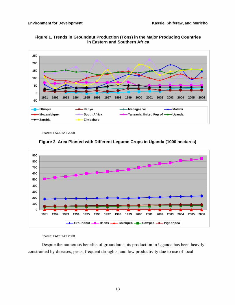
Uganda is one of the major producers of groundnuts in eastern and southern Africa (figure 1). Groundnuts are the second most widely grown legume in Uganda after the common bean (figure 2) and are a source of inexpensive protein and cash income for the rural poor and smallholder farmers. In addition, it increases soil productivity by returning atmospheric nitrogen to the soil (Coelli and Fleming 2004). In many communities where the crop is grown, its leaves and haulms (stems) make nutritious animal feed, while the groundnut meal (a byproduct of oil extraction) is another important source of livestock feed.

9 Namely, Teso, Lango, banana-cotton-millet, and montane—four of Uganda’s seven climate and agro-ecological zones (Mwebaze 1999).


13

Figure 1. Trends in Groundnut Production (Tons) in the Major Producing Countries in Eastern and Southern Africa

-50

0

50

100

150

200

250

1991 1992 1993 1994 1995 1996 1997 1998 1999 2000 2001 2002 2003 2004 2005 2006

Ethiopia Kenya Madagascar MalawiMozambique South Africa Tanzania, United Rep of UgandaZambia Zimbabwe

Source: FAOSTAT 2008

Figure 2. Area Planted with Different Legume Crops in Uganda (1000 hectares)

0

100

200

300

400

500

600

700

800

900

1991 1992 1993 1994 1995 1996 1997 1998 1999 2000 2001 2002 2003 2004 2005 2006

Groundnut Beans Chickpea Cowpea Pigeonpea

Source: FAOSTAT 2008

Despite the numerous benefits of groundnuts, its production in Uganda has been heavily constrained by diseases, pests, frequent droughts, and low productivity due to use of local


14

varieties. Bonabana-Wabbi et al. (2006), for instance, noted that groundnut losses in Uganda from pests and diseases generally exceeded those from soil infertility, drought, and poor planting material. At the same time, rosette disease10 has been a major challenge to productivity enhancement. In response to these constraints, NARO in collaboration with ICRISAT used ICRISAT’s improved groundnut materials to start a targeted research program in the early 1990s that specifically addressed these challenges. A total of five improved groundnut varieties were released by the end of 2002 as a result.

Descriptive statistics of adoption status for several of the variables used in the analysis are presented in table 1. The dataset contains 945 farm households, but after removing missing observations for some variables, we had 927 observations. About 59% and 41% of sampled households were improved groundnut and local groundnut adopters, respectively. The survey collected extensive information on several factors, including household characteristics and asset endowments, varieties of groundnuts, area planted, costs of production, crop production, indicators of access to infrastructure, market participation, household food security, household membership in different rural institutions, and household income sources.

The percentage of sample households who assessed themselves as food self-sufficient was about 83% (86.8% and 84.3% for adopters and non-adopters, respectively). About 86% and 51.6% of sample households participated in both crop selling and buying activities, respectively. On average about 90.7% (50.9%) and 82.6% (66.95%) of adopters and non-adopters participated in crop selling (buying) activities, respectively. The sample households seem to be relatively well connected to markets because the average walking distance from residences to markets (village and main market) and all weather roads was less than or equal to 6 km (table 1).

Adopters of groundnut technology seemed to be better off than non-adopters. Average annual total household income per capita was UGX 522,284 (US$ 282) and UGX 476,148 ($257)11 for adopters and non-adopters, respectively. There was a high correlation (67%) between crop income and total household income. These findings suggest that agricultural technology might have a role in improving household well being, but—given that adoption is endogenous—a simple comparison of the income of adopters and non-adopters has no causal interpretation. That is, this income difference may not be the result of groundnut technology

10 A viral disease transmitted by aphids. 11 The official exchange rate averaged about UGX 1,846 per US$ 1 in 2006.


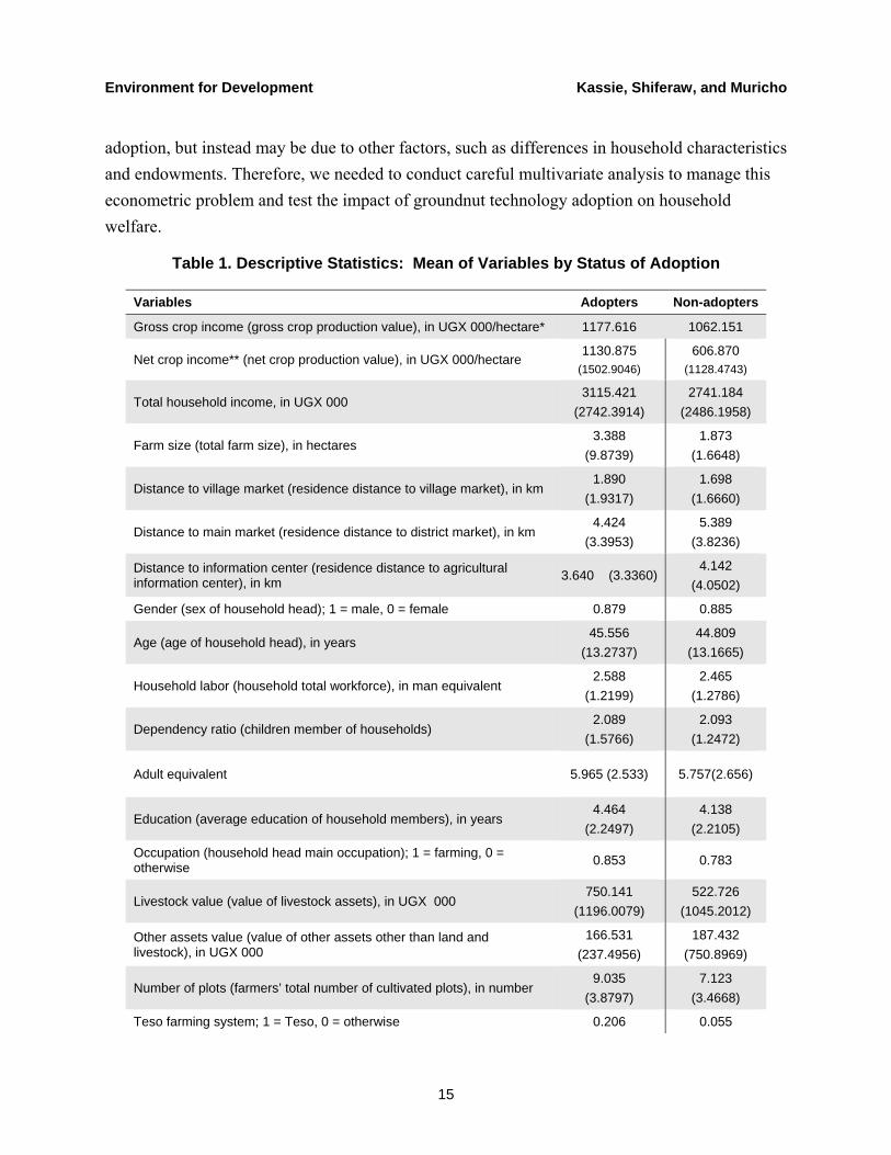
15

adoption, but instead may be due to other factors, such as differences in household characteristics and endowments. Therefore, we needed to conduct careful multivariate analysis to manage this econometric problem and test the impact of groundnut technology adoption on household welfare.

Table 1. Descriptive Statistics: Mean of Variables by Status of Adoption

Variables Adopters Non-adopters

Gross crop income (gross crop production value), in UGX 000/hectare* 1177.616 1062.151

Net crop income** (net crop production value), in UGX 000/hectare 1130.875

(1502.9046) 606.870

(1128.4743)

Total household income, in UGX 000 3115.421

(2742.3914) 2741.184

(2486.1958)

Farm size (total farm size), in hectares 3.388

(9.8739) 1.873

(1.6648)

Distance to village market (residence distance to village market), in km 1.890

(1.9317) 1.698

(1.6660)

Distance to main market (residence distance to district market), in km 4.424

(3.3953) 5.389

(3.8236)

Distance to information center (residence distance to agricultural information center), in km 3.640 (3.3360)

4.142 (4.0502)

Gender (sex of household head); 1 = male, 0 = female 0.879 0.885

Age (age of household head), in years 45.556

(13.2737) 44.809

(13.1665)

Household labor (household total workforce), in man equivalent 2.588

(1.2199) 2.465

(1.2786)

Dependency ratio (children member of households) 2.089

(1.5766) 2.093

(1.2472)

Adult equivalent 5.965 (2.533) 5.757(2.656)

Education (average education of household members), in years 4.464

(2.2497) 4.138

(2.2105)

Occupation (household head main occupation); 1 = farming, 0 = otherwise 0.853 0.783

Livestock value (value of livestock assets), in UGX 000 750.141

(1196.0079) 522.726

(1045.2012)

Other assets value (value of other assets other than land and livestock), in UGX 000

166.531 (237.4956)

187.432 (750.8969)

Number of plots (farmers’ total number of cultivated plots), in number 9.035

(3.8797) 7.123

(3.4668)

Teso farming system; 1 = Teso, 0 = otherwise 0.206 0.055


16

Lango farming system; 1 = Lango, 0 = otherwise 0.154 0.126

Banana-cotton-millet (BCM) farming system; 1 = BCM, 0 = otherwise 0.429

(0.4978) 0.429

(0.4998)

Montane farming system; 1 = montane, 0 = otherwise 0.110 0.188

West Nile farming system; 1 = West Nile, 0 = otherwise 0.101 0.202

Farmers organization; 1 = member, 0 = non-member 0.708 0.526

Participation in off-farm activity; 1 = yes, 0 = otherwise 0.725 0.888

Number of observations 545 382

Note: Standard deviation is in parentheses. * UGX = Uganda shilling. The official exchange rate averaged about UGX 1,846 per US$ 1 in 2006. ** Costs for fertilizer, labor, seed, and animal power for plowing deducted from value of crop production.

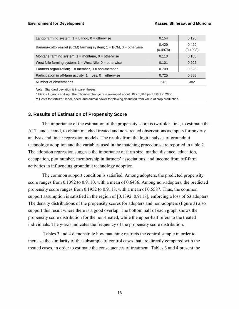
3. Results of Estimation of Propensity Score

The importance of the estimation of the propensity score is twofold: first, to estimate the ATT; and second, to obtain matched treated and non-treated observations as inputs for poverty analysis and linear regression models. The results from the logit analysis of groundnut technology adoption and the variables used in the matching procedures are reported in table 2. The adoption regression suggests the importance of farm size, market distance, education, occupation, plot number, membership in farmers’ associations, and income from off-farm activities in influencing groundnut technology adoption.

The common support condition is satisfied. Among adopters, the predicted propensity score ranges from 0.1392 to 0.9110, with a mean of 0.6436. Among non-adopters, the predicted propensity score ranges from 0.1952 to 0.9118, with a mean of 0.5587. Thus, the common support assumption is satisfied in the region of [0.1392, 0.9118], enforcing a loss of 63 adopters. The density distributions of the propensity scores for adopters and non-adopters (figure 3) also support this result where there is a good overlap. The bottom half of each graph shows the propensity score distribution for the non-treated, while the upper-half refers to the treated individuals. The y-axis indicates the frequency of the propensity score distribution.

Tables 3 and 4 demonstrate how matching restricts the control sample in order to increase the similarity of the subsample of control cases that are directly compared with the treated cases, in order to estimate the consequences of treatment. Tables 3 and 4 present the


17

balancing information for propensity scores and for each covariate before and after matching.12 We used the standardized bias difference between treatment and control samples as a convenient way to quantify the bias between treatment and control samples. In almost all cases, it is evident that sample differences in the raw data (unmatched data) significantly exceed those in the samples of matched cases. The process of matching thus creates a high degree of covariate balance between the treatment and control samples that are used in the estimation procedure.

Table 2. Estimation of Propensity Score: Logit Model (Dependent Variable: Adoption [0/1])

Variables Estimates Variables Estimates

Ln(farm size) 0.2172** (0.0919)

Livestock value -0.0000 (0.0001)

Distance to village market -0.0197 (0.0461)

Ln(other asset value) 0.0953

(0.0689)

Distance to main market -0.1071 (0.1098)

Number of plots 0.1490*** (0.0237)

Distance to information center

-0.0358 (0.0244)

Farmers association 1.0045*** (0.1671)

Gender 0.0181

(0.2536) Participation in off-farm activity

Age 0.0090

(0.0064) Teso farming system

2.6124*** (0.3491)

Household labor -0.1306* (0.0720)

Lango farming system 0.7191** (0.3282)

Dependency ratio -0.0232 (0.0639)

Banana-cotton-millet system 0.5180** (0.2522)

Education 0.0773* (0.0431)

Montane farming system -0.0354 (0.3033)

Occupation 0.5170** (0.2167) Constant

-2.7363*** (0.6312)

Summary Statistics

- Pseudo R-squared 0.18

- LR chi-square 175.06***

12 The common support density distribution figures and covariate balancing tests results are obtained using the Stata 10 pstest command (Leuven and Sianesi 2003).


18

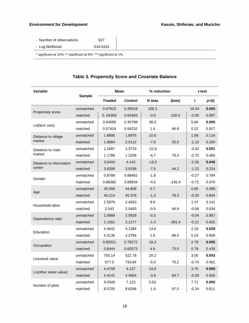
- Number of observations 927

- Log likelihood -516.6161

* significant at 10%; ** significant at 5%; *** significant at 1%.

Table 3. Propensity Score and Covariate Balance

Variable Sample

Mean % reduction t-test

Treated Control % bias |bias| t p>|t|

Propensity score unmatched 0.67815 0.45919 106.3 16.04 0.000

matched 0. 64359 0.64363 -0.0 100.0 -0.00 0.997

Ln(farm size) unmatched 0.64558 0.30788 38.3 5.66 0.000

matched 0.57424 0.56232 1.4 96.8 0.22 0.827

Distance to village market

unmatched 1.8895 1.6975 10.6 1.58 0.116

matched 1.8684 2.0112 -7.9 25.6 -1.13 0.260

Distance to main market

unmatched 1.1687 1.3733 -22.8 -3.43 0.001

matched 1.1786 1.2208 -4.7 79.4 -0.70 0.483

Distance to information center

unmatched 3.6404 4.142 -13.5 -2.06 0.040

matched 3.6399 3.9196 -7.5 44.2 -1.22 0.224

Gender unmatched 0.8789 0.88482 -1.8 -0.27 0.784

matched 0.88382 0.89834 -4.5 -145.4 -0.72 0.470

Age unmatched 45.556 44.809 5.7 0.85 0.398

matched 45.214 45.376 -1.2 78.3 -0.20 0.844

Household labor unmatched 2.5876 2.4653 9.8 1.47 0.141

matched 2.543 2.5493 -0.5 94.9 -0.08 0.934

Dependency ratio unmatched 2.0889 2.0928 -0.3 -0.04 0.967

matched 2.1081 2.1277 -1.4 -391.4 -0.21 0.832

Education unmatched 4.4642 4.1384 14.6 2.19 0.029

matched 4.4136 4.3794 1.5 89.5 0.24 0.808

Occupation unmatched 0.85321 0.78272 18.3 2.78 0.005

matched 0.8444 0.82573 4.9 73.5 0.78 0.435

Livestock value unmatched 750.14 522.78 20.2 3.00 0.003

matched 677.5 733.84 -5.0 75.2 -0.74 0.461

Ln(other asset value) unmatched 4.4709 4.137 24.8 3.76 0.000

matched 4.4142 4.4654 -3.8 84.7 -0.59 0.556

Number of plots unmatched 9.0349 7.123 0.52 7.71 0.000

matched 8.5705 8.6286 -1.6 97.0 -0.24 0.811


19

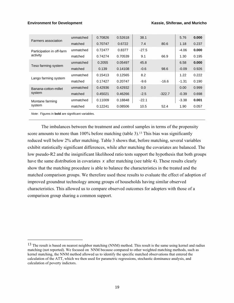
Farmers association unmatched 0.70826 0.52618 38.1 5.76 0.000

matched 0.70747 0.6722 7.4 80.6 1.18 0.237

Participation in off-farm activity

unmatched 0.72477 0.8377 -27.5 -4.06 0.000

matched 0.74274 0.70539 9.1 66.9 1.30 0.195

Teso farming system unmatched 0.2055 0.05497 45.8 6.58 0.000

matched 0.139 0.14108 -0.6 98.6 -0.09 0.926

Lango farming system unmatched 0.15413 0.12565 8.2 1.22 0.222

matched 0.17427 0.20747 -9.6 -16.6 -1.31 0.190

Banana-cotton-millet system

unmatched 0.42936 0.42932 0.0 0.00 0.999

matched 0.45021 0.46266 -2.5 -322.7 -0.39 0.698

Montane farming system

unmatched 0.11009 0.18848 -22.1 -3.38 0.001

matched 0.12241 0.08506 10.5 52.4 1.90 0.057

Note: Figures in bold are significant variables.

The imbalances between the treatment and control samples in terms of the propensity score amounts to more than 100% before matching (table 3).13 This bias was significantly reduced well below 2% after matching. Table 3 shows that, before matching, several variables exhibit statistically significant differences, while after matching the covariates are balanced. The low pseudo-R2 and the insignificant likelihood ratio tests support the hypothesis that both groups have the same distribution in covariates x after matching (see table 4). These results clearly show that the matching procedure is able to balance the characteristics in the treated and the matched comparison groups. We therefore used these results to evaluate the effect of adoption of improved groundnut technology among groups of households having similar observed characteristics. This allowed us to compare observed outcomes for adopters with those of a comparison group sharing a common support.

13 The result is based on nearest neighbor matching (NNM) method. This result is the same using kernel and radius matching (not reported). We focused on NNM because compared to other weighted matching methods, such as kernel matching, the NNM method allowed us to identify the specific matched observations that entered the calculation of the ATT, which we then used for parametric regressions, stochastic dominance analysis, and calculation of poverty indictors.


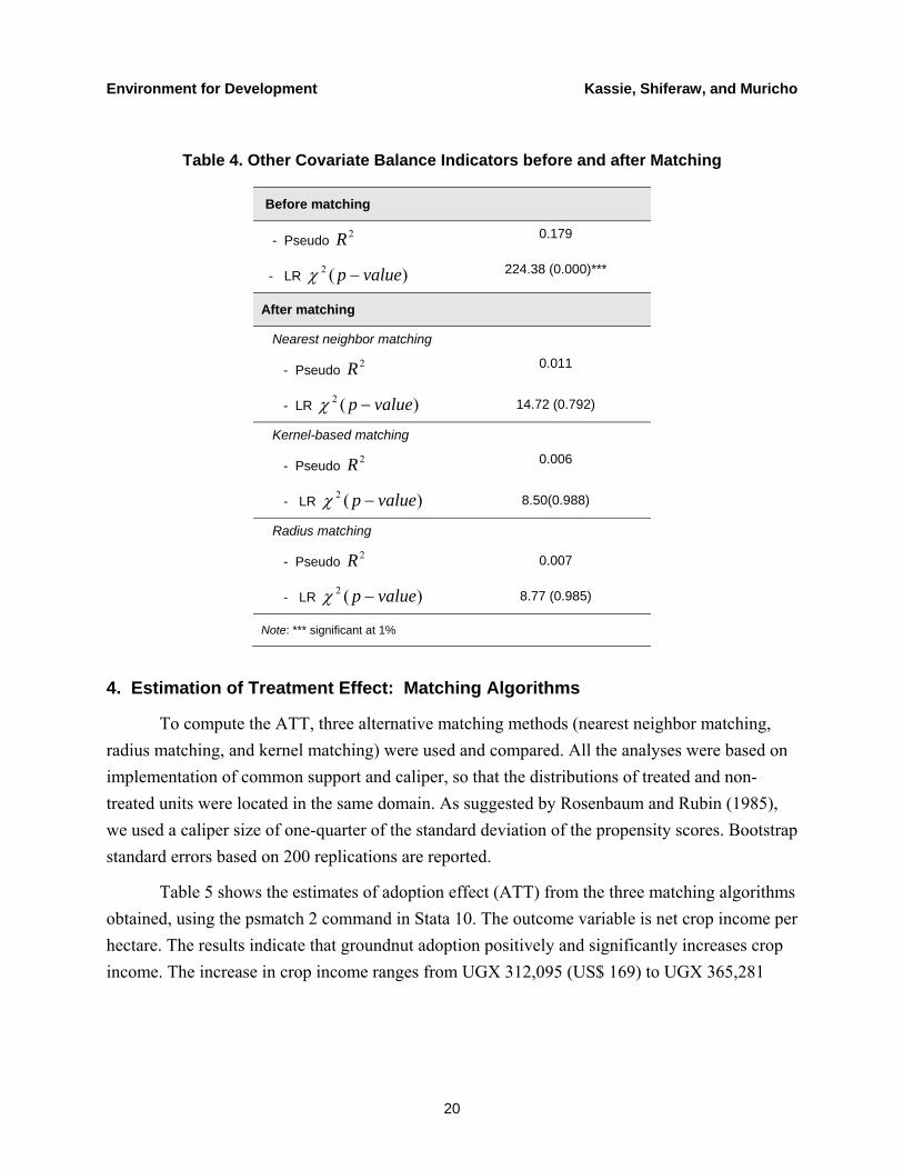
20

Table 4. Other Covariate Balance Indicators before and after Matching

Before matching

- Pseudo 2R 0.179

- LR )(2 valuep −χ 224.38 (0.000)***

After matching

Nearest neighbor matching

- Pseudo 2R 0.011

- LR )(2 valuep −χ 14.72 (0.792)

Kernel-based matching

- Pseudo 2R 0.006

- LR )(2 valuep −χ 8.50(0.988)

Radius matching

- Pseudo 2R 0.007

- LR )(2 valuep −χ 8.77 (0.985)

Note: *** significant at 1%

4. Estimation of Treatment Effect: Matching Algorithms

To compute the ATT, three alternative matching methods (nearest neighbor matching, radius matching, and kernel matching) were used and compared. All the analyses were based on implementation of common support and caliper, so that the distributions of treated and non-treated units were located in the same domain. As suggested by Rosenbaum and Rubin (1985), we used a caliper size of one-quarter of the standard deviation of the propensity scores. Bootstrap standard errors based on 200 replications are reported.

Table 5 shows the estimates of adoption effect (ATT) from the three matching algorithms obtained, using the psmatch 2 command in Stata 10. The outcome variable is net crop income per hectare. The results indicate that groundnut adoption positively and significantly increases crop income. The increase in crop income ranges from UGX 312,095 (US$ 169) to UGX 365,281


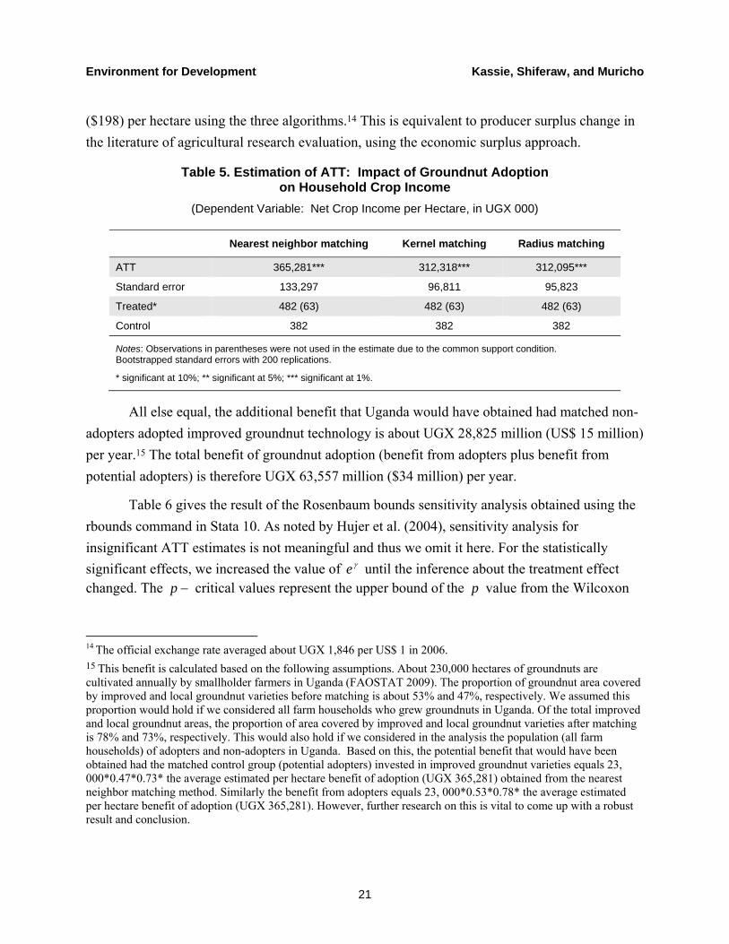
21

($198) per hectare using the three algorithms.14 This is equivalent to producer surplus change in the literature of agricultural research evaluation, using the economic surplus approach.

Table 5. Estimation of ATT: Impact of Groundnut Adoption on Household Crop Income

(Dependent Variable: Net Crop Income per Hectare, in UGX 000)

Nearest neighbor matching Kernel matching Radius matching

ATT 365,281*** 312,318*** 312,095***

Standard error 133,297 96,811 95,823

Treated* 482 (63) 482 (63) 482 (63)

Control 382 382 382

Notes: Observations in parentheses were not used in the estimate due to the common support condition. Bootstrapped standard errors with 200 replications.

* significant at 10%; ** significant at 5%; *** significant at 1%.

All else equal, the additional benefit that Uganda would have obtained had matched non-adopters adopted improved groundnut technology is about UGX 28,825 million (US$ 15 million) per year.15 The total benefit of groundnut adoption (benefit from adopters plus benefit from potential adopters) is therefore UGX 63,557 million ($34 million) per year.

Table 6 gives the result of the Rosenbaum bounds sensitivity analysis obtained using the rbounds command in Stata 10. As noted by Hujer et al. (2004), sensitivity analysis for insignificant ATT estimates is not meaningful and thus we omit it here. For the statistically significant effects, we increased the value of γe until the inference about the treatment effect changed. The −p critical values represent the upper bound of the p value from the Wilcoxon

14 The official exchange rate averaged about UGX 1,846 per US$ 1 in 2006. 15 This benefit is calculated based on the following assumptions. About 230,000 hectares of groundnuts are cultivated annually by smallholder farmers in Uganda (FAOSTAT 2009). The proportion of groundnut area covered by improved and local groundnut varieties before matching is about 53% and 47%, respectively. We assumed this proportion would hold if we considered all farm households who grew groundnuts in Uganda. Of the total improved and local groundnut areas, the proportion of area covered by improved and local groundnut varieties after matching is 78% and 73%, respectively. This would also hold if we considered in the analysis the population (all farm households) of adopters and non-adopters in Uganda. Based on this, the potential benefit that would have been obtained had the matched control group (potential adopters) invested in improved groundnut varieties equals 23, 000*0.47*0.73* the average estimated per hectare benefit of adoption (UGX 365,281) obtained from the nearest neighbor matching method. Similarly the benefit from adopters equals 23, 000*0.53*0.78* the average estimated per hectare benefit of adoption (UGX 365,281). However, further research on this is vital to come up with a robust result and conclusion.


22

signed rank test for estimated adoption effect (ATT) for each level of unobserved selection bias ( γe ). Given that the estimated treatment effect is positive, the lower bounds under the assumption that the true treatment effect has been underestimated were less interesting (Becker and Caliendo 2007) and therefore not reported in this paper.

Table 6 shows that the null hypothesis of no effect of groundnut technology adoption on crop income is not plausible. The positive effect of adoption is not sensitive to selection bias due to unobserved variables, even if we allow adopters and non-adopters to differ by as much as 65% in terms of unobserved covariate. The critical value of γe , at which point we would have to

question our conclusion of a positive effect of groundnut technology adoption, starts from 7.1=γe . This is a large value since we included the most important variables that affect both the

adoption decision and the outcome variable. Moreover, as noted by Becker and Caliendo (2007), these sensitivity results are worst-case scenarios. That is, a critical value of 7.1=γe does not mean that unobserved heterogeneity exists and adoption of groundnut technology has no effect on the crop income. It only states that the confidence interval for the effect would include zero if an unobserved variable caused the odds ratio of adoption to differ between adopters and non-adopters groups by a factor of 1.7. Based on this result, we can conclude that the ATT estimates in table 3 are a pure effect of improved groundnut technology adoption.

Table 6. Rosenbaum Bound Sensitivity Analysis Test for Hidden Bias

γe criticalp −

1 0001.0<

1.10 0001.0<

1.20 0001.0<

1.30 0001.0

1.40 001.0

1.50 011.0

1.60 046.0

1.65 081.0 1.70 129.0

1.80 269.0

1.90 449.0

2.00 631.0


23

5. Estimation of Average Treatment Effect: Switching Regression Approach

Table 6 reports estimates of the switching regression results. The standard error is corrected for any form of arbitrary heteroskedasticity. The results in table 4 indicate that market-distance and farming-system variables influence net crop income per hectare. To calculate the ATT from the switching regression approach, the difference in mean predicted net crop income values obtained by estimating equation (4) is taken into account. The switching regression result is in line with the propensity score matching estimates. The ATT, using the switching regression framework, is UGX 437,592 (US$ 237).

In sum, the above results underscore the importance of groundnut technology adoption in increasing crop income. This supports to examining the poverty reduction impact of groundnut technology adoption we shall discuss below.

6. Estimation of Groundnut Adoption Impact on Poverty Alleviation

The objective here was to test whether the level of poverty differs between adopters and non-adopters using Foster-Greer-Thorbecke poverty indices and stochastic dominance tests. Looking at the poverty indices (poverty headcount, poverty gap and poverty square gap) in table 7, it is apparent that the incidence of poverty, depth of poverty and severity of poverty are lower among the adopters than the non.-adopters. The stochastic dominance tests show a similar result.

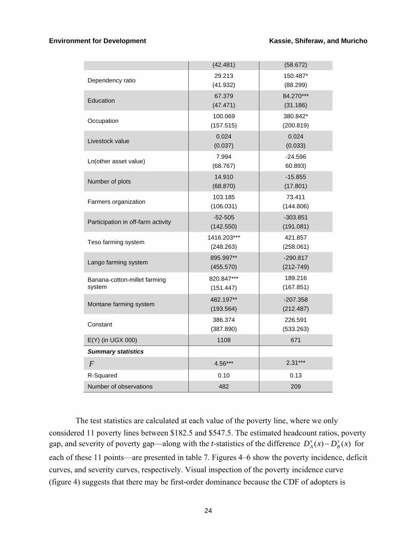
Table 7. Switching Regression Estimates (Dependent Variables: Net Crop Income per Hectare)

Variables Adopters Non-adopters

Estimates Estimates

Ln(farm size) -81.142 (95.316)

172.001 (127.204)

Distance to village market -28.857 (40.823)

-56.487** (24.630)

Distance to main market -175.459***

(62.101) -59.092 (79.494)

Distance to information center 19.958

(14.425) -16.739

()15.775)

Gender -545.727 (462.547)

240.941 (253.037)

Age 1.553

(3.577) -7.626* (4.406)

Household labor -27.595 43.119


24

(42.481) (58.672)

Dependency ratio 29.213

(41.932) 150.487* (88.299)

Education 67.379

(47.471) 84.270*** (31.186)

Occupation 100.069

(157.515) 380.842* (200.819)

Livestock value 0.024

(0.037) 0.024

(0.033)

Ln(other asset value) 7.994

(68.767) -24.596 60.893)

Number of plots 14.910

(68.870) -15.855 (17.801)

Farmers organization 103.185

(106.031) 73.411

(144.806)

Participation in off-farm activity -52-505

(142.550) -303.851 (191.081)

Teso farming system 1416.203*** (248.263)

421.857 (258.061)

Lango farming system 895.997** (455.570)

-290.817 (212-749)

Banana-cotton-millet farming system

820.847*** (151.447)

189.216 (167.851)

Montane farming system 482.197** (193.564)

-207.358 (212.487)

Constant 386.374

(387.890) 226.591

(533.263)

E(Y) (in UGX 000) 1108 671

Summary statistics

F 4.56*** 2.31***

R-Squared 0.10 0.13

Number of observations 482 209

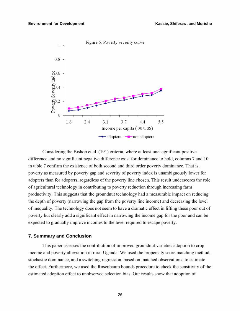
The test statistics are calculated at each value of the poverty line, where we only considered 11 poverty lines between $182.5 and $547.5. The estimated headcount ratios, poverty gap, and severity of poverty gap—along with the t-statistics of the difference )()( xDxD s

BsA − for

each of these 11 points—are presented in table 7. Figures 4–6 show the poverty incidence, deficit curves, and severity curves, respectively. Visual inspection of the poverty incidence curve (figure 4) suggests that there may be first-order dominance because the CDF of adopters is


25

always to the right of non-adopters but results of the test statistic for each value is insignificant indicating there is no first-order dominance. Given that first order dominance is not observed, we searched for higher order dominances (second and third order).


26

Considering the Bishop et al. (191) criteria, where at least one significant positive difference and no significant negative difference exist for dominance to hold, columns 7 and 10 in table 7 confirm the existence of both second and third order poverty dominance. That is, poverty as measured by poverty gap and severity of poverty index is unambiguously lower for adopters than for adopters, regardless of the poverty line chosen. This result underscores the role of agricultural technology in contributing to poverty reduction through increasing farm productivity. This suggests that the groundnut technology had a measurable impact on reducing the depth of poverty (narrowing the gap from the poverty line income) and decreasing the level of inequality. The technology does not seem to have a dramatic effect in lifting these poor out of poverty but clearly add a significant effect in narrowing the income gap for the poor and can be expected to gradually improve incomes to the level required to escape poverty.

7. Summary and Conclusion

This paper assesses the contribution of improved groundnut varieties adoption to crop income and poverty alleviation in rural Uganda. We used the propensity score matching method, stochastic dominance, and a switching regression, based on matched observations, to estimate the effect. Furthermore, we used the Rosenbaum bounds procedure to check the sensitivity of the estimated adoption effect to unobserved selection bias. Our results show that adoption of


27

improved groundnut varieties is associated with increased crop income and contributed to moving farm households out of poverty. The results are insensitive to unobserved selection bias. This suggests that developing and promoting appropriate agricultural technologies can contribute to the achievements of the Millennium Development Goal of eradicating poverty and hunger in the developing countries.


28

References

Alwang, J., and Siegel, B.P. 2003. Measuring the Impacts of Agricultural Research on Poverty Reduction. Agricultural Economics 29:1–14.

Andreas, C., A.C. Drichoutis, P. Lazaridis, and R.M. Nayga Jr. 2009. Can Mediterranean Diet Really Influence Obesity? Evidence from Propensity Score Matching. European Journal of Health Economics 10: 371–88.

Becker, S.O., and M. Caliendo. 2007. Sensitivity Analysis for Average Treatment Effects. Stata Journal 7(1): 71–83.

Bishop, J.A., J.P. Formby, and P.D. Thistle. 1989. Statistical Inference, Income Distributions, and Social Welfare. In Research on Economic Inequality, vol. 1, edited by D.J. Slottje. Greenwich, CT, USA: JAI Press, 49–82.

Bonabana-Wabbi, J., D.B. Taylor, and V. Kasenge. 2006. A Limited Dependent Variable Analysis of Integrated Pest Management Adoption in Uganda. Paper presented at the American Agricultural Economics Association Annual Meeting, Long Beach, CA, USA, July 23–26, 2006.

Bryon, A., R. Dorsett, and S. Purdon. 2000. The Use of Propensity Score Matching in the Evaluation of Active Labour Market Policies. Working Paper, no. 4. London: Department of Work and Pensions. http://eprints.lse.ac.uk/4993/1/The_use_of_propensity_score_matching_in_the_evaluation_of_active_labour_market_policies.pdf. Accessed April 2010.

Caleindo, M., and S. Kopeinig. 2005. Some Practical Guidance for the Implementation of Propensity Score Matching. IZA Discussion Paper, no. 1588. Bonn, Germany: IZA. http://repec.iza.org/dp1588.pdf. Accessed April 2010.

Coelli, T., and E. Fleming. 2004. Diversification Economies and Specialization Efficiencies in a Mixed Food and Coffee Smallholder Farming System in Papua New Guinea. Agricultural Economics 31(2–3): 229–39.

de Janvry, A., and E. Sadoulet. 2001. World Poverty and the Role of Agricultural Technology: Direct and Indirect Effects. Journal of Development Studies 38(4): 1–26.

Dehejia, H.R., and S. Wahba. 2002. Propensity Score Matching Methods for Non-Experimental Causal Studies. Review of .Economic Statistics 84(1): 151–61.


29

Diprete, T., and M. Gangl. 2004. Assessing Bias in the Estimation of Causal Effects: Rosenbaum Bounds on Matching Estimators and Instrumental Variables Estimation with Imperfect Instruments. Sociological Methodology 34: 271–310.

ECA (Economic Commission for Africa). 2007. Economic Report on Africa 2007: Accelerating Africa’s Development through Diversification. Addis Ababa, Ethiopia: ECA.

FAOSTAT (Food and Agriculture Organization of the United Nations). 2009. FAOSTAT database. http://faostat.fao.org. Accessed April 2010.

———. 2008. FAOSTAT database. http://faostat.fao.org. Accessed April 2010.

Foster, J., J. Greer, and E. Thorbecke. 1984. A Class of Decomposable Poverty Measures. Econometrica 52: 761–66.

Heckman, J., H. Ichimura, J. Smith, and P. Todd. 1997. Matching as an Econometric Evaluation Estimator: Evidence from Evaluating a Job Training Programme. Review of Economics Studies 64: 605–654.

———.1998. Characterizing Selection Bias Using Experimental Data. Econometrica 66(5): 1017–1098.

Mendola, M. 2007. Agricultural Technology Adoption and Poverty Reduction: A Propensity-Score Matching Analysis for Rural Bangladesh. Food Policy 32: 372–93.

Moyo, S., G.W. Norton, J. Alwang, I. Rhinehart, and M.C. Demo. 2007. Peanut Research and Poverty Reduction: Impacts of Variety Improvement to Control Peanut Viruses in Uganda. American Journal of Agricultural Economics 89(2): 448–60.

Mwebaze, S.M.N. 1999. Country Pasture/Forage Resource Profiles: Uganda. Entebbe, Uganda: Department of Animal Production and Marketing, Ministry of Agriculture, Animal Industry, and Fisheries. http://www.fao.org/ag/AGP/AGPC/doc/counprof/Uganda/uganda.htm#3.%20CLIMATE%20AND%20AGROECOLOGICAL. Accessed April 2010.

Pinstrup-Andersen, P., and R. Pandya-Lorch. 1995. Agricultural Growth is the Key to Poverty Alleviation in Low Income Developing Countries. 2020 Brief. Washington, DC: International Food Policy Research Institute.

Ravallion, M. 1994. Is Poverty Increasing in the Developing World? Review of Income and Wealth Series 40(4): 359–76.


30

Rahman, S. 1999. Impact of Technological Change on Income Distribution and Poverty in Bangladesh Agriculture: An Empirical Analysis. Journal of International Development 11: 935–55.

Rosenbaum, P.R. 2002. Observational Studies. New York: Springer.

Rosenbaum, P.R., and D.B. Rubin. 1983. The Central Role of the Propensity Score in Observational Studies for Causal Effects. Biometrika 70(1): 41–55.

Smith, J., and P. Todd. 2005. Does Matching Overcome LaLonde’s Critique of Non-experimental Estimators? Journal of Econometrics 125(1-2): 305–353.

WHO (World Health Organization). 1985. Energy and Protein Requirements: Report of a Joint FAO/WHO/UNU Expert Consultation. World Health Organization Technical Report Series, no. 724. Geneva: WHO.

World Bank. 2007. World Development Report 2008: Agriculture for Development. Washington, DC: World Bank. http://siteresources.worldbank.org/INTWDR2008/Resources/WDR_00_book.pdf. Accessed 2010.

adoption and impact of improved groundnut varieties on ... · adoption and impact of improved...

Documents