the properties of jovian trojan asteroids listed in sdss...

Mon. Not. R. Astron. Soc. 377, 1393–1406 (2007) doi:10.1111/j.1365-2966.2007.11687.x

The properties of Jovian Trojan asteroids listed in SDSS Moving ObjectCatalogue 3

Gy. M. Szabo,1�† Z. Ivezic,2 M. Juric3 and R. Lupton3

1Department of Experimental Physics & Astronomical Observatory, University of Szeged, 6720 Szeged, Hungary2Department of Astronomy, University of Washington, Seattle, WA 98155, USA3Princeton University Observatory, Princeton, NJ 08544, USA

Accepted 2007 February 28. Received 2007 February 27; in original form 2007 January 18

ABSTRACTWe analyse 1187 observations of about 860 unique candidate Jovian Trojan asteroids listed inthe 3rd release of the Sloan Digital Sky Survey (SDSS) Moving Object Catalogue. The sampleis complete at the faint end to r = 21.2 mag (apparent brightness) and H = 13.8 (absolutebrightness, approximately corresponding to 10 km diameter). A subset of 297 detections ofpreviously known Trojans were used to design and optimize a selection method based onobserved angular velocity that resulted in the remaining objects. Using a sample of objectswith known orbits, we estimate that the candidate sample contamination is about 3 per cent.The well-controlled selection effects, the sample size, depth and accurate five-band UV–IR photometry enabled several new findings and the placement of older results on a firmerstatistical footing. We find that there are significantly more asteroids in the leading swarm (L4)than in the trailing swarm (L5): N(L4)/N(L5) = 1.6 ± 0.1, independently of limiting object’ssize. The overall counts normalization suggests that there are about as many Jovians Trojans asthere are main-belt asteroids down to the same size limit, in agreement with earlier estimates.We find that Trojan asteroids have a remarkably narrow colour distribution (root mean scatterof only ∼0.05 mag) that is significantly different from the colour distribution of the main-beltasteroids. The colour of Trojan asteroids is correlated with their orbital inclination, in a similarway for both swarms, but appears uncorrelated with the object’s size. We extrapolate the resultspresented here and estimate that the Large Synoptic Survey Telescope will determine orbits,accurate colours and measure light curves in six photometric bandpasses for about 100 000Jovian Trojan asteroids.

Key words: astronomical data bases: miscellaneous – catalogues – minor planets, asteroids– Solar system: general.

1 I N T RO D U C T I O N

Jovian Trojan asteroids are found in two swarms around the L4 andL5 Lagrangian points of Jupiter’s orbit (for a review see Marzariet al. 2001). The first Jovian Trojan was discovered a century agoby Max Wolf. Nearly 2000 Jovian Trojans were discovered by theend of 2003 (Bendjoya et al. 2004, hereafter B04). About half arenumbered asteroids with reliable orbits (Marzari et al. 2001). Theirtotal number is suspected to be similar to the number of the main-beltasteroids1 (Shoemaker, Shoemaker & Wolfe 1989).

�E-mail: [email protected]†Magyary Zoltan Postdoctoral Research Fellow.1 Recent work supports this claim. Ivezic et al. (2001) estimated that thenumber of main-belt asteroids with diameters larger than 1 km is 740 000,with a somewhat higher estimate by Tedesco, Cellino & Zappala (2005), andJewitt, Trujillo & Luu (2000) estimated that there are between 520 000 and790 000 Jovian Trojans above the same size limit.

The Trojans’ positions relative to Jupiter librate around L4 (lead-ing swarm) and L5 (trailing swarm) with periods of the order of ahundred years. Their orbital eccentricity is typically smaller (<0.2)than those of main-belt asteroids, but the inclinations are compara-ble, with a few known Trojans (KTs) having inclinations larger than30◦. The largest objects have diameters exceeding 100 km. Theytypically have featureless (D-type) spectra and extremely low op-tical albedo (Tedesco 1989; Fernandez, Sheppard & Jewitt 2003).These spectral properties are similar to those of cometary nuclei.However, there are also Trojans that have P or common C-type clas-sification, mostly found in the trailing swarm (Fitzsimmons et al.1994). The collisional grinding of Trojan asteroids is supported bytheir observed size distribution (Jewitt, Trujillo & Luu 2000, here-after JTL).

Numerous studies of the origin of Jovian Trojans are based ontwo different hypothesis. According to one of them, the Jovian Tro-jans were formed simultaneously with Jupiter in the early phaseof the solar nebula. The growing Jupiter could have captured and

C© 2007 The Authors. Journal compilation C© 2007 RAS

1394 G. M. Szabo et al.

stabilized the plantesimals near its L4 and L5 points (Peale 1993).The other hypothesis assumes that the majority of Jovian Trojanswere captured over a much longer period, and were formed eitherclose to Jupiter, or were gravitationally scattered from the main beltor elsewhere in the Solar System (Jewitt 1996). The spectral comet-like appearance of many Trojans is consistent with the scatteringfrom the outer Solar System.

Depending on the importance of gas drag when Trojans formed,the L4 and L5 swarms could have different dynamics. The presenceof significant gas drag helps stabilize orbits around the L5 point. Onthe other hand, these trailing objects have later evolution differentfrom the leading swarm because planetary migration destabilizesL5 (Gomes 1998). Morbidelli et al. (2005) recently suggested amore complex picture: the present permanent Trojan populationsare built up by objects that were trapped after the 1:2 mean motionresonance crossing of the Saturn and the Jupiter. Therefore, it ispossible that size distributions, or detailed distributions of orbitalparameters, could be different for the leading and trailing swarm.However, no such differences have yet been found (Marzari et al.2001, and references therein).

It is noteworthy that there are severe observational biases in thesample of known Jovian Trojans due to their large distance. For ex-ample, although the numbers of main-belt asteroids and Trojans toa given size limit are similar, only about 1 per cent of the known ob-jects belong to the latter group. This is a consequence of the fact thata Trojan at a heliocentric distance of 5.2 au is about 4 mag fainterthan a same-size main-belt asteroid at a heliocentric distance of2.5 au (as observed in opposition, and not accounting for differ-ences in albedo, which further diminishes the Trojan’s apparentmagnitude).

Here we present an analysis of the properties of about 1000 knownand candidate Jovian Trojan asteroids based on the data collected bySloan Digital Sky Survey (SDSS, York et al. 2000). SDSS, althoughprimarily designed for observations of extragalactic objects, is sig-nificantly contributing to studies of the Solar System objects becauseasteroids in the imaging survey must be explicitly detected and mea-sured to avoid contamination of the samples of extragalactic objectsselected for spectroscopy. Preliminary analysis of SDSS commis-sioning data (Ivezic et al. 2001, hereafter I01) showed that SDSSwill increase the number of asteroids with accurate five-colour pho-tometry by more than two orders of magnitude, and to a limit about5 mag fainter (7 mag when the completeness limits are compared)than previous multicolour surveys (e.g. The Eight Colour AsteroidSurvey, Zellner, Tholen & Tedesco 1985). As we demonstrate be-low, the SDSS data extend the faint completeness limit for Trojanasteroids by about 1.5 mag (to a limiting diameter of ∼10 km).

The large sample and accurate astrometric and five-band pho-tometric SDSS data to a much fainter limit than reached by mostprevious surveys, together with suitable ways to quantify selectioneffects, allow us to address the following questions.

(i) What is the size distribution of Jovian Trojans asteroids withdiameters larger than 10 km?

(ii) Do the leading and trailing swarms have the same size distri-bution (including both the distribution shape and the overall numberabove some size limit)?

(iii) What is their colour distribution in the SDSS photometricsystem, and how does it compare to the colour distribution of main-belt asteroids?

(iv) Is the colour distribution correlated with inclination, as sug-gested by a preliminary analysis of SDSS data (Ivezic et al. 2002a,hereafter I02a)?

(v) Are the Trojans’ size and colour correlated (as suggested byB04)?

(vi) Do the leading and trailing swarms have the same colourdistribution?

(vii) Is the size distribution correlated with inclination?

The SDSS asteroid data are described in Section 2, and in Sec-tion 3 we describe a novel method for selecting candidate JovianTrojan asteroids from SDSS data base. Analysis of the propertiesof selected objects, guided by the above questions, is presented inSection 4. We summarize our results in Section 5, and discuss theirimplications for the origin and evolution of Trojan asteroids.

2 S D S S O B S E RVAT I O N S O F M OV I N GO B J E C T S

SDSS is a digital photometric and spectroscopic survey using adedicated 2.5 m telescope at the Apache Point Observatory, whichwill cover 10 000 deg2 of the Celestial Sphere in the North Galacticcap, and a smaller (∼225 deg2) and deeper survey in the SouthernGalactic hemisphere (Abazajian et al. 2003, and references therein).The survey sky coverage will result in photometric measurementsfor over 108 stars and a similar number of galaxies. The flux densi-ties of detected objects are measured almost simultaneously (within∼5 min) in five bands (u, g, r, i and z) with effective wavelengthsof 3551, 4686, 6166, 7480 and 8932 Å (Fukugita et al. 1996; Gunnet al. 1998; Hogg et al. 2002; Smith et al. 2002). The photometriccatalogues are 95 per cent complete for point sources to limitingmagnitudes of 22.0, 22.2, 22.2, 21.3 and 20.5 in the North Galac-tic cap. Astrometric positions are accurate to about 0.1 arcsec percoordinate (rms) for sources brighter than 20.5m (Pier et al. 2003),and the morphological information from the images allows robuststar–galaxy separation (Lupton et al. 2001, 2002) to ∼21.5m. Thephotometric measurements are accurate to 0.02 mag (both absolutecalibration, and rms scatter for sources not limited by photon statis-tics; Ivezic et al. 2004). The recent fifth public Data Release (DR5)includes imaging data for ∼8000 deg2 of sky, and catalogues for2.15 × 108 objects. For more details please see Abazajian et al.(2003) and references therein.

SDSS Moving Object Catalogue2 (hereafter SDSS MOC) is apublic, value-added catalogue of SDSS asteroid observations (Ivezicet al. 2002b, hereafter I02b). It includes all unresolved objectsbrighter than r = 21.5 and with observed angular velocity in the0.05–0.5 deg d−1 interval. In addition to providing SDSS astromet-ric and photometric measurements, all observations are matched toknown objects listed in the ASTORB file (Bowell 2001), and to adata base of proper orbital elements (Milani 1999), as described indetail by Juric et al. (2002, hereafter J02). J02 determined that thecatalogue completeness (number of moving objects detected by thesoftware that are included in the catalogue, divided by the total num-ber of moving objects recorded in the images) is about 95 per cent,and its contamination rate is about 6 per cent (the number of entriesthat are not moving objects, but rather instrumental artefacts).

The third release of SDSS MOC used in this work contains mea-surements for over 204 000 asteroids. The quality of these data wasdiscussed in detail by I01, including a determination of the size andcolour distributions for main-belt asteroids. An analysis of correla-tion between colours and asteroid dynamical families was presentedby I02a. An interpretation of this correlation as the dependence ofcolour on family age (due to space weathering effect) was proposed

2 Available at http://www.sdss.org.

C© 2007 The Authors. Journal compilation C© 2007 RAS, MNRAS 377, 1393–1406

Jovian Trojan asteroids in SDSS MOC 3 1395

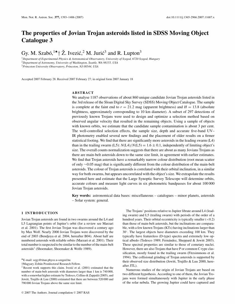
Figure 1. The dots show the osculating orbital inclination versus semimajoraxis distribution of 43 424 unique moving objects detected by the SDSS,and matched to objects with known orbital parameters listed in Bowell’sASTORB file (these data are publicly available in the third release of theSDSS Moving Object Catalogue. The dots are colour-coded according totheir colours measured by SDSS (see I02a for details, including analogousfigures constructed with proper orbital elements). Note that most main-beltasteroid families have distinctive colours. Jovian Trojans asteroids are foundat a ∼ 5.2 au, and display a correlation between the colour and orbitalinclination (objects with high inclination tend to be redder, see Section 4).

by Jedicke et al. (2004) and further discussed by Nesvorny et al.(2005). Multiple SDSS observations of objects with known orbitalparameters can be accurately linked, and thus SDSS MOC also con-tains rich information about asteroid colour variability, discussed indetail by Szabo et al. (2004).

The value of SDSS data becomes particularly evident when ex-ploring the correlation between colours and orbital parameters formain-belt asteroids. Fig. 1 uses a technique developed by I02a tovisualize this correlation. A striking feature of this figure is thecolour homogeneity and distinctiveness displayed by asteroid fam-ilies. This strong colour segregation provides firm support for thereality of asteroid dynamical families. Jovian Trojans asteroids arefound at a ∼ 5.2 au, and display a correlation between the colour andorbital inclination (objects with high inclination tend to be redder).On the other hand, the colour and orbital eccentricity (see Fig. 2)do not appear correlated.

The distribution of the positions of SDSS observing fields in acoordinate system centred on Jupiter and aligned with its orbit isshown in Fig. 3. As evident, both L4 and L5 regions are well coveredwith the available SDSS data. There are 313 unique known objects(from ASTORB file) in SDSS MOC whose orbital parameters areconsistent with Jovian Trojan asteroids (here defined as objects withsemimajor axis in the range 5.0–5.4 au). Since SDSS imaging depthis about 2 mag deeper than the completeness limit of ASTORBfile used to identify KTs, there are many more Trojan asteroids inSDSS MOC whose orbits are presently unconstrained. Nevertheless,they can be identified using a kinematic method described in thefollowing Section.

3 S E L E C T I O N O F T RO JA N A S T E RO I D S F RO MS D S S M OV I N G O B J E C T C ATA L O G U E

The angular velocity of moving objects measured by SDSS can beused as a proxy for their distance determination and classification

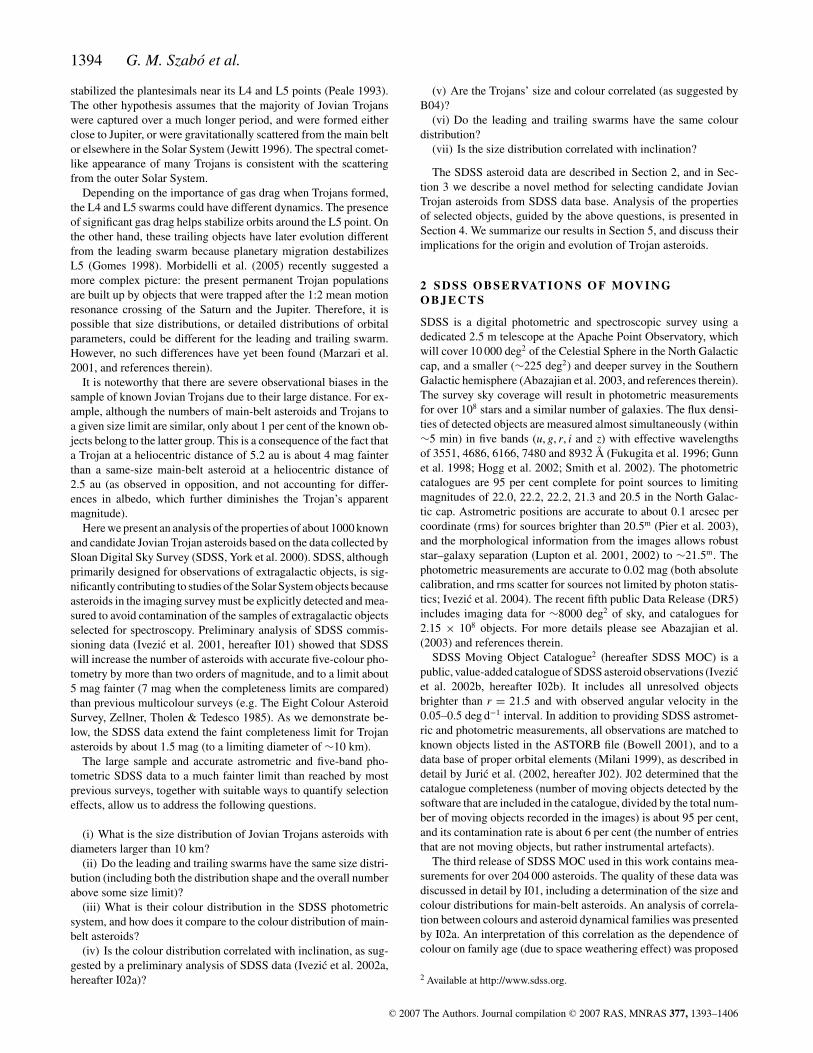
Figure 2. Analogous to Fig. 1, except that here the orbital eccentricity ver-sus semimajor axis distribution is shown. Note that there is no discerniblecorrelation between the colour and eccentricity for Jovian Trojan asteroids.

Figure 3. The distribution of the longitude of ∼440 000 9 × 13 arcmin2

large SDSS observing fields in a coordinate system centre on Jupiter andaligned with its orbit, as a function of observing epoch (green symbols).Fields obtained within 25◦ from the opposition are marked by black symbols.The two dashed lines mark the relative longitudes of the L4 (λJup = 60◦,leading swarm) and L5 (λJup = −60◦, trailing swarm) Lagrangian points.Both swarms are well sampled in the third release of SDSS Moving ObjectCatalogue.

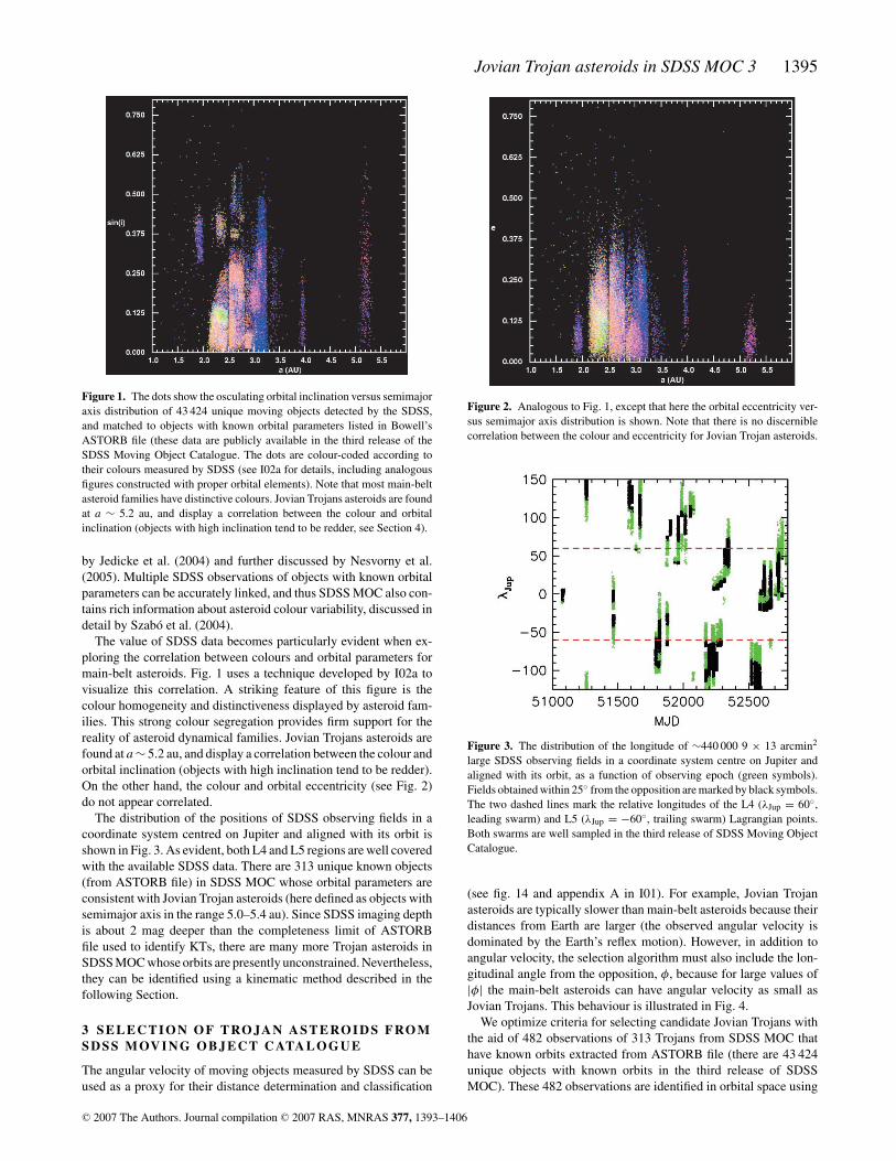
(see fig. 14 and appendix A in I01). For example, Jovian Trojanasteroids are typically slower than main-belt asteroids because theirdistances from Earth are larger (the observed angular velocity isdominated by the Earth’s reflex motion). However, in addition toangular velocity, the selection algorithm must also include the lon-gitudinal angle from the opposition, φ, because for large values of|φ| the main-belt asteroids can have angular velocity as small asJovian Trojans. This behaviour is illustrated in Fig. 4.

We optimize criteria for selecting candidate Jovian Trojans withthe aid of 482 observations of 313 Trojans from SDSS MOC thathave known orbits extracted from ASTORB file (there are 43 424unique objects with known orbits in the third release of SDSSMOC). These 482 observations are identified in orbital space using



Figure 4. The basis for the kinematic selection of CT asteroids from SDSSMoving Object Catalogue. The small dots in the top panel show the magni-tude of the measured angular velocity as a function of the longitudinal anglefrom the opposition for ∼43 000 unique objects with known orbits listedin the catalogue. The large dots show known Jovian Trojan asteroids. Thelines show adopted selection criteria for CTs (see text). The bottom panelis an analogous plot and shows the measured longitudinal component of theangular velocity (in ecliptic coordinate system) as a function of angle fromthe opposition. The CTs are selected in the three-dimensional v–vλ–φ space.

constraints 5.0 < a < 5.4 au and e < 0.2, and hereafter referred to asthe KTs. Of those, the majority (263) belong to the leading swarm.

We compare the angular velocity and φ distributions of theseobjects to those for the whole sample in Fig. 4. We find that thefollowing selection criteria result in a good compromise betweenthe selection completeness and contamination:

0.112 −(

φ

180

)2

< v < 0.155 −(

φ

128

)2

, (1)

−0.160 +(

φ

134

)2

< vλ < −0.125 +(

φ

180

)2

, (2)

for observations with −25 < φ < 25. That is, only observationsobtained relatively close to the opposition can be used to select asample with a low contamination rate by main-belt asteroids. Theadopted velocity limits are in good agreement with those proposedby JTL.

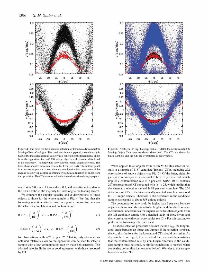
Figure 5. Analogous to Fig. 4, except that all ∼204 000 objects from SDSSMoving Object Catalogue are shown (blue dots). The CTs are shown byblack symbols, and the KTs are overplotted as red symbols.

When applied to all objects from SDSS MOC, this selection re-sults in a sample of 1187 candidate Trojans (CTs), including 272observations of known objects (see Fig. 5). Of the latter, eight ob-jects have semimajor axis too small to be a Trojan asteroid, whichimplies a contamination rate of 3 per cent. SDSS MOC contains297 observations of KTs obtained with |φ| < 25, which implies thatthe kinematic selection method is 89 per cent complete. The 264detections of KTs in the kinematically selected sample correspondto 191 unique objects. Therefore, 1187 detections in the candidatesample correspond to about 858 unique objects.

The contamination rate could be higher than 3 per cent becauseobjects with known orbits tend to be brighter and thus have smallermeasurement uncertainties for angular velocities than objects fromthe full candidate sample (for a detailed study of these errors andtheir correlation with other observables see I01). For this reason, weperform the following robustness test.

The above selection procedure does not include λJup, the longitu-dinal angle between an object and Jupiter. If the selection is robust,the λJup distributions for the known and CTs should be similar. Asdiscernible from Fig. 6, this is indeed the case and demonstratesthat the contamination rate by non-Trojan asteroids in the candi-date sample must be small. A similar conclusion is reached whencomparing colour distributions (see below). We refer to this samplehereafter as the CTs.



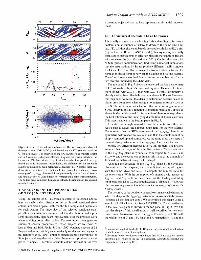
Figure 6. A test of the selection robustness. The top two panels show allthe objects from SDSS MOC (small blue dots), the KTs (red dots) and theCTs (black squares), as observed on the sky, in Jupiter’s coordinate systemand in φ versus λJup diagram. Although λJup was not used in selection, theknown and CTs have similar λJup distributions (the third panel from top,dotted and solid histograms, respectively), and different than for the wholesample, dominated by main-belt asteroids (dashed line). Note that these λJup

distributions are not corrected for the selection biases due to inhomogeneouscoverage of λJup–βJup plane (which are presumably similar for both knownand candidate objects), and thus are not representative of the true distribution.The bottom panel compares the angular velocity distributions of Trojans andmain-belt asteroids.

4 A NA LY S I S O F T H E P RO P E RT I E SO F T RO JA N A S T E RO I D S

Using the sample of CT asteroids selected as described above,here we analyse their distribution in the three-dimensional size–colour–inclination space, both for the full sample and separatelyfor each swarm. The large size of the selected candidate sam-ple allows accurate measurements of this distribution, and repre-sents an especially significant improvement over the previous workwhen studying colour distribution. The two largest homogeneousstudies of spectral properties of Jovian Trojans are by Jewitt &Luu (1990) and B04. Jewitt & Luu (1990) obtained spectra of 32Trojans and found that they are remarkably similar to cometary spec-tra. Bendjoya et al. (2004) obtained spectroscopic observations for34 objects and, together with older observations, produced a sam-ple of 73 objects. Therefore, accurate colour information for over

a thousand objects discussed here represents a substantial improve-ment.

4.1 The numbers of asteroids in L4 ad L5 swarms

It is usually assumed that the leading (L4) and trailing (L5) swarmscontain similar number of asteroids down to the same size limit(e.g. JTL). Although the number of known objects in L4 and L5 differ(e.g. as listed in Bowell’s ASTORB file), this asymmetry is usuallydismissed as due to complex selection biases in the sample of Trojanswith known orbits (e.g. Marzari et al. 2001). On the other hand, Pal& Suli (private communication) find using numerical simulationsthat the perturbations by Saturn produce different stability regionsfor L4 and L5. This effect is suspected to cause about a factor of 2population size difference between the leading and trailing swarms.Therefore, it seems worthwhile to examine the number ratio for thetwo swarms implied by the SDSS data.

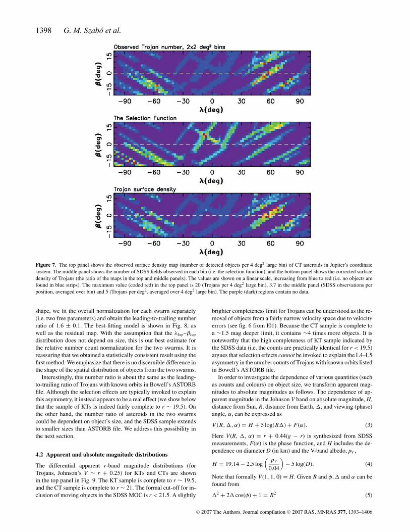
The top panel in Fig. 7 shows the observed surface density mapof CT asteroids in Jupiter’s coordinate system. There are 1.9 timesmore objects with λJup > 0 than with λJup < 0 (this asymmetry isalready easily discernible in histograms shown in Fig. 6). However,this map does not reveal true density distribution because selectionbiases are strong even when using a homogeneous survey such asSDSS. The most important selection effect is the varying number ofSDSS observations as a function of position relative to Jupiter, asshown in the middle panel.3 It is the ratio of these two maps that isthe best estimate of the underlying distribution of Trojan asteroids.This map is shown in the bottom panel in Fig. 7.

It is still not straightforward to use the counts from this cor-rected map to assess the number–count ratio for the two swarms.The reason is that the SDSS coverage of the λJup–βJup plane is notsymmetric with respect to λJup = 0, and thus the counts cannot besimply summed up and compared. At the same time, the shape ofthe underlying distribution in the λJup–βJup plane is not known.

We use two different methods to solve this problem. The first oneassumes that the shape of the true distribution of Trojan asteroidsin the λJup–βJup plane is symmetric with respect to λJup = 0 andβJup = 0, and the second one estimates this shape using a sample ofKTs and normalizes it using the CT sample.

Although the coverage of the λJup–βJup plane by the availableobservations is fairly sparse, there is sufficient overlap of regionswith the same |βJup| and |λJup| to compute the number ratio forthe two swarms. With the assumption of symmetry with respect toλJup = 0 and βJup = 0, we determine that the leading-to-trailingnumber ratio is 1.8 ± 0.2 (weighted average of all pixels). It appearsthat the leading swarm has almost twice as many objects as thetrailing swarm.

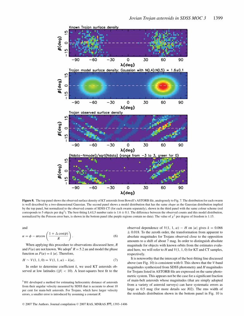
The accuracy of the number–count ratio estimate can be increasedwhen the shape of the λJup–βJup distribution is assumed to be known(because all the data are used). We determined this shape using asample of 1178 KT asteroids from ASTORB file. Their distributionin the λJup–βJup plane is shown in the top panel in Fig. 8. We findthat the shape of this distribution is well described by two two-dimensional Gaussians centred on βJup = 0◦ and λJup = ±60◦, withthe widths (σ ) of 9◦ and 14◦, for β and λ, respectively.4 Using this

3 Here we assume that the depth of SDSS imaging is constant, which is trueto within several tenths of a magnitude.4 The errors for these estimates are not larger than ∼0.5 and indicate that thedistribution of Trojans on the sky is not circularly symmetric around L4 andL5 points, as assumed by JTL.



Figure 7. The top panel shows the observed surface density map (number of detected objects per 4 deg2 large bin) of CT asteroids in Jupiter’s coordinatesystem. The middle panel shows the number of SDSS fields observed in each bin (i.e. the selection function), and the bottom panel shows the corrected surfacedensity of Trojans (the ratio of the maps in the top and middle panels). The values are shown on a linear scale, increasing from blue to red (i.e. no objects arefound in blue strips). The maximum value (coded red) in the top panel is 20 (Trojans per 4 deg2 large bin), 3.7 in the middle panel (SDSS observations perposition, averaged over bin) and 5 (Trojans per deg2, averaged over 4 deg2 large bin). The purple (dark) regions contain no data.

shape, we fit the overall normalization for each swarm separately(i.e. two free parameters) and obtain the leading-to-trailing numberratio of 1.6 ± 0.1. The best-fitting model is shown in Fig. 8, aswell as the residual map. With the assumption that the λJup–βJup

distribution does not depend on size, this is our best estimate forthe relative number count normalization for the two swarms. It isreassuring that we obtained a statistically consistent result using thefirst method. We emphasize that there is no discernible difference inthe shape of the spatial distribution of objects from the two swarms.

Interestingly, this number ratio is about the same as the leading-to-trailing ratio of Trojans with known orbits in Bowell’s ASTORBfile. Although the selection effects are typically invoked to explainthis asymmetry, it instead appears to be a real effect (we show belowthat the sample of KTs is indeed fairly complete to r ∼ 19.5). Onthe other hand, the number ratio of asteroids in the two swarmscould be dependent on object’s size, and the SDSS sample extendsto smaller sizes than ASTORB file. We address this possibility inthe next section.

4.2 Apparent and absolute magnitude distributions

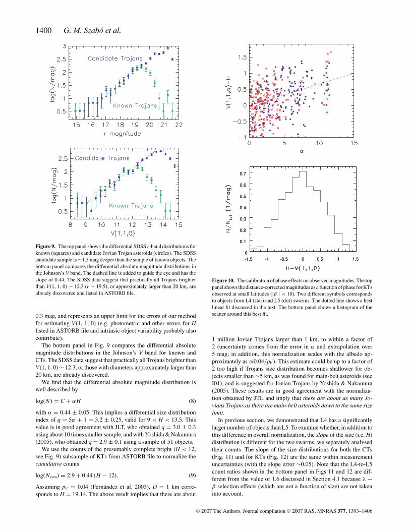
The differential apparent r-band magnitude distributions (forTrojans, Johnson’s V ∼ r + 0.25) for KTs and CTs are shownin the top panel in Fig. 9. The KT sample is complete to r ∼ 19.5,and the CT sample is complete to r ∼ 21. The formal cut-off for in-clusion of moving objects in the SDSS MOC is r < 21.5. A slightly

brighter completeness limit for Trojans can be understood as the re-moval of objects from a fairly narrow velocity space due to velocityerrors (see fig. 6 from I01). Because the CT sample is complete toa ∼1.5 mag deeper limit, it contains ∼4 times more objects. It isnoteworthy that the high completeness of KT sample indicated bythe SDSS data (i.e. the counts are practically identical for r < 19.5)argues that selection effects cannot be invoked to explain the L4–L5asymmetry in the number counts of Trojans with known orbits listedin Bowell’s ASTORB file.

In order to investigate the dependence of various quantities (suchas counts and colours) on object size, we transform apparent mag-nitudes to absolute magnitudes as follows. The dependence of ap-parent magnitude in the Johnson V band on absolute magnitude, H,distance from Sun, R, distance from Earth, , and viewing (phase)angle, α, can be expressed as

V (R, , α) = H + 5 log(R ) + F(α). (3)

Here V(R, , α) = r + 0.44(g − r) is synthesized from SDSSmeasurements, F(α) is the phase function, and H includes the de-pendence on diameter D (in km) and the V-band albedo, pV ,

H = 19.14 − 2.5 log( pV

0.04

)− 5 log(D). (4)

Note that formally V(1, 1, 0) = H. Given R and φ, and α can befound from

2 + 2 cos(φ) + 1 = R2 (5)



Figure 8. The top panel shows the observed surface density of KT asteroids from Bowell’s ASTORB file, analogously to Fig. 7. The distribution for each swarmis well described by a two-dimensional Gaussian. The second panel shows a model distribution that has the same shape as the Gaussian distribution impliedby the top panel, but normalized to the observed counts of SDSS CT (for each swarm separately), shown in the third panel with the same colour scheme (redcorresponds to 5 objects per deg2). The best-fitting L4:L5 number ratio is 1.6 ± 0.1. The difference between the observed counts and this model distribution,normalized by the Poisson error bars, is shown in the bottom panel (the purple regions contain no data). The value of χ2 per degree of freedom is 1.15.

and

α = φ − arccos

(1 + cos(φ)

R

). (6)

When applying this procedure to observations discussed here, Rand F(α) are not known. We adopt5 R = 5.2 au and model the phasefunction as F(α) = k |α|. Therefore,

H ∼ V (1, 1, 0) = V (1, 1, α) − k|α|. (7)

In order to determine coefficient k, we used KT asteroids ob-served at low latitudes (|β| < 10). A least-squares best fit to the

5 I01 developed a method for estimating heliocentric distance of asteroidsfrom their angular velocity measured by SDSS that is accurate to about 10per cent for main-belt asteroids. For Trojans, which have larger velocityerrors, a smaller error is introduced by assuming a constant R.

observed dependence of V(1, 1, α) − H on |α| gives k = 0.066± 0.018. To the zeroth order, the transformation from apparent toabsolute magnitudes for Trojans observed close to the oppositionamounts to a shift of about 7 mag. In order to distinguish absolutemagnitude for objects with known orbits from the estimates evalu-ated here, we will refer to H and V(1, 1, 0) for KT and CT samples,respectively.

It is noteworthy that the intercept of the best-fitting line discussedabove (see Fig. 10) is consistent with 0. This shows that the V-bandmagnitudes synthesized from SDSS photometry and H magnitudesfor Trojans listed in ASTORB file are expressed on the same photo-metric system. This appears not be the case for a significant fractionof main-belt asteroids whose magnitudes (that are simply adoptedfrom a variety of asteroid surveys) can have systematic errors aslarge as 0.5 mag (for more details see J02). The rms width ofthe residuals distribution shown in the bottom panel in Fig. 10 is



Figure 9. The top panel shows the differential SDSS r-band distributions forknown (squares) and candidate Jovian Trojan asteroids (circles). The SDSScandidate sample is ∼1.5 mag deeper than the sample of known objects. Thebottom panel compares the differential absolute magnitude distributions inthe Johnson’s V band. The dashed line is added to guide the eye and has theslope of 0.44. The SDSS data suggest that practically all Trojans brighterthan V(1, 1, 0) ∼ 12.3 (r ∼ 19.5), or approximately larger than 20 km, arealready discovered and listed in ASTORB file.

0.3 mag, and represents an upper limit for the errors of our methodfor estimating V(1, 1, 0) (e.g. photometric and other errors for Hlisted in ASTORB file and intrinsic object variability probably alsocontribute).

The bottom panel in Fig. 9 compares the differential absolutemagnitude distributions in the Johnson’s V band for known andCTs. The SDSS data suggest that practically all Trojans brighter thanV(1, 1, 0) ∼ 12.3, or those with diameters approximately larger than20 km, are already discovered.

We find that the differential absolute magnitude distribution iswell described by

log(N ) = C + αH (8)

with α = 0.44 ± 0.05. This implies a differential size distributionindex of q = 5α + 1 = 3.2 ± 0.25, valid for 9 < H < 13.5. Thisvalue is in good agreement with JLT, who obtained q = 3.0 ± 0.3using about 10 times smaller sample, and with Yoshida & Nakamura(2005), who obtained q = 2.9 ± 0.1 using a sample of 51 objects.

We use the counts of the presumably complete bright (H < 12,see Fig. 9) subsample of KTs from ASTORB file to normalize thecumulative counts

log(Ncum) = 2.9 + 0.44 (H − 12). (9)

Assuming pV = 0.04 (Fernandez et al. 2003), D = 1 km corre-sponds to H = 19.14. The above result implies that there are about

-1.5 -1 -0.5 0 0.5 1 1.50

0.1

0.2

0.3

0.4

0.5

0.6

0.7

-1.5 -1 -0.5 0 0.5 1 1.50

0.1

0.2

0.3

0.4

0.5

0.6

0.7

Figure 10. The calibration of phase effects on observed magnitudes. The toppanel shows the distance-corrected magnitudes as a function of phase for KTsobserved at small latitudes (|β | < 10). Two different symbols correspondsto objects from L4 (star) and L5 (dot) swarms. The dotted line shows a bestlinear fit discussed in the text. The bottom panel shows a histogram of thescatter around this best fit.

1 million Jovian Trojans larger than 1 km, to within a factor of2 (uncertainty comes from the error in α and extrapolation over5 mag; in addition, this normalization scales with the albedo ap-proximately as ∝0.04/pV ). This estimate could be up to a factor of2 too high if Trojans size distribution becomes shallower for ob-jects smaller than ∼5 km, as was found for main-belt asteroids (seeI01), and is suggested for Jovian Trojans by Yoshida & Nakamura(2005). These results are in good agreement with the normaliza-tion obtained by JTL and imply that there are about as many Jo-vians Trojans as there are main-belt asteroids down to the same sizelimit.

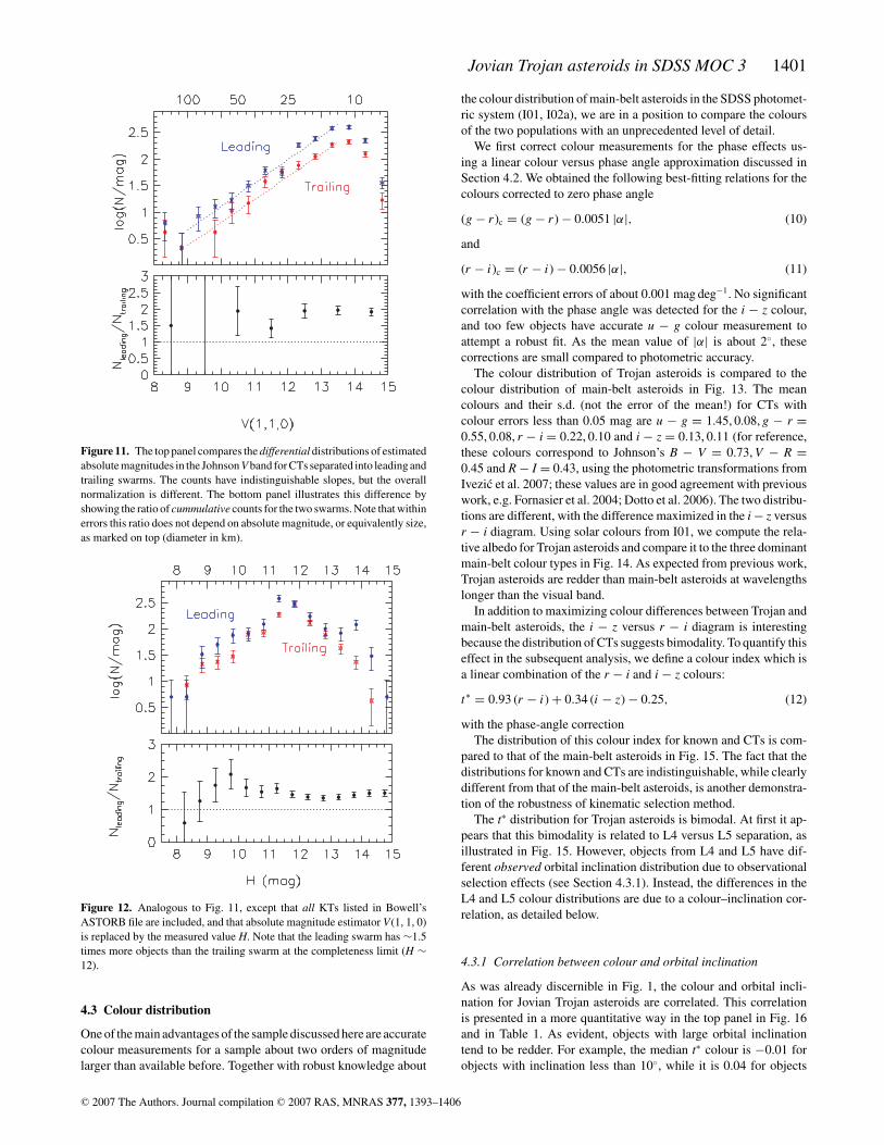
In previous section, we demonstrated that L4 has a significantlylarger number of objects than L5. To examine whether, in addition tothis difference in overall normalization, the slope of the size (i.e. H)distribution is different for the two swarms, we separately analysedtheir counts. The slope of the size distributions for both the CTs(Fig. 11) and for KTs (Fig. 12) are the same within measurementuncertainties (with the slope error ∼0.05). Note that the L4-to-L5count ratios shown in the bottom panel in Figs 11 and 12 are dif-ferent from the value of 1.6 discussed in Section 4.1 because λ −β selection effects (which are not a function of size) are not takeninto account.



Figure 11. The top panel compares the differential distributions of estimatedabsolute magnitudes in the Johnson V band for CTs separated into leading andtrailing swarms. The counts have indistinguishable slopes, but the overallnormalization is different. The bottom panel illustrates this difference byshowing the ratio of cummulative counts for the two swarms. Note that withinerrors this ratio does not depend on absolute magnitude, or equivalently size,as marked on top (diameter in km).

Figure 12. Analogous to Fig. 11, except that all KTs listed in Bowell’sASTORB file are included, and that absolute magnitude estimator V(1, 1, 0)is replaced by the measured value H. Note that the leading swarm has ∼1.5times more objects than the trailing swarm at the completeness limit (H ∼12).

4.3 Colour distribution

One of the main advantages of the sample discussed here are accuratecolour measurements for a sample about two orders of magnitudelarger than available before. Together with robust knowledge about

the colour distribution of main-belt asteroids in the SDSS photomet-ric system (I01, I02a), we are in a position to compare the coloursof the two populations with an unprecedented level of detail.

We first correct colour measurements for the phase effects us-ing a linear colour versus phase angle approximation discussed inSection 4.2. We obtained the following best-fitting relations for thecolours corrected to zero phase angle

(g − r )c = (g − r ) − 0.0051 |α|, (10)

and

(r − i)c = (r − i) − 0.0056 |α|, (11)

with the coefficient errors of about 0.001 mag deg−1. No significantcorrelation with the phase angle was detected for the i − z colour,and too few objects have accurate u − g colour measurement toattempt a robust fit. As the mean value of |α| is about 2◦, thesecorrections are small compared to photometric accuracy.

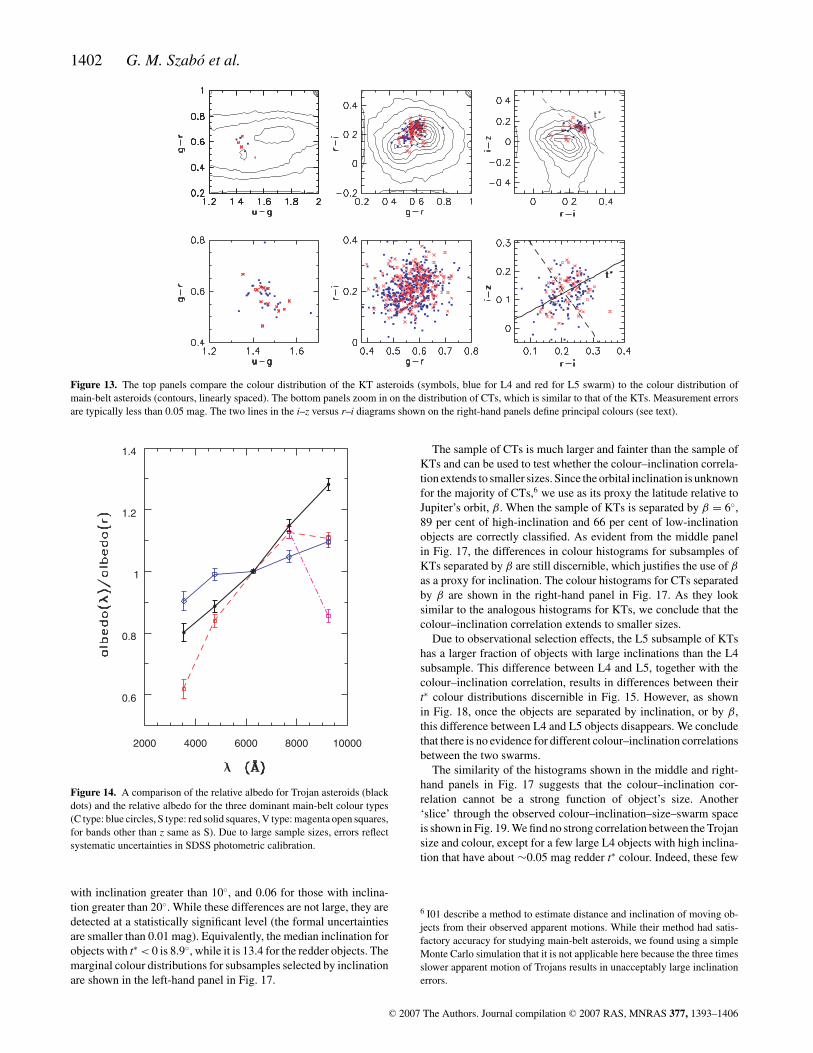
The colour distribution of Trojan asteroids is compared to thecolour distribution of main-belt asteroids in Fig. 13. The meancolours and their s.d. (not the error of the mean!) for CTs withcolour errors less than 0.05 mag are u − g = 1.45, 0.08, g − r =0.55, 0.08, r − i = 0.22, 0.10 and i − z = 0.13, 0.11 (for reference,these colours correspond to Johnson’s B − V = 0.73, V − R =0.45 and R − I = 0.43, using the photometric transformations fromIvezic et al. 2007; these values are in good agreement with previouswork, e.g. Fornasier et al. 2004; Dotto et al. 2006). The two distribu-tions are different, with the difference maximized in the i − z versusr − i diagram. Using solar colours from I01, we compute the rela-tive albedo for Trojan asteroids and compare it to the three dominantmain-belt colour types in Fig. 14. As expected from previous work,Trojan asteroids are redder than main-belt asteroids at wavelengthslonger than the visual band.

In addition to maximizing colour differences between Trojan andmain-belt asteroids, the i − z versus r − i diagram is interestingbecause the distribution of CTs suggests bimodality. To quantify thiseffect in the subsequent analysis, we define a colour index which isa linear combination of the r − i and i − z colours:

t∗ = 0.93 (r − i) + 0.34 (i − z) − 0.25, (12)

with the phase-angle correctionThe distribution of this colour index for known and CTs is com-

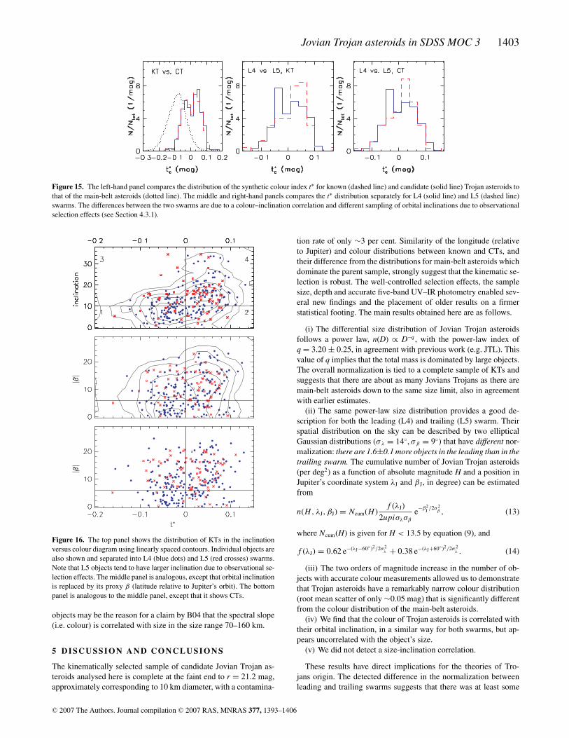
pared to that of the main-belt asteroids in Fig. 15. The fact that thedistributions for known and CTs are indistinguishable, while clearlydifferent from that of the main-belt asteroids, is another demonstra-tion of the robustness of kinematic selection method.

The t∗ distribution for Trojan asteroids is bimodal. At first it ap-pears that this bimodality is related to L4 versus L5 separation, asillustrated in Fig. 15. However, objects from L4 and L5 have dif-ferent observed orbital inclination distribution due to observationalselection effects (see Section 4.3.1). Instead, the differences in theL4 and L5 colour distributions are due to a colour–inclination cor-relation, as detailed below.

4.3.1 Correlation between colour and orbital inclination

As was already discernible in Fig. 1, the colour and orbital incli-nation for Jovian Trojan asteroids are correlated. This correlationis presented in a more quantitative way in the top panel in Fig. 16and in Table 1. As evident, objects with large orbital inclinationtend to be redder. For example, the median t∗ colour is −0.01 forobjects with inclination less than 10◦, while it is 0.04 for objects



Figure 13. The top panels compare the colour distribution of the KT asteroids (symbols, blue for L4 and red for L5 swarm) to the colour distribution ofmain-belt asteroids (contours, linearly spaced). The bottom panels zoom in on the distribution of CTs, which is similar to that of the KTs. Measurement errorsare typically less than 0.05 mag. The two lines in the i–z versus r–i diagrams shown on the right-hand panels define principal colours (see text).

2000 4000 6000 8000 10000

0.6

0.8

1

1.2

1.4

Figure 14. A comparison of the relative albedo for Trojan asteroids (blackdots) and the relative albedo for the three dominant main-belt colour types(C type: blue circles, S type: red solid squares, V type: magenta open squares,for bands other than z same as S). Due to large sample sizes, errors reflectsystematic uncertainties in SDSS photometric calibration.

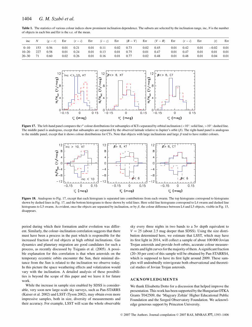
with inclination greater than 10◦, and 0.06 for those with inclina-tion greater than 20◦. While these differences are not large, they aredetected at a statistically significant level (the formal uncertaintiesare smaller than 0.01 mag). Equivalently, the median inclination forobjects with t∗ < 0 is 8.9◦, while it is 13.4 for the redder objects. Themarginal colour distributions for subsamples selected by inclinationare shown in the left-hand panel in Fig. 17.

The sample of CTs is much larger and fainter than the sample ofKTs and can be used to test whether the colour–inclination correla-tion extends to smaller sizes. Since the orbital inclination is unknownfor the majority of CTs,6 we use as its proxy the latitude relative toJupiter’s orbit, β. When the sample of KTs is separated by β = 6◦,89 per cent of high-inclination and 66 per cent of low-inclinationobjects are correctly classified. As evident from the middle panelin Fig. 17, the differences in colour histograms for subsamples ofKTs separated by β are still discernible, which justifies the use of β

as a proxy for inclination. The colour histograms for CTs separatedby β are shown in the right-hand panel in Fig. 17. As they looksimilar to the analogous histograms for KTs, we conclude that thecolour–inclination correlation extends to smaller sizes.

Due to observational selection effects, the L5 subsample of KTshas a larger fraction of objects with large inclinations than the L4subsample. This difference between L4 and L5, together with thecolour–inclination correlation, results in differences between theirt∗ colour distributions discernible in Fig. 15. However, as shownin Fig. 18, once the objects are separated by inclination, or by β,this difference between L4 and L5 objects disappears. We concludethat there is no evidence for different colour–inclination correlationsbetween the two swarms.

The similarity of the histograms shown in the middle and right-hand panels in Fig. 17 suggests that the colour–inclination cor-relation cannot be a strong function of object’s size. Another‘slice’ through the observed colour–inclination–size–swarm spaceis shown in Fig. 19. We find no strong correlation between the Trojansize and colour, except for a few large L4 objects with high inclina-tion that have about ∼0.05 mag redder t∗ colour. Indeed, these few

6 I01 describe a method to estimate distance and inclination of moving ob-jects from their observed apparent motions. While their method had satis-factory accuracy for studying main-belt asteroids, we found using a simpleMonte Carlo simulation that it is not applicable here because the three timesslower apparent motion of Trojans results in unacceptably large inclinationerrors.



Figure 15. The left-hand panel compares the distribution of the synthetic colour index t∗ for known (dashed line) and candidate (solid line) Trojan asteroids tothat of the main-belt asteroids (dotted line). The middle and right-hand panels compares the t∗ distribution separately for L4 (solid line) and L5 (dashed line)swarms. The differences between the two swarms are due to a colour–inclination correlation and different sampling of orbital inclinations due to observationalselection effects (see Section 4.3.1).

Figure 16. The top panel shows the distribution of KTs in the inclinationversus colour diagram using linearly spaced contours. Individual objects arealso shown and separated into L4 (blue dots) and L5 (red crosses) swarms.Note that L5 objects tend to have larger inclination due to observational se-lection effects. The middle panel is analogous, except that orbital inclinationis replaced by its proxy β (latitude relative to Jupiter’s orbit). The bottompanel is analogous to the middle panel, except that it shows CTs.

objects may be the reason for a claim by B04 that the spectral slope(i.e. colour) is correlated with size in the size range 70–160 km.

5 D I S C U S S I O N A N D C O N C L U S I O N S

The kinematically selected sample of candidate Jovian Trojan as-teroids analysed here is complete at the faint end to r = 21.2 mag,approximately corresponding to 10 km diameter, with a contamina-

tion rate of only ∼3 per cent. Similarity of the longitude (relativeto Jupiter) and colour distributions between known and CTs, andtheir difference from the distributions for main-belt asteroids whichdominate the parent sample, strongly suggest that the kinematic se-lection is robust. The well-controlled selection effects, the samplesize, depth and accurate five-band UV–IR photometry enabled sev-eral new findings and the placement of older results on a firmerstatistical footing. The main results obtained here are as follows.

(i) The differential size distribution of Jovian Trojan asteroidsfollows a power law, n(D) ∝ D−q , with the power-law index ofq = 3.20 ± 0.25, in agreement with previous work (e.g. JTL). Thisvalue of q implies that the total mass is dominated by large objects.The overall normalization is tied to a complete sample of KTs andsuggests that there are about as many Jovians Trojans as there aremain-belt asteroids down to the same size limit, also in agreementwith earlier estimates.

(ii) The same power-law size distribution provides a good de-scription for both the leading (L4) and trailing (L5) swarm. Theirspatial distribution on the sky can be described by two ellipticalGaussian distributions (σλ = 14◦, σβ = 9◦) that have different nor-malization: there are 1.6±0.1 more objects in the leading than in thetrailing swarm. The cumulative number of Jovian Trojan asteroids(per deg2) as a function of absolute magnitude H and a position inJupiter’s coordinate system λJ and βJ, in degree) can be estimatedfrom

n(H , λJ, βJ) = Ncum(H )f (λJ)

2upiσλσβ

e−β2J /2σ 2

β , (13)

where Ncum(H) is given for H < 13.5 by equation (9), and

f (λJ) = 0.62 e−(λJ−60◦)2/2σ 2λ + 0.38 e−(λJ+60◦)2/2σ 2

λ . (14)

(iii) The two orders of magnitude increase in the number of ob-jects with accurate colour measurements allowed us to demonstratethat Trojan asteroids have a remarkably narrow colour distribution(root mean scatter of only ∼0.05 mag) that is significantly differentfrom the colour distribution of the main-belt asteroids.

(iv) We find that the colour of Trojan asteroids is correlated withtheir orbital inclination, in a similar way for both swarms, but ap-pears uncorrelated with the object’s size.

(v) We did not detect a size-inclination correlation.

These results have direct implications for the theories of Tro-jans origin. The detected difference in the normalization betweenleading and trailing swarms suggests that there was at least some



Table 1. The statistics of various colour indices show prominent inclination dependence. The subsets are selected by the inclination range, inc, N is the numberof objects in each bin and Err is the s.e. of the mean.

inc N 〈g − r〉 Err 〈r − i〉 Err 〈i − z〉 Err 〈B − V〉 Err 〈V − R〉 Err 〈r − i〉 Err 〈t〉 Err

0–10 153 0.56 0.01 0.21 0.01 0.11 0.02 0.73 0.02 0.45 0.01 0.42 0.01 −0.02 0.0110–20 227 0.58 0.01 0.24 0.01 0.13 0.01 0.75 0.01 0.47 0.01 0.47 0.01 0.01 0.0120–30 71 0.60 0.02 0.26 0.01 0.16 0.01 0.77 0.02 0.48 0.01 0.48 0.01 0.04 0.01

Figure 17. The left-hand panel compares the t∗ colour distributions for subsamples of KTs separated by orbital inclination (<10◦: solid line, >10◦: dashed line.The middle panel is analogous, except that subsamples are separated by the observed latitude relative to Jupiter’s orbit (β). The right-hand panel is analogousto the middle panel, except that it shows colour distributions for CTs. Note that objects with large inclinations and large β tend to have redder colours.

Figure 18. Analogous to Fig. 17, except that each histogram is separated into contributions from each swarm. The top histograms correspond to histogramsshown by dashed lines in Fig. 17, and the bottom histograms to those shown by solid lines. Here solid line histograms correspond to L4 swarm and dashed linehistograms to L5 swarm. As evident, once the objects are separated by inclination, or by β, the colour difference between L4 and L5 objects, visible in Fig. 15,disappears.

period during which their formation and/or evolution was differ-ent. Similarly, the colour–inclination correlation suggests that theremust have been a process in the past which is responsible for theincreased fraction of red objects at high orbital inclinations. Gasdynamics and planetary migration are good candidates for such aprocess, as recently discussed by Tsiganis et al. (2005). A possi-ble explanation for this correlation is that when asteroids on thetemporary eccentric orbits encounter the Sun, their minimal dis-tance from the Sun is related to the inclination we observe today.In this picture the space weathering effects and volatization wouldvary with the inclination. A detailed analysis of these possibili-ties is beyond the scope of this paper and we leave it for futurework.

While the increase in sample size enabled by SDSS is consider-able, very soon new large-scale sky surveys, such as Pan-STARRS(Kaiser et al. 2002) and LSST (Tyson 2002), may obtain even moreimpressive samples, both in size, diversity of measurements andtheir accuracy. For example, LSST will scan the whole observable

sky every three nights in two bands to a 5σ depth equivalent toV = 25 (about 2.5 mag deeper than SDSS). Using the size distri-bution determined here, we estimate that LSST, which may haveits first light in 2014, will collect a sample of about 100 000 JovianTrojan asteroids and provide both orbits, accurate colour measure-ments and light curves for the majority of them. A significant fraction(20–30 per cent) of this sample will be obtained by Pan-STARRS4,which is supposed to have its first light around 2009. These sam-ples will undoubtedly reinvigorate both observational and theoreti-cal studies of Jovian Trojan asteroids.

AC K N OW L E D G M E N T S

We thank Elisabetta Dotto for a discussion that helped improve thepresentation. This work has been supported by the Hungarian OTKAGrants T042509, the ‘Magyary Zoltan’ Higher Educational PublicFoundation and the Szeged Observatory Foundation. We acknowl-edge generous support by Princeton University.



-0.2

-0.15

-0.1

-0.05

0

0.05

0.1

0.15

0.2

10 11 12 13 14

t*

V(1,1,0)

CT, L4, low

-0.2

-0.15

-0.1

-0.05

0

0.05

0.1

0.15

0.2

10 11 12 13 14

t*

V(1,1,0)

CT, L4, high

-0.2

-0.15

-0.1

-0.05

0

0.05

0.1

0.15

0.2

10 11 12 13 14

t*

V(1,1,0)

CT, L5, low

-0.2

-0.15

-0.1

-0.05

0

0.05

0.1

0.15

0.2

10 11 12 13 14t*

V(1,1,0)

CT, L5, high

Figure 19. Colour–magnitude diagrams for subsamples of CTs separated into L4 (top) and L5 (bottom) objects, and further into low-inclination (left-handpanels) and high-inclination (right-hand panels) objects. Small dots represent individual objects and large circles are the median values of t∗ colour in 1-magwide bins of absolute magnitude. The 1σ envelope around the median values is computed from the interquartile range. Note the cluster of V(1, 1, 0) < 11objects in top right-hand panel that have slightly redder objects than the rest of the sample.

Funding for the SDSS and SDSS-II has been provided by the Al-fred P. Sloan Foundation, the Participating Institutions, the NationalScience Foundation, the US Department of Energy, the NationalAeronautics and Space Administration, the Japanese Monbuka-gakusho, the Max Planck Society and the Higher Education FundingCouncil for England. The SDSS website is http://www.sdss.org/.

The SDSS is managed by the Astrophysical Research Consortiumfor the Participating Institutions. The Participating Institutions arethe American Museum of Natural History, Astrophysical InstitutePotsdam, University of Basel, University of Cambridge, Case West-ern Reserve University, University of Chicago, Drexel University,Fermilab, the Institute for Advanced Study, the Japan ParticipationGroup, Johns Hopkins University, the Joint Institute for Nuclear As-trophysics, the Kavli Institute for Particle Astrophysics and Cosmol-ogy, the Korean Scientist Group, the Chinese Academy of Sciences(LAMOST), Los Alamos National Laboratory, the Max-Planck-Institute for Astronomy (MPIA), the Max-Planck-Institute for As-trophysics (MPA), New Mexico State University, Ohio State Univer-sity, University of Pittsburgh, University of Portsmouth, PrincetonUniversity, the United States Naval Observatory and the Universityof Washington.

R E F E R E N C E S

Abazajian K. et al., 2003, AJ, 126, 2081Bendjoya P., Cellino A., di Martino M., Saba L., 2004, Icarus, 168, 374

(B04)Bowell E., 2001, Introduction to ASTORB, available from

ftp://ftp.lowell.edu/pub/elgb/astorb.htmlDotto E. et al., 2006, Icarus, 183, 420Fernandez Y. R., Sheppard S. S., Jewitt D. C., 2003, AJ, 126, 1563

Fitzsimmons A., Dahlgren M., Lagerkvist C.-I., Magnusson P., Williams L.P., 1994, A&A, 282, 634

Fornasier S., Dotto E., Marzari F., Barucci M. A., Boehnhardt H., HainautO., de Bergh C., 2004, Icarus, 172, 221

Fukugita M., Ichikawa T., Gunn J. E., Doi M., Shimasaku K., Schneider D.P., 1996, AJ, 111, 1748

Gomes R. S., 1998, AJ, 116, 2590Gunn J. E. et al., 1998, AJ, 116, 3040Hogg D. W., Finkbeiner D. P., Schlegel D. J., Gunn J. E., 2002, AJ, 122,

2129Ivezic Z. et al., 2001, AJ, 122, 2749 (I01)Ivezic Z., Juric M., Lupton R. H., Tabachnik S., Quinn T., 2002a, AJ, 124,

2943 (I02a)Ivezic Z., Juric M., Lupton R. H., Tabachnik S., Quinn T., 2002b, Proc. SPIE,

4836, 98Ivezic Z. et al., 2004, Astron. Nachr. 325, 583Ivezic Z. et al., 2007, in Sterken C., ed., ASP Conf. Proc. Vol. 364, The Future

of Photometric, Spectrophotometric and Polarimetric Standardization.Astron. Soc. Pac., San Francisco, p. 165

Jedicke R., Nesvorny D., Whiteley R., Ivezic Z., Juric M., 2004, Nat, 429,275

Jewitt D. C., 1996, Earth, Moon & Planets, 72, 185Jewitt D. C., Luu J. X., 1990, AJ, 100, 933Jewitt D. C., Trujillo C. A., Luu J. X., 2000, AJ, 120, 1140 (JTL)Juric M. et al., 2002, AJ, 124, 1776 (J02)Kaiser N. et al., 2002, Proc. SPIE, 4836, 154Lupton R. H. et al., 2001, in Harnden F. R., Jr, Primini F. A., Payne H. E. M.,

eds, ASP Conf. Proc. Vol. 238, Astronomical Data Analysis Softwareand Systems X. Astron. Soc. Pac., San Francisco, p. 269

Lupton R. H., Ivezic Z., Gunn J. E., Knapp G. R., Strauss M. A., Yasuda N.,2002, Proc. SPIE, 4836, p. 350

Marzari F., Scholl H., Murray C., Lagerkvist C., 2002, in Bottke W. F.,Cellino A., Paolicchi P., Binzel R. P., eds, Asteroids III. Univ. ArizonaPress, Tucson, p. 725



Milani A., 1999, Icarus, 137, 269Morbidelli A., Levison H. F., Tsiganis K., Gomes R., 2005, Nat, 435, 462Nesvorny D., Jedicke R., Whiteley R., Ivezic Z., 2005, Icarus, 173, 132Peale S. J., 1993, Icarus, 106, 308Pier J. R., Munn J. A., Hindsley R. B., Hennesy G. S., Kent S. M., Lupton

R. H., Ivezic Z., 2003, AJ, 125, 1559Shoemaker E. M., Shoemaker C. S., Wolfe R. F., 1989, in Binzel R. P.,

Gehrels T., Matthews M. S., eds, Asteroids II. Univ. Arizona Press,Tucson, p. 487

Smith J. A. et al., 2002, AJ, 123, 2121Szabo Gy. M., Ivezic Z., Juric M., Lupton R., Kiss L. L., 2004, MNRAS,

348, 987

Tedesco E. F., 1989, in Binzel R. P., Gehrels T., Matthews M. S., eds, Aster-oids II. Univ. Arizona Press, Tucson, p. 1090

Tedesco E. F., Cellino A., Zappala V., 2005, AJ, 129, 2869Tsiganis K., Gomes R., Morbidelli A., Levison H. F., 2005, Nat, 435, 462Tyson J. A., 2002, Proc. SPIE, 4836, 10York D. G. et al., 2000, AJ, 120, 1579Yoshida F., Nakamura T., 2005, AJ, 130, 2900Zellner B., Tholen D. J., Tedesco E. F., 1985, Icarus, 61, 355

This paper has been typeset from a TEX/LATEX file prepared by the author.


the properties of jovian trojan asteroids listed in sdss...

Documents