the price of gasoline and the demand for fuel efficiency e monthly
TRANSCRIPT
THE PRICE OF GASOLINE AND THE DEMAND FOR FUEL EFFICIENCY: EVIDENCE FROM MONTHLY NEW VEHICLES SALES DATA*
Thomas Klier Federal Reserve Bank of Chicago
Joshua Linn Department of Economics
University of Illinois at Chicago [email protected]
September 2008
ABSTRACT
This paper uses a unique data set of monthly new vehicle sales by detailed model from 1970-2007, and implements a new identification strategy to estimate the effect of gasoline prices on new vehicle demand. We control for unobserved vehicle and consumer characteristics by using within model-year changes in gasoline prices and vehicle sales. We find a significant demand response, as nearly half of the decline in market share of U.S. manufacturers from 2002-2007 was due to the increase in gasoline prices. On the other hand, a gasoline tax increase would have a modest effect on average fuel efficiency.
* We thank participants at the UCLA Environmental Economics Workshop, the International Industrial Organization Conference, the Midwest Economic Association and the Federal Reserve System Committee on Regional Analysis Meeting. Taft Foster, Vincent Liu and Cristina Miller provided excellent research assistance.

2
1 INTRODUCTION
The rapid rise in the price of gasoline from just over $1 at the beginning of 2002 to over $4 by
mid 2008 has renewed interest in the relationship between the price of gasoline and the demand
for fuel efficient vehicles in the U.S. market. Recent research on oil prices and economic activity
suggests that because of improved energy efficiency, the U.S. economy as a whole is currently
much less sensitive to oil prices than it was prior to the 1970s oil shocks (Hooker, 1996 and
Linn, 2008). In contrast, recent events suggest that U.S. automakers may remain quite sensitive
to oil and gasoline prices.
Many industry analysts and the popular press have noted the large decrease in sales for U.S.
automakers and large SUVs over the past six years, and have widely attributed some of the
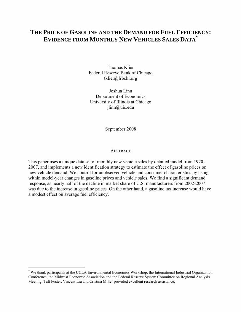
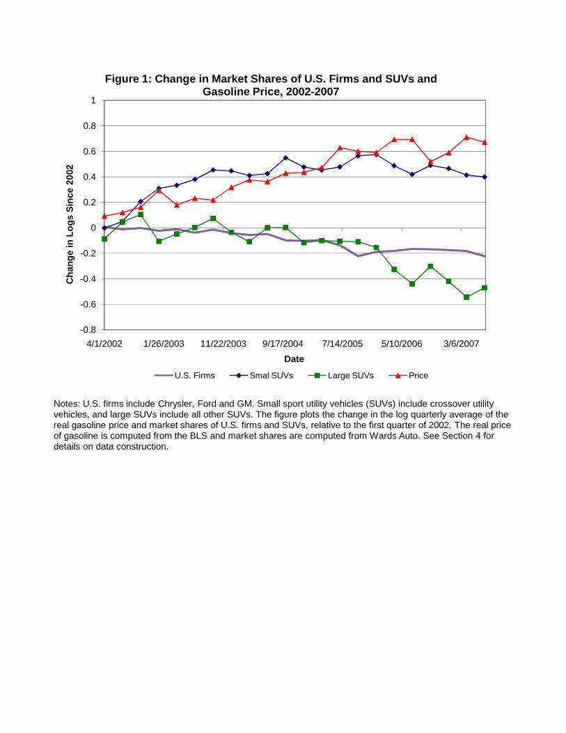
changes to the coinciding increase in the price of gasoline. Figure 1 depicts these trends, showing
a 20 percent decrease in the market share of U.S. firms between 2002 and 2007, which represents
several billion dollars per year in lost profits.1 The figure also suggests that some of the decrease
in sales by U.S. firms can be attributed to changes in the SUV segment of the market. At the
beginning of this time period, U.S. firms accounted for 80 percent of sales of large SUVs (with a
mean fuel efficiency of 16.6 miles per gallon), but only 37 percent of sales of smaller SUVs
(commonly called crossover utility vehicles, with a mean fuel efficiency of 22.2 miles per
gallon). The market share of small SUVs has increased at the expense of the market share of
large SUVs, and at the same time the real price of gasoline has nearly doubled. Although the
contemporaneous correlations between the price of gasoline and market shares are suggestive, it
must be recalled that fuel costs are only a fraction of the total cost of the vehicle, and that many
1 The market share of U.S. automakers had been declining since the mid 1960s. After stabilizing for most of the 1980s and the early 1990s, it started declining again in 1997.
3
other factors could explain these trends. In fact, despite the attention given to gasoline prices by
the press, there has not been a rigorous analysis of the extent two which increases in gasoline
prices adversely affect U.S. automakers.
The effect of the price of gasoline on new vehicle demand is also central to the ongoing
policy debate over reducing gasoline consumption, which has emanated from concerns about
global warming and reducing oil imports.2 In 2007, Congress passed legislation that increased
the CAFE standard by about 40 percent, to be effective by the year 2020. During the
Congressional debate over the bill, several members of Congress proposed an increase in the
gasoline tax or the introduction of a carbon tax as alternative means of reducing gasoline
consumption.3 The welfare effects of the CAFE standard and the gasoline tax, as well as the
optimal gasoline tax (Parry and Small, 2005), depend partly on the effect of the price of gasoline
on the demand for fuel efficient vehicles (Austin and Dinan, 2005).
Despite the large empirical literature on the effect of the price of gasoline on new vehicle
demand, the cause of the changes in market shares in Figure 1 and the effect of the gasoline tax
on average fuel efficiency remain as open questions. Previous studies focus on the effect of
gasoline prices on average fuel efficiency across the entire market, and thus do not shed light on
the causes of the changes in market shares depicted in Figure 1. Furthermore, as discussed in
more detail below, these studies do not control for both unobserved consumer and vehicle
characteristics, which may bias the estimated effect of the gasoline tax on average fuel
efficiency.
In this paper, we estimate the effect of the price of gasoline on the demand for fuel efficient
vehicles. We use a unique data set of monthly sales by vehicle model that spans nearly 40 years.
2 See, for example, hearings at the House Energy and Commerce committee on March 14, 2007. 3 During the summer of 2007, Congressman Dingell (MI) proposed a 50 cent per gallon gasoline tax increase (Timiraos, 2007)

4
The disaggregated and high-frequency data allow for a simple and transparent empirical strategy
that controls for unobserved consumer and vehicle characteristics. We find that gasoline prices
significantly affect the new vehicles market, as the recent price increase explains nearly half of
the decrease in market share of U.S. firms. On the other hand, a one dollar increase in the price
of gasoline would modestly increase fuel efficiency, by 0.5-1 miles per gallon, which is less than
some other recent estimates.
We now discuss the analysis and previous literature in more detail. The empirical strategy
addresses the limitations of the previous literature on the effect of the price of gasoline on new
vehicle demand. First, previous studies have not accounted for the potential correlation between
the price of gasoline and unobserved consumer and vehicle characteristics. Many studies rely
primarily on cross-sectional variation in gasoline prices (e.g., Goldberg, 1998, West, 2004 and
Bento et al., 2006), and thus depend on the questionable assumption that prices are uncorrelated
with unobserved consumer preferences (Chouinard and Perloff, 2007); for example, it is assumed
that environmentalists are no more likely to live in states with high gasoline taxes.4 The failure to
account for unobservables is particularly problematic because the direction of the resulting bias
cannot be determined from economic theory; unobserved vehicle and consumer characteristics
may be positively or negatively correlated with the price of gasoline. An additional limitation of
the cross-sectional analysis is that the relationship between the price of gasoline and the demand
for fuel efficient vehicles may have changed over time. Recent estimates of the elasticity of
gasoline consumption to the price of gasoline (e.g., Hughes et al., 2008) suggest that the
4 An earlier empirical literature estimated the effect of the price of gasoline on new vehicle demand in the 1970s (see Tardiff, 1980, for a summary). These studies have similar limitations to the more recent ones, however. For example, Boyd and Mellman (1980) find a large effect on demand using cross-sectional variation in vehicle characteristics and prices, but the study does not control for unobserved characteristics.

5
elasticity has decreased in magnitude. However, it is not known whether the effect of the price of
gasoline on the demand for fuel efficient vehicles has changed as well.
Furthermore, time series analysis of the price of gasoline on new vehicle demand only
partially addresses these issues (e.g., Small and Van Dender, 2007), because these studies use
market-level fuel economy measures and do not control for unobserved vehicle characteristics –
for example, weight and power are highly correlated with fuel efficiency. Finally, many earlier
studies analyze choices among broad vehicle classes, such as small and large cars. There is
substantial heterogeneity within classes, however, which implies that the full response may be
greater than these studies indicate.
This paper makes several advances beyond the existing literature. First, we use a unique data
set and empirical strategy. The data include monthly national sales by detailed vehicle model
from 1970-2007, including a new set of 1970s sales data compiled from print sources. As Berry,
Levinsohn and Pakes (1995) argue, when using market-level data it is necessary to account for
the potential correlation between vehicle prices, sales and unobserved vehicle and consumer
characteristics. The monthly frequency of the sales data allows for a simple linear estimating
equation that controls for these unobserved variables. The empirical strategy derives from the
details of automobile production, specifically, that unobserved vehicle characteristics do not vary
over the model-year, and the fact that consumer tastes are likely to be slow-moving and
uncorrelated with monthly variation of the price of gasoline. The empirical specification exploits
within model-year changes in the monthly price of gasoline and vehicle sales, while controlling
for unobserved characteristics.5 As discussed in more detail below, the potential drawback of this
5 Similarly to this paper, Busse et al. (2005) use within model-year changes in manufacturing incentives to estimate the effect of incentives on transaction prices. The authors use a regression discontinuity design to address the potential endogeneity of the incentives. In contrast, we assume that the price of gasoline is exogenous to these incentives, and discuss this assumption further in Sections 5 and 6.

6
approach is that we estimate the monthly effect of the price of gasoline on sales rather than a
long-run effect, which is important for understanding the causes of recent changes in market
shares as well as the effect of raising the gasoline tax. We investigate the long-run effect of the
price of gasoline on vehicle sales by including lags and controlling for demand shocks over the
previous year. We find that the short run and long run quantity effects are similar in magnitude,
validating our analysis and the interpretation of the empirical results.
The second contribution of this paper is that the sample period and unit of analysis allow us
to investigate a number of questions about gasoline prices and consumer demand that have not
been the focus of previous work. First, the model level data allow us to investigate the causes of
recent market trends shown in Figure 1. Second, we use the 37-year panel to consider whether
the relationship between gasoline prices and new vehicle demand has changed over time, or if
there are asymmetric or lagged demand responses.
The main results are reported in Section 5. The increase in the price of gasoline between
2002 and 2007 explains about 25 percent of the shift from large SUVs to small SUVs and 40
percent of the decrease in the market share of U.S. manufacturers. Thus, the results indicate that
the price of gasoline has a significant effect on the new vehicles market, but the effect is smaller
than is often suggested. We estimate that the elasticity of average new vehicle fuel efficiency
with respect to the price of gasoline is about 0.12, which is about half of the elasticity reported in
Austin and Dinan (2005). The elasticity implies that a one dollar increase in the price of gasoline
raises average fuel efficiency by 0.5-1 miles per gallon.
In comparison to previous studies, we investigate the importance of functional form
assumptions and show that the results are robust to using a number of different estimation
models. We also find that the demand response to the price of gasoline is greater when gasoline

7
prices are high. Finally, we find limited evidence of a lagged response to changes in the price of
gasoline and provide evidence in support of the assumption that the price of gasoline is
exogenous to consumer preferences.
2 CONCEPTUAL FRAMEWORK: THE PRICE OF GASOLINE AND NEW VEHICLE DEMAND
This section describes a model of consumer demand for new vehicles to illustrate the relationship
between the price of gasoline and equilibrium sales. We use a discrete choice model that is
similar to Berry, Levinsohn and Pakes (BLP). The market for new automobiles
contains J models, or varieties, with each model indexed by Jj ,...,1= . The market spans one
year, with months indexed by t . Individual i derives utility ijtU by purchasing model j in
month t according to:
ijtjjjtjjijt XfmpU εξβα +++++= )( . (1)
The purchase price of the model is jp , the expected maintenance costs are jm and the expected
fuel costs are jtf . These variables reduce available income and therefore utility, so α is negative.
The vector jX consists of attributes of the model that can be observed by the individual and
econometrician, such as engine size. The last two variables in equation (1) are the mean utility
from unobserved model attributes, jξ , and an individual- and model-specific error term. In
equation (1),α andβ are constant across models, which implies that the purchase price, operating
costs and attributes in the vector jX affect the utility of all consumers equally. This assumption is
stronger than the random coefficients specification of BLP, but will be relaxed below.
A central feature of equation (1) is that the vehicle’s price, expected maintenance costs, as
well as observed and unobserved characteristics, do not vary over the model-year and thus do not
8
have time subscripts. In contrast, expected fuel costs, which depend on the expected price of
gasoline, may vary by month. This framework is consistent with the typical production process
of new vehicles. For most vehicle lines, production begins in July or August after a brief, one- or
two-week, shutdown period. During that period, the manufacturer may change characteristics
such as engine size. In practice, changes across model-years range from very minor to a
complete overhaul. Once production begins, however, the features of a vehicle are constant over
the model-year; a 2005 Honda Civic purchased in September of 2004 is the same as a 2005 Civic
purchased in May of 2005. To simplify the notation we define a model-specific intercept that
does not vary over time: ijjjjjj Xmp εξβααφ ++++≡ . The intercept absorbs vehicle price,
maintenance costs, observed characteristics and mean unobserved characteristics, but does not
include fuel costs.
We characterize the market-level demand for each model in a straightforward manner. Each
consumer purchases one of the j models or the outside good, which we take to be a used vehicle.
Making the standard extreme value assumption for the residual error term yields the following
expression for the difference between the log market share of model j , jts , and the log market
share of the outside good ts0 :
jjttjt fss φα +=− 0lnln . (2)
Equation (2) is the standard aggregate logit equation with fixed effects, in which the market
share of model j depends negatively on expected fuel costs.
3 ESTIMATING THE EFFECT OF GASOLINE PRICES ON NEW VEHICLE DEMAND
This section describes the empirical strategy for estimating the effect of the price of gasoline on
the demand for fuel efficient vehicles. Previous work has used two approaches based on equation

9
(1). The first estimates a nested logit model, which requires assumptions about substitution
patterns across models and the exogeneity of the price of gasoline (e.g., West, 2004, and
McManus 2005). Alternatively, BLP uses market-level data and relies on a set of price
instruments as well as assumptions about the distributions of parameters and unobserved
characteristics. Our empirical strategy is an alternative to BLP. We use monthly sales data and
exploit the fact that vehicle characteristics do not change within the model-year.
The estimating equation is derived by adding time dummies to equation (2), which eliminates
the log market share of used goods on the left-hand side, and controls for substitution between
new and used vehicles (Knittel and Stango, 2008):
jtjytjtjt fs νφτα +++=ln . (3)
The model-year intercepts, jyφ , control for characteristics that do not change within the model-
year, such as engine characteristics.
Expected fuel costs are:
])1(
1[ sjy
gs
tT
tssjt M
MPGP
rf ∑
+
= += . (4)
Fuel costs in period s equal the number of miles driven, sM , multiplied by the cost of driving one
mile, jyg
s MPGP / , where gsP is the expected price of gasoline in period s and jyMPG is fuel
efficiency, in miles per gallon (MPG). Total expected fuel costs, jtf , equal discounted expected
fuel costs, with a discount rate of r and a vehicle life ofT periods.
We assume that the price of gasoline follows a random walk, so that the expected price at
time ts > is equal to the price at time t . As a result, the expected cost of driving a specific model

10
is proportional to the current price of gasoline, divided by the vehicle’s fuel efficiency. We use
equation (4) to replace jtf in equation (3):
jtjytjy
gt
jt MPGP
s νφτα +++=ln . (5)
Equation (5) is the baseline estimating equation. The dependent variable is the log share of sales
of model j in month t . The first independent variable, referred to as dollars-per-mile, is the
expected cost of driving the vehicle one mile at the time of purchase; gtP is the seasonally
adjusted price of gasoline; and jyMPG is the fuel efficiency of model j in model-year y. The next
section describes the details of the variable construction.
The coefficient of interest isα , which is proportional to the effect of the cost of driving one
mile on the log market share. The parameterα is identified by time-series variation of the price
of gasoline and cross-sectional variation of fuel efficiency. In particular, within-year variation of
the price of gasoline differentially affects expected driving costs across models. For example,
when the expected price of gasoline increases, the fuel costs of a fuel-efficient vehicle increase
by less than the costs of a “gas guzzler”.
The model-year intercepts and monthly gasoline price variation are central to the empirical
strategy. The model-year intercepts account for the potentially endogenous relationship between
the average retail price and vehicle characteristics (Nevo, 2000). They also allow for a different
coefficient on the average retail price for each model, thus avoiding the independence of
irrelevant alternatives (IIA) assumption that is commonly made in the standard logit model. Note
that in equation (5), the assumption thatα is constant across models has different implications
than a model in which the coefficient on the retail price is constant across models. Assuming
thatα is constant implies that when the price of gasoline changes, the difference in the change in

11
market shares for any two models is proportional to the difference in the inverse of the models’
fuel efficiencies. For example, an increase in the price of gasoline would cause SUV consumers
to substitute from large to small SUVs in the same proportion as would minivan consumers
substitute from large to small minivans. This seems to be a more reasonable assumption than the
IIA property, but will be relaxed below by allowingα to vary over time and across models.6
The final assumption is that the price of gasoline is exogenous to within model-year
determinants of sales. Copeland et al. (2005) and Corrado et al. (2006) have documented that
transaction prices (the prices paid by the consumer, as distinct from the manufacturer suggested
retail price, MSRP) vary substantially within the model-year. Prices decline dramatically over
the course of the model-year, and sales follow a “hump-shaped” pattern, peaking in the early
summer. Furthermore, sales and price profiles vary across market segments (e.g., compact cars),
and many manufacturers have recently introduced incentives for specific models (Busse et al.,
2007). These patterns are the result of complex inventory and vehicle production optimization
problems, and which we assume are uncorrelated with dollars-per-mile. Section 6 provides some
evidence in support of this assumption.
The motivation for estimatingα is that we can then address how much of the changes in
market shares in Figure 1 are due to the increase in gasoline prices and to estimate the effect of
the gasoline tax on average fuel efficiency. For example, to calculate the effect of the price
increase on SUV market shares, we use equation (5) to compute counterfactual market shares in
2007 using the price of gasoline in 2002; the effect of the price increase can be inferred from the
differences between actual and counterfactual market shares. Note that the denominator in the
6 Equation (5) includes several additional functional form assumptions: the vehicle price and driving costs are linear and separable in the utility function, there are no income effects, and the effect of an increase in fuel costs on utility is the same across all consumers. These assumptions are also relaxed below.

12
market share in equation (5) includes new and used vehicles. We are interested in the effect of
gasoline prices on new vehicle market shares, and therefore renormalize market shares to sum to
one when calculating the counterfactuals.
Before presenting the results, we argue thatα is the appropriate parameter for answering
these questions. As just discussed, we assume that the price of gasoline is exogenous to other
determinants of new vehicle demand. However, it is important to note that we allow for the
possibility that the price of gasoline affects new vehicle prices, as documented by Langer and
Miller (2008). In other words,α describes the equilibrium relationship between the price of
gasoline and new vehicle sales. An increase in the price of gasoline causes a relative outward
shift of the demand curves of fuel efficient vehicles and a movement along the corresponding
supply curves. The same price increase would cause a relative inward shift of the demand curves
for gas guzzlers. Note that both the market share and gas tax questions depend on the
relationship between the price of gasoline and equilibrium sales. Estimatingα , as opposed to
analyzing vehicle prices, is therefore sufficient for answering these questions.
However, these questions are long-run in nature. Because we utilize monthly data to estimate
equation (5), the estimate ofα corresponds to the short-run effect of the price of gasoline. Thus,
α depends on how much the demand curves for each vehicle model shift in the short run and on
the shape of the corresponding short-run supply curves. If supply curves have the same shapes
and demand curves shift by the same amounts in the long run as the short run, the effect of the
price of gasoline on new vehicle demand would not vary across time horizons. Of course, this
need not be the case. For example, see Bresnahan and Ramey (1993) and Copeland and Hall
(2005) on production and pricing decisions in the short and long run. Section 5 assesses the

13
relationship between the short- and long-run effects of the price of gasoline on new vehicle sales.
We find the two to be fairly similar, validating our approach. 7,8
4 DATA
We construct the real price of gasoline with data from the Bureau of Economic Analysis (BEA),
using the monthly consumer price index (CPI) and the price of gasoline from 1970-2007.9 The
real price of gasoline, gtP , is the price of gasoline divided by the CPI, with the CPI normalized to
one in April of 2008. The price of gasoline is seasonally adjusted using X-12 ARIMA, which is
the same model used by the Census Bureau.
Model sales are from weekly publications of Wards Automotive Reports (1970-1979) and
Ward’s AutoInfoBank (1980-2007). Note that the 1970s sales data do not include light trucks or
imports. We match monthly sales data by individual model from 1970 to 2007 to model
characteristics data.10 The characteristics data are available in print in the annual Ward’s
Automotive Yearbooks (1970-2007), and include wheelbase, curb weight, engine size
7 The price response may vary across firms if an increase in the price of gasoline relaxes the constraint imposed by the CAFE standard (Jacobsen, 2007). Estimating a separate α for each model-year allows for this possibility, and the results are unaffected (see Table 4). 8 From the model in Section 2,α is proportional to miles driven, which is defined as the number of miles driven per year, conditional on vehicle choice. The price of gasoline may affect miles driven, but consumers should account for this effect when making their purchase decisions. Consequently, α includes the indirect effect of the price of gasoline on sales via miles driven. 9 More specifically, the gasoline price is constructed from the price of regular unleaded gasoline, the price of regular leaded gasoline, and the nominal price of crude oil. The gasoline price equals the price of unleaded gasoline when the price is available, from 1976-2007. We impute the gasoline price before 1976 using the estimated relationship between the prices of unleaded gasoline, leaded gasoline and oil when the price series overlap. 10 The match is not straightforward because the two data sets are reported at different levels of aggregation. Vehicle characteristics data are reported at the “trim level” to recognize differences in the MSRP; for example, the data distinguish the 2- and 4-door versions of the Honda Accord sedan. We aggregate the characteristics data to match the model-based sales data, and calculate four statistical moments for the distribution of the vehicle characteristics by car line: minimum, maximum, mean and median. We use the mean value to estimate equation (5), but obtain similar results using other moments.

14
(displacement) and retail price. Note that the model-year is defined to begin in September for
each model.11
The fuel efficiency of each vehicle is obtained from the EPA for model-years 1978-2007.12
Fuel efficiency from 1970-1977 is imputed from the estimated relationship between fuel
efficiency, wheelbase, weight and engine size from 1978-1979. The imputation is valid under the
assumption that vehicle technology did not change in the 1970s, and may introduce some
measurement error.
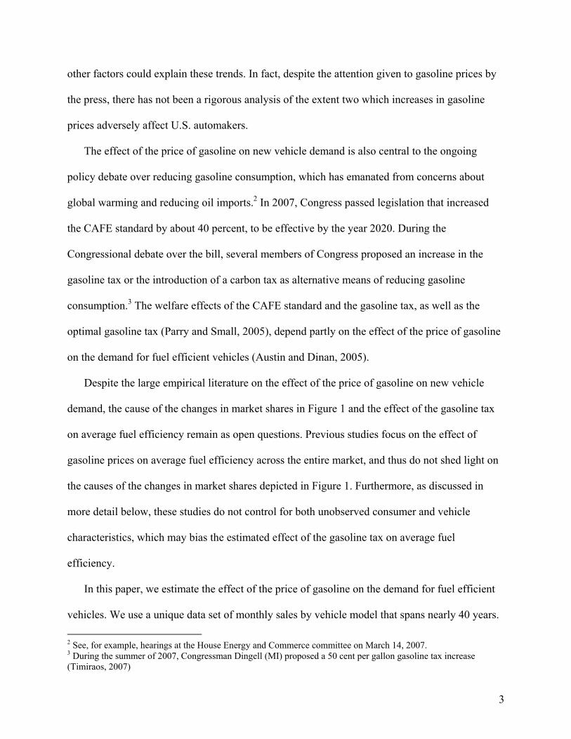
Figure 2a shows the real price of gasoline and the sales-weighted average MPG from 1970-
2007, plotting quarterly averages for clarity. Both series vary considerably over time. The price
of gasoline increased sharply in late 1973 and again in 1979, coinciding with the major oil
shocks, and declined significantly in the mid 1980s. The price was then relatively stable through
the 1990s, before increasing from 2002-2007. Average MPG declined gradually in the early
1970s and began increasing in the late 1970s and 1980s, as the CAFE standard, which took effect
in 1978, increased.13 Fuel efficiency declined steadily in the 1990s, remaining roughly constant
thereafter. Much of the decrease was due to compositional changes, particularly the increase in
sales of SUVs, which were subject to the lower CAFE standard for light trucks.
Figure 2b shows the log price of gasoline and log average fuel efficiency after taking first
differences and removing year and quarter fixed effects. Within-year increases in the price of
gasoline are associated with increases in the average fuel efficiency of new vehicles, particularly
11 Accounts in the trade press suggest that the first month of the model-year varies somewhat across models in the data, particularly in recent years. The data do not allow us to observe the first month directly, but the specification that includes vehicle class-month interactions partially addresses potential bias that would arise if the first month of the model-year is not random. 12 The 1978 Energy Tax Act required that mileage ratings be reported. Note that a previous version of the paper used a fuel efficiency variable constructed from Wards, rather than the EPA, but the latter appears to be more accurate; overall, the differences across data sources are quite small. 13 There is a sharp decline in MPG in January of 1980 because the 1970s data do not include light trucks or imports. This change in coverage should not bias the estimation results because of the model-year intercepts.

15
towards the end of the sample. The model-level estimates of equation (5), discussed in the next
section, reflect this pattern.
Table 1 reports additional summary statistics. The first two rows of Panel A show the mean
and standard deviation of the monthly observations of the price of gasoline and model-by-month
observations of MPG, by decade. The real price of gasoline was lower and less volatile in the
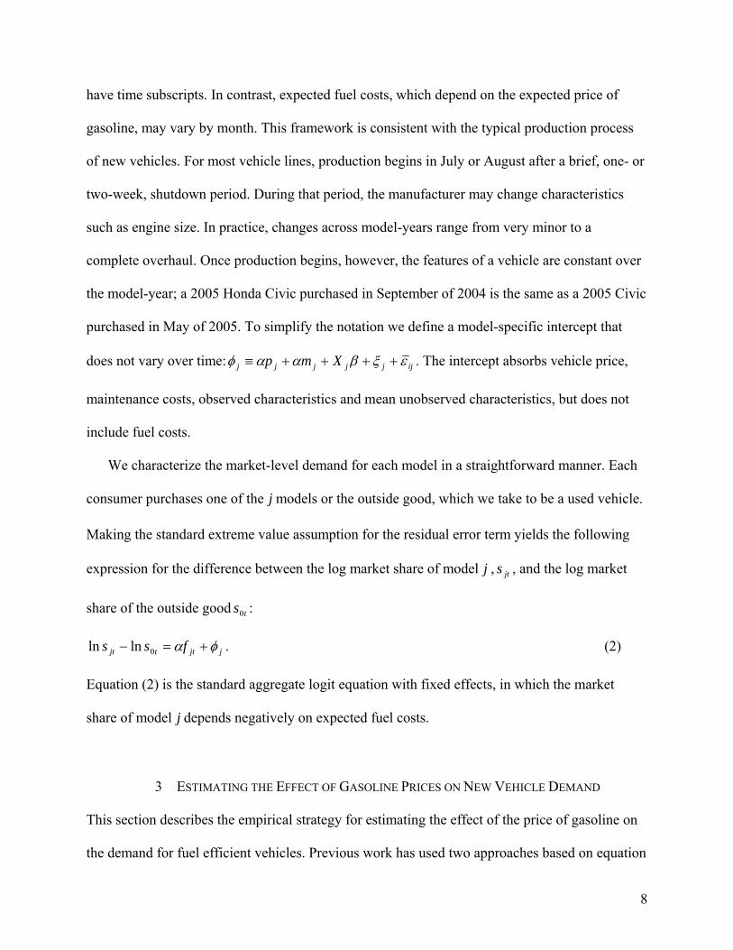
1990s than in other time periods. The MPG distribution is fairly stable, although the share of
models with high fuel efficiency has increased gradually over time, as shown in Figure 3.
The last two rows in Panel A of Table 1 show dollars-per-mile and the log of model sales.
Panel B shows the standard deviations of the dollars-per-mile and sales variables after taking
first differences, which is the transformation used to estimate equation (5) below. Even though
this transformation removes much of the variation, considerable variation remains for both
variables in all four decades.
5 MAIN RESULTS AND IMPLICATIONS FOR MARKET SHARES AND A GASOLINE TAX
5.1 EFFECT OF THE PRICE OF GASOLINE ON VEHICLE DEMAND OVER TIME
Table 2 reports the estimate ofα in equation (5). The dependent variable is the log share of sales
by model and month. The main independent variable is dollars-per-mile, defined as the real price
of gasoline divided by the fuel efficiency of the model, in MPG. The specification includes time
dummies and model-year interactions and the parameters are estimated by Ordinary Least
Squares (OLS). The first row of column 1 of Table 2 reports the estimate ofα , the coefficient on
dollars-per-mile. Standard deviations are in parentheses, clustered by model. The estimate is
-12.64 with standard error 2.52, which is significant at the one percent level.

16
The autocorrelation function of the residuals from this specification indicates significant
serial correlation, however. For that reason, column 2 reports a first differenced specification of
equation (5). The point estimate ofα is similar, -10.45, and is again significant at the one percent
level. All remaining specifications reported in the paper transform the variables by taking first
differences. Serial correlation is further addressed below when lags of the dependent variable are
added.
There are several ways to interpret the magnitude in column 2. First, consider the 2003 Acura
CL (23 MPG) and the 2003 Volkswagen Jetta (32 MPG). The estimate implies that a one dollar
increase in the price of gasoline would reduce sales of the Acura by about 12 percent compared
to sales of the Jetta. The second interpretation of the coefficient is in terms of the elasticity of the
average MPG of new vehicles with respect to the price of gasoline. The estimated elasticity is
about 0.12, which falls between the estimates of Austin and Dinan (2005) and Small and Van
Dender (2007).14
While our primary interest is in explaining the trends shown in Figure 1 and estimating the
effect of the gasoline tax on average fuel efficiency, it is first necessary to address whetherα has
changed over time. If it has, we would restrict the sample to the most recent time period to
answer these questions; alternatively, a longer sample period could increase efficiency. Column
3 separates the sample into three periods: 1970-1985, which includes the two oil shocks, the
imposition of the CAFE standards and the gasoline price decrease in the mid 1980s; 1986-2001,
during which the price of gasoline was nearly constant; and 2002-2007, which includes several
14 Small and Van Dender (2007) and Hughes et al. (2008) provide evidence that the short and long run own price elasticity of gasoline consumption has decreased in magnitude over the past 30 years. The elasticity can be decomposed into three effects: the elasticity of miles travelled with respect to the gasoline price; the price elasticity of the size of the vehicle stock; and the price elasticity of the average fuel efficiency of the stock. The results reported in Small and Van Dender (2007) indicate that the decrease in the own price elasticity of consumption is due to a decrease in the gasoline price elasticity of miles traveled, and not due to a decrease in the elasticity of average fuel efficiency of the vehicle stock. The results in this paper are thus not inconsistent with the previous study.

17
sharp increases in the price of gasoline, comparable in magnitude to the 1970s shocks. Note that
the table reports the interactions of dollars-per-mile with the time period dummies, so each
coefficient can be interpreted as the response during the corresponding period (i.e., there is no
omitted time period). The results suggest that consumer demand responds to the price of gasoline
when the price is high or increasing, in the 1970s and early 1980s and in the most recent period.
The price of gasoline had a negligible effect on sales when prices were stable in the middle
period, which is consistent with casual observation of the new vehicles market. The results are
also similar if dollars-per-mile is interacted with polynomials of a time trend (not reported). 15 In
most of the remaining analysis, because we are interested in understanding recent changes in
market shares and the effect of a future increase in the gasoline tax, we restrict the sample to the
most recent time period (2002-2007). Also note that we return to the possibility of asymmetric
demand responses at the end of Section 5.2.
5.2 SHORT AND LONG RUN EFFECTS OF GASOLINE PRICES
Table 2 shows that monthly gasoline prices have a statistically and economically significant
effect on monthly new vehicle sales. Yet the two issues discussed in the introduction, the
changes in market shares between 2002 and 2007 as well as the potential impact of an increase in
the gasoline tax on overall fuel economy, are related to longer-term effects of gasoline prices on
vehicle sales. This section shows that the short and long run effects of a change in the price of
gasoline are probably fairly similar in magnitude.
15 We have also estimated specifications that separate the first time period into 1970-1978 and 1978-1985. There is a much stronger demand response in the latter sub-period, which we believe is at least partially due to measurement error (recall that MPG is imputed before 1978). In support of this argument, the estimates are smaller for the latter periods if we use the imputed MPG rather than the actual MPG. Because our primary interest is in characterizing consumer demand in the most recent time period, we do not pursue this question further.

18
In principle, the short run effect could be larger or smaller in magnitude than the long run.
On the one hand, if vehicle prices are sticky, the short run quantity effect would be larger. On the
other hand, short-run production constraints or lags in consumers’ demand response could cause
the long run quantity effect to be larger. For example, if prices increase in the short run to clear
the market because of production constraints,α would understate the long run effect of the price
of gasoline on demand.
Column 1 of Table 3 reports the same specification as column 3 of Table 2, except that the
sample is restricted to the model-years 2002-2007. The remainder of the paper refers to this
specification as the baseline. Columns 2-8 in Table 3 report specifications that investigate the
relationship between the short and long run effects. Columns 2-4 add three lags of dollars-per-
mile, three lags of the dependent variable, and 3 lags of both variables. Column 2 shows that the
one-month lag of dollars-per-mile has a moderate, although not statistically significant, effect on
sales, and additional lags are not significant. Column 3 shows that adding lags of the dependent
variable does not affect the estimate on dollars-per-mile, although some of the lags are
statistically significant. The coefficient on the lagged variable implies that a one percent decrease
in last month’s sales is associated with a 16 percent increase in current sales. The negative sign
suggests that a gasoline price shock causes automobile dealers to draw down inventories, after
which vehicle prices respond to partially offset the quantity change. The result is consistent with
Langer and Miller (2008), who find that transaction prices respond to current and lagged
gasoline prices. These estimates can be used to calculate the within-year effect of the price of
gasoline on sales (Small and Van Dender, 2007); based on the estimates for the lag dependent
variables, the within-year response is therefore within about 20 percent of the within-month
19
response. If we consider the within-year effect to constitute the medium run, we conclude that
the short and medium run quantity responses are similar in magnitude.
It is also possible that the effect across years is different from the within-month or within-
year effects. For example, production constraints could explain such long lags – several
automakers have recently announced plans to significantly reduce production of large SUVs over
the next five years. We take two approaches to investigate this possibility. First, we construct a
variable that proxies for the change in consumer demand over the previous year for the vehicle.
The variable is motivated by a model in which firms plan production in August for the following
model-year based on the expected price of gasoline. Consider production planning in August of
year 2−y . If the price follows a random walk, the error in the average expected price over the
following model-year equals the difference between the average price (September to the
following August) and the price in August: 2,1 −− − yAugy pp . The unexpected decrease in average
demand for the vehicle over the model-year is therefore proportional to the ratio of the
expectation error to the fuel efficiency of the vehicle: 1,
2,1
−
−− −
yj
yAugy
MPGpp
; we define this variable as
the lag demand shock. If a firm experiences a decrease in demand for its vehicle over model-
year 1−y , then by the random walk assumption, this decrease should be permanent. Therefore,
the firm will reallocate production in model-year y . If the lag demand shock is added to the
baseline equation, we expect the coefficient on the variable to be negative. Columns 5-8 show
that the main results are not affected much by adding this variable to the specifications in
columns 1-4. The coefficient on the lag demand shock is negative in the lag dependent variable
specifications, but the magnitude is much smaller thanα . There is thus some evidence that firms

20
re-allocate production across years in response to unexpected changes in the price of gasoline,
but the average effect is not quantitatively large.
The second approach to investigating the long run response is to use model dummies instead
of model-year interactions in equation (5) and include additional lags of dollars-per-mile. If 36
lags are added to equation (5), the coefficient on current dollars-per-mile is similar to the
baseline specification. Although there is some evidence for a lagged effect of up to two years, the
magnitudes are relatively small. The results are not reported due to space considerations, but are
available upon request.
Table 2 showed that the effect of the price of gasoline on sales has varied over time. This
pattern raises the possibility that the relationship between gasoline prices and sales is nonlinear
or asymmetric. In the baseline specification in column 1 of Table 3,α is the average effect of
dollars-per-mile on log market share. If the effect is greater at high gasoline prices, or differs in
magnitude for price increases and decreases, the estimates would lead to incorrect conclusions
about the causes of recent changes in market shares or the effect of a gasoline tax. Column 9
adds to the baseline equation the interaction of dollars-per-mile with a dummy variable that is
equal to one if the price of gasoline increased between the previous and current month (the time
dummies absorb the main effect of the dummy variable). The effect of a price increase on sales
would be larger than a decrease if the interaction were negative, but the results indicate that the
response is roughly symmetric. We have investigated other specifications that allow for
nonlinear or asymmetric responses, such as following Dargay and Gately (1997) by
decomposing price changes into three series: the maximum price up until the current month, a
non-decreasing series of price increases and a non-increasing series of price cuts.16 The
16 More precisely, the price increase series equals the cumulative sum of price decreases since the first month in the sample, where a price increase at time t is the difference between the price at time t and the price at time 1−t if the

21
specification distinguishes between rising and falling prices and between short and long-term
changes. The results in column 10 do not provide evidence that demand responds asymmetrically
or in a non-linear fashion, as the coefficients on the three variables are statistically
indistinguishable. Overall, we find the estimate ofα reported in column 1 of Table 3 to be close
to several different estimations of what we consider to be the long run effect of the price of
gasoline on new vehicle demand. While this result is perhaps somewhat surprising, the upshot is
that we can use the empirical approach to address the two main questions: the cause of recent
changes in market shares and the effect of the gasoline tax on average fuel efficiency.17
5.3 EFFECT OF GASOLINE PRICES ON MARKET SHARES OF U.S. FIRMS AND SUVS
Between August of 2002 and August of 2007 the real price of gasoline increased from $1.75 to
$2.86 per gallon. During the same time period, the market share of small SUVs increased from
7.5 to 10.5 percent, while the market share of large SUVs decreased from 18.3 to 10.5 percent.
At the same time, market shares of U.S. manufacturers, which rely on sales of large vehicles,
have declined by 20 percent. It is unclear, though, how much of these changes have been caused
by gasoline prices.
Our identification strategy allows us to determine how much of the recent changes in market
shares are caused by the increase in the price of gasoline. We assume that within-year changes in
gasoline prices are uncorrelated with within-year changes in preferences, i.e., that the model-year
intercepts absorb changes in preferences. This assumption is valid if preferences are slow-
price at time t is greater, and zero otherwise. The price decrease series is defined analogously as the sum of price decreases. 17 We have also estimated specifications that aggregate monthly sales and gasoline prices to quarterly sales and prices. If the long run response were different in magnitude than the monthly response, the quarterly results would likely be different. The estimates are available upon request, and are similar to the baseline.

22
moving and within-year preference shocks are uncorrelated with the price of gasoline, which
seems likely to be the case; Section 6.2 provides some empirical support for this assumption. We
estimate the effect of the price increase on SUV market shares by computing the counterfactual
market shares if the price had remained constant at the 2002 level. We then compare the actual
and counterfactual SUV market shares to determine the effect of gasoline prices on large SUV
demand, and similarly for small SUVs.18 The estimate ofα in column 1 of Table 3 implies that
the increase of $1.11 per gallon caused about 25 percent of the decrease in the market share of
large SUVs and the increase in the market share of small SUVs.19
Turning to U.S. firms, about 40 percent of the decrease in U.S. market share has been caused
by the recent increase in the price of gasoline. We conclude that the price of gasoline has a
substantial effect on the new vehicles market, although perhaps smaller than some recent
analysts have suggested.
5.4 EFFECT OF A GASOLINE TAX ON AVERAGE FUEL EFFICIENCY
We now relate our model to the economic policy issue of reducing gasoline consumption. The
policy debate has focused on raising the CAFE standard, a command-and-control type regulation
that applies to new vehicles sold. Many economists, however, have argued that raising the
gasoline tax instead would be more efficient. The welfare comparison of the two policies
depends partly on the sensitivity of new vehicle demand to the price of gasoline (Austin and
Dinan, 2005). Equation (5) estimates precisely this effect.
18 The negative estimate ofα implies that all market shares decrease when the price of gasoline increases. It is therefore necessary to renormalize the market shares to sum to one when comparing the actual and counterfactual SUV market shares. A similar renormalization is made in the following discussion of the gasoline tax. 19 These results do not appear to be sensitive to the functional form assumptions in equation (5), as the results are similar if a separateα is estimated for each model-year.

23
We use the estimate ofα to calculate the change in average fuel efficiency of new vehicles
due to a one dollar increase in the price of gasoline. The calculation is based on the predicted
market shares of models for which sales are positive at the end of the sample period. The first
column of Table 4 reports the difference between the predicted and actual sales-weighted MPG
for the baseline specification in column 1 of Table 3. The standard error is reported in
parentheses, calculated using the delta method.20 The estimate ofα implies that a one dollar price
increase would raise average fuel efficiency by 1.08 MPG, which is significant at the one percent
level. As noted above, the elasticity of average fuel efficiency with respect to the price of
gasoline is therefore about 0.12, which is roughly one-half of that reported by Austin and Dinan.
6 ROBUSTNESS CHECKS
6.1 ALTERNATIVE ESTIMATION MODELS
As noted above, equation (5) includes several functional form assumptions. Columns 2-4 of
Table 4 report the estimated effect of a one dollar price increase on average fuel efficiency using
a number of different estimation models that relax the main assumptions in equation (5).
Equation (5) was derived by assuming that dollars-per-mile has the same effect on every
consumer’s utility. By comparison, random coefficients logit models, such as BLP, allow for a
separate iα for each consumer. In that case, the effect of dollars-per-mile on the market share of a
particular model is the average iα , weighted by the probability individuals purchase the specific
model. Consequently, there is a separate jα for each model. Researchers commonly assume that
jα is normally distributed and estimate the mean and standard deviation of the distribution. Our
20 We assume that actual market shares are measured without error, and that the only uncertainty arises from sampling variation overα . The standard errors are computed by taking the first order approximation of the mean market share, which is a nonlinear function ofα .

24
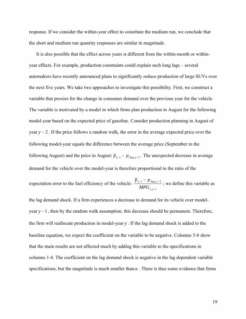
data include sufficient observations to simply estimate a separate jyα for each model-year in
equation (5) using observations from 2002-2007. Figure 4 plots a histogram of the estimated
coefficients, which indicates that there is some heterogeneity, but that most coefficients fall
within a fairly narrow interval, between -5 and -30. Column 2 in Table 4 uses the estimated
coefficients from this specification to calculate that a one dollar price increase raises average fuel
efficiency by 1.20 MPG, which is quite similar to the baseline in column 1 and is significant at
the 5 percent level.
We next estimate a model based loosely on the Almost Ideal Demand System (AIDS) of
Deaton and Muellbauer (1980), which gives an arbitrary first order approximation to any set of
demand equations. In the standard AIDS model, the dependent variable is the model’s share of
revenue in total market revenue and the independent variables are the prices of all models. But in
the current setting, the total cost of purchasing and using a model is the sum of the vehicle’s
price and operating costs. As in equation (5), including model-year intercepts absorbs the
vehicle’s price and maintenance costs, leaving the following equation:
jtjytjg
tjjt QPw υφλγ +++= ˆlnln , (6)
where the dependent variable is the revenue share of the model calculated using annual retail
prices. The first independent variable is the log price of gasoline; the second independent
variable is aggregate sales, using the approximation in Deaton and Muellbauer; jyφ is a model-
year fixed effect and jtυ is an error term. The coefficient jγ is the effect of a one percent increase
in the price of gasoline on the revenue share of model j ; the specification allows the price of
gasoline to affect the revenue share of each model differently. The second independent variable
controls for the relationship between total sales and the revenue share of each model, and the
coefficient can also vary freely across models. We estimate equation (6) by taking first

25
differences of all variables using observations from 2002-2007. Figure 5a shows a histogram of
the jγ coefficients and Figure 5b plots the coefficients against the MPG of the corresponding
model. Figure 5b shows a strong positive correlation, indicated by the fitted line, which suggests
that an increase in the price of gasoline causes the relative revenue shares of fuel efficient
vehicles to increase. Column 3 of Table 5 confirms this result, using the predicted change in
market shares to calculate the change in average MPG caused by a one dollar gasoline price
increase. The estimate is 0.79 MPG, which is somewhat smaller than the other estimates. The
estimate is not statistically significant, which is not surprising given the large number of
estimated coefficients.
Finally, instead of making assumptions on consumer preferences and the distributions of
unobserved parameters, we can estimate an aggregate regression that characterizes the effect of
the price of gasoline on average fuel efficiency:
tymg
tt PMPG ωτμδ +++= lnln (7)
The dependent variable is the log of the monthly sales-weighted average MPG of new vehicles
and the first independent variable is the log monthly price of gasoline. The regression includes
month and year dummies and the coefficientδ is the elasticity of average MPG to the price of
gasoline. The advantage of this specification is thatδ is simple to interpret, as a linear
approximation to the effect of the gasoline price on average MPG. On the other hand, the
equation cannot be derived from a model of consumer behavior and the results cannot be used to
answer questions pertaining to the effect of gasoline prices on market shares of U.S.
manufacturers and SUVs. Nevertheless, equation (7) is estimated for comparison using
observations from 2002-2007. The estimate of δ is 0.063 with standard error 0.015, which is
significant at the one percent level, implying that a one percent increase in the price of gasoline

26
raises average fuel efficiency by 0.06 percent. Column 4 of Table 4 reports that a one dollar
increase in the price of gasoline raises average fuel efficiency by 0.50 MPG, which is smaller
than the other estimates, but which has similar implications for the effect of the gasoline tax.
6.2 ADDITIONAL SPECIFICATIONS
The preceding sections have documented a strong relationship between the price of gasoline and
the demand for fuel efficient vehicles. Next we utilize alternative vehicle characteristics. Models
with greater fuel efficiency are generally smaller and lighter, so an increase in the price of
gasoline should also lead to larger market shares of small and light models. Columns 1-4 of
Table 5 show that this is the case, which provides further support for the main results.
We consider four characteristics: weight, length, engine size and number of cylinders. The
fact that driving costs should affect consumer decisions similarly to model prices motivated the
use of dollars-per-mile when analyzing fuel efficiency, but there are no corresponding theoretical
arguments to guide the functional forms for the other characteristics. Instead, we use a semi-
parametric approach and separate models into quartiles for weight, length and engine size, as
well as three categories for engines with 4, 6 or 8 cylinders. Columns 1-4 report estimates of
equation (5), replacing dollars-per-mile with the interactions of the log price of gasoline with the
quartile or cylinder indicator variables. Models that are light, short or have small engines
constitute the first and omitted categories in the four columns. The results consistently show that
an increase in the price of gasoline causes a decrease in the market shares of large, heavy models
that have large engines.
In the baseline specification we assume that dollars-per-mile is exogenous to other time-
varying determinants of sales, such as transaction prices. As noted earlier, the price of gasoline

27
could affect transaction prices, which was investigated using a reduced form approach in Table
3. However, the price of gasoline may be correlated with transaction prices or other unobserved
variables and therefore would not be truly exogenous. We next investigate bias arising from two
potential omitted variables, and conclude that the empirical strategy appears to be robust.
Previous work, e.g., Copeland et al. (2005) has found that transaction prices vary
differentially within the model-year for different market segments and sizes. Column 5 controls
for this pattern by including the interaction of a set of month dummy variables with a set of
indicators for the quintile of the model’s fuel efficiency. This specification allows models in each
fuel efficiency quintile to have different transaction price and sales profiles. The estimate is quite
similar to the baseline and suggests that these profiles are uncorrelated with dollars-per-mile.21
Another possible source of bias is that the price of gasoline may be correlated with the
composition of consumers that purchase vehicles. Sufficiently detailed and high frequency data
are not available to investigate this possibility directly, but we can address this concern by
adding calendar month-vehicle market segment interactions to the baseline specification. The
specification controls for seasonal patterns of demand. For example, if the price of gasoline
happens to increase during winter months in the sample and SUV consumers are less likely to
purchase vehicles in the winter, the estimate ofα could reflect a spurious correlation. Column 6
controls for seasonal effects, and shows that the estimate ofα remains robust. The specification
provides support for the assumption that the price of gasoline is uncorrelated with consumer
preferences.
7 CONCLUSION 21 Manufacturer incentives have become increasingly common in the past decade (Busse et al., 2007), particularly among U.S. manufacturers. These incentives do not appear to bias the results, as the estimates are similar if we omit U.S. firms.

28
This paper estimates the effect of the price of gasoline on the demand for fuel efficient vehicles.
The empirical strategy combines time series variation of the price of gasoline with cross
sectional variation of fuel efficiency, exploiting the fact that the effect of a gas price change on
fuel costs is inversely proportional to fuel efficiency. We control for unobserved characteristics
that vary by model-year by using monthly gasoline price and sales data, combined with model-
year fixed effects. The price of gasoline has a significant effect on the demand for fuel efficient
vehicles. Based on specifications including lags and allowing for asymmetries, we find that the
short run quantity response to a price shock is similar to the long run response. The estimates
imply that the increase in the price of gasoline from 2002-2007 explains much of the change in
the market shares of SUVs and of U.S. automakers. Turning to the policy question of using the
gasoline tax to reduce fuel consumption, an increase in the Federal gasoline tax that raises the
price of gasoline by one dollar would raise the average fuel efficiency of new vehicles by about
0.5-1 MPG.
This study, as well as previous empirical work, considers the effect of the price of gasoline
on new vehicle demand, using a static approach in which the set of models is exogenous.
Gasoline prices and regulations such as CAFE may affect the characteristics of vehicles in the
market, including fuel efficiency. Further work should consider a dynamic setting, in which
vehicle characteristics are endogenous.
8 REFERENCES
1. Austin, David and Terry Dinan (2005). “Clearing the Air: The Costs and Consequences of Higher CAFE Standards and Increases in Gasoline Taxes.” Journal of Environmental Economics and Management: vol. 50, 562-582.
2. Bento, Antonio M., Lawrence H. Goulder, Mark R. Jacobsen and Roger H. von Haefen (2006), “Distributional and Efficiency Impacts of Increased U.S. Gasoline Taxes.”

29
3. Berry, Steven, James Levinsohn and Ariel Pakes (1995), “Automobile Prices in Market Equilibrium,” Econometrica: vol. 63(4), 841-890.
4. Boyd, J. Hayden and Robert E. Mellman (1980). “The Effect of Fuel Economy Standards on the U.S. Automotive Market: an Hedonic Demand Analysis.” Transportation Research: vol. 14A, 367-378.
5. Busse, Meghan R., Jorge Silvo-Risso and Florian Zettelmeyer (2005). “‘$1000 Cash Back’: The Pass-Through of Auto Manufacturer Promotions.” American Economic Review, vol 96(4), 1253-70.
6. Busse, Meghan R., Duncan Simester and Florian Zettelmeyer (2007). “‘The Best Price You’ll Ever Get’: The 2005 Employee Discount Pricing Promotions in the U.S. Automobile Industry.”
7. Chouinard, Hayley H. and Jeffrey M. Perloff (2007), "Gasoline Price Differences: Taxes, Pollution Regulations, Mergers, Market Power, and Market Conditions," The B.E. Journal of Economic Analysis & Policy: vol. 7 : Iss. 1 (Contributions), Article 8
8. Copeland, Adam, Wendy Dunn and George Hall (2005), “Prices, Production and Inventories Over the Automotive Model Year.”
9. Copeland, Adam and George Hall (2005), “The Response of Prices, Sales and Output to Temporary Changes in Demand.”
10. Corrado, Carol, Wendy Dunn and Maria Otoo (2006), “Incentives and Prices for Motor Vehicles: What Has Been Happening In Recent Years?”, Finance and Economics Discussion Series, Board of Governors of the Federal Reserve System, 2006-09.
11. Deaton, Angus and John Muellbauer (1980), “An Almost Ideal Demand System,” The American Economic Review: vol. 70, n3, 312-326.
12. Dubin, J. A. and D. L. McFadden (1984), “An Econometric Analysis of Residential Electric Appliance Holdings and Consumption,” Econometrica: vol. 52, n2, 345-362.
13. Ellerman, A. Denny, Henry D. Jacoby and Martin B. Zimmerman (2006). “Bringing Transportation into a Cap-and-Trade Regime.” MIT Joint Program on the Science and Policy of Global Change, Report No. 136, June.
14. Goldberg, Pinelopi Koujianou (1998), “The Effects of the Corporate Average Fuel Efficiency Standards in the US,” The Journal of Industrial Economics: vol. 46, n1, 1-33.
15. Hooker, Mark A. (1996). “What Happened to the Oil Price-Macroeconomy Relationship?” Journal of Monetary Economics, vol. 38, 195-213.
16. Hughes, Jonathan E., Christopher R. Knittel and Daniel Sperling (2008). “Evidence of a Shift in the Short-Run Price Elasticity of Gasoline Demand.” Energy Journal.
17. Jacobsen, Mark (2007). Evaluating Fuel Economy Standards in a Model with Producer and Household Heterogeneity.
18. Knittel, Chris and Victor Stango (2008). “Incompatibility, Product Attributes and Consumer Welfare: Evidence from ATMs.” BE Journal of Economic Analysis and Policy, vol. 8, n1, Article 1.
19. Linn, Joshua (2008). “Energy Prices and the Adoption of Energy-Saving Technology.” The Economic Journal, vol. 118, 1-27.
20. McCarthy, Patrick S. and Richard S. Tay (1998). “New Vehicle Consumption and Fuel Efficiency: A Nested Logit Approach.” Transportation Research: vol. 34E, 39-51.
21. McManus, Walter S. (2005). “The Effects of Higher Gasoline Prices on U.S. Vehicle Sales, Prices and Variable Profit by Segment and Manufacturer Group, 2001 and 2004.”

30
22. Nevo, Aviv (2000), “A Practitioner’s Guide to Estimation of Random-Coefficients Logit Models of Demand,” Journal of Economics and Management Strategy: vol. 9, n4, 513-548.
23. Parry, Ian W. H. and Kenneth A. Small (2005). “Does Britain or the United States Have the Right Gasoline Tax?” The American Economic Review, vol. 95(4), 1276-89.
24. Small, Kenneth and Kurt Van Dender (2007). “Fuel Efficiency and Motor Vehicle Travel: The Declining Rebound Effect.” The Energy Journal, vol. 28, 25-51.
25. Tardiff, Timothy J. (1980). “Vehicle Choice Models: Review of Previous Studies and Directions for Further Research.” Transportation Research: vol. 14A, 327-335.
26. Timiraos, Nick (2007). “The Gasoline Tax: Should it Rise?” The Wall Street Journal, August 18-19, p. A4.
27. Ward’s Automotive Yearbook, 1980-2003, Ward’s Communications 28. Ward’s AutoInfoBank, Ward’s Automotive Group 29. West, Sarah E. (2004) “Distributional Effects of Alternative Vehicle Pollution Control
Policies,” Journal of Public Economics: vol. 88, 735-757.
-0.8
-0.6
-0.4
-0.2
0
0.2
0.4
0.6
0.8
1
4/1/2002 1/26/2003 11/22/2003 9/17/2004 7/14/2005 5/10/2006 3/6/2007
Cha
nge
in L
ogs
Sinc
e 20
02Figure 1: Change in Market Shares of U.S. Firms and SUVs and
Gasoline Price, 2002-2007
4/1/2002 1/26/2003 11/22/2003 9/17/2004 7/14/2005 5/10/2006 3/6/2007Date
U.S. Firms Smal SUVs Large SUVs Price
Notes: U.S. firms include Chrysler, Ford and GM. Small sport utility vehicles (SUVs) include crossover utility vehicles, and large SUVs include all other SUVs. The figure plots the change in the log quarterly average of the real gasoline price and market shares of U.S. firms and SUVs, relative to the first quarter of 2002. The real price of gasoline is computed from the BLS and market shares are computed from Wards Auto. See Section 4 for details on data construction.

1
1.6
2.2
2.8
3.4
4
14
16
18
20
22
24
1/1/1970 6/24/1975 12/14/1980 6/6/1986 11/27/1991 5/19/1997 11/9/2002Date
Figure 2a: Quarterly Average MPG and Gasoline Price, 1970-2007
Average MPG Price (right axis)
Figure 2b: First Differenced Log MPG and Log Price, 1970-2007
-0.3
-0.2
-0.1
0
0.1
0.2
0.3
-0.06
-0.04
-0.02
0
0.02
0.04
0.06
1/1/1970 6/24/1975 12/14/1980 6/6/1986 11/27/1991 5/19/1997 11/9/2002Date
g g g ,
Average MPG Price (right axis)
Notes: Average miles per gallon (MPG) is the sales-weighted average MPG by year and quarter. Figure 2a plots average MPG from 1970-2007, and Figure 2b plots the residual of the log of average MPG, after taking first differences and removing annual means and quarter fixed effects. The real price of gasoline is the price of unleaded gasoline divided by the consumer price index, using the national average gasoline price and the consumer price index (CPI) from the Bureau of Labor Statistics. The CPI is normalized to one for April, 2008. Figure 2a plots the real price of gasoline, in 2008 dollars, and Figure 2b plots the residual of the log real price, constructed similarly to average MPG (see text for details).

0
0.05
0.1
0.15
0.2
0.25
14 16 18 20 22 24 26 28 30 32 34 36 38 44
Shar
e of
Mod
els
Miles Per Gallon
Figure 3: MPG Distribution in 1980 and 2007
1980 2007
Notes: The figure plots a histogram of the fuel efficiency, in MPG, of vehicles in the Wards database in the indicated years. The vertical axis is the share of models with positive sales for the corresponding year. The horizontal axis labels the maximum fuel efficiency of vehicles in the bin.

0
20
40
60
80
100
120
-65 -55 -45 -35 -25 -15 -5 5 15 25 35Coefficient
Figure 4: Histogram of Coefficients on Dollars-per-mile by Model
Notes: Figure 4 reports a histogram of the estimated coefficients from equation (5) with a separate coefficient on dollars-per-mile for each model-year. The sample, dependent variable and other independent variables are the same as in column 1 of Table 3. The histogram shows the number of models for which the estimated coefficient falls within the indicated bin.

0
5
10
15
20
25
30
-0.012 -0.01 -0.008 -0.006 -0.004 -0.002 0 0.002 0.004 0.006 0.008 0.01 0.012
Figure 5a: Histogram of Coefficients from Equation (6)
-0.025
-0.02
-0.015
-0.01
-0.005
0
0.005
0.01
0.015
10 15 20 25 30 35 40 45 50
Figure 5b: Coefficient vs. MPG
Notes: Figure 5a reports a histogram of the estimated coefficients from estimating equation (6) separately by model. The dependent variable is the share of revenue in total revenue by month and year for the particular model. The independent variables are a set of year dummies, the log real price of gasoline and the log of aggregate sales. The histogram shows the number of models for which the estimated coefficient falls within the indicated bin. Figure 5b plots the coefficients against the MPG of the model. The solid line indicates the fitted values of an OLS regression of the coefficient on MPG.

1970-1979 1980-1989 1990-1999 2000-2007
2.32 2.41 1.65 2.23(0.18) (0.59) (0.16) (0.53)
15.91 22.06 21.91 21.50(2.88) (5.04) (4.66) (5.45)
0.15 0.11 0.08 0.11(0.03) (0.04) (0.02) (0.03)
8.95 7.89 7.58 7.69(1.07) (1.57) (1.88) (1.81)
0.0027 0.0031 0.0023 0.0057
Log Sales 0.36 0.37 0.39 0.39
Gasoline Price
Table 1:
Summary Statistics
Notes: Cells in Panel A report means with standard deviations in parentheses. The first row of Panel A reports the monthly real gasoline price, computed as in Figure 2. The second row reports the average MPG of all models sold in the indicated decade. The third row reports dollars-per-mile, defined as the ratio of the price of gasoline to MPG. The fourth row reports log monthly sales by model. Panel B reports the standard deviation of the indicated variables after first differencing by model-year.
MPG
Log Sales
Dollars-Per-Mile
Panel A: Sample Means and Standard Deviations
Panel B: Standard Deviations After First Differencing
Dollars-Per-Mile

(1) (2) (3)
-12.64 -10.45(2.52) (1.78)
-10.10(3.48)
-1.50(2.93)
-15.28(2.58)
Number of Observations 76,049 69,089 70,855
R2 0.94 0.02 0.02
First Differences? No Yes Yes
Table 2:
Effect of the Price of Gasoline on New Vehicle Sales, 1970-2007
Dollars-Per-Mile
Dependent Variable: Log Share of Sales
Notes: Standard errors are in parentheses, clustered by model. The table reports the results of estimating equation (5) by Ordinary Least Squares (OLS). The dependent variable is the log share of sales by model and month. All variables are in first differences in columns 2 and 3. All specifications include month dummies and column 1 includes model-year interactions. Columns 1 and 2 report the estimated coefficient on dollars-per-mile, which is constructed as in Table 1. Column 3 reports the interaction of dollars-per-mile with a set of dummy variables, which are equal to one in the indicated years.
Dollars-Per-Mile x 1970-1985
Dollars-Per-Mile x 1986-2001
Dollars-Per-Mile x 2002-2007

(1) (2) (3) (4) (5) (6) (7) (8) (9) (10)
-15.91 -13.98 -17.11 -14.72 -15.39 -13.59 -16.10 -13.96 -18.23(2.54) (4.75) (3.68) (4.44) (2.41) (3.27) (3.85) (4.46) (2.43)
-5.01 -6.48 -5.30 -5.80(4.27) (3.90) (2.64) (4.02)
4.05 2.24 0.22 2.49(4.02) (3.59) (2.89) (3.62)
-0.46 2.05 0.84 2.43(2.82) (2.67) (2.16) (2.69)
-0.16 -0.16 -0.16 -0.16(0.03) (0.03) (0.03) (0.03)
-0.02 -0.02 -0.02 -0.02(0.03) (0.03) (0.03) (0.03)
0.04 0.04 0.03 0.04(0.02) (0.02) (0.02) (0.02)
1.04 1.10 -3.17 -2.77(1.64) (1.63) (2.30) (2.32)
0.35(0.25)
-9.07(8.22)
-9.70(2.54)
-11.44(2.96)
N 15,810 11,493 11,214 11,214 15,189 15,189 10,902 10,902 15,810 68,662
R2 0.02 0.02 0.04 0.04 0.02 0.02 0.04 0.04 0.02 0.02
Price Increase-Per-Mile
Two Month Lag Dollars-Per-Mile
Three Month Lag Dollars-Per-Mile
One Month Lag Dependent Variable
Two Month Lag Dependent Variable
Three Month Lag Dependent Variable
Lag Demand Shock
Price Increase x Dollars-Per-Mile
Max Price-Per-Mile
Price Cut-Per-Mile
Table 3:
Lagged and Asymmetric Demand Responses
One Month Lag Dollars-Per-Mile
Dollars-Per-Mile
Dependent Variable: Log Share of Sales

increases since the beginning of the sample. Column 10 includes the ratio of max price, price cut and price increase to the model's fuel efficiency. See text for details.
Notes to Table 3: Standard errors are in parentheses, clustered by model. The dependent variable is the log share of sales, constructed as in Table 2. Column 1 reports the same specification as column 2 of Table 2, restricting the sample to September, 2002-August, 2007. Columns 2-4 report the same specification as column 1, adding the 1-3 month lags of dollars-per-mile or the 1-3 month lags of the dependent variable. Columns 5-8 repeat the specifications from columns 1-4, adding the lag demand shock variable, defined in the text. Price increase is a dummy variable, equal to one if the current price is greater than the price in the previous month. Column 9 adds to the specification in column 1 the interaction of the price increase with dollars-per-mile. Column 10 uses the full sample, 1970-2007, and replaces dollars-per-mile with three variables defined in Dargay and Gately (1997). Max price is the maximum gasoline price between the beginning of the sample and the current month. Price cut is a non-increasing series, equal to the cumulative sum of price decreases since the beginning of the sample. Price increase is a non-decreasing series, equal to the cumulative sum of price

(1) (2) (3) (4)
1.08 1.20 0.79 0.51(0.19) (0.59) (0.56) (0.12)
Specification Column (1) of Table 3
Column (1), with Separate Coefficient
by Model-YearEquation (6) Equation (7)
Notes: Each column reports the effect of a one dollar increase in the price of gasoline on average MPG. The effects are calculated from the indicated specifications, which use observations from 2002-2007. Column 1 uses the same specification as column 1 of Table 3. Column 2 uses the same specification as column 1, except that a separate coefficient on the dollars-per-mile variable is estimated for each model-year. Column 3 reports the results of estimating equation (6). Column 4 reports the results of estimating equation (7). In columns 1-3, the calculation uses the predicted market shares of models sold in August, 2007, with and without the price increase. The standard error is in parentheses, calculated using the delta method. The effect of the price increase in column 4 is the change in average miles per gallon if the price increases by one dollar, relative to the price in August, 2007.
Table 4:
Effect of a Price Increase on Average Fuel Efficiency for Alternative Specifications
Effect of One Dollar Price Increase on MPG

(1) (2) (3) (4) (5) (6)
-0.44(0.18)
-0.97(0.18)
-0.93(0.16)
-0.76(0.18)
-0.66(0.17)
-1.07(0.17)
-0.73(0.18)
-0.88(0.17)
-1.05(0.17)
-0.75(0.18)
-1.08(0.17)
-14.71 -13.51(2.91) (2.77)
Number of Observations 14,935 14,935 14,935 14,935 15,810 14,993
R2 0.02 0.02 0.02 0.02 0.02 0.03
Dependent Variable: Log Share of Sales
Dollars-Per-Mile
Table 5:
Other Model Characteristics and Controlling for Model-Sales Profiles
Weight Quartile 2 x Log Price
Weight Quartile 3 x Log Price
Weight Quartile 4 x Log Price
Length Quartile 2 x Log Price
Length Quartile 3 x Log Price
Length Quartile 4 x Log Price
Engine Size Quartile 2 x Log Price
Engine Size Quartile 3 x Log Price
Engine Size Quartile 4 x Log Price
6 Cylinder Engine x Log Price
8 Cylinder Engine x Log Price
Notes: Standard errors are in parentheses, clustered by model. The dependent variable is log sales by model and month. The sample is the same as in column 1 of Table 3. For each month and year, models are assigned quartiles based on their curb weight, length (wheelbase) and engine size (liters). The quartile dummies are interacted with the log price of gasoline. Columns 1-3 report the interaction coefficients, where the first quartile is the omitted category. In column 4 models are separated into three categories, depending on the number of cylinders of the engine. The table reports the coefficients on the 6-cylinder and 8-cylinder interactions, where the omitted category has 4 cylinders. Columns 5 and 6 report the same specification as column 1 of Table 3. Column 5 includes calendar month-MPG quintile interactions and column 6 includes calendar month- vehicle class interactions.