the physics of debris flows - william bechtel's...

THE PHYSICS OF DEBRIS FLOWS

Richard M. IversonCascades Volcano ObservatoryU.S. Geological SurveyVancouver, Washington

Abstract. Recent advances in theory and experimen-tation motivate a thorough reassessment of the physicsof debris flows. Analyses of flows of dry, granular solidsand solid-fluid mixtures provide a foundation for a com-prehensive debris flow theory, and experiments providedata that reveal the strengths and limitations of theoret-ical models. Both debris flow materials and dry granularmaterials can sustain shear stresses while remaining stat-ic; both can deform in a slow, tranquil mode character-ized by enduring, frictional grain contacts; and both canflow in a more rapid, agitated mode characterized bybrief, inelastic grain collisions. In debris flows, however,pore fluid that is highly viscous and nearly incompress-ible, composed of water with suspended silt and clay, canstrongly mediate intergranular friction and collisions.Grain friction, grain collisions, and viscous fluid flowmay transfer significant momentum simultaneously.Both the vibrational kinetic energy of solid grains (mea-sured by a quantity termed the granular temperature)and the pressure of the intervening pore fluid facilitatemotion of grains past one another, thereby enhancingdebris flow mobility. Granular temperature arises fromconversion of flow translational energy to grain vibra-tional energy, a process that depends on shear rates,grain properties, boundary conditions, and the ambientfluid viscosity and pressure. Pore fluid pressures thatexceed static equilibrium pressures result from local orglobal debris contraction. Like larger, natural debrisflows, experimental debris flows of ;10 m3 of poorly

sorted, water-saturated sediment invariably move as anunsteady surge or series of surges. Measurements at thebase of experimental flows show that coarse-grainedsurge fronts have little or no pore fluid pressure. Incontrast, finer-grained, thoroughly saturated debris be-hind surge fronts is nearly liquefied by high pore pres-sure, which persists owing to the great compressibilityand moderate permeability of the debris. Realistic mod-els of debris flows therefore require equations that sim-ulate inertial motion of surges in which high-resistancefronts dominated by solid forces impede the motion oflow-resistance tails more strongly influenced by fluidforces. Furthermore, because debris flows characteristi-cally originate as nearly rigid sediment masses, trans-form at least partly to liquefied flows, and then trans-form again to nearly rigid deposits, acceptable modelsmust simulate an evolution of material behavior withoutinvoking preternatural changes in material properties. Asimple model that satisfies most of these criteria usesdepth-averaged equations of motion patterned afterthose of the Savage-Hutter theory for gravity-driven flowof dry granular masses but generalized to include theeffects of viscous pore fluid with varying pressure. Theseequations can describe a spectrum of debris flow behav-iors intermediate between those of wet rock avalanchesand sediment-laden water floods. With appropriate porepressure distributions the equations yield numerical so-lutions that successfully predict unsteady, nonuniformmotion of experimental debris flows.

1. INTRODUCTION

Debris flows occur when masses of poorly sortedsediment, agitated and saturated with water, surge downslopes in response to gravitational attraction. Both solidand fluid forces vitally influence the motion, distinguish-ing debris flows from related phenomena such as rockavalanches and sediment-laden water floods. Whereassolid grain forces dominate the physics of avalanches,and fluid forces dominate the physics of floods, solid andfluid forces must act in concert to produce a debris flow.Other criteria for defining debris flows emphasize sedi-ment concentrations, grain size distributions, flow frontspeeds, shear strengths, and shear rates [e.g., Beverageand Culbertson, 1964; Varnes, 1978; Pierson and Costa,

1987], but the necessity of interacting solid and fluidforces makes a broader, more mechanistic distinction.By this rationale, many events identified as debris slides,debris torrents, debris floods, mudflows, mudslides,mudspates, hyperconcentrated flows, and lahars may beregarded as debris flows [cf. Johnson, 1984]. The diversenomenclature reflects the diverse origins, compositions,and appearances of debris flows, from quiescentlystreaming, sand-rich slurries to tumultuous surges ofboulders and mud.

Interaction of solid and fluid forces not only distin-guishes debris flows physically but also gives themunique destructive power. Like avalanches of solids,debris flows can occur with little warning as a conse-quence of slope failure in continental and seafloor en-

This paper is not subject to U.S. copyright. Reviews of Geophysics, 35, 3 / August 1997pages 245–296

Published in 1997 by the American Geophysical Union. Paper number 97RG00426● 245 ●

vironments, and they can exert great impulsive loads onobjects they encounter. Like water floods, debris flowsare fluid enough to travel long distances in channels withmodest slopes and to inundate vast areas. Large debrisflows can exceed 109 m3 in volume and release morethan 1016 J of potential energy, but even commonplaceflows of ;103 m3 can denude vegetation, clog drainage-ways, damage structures, and endanger humans (Figure 1).

The capricious timing and magnitude of debris flowshamper collection of detailed data. Scientific under-standing has thus been gleaned mostly from qualitativefield observations and highly idealized, first-generationexperiments and models. However, a new generation ofexperiments and models has begun to yield improvedinsight by simulating debris flows’ key common at-tributes. For example, all debris flows involve gravity-driven motion of a finite but possibly changing mass ofpoorly sorted, water-saturated sediment that deformsirreversibly and maintains a free surface. Flow is un-steady and nonuniform, and is seldom sustained formore than 104 s. Peak flow speeds can surpass 10 m/s andare characteristically so great that bulk inertial forces areimportant. Total sediment concentrations differ littlefrom those of static, unconsolidated sediment massesand typically exceed 50% by volume. Indeed, most de-bris flows mobilize from static, nearly rigid masses ofsediment, laden with water and poised on slopes. Whenmass movement occurs, the sediment-water mixtures

transform to a flowing, liquid-like state, but eventuallythey transform back to nearly rigid deposits. New modelsand measurements that clarify the physical basis of de-bris flow behavior from mobilization to deposition arethe focus of this paper.

Including this introduction, the paper has 10 sections.Section 2 describes the net energetics of debris flowmotion, the variability of debris flow mass, and thechallenges these phenomena pose for researchers. Insection 3 a compilation of key observations, data, andconcepts summarizes qualitatively the factors that con-trol debris flows’ mass, momentum, and energy content.In section 4, scaling analyses assist identification andclassification of debris flow behavior on the basis ofdimensionless parameters that distinguish dominantmodes of momentum transport in solid-fluid mixtures.In section 5 a retrospective of traditional, one-phasemodels for momentum transport in debris flows explainswhy such models are incompatible with current under-standing. In section 6, mass, momentum, and energyconservation equations for two-phase debris-flow mix-tures establish a theoretical framework that highlightsthe variable composition of debris flows and the impor-tance of solid-fluid interactions. In section 7 a relativelycomplete analysis of an idealized debris-flow mixturemoving steadily along a rough bed helps clarify thecomplicated interplay between local solid and fluid mo-tion, boundary forces, and mechanisms of energy dissi-

Figure 1. Digitally enhanced photographs of the path of the 2300 m3 Oddstad debris flow, which occurredJanuary 4, 1982, in Pacifica, California. The flow destroyed two homes and killed three people. The sourcearea slopes 268. The flow path slopes 218 on average and extends 170 m downslope. Deposits at the base ofthe flow path have been removed [Schlemon et al., 1987; Wieczorek et al., 1988; Howard et al., 1988]. (Modifiedfrom USGS [1995], courtesy of S. Ellen and R. Mark.)

246 ● Iverson: PHYSICS OF DEBRIS FLOWS 35, 3 / REVIEWS OF GEOPHYSICS

pation and momentum transport. In section 8 a lesscomplete analysis of unsteady debris flow motion focuseson persistence of nonequilibrium fluid pressures thatdiffer with proximity to debris flow surge fronts. Insection 9, numerical calculations using a simplified,depth-averaged routing model that emphasizes the ef-fects of Coulomb grain friction mediated by persistentnonequilibrium fluid pressures indicate that the modelcan predict the velocities and depths of experimentaldebris flows. Section 10 summarizes the strengths andlimitations of current understanding and suggests prior-ities for future research. Appendices A–C provide somekey mathematical details omitted in previous sections,and a complete summary of mathematical notation fol-lows in a separate notation section.

Because this paper emphasizes physical aspects ofdebris flow motion, it includes only incidental coverageof important topics such as debris flow habitats, frequen-cies, magnitudes, triggering mechanisms, hazard assess-ments, engineering countermeasures, morphology andsedimentology of debris flow deposits, and the relation-ship between debris flows and other mass movements.Several previous reviews and compilations, such as thoseby Takahashi [1981, 1991, 1994], Innes [1983], Costa[1984], Johnson [1984], Costa and Wieczorek [1987],Hooke [1987], Pierson [1995], and Iverson et al. [1997]treat these subjects more completely. In addition, video-tape recordings [Costa and Williams, 1984; Sabo PublicityCenter, 1988] reveal many qualitative attributes of debrisflows, and summaries by Iverson and Denlinger [1987],Miyamoto and Egashira [1993], Savage [1993], and Hutteret al. [1996] introduce some of the quantitative conceptselaborated here.

2. BULK ENERGETICS AND RUNOUT EFFICIENCY

The energetics of debris flows differ dramaticallyfrom those of a homogeneous solid or fluid. The inter-actions, and not merely the additive effects of the solidand fluid constituents, are important. A simple thoughtexperiment helps illustrate this phenomenon:

Consider first a very unrealistic but simple model of adebris flow. A mass of identical, dense, frictionless elas-tic spheres flows down a bumpy, rigid incline and onto ahorizontal runout surface, all within a vacuum. Thespheres jostle and collide as they accelerate downslope,but no energy dissipation occurs, and the flow runs outforever. Then fill the spaces between the spheres with aviscous fluid less dense than the spheres (e.g., liquidwater), and repeat the experiment. Owing to viscousshearing, the mixture loses energy as it moves down-slope, and runout remains finite. The fluid retards themotion. Next, replace the elastic spheres with rough,inelastic sediment grains, and repeat the two experi-ments. In the vacuum the collection of grains runs out afinite distance and stops owing to energy dissipationcaused by grain contact friction and inelastic collisions.

What is the outcome of the experiment when the inter-stices between the sediment grains are filled with viscousfluid? A logical possibility, suggested by the behavior ofelastic spheres, is that the viscous fluid will increasedissipation and reduce runout. However, experiencewith water-saturated debris flows shows that the pres-ence of viscous fluid increases runout even though thefluid dissipates energy. Interactions of viscous fluid withdissipative solid grains of widely varying sizes producethis behavior and merit emphasis in efforts to under-stand debris flow motion.

As the preceding thought experiment implies, debrisflow motion involves a cascade of energy that begins withincipient slope movement and ends with deposition. Asa debris flow moves downslope, its energy degrades tohigher entropy states and undergoes the following con-versions:

bulk gravitational potential energy

3 bulk translational kinetic energy

º grain vibrational kinetic energy

1 fluid pressure energy3 heat

Here right pointing arrows denote conversions that areirreversible, except in special circumstances, whereas thetwo-way arrow denotes a conversion that apparentlyinvolves significant positive feedback. The details of thisenergy cascade encompass virtually all the importantissues of debris flow physics. Before pursuing these de-tails, however, it is worthwhile to consider debris flowenergetics from a broader perspective.

The net efficiency of debris flows, and of kindredphenomena such as rock and snow avalanches, describesconversion of gravitational potential energy to the workdone during debris flow translation. The more efficientlythis conversion occurs, the less vigorously energy de-grades to irrecoverable forms such as heat, and thefarther the flow runs out before stopping. Net efficiencycan be evaluated by integrating an equation that de-scribes motion of the debris flow center of mass as afunction of time. Alternatively, as was recognized origi-nally by Heim [1932] for rock avalanches, the outcome ofthe integration can be obtained without specifying anequation of motion by equating the total potential en-ergy lost during motion, MgH, to the total energy de-graded to irrecoverable forms by resisting forces, MgR,that work through the distance L to make the debris flowstop:

MgH 5 MgRL (1)

Here M is the debris flow mass, g is the magnitude ofgravitational acceleration, and R is a dimensionless netresistance coefficient, which incorporates the effects ofinternal forces but which depends also on external forcesthat act at the bed to convert gravitational potential tohorizontal translation. The coordinates H and L de-

35, 3 / REVIEWS OF GEOPHYSICS Iverson: PHYSICS OF DEBRIS FLOWS ● 247

scribe displacement of the debris flow center of massduring motion: H is the vertical elevation of the debrisflow source above the deposit, and L is the horizontaldistance from source to deposit (Figure 2).

Even though all debris flow energy ultimately de-grades to heat, thermodynamic data provide few con-straints for evaluating R in (1). The equation shows thata debris flow’s total energy dissipation per unit mass isgiven by gH, which implies about 10 J/kg of heat pro-duction per meter of flow descent. Even without heatloss, this 10 J/kg suffices to raise the temperature of atypical debris flow mixture only about 0.0058C. Conse-quently, debris flow temperature measurements in open,outdoor environments, with unrestricted heat exchangeand ambient temperatures that vary widely, yield littleresolution of energy dissipation due to flow resistance.Instead, debris flow physics conventionally emphasizesthe purely mechanical behavior of an isothermal system,and this paper follows that convention.

The mechanical phenomena that govern R must bequantified in detail to understand and predict debrisflow motion, but evaluation of net efficiency from theaftermath of a debris flow is far simpler. Dividing eachside of (1) by MgHR yields

1/R 5 L/H (2)

which shows that the net efficiency, defined as 1/R,increases as the runout distance L increases for a fixeddescent height, H. Thus net efficiency may be deter-mined from surveys of debris flow source areas anddeposits that yield the value of L/H.

Rigorous evaluations of L/H from debris flows’ cen-ter-of-mass displacements have been rare, but field map-ping of debris flow paths and detailed measurements onexperimental debris flows demonstrate three importantpoints [cf. Vallance and Scott, 1997]: (1) L/H of water-saturated debris flows exceeds that of drier sedimentflows with comparable masses, (2) Large debris flowsappear to have greater efficiency than small flows, and(3) L/H depends on runout path geometry and boundaryconditions that determine, for example, the extent oferosion, sedimentation, and flow channelization. Table 1

summarizes typical L/H values inferred from the distallimits of debris flow source areas and deposits. Thetabulated L/H values can be compared in only thebroadest sense because the data were collected on debrisflows with diverse origins and flow path geometries byinvestigators with diverse objectives. Nonetheless, thedata of Table 1 indicate that L/H increases roughly inproportion to the logarithm of volume for debris flowswith volumes greater than about 105 m3 but that L/Hremains fixed at ;2–4 for smaller flows. Data for dryrock avalanches exhibit similar trends but indicate thatdry avalanches typically have only about half the effi-ciency (L/H) of debris flows of comparable volume [cf.Scheidegger, 1973; Hsu, 1975; Davies, 1982; Li, 1983;Siebert, 1984; Hayashi and Self, 1992; Pierson, 1995].These empirical trends are noteworthy, but case-by-casevariations in debris-flow behavior make runout predic-tion on the basis of only L/H rather questionable.

Rigorous evaluation of L/H from center-of-mass dis-placements under controlled initial and boundary con-ditions has been possible at the U.S. Geological Survey(USGS) debris flow flume (Figure 3) [Iverson andLaHusen, 1993]. Experiments in which about 10 m3 of awater-saturated, poorly sorted, sand-gravel debris flowmixture is suddenly released from a gate at the head ofthe flume yield L/H ; 2 for unconfined runout butL/H . 2 for channelized runout (Figure 4). Thesevalues surpass the L/H for runout of similar sand-gravelmasses not saturated with water [Major, 1996]. When thesand-gravel mix is replaced by well-sorted gravel, how-ever, the influence of water on the outcome of experi-ments changes: dry gravel produces L/H . 2, but water-saturated gravel produces L/H , 2. Thus waterenhances the mobility of poorly sorted debris flow sed-iments in a manner not manifested by mixtures of well-sorted gravel and water, and experiments with water-gravelmixtures provide a poor surrogate for experiments withrealistic debris-flow materials.

Effects of water-sediment interactions pose challeng-ing problems that consume much of the remainder ofthis paper, but effects of debris flow mass are even moreenigmatic. According to equations (1) and (2), debrisflow mass should not affect runout efficiency, but thedata of Table 1 contradict this inference. The cause ofthis contradiction is difficult to resolve because debrisflows and avalanches can change their mass and compo-sition while in motion and can spread longitudinally tochange their mass distribution [cf. Davies, 1982]. Somedebris flows grow severalfold in mass owing to bed andbank erosion [Pierson et al., 1990] and others declinesubstantially in solids concentration as a result of mixingwith stream water [Pierson and Scott, 1985]. Changes indebris flow mass or composition have been identifiedsomewhat interchangeably by the terms “bulking” (in-crease of mass or solids concentration) and “debulking”(decrease of mass or solids concentration), but moreprecise terminology is desirable because changes in de-

Figure 2. Schematic cross section defining H and L for debrisflow paths. Strictly, H and L are defined by lines that connectthe source area center of mass and the deposit center of mass.In practice, H and L are commonly estimated from the distallimits of the source area and deposit.


bris-flow mass, independent of changes in composition,might influence efficiency.

Attempts to use elementary energy balances to pre-dict effects of mass change on debris flow efficiencyencounter difficulties, which can be traced to assump-tions implicit in equation (1) and in similarly simplemomentum balances [cf. Cannon and Savage, 1988;Hungr, 1990; Erlichson, 1991]. It might seem from (1),for example, that loss of mass during motion shouldincrease efficiency because the potential energy initiallyavailable to power the motion, MgH, stays fixed, whilethe work done by resisting forces apparently declines asthe flow mass declines. The problem with this logic liesin the assumption that R remains constant or decreasesas the flow mass declines. This assumption would becorrect if R depended only on internal forces, but Rdepends also on the external forces that cause the flowmass to decline. Loss of debris flow mass requires thatwork be done on the flow by the banks and bed todecelerate and deposit the lost mass. This work adds tothe work that would be done over the same path lengthin the absence of deposition. The critical question iswhether the additional work is less than the energysavings accrued by leaving mass behind. Universal an-swers to this question are perhaps unattainable. Thesame is true for the question of whether mass gain willincrease bulk mobility and runout. In each case, masschange depends on work done during momentum ex-

change with the bed and banks, which may differ greatlyin different localities. Despite the lack of clear resolu-tion, recognition of the fundamental effects of externalforces on debris flow efficiency is essential, for otherwiseit may be tempting to attribute differences in runoutsolely to differences in flow composition and rheology.Section 7 delves more deeply into the mechanical effectsof external forces.

3. MASS, MOMENTUM, AND ENERGY CONTENT:DESCRIPTION AND DATA

An empirical picture of debris flow physics can bedrawn from a combination of real-time field observa-tions and measurements [e.g., Okuda et al., 1980; Li andYuan, 1983; Johnson, 1984; Pierson, 1980, 1986], detailedobservations and measurements during controlled fieldand laboratory experiments [e.g., Takahashi, 1991; Khe-gai et al., 1992; Iverson and LaHusen, 1989, 1993], andanalyses of debris flow paths and deposits [e.g., Fink etal., 1981; Pierson, 1985, 1995; Whipple and Dunne, 1992;Major, 1996]. Furthermore, videotape compilations ofdebris flow recordings provide many qualitative insights[Costa and Williams, 1984; Sabo Publicity Center, 1988].Relatively little detailed information is available for sub-aqueous debris flows, but most aspects of their behavior(other than their tendency to hydroplane, entrain sur-

TABLE 1. Estimated Values of Total Flow Volume, Runout Distance L, Descent Height H, and Efficiency L/Hof Various Debris Flows

Flow Location Date Reference

FlowVolume,

m3 L, m H, m L/H Origin

Mount Rainier, Osceolamudflow

circa 5700 B.P. Vallance and Scott[1997]

;109 120,000 4,800 25 landslide and down-stream erosion

Nevados Huascaran, Peru May 31, 1970 Plafker and Ericksen[1978]

;108 120,000 6,000 20 landslide

Nevado del Ruiz, Colombia,Rıo Guali

Nov. 13, 1985 Pierson et al.[1990]

;107 103,000 5,190 20 pyroclasts meltingsnow

Mount St. Helens, SouthFork Toutle

May 18, 1980 Fairchild and Wigmosta[1983]

;107 44,000 2,350 19 wet pyroclasticsurge

Mount St. Helens, MuddyRiver

May 18, 1980 Pierson [1985] ;107 31,000 2,150 14 wet pyroclasticsurge

Wrightwood, Calif., Heath Canyon May 7, 1941 Sharp and Nobles[1953]

;106 24,140 1,524 16 landslide

Three Sisters, Oreg., SeparationCreek

1933 J. E. O’Connor et al.(manuscript inpreparation, 1997)

;106 6,000 700 9 glacier breakoutflood

Mount Thomas, NZ, Bullock Creek April 1978 Pierson [1980] ;105 3,500 600 6 landslideWrightwood, Calif., Heath Canyon May 1969 Morton and Campbell

[1974];105 2,700 680 4 landslide

Santa Cruz, Calif., WhitehouseCreek

Jan. 4, 1982 Wieczorek et al. [1988] ;105 600 200 3 landslide

Pacifica, Calif., Oddstad site Jan. 4, 1982 Howard et al. [1988] ;103 190 88 2 landslideUSGS debris flow flume Sept. 25, 1992 Iverson and LaHusen

[1993];101 78 41 2 artificial release

from flume gate

Most data are for flows that were observed during motion or within hours of deposition. With the exception of the Osceola mudflow, all flowsapparently maintained a relatively constant mass (within a factor of 2) from initiation to deposition. The Osceola is included in the tabulationbecause it is the largest well-documented debris flow in the terrestrial geologic record.


rounding water, and transform to dilute density cur-rents) appear similar to those of their subaerial counter-parts [Prior and Coleman, 1984; Weirich, 1989; Mohrig etal., 1995; Hampton et al., 1996]. This summary focuses onthe subaerial case and particularly on inferences drawnfrom detailed experimental data.

3.1. Material PropertiesSome properties of debris flow materials can be mea-

sured readily and accurately in a static state, whereasother properties depend on the character of debris mo-tion. The most readily measured static property is thegrain size distribution. Abundant grain size data demon-strate that individual debris flows can contain grains thatrange from clay size to boulder size. However, manypublished grain size distributions are biased becausethey ignore the presence of cobbles and boulders thatare difficult to sample [Major and Voight, 1986]. None-theless, it is clear that sand, gravel, and larger grainscompose most of the mass of debris flows and that siltand clay-sized grains commonly constitute less than 10%of the mass [e.g., Daido, 1971; Costa, 1984; Takahashi,1991; Pierson, 1995; Major, 1997]. Grain size data revealthe oversimplification of debris flow models that assumea single grain size or a preponderance of fine-grainedsediment [e.g., Coussot and Proust, 1996], and they rein-force the notion that a diversity of grain sizes may becritical to debris flow behavior. Beyond this, grain size

data by themselves add little to the understanding ofdebris flow physics. Such understanding requires data ondebris properties that are rigorously measurable onlyduring motion.

Few acceptable techniques exist to measure proper-ties of flowing debris, even simple properties such asbulk density. Grossly invasive techniques such as plung-ing buckets or sensors into debris flows conspicuouslychange the state of the debris, and the inconsistent,noisy, dirty character of debris flows has discouragedattempts to use noninvasive techniques such as ultra-sonic, X ray, laser sheet, or magnetic resonance imagingthat are useful for probing simpler solid-fluid mixtures[Lee et al., 1974; Malekzadeh, 1993; Kytomaa and Atkin-son, 1993; Abbott et al., 1993]. The most concerted effortsto determine properties of flowing debris have reliedeither on real-time measurements at the boundaries ofdebris flows in artificial channels or on postdepositionalmeasurements on desiccated debris flow sediment sam-ples reconstituted by adding water [Takahashi, 1991].Precise real-time measurements have been possible onlywith experimental flows that contain sediments nocoarser than gravel [e.g., Iverson et al., 1992]; measure-ments on reconstituted samples have generally excludedsediment coarser than gravel and have also involveduncertainties about appropriate water contents and de-formation styles [e.g., Phillips and Davies, 1991; Majorand Pierson, 1992].

Figure 3. U.S. Geological Survey(USGS) debris flow flume [Iverson etal., 1992]. (a) Photograph of an ex-periment in progress, May 6, 1993.(b) Schematic vertical cross-sectionalprofile.


Graphs of flow depth and total basal normal stressrecorded simultaneously at fixed cross sections havebeen used to estimate the average bulk density r ofexperimental debris flows in the USGS debris flow flume(Figure 5). Measured basal fluid pressures vary some-what asynchronously with the basal total normal stress(as they do in larger natural debris flows [e.g., Takahashi,1991]), and bulk density estimates based on the fluidpressure alone may be inaccurate. Further complicatingthe picture, debris flows invariably move as one or morepulses or surges, and steady, uniform flow seldom, ifever, occurs. The relationship between flow depth, basalfluid pressure, and basal normal stress changes markedlyas surges pass (Figure 5) [cf. Takahashi, 1991]. Only forbrief intervals when flow is nearly steady and uniform(implying negligible velocity normal to the bed) can theaverage bulk density be estimated with confidence fromthe measured basal normal stress s and a simple staticforce balance, s 5 rgh cos u, where u is the bed slopeand h is the flow depth measured normal to the bed.Employing this force balance and data from Figure 5 foran interval when nearly steady flow occurred (between18.1 and 18.3 seconds) yields the density estimate r 52100 kg/m3. Similarly computed estimates for additionalflume debris flows range from 1400 to 2400 kg/m3,whereas mean bulk densities of samples excavated fromfresh deposits of the same flows range only from 2100 to2400 kg/m3 (Table 2). Bulk densities of natural debris

flows inferred from deposits seldom range outside 1800to 2300 kg/m3 [cf. Costa, 1984; Pierson, 1985; Major andVoight, 1986]. The data of Table 2 imply that depositdensities provide crudely accurate estimates of debrisflow densities but that relatively low density (dilute)debris flows may produce deposits that yield deceptivelyhigh estimates of flow density. The data also indicatethat the volume fraction of solid grains in debris flowstypically ranges from about 0.5 to 0.8, although moredilute flows are possible. The wide variety of grain sizesand shapes in debris flows allows them to attain densitiesthat substantially surpass those of random packings ofidentical spheres [Rodine and Johnson, 1976], whichhave solid volume fractions no greater than 0.635[Onada and Liniger, 1990]. The ability of debris flowsolids to exhibit dense, interlocked packings as well asloose, high-porosity packings has significant ramifica-tions for mixture behavior [Rogers et al., 1994].

Rheometric investigations of debris flow mixtures re-constituted by adding water to samples of debris flowdeposits have demonstrated that mixture behavior variesmarkedly with subtle variations in solid volume fraction(concentration), shear rate (an approximate surrogatefor kinetic energy content), and grain size distribution(particularly the silt and clay content, which stronglyinfluences solid-fluid interactions) [O’Brien and Julien,1988; Phillips and Davies, 1991; Major and Pierson, 1992;Coussot and Piau, 1995]. Such behavior evokes strong

Figure 4. Isopach maps of deposits that formed at the base of the USGS debris flow flume during threeexperiments in which nearly identical volumes (;10 m3) of water-saturated sand and gravel were released fromthe gate at the flume head. In each map the shaded area denotes the position of a nearly horizontal concretepad adjacent to the flume base. Differences in positioning of deposits, which indicate differences in flowrunout, are attributable to different distances of flow confinement by rigid channel walls [after Major, 1996].


analogies between debris flow mixtures and better un-derstood mixtures such as ideal, dense gases [cf. Camp-bell, 1990]. In dense gases the concentrations of distinctmolecular species, their kinetic energies (temperature),and their interaction forces determine bulk mixtureproperties such as density, flow resistance, and the pro-pensity for changes of state. Similarly, the bulk proper-ties of debris flow mixtures depend fundamentally on theconcentrations, kinetic energies, and interactions of dis-tinct solid and fluid constituents [cf. Johnson, 1984, pp.289–290]. Therefore the following description eschewsthe traditional practice of assuming that debris flowsolids and fluids are inextricably joined to form a single-phase material; instead it emphasizes the distinct prop-erties and interactions of debris flows’ solid and fluidconstituents.

The salient mechanical properties of a solid grain areits mass density rs, characteristic diameter d (defined as

the diameter of a sphere of identical volume), frictioncoefficient tan fg (where fg is the angle of slidingfriction, which depends on grain shape and roughness),and restitution coefficient e (which varies from 1 forperfectly elastic grains to 0 for perfectly inelastic) [Spie-gel, 1967, p. 195]. The granular solids as a whole occupya fraction ys of the total mixture volume and have adistribution of d that characteristically spans many or-ders of magnitude. The fluid component of the mixtureis characterized by its mass density rf (assumed less thanrs), effective viscosity m, and volume fraction yf. Atmean normal stresses typical in debris flows (,100 kPa),the solid and fluid constituents are effectively incom-pressible, and variations in ys/yf greatly exceed those inrs/rf. Two additional properties link the behavior of thesolid and fluid: the volume fractions obey ys 1 yf 5 1(thus the mixture density obeys r 5 rsys 1 rfyf), and aparameter such as the hydraulic permeability k charac-

Figure 5. Representative measurements of flow depth, basal total normal stress, and basal fluid pressuremade at a cross section 67 m downslope from the head gate at the USGS debris flow flume. Data are for adebris flow of 9 m3 of water-saturated loamy sand and gravel released August 31, 1994. The flume gate openedat t 5 6.577 s. All data were sampled at 2000 Hz. Depth measurements were made with a laser triangulationsystem. Total stresses were measured with a load cell attached to a 500-cm2 steel plate mounted flush with theflume bed and roughened to match the texture of the surrounding concrete. Pore pressures were measuredwith a transducer mounted flush with the flume bed. The transducer diaphragm was isolated from debris flowsediment by a number 230 mesh wire screen, and the transducer port was prefilled with water to retard entryof fine sediment particles. (a) Data for the entire event duration. (b) Details of the same data for a 0.2-sinterval when flow was nearly steady.


terizes the resistance to relative motion of solids andfluid [Iverson and LaHusen, 1989]. Table 3 summarizesthe definitions and typical values of these properties, andFigure 6 shows that key properties (e.g., fluid volumefraction and permeability) can be strongly related.

Definition of distinct solid and fluid propertiesprompts two difficult questions: (1) What effectivelyconstitutes the fluid fraction, when a debris flow maycontain solids of any size, including colloidal and clayparticles carried in solution and suspension? (2) If thefluid fraction includes fine solid particles, can it becharacterized by the simple properties rf and m?

Criteria for distinguishing the effective fluid and solidfractions in debris flows can be developed on the basis of

time and length scales. Rodine and Johnson [1976], forexample, used a length scale approach and suggestedthat all grains with d , d9 effectively act like fluid as theyexert forces on a grain with diameter d9. This applies forany arbitrary d9 and results in distinctions between solidand fluid constituents purely relative to the choice of d9.However, an absolute distinction between solid and fluidconstituents is necessary for application of formal mix-ture theories [Atkin and Craine, 1976] and can be de-duced if time as well as length scales are considered.

If the duration tD of a debris flow is long in compar-ison with the timescale for settling of a grain of diameterd in static, pure water with viscosity mw, the grain mustbe considered part of the solid fraction. Such a grainrequires either sustained interactions with other grainsor fluid turbulence to keep it suspended in the debrisflow mixture (Figure 7). On the other hand, if a grain canremain suspended for times that exceed tD as a result ofonly the viscous resistance of water, the grain may act aspart of the fluid. Timescales for debris flow durationsrange from about 10 s for small but significant events(e.g., Figure 1) to 104 s for the largest. The timescale forgrain settling can be estimated by dividing the charac-teristic settling distance or half thickness, h/ 2, of adebris flow by the grain settling velocity vset estimatedfrom Stokes’ law or a more general equation that accountsfor grain inertia [Vanoni, 1975]. Thus if h/(2tDvset) , 1,the debris flow duration is large compared with thetimescale for settling. The half thickness of debris flowsranges from about 0.01 m for small flows to 10 m forlarge ones. Thus h/ 2tD ; 0.001 m/s, which impliesvset , 0.001 m/s for grains to act as part of the fluid.Settling velocities of 0.001 m/s or less in water requiregrains with diameters less than about 0.05 mm [Vanoni,

TABLE 2. Comparison of Bulk Densities of Experimental Debris Flows and Their Deposits

Experiment Date Material

Mean FlowDepth h,

m

LaserMeasurementTime Interval,

s

Mean BedStress on

500-cm2 Plate,Pa

Mean BulkDensity From

Bed Stress,kg/m3

Dried BulkDensities of

Deposit Samples,kg/m3

Calculated MeanSaturated Density

of Deposit,kg/m3

April 19, 1994 sand-gravel mix 0.05 17.0–17.2 1000 2400 1870 22001930


May 25, 1994 loam-gravel mix 0.05 16.0–16.5 600 1400 1630 210024.0–24.5 1770

Aug. 31, 1994 loam-gravel mix 0.08 18.1–18.3 1400 2100 2050 2200191016801770


Bulk densities were determined on the basis of (1) simultaneous measurements of flow depth and bed normal stress during intervals of nearlysteady flow and (2) average values of deposit densities sampled by the excavation method, as described by Blake [1965].

TABLE 3. Typical Values of Basic Physical Properties ofDebris Flow Mixtures

Property and Unit Symbol Typical Values

Solid Grain PropertiesMass density, kg/m3 rs 2500–3000Mean diameter, m d 1025–10Friction angle, deg fg 25–45Restitution coefficient e 0.1–0.5

Pore Fluid PropertiesMass density, kg/m3 rf 1000–1200Viscosity, Pa s m 0.001–0.1

Mixture PropertiesSolid volume fraction ys 0.4–0.8Fluid volume fraction yf 0.2–0.6Hydraulic permeability, m2 k 10213–1029

Hydraulic conductivity, m/s K 1027–1022

Compressive stiffness, Pa E 103–105

Friction angle, deg f 25–45


1975, p. 25]. This critical grain size corresponds quitewell with the silt-sand boundary of 0.0625 mm, and italso falls in the range where settling is characterized bygrain Reynolds numbers (NRey 5 drfvset/mw) much lessthan 1, so that viscous forces dominate grain motion. Bythis rationale a useful but inexact guideline states thatgrains larger than silt size compose the debris flowsolids, whereas grains in the silt-clay fines fraction act aspart of the fluid. Analyses of fluids that drained fromdeposits of four debris flows at the USGS debris flowflume provide empirical support for this guideline: thesediment mass in each debris flow included only 1–6%grains finer than sand, but more than 94% of the sedi-ment mass in each sample of the effluent fluid consistedof grains finer than sand (Table 4) [Major, 1996].

Incorporation of fine grains influences the mass den-sity of debris flow fluid, rf, defined as

rf 5 rsyfines 1 rw~1 2 yfines! (3)

where yfines is the volume fraction of fluid occupied byfine (i.e., silt and clay) grains, rw is the mass density ofpure water, and rs is the mass density of fine grains (forsimplicity assumed equal to that of the coarser sedi-ment). Direct measurements of rf of effluent fluids influme experiments yield values that range from 1030 to1110 kg/m3 (Table 4). Where direct measurements areimpossible, estimates of rf can be made from (3) and thedry bulk densities and grain size distributions of debrisflow deposits. These estimates exploit the fact that thedry bulk density of undisturbed deposit samples is given

by rdry 5 rsyfines(1 2 ys) 1 rsys, which can be manip-ulated to yield a simple expression for yfines:

yfines 5~rdry/rs! 2 ys

1 2 ys5

ays

1 2 ys5

a

~rs/rdry!~1 1 a! 2 1(4)

Here a 5 rsyfines(1 2 ys)/rsys is the mass of fine grainsdivided by the mass of coarser clasts in disaggregated,dried sediment samples; equivalently, (100a)/(1 1 a) isthe mass percentage of fines in such samples. Estimatesof yfines from (4) and rf from (3) are inexact because (4)assumes that the sampled portion of the deposit loses nofines during drainage. By judiciously sampling wheredrainage has been minimal, the estimation error can be

Figure 6. Hydraulic permeabilities of representative debris-flow materials as a function of porosity (fluidvolume fraction) yf. Tests with sediments sieved to remove grains .32 mm (solid symbols) were conducted ina compaction permeameter, and the volume fractions depicted for each material represent the full rangeachievable in the device under very low (;2 kPa) effective stress. Tests at lower volume fractions (opensymbols) were conducted under compression in a triaxial cell using only the sediment fraction ,10 mm [Major,1996]. Each material exhibits an approximately exponential dependence of permeability on volume fraction,i.e., k 5 k0 exp (ayf) where k0 and a are constants. Grain size distributions of all materials are given by Major[1996].

Figure 7. Schematic diagram illustrating the distinction be-tween a small grain that remains suspended exclusively byviscous forces and thus can act as part of the fluid (grain A)and a large grain that requires interaction with other grains toremain suspended (grain B).


minimized. Comparison of direct measurements of rf

with estimates calculated from deposit properties andequations (3) and (4) shows that estimation errors ofabout 10% are common (Table 4).

The presence of fine grains in the pore fluid alsoinfluences the effective fluid viscosity. The influence iscomplex and has been the object of systematic researchdating at least to Einstein [1906], who deduced thewell-known equation m/mw 5 1 1 2.5yfines, in which mis the effective viscosity of the fine-grain suspension andmw is the viscosity of the fluid alone. Einstein’s equationapplies to dilute suspensions of chemically inert spheresthat satisfy yfines , ; 0.1 and NRey ,, 1, conditions thatare roughly met by the fluids in the experimental debrisflows characterized in Table 4. Some natural debris flowshave higher concentrations of fines, however [Major andPierson, 1992], so treatments more general than Ein-stein’s are necessary. Although numerous investigators[e.g., Frankel and Acrivos, 1967] have deduced equationsto predict the effective viscosity of concentrated suspen-sions of fine spheres, other investigations have explainedwhy no such equation can be expected to work well forthe full range of yfines and all conceivable flow fields[Batchelor and Green, 1972; Acrivos, 1993]. For the spe-cial case of gravity-driven settling, in which buoyancyand drag dominate solid-fluid interaction forces, an em-pirical formula developed by Thomas [1965] predicts theviscosity of suspensions with diverse concentrations rel-atively well [Poletto and Joseph, 1995]. This formulareduces to Einstein’s equation in the low-concentrationlimit and has the form

m/mw 5 1 1 2.5yfines 1 10.05yfines2

1 0.00273 exp ~16.6yfines! (5)

Among the shortcomings of this and similar formulas isthe neglect of shear rate effects that are especially pro-nounced if yfines . 0.4, if grain geometries deviate greatlyfrom spheres, or if physicochemical influences of Vander Waals or electrostatic forces between clay and col-

loidal particles are significant [Coussot, 1995]. Nonethe-less, an expression such as (5), which predicts increasedeffective Newtonian viscosity as a consequence of in-creased fines concentration in the fluid fraction, providesa useful guideline. Viscometric tests of suspensions ofonly the fines fraction from debris flow sediments pro-vide empirical support for such a guideline but alsoreveal complications that remain incompletely resolved[O’Brien and Julien, 1988; Major and Pierson, 1992; Cous-sot and Piau, 1994].

3.2. Debris Flow MobilizationSuccessful models of debris flows must describe the

mechanics of mobilization as well as those of subsequentflow and deposition. Although debris flows can originateby various means, as when pyroclastic flows entrain andmelt snow and ice [Pierson et al., 1990] or when abruptfloods of water undermine and incorporate ample sedi-ment (J. E. O’Connor et al., manuscript in preparation,1997) origination from slope failures predominates.Hence mobilization is defined here as the process bywhich a debris flow develops from an initially static,apparently rigid mass of water-laden soil, sediment, orrock. Mobilization requires failure of the mass, sufficientwater to saturate the mass, and sufficient conversion ofgravitational potential energy to internal kinetic energyto change the style of motion from sliding on a localizedfailure surface to more widespread deformation that canbe recognized as flow. These three requirements may besatisfied almost simultaneously, and the mechanics ofmobilization are understood moderately well [Ellen andFleming, 1987; Anderson and Sitar, 1995]. Iverson et al.[1997] discuss the mechanics of mobilization in detail,whereas the following discussion summarizes only somerudiments.

Debris flows can result from individual slope failuresor from numerous small failures that coalesce down-stream. In exceptional cases, failure can occur almostgrain by grain, as it might during sapping erosion or

TABLE 4. Densities rf and Volumetric Sediment Concentrations ysediment of the Fluid Fraction in Four ExperimentalDebris Flows at the USGS Debris Flow Flume

Experiment Date Material

Measured From Effluent Fluid SamplesCalculated From Deposit

Samples*

rf ,kg/m3 ysediment

Sediments Consistingof Fines, wt% yfines

rf ,kg/m3

April 19, 1994 sand-gravel mix 1030 0.02 100 0.02–0.05 1030–1080April 21, 1994 sand-gravel mix 1040 0.025 99.7 0.02–0.05 1030–1080June 21, 1994† sand-gravel mix 1160 0.095 94.2 0.02–0.05 1030–1080July 20, 1994 sand-gravel-loam mix 1110 0.064 94.6 0.07–0.12 1120–1200

Measured densities are those of fluid that drained from debris flow deposits within the first few minutes following deposition. Calculateddensities are obtained from equations (3) and (4) and the grain size distribution and dried bulk density of deposit sediment samples obtainedseveral hours after deposition. All calculations assume rs 5 rfines 5 2650 kg/m3 and rw 5 1000 kg/m3; also assumed is the value rdry 5 1900kg/m3, which is the mean of deposit dried bulk densities inferred from tens of measurements.

*Calculations for deposits employ the range of a values inferred from numerous grain size analyses of deposits: 0.01–0.02 for the sand-gravelmix and 0.03–0.06 for the sand-gravel-loam mix.

†Some of the June 21, 1994, fluid leaked from the sample jar during transit, and the resulting fluid loss may be responsible for the relativelylarge ysediment and rf values measured thereafter.


sediment impact by a water jet [Johnson, 1984]. Failureon all scales, from single grains to great landslides, isresisted primarily by strength due to grain contact fric-tion [Mitchell, 1978]. Cohesive strength due to soil ce-mentation or electrostatic attraction of clay particlesmay be important in some circumstances, however. Re-sults from experimental soil and rock mechanics and

analyses of failed slopes indicate that the well-knownCoulomb criterion adequately describes the state ofstress on surfaces where frictional failure occurs [e.g.,Lambe and Whitman, 1979]. In its simplest form, theCoulomb criterion may be expressed as

utu 5 ~s 2 p! tan f 1 c (6)

Here t is the average shear or driving stress on thefailure surface, and the resisting strength depends on theaverage effective normal stress (s 2 p), bulk frictionangle f, and cohesion c on the same surface. The bulkfriction angle depends on the friction angle of individualgrains, fg, and also on the packing geometry of theassemblage of grains along the failure surface. Duringfailure, cohesive bonds are gradually broken, so that c '0 obtains in failed zones of even clay-rich soils [Skemp-ton, 1964, 1985]. Thus as failure proceeds, f and theeffective stress, here defined simplistically as the differ-ence of the total compressive normal stress s and porefluid pressure p [cf. Passman and McTigue, 1986], deter-mine the resistance to motion. The value of f mightchange somewhat as grains rearrange during failure [cf.Hungr and Morgenstern, 1984; Hanes and Inman, 1985],but changes in effective stress due to stress field rotationand pore pressure change are generally more significant[Sassa, 1985; Anderson and Sitar, 1995].

In some debris flows the water necessary to saturatethe mass comes from postfailure mixing with streams orother surface water, but in most debris flows, all waternecessary for mobilization exists in the mass when fail-ure occurs. Indeed, many debris flows are triggered bychanges in pore pressure distributions that result frominfiltration of rain or snowmelt water that precipitatesslope failure [e.g., Sharp and Nobles, 1953; Sitar et al.,1992]. To aid mobilization in these circumstances, thedebris may contract as failure proceeds [Ellen and Flem-ing, 1987]. Contraction produces transient excess porepressures that help weaken the mass and enhance thetransformation from localized failure to generalized flow[Bishop, 1973; Iverson and Major, 1986; Eckersley, 1990;Iverson et al., 1997]. Contraction during failure has tra-ditionally been regarded as atypical of natural debrisbecause only very loosely packed soils exhibit contractivebehavior during standard laboratory compression tests[cf. Casagrande, 1976; Sassa, 1984; Anderson and Sitar,1995]. However, recent experimentation has shown thateven dense soils may undergo volumetric contractionduring failure that occurs in an extensional mode [Vaidand Thomas, 1995]. Extensional (active Rankine state)failure does indeed occur during mobilization of exper-imental debris flows [Iverson et al., 1997], and contrac-tion of water-saturated debris during extensional slopefailure might thus explain the apparent enigma of debrisflows that mobilize from hillslope debris that is relativelydense [cf. Ellen and Fleming, 1987].

Transformation from localized failure to generalizedflow might occur without debris contraction if sufficient

Figure 8. Photographs of advancing fronts of debris flowsurges. (a) Nojiri River, Kagoshima, Japan, September 10,1987. Flow is about 20 m wide and 2–3 m deep. (photo courtesyJapan Ministry of Construction.) (b) Jiang Jia Ravine, Yunnan,China, June 24, 1990. Flow is about 12 m wide and 2–3 m deep(photo courtesy K. M. Scott.) (c) USGS debris flow flume, July20, 1994. Flow is about 4 m wide and 0.2 m deep.


energy is available to agitate the failing mass. This typeof transformation can occur in dry granular materials aswell as debris flows [Jaeger and Nagel, 1992; Zhang andCampbell, 1992]. For example, a landslide that becomesagitated and disaggregated as it tumbles down a steepslope can transform into a debris flow if it contains oracquires sufficient water for saturation. Some of thelargest and most devastating debris flows originate inthis manner [e.g., Plafker and Ericksen, 1978; Scott et al.,1995].

3.3. Debris Flow MotionFollowing mobilization, debris flows appear to move

like churning masses of wet concrete. The largest flowscan transport boulders 10 m or more in diameter. How-ever, large-scale experimental debris flows (Figure 3)that contain clasts no larger than 5 cm in diameterexhibit the same qualitative features as larger naturalflows. These experimental flows yield the most detailed,quantitative data (e.g., Figure 5) and provide the bestevidence for much of the behavior summarized here.

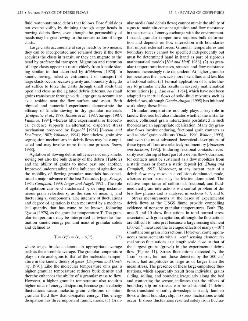
Virtually all debris flows move downslope as one ormore unsteady and nonuniform surges. Commonly, anabrupt bore forms the head of the flow, followed by agradually tapering body and thin, more watery tail [e.g.,Pierson, 1986; Takahashi, 1991] (Figure 8). When mul-tiple surges occur in individual debris flows, each exhib-its a conspicuous head and tail [Jahns, 1949; Sharp andNobles, 1953; Pierson, 1980; Davies, 1988, 1990]. Graphsof flow depth or discharge versus time illustrate thegenerally irregular character of these surges (Figure 9)[Takahashi, 1991; Khegai et al., 1992; Ohsumi WorksOffice, 1995]. Observations during experiments at theUSGS debris flow flume show that surges can arise

spontaneously, without extraneous perturbations of theflow. The resulting low-amplitude surface waves resem-ble roll waves that form in open channel flows of wateron steep slopes [e.g., Henderson, 1966]. In experimentaldebris flows, larger waves tend to overtake and canni-balize smaller waves, as may be anticipated from kine-matic wave theory [Lighthill and Whitham, 1955]. Con-sequent coalescence of wave fronts can produce asequence of large-amplitude surges, which may them-selves become unstable. Although other processes, suchas transient damming or episodic slope failures, mightalso generate surges [Jahns, 1949], intrinsic flow insta-bility and wave coalescence suffice.

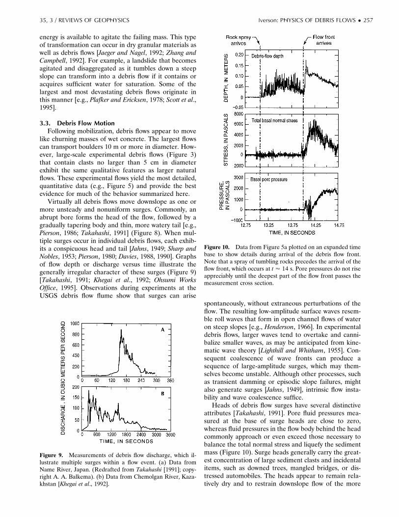
Heads of debris flow surges have several distinctiveattributes [Takahashi, 1991]. Pore fluid pressures mea-sured at the base of surge heads are close to zero,whereas fluid pressures in the flow body behind the headcommonly approach or even exceed those necessary tobalance the total normal stress and liquefy the sedimentmass (Figure 10). Surge heads generally carry the great-est concentration of large sediment clasts and incidentalitems, such as downed trees, mangled bridges, or dis-tressed automobiles. The heads appear to remain rela-tively dry and to restrain downslope flow of the more

Figure 9. Measurements of debris flow discharge, which il-lustrate multiple surges within a flow event. (a) Data fromName River, Japan. (Redrafted from Takahashi [1991]; copy-right A. A. Balkema). (b) Data from Chemolgan River, Kaza-khstan [Khegai et al., 1992].

Figure 10. Data from Figure 5a plotted on an expanded timebase to show details during arrival of the debris flow front.Note that a spray of tumbling rocks precedes the arrival of theflow front, which occurs at t ' 14 s. Pore pressures do not riseappreciably until the deepest part of the flow front passes themeasurement cross section.


fluid, water-saturated debris that follows. Pore fluid doesnot escape visibly by draining through surge heads inmoving debris flows, even though the permeability ofheads may be great owing to the concentration of largeclasts.

Large clasts accumulate at surge heads by two means:they can be incorporated and retained there if the flowacquires the clasts in transit, or they can migrate to thehead by preferential transport. Migration and retentionof large clasts appear to result chiefly from kinetic siev-ing similar to that described by Middleton [1970]. Inkinetic sieving, selective entrainment or transport oflarge clasts occurs because gravity and boundary drag donot suffice to force the clasts through small voids thatopen and close as the agitated debris deforms. As smallgrains translocate through voids, large grains accumulateas a residue near the flow surface and snout. Bothphysical and numerical experiments demonstrate theefficacy of kinetic sieving in dry granular materials[Bridgwater et al., 1978; Rosato et al., 1987; Savage, 1987;Vallance, 1994], whereas little experimental or theoreti-cal evidence supports an alternative, dispersive stressmechanism proposed by Bagnold [1954] [Iverson andDenlinger, 1987; Vallance, 1994]. Nonetheless, grain sizesegregation mechanisms in debris flows may be compli-cated and may involve more than one process [Suwa,1988].

Agitation of flowing debris influences not only kineticsieving but also the bulk density of the debris (Table 2)and the ability of grains to move past one another.Improved understanding of the influence of agitation onthe mobility of flowing granular materials has consti-tuted a major advance of the last 2 decades [e.g., Savage,1984; Campbell, 1990; Jaeger and Nagel, 1992]. The roleof agitation can be characterized by defining instanta-neous grain velocities vs as the sum of mean vs andfluctuating v9s components. The intensity of fluctuationsand degree of agitation is then measured by a mechan-ical quantity that has come to be known, followingOgawa [1978], as the granular temperature T. The gran-ular temperature may be interpreted as twice the fluc-tuation kinetic energy per unit mass of granular solidsand defined as

T 5 ^v9s2& 5 ^vs 2 vs!

2& (7)

where angle brackets denote an appropriate averagesuch as the ensemble average. The granular temperatureplays a role analogous to that of the molecular temper-ature in the kinetic theory of gases [Chapman and Cowl-ing, 1970]. Like the molecular temperature of a gas, ahigher granular temperature reduces bulk density andthereby enhances the ability of a granular mass to flow.However, a higher granular temperature also requireshigher rates of energy dissipation, because grain velocityfluctuations cause inelastic grain collisions or inter-granular fluid flow that dissipates energy. This energydissipation has three important ramifications: (1) Gran-

ular media (and debris flows) cannot mimic the ability ofa gas to maintain constant agitation and flow resistancein the absence of energy exchange with the environment.Instead, granular temperature requires bulk deforma-tion and depends on flow interaction with boundariesthat impart external forces. Granular temperatures andboundary forces cannot be specified independently butmust be determined hand in hand as part of rigorousmathematical models [Hui and Haff, 1986]. (2) As gran-ular temperature increases, stresses and flow resistancebecome increasingly rate dependent. At higher granulartemperatures the mass acts more like a fluid and less likea frictional solid. (3) Formal application of kinetic the-ory to granular media results in severely mathematicalformulations [e.g., Lun et al., 1984], which have not beenadapted to inertial flows of solid-fluid mixtures such asdebris flows, although Garcia-Aragon [1995] has initiatedwork along these lines.

Granular temperature not only plays a key role inkinetic theories but also indicates whether the instanta-neous, collisional grain interactions postulated in suchtheories are an appropriate idealization. Many dry gran-ular flows involve enduring, frictional grain contacts aswell as brief grain collisions [Drake, 1990; Walton, 1993],and even the most advanced theoretical descriptions ofthese types of flows are relatively rudimentary [Andersonand Jackson, 1992]. Enduring frictional contacts neces-sarily exist during at least part of a debris flow’s duration,for contacts must be sustained as a flow mobilizes froma static mass or forms a static deposit [cf. Zhang andCampbell, 1992]. Moreover, at any instant, part of adebris flow may move in a collision-dominated mode,whereas other parts may be friction dominated. Therelative importance of collisional, frictional, and fluid-mediated grain interactions is a central problem of de-bris flow physics and is analyzed in sections 4, 7, and 8.

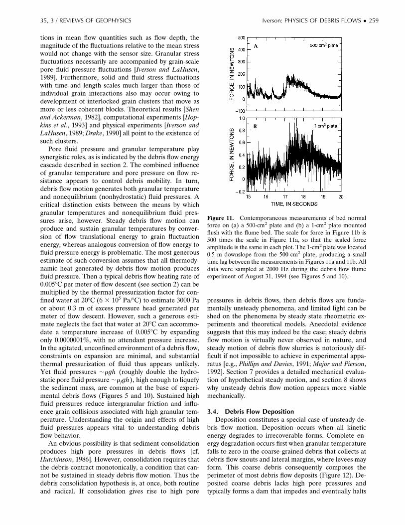
Stress measurements at the bases of experimentaldebris flows at the USGS flume provide compellingevidence of nonzero granular temperatures. Both Fig-ures 5 and 10 show fluctuations in total normal stressassociated with grain agitation, although the fluctuationsare difficult to interpret because a large sensing element(500 cm2) measured the averaged effects of many (;105)simultaneous grain interactions. However, contempora-neous measurements with a 1-cm2 sensing element re-veal stress fluctuations at a length scale close to that ofthe largest grains (gravel) in the experimental debrisflow (Figure 11). Stress fluctuations detected by the1-cm2 sensor, but not those detected by the 500-cm2

sensor, had amplitudes as large as or larger than themean stress. The presence of these large-amplitude fluc-tuations, which apparently result from individual grainssliding, rolling, and bouncing irregularly along the bedand contacting the sensor, indicates that the effects ofboundary slip on stresses can be substantial. If debrisflows translated smoothly downslope as steady, laminarflows without boundary slip, no stress fluctuations wouldoccur. If stress fluctuations resulted solely from fluctua-


tions in mean flow quantities such as flow depth, themagnitude of the fluctuations relative to the mean stresswould not change with the sensor size. Granular stressfluctuations necessarily are accompanied by grain-scalepore fluid pressure fluctuations [Iverson and LaHusen,1989]. Furthermore, solid and fluid stress fluctuationswith time and length scales much larger than those ofindividual grain interactions also may occur owing todevelopment of interlocked grain clusters that move asmore or less coherent blocks. Theoretical results [Shenand Ackerman, 1982], computational experiments [Hop-kins et al., 1993] and physical experiments [Iverson andLaHusen, 1989; Drake, 1990] all point to the existence ofsuch clusters.

Pore fluid pressure and granular temperature playsynergistic roles, as is indicated by the debris flow energycascade described in section 2. The combined influenceof granular temperature and pore pressure on flow re-sistance appears to control debris mobility. In turn,debris flow motion generates both granular temperatureand nonequilibrium (nonhydrostatic) fluid pressures. Acritical distinction exists between the means by whichgranular temperatures and nonequilibrium fluid pres-sures arise, however. Steady debris flow motion canproduce and sustain granular temperatures by conver-sion of flow translational energy to grain fluctuationenergy, whereas analogous conversion of flow energy tofluid pressure energy is problematic. The most generousestimate of such conversion assumes that all thermody-namic heat generated by debris flow motion producesfluid pressure. Then a typical debris flow heating rate of0.0058C per meter of flow descent (see section 2) can bemultiplied by the thermal pressurization factor for con-fined water at 208C (6 3 105 Pa/8C) to estimate 3000 Paor about 0.3 m of excess pressure head generated permeter of flow descent. However, such a generous esti-mate neglects the fact that water at 208C can accommo-date a temperature increase of 0.0058C by expandingonly 0.0000001%, with no attendant pressure increase.In the agitated, unconfined environment of a debris flow,constraints on expansion are minimal, and substantialthermal pressurization of fluid thus appears unlikely.Yet fluid pressures ;rgh (roughly double the hydro-static pore fluid pressure ;rfgh), high enough to liquefythe sediment mass, are common at the base of experi-mental debris flows (Figures 5 and 10). Sustained highfluid pressures reduce intergranular friction and influ-ence grain collisions associated with high granular tem-perature. Understanding the origin and effects of highfluid pressures appears vital to understanding debrisflow behavior.

An obvious possibility is that sediment consolidationproduces high pore pressures in debris flows [cf.Hutchinson, 1986]. However, consolidation requires thatthe debris contract monotonically, a condition that can-not be sustained in steady debris flow motion. Thus thedebris consolidation hypothesis is, at once, both routineand radical. If consolidation gives rise to high pore

pressures in debris flows, then debris flows are funda-mentally unsteady phenomena, and limited light can beshed on the phenomena by steady state rheometric ex-periments and theoretical models. Anecdotal evidencesuggests that this may indeed be the case; steady debrisflow motion is virtually never observed in nature, andsteady motion of debris flow slurries is notoriously dif-ficult if not impossible to achieve in experimental appa-ratus [e.g., Phillips and Davies, 1991; Major and Pierson,1992]. Section 7 provides a detailed mechanical evalua-tion of hypothetical steady motion, and section 8 showswhy unsteady debris flow motion appears more viablemechanically.

3.4. Debris Flow DepositionDeposition constitutes a special case of unsteady de-

bris flow motion. Deposition occurs when all kineticenergy degrades to irrecoverable forms. Complete en-ergy degradation occurs first when granular temperaturefalls to zero in the coarse-grained debris that collects atdebris flow snouts and lateral margins, where levees mayform. This coarse debris consequently composes theperimeter of most debris flow deposits (Figure 12). De-posited coarse debris lacks high pore pressures andtypically forms a dam that impedes and eventually halts

Figure 11. Contemporaneous measurements of bed normalforce on (a) a 500-cm2 plate and (b) a 1-cm2 plate mountedflush with the flume bed. The scale for force in Figure 11b is500 times the scale in Figure 11a, so that the scaled forceamplitude is the same in each plot. The 1-cm2 plate was located0.5 m downslope from the 500-cm2 plate, producing a smalltime lag between the measurements in Figures 11a and 11b. Alldata were sampled at 2000 Hz during the debris flow flumeexperiment of August 31, 1994 (see Figures 5 and 10).


the motion of ensuing finer-grained debris that retainshigher pore pressures. Alternatively, wetter, more mo-bile debris may have enough momentum to override orbreach the dam of previously deposited debris, so thatdeposits can develop by a combination of forward push-ing, mass “freezing,” vertical accretion, and lateralshunting of previously deposited sediment [Major, 1997].Experimental observations of idealized debris mixturesindicate that freezing generally occurs from the bottomup, rather than the top down, as debris comes to rest[Vallance, 1994]. Thus neither the thickness of depositedlobes nor that of levees provides a good indicator of thedynamic behavior of the moving debris as a whole [cf.Johnson, 1970]. Instead, the complex interplay betweenthe resistance of the first-deposited debris and the mo-mentum of subsequently arriving debris produces depos-its that are initially dry and strong at their perimeter, wetand weak in their interior, and conspicuously heteroge-neous in their resistance to motion. Indeed, pore fluidpressures in the center of a deposit can remain elevatedwell above hydrostatic levels and maintain the sedimentin a nearly liquefied state long after deposition occurs

(Figure 13) [Major, 1996] [cf. Hampton, 1979; Pierson,1981]. Subsequent decay of interior pore pressures, withattendant consolidation (i.e., gravitational settling) ofthe solids and drainage of fluid, marks the final stages ina debris flow’s transition from fluid-like to solid-likebehavior.

The timescale for pore pressure decay is defined bythe quotient of a pore pressure diffusion coefficient,D 5 kE/m, and the square of the characteristic drainagepath length. Here E is the composite stiffness (reciprocalof the compressibility) of the debris mixture. Measure-ments and modeling by Major [1996] show that drainageis dominantly vertical in typical debris flow deposits,which have lengths and widths that greatly exceed theirthickness h. Thus the characteristic drainage path lengthis h, which yields the pore pressure diffusion timescale

tdif 5 h2m/kE (8)

Because high pore pressures help sustain debris mobil-ity, it is tempting to equate the diffusion timescale tdiffwith the debris flow duration or timescale for whichmobility is sustained, tD [Hutchinson, 1986]. Three prob-lems complicate this interpretation, however. First, porefluid pressures are but one phenomenon that influencesmobility; debris flow mixtures can flow in the absence ofhigh pore pressure if they have sufficient granular tem-perature. Second, nonequilibrium pore pressures may besmall or absent at the front of debris flow surges (Figures5 and 10), so that pore pressure diffusion is locallyirrelevant. Finally, the definition of tdiff includes a com-posite stiffness coefficient E, which has the properties ofan elastic modulus in small-strain problems [Biot, 1941]but which has more complicated properties when defor-mations are large and irreversible [e.g., Helm, 1982].Section 8 addresses this issue quantitatively and showshow the evolving compressibility of debris flow materialscan influence pore pressure diffusion and play a key rolein debris flow physics.

4. MOMENTUM TRANSPORT:SCALING AND DIMENSIONAL ANALYSIS

To build a quantitative background for analyzing de-bris flow physics, it is useful to ignore temporarily someof the complexities described in the preceding sectionand consider momentum transport during steady, simpleshearing of an unbounded, uniform mixture of identical,dense spherical grains and water. Initially restrictingattention to an unbounded domain and a single graindiameter d vastly simplifies the analysis, because it un-ambiguously establishes the dominant length scale as d.Scaling considerations then suffice to draw rudimentaryconclusions about momentum transport and the atten-dant state of stress in the mixture. Associated dimen-sional analysis defines dimensionless parameters thatcan be used to classify debris flows and identify limiting

Figure 12. Photographs of snouts of debris flow deposits,which show concentrations of coarse clasts and bluntly taperedmargin morphology. (a) Lobe of a small (;1000 m3) debrisflow that partly crossed the scenic highway near Benson StatePark, Oregon, February 7, 1996. (b) Vertical cross sectionthrough a marginal lobe of an experimental debris flow at theUSGS debris flow flume, October 8, 1992.


styles of behavior. The multiplicity of relevant dimen-sionless parameters also reveals why nearly intractableproblems arise in attempts to “scale down” debris flowmixtures to the size of laboratory apparatus. Such scalingproblems may partly explain why very divergent viewsabout debris flow physics have arisen from differentapproaches to experimentation and modeling (see sec-tion 5).

Figure 14 depicts schematically a representative re-gion within a uniform grain-water mixture undergoingsteady, uniform shearing motion in a gravity field; the

various stresses (solid grain shear and normal stress,fluid shear and normal stress, and solid-fluid interactionstress) that accompany momentum transport in the mix-ture are represented collectively by S. Adapting theapproach used by Savage [1984] for dry grain flows, thesestresses are postulated to depend functionally on themixture shear rate g and on 12 additional variablesdiscussed in section 3 and listed in the notation section:

S 5 ^~g, d, rs, rf, g, m, k, T, E, ys, yf, f, e! (9)

Variables not included in (9) might influence stressesalso but are assumed to have less importance than thoseincluded.

As a preliminary step, dimensional analysis reorga-nizes (9) into a more fundamental and compact relation-ship that involves only dimensionless parameters. Thefirst 10 variables in (9) have units comprising threephysical dimensions: mass, length, and time. The lastfour variables in (9) are intrinsically dimensionless andare superfluous in dimensional analysis. According tothe Buckingham II theorem [Buckingham, 1915], anyphysically meaningful relation between 10 variablescomprising three dimensions must reduce to a relationbetween 7 (5 10 2 3) independent dimensionless pa-rameters. Definition of these parameters depends onchoices for the characteristic length, mass, and time. Forthe simple system depicted in Figure 14, the choices areobvious: the characteristic length is d, the characteristicmass is rsd

3, and the characteristic time is 1/g. These, inturn, determine a characteristic velocity v ; gd, whichdescribes the speed at which grains move past one an-

Figure 13. Measurements of total basal normal stress (on a 500-cm2 plate) and basal pore pressure duringdeposition of debris flow sediments with different grain size distributions at the USGS debris flow flume.Measurements were made through ports in the runout pad at the flume base (Figure 4), and deposits werecentered over the measurement ports. Deposit interiors were liquefied by high pore pressure at the time ofemplacement, and pore pressures subsequently decayed. High pore pressures persisted much longer in thedeposit that contained loam with about 6% (by weight) silt and clay-sized particles than in the deposit thatlacked loam and contained about 2% (by weight) silt and clay-sized particles [after Major, 1996].

Figure 14. Schematic diagram of a steady, uniform, un-bounded shear flow of identical solid spheres immersed in aNewtonian fluid. This flow is too simple to represent debrisflows, but it provides a basis for assessing scaling parametersthat influence stresses.


other and at which fluid moves to accommodate grainmotion. With these choices, standard methods of dimen-sional analysis [e.g., Bridgman, 1922] applied to (9) yield

S

g2d2rs5 ^Sg2d

g,

gd2rs

m,

rs

rf,

T

g2d2 ,kd2 ,

Eg2d2rs

D (10)

The right-hand side of this relation lists six dimension-less parameters that determine the dimensionlessstresses, S/g2d2rs. The significance of the first right-hand-side parameter was first enunciated by Savage[1984], and accordingly it has been dubbed the Savagenumber [Iverson and LaHusen, 1993]. The second pa-rameter is a variation of a parameter first investigated byBagnold [1954], commonly called the Bagnold number[Hill, 1966]. The third parameter is the ratio of soliddensity to fluid density, which ranges only from about 2to 3 in debris flows. The fourth parameter is the granulartemperature scaled by the square of the characteristicshear velocity gd [cf. Savage, 1984]. The fifth parameteris the permeability divided by the grain diametersquared; it reflects the role that grain size and packingplay in solid-fluid interactions. The sixth parameter isthe composite mixture stiffness (resistance to dilationand contraction) divided by the characteristic stressg2d2rs.

The significance of the parameters in (10) can beclarified by analyzing their relationship to estimates ofsolid, fluid, and solid-fluid interaction stresses in themixture. These stresses have both shear and normalcomponents; in turn, each of these components mayhave both quasi-static and inertial components. Forbrevity, this analysis will focus exclusively on shear com-ponents of stress, which are generally of greatest inter-est. A similar analysis is easily conducted for the normalstress components.

The solid inertial stress Ts(i) and fluid inertial stressTf(i) both scale like the product of the mass (solid orfluid) per unit volume and the square of the character-istic velocity, v2 ; g2d2. Thus they may be estimated by

Ts~i! , ysrsg2d2 (11)

Tf~i! , yfrfg2d2 (12)

The first of these relationships shows that the character-istic stress used to scale S in (10) is essentially the solidgrain inertia stress. This is the stress transmitted by graincollisions [cf. Iverson and Denlinger, 1987] and explicatedby Bagnold [1954]. The second relationship shows thatfluid can also sustain inertial stresses, in a mannerroughly analogous to that of Reynolds stresses in turbu-lent flow of pure fluid. The fluid-inertia stress was ig-nored by Bagnold [1954].

The quasi-static solid stress Ts(q) is associated withCoulomb sliding and enduring grain contacts (see equa-tion (6)). This stress increases as depth below a horizon-tal datum increases but decreases if static pressure in the

adjacent fluid increases independently. At depth Nd thequasi-static solid stress is estimated by

Ts~q! , Nys~rs 2 rf! gd tan f (13)

where N, the number of grains above and including thelayer of interest, accounts for the effects of the overbur-den load, and ys(rs 2 rf) g is the buoyant unit weight ofthis overburden. Additional (nonhydrostatic) fluid pres-sure may also mediate Ts(q) but is characterized sepa-rately (below) by the solid-fluid interaction stress, Ts2f.

The quasi-static fluid stress derives from Newton’slaw of viscosity:

Tf~q! 5 yfgm (14)

In this equation, yf appears because only this fraction ofthe mixture undergoes viscous shear.

The solid-fluid interaction stress Ts2f results fromrelative motion of the solid and fluid constituents. Al-though Ts2f may involve both inertial and quasi-static(viscous drag) components, a detailed analysis by Iverson[1993] shows that viscous coupling surpasses inertialcoupling in materials similar to those in debris flows, andthat neglect of inertial coupling is generally justified.Viscous coupling results in drag that generates a forceper unit volume of mixture ;v(m/k), which produces astress ;vd(m/k). Thus, expressed in terms of the shearrate g 5 v/d, the interaction stress can be estimated as

Ts2f ,gmd2

k (15)

This interaction stress results from grain-scale fluid flowdriven by grain rearrangements during steady shearingmotion at the rate g [cf. Iverson and LaHusen, 1989]. Ifmotion were unsteady and net volume change were tooccur, an additional viscous interaction stress wouldarise in concert with net pore pressure diffusion (seediscussion following equation (8)).

The chief significance of (11)–(15) lies in the ratiosthat they form. For example, division of the character-istic stress Ts(i) by Ts(q) shows that a Savage numberNSav (here modified to account for the solid frictionangle, overburden load, and hydrostatic buoyancy) maybe defined by the ratio of inertial shear stress associatedwith grain collisions to quasi-static shear stress associ-ated with the weight and friction of the granular mass

NSav 5g2rsd

N~rs 2 rf! g tan f(16)

Similarly, division of Ts(i) by Tf(q) shows that a Bagnoldnumber NBag may be defined by the ratio of inertialgrain stress to viscous shear stress:

NBag 5ys

1 2 ys

rsd2g

m(17)

wherein the factor ys/(1 2 ys) results from the substi-tution yf 5 1 2 ys and differs from the factor l1/ 2 5


[ys1/3/(y*

1/3 2 ys1/3)]1/ 2 originally used by Bagnold [1954]

(y* is the maximum value of ys achievable in a dense-packed configuration). Division of Ts(i) by Tf(i) producesa “mass number” Nmass that describes the ratio of solidinertia to fluid inertia in the mixture:

Nmass 5ys

1 2 ys

rs

rf(18)

Division of Ts2f by Ts(i) produces a quantity heretermed the “Darcy number,”

NDar 5m

ysrsgk (19)

which describes the tendency for pore fluid pressuredeveloped between moving grains to buffer grain inter-actions. Furthermore, division of NDar by E/(g2d2rs)(which appears in (10)), yields (gmd2)/(yskE), a dimen-sionless parameter that describes the ratio of the time-scale for diffusive pore pressure dissipation across thedistance d to the timescale for pore pressure generationby grain interactions, 1/g [cf. Iverson and LaHusen,1989]. The diffusion timescale md2/kE resembles theconsolidation timescale defined in (8). The chief differ-ence is that md2/kE characterizes grain-scale diffusion ina flow that is macroscopically steady, whereas (8) char-acterizes diffusion during unsteady consolidation through-out the entire debris flow thickness.

Additional dimensionless parameters of interest canbe obtained by forming ratios of the parameters definedin (16)–(19). For example, a version of the well-knowngrain Reynolds number can be expressed as

NRey 5NBag

Nmass5

rfgd2

m(20)

and the ratio of the Bagnold number to Savage numberforms a version of the friction number identified byIverson and LaHusen [1993]:

Nfric 5NBag

NSav5

ys

1 2 ys

N~rs 2 rf! gd tan f

gm(21)

This number expresses the ratio of shear stress borne bysustained grain contacts to viscous shear stress. It resem-bles the well-known Bingham number, which describesthe ratio of stress borne by shear strength to stress borneby viscous flow in viscoplastic materials. The key differ-ence between the friction number and Bingham numberlies in the fact that the friction number characterizesstresses borne by distinct solid and fluid phases, whereasthe Bingham number characterizes stresses in a one-phase material that exhibits both viscosity and strength.

The dimensionless groups defined by (16)–(21) dis-tinguish five processes of momentum transport (i.e.,stress generation) in a steady shear flow of a uniformmixture of identical grains and water: (1) inertial graincollisions, (2) grain contact friction, (3) viscous shear, (4)inertial (turbulent) fluid velocity fluctuations, and (5)

solid-fluid interactions. At least this many processesmust affect stresses in debris flows with more compli-cated constituents and kinematics [Iverson and Den-linger, 1987]. It thus appears unlikely that any simplerheological model can accurately represent all stresses indebris flows. Nonetheless, simple but valid approxima-tions may be attainable if in some circumstances only asubset of these stresses dominate.

Rough but useful assessments of the relative impor-tance of different stress generation mechanisms in de-bris flows can be accomplished by calculating represen-tative values of the dimensionless parameters defined in(16)–(21) and comparing these values with those forsimpler systems in which stress generation is better un-derstood. This process is analogous to assessing openchannel flow of water on the basis of Froude and Reyn-olds numbers. Table 5 lists values of (16)–(21) computedfor a representative spectrum of debris flows, rangingfrom a 10-m3 flow in the USGS flume to the prehistoricOsceola mudflow of ;109 m3 (see Table 1). Values ofsome variables need to be estimated to make thesecomputations. For example, Table 5 lists a fixed d of 1mm for all flows. Although all flows listed in Table 5consisted predominantly of grains of about this size(sand), larger grains might be more significant in someinstances (as in a boulder- or cobble-rich debris flowsnout). Nonetheless, the values of (16)–(21) listed inTable 5 provide some idea of the range of values for avariety of debris flows.

Although interpretation of the values of (16)–(21) inTable 5 is limited by a dearth of relevant data, someguidelines exist. For example, Savage and Hutter [1989]reviewed a variety of experimental evidence and con-cluded that grain collision stresses dominate grain fric-tion stresses in dry granular flows if NSav is greater thanabout 0.1. Similarly, Bagnold’s [1954] experiments dem-onstrated that in neutrally buoyant mixtures of sphericalgrains and liquid (where NSav 3 `), collisional stressesdominate viscous stresses if NBag exceeds roughly 200.(This differs from Bagnold’s [1954] value of 450, becauseBagnold included the factor l1/2 rather than ys/(1 2 ys)in his evaluation.) Apparently no experimental databearing on transition values of Nmass are available, al-though the qualitative influence of Nmass is obvious fromits definition: grain inertia becomes unimportant as thedensity or concentration of grains approaches zero. Incontrast, many data pertain to grain Reynolds numbers,NRey. Typically, fluid flow with respect to grains beginsto show inertial effects and deviate significantly fromideal viscous (Stokesian) behavior for NRey . 1 [Vanoni,1975]. Fewer data are available for Nfric and NDar, al-though Iverson and LaHusen [1989] reported experi-ments with 1000 , NDar , 6000, in which large fluidpressure fluctuations evidenced strong solid-fluid inter-actions. Values of NDar at least this large probably applyfor most debris flows (Table 5).

With these guidelines for interpretation, the tabu-lated values of dimensionless parameters in Table 5


paint a reasonably consistent picture of the factors apt toinfluence stresses in debris flows. For thin, fast flows onsteep slopes (e.g., flows at the USGS debris flow flume),high shear rates cause both the Savage number andBagnold number to be moderately large; however, thetabulated values NSav 5 0.2 and NBag 5 400 approximatethe respective transition values 0.1 and 200. Thus graincollisions might be expected to transmit most stress insuch flows, but friction and viscosity also may contributesignificantly. For larger flows with greater depths andsmaller shear rates, the situation is more clear-cut. Smallvalues of NSav and NBag indicate that collisions likelytransmit negligible stress in such flows and that frictionand viscosity dominate. Large values of the friction num-ber suggest that frictional shear stresses probably exceedviscous shear stresses, but small grain Reynolds numbersand large values of NDar indicate that viscous drag asso-ciated with solid-fluid interactions is likely to be impor-tant. The picture changes in parts of debris flows (suchas heads of surges) where grains coarser than sandpredominate. If shear rates are constant and d increases,friction increasingly dominates viscosity, but collisionsincreasingly dominate friction. Thus individual debrisflows may include regions where different momentumtransport processes dominate or where several processescontribute almost equally. With this knowledge, modelsthat include only one or two processes of momentum

transport (such as those described in sections 5 and 9)can be placed in an appropriate context.

In principle, the values of key dimensionless param-eters also facilitate discrimination of debris flows fromrelated phenomena. For example, by selecting the pa-

Figure 15. Classification scheme that distinguishes debrisflows on the basis of values of the dimensionless parametersNSav, NBag, and NDar. Debris flows occupy a broad and impre-cisely defined domain (shaded) in the center of this parameterspace. If one or more of the parameters NSav, NBag, and NDar

has a value either very large or small, debris flow may gradeinto other types of sediment transport processes, as indicatedby labeled regions in the diagram.

TABLE 5. Estimation of Dimensionless Parameters That Characterize Stresses in a Range of PrototypicalDebris Flow Mixtures

Parameter

Debris Flow Prototype

USGS Flume Experiment(Sand-Gravel)

Oddstad Debris Flow(Figure 1), Jan. 4, 1982

South Toutle River,May 18, 1980

Osceola Mudflow,circa 5700 B.P.

Dimensional Parametersd, m 0.001* 0.001* 0.001* 0.001*h 5 Nd, m 0.1 1 5 20v, m/s 10 10 20 20g, 1/s 100 10 4 1rs, kg/m3 2700 2700 2700 2700rf, kg/m3 1100 1100 1100 1200m, Pa s 0.001 0.01* 0.01* 0.1*g, m/s2 9.8 9.8 9.8 9.8k, m2 10211 10211* 10212 10212

E, Pa 104* 104* 104* 104*ys 0.6 0.6 0.6 0.6yf 0.4 0.4 0.4 0.4f, deg 40 30 30 30

Dimensionless ParametersNSav 0.2 2 3 1024 6 3 1026 1 3 1027

NBag 400 4 0.2 0.4Nmass 4 4 4 4NDar 600 60,000 2 3 106 6 3 107

NRey 100 1 0.04 0.01Nfric 2 3 103 2 3 104 3 3 104 4 3 105

Data sources for approximate range of values of dimensional parameters are as follows: h, v, and g, kinematic reconstructions and directobservations (see references cited in Table 1); rf, rs, m, k, ys, and yf, Table 2, Table 4, and Figure 6 of this paper; d, E, and f, Figure 20 ofthis paper and data from Major [1996]. In all cases the typical shear rate g is estimated from the quotient of the typical flow speed v and depth,h.

*Values of dimensional parameters for which the tabulated value may vary or err by more than an order of magnitude.


rameters NSav, NBag, and NDar as those most likely tovary significantly from flow to flow, a classificationscheme such as that shown in Figure 15 can be devised.In this scheme various phenomena that can resembleand transform to or from debris flows, such as rockavalanches or turbidity currents, represent limiting casesin which one or more of the parameters NSav, NBag, andNDar has a value that is either very large or very small.The parameter space intermediate between these limit-ing cases includes the variety of behaviors that constitutethe process of debris flow. At present, such a classifica-tion has utility chiefly as a conceptual tool; it illustratesthe hybrid character of debris flows and indicates thatdebris flow behavior likely cannot be discriminated onthe basis of a few simple measures, such as shear rateand solids concentration. A more rigorous interpretationremains elusive because the parameter space boundariesbetween various processes identified in Figure 15 remainvaguely defined.

Although the appeal of simple dimensional methodsand classifications is clear, it is important to recognizetheir limitations. Because the foregoing dimensionalanalysis assumes very idealized kinematics (uniform sim-ple shear flow), it neglects variations in granular tem-perature and volume fraction, and it neglects energyconversion and dissipation that necessarily occur at flowboundaries. Perhaps most importantly, it neglects thatdebris flows virtually always include grains of widelyranging sizes, develop pore pressures that exceed hydro-static values, and occur as unsteady, nonuniform surges.Analyses more sophisticated than simple scaling anddimensional methods are therefore needed to developbetter insight and appropriate models. The followingsections describe traditional and more recent ap-proaches to this problem.

5. TRADITIONAL (RHEOLOGICAL) MODELSOF MOMENTUM TRANSPORT

Models of two distinct types, viscoplastic and inertialgrain flow, traditionally have provided the theoreticalframework for most debris flow research. Each type ofmodel postulates a unique rheological relation betweenthe shear stress and shear strain rate in flowing debrismixtures. Such postulates conflict with data showing thatsolid and fluid stresses in debris flows vary asynchro-nously (Figures 5, 10, and 13) and with inferences thatvarying pore pressures and granular temperatures influ-ence debris behavior. Consequently, this section avoidsdetailed review of traditional rheological models (pro-vided previously by Johnson [1984] and Takahashi[1991]), and instead summarizes their strengths andshortcomings. Table 6 compares qualitative attributes ofdebris flows that can be explained with traditional mod-els and a model that emphasizes solid-fluid interactions.Later sections of this paper provide a more quantitativeperspective.

The first systematic efforts to develop a physical un-derstanding of debris flows were those of Johnson [1965]and Yano and Daido [1965], who recognized indepen-dently that debris flows exhibit properties of both viscousfluids and plastic solids. This marked a significant stepforward, because earlier, descriptive work did not clearlydistinguish the mechanics of debris flows from those ofmuddy water floods. Johnson [1965, 1970, 1984] adoptedthe simplest mechanical model that combines plastic andviscous attributes: that of a Bingham, or viscoplastic,continuum [cf. Bird et al., 1982]. This model describes asingle-phase material that remains rigid or elastic unlessdeviatoric stresses exceed a threshold value, the plasticyield strength. Where stresses exceed the yield strength,

TABLE 6. Comparison of Models’ Ability to Explain Physical Phenomena That Typify Debris Flows

Phenomenon

Type of Model

BinghamViscoplastic

BagnoldGrainFlow

Coulomb GrainFlow With

Variable PorePressure

Flow mobilizes from rigid slope failure without changes in constitutive properties XFluid pressures in flow can differ from the mean pressure and affect apparent

strength or flow resistanceX

Flow can exhibit a “rigid” plug of undeforming material X XFlow can lack a “rigid” plug of undeforming material X XFlow is unsteady and nonuniform, with a blunt snout and tapered tail X X XFlow can transport large clasts that do not settle out X X XFlow produces grain size segregationFlow agitation can affect apparent strength or flow resistance XBoundary slip occurs at the bed XFlow strengthens and halts rapidly when pore fluid is drained from beneath it XDeposit interior can remain weak and unable to support loads while deposit

perimeter becomes rigidX

‘‘X’’ denote phenomena that can be explained at least qualitatively. Assessment of the Bingham and Bagnold models assumes that thestandard forms as described by Johnson [1984] and Takahashi [1981] apply. The model of Coulomb grain flow with variable pore pressure isdescribed in section 9 of this paper.


the material flows like a viscous fluid. At a stress-freesurface of an open channel flow such as a debris flow, aBingham material translates like a rigid solid.

As was recognized by Johnson [1965, 1970, 1984],Bingham models for debris flows can be generalized toallow yield strength to depend on Coulomb friction (andhence on the mean stress) and viscosity to depend ondeformation rate [Iverson, 1985; Coussot and Piau, 1994,1995], but applications of Bingham models to debrisflows have almost invariably assumed fixed viscositiesand yield strengths [e.g., Fink et al., 1981]. Most appli-cations have also assumed steady, uniform flow. Forexample, steady state balances of driving and resistingforce have been used to infer fixed yield strengths fromthe thickness of deposited debris flow lobes [Johnson,1984; Whipple and Dunne, 1992]. Bingham strengthstreated in this manner are equivalent both conceptuallyand mathematically to Coulomb strengths (equation (6))in which f 5 0 and cohesion alone controls yielding. Ifthis equivalency has a sound physical basis, Binghamstrengths should increase as the fines content of thedebris increases, and small-scale experiments with debrismixtures composed of only fine sediment and waterindeed produce this behavior [Johnson, 1970; O’Brienand Julien, 1988; Major and Pierson, 1992]. However,large-scale flume experiments with mixtures of predom-inantly sand, gravel, and water, with a fines content ofonly a few percent (comparable to most natural debrisflow mixtures) show that increased fines content de-creases lobe thickness and apparent strength, becausethe fines help sustain high pore pressures that reducefrictional resistance and enhance lobe spreading [Major,1996]. This reveals a fundamental shortcoming of fixed-yield-strength Bingham models: such models simulatethe rheology of the water-plus-fines fraction of debris-flow mixtures, whereas observations and data show thatinteractions of coarse sediment grains with one anotherand with adjacent fluid strongly affect debris flow behav-ior [cf. Costa and Williams, 1984; Major and Pierson,1992].

Even if posed and used in a very general form [Iver-son, 1985, 1986a, b], Bingham models have significantlimitations [cf. Johnson, 1984]. They assume that mo-mentum transport and energy dissipation in debris flowsoccurs exclusively by viscous shearing. They neglect thefact that rate-independent energy dissipation can occurwhen sediment grains contact one another or flowboundaries [e.g., Adams and Briscoe, 1994], and theyneglect fluid flow relative to the granular assemblage. Inthis respect, Bingham models represent a limiting typeof behavior in which NBag3 0 and NDar3 ` (see Figure15), which may provide an adequate description of phe-nomena such as slow, creeping earthflows but not ofdebris flows. Bingham models also generally employfluid-mechanical no-slip boundary conditions. No-slipboundaries require a Bingham material to leave a con-tinuous layer of deposited sediment along its path, butdebris flow paths commonly lack such deposits. Instead,

grains may slide, collide and roll along flow boundaries.Grains visible on the surface of debris flows may eitherjostle energetically or lock together to form an appar-ently rigid plug, depending on the granular temperature,which in turn depends on flow speed, composition, andboundary conditions. Realistic models of debris flowphysics need to account for these phenomena.

To account for grain interactions, Takahashi [1978,1980, 1981] exploited the seminal findings of Bagnold[1954] to develop an inertial grain flow model of debrisflows. Bagnold’s [1954] experiments employed an en-closed annular shear cell to evaluate the effects of graininteractions in rapidly shearing, concentrated suspen-sions of uniform, solid spheres immersed in a Newtonianfluid of identical density. From his experiments and asimple analysis of binary grain collisions, Bagnold in-ferred that shear and normal stresses in the suspensionsvaried either quadratically or linearly with the shear rate,depending on the value of NBag. Bagnold [1954] used theterms “grain inertia” and “macroviscous,” respectively,to describe the regimes where quadratic and linearstress–strain rate behavior obtained. Subsequent shearcell experiments by others largely confirmed Bagnold’sresults [e.g., Savage and McKeown, 1983] and alsoshowed that the dynamic friction angle relating shearand normal stresses in rapidly shearing granular materi-als differed little from the static Coulomb friction angledescribed by (6) with c 5 0 [e.g., Hungr and Morgenstern,1984; Savage and Sayed, 1984; Sassa, 1985]. Takahashi’s[1978, 1980, 1981] influential contribution to debris flowphysics involved application of Bagnold’s stress–strainrate relations for the grain inertia regime. Other inves-tigators [e.g., Davies, 1986] advocated Bagnold’s [1954]formulas for the macroviscous regime as a model fordebris flows. Unfortunately, use of Bagnold’s [1954] for-mulas for either regime is problematic, for Bagnold’sresults reflect the special conditions of his experiments.Adoption of Bagnold’s [1954] formulas as constitutiveequations for general flow fields leads to contradictoryresults.

Flow of a solid-fluid debris mixture in a channelenclosed by parallel, vertical plates illustrates the type ofcontradictions that can arise in applying Bagnold’s [1954]equations. Flow is driven by a longitudinal body force,such as that due to gravity. Regardless of flow rheology,symmetry dictates that the mixture’s shear rate vanishesat the flow centerline (Figure 16). Bagnold’s equationsfor both the grain inertia and macroviscous regimes thenrequire that the normal and shear stress also vanish atthe centerline. However, a vanishing normal stress con-tradicts the presence of the body force that drives theflow. Bagnold’s experiments lacked this contradictionbecause granular pressure gradients due to gravity orother forces independent of shearing were absent in hisapparatus. In Bagnold’s experiments with neutrallybuoyant spheres, he intentionally camouflaged the effectof gravity on the solid grains, imposed the shear rate,and measured the stress. In debris flows, in contrast,


gravity imparts a stress that increases with depth belowthe surface, and the shear rate responds. Shearing, inturn, can modify the granular pressure gradient by in-fluencing the local granular temperature, grain concen-tration, and possibly the pore-fluid pressure [cf. Hui andHaff, 1986; Johnson et al., 1991]. Thus Bagnold’s results,obtained with fixed concentrations and shear rates, pro-vide valuable insight but not a valid constitutive equationfor debris flows. Section 7 casts this interpretation quan-titatively.

Takahashi’s [1978, 1980, 1981] applications of Bag-nold’s [1954] equations assume that NSav 3 `, that noboundary slip occurs, that grains are uniformly dispersedin the flow, and that interstitial fluid sustains no excesspressure. As a consequence, grain collision stresses mustincrease linearly with depth to balance the gravitationalstress. In turn, this requirement mandates a specificdistribution of shear rate that excludes the possibility of“locked” or unyielding debris that does not shear [cf.,Iverson and Denlinger, 1987]. Not only does this predic-tion contradict observations and the viscoplastic model,it also contradicts the fact that frictionally locked mate-rial must be present during the early and late stages ofdebris flows, when material is mobilized or deposited[Iverson et al., 1997; Major, 1996].

Shortcomings of the viscoplastic and inertial grainflow models have motivated alternative approaches, butnone has produced a widely embraced advance. Oneapproach melds the equations of the viscoplastic andinertial grain flow models [Chen, 1987, 1988a, b]. Thisyields a formulation with numerous adjustable coeffi-cients and with unresolved physical issues, describedabove, that lurk behind the mathematics. A similar ap-proach combines the viscoplastic and grain inertia mod-els in a linear sum without reconciling the models’ phys-ical contradictions [O’Brien et al., 1993]. Otherapproaches abandon the effort to include detailed rheo-logical descriptions, and adopt hydraulic approximationssimilar to that used in water flood routing. Traditionalhydraulic approaches do not consider the dynamics ofdebris mobilization, deformation, and deposition, andinstead use empirical coefficients to parameterize themomentum distribution and energy dissipation inreaches where debris flow is fully developed. Hydraulicformulations that employ depth-averaged “shallow wa-ter” momentum balances [Macedonio and Pareschi,1992; Caruso and Pareschi, 1993; Hunt, 1994] as well askinematic wave approximations [Weir, 1982; Vignaux andWeir, 1990; Arratano and Savage, 1994] have been pre-sented. Calibrated hydraulic models hold promise forpractical forecasts of debris flow speeds and shorelineinundation, but they necessarily neglect key facets ofdebris-flow behavior. Development of improved hydrau-lic models (section 9) requires explicit consideration ofthe physical processes that control mass, momentum,and energy fluxes in debris flows.

6. MASS, MOMENTUM, AND ENERGYCONSERVATION IN DEBRIS FLOW MIXTURES

Mass and linear momentum balances for debris flowscan be borrowed with only minor modification from therelatively mature field of continuum mixture theory [At-kin and Craine, 1976]. Under this rubric, separate butstrongly coupled equations describe mass and momen-tum conservation for the debris flow’s solid and fluidconstituents, and the solid and fluid equations are as-sumed to apply at all locations simultaneously. Angularmomentum equations can also be formulated but arerendered unnecessary by assuming all stress tensors tobe symmetric. Similarly, balances of thermodynamic en-ergy are rendered redundant by assuming the mixture isisothermal. However, an equation for grain fluctuationenergy (granular temperature) may be necessary to de-scribe solid phase motion, and fluid fluctuation energy(turbulence) may be embedded in the fluid momentumequation by including Reynolds stresses.

Figure 16. Schematic diagram depicting steady flow of asolid-fluid mixture between parallel vertical plates. A longitu-dinal body force (e.g., gravity) drives the flow. Depending onthe distribution of granular temperature, a variety of velocityprofiles are possible, including velocity profiles with an appar-ently rigid plug, as shown, but all velocity profiles must have azero velocity gradient at the channel centerline [cf. Hui andHaff, 1986; Johnson et al., 1991]. Consequent zero shear rate atthe centerline invalidates use of Bagnold’s [1954] formulas asconstitutive equations because the equations require zero nor-mal stress in the presence of zero shear rate, which contradictsthe presence of the body force that drives the flow.


The mixture theory mass conservation equations forthe solid and fluid constituents are, respectively,

]~rsys!/]t 1 = ? ~rsysvs! 5 ms (22a)

]~rfyf!/]t 1 = ? ~rfyfvf! 5 mf (22b)

in which vs and vf are the solid and fluid velocities,respectively, and ms and mf are the respective rates ofsolid and fluid mass addition, per unit volume. Theseequations are coupled because the volume fractionsmust obey ys 1 yf 5 1. Addition of (22a) and (22b)yields an equivalent mass conservation equation for themixture,

]r/]t 1 = ? ~rv! 5 ms 1 mf (23)

in which the mixture mass density r and velocity v aredefined by

r 5 rsys 1 rfyf (24a)

v 5 ~rsysvs 1 rfyfvf!/r (24b)

These definitions show that the relevant mixture velocityis that of the center of mass, not volume, of a mixturevolume element.

An important special case of mass conservation existsif no mass change occurs (ms 5 mf 5 0) and the solidand fluid constituents are individually incompressible.Then addition of (22a) and (22b) results in the alterna-tive forms

= ? yf~vf 2 vs! 1 = ? vs 5 0 (25a)

= ? v 5 0 (25b)

Equation (25a) is noteworthy because if the standardexpression for the fluid specific discharge q 5 yf (vf 2vs) is substituted in the first term, the equation matchesthe standard continuity equation for deforming porousmedia undergoing either quasi-static [Bear, 1972, p. 205]or inertial [Iverson, 1993] motion. Thus an analogy be-tween debris flow mixtures and porous media can beexploited. Equation (25b) matches the standard conti-nuity equation for an incompressible, single-phase con-tinuum.

The mixture theory momentum conservation equa-tions are

rsys@]vs/]t 1 vs ? =vs# 5 = ? Ts 1 rsysg 1 f 2 msvs

(26a)

rfyf@]vf/]t 1 vf ? =vf# 5 = ? Tf 1 rfyfg 2 f 2 mfvf

(26b)

in which g is gravitational acceleration, Ts and Tf are thesolid phase and fluid phase stress tensors, respectively,and f is the interaction force per unit volume that resultsfrom momentum exchange between the solid and fluidconstituents. Sign conventions define normal stresses aspositive in tension and f as positive when it acts on the

solid. The last terms in (26a) and (26b) arise from thenonzero terms on the right-hand sides of (22a) and (22b)and account for momentum change due to mass change.However, they do not account for forces that enablemass change, and they assume that mass enters or leaveswith zero momentum. Mixture theory equations similarto (22) and (26), but with ms 5 mf 5 0, appear to havebeen first applied to phenomena like debris flows byShibata and Mei [1986a, b].

Addition of the momentum conservation equations(26) for the solid and liquid constituents for the casems 5 mf 5 0 yields a momentum equation for the bulkmixture

r@]v/]t 1 v ? =v# 5 = ? ~Ts 1 Tf 1 T9! 1 rg (27a)

in which

T9 5 2rsys~vs 2 v!~vs 2 v! 2 rfyf~vf 2 v!~vf 2 v!(27b)

is a contribution to the mixture stress that results frommotion of the solid and fluid constituents relative to themixture as a whole. Mathematically, T* arises becausethe convective acceleration terms on the left-hand sidesof (26a) and (26b) do not sum to yield the mixtureconvective acceleration given by v z =v in (27a). Physi-cally, T9 indicates that stresses in a two-phase debris flowmixture represented as a one-phase material are morecomplicated than those obtained by summing the solidand fluid stresses, Ts 1 Tf. Except for the complicatedstress term, the summed momentum conservation equa-tion (27a) has the standard form for a single-phasecontinuum.

The basic mixture theory equations (22) and (26) holdthree significant advantages over comparable single-phase equations: (1) They explicitly account for solidand fluid volume fractions and mass changes and thuscan explicitly represent diverse or evolving debris flowcompositions. (2) They include separate solid and fluidstress tensors, which have relatively straightforwardphysical interpretations. In contrast, single-phase mod-els rely upon a stress tensor that amalgamates the effectsof solids and fluids and their interactions. This amalgam-ated stress formulation may necessitate use of numerouspoorly constrained parameters to describe the mixturerheology. (3) The mixture momentum equations containan explicit solid-fluid interaction force. Such a force islacking in single-phase models, which embed its effect inthe amalgamated stress tensor. Because solid-fluid inter-actions differ from point to point within debris flows andplay a key physical role (e.g., Figures 5, 10, and 13),explicit representation of their effects is desirable.

6.1. Quasi-Static MotionSome properties of the interaction force as well as of

the solid and fluid stresses can be clarified by consideringthe special case of quasi-static motion with incompress-ible constituents. Quasi-static motion occurs when the


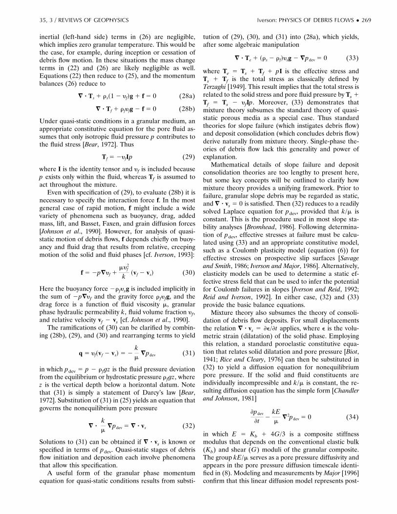
inertial (left-hand side) terms in (26) are negligible,which implies zero granular temperature. This would bethe case, for example, during inception or cessation ofdebris flow motion. In these situations the mass changeterms in (22) and (26) are likely negligible as well.Equations (22) then reduce to (25), and the momentumbalances (26) reduce to

= ? Ts 1 rs~1 2 yf!g 1 f 5 0 (28a)

= ? Tf 1 rfyfg 2 f 5 0 (28b)

Under quasi-static conditions in a granular medium, anappropriate constitutive equation for the pore fluid as-sumes that only isotropic fluid pressure p contributes tothe fluid stress [Bear, 1972]. Thus

Tf 5 2yfIp (29)

where I is the identity tensor and yf is included becausep exists only within the fluid, whereas Tf is assumed toact throughout the mixture.

Even with specification of (29), to evaluate (28b) it isnecessary to specify the interaction force f. In the mostgeneral case of rapid motion, f might include a widevariety of phenomena such as buoyancy, drag, addedmass, lift, and Basset, Faxen, and grain diffusion forces[Johnson et al., 1990]. However, for analysis of quasi-static motion of debris flows, f depends chiefly on buoy-ancy and fluid drag that results from relative, creepingmotion of the solid and fluid phases [cf. Iverson, 1993]:

f 5 2p=yf 1myf

2

k ~vf 2 vs! (30)

Here the buoyancy force 2rfysg is included implicitly inthe sum of 2p=yf and the gravity force rfyfg, and thedrag force is a function of fluid viscosity m, granularphase hydraulic permeability k, fluid volume fraction yf,and relative velocity vf 2 vs [cf. Johnson et al., 1990].

The ramifications of (30) can be clarified by combin-ing (28b), (29), and (30) and rearranging terms to yield

q 5 yf~vf 2 vs! 5 2km

=pdev (31)

in which pdev 5 p 2 rfgz is the fluid pressure deviationfrom the equilibrium or hydrostatic pressure rfgz, wherez is the vertical depth below a horizontal datum. Notethat (31) is simply a statement of Darcy’s law [Bear,1972]. Substitution of (31) in (25) yields an equation thatgoverns the nonequilibrium pore pressure

= ?km

=pdev 5 = ? vs (32)

Solutions to (31) can be obtained if = z vs is known orspecified in terms of pdev. Quasi-static stages of debrisflow initiation and deposition each involve phenomenathat allow this specification.

A useful form of the granular phase momentumequation for quasi-static conditions results from substi-

tution of (29), (30), and (31) into (28a), which yields,after some algebraic manipulation

= ? Te 1 ~rs 2 rf!ysg 2 =pdev 5 0 (33)

where Te 5 Ts 1 Tf 1 pI is the effective stress andTs 1 Tf is the total stress as classically defined byTerzaghi [1949]. This result implies that the total stress isrelated to the solid stress and pore fluid pressure by Ts 1Tf 5 Ts 2 yfIp. Moreover, (33) demonstrates thatmixture theory subsumes the standard theory of quasi-static porous media as a special case. Thus standardtheories for slope failure (which instigates debris flow)and deposit consolidation (which concludes debris flow)derive naturally from mixture theory. Single-phase the-ories of debris flow lack this generality and power ofexplanation.

Mathematical details of slope failure and depositconsolidation theories are too lengthy to present here,but some key concepts will be outlined to clarify howmixture theory provides a unifying framework. Prior tofailure, granular slope debris may be regarded as static,and = z vs 5 0 is satisfied. Then (32) reduces to a readilysolved Laplace equation for pdev, provided that k/m isconstant. This is the procedure used in most slope sta-bility analyses [Bromhead, 1986]. Following determina-tion of pdev, effective stresses at failure must be calcu-lated using (33) and an appropriate constitutive model,such as a Coulomb plasticity model (equation (6)) foreffective stresses on prospective slip surfaces [Savageand Smith, 1986; Iverson and Major, 1986]. Alternatively,elasticity models can be used to determine a static ef-fective stress field that can be used to infer the potentialfor Coulomb failures in slopes [Iverson and Reid, 1992;Reid and Iverson, 1992]. In either case, (32) and (33)provide the basic balance equations.

Mixture theory also subsumes the theory of consoli-dation of debris flow deposits. For small displacementsthe relation = z vs 5 ]e/]t applies, where e is the volu-metric strain (dilatation) of the solid phase. Employingthis relation, a standard poroelastic constitutive equa-tion that relates solid dilatation and pore pressure [Biot,1941; Rice and Cleary, 1976] can then be substituted in(32) to yield a diffusion equation for nonequilibriumpore pressure. If the solid and fluid constituents areindividually incompressible and k/m is constant, the re-sulting diffusion equation has the simple form [Chandlerand Johnson, 1981]

]pdev

]t 2kEm

=2pdev 5 0 (34)

in which E 5 Kb 1 4G/3 is a composite stiffnessmodulus that depends on the conventional elastic bulk(Kb) and shear (G) moduli of the granular composite.The group kE/m serves as a pore pressure diffusivity andappears in the pore pressure diffusion timescale identi-fied in (8). Modeling and measurements by Major [1996]confirm that this linear diffusion model represents post-


depositional consolidation of debris flow deposits rea-sonably well (Figure 13). However, changes in perme-ability and stiffness may produce nonlinear behavior thatis especially important in the early stages of consolida-tion, when the solid grains are loosely packed and themixture undergoes large strains. This nonlinearity isanalyzed in section 8.

6.2. Inertial MotionThe mixture theory approach provides a complete

framework for predicting quasi-static phenomena duringinitiation and deposition of debris flows, but can thetheory represent inertial debris flow motion with non-zero granular temperature? In kinetic theories of drygranular flow, the concept of granular temperature leadsto a balance equation for the fluctuation energy of thesolid grains, which must be satisfied along with momen-tum and mass balances. The physical motivation andinterpretation of granular temperature equations weredescribed by Haff [1983, 1986], and mathematical con-nections of such equations to classical kinetic theorywere established by Jenkins and Savage [1983] and Lun etal. [1984]. A typical form of such an equation is given byCampbell [1990]:

12 rsys@]T/]t 1 vs ? =T# 5 2= ? j 2 Ts:=vs 2 G (35)

wherein T 5 ^v9s2& is the granular temperature, j is the

conductive flux of granular temperature from highlyagitated to less-agitated regions within the flow, Ts:=vs isthe rate of generation of granular temperature via workperformed by the stresses, Ts, and G is the rate ofdegradation of granular temperature into thermody-namic heat as a result of dissipative grain interactions.An important implication of (35) is that grain fluctuationenergy cannot be specified as a simple function of thelocal shear rate and solid volume fraction; instead, gran-ular temperature is a field variable that may depend in acomplicated way on boundary conditions and transportphenomena.

Rigorous application of (35) requires knowledge of adiffusion coefficient for j as well as appropriate bound-ary conditions and constitutive parameters to determineTs and G. For purely collisional flows with identicalspherical grains characterized only by their size (d),density (rs), and coefficient of restitution (e), the nec-essary information can be deduced from kinetic theory(see the review by Campbell [1990]). For flows in whichenduring, frictional grain contacts may play an impor-tant role, the theory is less complete [Anderson andJackson, 1992]. If, in addition, a viscous intergranularfluid is present, satisfactory theory is lacking entirely.However, hueristic analyses indicate that conduction offluid pressure fluctuations that occur if there is nonzerogranular temperature can play an important, perhapsdominant, role in mixture momentum transport whenviscous fluid is present [Jenkins and McTigue, 1990; Mc-Tigue and Jenkins, 1992]. Thus although the effects of

granular temperature on debris flow dynamics are notyet rigorously quantified, they are both theoretically andempirically identifiable. Section 7 provides further in-sight.

A better basis exists for evaluating the dynamic inter-action force f during inertial debris flow motion. Dragarguably constitutes the most significant interactionforce in most solid-fluid mixture flows [Johnson et al.,1990]. Thus the Darcian drag described by (30) mightrepresent the most important interactions in inertial aswell as quasi-static stages of debris flows. Comparison ofthe experimental results of Iverson and LaHusen [1989]with calculations that use the model of Iverson [1993]show that Darcy coupling alone can yield excellent pre-dictions of fluid pressures even when grain Reynoldsnumbers fall well above the Stokes flow limit. Moreover,an analysis by DiFelice [1994] of diverse experimentaldata on fluid drag forces in both dilute and concentratedsuspensions of spheres shows that the total drag dependsstrongly on the solid volume fraction ys but surprisinglyweakly on the grain Reynolds number over the range1022 , NRey , 104 (where NRey depends on the abso-lute value of the relative solid-fluid velocity, vf 2 vs).Thus, as a first approximation, a simple Darcy-dragmodel may be valid for debris flows.

Finally, appropriate boundary conditions as well asconstitutive equations that relate the stresses Tf and Ts

to the velocities vf and vs must in general be specified tosolve the momentum equations (26). Appropriate con-stitutive equations for a Newtonian fluid phase are wellknown, but appropriate equations for the granular phaseare lacking. Although beginnings have been made alongthese lines [e.g., Shen and Ackermann, 1982], rigorousformulations analogous to those for collisional dry grainflows [e.g., Lun et al., 1984] have not been developed [cf.Garcia-Aragon, 1995]. To build insight, the next sectionconsiders solid, fluid, and boundary effects on momen-tum transport from the perspective of elementary me-chanics.

7. GRAIN, FLUID, AND BOUNDARYINTERACTIONS: ANALYTICAL SOLUTIONSFOR IDEALIZED, STEADY FLOW

The balance equations of the preceding section pro-vide a quantitative but rather general picture of debrisflow mixture dynamics. To gain more detailed under-standing, solutions and not merely balance equationsmust be investigated. Although solutions for quasi-staticslope failure and deposit consolidation problems areabundant in the literature, solutions for boundary valueproblems that contain all the dynamic variables in (22),(26), and (35) are unavailable. This section thereforeconsiders primitive forms of the balance equations thatadmit explicit analytical solutions. These solutions clar-ify physical effects of solid-fluid interactions and bound-ary conditions, and they reveal the significance of solid


and fluid velocities normal to the bed, which are ne-glected in most practical models (see section 9). As aby-product, the solutions quantify the shortcomings ofBagnold’s [1954] formulas as constitutive equations fordebris flows. They also indicate that presence of a vis-cous fluid phase reduces the net efficiency of steady,uniform motion of a granular material. This result con-tradicts the observation that viscous fluid enhances de-bris flow efficiency (sections 2 and 3), and thus reveals alimitation of steady state theories; it supports the ideathat debris flows may be fundamentally unsteady phe-nomena.

Guidance for simplifying debris flow mixture theorycomes from work on closely related granular flows. Forexample, Anderson and Jackson [1992] have shown thatin steady, uniform, gravity-driven flows of dry grains thatinteract through both collisions and friction, significantvariations in granular temperature, solid volume frac-tion, and mean grain velocity commonly occur only nearthe bed; grains far from the bed “lock” and translate asa rigid body if there is much dissipation and little con-duction of granular temperature into the flow interior.Jenkins and Askari [1994] have exploited this fact toanalyze the dynamics of unsteady, dry, granular flowswith nonzero granular temperatures concentrated in athin basal shear layer. Similar locking behavior neces-sarily occurs in debris flows during initiation and depo-sition and appears to occur when “rigid” plugs formduring sustained debris flow motion [Johnson, 1984].

With this background, consider a hypothetical steady,uniform debris flow moving down a rough, impermeable,fixed bed of infinite extent and uniform inclination. Bydefinition, no variation of any quantity occurs in direc-tions parallel or transverse to the slope (Figure 17). Theflow translates with velocity vx and for simplicity hasvelocity fluctuations v9 with only y components. A mov-ing coordinate x9 5 x 2 vxt that translates with thesteady flow in the x direction provides a convenientframe of reference. Shearing occurs only between thebed and a single layer of grains and fluid. A thick, lockedlayer of grains that moves downslope as a rigid bodyoverlies the shearing layer. The goal is to understandhow momentum communicated by the shear layer to thelocked layer and bed is influenced by the shear rate andmaterial properties such as solid and fluid densities,grain friction and restitution coefficients, and fluid vis-cosity. This understanding may then be extrapolated tomore general cases where many layers of grains shearpast one another.

Substantial simplification can be achieved with littlesacrifice of relevance if the fluctuating motions of theshearing and locked layers occupy specified domains iny. It is convenient to define the boundary between thesedomains as y 5 0. Thus in the coordinate system ( x9, y),assume that a shear layer grain with characteristic diam-eter d and mass m2 moves only in the domain betweeny 5 0 and y 5 2d 2 s, where s can be viewed as themean free path of grain oscillation. The overlying locked

layer of grains, of collective mass m1 (..m2), movesonly between y 5 0 and the upper flow surface (Figure17). Interactions of the shear layer and locked layeroccur exclusively at y 5 0. No fluid or solid mass movesbetween the sheared and locked domains, and grains inboth domains are rigid. These simplifications reduce thecontinuum-mixture problem to a discrete two-bodyproblem that entails explicit analysis of momentum ex-change at the domain boundary. The analysis parallelsthat of Bagnold [1954] but differs by including the effectsof gravity, a free surface, and dissimilar masses m1 andm2, all of which exist in debris flows.

The idealization described above simplifies the gov-erning equations substantially. Grain fluctuation energyis conducted from the basal shear layer to the lockedlayer by momentum exchange between the layers, butthe time-averaged conduction does not change the gran-ular temperature of either layer. Thus the fluctuationenergy equation (35) becomes unnecessary; terms onboth the left and right sides of (35) sum to zero for boththe shear layer and the locked layer. Furthermore, themass balance equations (22) applicable in each domainare satisfied trivially, and the x components of the mo-mentum equations (26) reduce to simple steady statebalances. The momentum equations for motion of thesolids and fluid in the y direction reduce to

Figure 17. Schematic vertical cross section of a representa-tive segment of an idealized debris flow (and translating coor-dinate system ( x9, y)) that move downstream with constantvelocity vx. Within the segment a single grain of mass m2

exchanges momentum with the bed and the overlying grains,which have collective mass m1. All momentum transfer andunsteady motion occur in the y direction. The fluctuatingmotion of m2 is restricted to a vertical domain defined by thecharacteristic grain diameter d and mean free path s. All grainsare surrounded by fluid less dense than the grains. Gravity actsin the 2y direction.


rsys

dvdt 5 ys~rs 2 rf! gy 2

myf

k v (36a)

0 5 2dpd y 1 rfgy 1

myf

k v (36b)

in which v designates the solid fluctuation velocity in they direction and gy is the y component of g. (Here primesand subscripts are omitted on v to simplify the notation.)No term involving the solid stress Ts appears in (36a)because the solid masses in each domain are treated asdiscrete bodies. Instead, the time-integrated grain iner-tia force * rsys(dv/dt) dt communicated by impulses atdomain boundaries predicts the time-averaged solid nor-mal stress and obviates the need for a continuum stressterm [cf. Iverson, 1993]. In addition, (36b) lacks fluidacceleration terms. This omission is justified if the di-mensionless group myf

2d/kravx (where ra is the added-mass density of solid grains accelerating through adja-cent fluid) has a value substantially greater than 1, whichindicates that solid-fluid interaction forces are domi-nated by viscous rather than inertial effects, a conditionprobably satisfied in many debris flows [Iverson, 1993].Furthermore, (36a) and (36b) are only partly coupled;(36a) can be solved explicitly for the solid fluctuationvelocity, which can then be input to (36b) to solve for thepore fluid pressure distribution. The pore fluid pressuregradient dp/d y is negative under static conditions (v 50) because y is reckoned positive upward and gy isnegative; dp/d y increases when the solid fluctuationvelocity v is positive and decreases when v is negative.However, (36b) shows that there is no tendency for netexcess fluid pressures to develop if a net upward ordownward solid velocity is absent. Fluid pressures thatfluctuate so that the time-averaged excess pressure iszero have been measured in laboratory experiments withidealized debris flow mixtures [Iverson and LaHusen,1989] and predicted with a model similar to (36) thatcouples inertial grain motion to pore pressure diffusion[Iverson, 1993].

Solutions of the y direction momentum equation forthe solids (equation (36a)) hold the key to understand-ing this idealized debris flow and can be described best ifthe equation is first recast as

d2udt2 1 A

dudt 5 B (37a)

in which u 5 * v dt is the solid displacement and A andB are defined by

A 5yfm

ysrsk(37b)

B 5 S1 2rf

rsD gy (37c)

Note that B is generally negative because gy is negativeand rf , rs, but B 5 0 if the solid grains are neutrally

buoyant (the case of Bagnold [1954]). If the fluid isinviscid or absent, A 5 0 as well.

Equation (37a) has the solution

u 5 2C1

A exp ~2At! 1BA t 1 C2 (38)

in which C1 and C2 are constants determined by initialconditions. If B 5 0, this solution lacks the second term,but if A 5 0 (indicating an inviscid fluid), an entirelydifferent solution applies:

u 512 Bt2 1 C1t 1 C2 (39)

It is instructive to examine first the predictions of thissolution for A 5 0 and then to compare them withpredictions of the more strongly nonlinear solution (38).

7.1. Inviscid Case (A 5 0)Initial conditions determine the values of C1 and C2

needed to complete the inviscid solution (39) for themotion of grain masses m1 and m2. For the upper,locked mass (m1), appropriate initial conditions are

u~0! 5 0 (40a)

v~0! 5 du/dt~0! 5 v0 (40b)

which give C1 5 v0, C2 5 0, and the solutions forposition and velocity

u 512 Bt2 1 v0t (41a)

v 5 Bt 1 v0 (41b)

These are simple ballistic trajectory equations for theoscillating motion of m1, which is sustained by impulsesfrom m2. From (41a) it is easy to see that m1 returns toits initial position, u 5 0, after a time tcycle:

tcycle 5 22~v0/B! (42)

At t 5 tcycle, m1 collides with m2, and then repeats itstrajectory.

The oscillations of m2 are more complicated, becausethey must supply enough momentum to sustain the os-cillations of m1 and also satisfy (39), (42), and a condi-tion for interaction with the bed, which includes bothcollisional dissipation and frictional dissipation due toslip at the bed. Thus for m2, paired evaluations of (39)are required, one for upward motion and one for down-ward motion. Paired initial conditions are also needed,which can be written in terms of the grain position u;downward bound velocity vdown; upward bound velocityvup; arrival time at the top of the domain boundary, tup;and arrival time at the bottom of the domain boundary,tdown. The initial conditions are

Downward bound

u~tup! 5 0 (43a)


vdown~tup! 5 v0down 5 2evup~tup! (43b)

Upward bound

u~tdown! 5 2s (43c)

vup~tdown! 5 v0up 5 2evdown~tdown! 1 c (43d)

in which v0up and v0down are the initial values of vup andvdown, respectively, and c is a very important quantitywith dimensions of velocity.

Values of c measure the net conversion of transla-tional momentum m2vx into fluctuation momentum m2vthat results from interaction of m2 with the rough bed(Figure 18). Grain fluctuation energy generated byworking of the bed shear stress minus grain energy lostto inelastic collisions and bed friction equals 1

2 m2c2.Because grain interactions with the bed and one anothergenerally dissipate energy, a positive value of c is nec-essary to conduct fluctuation energy away from the bedand prevent the mass from locking frictionally.

The restitution coefficient e in (43b) applies to thecollision of the shear layer grain m2 and the overlyingmass m1. An exact analysis of the collision shows that eshould be replaced by an effective coefficient of restitu-tion which differs slightly from the true coefficient (Ap-pendix A). However, for the condition m1 .. m2 as-sumed here, the difference between the effective andtrue values of e is negligible.

Evaluation of (39) for the initial conditions (43) yieldsupward bound and downward bound solutions for theposition and velocity of m2, which at times tdown and tupreduce to

12 Btdown

2 1 v0downtdown 5 2s (44a)

12 Btup

2 1 v0uptup 5 s (44b)

Btdown 1 v0down 5 21e v0up 1

c

e (44c)

Btup 1 v0up 5 21e v0down (44d)

These four equations contain six unknowns, tup, tdown,v0up, v0down, s and c; therefore two additional equationsare required for closure. Constraints on collisions be-tween m2 and m1 provide the necessary equations. Col-lisions occur at time tcycle, as defined by (42), so it isnecessary that

tup 1 tdown 5 tcycle 5 22~v0/B! (45)

Moreover, collisions must conserve momentum, whichfor m1 .. m2 requires (Appendix A)

v0down 52v0m1~1 1 e! 1 ~m2 2 em1!@2v0down~1/e!#

m1 1 m2(46)

Thus (44), (45), and (46) form a closed, slightly nonlin-ear set of equations that can be solved explicitly.

Solutions of the set (44)–(46) yield key quantitiessuch as s and c, and also facilitate evaluation of thegranular temperature, granular stress and Bagnold’s[1954] “dispersive pressure.” The exact solutions arealgebraically cumbersome and are stated in Appendix Bas equations (B1)–(B6). Valid approximations of (B1)–(B6) can be obtained by further exploiting the assump-tion m2/m1 ,, 1. As m2/m1 3 0, the exact expressionfor c (equation (B6)) reduces to

c 5 v0~m1/m2!~1 2 e2! (47a)

Substituting (47a) into (B1)–(B5) then yields the approx-imations

tup 5 21B v0

2e1 1 e (47b)

tdown 5 tup/e (47c)

v0down 5 2~m1/m2!ev0 (47d)

v0up 5 v0S 2e1 1 e 1

m1

m2D (47e)

s 522v0

2eB~1 1 e! F 1

1 1 e 1m1

m2G (47f )

The approximation error is zero for all values of m1/m2if e 5 1 but grows as e 3 0.

The simple equations (47a)–(47f) describe the essen-tial physics of the inviscid case; Table 7 lists some nu-merical values that satisfy the equations. The tabulatedvalues demonstrate the following effects: (1) If v0, B, e,and m2 are held fixed, increased grain fluctuation speedsand increased mean free paths are required to sustainmotion if the overburden mass m1 is increased. Collisionfrequencies and tcycle remain constant, but more fluctu-ation energy is required to support the increased over-burden and prevent the entire mass from locking. (2) Ife 5 1, then tup 5 tdown, and mean fluctuation speeds areidentical in the upward and downward directions; no

Figure 18. Schematic diagram depicting conversion of slopeparallel translation velocity into slope normal fluctuation ve-locity as a grain interacts with a rough bed. The slope normalvelocity generated minus velocity lost due to frictional andcollisional energy dissipation determines c.


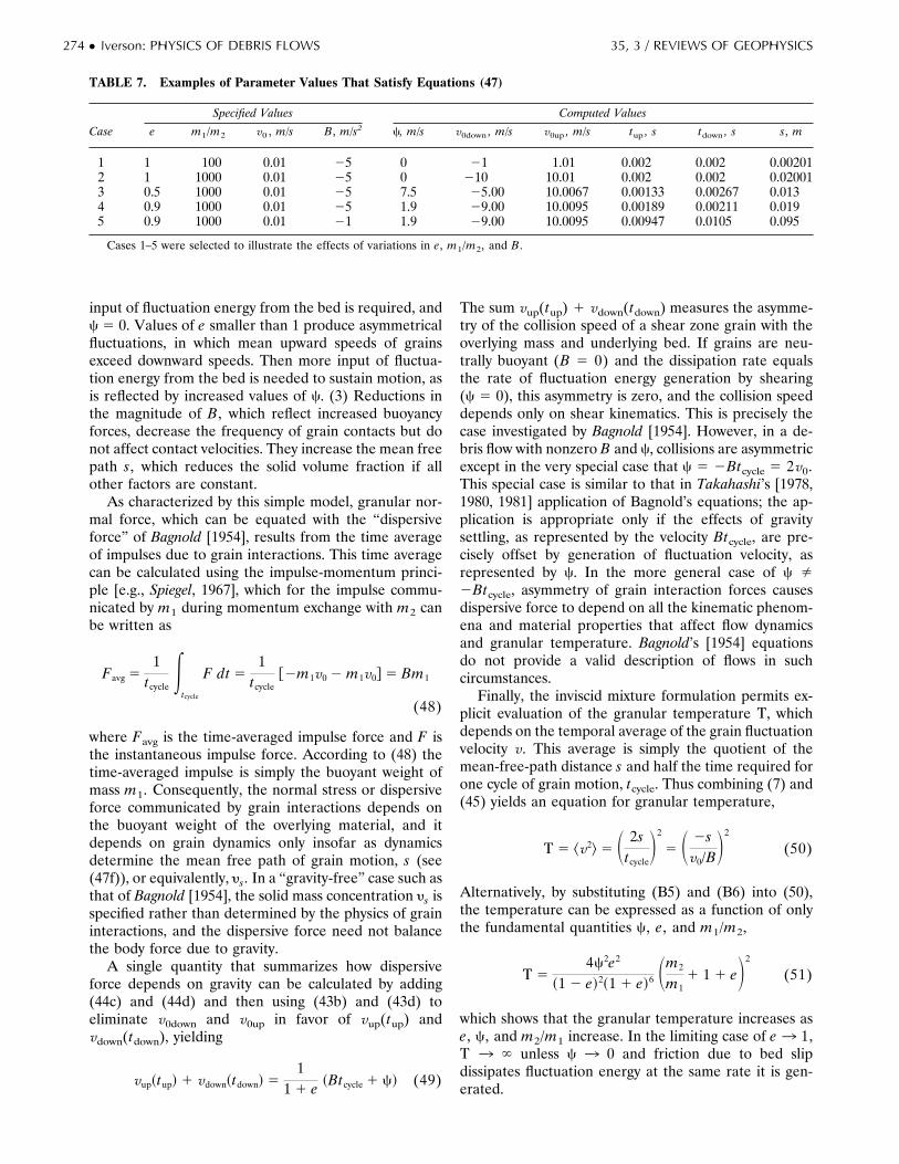
input of fluctuation energy from the bed is required, andc 5 0. Values of e smaller than 1 produce asymmetricalfluctuations, in which mean upward speeds of grainsexceed downward speeds. Then more input of fluctua-tion energy from the bed is needed to sustain motion, asis reflected by increased values of c. (3) Reductions inthe magnitude of B, which reflect increased buoyancyforces, decrease the frequency of grain contacts but donot affect contact velocities. They increase the mean freepath s, which reduces the solid volume fraction if allother factors are constant.

As characterized by this simple model, granular nor-mal force, which can be equated with the “dispersiveforce” of Bagnold [1954], results from the time averageof impulses due to grain interactions. This time averagecan be calculated using the impulse-momentum princi-ple [e.g., Spiegel, 1967], which for the impulse commu-nicated by m1 during momentum exchange with m2 canbe written as

Favg 51

tcycleE

tcycle

F dt 51

tcycle@2m1v0 2 m1v0# 5 Bm1

(48)

where Favg is the time-averaged impulse force and F isthe instantaneous impulse force. According to (48) thetime-averaged impulse is simply the buoyant weight ofmass m1. Consequently, the normal stress or dispersiveforce communicated by grain interactions depends onthe buoyant weight of the overlying material, and itdepends on grain dynamics only insofar as dynamicsdetermine the mean free path of grain motion, s (see(47f)), or equivalently, ys. In a “gravity-free” case such asthat of Bagnold [1954], the solid mass concentration ys isspecified rather than determined by the physics of graininteractions, and the dispersive force need not balancethe body force due to gravity.

A single quantity that summarizes how dispersiveforce depends on gravity can be calculated by adding(44c) and (44d) and then using (43b) and (43d) toeliminate v0down and v0up in favor of vup(tup) andvdown(tdown), yielding

vup~tup! 1 vdown~tdown! 51

1 1 e ~Btcycle 1 c! (49)

The sum vup(tup) 1 vdown(tdown) measures the asymme-try of the collision speed of a shear zone grain with theoverlying mass and underlying bed. If grains are neu-trally buoyant (B 5 0) and the dissipation rate equalsthe rate of fluctuation energy generation by shearing(c 5 0), this asymmetry is zero, and the collision speeddepends only on shear kinematics. This is precisely thecase investigated by Bagnold [1954]. However, in a de-bris flow with nonzero B and c, collisions are asymmetricexcept in the very special case that c 5 2Btcycle 5 2v0.This special case is similar to that in Takahashi’s [1978,1980, 1981] application of Bagnold’s equations; the ap-plication is appropriate only if the effects of gravitysettling, as represented by the velocity Btcycle, are pre-cisely offset by generation of fluctuation velocity, asrepresented by c. In the more general case of c Þ2Btcycle, asymmetry of grain interaction forces causesdispersive force to depend on all the kinematic phenom-ena and material properties that affect flow dynamicsand granular temperature. Bagnold’s [1954] equationsdo not provide a valid description of flows in suchcircumstances.

Finally, the inviscid mixture formulation permits ex-plicit evaluation of the granular temperature T, whichdepends on the temporal average of the grain fluctuationvelocity v. This average is simply the quotient of themean-free-path distance s and half the time required forone cycle of grain motion, tcycle. Thus combining (7) and(45) yields an equation for granular temperature,

T 5 ^v2& 5 S 2stcycle

D2

5 S 2sv0/B

D2

(50)

Alternatively, by substituting (B5) and (B6) into (50),the temperature can be expressed as a function of onlythe fundamental quantities c, e, and m1/m2,

T 54c2e2

~1 2 e!2~1 1 e!6 Sm2

m11 1 1 eD2

(51)

which shows that the granular temperature increases ase, c, and m2/m1 increase. In the limiting case of e 3 1,T 3 ` unless c 3 0 and friction due to bed slipdissipates fluctuation energy at the same rate it is gen-erated.

TABLE 7. Examples of Parameter Values That Satisfy Equations (47)

Case

Specified Values Computed Values

e m1/m2 v0 , m/s B, m/s2 c, m/s v0down , m/s v0up , m/s tup , s tdown , s s, m

1 1 100 0.01 25 0 21 1.01 0.002 0.002 0.002012 1 1000 0.01 25 0 210 10.01 0.002 0.002 0.020013 0.5 1000 0.01 25 7.5 25.00 10.0067 0.00133 0.00267 0.0134 0.9 1000 0.01 25 1.9 29.00 10.0095 0.00189 0.00211 0.0195 0.9 1000 0.01 21 1.9 29.00 10.0095 0.00947 0.0105 0.095

Cases 1–5 were selected to illustrate the effects of variations in e, m1/m2, and B.


7.2. Viscous Case (A > 0)The viscous term A in the equation of motion (37a)

adds mathematical complexity that reflects the physicalcomplexity of debris flows. With A . 0, complete ana-lytical results analogous to (47) cannot easily be at-tained, but quantitative inferences about the role ofviscous intergranular fluid can nonetheless be drawn.

The appropriate initial conditions for the viscous caseare the same as for the inviscid case. For the rigidlylocked upper mass m1, substitution of (40) and (43) in(38) leads to the position and velocity solutions

u 5B/A 2 v0

A @exp ~2At! 2 1#] 1BA t (52a)

v 5 ~v0 2 B/A! @exp ~2At!# 1 B/A (52b)

Like the solutions for the inviscid case (41), these equa-tions describe ballistic paths, but they differ by includingthe effects of viscous drag. An important special case of(52b) occurs when At is large enough that exp (2At) 30; then v 5 B/A is a good approximation, which indi-cates that viscous and gravity forces balance and thatsolid grains descend at their terminal velocity. This iscomparable to the settling velocity described in section 3as a basis for distinguishing grains that act as discretesolids from those suspended as part of the fluid.

Further effects of viscous drag can be evaluated bynoting that at time t 5 tcycle, the mass m1 returns to itsoriginal position, u 5 0. Using these values in (52a)yields

exp ~2Atcycle! 5Btcycle

v0 2 B/A 1 1 (53)

and substituting this result into (52b) yields the velocityof m1 at time tcycle,

v~tcycle! 5 Btcycle 1 v0 (54)

This equation matches the analogous equation for theinviscid case, (41b).

The fact that (54) applies in both the viscous andinviscid cases has significant implications, which are clar-ified by comparing viscous and inviscid mixtures movingat the same rate and undergoing similar internal motion.A reasonable criterion for identifying similar internalmotion focuses on the momentum exchanged duringcollision of m1 and m2. This momentum exchange, de-scribed by (46), is the only facet of internal motion thatcan be characterized independently of viscosity; thussimilar flows can be regarded as those for which vx isidentical and the values of m1, m2, e, v0down, v0 in (46)are identical. If v0 is identical in the viscous and inviscidcases, then the magnitude of v(tcycle) must be smaller inthe viscous case because m1 dissipates energy while itdescribes its ballistic trajectory in the viscous case, butnot in the inviscid case. Thus (54) demonstrates that

tcycle~viscous! , tcycle~inviscid! (55)

Consequently, increased viscosity reduces the averagefluctuation velocity of m1 but increases the frequency ofcollisions between m1 and m2, implying that the meanfree path s of m1 is reduced by the presence of viscousfluid. In turn, this result demonstrates that the viscousfluid decreases the granular temperature, as is expressedby (42) and (43). Reduction of granular temperatureoccurs because some of the grain fluctuation energy isconverted to fluid pressure energy, which involves dissi-pative viscous forces.

If viscous forces dissipate energy, how does viscousfluid enhance debris flow efficiency? This question lies atthe heart of debris flow physics. Viscosity causes grainsto interact less energetically (with commensurately lessdissipation) but more frequently, so the effect of viscos-ity on net dissipation due to grain interactions appearsambiguous. The issue can be clarified by assessing therate of conversion of downslope translational momen-tum to grain fluctuation momentum that is required tosustain steady motion. To do so, an explicit expressionfor c/tcycle must be obtained. This requires repetition ofthe steps used to obtain (44a)–(44d) for the shear zonegrain m2 in the inviscid case, which produces analogousexpressions for the viscous case:

B/A 2 v0down

A @exp ~2Atdown! 2 1# 1BA tdown 5 2s

(56a)

B/A 2 v0up

A @exp ~2Atup! 2 1# 1BA tup 5 s (56b)

~v0down 2 B/A! exp ~2Atdown! 1 B/A 5 21e v0up 1

c

e

(56c)

~v0up 2 B/A! exp ~2Atup! 1 B/A 5 21e v0down (56d)

In conjunction with (45) and (46), these four equationsform a set of six equations in six unknowns, whichdetermine the motion of m2. This strongly nonlinear setdoes not admit simple, explicit solutions, but it doesyield useful information. Expressions for exp (2Atup)and exp (2Atdown) can be readily obtained from (56c)and (56d), and these can substituted into (56a) and (56b)to yield

~1/e!v0down 1 v0up 1 Btup 5 sA (57a)

~1/e!v0up 1 v0down 1 Btdown 2 c/e 5 2sA (57b)

Addition of these two equations produces a simple andimportant result: an equation identical to (41) derivedfor the inviscid case. Combination of (41) with (43b) or(43d) and rearrangement of terms yields alternative ex-pressions for c/tcycle, one based on upward bound grainvelocities from takeoff (v0up) to impact (vup(tup)) andone based on analogous downward bound velocities:


c

tcycle5 2e

~1 1 e!

tcycleFvup~tup! 2

1e v0upG 2 eB (58a)

c

tcycle5

1 1 etcycle

Fvdown~tdown! 21e v0downG 2 B (58b)

For both the viscous and inviscid cases, equations (58)quantify the rate of momentum conversion per unit massneeded to sustain steady motion. Terms on the right-hand sides of (58a) and (58b) distinguish the effects offluid density (represented by B, which has a negativevalue) from those of viscosity. Increases in fluid densitycause B 3 0, and this decreases the rate of momentumconversion c/tcycle required to sustain steady motion.

Effects of viscosity enter (58a) and (58b) in a morecomplicated manner, through both tcycle and the grainvelocity terms in brackets. Increased viscosity decreasestcycle and hence tends to increase c/tcycle. In (58a) theterm in brackets must be negative because v0up mustexceed vup(tup) unless there is no viscosity and no effec-tive gravity ( A 5 0 and B 5 0). This shows that c/tcycleis positive unless A 5 0 and B 5 0. In (58b), however,the term in brackets can be either positive or negative,depending on whether the downward bound takeoffvelocity v0down exceeds the terminal velocity inferredfrom (56c), B/A. If v0down exceeds the terminal fallvelocity, then the grain decelerates as it descends towardthe bed, the term in brackets in (58b) is positive, and thevalue of c/tcycle increases. However, if v0down is less thanthe terminal velocity, then the grain accelerates as it

moves toward the bed, the term in brackets in (58b) isnegative, c/tcycle decreases, and some energy savings areaccrued. The effect is most pronounced for large grainsthat have large terminal velocities, and it disappears asgrain size diminishes. Moreover, the effect can occuronly if e , 1, for equating (58a) and (58b) for the specialcase e 5 1 leads to

2@vup~tup! 2 v0up# 5 @vdown~tdown! 2 v0down# (59)

which shows that the term in brackets in (58b) must bepositive if e 5 1. Thus only if grains are sufficiently large(i.e., have sufficiently large terminal velocities) can vis-cosity enhance efficiency, and this effect occurs only asgrains move toward the bed. Figure 19 summarizes pic-torially the various possibilities for energy savings and lossduring grain velocity fluctuations for viscous and inviscidcases with e 5 1 and e , 1. In all cases it is evident thatthe net effect of viscosity is increased dissipation.

The preceding analysis shows that viscous mediationof dissipative grain interactions cannot be expected toenhance the net efficiency of steady debris flow. Thisseems to contradict the most basic observation of debrisflow behavior, that the interstitial liquid phase enhancesnet mobility (see section 2). However, the analysis alsoshows that increases in buoyancy (expressed by dimin-ished magnitudes of B) can enhance efficiency. Indeed,as B 3 0, grain contact forces due to gravity diminish,and grain collision forces are increasingly buffered byviscosity. Pore fluid pressures that exceed hydrostatic

Figure 19. Pictorial summary of relative fluctuation velocities of grain m2 during one cycle of vertical motionin mixtures of elastic (e 5 1) and inelastic (e , 1) grains with viscous and inviscid fluids. Lengths of arrowsdepict the relative speeds of m2: v0up is the initial upward velocity of m2 as it departs the bed, and vup(tup)is its upward velocity just before it contacts the overlying mass of grains, m1; v0down is the initial downwardvelocity of m2 just after it contacts m1, and vdown(tdown) is its downward velocity just before it contacts the bed.Dotted lines at the end of a motion cycle denote the deficit in fluctuation velocity (due to energy dissipation),which must be resupplied by c to sustain the fluctuating motion. B/A is the terminal descent velocity of m2

in a viscous fluid.


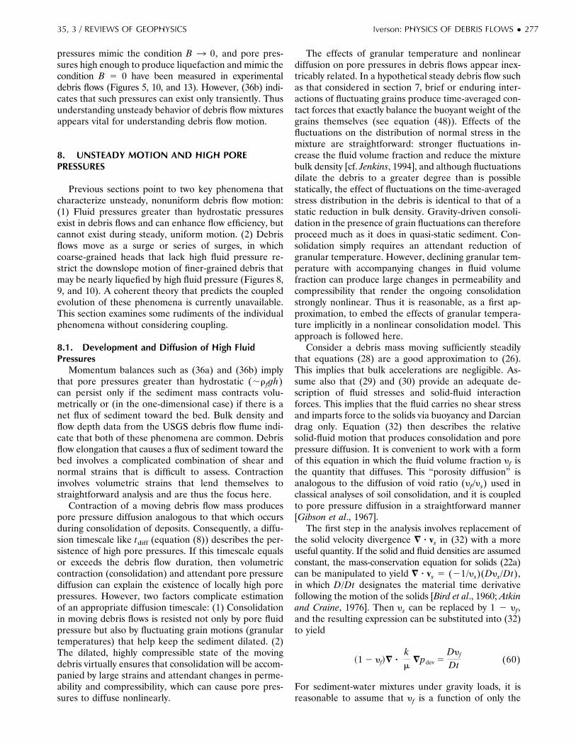
pressures mimic the condition B 3 0, and pore pres-sures high enough to produce liquefaction and mimic thecondition B 5 0 have been measured in experimentaldebris flows (Figures 5, 10, and 13). However, (36b) indi-cates that such pressures can exist only transiently. Thusunderstanding unsteady behavior of debris flow mixturesappears vital for understanding debris flow motion.

8. UNSTEADY MOTION AND HIGH POREPRESSURES

Previous sections point to two key phenomena thatcharacterize unsteady, nonuniform debris flow motion:(1) Fluid pressures greater than hydrostatic pressuresexist in debris flows and can enhance flow efficiency, butcannot exist during steady, uniform motion. (2) Debrisflows move as a surge or series of surges, in whichcoarse-grained heads that lack high fluid pressure re-strict the downslope motion of finer-grained debris thatmay be nearly liquefied by high fluid pressure (Figures 8,9, and 10). A coherent theory that predicts the coupledevolution of these phenomena is currently unavailable.This section examines some rudiments of the individualphenomena without considering coupling.

8.1. Development and Diffusion of High FluidPressures

Momentum balances such as (36a) and (36b) implythat pore pressures greater than hydrostatic (;rfgh)can persist only if the sediment mass contracts volu-metrically or (in the one-dimensional case) if there is anet flux of sediment toward the bed. Bulk density andflow depth data from the USGS debris flow flume indi-cate that both of these phenomena are common. Debrisflow elongation that causes a flux of sediment toward thebed involves a complicated combination of shear andnormal strains that is difficult to assess. Contractioninvolves volumetric strains that lend themselves tostraightforward analysis and are thus the focus here.

Contraction of a moving debris flow mass producespore pressure diffusion analogous to that which occursduring consolidation of deposits. Consequently, a diffu-sion timescale like tdiff (equation (8)) describes the per-sistence of high pore pressures. If this timescale equalsor exceeds the debris flow duration, then volumetriccontraction (consolidation) and attendant pore pressurediffusion can explain the existence of locally high porepressures. However, two factors complicate estimationof an appropriate diffusion timescale: (1) Consolidationin moving debris flows is resisted not only by pore fluidpressure but also by fluctuating grain motions (granulartemperatures) that help keep the sediment dilated. (2)The dilated, highly compressible state of the movingdebris virtually ensures that consolidation will be accom-panied by large strains and attendant changes in perme-ability and compressibility, which can cause pore pres-sures to diffuse nonlinearly.

The effects of granular temperature and nonlineardiffusion on pore pressures in debris flows appear inex-tricably related. In a hypothetical steady debris flow suchas that considered in section 7, brief or enduring inter-actions of fluctuating grains produce time-averaged con-tact forces that exactly balance the buoyant weight of thegrains themselves (see equation (48)). Effects of thefluctuations on the distribution of normal stress in themixture are straightforward: stronger fluctuations in-crease the fluid volume fraction and reduce the mixturebulk density [cf. Jenkins, 1994], and although fluctuationsdilate the debris to a greater degree than is possiblestatically, the effect of fluctuations on the time-averagedstress distribution in the debris is identical to that of astatic reduction in bulk density. Gravity-driven consoli-dation in the presence of grain fluctuations can thereforeproceed much as it does in quasi-static sediment. Con-solidation simply requires an attendant reduction ofgranular temperature. However, declining granular tem-perature with accompanying changes in fluid volumefraction can produce large changes in permeability andcompressibility that render the ongoing consolidationstrongly nonlinear. Thus it is reasonable, as a first ap-proximation, to embed the effects of granular tempera-ture implicitly in a nonlinear consolidation model. Thisapproach is followed here.

Consider a debris mass moving sufficiently steadilythat equations (28) are a good approximation to (26).This implies that bulk accelerations are negligible. As-sume also that (29) and (30) provide an adequate de-scription of fluid stresses and solid-fluid interactionforces. This implies that the fluid carries no shear stressand imparts force to the solids via buoyancy and Darciandrag only. Equation (32) then describes the relativesolid-fluid motion that produces consolidation and porepressure diffusion. It is convenient to work with a formof this equation in which the fluid volume fraction yf isthe quantity that diffuses. This “porosity diffusion” isanalogous to the diffusion of void ratio (yf/ys) used inclassical analyses of soil consolidation, and it is coupledto pore pressure diffusion in a straightforward manner[Gibson et al., 1967].

The first step in the analysis involves replacement ofthe solid velocity divergence = z vs in (32) with a moreuseful quantity. If the solid and fluid densities are assumedconstant, the mass-conservation equation for solids (22a)can be manipulated to yield = z vs 5 (21/ys)(Dys/Dt),in which D/Dt designates the material time derivativefollowing the motion of the solids [Bird et al., 1960; Atkinand Craine, 1976]. Then ys can be replaced by 1 2 yf,and the resulting expression can be substituted into (32)to yield

~1 2 yf!= ?km

=pdev 5Dyf

Dt (60)

For sediment-water mixtures under gravity loads, it isreasonable to assume that yf is a function of only the


effective stress, and thus of pdev. Then application of thechain rule, =pdev 5 (]pdev/]yf)=yf, allows (60) to berecast as

= ?k~1 2 yf!

m

]pdev

]yf=yf 5

Dyf

Dt (61)

in which the factor ]pdev/]yf plays the role of a stiffnessmodulus (reciprocal compressibility) of the mixture.

The conventional expression for the compressibility Cof sediment-water mixtures describes the change inpore volume yf due to changes in effective stress, C 52]yf/](s 2 p). (Here s is the total normal stress,defined as positive in compression, which is related tothe stresses in section 6 by s 5 21

3 (tr Ts 1 tr Tf), wheretr denotes the trace of the tensor.) For large strains, areasonable postulate is that this compressibility variesinversely with the effective stress,

C < k/~s 2 p! (62)

where k is a positive constant typically smaller than 1.Relationship (62) implies that the mixture grows pro-gressively less compressible as consolidation proceedsand effective stress increases. Combining the definitionC 5 2]yf/](s 2 p) with (62) and integrating theresulting equation shows that (62) also implies that thefluid volume fraction (porosity) declines logarithmicallyas effective stress increases:

yf 5 yf 0 2 k ln u~s 2 p!/~s 2 p!0u (63)

in which yf 0 and (s 2 p)0 are characteristic values of thefluid volume fraction and effective stress that derivefrom the stipulation that yf 5 yf0 when s 2 p 5 (s 2 p)0.Data plotted in Figure 20 indicate that a logarithmicrelationship such as (63) describes the volume changebehavior of a variety of soils, slurries, and debris flow

mixtures reasonably well [cf. Lambe and Whitman, 1979,p. 320; Been and Sills, 1981].

For problems of gravitational consolidation underconstant load, the compressibility ]yf/]pdev in (61)matches the compressibility C 5 2]yf/](s 2 p) definedin terms of effective stress. This is apparent from thedefinition of effective stress, which can be written as

s 2 p 5 s 2 rfgz 2 pdev (64)

where the second term on the right-hand side is thehydrostatic component of the pore pressure, which re-mains constant. For estimation of consolidation behav-ior, the total stress s can also be regarded as constantbecause the total stress changes little in comparison withthe pore pressure during consolidation. Thus ](s 2 p) '](2pdev), and the compressibility estimate defined by(62) can be substituted into (61), yielding

= ?k~1 2 yf!

mC =yf <Dyf

Dt (65)

This may be interpreted as an advection-diffusion equa-tion for yf, in which the advection velocity is the velocityvs of the reference frame for the material time derivativeDyf/Dt [Iverson, 1993] [cf. Atkin and Craine, 1976]. Thusit is possible to exploit the fact that in a coordinatesystem that moves with velocity vs, (65) transforms intoa standard diffusion equation that is readily solved [Iver-son, 1993] [cf. Ogata, 1970].

The expression k(1 2 yf)/mC, which plays the role ofthe hydraulic diffusivity in (65), can be used to under-stand the character of nonlinear consolidation and esti-mate the timescale of nonlinear pore pressure diffusion.The expression can be written in a more explicit form bynoting that the permeability of most sediment mixtures,including debris flow mixtures (Figure 6), is an exponen-tial function of porosity or fluid volume fraction, k 5 k0exp (ayf) [cf. Lambe and Whitman, 1979, p. 286; Beenand Sills, 1981]. Use of this expression and (62) leads toan estimate of the hydraulic diffusivity Dh,

Dh 5k~1 2 yf!

mC 5k0~1 2 yf!~s 2 p!

kmexp ~ayf! (66)

which shows that the diffusivity is also an exponentialfunction of fluid volume fraction. The implications of(66) can be clarified by noting that (63) can be used torewrite the exponential function as

exp ~ayf! 5 exp @a~yf0 2 k ln u~s 2 p!/~s 2 p!0u!#(67)

5 exp ~ayf0!/@~s 2 p!/~s 2 p!0#ak

Substituting (67) into (66) then yields

Dh 5~1 2 yf!k0 exp ~ayf0!

mk~s 2 p!0

ak~s 2 p!12ak (68)

An obvious implication of the last factor in (68) is thatthe character of pore pressure diffusion depends on

Figure 20. Data trends illustrating the approximate propor-tionality between fluid volume fraction (porosity) and thelogarithm of effective stress in various soils and suspensions.Numbers identify data source: 1, Lambe and Whitman [1979];2, Been and Sills [1981]; 3, Major [1996].


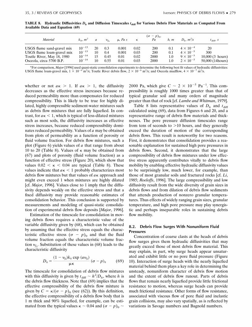
whether or not ak . 1. If ak . 1, the diffusivitydecreases as the effective stress increases because re-duced permeability more than compensates for reducedcompressibility. This is likely to be true for highly di-lated, highly compressible sediment-water mixtures suchas debris flow mixtures that are fully liquefied. In con-trast, for ak , 1, which is typical of less-dilated mixturessuch as most soils, the diffusivity increases as effectivestress increases, because reduced compressibility domi-nates reduced permeability. Values of a may be obtainedfrom plots of permeability as a function of porosity orfluid volume fraction. For debris flow mixtures, such aplot (Figure 6) yields values of a that range from about10 to 20 (Table 8). Values of k may be obtained from(67) and plots of porosity (fluid volume fraction) as afunction of effective stress (Figure 20), which show thatvalues 0.02 , k , 0.04 are typical (Table 8). Thesevalues indicate that ak , 1 probably characterizes mostdebris flow mixtures but that values of ak approach andmight even exceed 1 when mixtures are highly dilated[cf. Major, 1996]. Values close to 1 imply that the diffu-sivity depends weakly on the effective stress and that afixed diffusivity may provide reasonable estimates ofconsolidation behavior. This conclusion is supported bymeasurements and modeling of quasi-static consolida-tion of experimental debris flow deposits [Major, 1996].

Estimation of the timescale for consolidation in mov-ing debris flows requires a characteristic value of thevariable diffusivity given by (68), which can be obtainedby assuming that the effective stress equals the charac-teristic effective stress (s 2 p)0 and that the fluidvolume fraction equals the characteristic volume frac-tion yf0

. Substitution of these values in (68) leads to thecharacteristic diffusivity

Dh 5~1 2 yf0!k0 exp ~ayf0!

mk~s 2 p!0 (69)

The timescale for consolidation of debris flow mixtureswith this diffusivity is given by tdiff ; h2/Dh, where h isthe debris flow thickness. Note that (69) implies that theeffective compressibility of the debris flow mixture isgiven by C 5 k/(s 2 p)0 (see (62)). By this definition,the effective compressibility of a debris flow body that is1 m thick and 90% liquefied, for example, can be esti-mated from the typical values k ; 0.04 and (s 2 p)0 ;

2000 Pa, which give C ; 2 3 1025 Pa21. This com-pressibility is roughly 1000 times greater than that oftypical granular soil and many orders of magnitudegreater than that of rock [cf. Lambe and Whitman, 1979].

Table 8 lists representative values of Dh and tdiffcalculated using (69), data from Figures 6 and 20, and arepresentative range of debris flow materials and thick-nesses. The pore pressure diffusion timescales rangefrom tens of seconds to .10 hours, and they generallyexceed the duration of motion of the correspondingdebris flows. This result is noteworthy for two reasons.First, it demonstrates that consolidation provides a rea-sonable explanation for sustained high pore pressures indebris flows. Second, it demonstrates that the largecompressibility of debris flow mixtures under low effec-tive stress apparently contributes vitally to debris flowmobility by enabling effective hydraulic diffusivity valuesto be surprisingly low, much lower, for example, thanthose of most granular soils and fractured rocks [cf. Li,1985; Roeloffs, 1996]. The large compressibility and lowdiffusivity result from the wide diversity of grain sizes indebris flows and from dilation of debris flow sedimentsthat attends production of nonzero granular tempera-tures. Thus effects of widely ranging grain sizes, granulartemperature, and high pore pressure may play synergis-tic and perhaps inseparable roles in sustaining debrisflow mobility.

8.2. Debris Flow Surges With Nonuniform FluidPressures

Concentration of coarse clasts at the heads of debrisflow surges gives them hydraulic diffusivities that maygreatly exceed those of most debris flow material. Thismay explain, in part, why surge heads appear unsatur-ated and exhibit little or no pore fluid pressure (Figure10). Interaction of surge heads with the nearly liquefiedmaterial behind them plays a key role in determining theunsteady, nonuniform character of debris flow motionand the extent of debris flow runout. Parts of debrisflows that remain nearly liquefied provide little frictionalresistance to motion, whereas surge heads can providemuch frictional resistance. Other forms of flow resistance,associated with viscous flow of pore fluid and inelasticgrain collisions, may also vary spatially, as is reflected byvariations in Savage numbers and Bagnold numbers.

TABLE 8. Hydraulic Diffusivities Dh and Diffusion Timescales tdiff for Various Debris Flow Materials as Computed FromAvailable Data and Equation (69)

Material k0, m2 a yf0m, Pa s k

(s 2 p)0 ,Pa h, m Dh , m2/s tdiff , s

USGS flume sand-gravel mix 10213 20 0.3 0.001 0.02 200 0.1 4 3 1024 20USGS flume loam-gravel mix 10213 10 0.4 0.001 0.03 200 0.1 4 3 1025 300Toutle River, May 18, 1980 10214 15 0.45 0.01 0.02 2000 1.0 9 3 1025 10,000 (3 hours)Osceola, circa 5700 B.P. 10214 10 0.55 0.01 0.03 2000 1.0 2 3 1025 50,000 (14hours)

*For comparison, Major [1996] used quasi-static consolidation experiments to determine the following best fit values of hydraulic diffusivities:USGS flume loam-gravel mix, 1 3 1026 m2/s; Toutle River debris flow, 2 3 1026 m2/s; and Osceola mudflow, 4 3 1027 m2/s.


Rigorous assessment of the interaction of relativelydry surge heads with nearly liquefied debris behind themrequires numerical analysis of unsteady, nonuniform de-bris flow motion, as described in section 9. However,simple steady state analyses provide some insight intothe problem and a framework for interpreting numericalresults. Such analyses [Coleman, 1993; Whipple, 1994;Major, 1996] assume that the surge head acts as a trans-lating rigid body, with Coulomb resistance at its base anda completely liquefied mass pushing it from behind.These analyses ignore other forms of resistance, includ-ing all resistance associated with internal deformation;they ignore all inertial and time-dependent effects, in-cluding the evolution of the debris flow shape; and theyignore multidimensional effects that cannot be repre-sented with a one-dimensional force balance.

With the caveats described above, consider the simplemodel of a debris flow surge depicted in Figure 21. Thesurge moves steadily on a uniform slope inclined at theangle u. The surge head has a triangular cross-sectionalshape with height h equal to the debris flow thicknessmeasured normal to the slope. The length l of the surgehead is measured parallel to the slope. The mass of thesurge head is then 1

2 rhlw, where rh is the bulk density ofthe head and w is its breadth normal to the plane of thepage. The basal shear force t and normal force s due tothe action of gravity on the head are simply t 5 1

2 rhghlwsin u and s 5 1

2 rhghlw cos u. Slope parallel Coulombresistance to basal sliding of the head is described by 2stan f, and the slope parallel force of the liquefied debrisflow body pushing against the upslope face of the head isdescribed by 1

2 rbgh2w cos u, where rb is the density ofthe liquefied body. This expression assumes that thestreamlines of flow parallel the slope. Steady motion ofthe head then requires that the slope parallel forcesacting on the head sum to zero:

12 rhghlw sin u 2

12 rhghlw cos u tan f

112 rbgh2w cos u 5 0 (70)

Combination of terms reduces (70) to [cf. Whipple, 1994]

hl 5

rh

rb~tan f 2 tan u ! (71)

Furthermore, rh ' rb is usually a reasonable approxi-mation for debris flows, so that (71) can be expressed as

h/l < tan f 2 tan u (72)

Although quantitative predictions of (71) and (72)must be interpreted with great caution owing to themany factors neglected in the analysis, qualitative trendspredicted by (71) and (72) provide some insight forinterpreting both debris flow behavior and predictions ofmore elaborate models. For example, (72) shows that onsteep slopes (where u 3 f), h/l 3 0 is required tosustain steady motion; this implies that debris flowsurges will accelerate on steep slopes unless the length ofthe surge head is very long in relation to its height.Moreover, for surges with identical values of l, surgeswith the largest h will accelerate fastest and overtakesmaller surges, which may help explain surge coales-cence. On low-angle slopes, where u 3 0, h/l 3 tan fis required to sustain steady motion; this implies thatsurges will decelerate and stop on low-angle slopes un-less h/l . tan f can be maintained, which requires surgeheads to be short and steep. Typically f ; 308, so that lgreater than about h/0.6 suffices to stop motion. Datasuch as those of Figures 5 and 10 indicate that the lengthof surge heads typically exceeds h/0.6, so that the fric-tional resistance of surge heads appears capable of halt-ing debris flow motion as slope angles decline towardzero. Data such as those of Figures 5 and 10 also revealthe oversimplification of the rigid surge head model,however. More realistic assessment of the role of surgeheads requires a model such as that described in the nextsection.

9. HYDRAULIC MODELING AND PREDICTIONOF DEBRIS FLOW MOTION

Models that employ hydraulic theory simplificationsprovide the most sophisticated tool for practical fore-casts of debris flow runout and inundation limits. Suchmodels also have scientific importance, for at presentthey constitute the state-of-the-art method for predict-ing unsteady, nonuniform motion, one of debris flows’most obvious and readily measured attributes. Hydraulicmodels are distinguished primarily by the use of depth-averaged equations of motion, which omit some keyphysical phenomena. In particular, because such modelsignore velocity components normal to the bed, they caninclude solid-solid and solid-fluid interaction effects inonly a rudimentary way. This precludes rigorous treat-ment of the evolution of granular temperatures andnonhydrostatic pore pressures (see sections 7 and 8).Efforts to build more sophistication into hydraulic mod-els continue [e.g., Jenkins and Askari, 1994].

To date, several types of hydraulic models have beenpresented. They differ primarily in the type of slopeparallel momentum balance employed. The simplest ap-

Figure 21. Schematic vertical cross section of the rigid bodymodel of a debris-flow surge, with geometric parameters de-fined [cf. Coleman, 1993; Whipple, 1994].


proach uses the kinematic wave approximation, in whicha steady state momentum balance replaces the dynamicmomentum balance for unsteady flow [e.g., Weir, 1982;Arratano and Savage, 1994]. More elaborate dynamicwave models retain the full momentum balance [e.g.,Yamashita and Miyamoto, 1991; Macedonio and Pareschi,1992; Hunt, 1994; Shieh et al., 1996] but differ in theirrepresentation of stresses that resist motion. Most beginwith the one-phase Bingham or Bagnold model de-scribed in section 5 but ultimately lump the Binghamand Bagnold stresses into a bulk flow resistance coeffi-cient (e.g., Manning’s n) similar to those used in waterflood routing. Bulk resistance coefficients have beenthoroughly calibrated for water floods but not for debrisflows. Calibration is problematic for debris flows be-cause the mechanisms of momentum transport and en-ergy dissipation in debris flows (solid friction, inelasticcollisions, pore fluid flow) may differ significantly be-tween events, whereas the chief mechanism in waterfloods (hydrodynamic turbulence) is universal. More-over, Manning-type flow resistance coefficients amal-gamate the effects of internal and boundary resistanceand cannot represent static resistance that is presentduring debris flow initiation and deposition. Indeed, thefact that debris flows exhibit both solid and fluid behav-ior means that debris flow models require initial andboundary conditions that differ fundamentally fromthose for water floods.

To account for debris flows’ variable composition, thepossibility of boundary slip, and the mechanics of initi-ation and deposition as well as flow, the hydraulic modeldescribed here uses internal and basal friction anglesand pore fluid viscosity to characterize flow resistance.This facilitates rigorous model tests because values offriction angles and fluid viscosity can be measured inde-pendently rather than calibrated. Fluid effects also enterthe model by mediating internal and basal friction.Stress due to grain collisions is neglected, so the modeldoes not represent the full spectrum of debris flowbehavior depicted in Figure 15. The mathematical for-mulation and solution technique are based on a modifi-cation of the hydraulic theory for dry granular flowsdeveloped by Savage and Hutter [1989, 1991]. Hungr[1995] has described an approach that is in some re-spects similar.

9.1. Relationship to Mixture TheoryTo clarify the assumptions of the hydraulic formula-

tion, it is useful to establish its relationship to the mix-ture theory described in section 6. Simplification of themixture momentum equations (26) can be achieved byfocusing on the motion of the solids and analyzing themotion of the fluid relative to that of the solids, just as inquasi-static porous media problems [e.g., Bear, 1972].Then the pertinent fluid velocity is the specific dischargedivided by the fluid volume fraction, q/yf 5 vf 2 vs.Substituting this expression in the fluid momentumequation (26b) yields, for the special case in which rs

and rf as well as the total debris flow mass and densityare constant,

rfyfF ]

]t ~q/yf 1 vs! 1qyf

? =~q/yf 1 vs!

1 vs ? =~q/yf 1 vs!G 5 = ? Tf 1 rfyfg 2 f (73)

Darcy’s law provides an estimate of the largest plausibleq in (73) because data (Figures 5, 10, and 13) show thathydraulic head gradients in debris flows commonly ap-proach but seldom exceed liquefaction-inducing gradi-ents, which roughly equal 1. Thus the hydraulic conduc-tivity K 5 rfgk/m provides a good estimate of themaximum magnitude of q, and the conductivity rarelyexceeds ;0.01 m/s for debris flow materials (see Table 3and Figure 6). In contrast, vs typically exceeds 1 m/s. Bythis rationale, vs generally exceeds q/yf by more than anorder of magnitude, and discarding terms in (73) thatcontain q/yf in favor of those containing vs yields theapproximation

rfyf@]vs/]t 1 vs ? =vs!] 5 = ? Tf 1 rfyfg 2 f (74)

This equation implies that inertial forces affecting fluidmotion are practically indistinguishable from those af-fecting solid motion, except insofar as the fluid and solidmasses per unit volume of mixture differ. Small differ-ences in solid and fluid velocities can nonetheless havevery significant (albeit noninertial) effects.

A simplified momentum equation for the solid-fluidmixture results from adding (74) and (26a). This yields

r@]vs/]t 1 vs ? =vs# 5 = ? ~Ts 1 Tf! 1 rg (75)

in which r is the mixture density defined by (24a). Thesolid-fluid interaction force f does not appear explicitlyin this equation but resides implicitly in the combinedsolid-fluid stress tensor, Ts 1 Tf.

The assumption q/yf ,, vs also produces a simplifiedmass-balance equation from (25a),

= ? vs 5 0 (76)

Thus (75) and (76) constitute approximate governingequations for debris flows that maintain constant massand density as they move. These equations differ fromanalogous equations governing motion of a one-phasegranular solid in only two respects: they involve the totalmixture density r and the influence of fluid stress Tf.

The relative simplicity of (75) and (76) simplifiessubsequent manipulations, which consist of specializingthe equations to two spatial coordinates, followed byscaling and depth averaging. The steps are essentiallyidentical to those described by Savage and Hutter [1989,1991], who additionally generalized the equations toaccommodate curvilinear coordinates. The steps canalso be generalized to three spatial coordinates [Langand Leo, 1994], but for brevity only the two-dimensionalapproach is summarized here. For two-dimensional flow


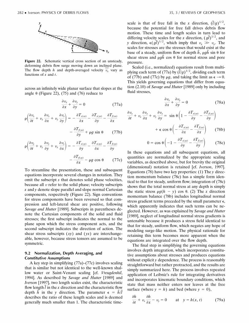
across an infinitely wide planar surface that slopes at theangle u (Figure 22), (75) and (76) reduce to

]vx

] x 1]vy

] y 5 0 (77a)

rS]vx

]t 1 vx

]vx

] x 1 vy

]vx

] y D 5 2]Ts~ xx!

] x 2]Ts~ yx!

] y 2]Tf~ xx!

] x

2]Tf~ yx!

] y 1 rg sin u (77b)

rS]vy

]t 1 vy

]vy

] y 1 vx

]vy

] x D 5 2]Ts~ yy!

] y 2]Ts~ xy!

] x 2]Tf~ yy!

] y

2]Tf~ xy!

] x 2 rg cos u (77c)

To streamline the presentation, these and subsequentequations incorporate several changes in notation. Theyomit the subscript s that denotes solid phase velocities,because all v refer to the solid phase; velocity subscriptsx and y denote slope parallel and slope normal Cartesiancomponents, respectively (Figure 22). Sign conventionsfor stress components have been reversed so that com-pression and left-lateral shear are positive, followingSavage and Hutter [1989]. Subscripts in parentheses de-note the Cartesian components of the solid and fluidstresses; the first subscript indicates the normal to theplane upon which the stress component acts, and thesecond subscript indicates the direction of action. Theshear stress subscripts ( xy) and ( yx) are interchange-able, however, because stress tensors are assumed to besymmetric.

9.2 Normalization, Depth Averaging, andConstitutive Assumptions

A key step in simplifying (77a)–(77c) involves scalingthat is similar but not identical to the well-known shal-low water or Saint-Venant scaling [cf. Vreugdenhil,1994]. As described by Savage and Hutter [1989] andIverson [1997], two length scales exist, the characteristicflow length l in the x direction and the characteristic flowdepth h in the y direction. The parameter e 5 h/ ldescribes the ratio of these length scales and is deemedgenerally much smaller than 1. The characteristic time-

scale is that of free fall in the x direction, ( l/g)1/ 2,because the potential for free fall drives debris flowmotion. These time and length scales in turn lead todiffering velocity scales for the x direction, ( g l)1/ 2, andy direction, e( g l)1/ 2, which imply that vx .. vy. Thescales for stresses are the stresses that would exist at thebase of a steady, uniform flow of depth h, rgh sin u forshear stress and rgh cos u for normal stress and porepressure.

Scaled (i.e., normalized) equations result from multi-plying each term of (77a) by ( l/g)1/ 2, dividing each termof (77b) and (77c) by rg, and taking the limit as e 3 0.This yields governing equations that differ from equa-tion (2.10) of Savage and Hutter [1989] only by includingfluid stresses,

]vx

] x 1]vy

] y 5 0 (78a)

]vx

]t 1 vx

]vx

] x 1 vy

]vx

] y 5 sin u S1 2]Ts~ yx!

] y 2]Tf~ yx!

] y D1 e cos u S2

]Ts~ xx!

] x 2]Tf~ xx!

] x D (78b)

0 5 cos u S21 2]Ts~ yy!

] y 2]Tf~ yy!

] y D (78c)

In these equations and all subsequent equations, allquantities are normalized by the appropriate scalingvariables, as described above, but for brevity the original(dimensional) notation is retained [cf. Iverson, 1997].Equations (78) have two key properties: (1) The y direc-tion momentum balance (78c) has a simple form iden-tical to that for steady, uniform flow; integration of (78c)shows that the total normal stress at any depth is simplythe static stress rg(h 2 y) cos u. (2) The x directionmomentum balance (78b) includes longitudinal normalstress gradient terms preceded by the small parameter e,which apparently indicates that such terms can be ne-glected. However, as was explained by Savage and Hutter[1989], neglect of longitudinal normal stress gradients isuntenable because it produces a stress field identical tothat for steady, uniform flow, which negates any hope ofmodeling surge-like motion. The physical rationale forretaining this term becomes more apparent when theequations are integrated over the flow depth.

The final step in simplifying the governing equationsinvolves depth integration, which incorporates constitu-tive assumptions about stresses and produces equationswithout explicit y dependence. The process is reasonablystraightforward but rather protracted, and the results aresimply summarized here. The process involves repeatedapplication of Leibniz’s rule for integrating derivativesand incorporates kinematic boundary conditions, whichstate that mass neither enters nor leaves at the freesurface (where y 5 h) and bed (where y 5 0),

]h]t 1 vx

]h] x 2 vy 5 0 at y 5 h~ x, t! (79a)

Figure 22. Schematic vertical cross section of an unsteady,deforming debris flow surge moving down an inclined plane.The flow depth h and depth-averaged velocity vx vary asfunctions of x and t.


vy 5 0 at y 5 0 (79b)

It also involves the assumption that the debris flowsurface is free of all stresses,

Ts~ xx! 5 Ts~ yy! 5 Ts~ yx! 5 Tf~ xx! 5 Tf~ yy! 5 Tf~ yx! 5 0 (80)

at y 5 h~ x, t!

and it employs depth-averaged velocities and normalstresses defined by

vx 51h E

0

h

vx d y (81a)

Ts~ xx! 51h E

0

h

Ts~ xx! d y (81b)

Ts~ yy! 51h E

0

h

Ts~ yy! d y (81c)

Tf~ xx! 51h E

0

h

Tf~ xx! d y (81d)

Tf~ yy! 51h E

0

h

Tf~ yy! d y (81e)

vx2 5

1h E

0

h

vx2 d y 5 jvx

2 (81f )

As was noted by Savage and Hutter [1989], values of j in(81f) that deviate from unity provide information aboutthe deviation of the vertical velocity profile from unifor-mity. If a debris flow moves exclusively by basal slip, j 51 applies. At the other extreme, j 5 6/5 applies for adebris flow with no basal sliding and a parabolic velocityprofile indicative of laminar viscous flow. As a result, theassumption j ' 1 appears generally justified.

More important than the details of the internal ve-locity field is the constitutive description of stresses in(78b). For the granular solids the stress model used hereis the simple Coulomb rule given by (6). The appropriatenondimensional form of the Coulomb rule is

Ts~ yx! 5 2sgn ~vx!Ts~ yy! cot u tan fbed/int (82)

in which fbed/int indicates the appropriate friction anglefor bed slip or internal deformation and sgn (vx) denotesthe sign (1 or 2) of vx. In (82), cot u appears because ofthe different scalings for shear and normal stress com-ponents. Although (82) does not contain pore pressureeffects explicitly, it does so implicitly because Ts( yy) andTf( yy) are related by (78c). Thus as fluid pressures Tf( yy)grow in magnitude, the magnitudes of Ts( yy) and Ts( yx)diminish.

The Coulomb rule also leads directly to an expression

relating Ts( xx) to Ts( yy), obtained from classical Rankine[1857] earth pressure theory. Earth pressure theory ap-plies to effective stresses borne by the solid constituents[Lambe and Whitman, 1979] and presumes a relation

Ts~ xx! 5 kact/passTs~ yy! (83)

in which kact/pass is an earth pressure coefficient that hasdifferent values depending on whether the flow is “ac-tively” extending (]vx/] x . 0) or “passively” compress-ing (]vx/] x , 0). For deformation that includes bothbed slip and internal slip, earth pressure theory leads tothe expression for kact/pass presented without derivationby Savage and Hutter [1989],

kact/pass 5 21 7 @1 2 cos2 fint~1 1 tan2 fbed!#

1/ 2

cos2 fint2 1

(84)

and derived in Appendix C. The “2” in “7” applies tothe active coefficient, and the “1” applies to the passive.Hungr [1995] suggested that the earth pressure relation(83) might be generalized by including the effects ofelastic compliance, but noted that the elastic modulushas negligible influence on model predictions.

Equations (78)–(84) provide all information neces-sary to complete the formulation of the hydraulic equa-tions. Integration of (78a) from y 5 0 to y 5 h, withapplication of the kinematic boundary conditions (79),produces a depth-averaged mass conservation equation,

]h]t 1

]~hvx!

] x 5 0 (85)

Integration of (78c) from y 5 0 to y 5 h yields a steadymomentum balance in the y direction, which states thatthe sum of the nondimensional solid and fluid stressbalances the y component of the nondimensional totalmixture weight

Ts~ yy! 1 Tf~ yy! 5 h~ x, t! 2 y (86)

This in turn leads to nondimensional expressions for thetotal (solid plus fluid) normal stress at the bed and forthe y direction depth-averaged total normal stress,

Ts~ yy! 1 Tf~ yy! 5 h at y 5 0 (87)

Ts~ yy! 1 Tf~ yy! 51h E

0

h

~h 2 y! d y 512 h (88)

Integration of the normalized x direction momentumequation (78b) from y 5 0 to y 5 h yields the result [cf.Savage and Hutter, 1989, equation (2.24)]


]

]t ~hvx! 1]

] x ~jhvx2! 5 h sin u

1 ~Ts~ yx!uy50! sin u 1 ~Tf~ yx!uy50! sin u

2 e cos u]

] x ~hTs~ xx!! 2 e cos u]

] x ~hTf~ xx!! (89)

Terms on the right-hand side of (89) can be inter-preted as follows. The first term represents the gravita-tional driving stress. The second term represents fric-tional resistance to slip at the base of the flow and can beevaluated by applying the Coulomb equation (82) andthe normal stress equation (87) at the flow base,

~Ts~ yx!uy50! sin u 5 2sgn ~vx!~h 2 pbed! cos u tan fbed

(90)

where h 2 pbed is the nondimensional basal effectivestress and pbed 5 Tf( yy)uy50 is the nondimensional basalpore pressure. The third term on the right-hand side of(89) represents flow resistance due to shear of the fluidat the flow base. It can be evaluated using Newton’s lawof viscosity (14), which yields

@~Tf~ yx!!uy50# sin u 5 2yfm~]vx/] y!uy50 (91)

where m is the appropriate, nondimensional depth-aver-aged viscosity, given by m 5 m/[rgh2/( gl#)1/ 2]. Applica-tion of (91) requires knowledge of the fluid velocitygradient at the bed, (]vx/] y)uy50, which is generallyunknown but can be obtained from estimates of thevertical velocity profile. The estimates are constrained byassuming no slip of fluid at the bed and a mean fluidvelocity of vx. For example, if the velocity profile islinear, then (]vx/] y)uy50 5 vx/h. If the velocity profile isparabolic, then a simple analysis of laminar flow down anincline shows that (]vx/] y)uy50 5 3vx/h [cf. Bird et al.,1960, pp. 37–40]. If the velocity profile is blunt, withshear strongly concentrated near the bed, a good de-scriptor is (]vx/] y)uy50 5 (n 1 2)(vx/h), where n 5 1indicates a parabolic profile and n . 1 indicates blunterprofiles; this form is used below. The fourth term on theright-hand side of (89) represents the longitudinal stressgradient due to interaction of solid grains. It can beevaluated using (83) and (88), yielding

2e cos u]

] x ~hTs~ xx!!

5 2ekact/pass cos u]

] x Sh2

2 2 hTf~ yy!D (92)

As is indicated by the presence of Tf( yy) in (92), thelongitudinal solid stress gradient is mediated by fluidpressure. The final term in (89) represents the longitu-dinal stress gradient due to the fluid pressure alone.Because fluid pressure is isotropic, it can be rewrittenwith Tf( yy)in place of Tf( xx),

2e cos u]

] x ~hTf~ xx!! 5 2e cos u]

] x ~hTf~ yy!! (93)

The utility of (92) and (93) is enhanced by evaluating theintegral (81e) to calculate Tf( yy) for a condition in whichthe fluid pressure increases linearly from zero at thedebris flow surface to a maximum of pbed at the bed (acondition consistent with the hydraulic theory assump-tions). The integration shows that ](hTf( yy))/] x 5h(]pbed/] x), and this substitution is used in (94) below.

9.3. Governing Equations and Auxiliary ConditionsThe final form of the x direction momentum equation

results from incorporating (85) and (90)–(93) in (89),assuming j 5 1, collecting and cancelling like terms, anddividing by h, which yields

]vx

]t 1 vx

]vx

] x 5 sin u 2 sgn ~vx!S1 2pbed

h D cos u tan fbed

2 yfm~n 1 2!Svx

h2D2 e cos u

]

] x @kact/pass~h 2 pbed! 1 pbed# (94)

Together, (94) and (85) form a set of two equations intwo unknowns, vx( x, t) and h( x, t), which can be solvedprovided that the basal pore fluid pressure pbed(x, t) andthe necessary initial and boundary conditions are speci-fied. The need to specify rather than predict basal porepressures is inherent to the hydraulic model; fluid pres-sure deviations from hydrostatic values result from ve-locity components normal to the bed (see section 8), andneglect of such velocities in (78c) precludes the possibil-ity of predicting nonhydrostatic pressures. Thus inclu-sion of nonhydrostatic pressures pbed( x, t) may seem tocontradict the hydraulic model assumptions. The inclu-sion is justified, however, on the grounds that the con-solidation process responsible for generating nonhydro-static fluid pressures (section 8) typically operates ontimescales substantially longer than the debris flow du-ration (Table 8). Thus as a first approximation, high porepressures, once established, may be assumed to persist indebris flows, and pore pressures may be treated as pa-rameters in hydraulic model calculations.

Inspection of the individual terms in (94) reveals howthe hydraulic model encapsulates debris flow physics.The inertial terms on the left-hand side of (94) show thatboth rigid body accelerations and convective accelera-tions may be important. On the right-hand side of (94),if the first two terms are viewed in isolation, they depicta static balance of forces identical to that used in infiniteslope stability analyses for cases in which there is zerocohesion and an arbitrary distribution of pore pressure[cf. Iverson, 1990, 1992]. If the last term on the right-hand side is included, this static force balance assumes aform comparable to that of two-dimensional slope sta-bility analyses that use methods of slices, and in this case


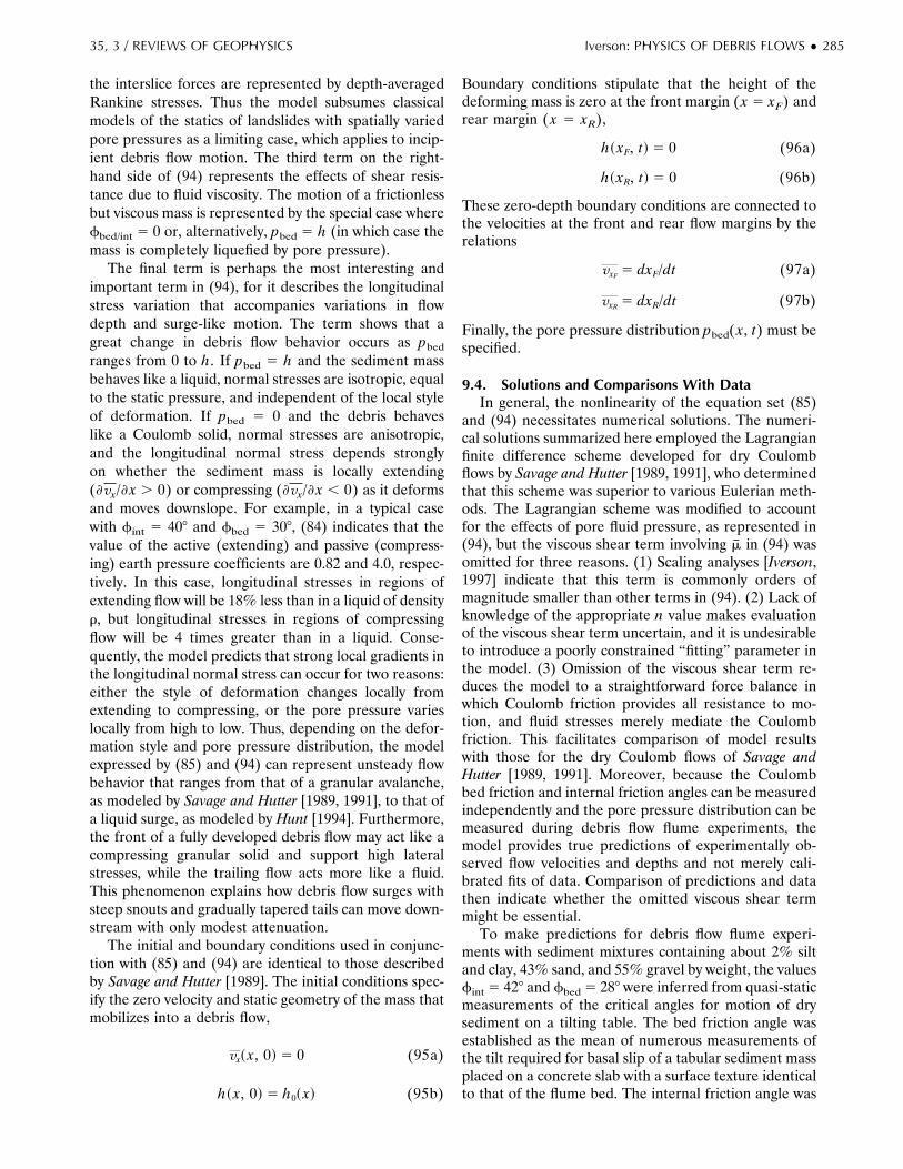
the interslice forces are represented by depth-averagedRankine stresses. Thus the model subsumes classicalmodels of the statics of landslides with spatially variedpore pressures as a limiting case, which applies to incip-ient debris flow motion. The third term on the right-hand side of (94) represents the effects of shear resis-tance due to fluid viscosity. The motion of a frictionlessbut viscous mass is represented by the special case wherefbed/int 5 0 or, alternatively, pbed 5 h (in which case themass is completely liquefied by pore pressure).

The final term is perhaps the most interesting andimportant term in (94), for it describes the longitudinalstress variation that accompanies variations in flowdepth and surge-like motion. The term shows that agreat change in debris flow behavior occurs as pbed

ranges from 0 to h. If pbed 5 h and the sediment massbehaves like a liquid, normal stresses are isotropic, equalto the static pressure, and independent of the local styleof deformation. If pbed 5 0 and the debris behaveslike a Coulomb solid, normal stresses are anisotropic,and the longitudinal normal stress depends stronglyon whether the sediment mass is locally extending(]vx/] x . 0) or compressing (]vx/] x , 0) as it deformsand moves downslope. For example, in a typical casewith fint 5 408 and fbed 5 308, (84) indicates that thevalue of the active (extending) and passive (compress-ing) earth pressure coefficients are 0.82 and 4.0, respec-tively. In this case, longitudinal stresses in regions ofextending flow will be 18% less than in a liquid of densityr, but longitudinal stresses in regions of compressingflow will be 4 times greater than in a liquid. Conse-quently, the model predicts that strong local gradients inthe longitudinal normal stress can occur for two reasons:either the style of deformation changes locally fromextending to compressing, or the pore pressure varieslocally from high to low. Thus, depending on the defor-mation style and pore pressure distribution, the modelexpressed by (85) and (94) can represent unsteady flowbehavior that ranges from that of a granular avalanche,as modeled by Savage and Hutter [1989, 1991], to that ofa liquid surge, as modeled by Hunt [1994]. Furthermore,the front of a fully developed debris flow may act like acompressing granular solid and support high lateralstresses, while the trailing flow acts more like a fluid.This phenomenon explains how debris flow surges withsteep snouts and gradually tapered tails can move down-stream with only modest attenuation.

The initial and boundary conditions used in conjunc-tion with (85) and (94) are identical to those describedby Savage and Hutter [1989]. The initial conditions spec-ify the zero velocity and static geometry of the mass thatmobilizes into a debris flow,

vx~ x, 0! 5 0 (95a)

h~ x, 0! 5 h0~ x! (95b)

Boundary conditions stipulate that the height of thedeforming mass is zero at the front margin ( x 5 xF) andrear margin ( x 5 xR),

h~ xF, t! 5 0 (96a)

h~ xR, t! 5 0 (96b)

These zero-depth boundary conditions are connected tothe velocities at the front and rear flow margins by therelations

vxF 5 dxF/dt (97a)

vxR 5 dxR/dt (97b)

Finally, the pore pressure distribution pbed( x, t) must bespecified.

9.4. Solutions and Comparisons With DataIn general, the nonlinearity of the equation set (85)

and (94) necessitates numerical solutions. The numeri-cal solutions summarized here employed the Lagrangianfinite difference scheme developed for dry Coulombflows by Savage and Hutter [1989, 1991], who determinedthat this scheme was superior to various Eulerian meth-ods. The Lagrangian scheme was modified to accountfor the effects of pore fluid pressure, as represented in(94), but the viscous shear term involving m in (94) wasomitted for three reasons. (1) Scaling analyses [Iverson,1997] indicate that this term is commonly orders ofmagnitude smaller than other terms in (94). (2) Lack ofknowledge of the appropriate n value makes evaluationof the viscous shear term uncertain, and it is undesirableto introduce a poorly constrained “fitting” parameter inthe model. (3) Omission of the viscous shear term re-duces the model to a straightforward force balance inwhich Coulomb friction provides all resistance to mo-tion, and fluid stresses merely mediate the Coulombfriction. This facilitates comparison of model resultswith those for the dry Coulomb flows of Savage andHutter [1989, 1991]. Moreover, because the Coulombbed friction and internal friction angles can be measuredindependently and the pore pressure distribution can bemeasured during debris flow flume experiments, themodel provides true predictions of experimentally ob-served flow velocities and depths and not merely cali-brated fits of data. Comparison of predictions and datathen indicate whether the omitted viscous shear termmight be essential.

To make predictions for debris flow flume experi-ments with sediment mixtures containing about 2% siltand clay, 43% sand, and 55% gravel by weight, the valuesfint 5 428 and fbed 5 288 were inferred from quasi-staticmeasurements of the critical angles for motion of drysediment on a tilting table. The bed friction angle wasestablished as the mean of numerous measurements ofthe tilt required for basal slip of a tabular sediment massplaced on a concrete slab with a surface texture identicalto that of the flume bed. The internal friction angle was


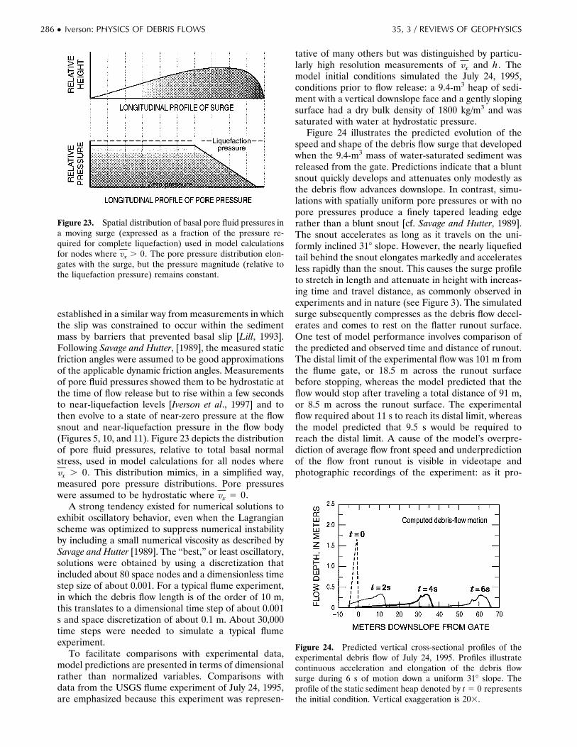
established in a similar way from measurements in whichthe slip was constrained to occur within the sedimentmass by barriers that prevented basal slip [Lill, 1993].Following Savage and Hutter, [1989], the measured staticfriction angles were assumed to be good approximationsof the applicable dynamic friction angles. Measurementsof pore fluid pressures showed them to be hydrostatic atthe time of flow release but to rise within a few secondsto near-liquefaction levels [Iverson et al., 1997] and tothen evolve to a state of near-zero pressure at the flowsnout and near-liquefaction pressure in the flow body(Figures 5, 10, and 11). Figure 23 depicts the distributionof pore fluid pressures, relative to total basal normalstress, used in model calculations for all nodes wherevx . 0. This distribution mimics, in a simplified way,measured pore pressure distributions. Pore pressureswere assumed to be hydrostatic where vx 5 0.

A strong tendency existed for numerical solutions toexhibit oscillatory behavior, even when the Lagrangianscheme was optimized to suppress numerical instabilityby including a small numerical viscosity as described bySavage and Hutter [1989]. The “best,” or least oscillatory,solutions were obtained by using a discretization thatincluded about 80 space nodes and a dimensionless timestep size of about 0.001. For a typical flume experiment,in which the debris flow length is of the order of 10 m,this translates to a dimensional time step of about 0.001s and space discretization of about 0.1 m. About 30,000time steps were needed to simulate a typical flumeexperiment.

To facilitate comparisons with experimental data,model predictions are presented in terms of dimensionalrather than normalized variables. Comparisons withdata from the USGS flume experiment of July 24, 1995,are emphasized because this experiment was represen-

tative of many others but was distinguished by particu-larly high resolution measurements of vx and h. Themodel initial conditions simulated the July 24, 1995,conditions prior to flow release: a 9.4-m3 heap of sedi-ment with a vertical downslope face and a gently slopingsurface had a dry bulk density of 1800 kg/m3 and wassaturated with water at hydrostatic pressure.

Figure 24 illustrates the predicted evolution of thespeed and shape of the debris flow surge that developedwhen the 9.4-m3 mass of water-saturated sediment wasreleased from the gate. Predictions indicate that a bluntsnout quickly develops and attenuates only modestly asthe debris flow advances downslope. In contrast, simu-lations with spatially uniform pore pressures or with nopore pressures produce a finely tapered leading edgerather than a blunt snout [cf. Savage and Hutter, 1989].The snout accelerates as long as it travels on the uni-formly inclined 318 slope. However, the nearly liquefiedtail behind the snout elongates markedly and acceleratesless rapidly than the snout. This causes the surge profileto stretch in length and attenuate in height with increas-ing time and travel distance, as commonly observed inexperiments and in nature (see Figure 3). The simulatedsurge subsequently compresses as the debris flow decel-erates and comes to rest on the flatter runout surface.One test of model performance involves comparison ofthe predicted and observed time and distance of runout.The distal limit of the experimental flow was 101 m fromthe flume gate, or 18.5 m across the runout surfacebefore stopping, whereas the model predicted that theflow would stop after traveling a total distance of 91 m,or 8.5 m across the runout surface. The experimentalflow required about 11 s to reach its distal limit, whereasthe model predicted that 9.5 s would be required toreach the distal limit. A cause of the model’s overpre-diction of average flow front speed and underpredictionof the flow front runout is visible in videotape andphotographic recordings of the experiment: as it pro-

Figure 23. Spatial distribution of basal pore fluid pressures ina moving surge (expressed as a fraction of the pressure re-quired for complete liquefaction) used in model calculationsfor nodes where vx . 0. The pore pressure distribution elon-gates with the surge, but the pressure magnitude (relative tothe liquefaction pressure) remains constant.

Figure 24. Predicted vertical cross-sectional profiles of theexperimental debris flow of July 24, 1995. Profiles illustratecontinuous acceleration and elongation of the debris flowsurge during 6 s of motion down a uniform 318 slope. Theprofile of the static sediment heap denoted by t 5 0 representsthe initial condition. Vertical exaggeration is 203.


gressed downslope, the flow segregated into three majorsurges plus several minor surges (Figure 25), whereasthe model simulates one coherent surge only. Segrega-tion into multiple surges appears to retard the averagespeed of the flow front but increase its ultimate runout.Depleted in size and momentum by loss of mass to thetrailing surges, the flow front decelerates quickly on therunout surface. Succeeding surges overtake the deceler-ating front and impart momentum that pushes the frontforward and delays its stoppage.

More quantitative tests of the model can be made bycomparing predicted and measured graphs of flow depthas a function of time at fixed measurement cross sec-tions. Figure 25 compares predictions with records offlow depth measured at three downstream cross sectionsduring the flume experiment of July 24, 1995. Measure-ments at a cross section 2 m downslope from the releasegate were made with an ultrasonic transceiver that pro-duced data with a time resolution of about 0.1 s anddepth resolution of about 0.05 m. Measurements at crosssections 33 m and 67 m downslope were made withhigh-precision laser triangulation systems that provideda time resolution of 0.001 s (the sampling frequency) anddepth resolution of 0.001 m. Comparison of the data andmodel predictions show that the model predicts thespeed of the advancing debris flow front very well andthe overall shape of the debris flow surge reasonablywell. However, it fails to predict some important details.The model underestimates the attenuation of the surgefront, it overestimates the attenuation of the waveformtail, and it does not simulate breakup of the surge intomultiple surges. The first two difficulties might be par-tially remedied by including the viscous shear term in themodel, and this is a logical next step. Accurate simula-tion of the instability that causes a single surge to de-volve into multiple surges is more difficult because itrequires unambiguous distinction between numericaland physical instabilities. This will likely require a newtype of analysis.

Overall, the success of the simple model that employs(85) and (94) as governing equations appears better thanexpected. The relatively rapid, thin debris flows in theUSGS flume are characterized by moderately large Sav-age numbers and Bagnold numbers (Table 5), so amodel that emphasizes Coulomb friction and excludesexplicit treatment of grain collisions might be expectedto perform poorly. However, collision-dominated flowsobey a relation between shear and normal stresses thatmimics the quasi-static Coulomb equation [Savage andHutter, 1991]. The ratio of shear to normal stresses,rather than their absolute magnitudes, determines thevalue of kact/pass in (94), and the term containing kact/passestablishes the surge-like character of the flow. There-fore although Coulomb stresses lack the shear rate de-pendence of collisional stresses, they can mimic theeffects of collisional stresses in some respects. A mo-mentum equation as simple as (94), with appropriateaccounting for viscous shear effects, might provide an

adequate model for predicting bulk motion of debrisflows. The model may be especially appropriate for lessenergetic debris flows in which shear rates are lower andgrain collisions figure less prominently than in the high-speed flows at the USGS flume.

10. CONCLUSION

Debris flows are gravity-driven surges of roughlyequal volumes of water and poorly sorted sediment,thoroughly mixed and agitated. Phenomena such as fine-sediment gravity currents or wet rock avalanches cansuperficially resemble debris flows but lack the strongsolid-fluid interactions that produce debris flows’ uniqueattributes. Interaction of solids and fluid gives debrisflows bulk mobilities (L/H) that commonly exceed thoseof comparably sized rock avalanches by 100%. Juxtapo-sition of solid and fluid forces allows debris flow mate-rials to slide or lock frictionally as well as to flow. Mostdebris flows commence as landslides triggered by in-creased pore water pressures, and most terminate asslowly consolidating sediment deposits. Between these

Figure 25. Comparison of measured and predicted flowdepths as a function of time for the experimental debris flow ofJuly 24, 1995. Predictions and data are shown for three crosssections, 2 m, 33 m, and 67 m downslope from the gate at theflume head. Flow commenced at the recorded time t 5 9.324s, and flow through all cross sections was on a uniform 318slope.


quasi-static stages of motion, debris flow behavior typi-cally is influenced by inertial forces and by a combina-tion of grain friction, grain collisions, and viscous fluidflow. Investigations of these influences indicate that tra-ditional Bingham and Bagnold models of debris behav-ior should be supplanted by models that account forinteractions of solid and fluid constituents.

Data from large-scale flume experiments provideclues to the character of momentum transfer in debrisflows. Measured stresses at the base of debris flowschange rapidly, and the relative magnitude of stressfluctuations increases as the area of the measurementsurface decreases. This indicates that individual grainsor groups of grains and adjacent fluid interact dynami-cally with the flow boundary, and probably with oneanother, and corroborates the visual impression thatdebris flows can violate no-slip boundary conditions anddevelop substantial grain fluctuation energy, or granulartemperature. Measured basal fluid pressures, whichchange asynchronously relative to the basal totalstresses, indicate that heads of debris flow surges gener-ally lack much fluid pressure, whereas the finer-grainedtails of surges are nearly liquefied by high fluid pressure.Interior fluid pressures remain elevated at near-lique-faction levels even during deposition, indicating thatdeposition results mainly from resistance at flow headsand margins.

Mixture theory provides an appropriate mathematicalframework for investigating debris flows. It indicatesthat fluid pressures greater than hydrostatic cannot per-sist during steady, uniform debris motion. Instead, highfluid pressures result from debris contraction (consoli-dation), which must be accompanied by local reductionof granular temperature and by globally unsteady mo-tion. This suggests that debris flow motion may be afundamentally unsteady phenomenon. As yet, however,no comprehensive model exists to calculate the coupled,simultaneous evolution of pore pressures and granulartemperatures in unsteady debris flows. Nonetheless, es-timates of characteristic timescales for dissipation ofexcess pore fluid pressures in debris flows show that theytypically exceed flow durations. Depth-averaged modelsof debris flow motion can therefore exploit the assump-tion that pore fluid pressures remain elevated for theduration of an event. A model of this type, derived bygeneralizing the Savage-Hutter model of dry flows ofCoulomb material, predicts the behavior of experimen-tal debris flows reasonably well.

Experimental debris flows, like many in nature, typi-cally have included no clasts with dimensions compara-ble to or greater than the flow depth and have beenconfined to channels with simple geometries. Modelsbased on classical continuum mechanics appear to workwell for describing such flows. However, natural debrisflows may encounter channels so tortuous or entrainboulders so large that continuum mechanical assump-tions fail. Discrete particle models, comparable to thedry avalanche model of Cleary and Campbell [1993],

might be required to understand debris flow behavior insuch circumstances. Furthermore, the apparent sensitiv-ity of debris flow motion to nuances in the positioning ofindividual boulders or flow path obstacles hints thatdebris flow motion may be mechanistically chaotic, atleast in some instances. Deterministic prediction ofsome aspects of debris flow behavior may thereforeprove impossible.

Future experimentation and modeling can probablyilluminate at least six key aspects of debris-flow physicswithout resolving the possibility of chaos or adopting themethodology of discrete-particle modeling:

1. Flow regimes in which grain friction, grain colli-sions, and fluid viscosity dominate can in principle bediscriminated on the basis of transition values of dimen-sionless parameters such as NBag, NSav, and NDar. Rig-orous experiments, in which one parameter is systemat-ically varied while others are held constant, should helpdefine the transition values. Once defined, these valuescan guide application of simplified models of debrisflows dominated by only one or two types of momentumtransfer.

2. Development of physically based understandingand modeling of mass gain and loss by moving debrisflows is essential for realistic predictions in many circum-stances. Incorporating mass change terms in mathemat-ical models is straightforward, but how to predict themagnitudes of mass change on the basis of boundary andflow properties remains unclear. Better understandingof erosion and sedimentation by debris flows will prob-ably require systematic experimentation.

3. Debris flows can move as a single surge, but theycommonly break into a series of surges of roughly similarmagnitude. Surge fronts carry the largest percentage oflarge clasts and commonly form the deepest part of theflow, and formation and segregation into multiple surgestherefore have great implications for hazards due toimpact and inundation. Although development of surgesfrom infinitesimal flow perturbations has been observedunder various field and experimental conditions, thephysics remain poorly understood. More experimentsand analyses are needed.

4. Pore-fluid pressures exert a strong influence ondebris flow mechanics. The influence can be modeledsimplistically by including realistic pore pressure distri-butions in appropriately formulated hydraulic models(e.g., section 9). However, a rigorous understanding ofpore pressure effects requires a fully coupled model inwhich pore pressures and granular temperatures evolvecontemporaneously from initiation through inertial mo-tion and subsequent deposition.

5. Grain size sorting that selectively moves the larg-est clasts to the surface and front of debris flow surgesmay play an essential role in controlling the pore pres-sure distribution. Sophisticated continuum models maybe able to account for sorting phenomena.

6. Models and experimental tests that provide un-derstanding of debris flows’ response to three-dimen-


sional topography are necessary for hazard forecasts inmany areas. Quasi-three-dimensional models that cap-ture some elements of debris flow behavior have beendeveloped recently by O’Brien et al. [1993], Lang and Leo[1994], and Hungr [1995], but further work to expandupon these models and include the effects of solid-fluidinteractions is desirable.

APPENDIX A: DERIVATION OF EQUATION (46)

Conservation of linear momentum by m2 during col-lision with m1 can be expressed with good approxima-tion by (46) if m1 .. m2. The approximation can bederived from exact equations for momentum conserva-tion during collision of two inelastic bodies traveling incolinear paths, which may be stated as [Spiegel, 1967, p.200–201]:

v0 5~m1 2 em2!~2v0! 1 m2~1 1 e!vup~tup!

m1 1 m2(A1)

v0down 5m1~1 1 e!~2v0! 1 ~m2 2 em1!vup~tup!

m1 1 m2(A2)

Here m1 has velocity v0 prior to the collision and 2v0after the collision; m2 has velocity vup(tup) prior to thecollision and v0down after the collision.

An effective coefficient of restitution e9 for behaviorof m2 during the collision may be defined exactly as

e9 5 2v0down

vup~tup!(A3)

An exact expression for e9 may be obtained by firstsolving (A1) for vup(tup), which yields

vup~tup! 5 v0S 2m1

m2~1 1 e!1

1 2 e1 1 eD (A4)

Substituting (A4) into (A2) then yields an expression forv0down that is linear in v0. Then substituting both thisexpression for v0down and (A4) into (A3) yields, aftersome manipulation,

e9 522 1 2e@2 1 ~m1/m2!#

2~m1/m2! 1 3 2 e 1 ~1 2 e!~m2/m1!(A5)

This equation is exact. Simplified versions of (A5) existfor the special case wherein m1 5 m2, which leads to theresult

e9 53e 2 13 2 e (A6)

and for the special case m1 .. m2, which gives the result

e9 < e (A7)

This approximation neglects all terms in (A5) that are ofthe order of 1 and smaller and retains terms of the orderof m1/m2.

Equation (46) is obtained from (A2) by using (A7)and replacing vup(tup) with the equivalent expression2v0down(1/e). The validity of the approximation can beinvestigated empirically by comparing values of e withthose of e9 calculated using (A5) (Table A1). The tab-ulated values indicate that the approximation error in-creases as values of m1/m2 and e decline. The error isless than 2%, however, if m1/m2 . 10 and e . 0.9, orif m1/m2 . 1000 and e . 0.1. The approximationappears useful as long as these or comparable conditionsare satisfied.

APPENDIX B: EXACT SOLUTIONS FOR BEHAVIOROF GRAIN m2

Exact, simultaneous solution of (44a)–(44d), (45),and (46) yields

tup 5 21B Sv0F 2e

1 1 e 1 ~e 2 1!m1

m2G 1

c

1 1 eD (B1)

tdown 5 21B Sv0F 2

1 1 e 2 ~e 2 1!m1

m2G 2

c

1 1 eD (B2)

v0down 5 2~m1/m2!ev0 (B3)

v0up 5 ev0S 21 1 e 1

m1

m2D 1

c

1 1 e (B4)

s 5 21

2B FS2v0 2 c

1 1 e 1 v0

m1

m2D2

2 e2v02Sm1

m2D2G (B5)

c 5 v0~1 2 e!S2m2

m1

1 1 e1 1 e2 1 2 1

m1

m2~1 1 e!D

z S2m2

m1

1 1 e1 1 e2 1 1D21

(B6)

The equation for c, (B6), is critical because c appears inmost of the other equations and has great physicalsignificance. If e 5 1, then c 5 0, which implies thatgrain fluctuation energy lost to bed friction exactly bal-ances the production of fluctuation energy by working ofthe bed shear stress. If e , 1, as is true for inelasticsediment grains, then c . 0, which implies that produc-tion of fluctuation energy must more than compensate

TABLE A1. Values of e* Calculated From (A5) for VariousValues of e and m1/m2

Value ofm1/m2

Value of e9

e 5 0.1 e 5 0.5 e 5 0.9 e 5 1.0

10 0.017 0.443 0.886 1.0100 0.091 0.494 0.899 1.0

1000 0.099 0.499 0.900 1.0

Comparison of the tabulated e9 values with the associated e valuesshows the error of the approximation e 5 e9.


for bed friction in order to sustain the oscillating motionof grain m2.

APPENDIX C: DERIVATION OF EQUATION (84)

The earth pressure coefficient equation (84) can bederived with reference to the Mohr stress circle andCoulomb failure envelopes depicted in Figure C1 [cf.Savage and Hutter, 1989]. The diagram illustrates thestate of stress in a Coulomb mass that is simultaneouslysliding along the bed, where the friction angle is fbed,and failing internally, where the friction angle is fint.The basic equations necessary to obtain the expressionfor kact/pass are

Ts~ yx! 5 Ts~ yy! tan fbed (C1)

tmax 5 Ts~mean! sin fint (C2)

Ts~mean! 1 b 5 Ts~ yy! (C3)

b2 1 Ts~ yx!2 5 tmax

2 (C4)

kact/pass 5Ts~ xx!

Ts~ yy!5 21 1 2

Ts~mean!

Ts~ yy!(C5)

Equations (C1) and (C2) state the Coulomb failure rulefor bed slip and internal slip, respectively. Equations(C3) and (C4) state simple geometric relations evidentin Figure C1. Like (C1) and (C2), (C3) and (C4) applyfor both the active (extensional) and passive (compres-sional) failure states. Equation (C5) provides a usefulalternative definition of kact/pass in terms of the mean

normal stress, Ts(mean) 5 12 (Ts( xx) 1 Ts( yy)). This

quantity, like the quantities b and tmax, is defined graph-ically in Figure C6. Physically, tmax is the maximum shearstress attainable in the failing mass, and b is the differ-ence between the y direction normal stress Ts( yy) and themean normal stress.

The initial steps in the derivation consist of substitut-ing (C4) into (C2), substituting (C1) into the resultingequation, and then substituting (C3) into this equation.This produces the result

@Ts~ yy! 2 Ts~mean!#2 5 Ts~mean!

2 sin2 fint 2 Ts~ yy!2 tan2 fbed

(C6)Regrouping terms in this equation, using the identity1 2 sin2 fint 5 cos2 fint, and dividing all terms byTs( yy)

2 (1 1 tan2 fbed) then yields

cos2 fint

1 1 tan2 fbedSTs~mean!

Ts~ yy!D2

22

1 1 tan2 fbedSTs~mean!

Ts~ yy!D

1 1 5 0 (C7)

This is a quadratic equation in Ts(mean)/Ts(yy), which may besolved by the standard quadratic formula, yielding

Ts~mean!

Ts~ yy!5

1 7 @1 2 cos2 fint~1 1 tan2 fbed!#1/ 2

cos2 fint(C8)

which is obtained after some algebraic simplification.Substitution of (C8) into (C5) then yields (84). Note thatthis derivation and Figure C1 assume fbed , fint; oth-erwise, fbed is irrelevant because all deformation occursinternally. In the event that fbed . fint, the term involv-

Figure C1. Mohr stress circle and Coulomb failure envelopes for a granular material that is simultaneouslyslipping along a bed and failing internally. The radius of the stress circle defines the maximum internal shearstress, tmax.


ing fbed in (C8) and (84) can be ignored, and (84)reduces to the standard form of the Rankine equationfor deforming granular media without basal sliding [e.g.,Lamb and Whitman, 1979, p. 164].

NOTATION

a factor characterizing dependence ofpermeability on porosity.

A viscous relaxation rate, equal to yfm/ysrsk, 1/T.b difference between y direction and mean

normal stress, M/LT2.B buoyancy-adjusted gravity, equal to

(1 2 rf/rs) gy, L/T2.c cohesive strength, M/LT2.

C mixture compressibility, LT2/M.C1 constant of integration, L/T.C2 constant of integration, L.

d total derivative operator.D material derivative operator (following

motion of solids).Dh hydraulic diffusivity, L2/T.

e coefficient of restitution of solid grains.E composite mixture stiffness, equal to 1/C,

M/LT2.f solid-fluid interaction force per unit volume

of mixture, M/L2T2.F magnitude of instantaneous grain impulse

force, ML/T2.Favg time-averaged value of F, ML/T2.

g gravitational acceleration, L/T2.g magnitude of g, L/T2.

gy y component of g, L/T2.h debris flow thickness normal to bed, L.h characteristic value of h, L.H vertical distance of debris flow descent from

source area, L.i subscript denoting inertial component of

stress.I identity tensor.j conductive flux of granular temperature per

unit volume, M/T3.k hydraulic permeability, L2.

kact/pass Rankine earth pressure coefficient.K hydraulic conductivity, L/T.l length of head of debris flow surge, L.l characteristic length (parallel to bed) of

debris flow surge, L.L horizontal distance of debris flow runout

from source area, L.ms mass influx rate of solids per unit debris

flow volume, M/TL3.mf mass influx rate of fluid per unit debris flow

volume, M/TL3.m1 mass of grains overlying basal shear zone, M.m2 mass of grain within basal shear layer, M.M total mass of debris flow, M.

n viscous power law coefficient.N number of grains above slip surface.

NBag Bagnold number.NDar Darcy number.Nfric friction number.

Nmass mass number.NRey grain Reynolds number.NSav Savage number.

p pore fluid pressure, M/LT2.pbed normalized pore fluid pressure at bed.pdev deviation of p from hydrostatic value, M/LT2.

q subscript denoting quasi-static component ofstress.

q Darcian specific discharge of pore fluid, L/T.R bulk flow resistance coefficient.s mean free path of grain motion, L.t time, T.

tD time duration of debris flow from initiationto deposition, T.

tdiff timescale for pore pressure diffusion, T.tup time of upward motion of grain m2 between

successive contacts, T.tdown time of downward motion of grain m2

between successive contacts, T.tcycle tup 1 tdown, T.

Ts solid phase stress tensor, M/LT2.Tf fluid phase stress tensor, M/LT2.

Ts2f solid-fluid interaction stress tensor, M/LT2.Te effective stress tensor, M/LT2.T9 extra stress tensor in solid-fluid mixture

modeled as single phase, M/LT2.T depth-averaged stress component, M/LT2.u displacement of solid grain from initial

position, L.v velocity magnitude, L/T.v mixture velocity, L/T.

vs solid phase velocity, L/T.vf fluid phase velocity, L/T.vs time-averaged mean value of vs, L/T.v9s fluctuation of vs about its mean value, L/T.vy component of vs normal to bed, L/T.vx component of vs parallel to bed, L/T.vx depth-averaged value of vx, L/T.

vset grain settling velocity, L/T.v0 initial velocity of grain m1 following contact

with m2, L/T.vup upward-bound velocity of grain m2, L/T.

vdown downward-bound velocity of grain m2, L/T.v0up initial value of vup following grain contact

with bed, L/T.v0down initial value of vdown following grain contact

with overlying mass, L/T.w debris flow width, L.x coordinate directed parallel to bed, L.

x9 x coordinate that translates downslope withvelocity vx, L.

y coordinate directed normal to bed, L.z vertical coordinate, L.


a mass percentage of fines in sediment mixture.g shear strain rate, 1/T.G rate of degradation of granular temperature

to heat per unit volume, M/LT3.d characteristic grain diameter, L.e debris flow aspect ratio, equal to h/ l.u slope angle.k sediment-water mixture compression

coefficient.l Bagnold’s [1954] linear concentration of solids.m dynamic viscosity of pore fluid with

suspended fine sediment, M/LT.mw dynamic viscosity of pure water, M/LT.

j momentum distribution coefficient fordepth-averaged flow.

r mass density of debris flow mixture, M/L3.ra added-mass density of solids accelerating

through fluid, M/L3.rb mass density of body of debris flow surge,

M/L3.rf mass density of debris flow fluid

constituents, M/L3.rh mass density of head of debris flow surge, M/L3.rs mass density of debris flow solid

constituents, M/L3.rw mass density of pure water, M/L3.

rdry dry (dehydrated) bulk density of debris flowmixture, M/L3.

s total normal compressive stress, M/LT2.S stress (generic), M/LT2.t shear stress, M/LT2.

tmax maximum shear stress, M/LT2.T granular temperature, L2/T2.yf volume fraction of pore fluid, (equal to

porosity in saturated mixture).ys volume fraction of granular solids

(ys 1 yf 5 1 in saturated mixture).yfines volume fraction of fine grains (silt plus clay).

f bulk friction angle.fg grain friction angle.

fbed friction angle for sliding along bed.fint friction angle for internal deformation.

c fluctuation velocity generated by graininteraction with bed, L/T.

= gradient operator, 1/L.=z divergence operator, 1/L.] partial derivative operator.

^ functional operator (generic).0 subscript denoting reference state.: scalar product of tensors and dyads [cf. Bird

et al., 1960].

ACKNOWLEDGMENTS. Rick LaHusen was instrumen-tal in devising and implementing electronic data collectionsystems at the USGS debris flow flume. Jon Major collectedand consolidated the data on debris flow deposits formedduring flume experiments. Dave McTigue, Jon Major, Joe

Walder, Mark Reid, Jim Vallance, Bill Savage, Ron Shreve,Stephen Grand, Neal Iverson, and Sue Knight provided usefulcritiques of the manuscript.

James A. Smith was the editor responsible for this paper.He thanks Dave McTigue, William Savage, and Ronald Shrevefor their technical reviews and Steven Grand for serving as across-disciplinary referee.

REFERENCES

Abbott, J., L. A. Mondy, A. L. Graham, and H. Brenner,Techniques for analyzing the behavior of concentrated sus-pensions, in Particulate Two-Phase Flow, edited by M. C.Roco, pp. 3–32, Butterworth-Heinemann, Newton, Mass.,1993.

Acrivos, A., The rheology of concentrated suspensions of non-colloidal particles, in Particulate Two-Phase Flow, edited byM. C. Roco, pp. 169–189, Butterworth-Heinemann, New-ton, Mass., 1993.

Adams, M. J., and B. J. Briscoe, Deterministic micromechani-cal modeling of failure or flow in discrete planes of denselypacked particle assemblies: Introductory principles, inGranular Matter, edited by A. Mehta, pp. 259–291, Spring-er-Verlag, New York, 1994.

Anderson, K. G., and R. Jackson, A comparison of someproposed equations of motion of granular materials forfully developed flow down inclined planes, J. Fluid Mech.,241, 145–168, 1992.

Anderson, S. A., and N. Sitar, Analysis of rainfall-induceddebris flows, J. Geotech. Eng., 121, 544–552, 1995.

Arattano, M., and W. Z. Savage, Modelling debris flows askinematic waves, Bull. Int. Assoc. Eng. Geol., 49, 3–13, 1994.

Atkin, R. J., and R. E. Craine, Continuum theories of mixtures:Basic theory and historical development, Q. J. Mech. Appl.Math., Part 2, 29, 209–244, 1976.

Bagnold, R. A., Experiments on a gravity-free dispersion oflarge solid spheres in a Newtonian fluid under shear, Proc.R. Soc. London, Ser. A, 225, 49–63, 1954.

Batchelor, G. K., and J. T. Green, The determination of thebulk stress in a suspension of spherical particles to order c2,J. Fluid Mech., 56, 401–427, 1972.

Bear, J., Dynamics of Fluids in Porous Media, 764 pp., Dover,Mineola, N. Y., 1972.

Been, K., and G. C. Sills, Self-weight consolidation of soft soils:An experimental and theoretical study, Geotechnique, 31,519–535, 1981.

Beverage, J. P., and J. K. Culbertson, Hyperconcentrations ofsuspended sediment, J. Hydraul. Div. Am. Soc. Civ. Eng.,90(HY6), 117–128, 1964.

Biot, M. A., General theory of three-dimensional consolida-tion, J. Appl. Phys., 12, 155–164, 1941.

Bird, R. B., W. E. Stewart, and E. N. Lightfoot, TransportPhenomena, 780 pp., John Wiley, New York, 1960.

Bird, R. B., G. C. Dai, and B. J. Yaruso, The rheology and flowof viscoplastic materials, Rev. Chem. Eng., 1, 1–70, 1982.

Bishop, A. W., The stability of tips and spoil heaps, Q. J. Eng.Geol., 6, 335–376, 1973.

Blake, G. R., Bulk density, in Methods of Soil Analysis, editedby C. A. Black et al., pp. 374–390, Am. Soc. of Agron.,Madison, Wis., 1965.

Bridgman, P. W., Dimensional Analysis, Yale Univ. Press, NewHaven, Conn., 1922.

Bridgwater, J., M. H. Cooke, and A. M. Scott, Inter-particlepercolation: Equipment development and mean percola-tion velocities, Trans. Inst. Chem. Eng., 56, 157–167, 1978.

Bromhead, E. N., The Stability of Slopes, 374 pp., Chapman andHall, New York, 1986.


Buckingham, E., Model experiments and the form of empiricalequations, Trans. ASME, 37, 263, 1915.

Campbell, C. S., Rapid granular flows, Annu. Rev. Fluid Mech.,22, 57–92, 1990.

Cannon, S. H., and W. Z. Savage, A mass-change model for theestimation of debris-flow runout, J. Geol., 96, 221–227, 1988.

Caruso, P., and M. T. Pareschi, Estimation of lahar and lahar-runout flow hydrograph on natural beds, Environ. Geol., 22,141–152, 1993.

Casagrande, A., Liquefaction and cyclic deformation ofsands—A critical review, Harvard Soil Mech. Ser., 88, 51 pp.,1976.

Chandler, R. N., and D. L. Johnson, The equivalence ofquasi-static flow in fluid-saturated porous media and Biot’sslow wave in the limit of zero frequency, J. Appl. Phys., 52,3391–3395, 1981.

Chapman, S., and T. G. Cowling, Mathematical Theory ofNonuniform Gases, 3rd ed., 423 pp., Cambridge Univ. Press,New York, 1970.

Chen, C., Comprehensive review of debris flow modeling con-cepts in Japan, in Debris Flows/Avalanches: Process, Recog-nition, and Mitigation, Rev. Eng. Geol., vol. 7, edited by J. E.Costa and G. F. Wieczorek, pp. 13–29, Geol. Soc. of Am.,Boulder, Colo., 1987.

Chen, C., Generalized viscoplastic modeling of debris flow, J.Hydraul. Eng., 114, 237–258, 1988a.

Chen, C., General solutions for viscoplastic debris flow, J.Hydraul. Eng., 114, 259–282, 1988b.

Cleary, P. W., and C. S. Campbell, Self-lubrication by longrunout landslides: Examination by computer simulation, J.Geophys. Res., 98(B12), 21,911–21,924, 1993.

Coleman, P. F., A new explanation for debris flow surgephenomena (abstract), Eos Trans. AGU, 74(16), SpringMeet. Suppl., 154, 1993.

Costa, J. E., Physical geomorphology of debris flows, in Devel-opments and Applications of Geomorphology, edited by J. E.Costa and P. J. Fleisher, pp. 268–317, Springer-Verlag,New York, 1984.

Costa, J. E., and G. F. Wieczorek (Eds.), Debris Flows/Ava-lanches: Process, Recognition, and Mitigation, Rev. Eng.Geol., vol. 7, 239 pp., Geol. Soc. of Am., Boulder, Colo.,1987.

Costa, J. E., and G. P. Williams, Debris-flow dynamics (video-tape), U.S. Geol. Surv. Open File Rep., 84-606, 22 min., 1984.

Coussot, P., Structural similarity and transition from Newto-nian to non-Newtonian behavior for clay-water suspensions,Phys. Rev. Lett., 74, 3971–3974, 1995.

Coussot, P., and J.-M. Piau, On the behavior of fine mudsuspensions, Rheol. Acta, 33, 175–184, 1994.

Coussot, P., and J.-M. Piau, The effects of an addition offorce-free particles on the rheological properties of finesuspensions, Can. Geotech. J., 32, 263–270, 1995.

Coussot, P., and S. Proust, Slow unconfined spreading of amudflow, J. Geophys. Res., 101(B11), 25,217–25,229, 1996.

Daido, A., On the occurrence of mud-debris flow, Bull. DisasterPrev. Res. Inst. Kyoto Univ., Part 2, 21(187), 109–135, 1971.

Davies, T. R. H., Spreading of rock avalanche debris by me-chanical fluidization, Rock Mech., 15, 9–24, 1982.

Davies, T. R. H., Large debris flows: A macroviscous phenom-enon, Acta Mech., 63, 161–178, 1986.

Davies, T. R. H., Debris-flow surges—A laboratory investiga-tion, Mitt. 96, 122 pp., Versuchsanst. fur Wasserbau, Hy-drologie und Glaziologie, Zurich, Switzerland, 1988.

Davies, T. R. H., Debris-flow surges—Experimental simula-tion, N. Z. J. Hydrol., 29, 18–46, 1990.

DiFelice, R., The voidage function for fluid-particle interac-tion systems, Int. J. Multiphase Flow, 20, 153–159, 1994.

Drake, T. G., Structural features in granular flows, J. Geophys.Res., 95(B6), 8681–8696, 1990.

Eckersley, D., Instrumented laboratory flowslides, Geotech-nique, 40, 489–502, 1990.

Einstein, A., A new determination of molecular dimensions (inGerman), Ann. Phys., 19, 289–306, 1906. (English transla-tion by A. D. Cowper in Investigations on the Theory ofBrownian Movement, edited by R. Furth, pp. 38–62, Dover,Mineola, N. Y., 1956.)

Ellen, S. D., and R. W. Fleming, Mobilization of debris flowsfrom soil slips, San Francisco Bay region, California, inDebris Flows/Avalanches: Process, Recognition, and Mitiga-tion, Rev. Eng. Geol., vol. 7, edited by J. E. Costa and G. F.Wieczorek, pp. 31–40, Geol. Soc. of Am., Boulder, Colo.,1987.

Erlichson, H., A mass-change model for the estimation ofdebris-flow runout, A second discussion: Conditions for theapplication of the rocket equation, J. Geol., 99, 633–634,1991.

Fairchild, L. H., and M. Wigmosta, Dynamic and volumetriccharacteristics of the 18 May 1980 lahars on the ToutleRiver, Washington, in Proceedings of the Symposium onErosion Control in Volcanic Areas Tech. Mem. 1908, pp.131–153, Jpn. Public Works Res. Inst., Min. of Constr.,Tokyo, 1983.

Fink, J. H., M. C. Malin, R. E. D’Alli, and R. Greeley,Rheological properties of mudflows associated with thespring 1980 eruptions of Mount St. Helens volcano, Wash-ington, Geophys. Res. Lett., 8, 43–46, 1981.

Frankel, N. A., and A. Acrivos, On the viscosity of a concen-trated suspension of solid spheres, Chem. Eng. Sci., 22,847–853, 1967.

Garcia-Aragon, J. A., Granular-fluid chute flow: Experimentaland numerical observations, J. Hydraul. Eng., 121, 355–364,1995.

Gibson, R. E., G. L. England, and M. J. L. Hussey, The theoryof one-dimensional consolidation of saturated clays, 1, Fi-nite nonlinear consolidation of thin homogeneous layers,Geotechnique, 17, 261–273, 1967.

Haff, P. K., Grain flow as a fluid-mechanical phenomenon, J.Fluid Mech., 134, 401–430, 1983.

Haff, P. K., A physical picture of kinetic granular fluids,J. Rheol., 30, 931–948, 1986.

Hampton, M. A., Buoyancy in debris flows, J. Sediment. Petrol.,49, 753–758, 1979.

Hampton, M. A., H. J. Lee, and J. Locat, Submarine land-slides, Rev. Geophys., 34, 33–59, 1996.

Hanes, D. M., and D. L. Inman, Experimental evaluation of adynamic yield criterion for granular fluid flows, J. Geophys.Res., 90(B5), 3670–3674, 1985.

Hayashi, J. N., and S. Self, A comparison of pyroclastic flowand debris avalanche mobility, J. Geophys. Res., 97(B6),9063–9071, 1992.

Heim, A., Bergsturz und Menschenleben, 218 pp., Fretz undWasmuth, Zurich, Switzerland, 1932.

Helm, D. C., Conceptual aspects of subsidence due to fluidwithdrawal, in Recent Trends in Hydrogeology, edited by T.N. Narasimhan, Spec. Pap. Geol. Soc. Am., 189, 103–139,1982.

Henderson, F. M., Open Channel Flow, 522 pp., Macmillan,New York, 1966.

Hill, H. M., Bed forms due to a fluid stream, J. Hydraul. Div.Am. Soc. Civ. Eng., 92, 127–143, 1966.

Hooke, R. L., Mass movement in semi-arid environments andthe morphology of alluvial fans, in Slope Stability—Geotech-nical Engineering and Geomorphology, edited by M. G.Anderson and K. S. Richards, pp. 505–529, John Wiley,New York, 1987.

Hopkins, M. A., J. T. Jenkins, and M. Y. Louge, On thestructure of three-dimensional shear flows, Mech. Mater.,16, 179–187, 1993.


Howard, T. R., J. E. Baldwin II, and H. F. Donley, Landslidesin Pacifica, California, caused by the storm, in Landslides,Floods and Marine Effects of the Storm of January 3–5, 1982,in the San Francisco Bay Region, California, edited by S. D.Ellen and G. F. Wieczorek, U.S. Geol. Surv. Prof. Pap.,1434, 163–184, 1988.

Hsu, K. J., Catastrophic debris streams (sturzstroms) gener-ated by rockfalls, Geol. Soc. Am. Bull., 86, 129–140, 1975.

Hui, K., and P. K. Haff, Kinetic grain flow in a vertical channel,Int. J. Multiphase Flow., 12, 289–298, 1986.

Hungr, O., A mass-change model for the estimation of debris-flow runout: A discussion, J. Geol., 98, 791, 1990.

Hungr, O., A model for the runout analysis of rapid flow slides,debris flows, and avalanches, Can. Geotech. J., 32, 610–623,1995.

Hungr, O., and N. R. Morgenstern, High velocity ring sheartests on sand, Geotechnique, 34, 415–421, 1984.

Hunt, B., Newtonian fluid mechanics treatment of debris flowsand avalanches, J. Hydraul. Eng., 120, 1350–1363, 1994.

Hutchinson, J. N., A sliding-consolidation model for flowslides, Can. Geotech. J., 23, 115–126, 1986.

Hutter, K., B. Svendsen, and D. Rickenmann, Debris-flowmodeling: A review, Continuum Mech. Thermodyn., 8, 1–35,1996.

Innes, J. L., Debris flows, Prog. Phys. Geogr., 7, 469–501, 1983.Iverson, R. M., A constitutive equation for mass-movement

behavior, J. Geol., 93, 143–160, 1985.Iverson, R. M., Unsteady, nonuniform landslide motion, 1,

Theoretical dynamics and the steady datum state, J. Geol.,94, 1–15, 1986a.

Iverson, R. M., Unsteady, nonuniform landslide motion, 2,Linearized theory and the kinematics of transient response,J. Geol., 94, 349–364, 1986b.

Iverson, R. M., Groundwater flow fields in infinite slopes,Geotechnique, 40, 139–143, 1990.

Iverson, R. M., Sensitivity of stability analyses to groundwaterdata, in Landslides (Proceedings of the Sixth InternationalSymposium on Landslides, 1), edited by D. H. Bell, pp.451–457, A. A. Balkema, Rotterdam, Netherlands, 1992.

Iverson, R. M., Differential equations governing slip-inducedpore-pressure fluctuations in a water-saturated granularmedium, Math. Geol., 23, 1027–1048, 1993.

Iverson, R. M., Hydraulic modeling of unsteady debris-flowsurges with solid-fluid interactions, in Proceedings of theFirst International Conference on Debris-Flow Hazards Miti-gation, Am. Soc. of Civ. Eng., New York, in press, 1997.

Iverson, R. M., and R. P. Denlinger, The physics of debrisflows—A conceptual assessment, in Erosion and Sedimen-tation in the Pacific Rim, edited by R. L. Beschta et al., IAHSPubl., 165, 155–165, 1987.

Iverson, R. M., and R. G. LaHusen, Dynamic pore-pressurefluctuations in rapidly shearing granular materials, Science,246, 769–799, 1989.

Iverson, R. M., and R. G. LaHusen, Friction in debris flows:Inferences from large-scale flume experiments, HydraulicEngineering ’93 (Proceedings of the 1993 Conference of theHydraulics Division of the American Society of Civil Engi-neers), vol. 2, 1604–1609, Am. Soc. of Civ. Eng., New York,1993.

Iverson, R. M., and J. J. Major, Groundwater seepage vectorsand the potential for hillslope failure and debris flow mo-bilization, Water Resour. Res., 22, 1543–1548, 1986.

Iverson, R. M., and M. E. Reid, Gravity-driven groundwaterflow and slope failure potential, 1, Elastic effective-stressmodel, Water Resour. Res., 28, 925–938, 1992.

Iverson, R. M., J. E. Costa, and R. G. LaHusen, Debris-flowflume at H. J. Andrews Experimental Forest, Oregon, U.S.Geol. Surv. Open File Rep., 92-483, 2 pp., 1992.

Iverson, R. M., M. E. Reid, and R. G. LaHusen, Debris-flow

mobilization from landslides, Ann. Rev. Earth Planet. Sci.,25, 85–138, 1997.

Jaeger, H. M., and S. R. Nagel, Physics of the granular state,Science, 255, 1523–1531, 1992.

Jahns, R. H., Desert floods, Contrib. 499, pp. 10–15, Calif. Inst.of Technol., Pasadena, 1949.

Jenkins, J. T., Rapid granular flow down inclines, Appl. Mech.Rev., Part 2, 47(6), S240–S244, 1994.

Jenkins, J. T., and E. Askari, Hydraulic theory for a debris flowsupported by a collisional shear layer, Proceedings of theInternational Association for Hydraulic Research Interna-tional Workshop on Floods and Inundations Related to LargeEarth Movements, Trent, Italy, 1994, A6.1–A6.10, Int. Assoc.for Hydraul. Res., Delft, Netherlands, 1994.

Jenkins, J. T., and D. F. McTigue, Transport processes inconcentrated suspensions: The role of particle fluctuations,in Two Phase Flows and Waves, edited by D. D. Joseph andD. G. Schaeffer, pp. 70–79, Springer-Verlag, New York,1990.

Jenkins, J. T., and S. B. Savage, A theory for the rapid flow ofidentical, smooth, nearly elastic particles, J. Fluid Mech.,130, 187–202, 1983.

Johnson, A. M., A model for debris flow, Ph.D. dissertation,Pa. State Univ., State College, 1965.

Johnson, A. M., Physical Processes in Geology, 557 pp., W. H.Freeman, New York, 1970.

Johnson, A. M., Debris flow, in Slope Instability, edited byD. Brunsden and D. B. Prior, pp. 257–361, John Wiley, NewYork, 1984.

Johnson, G., M. Massoudi, and K. R. Rajagopal, A review ofinteraction mechanisms in fluid-solid flows, Tech. Rep.DOE/PETC/TR-90/9, U.S. Dep. of Energy, 54 pp., Pitts-burgh Energy Technol. Cent., Pittsburgh, Pa., 1990.

Johnson, G., M. Massoudi, and K. R. Rajagopal, Flow of asolid-fluid mixture between flat plates, Chem. Eng. Sci., 46,1713–1723, 1991.

Khegai, A. Y., N. V. Popov, P. A. Plekhanov, and V. A.Keremkulov, Experiments at the Chemolgan debris-flowtesting ground, Kazakhstan, Landslide News, 6, 27–28, Jpn.Landslide Soc., Kyoto, 1992.

Kytomaa, H. K., and C. M. Atkinson, Sound propagation insuspensions and acoustic imaging of their microstructure,Mech. Mater., 16, 189–197, 1993.

Lambe, T. W., and R. V. Whitman, Soil Mechanics, SI Version,553 pp., John Wiley, New York, 1979.

Lang, R. M., and B. R. Leo, Model for avalanches in threespatial dimensions, CRREL Rep. 94-5, 23 pp., U.S. ArmyCorps of Eng. Cold Reg. Res. and Eng. Lab., Hanover,N. H., 1994.

Lee, J., S. C. Cowin, and J. S. Templeton III, An experimentalstudy of the kinematics of flow through hoppers, Trans. Soc.Rheol., 18, 247–269, 1974.

Li, J., and J. Yuan, The main features of the mudflows inJiang-Jia Ravine, Z. Geomorphol., 27, 326–341, 1983.

Li, T., A model for predicting the extent of a major rockfall, Z.Geomorphol., 27, 473–482, 1983.

Li, V. C., Estimation of in-situ hydraulic diffusivity of rockmasses, Pure Appl. Geophys., 122, 545–559, 1985.

Lighthill, M. J., and G. B. Whitham, On kinematic waves, 1,Flood movement in long rivers, Proc. R. Soc. London, Ser.A, 229, 281–316, 1955.

Lill, T., A critical evaluation of a new method for determiningthe angle of internal friction for cohesionless sediments,B.S. thesis, 37 pp., Beloit Coll., Beloit, Wis., 1993.

Lun, C. K., S. B. Savage, D. J. Jeffrey, and N. Chepurny,Kinetic theories for granular flow: Inelastic particles inCouette flow and slightly inelastic particles in a general flowfield, J. Fluid Mech., 140, 223–256, 1984.

Macedonio, G., and M. T. Pareschi, Numerical simulation of


some lahars from Mount St. Helens, J. Volcanol. Geotherm.Res., 54, 65–80, 1992.

Major, J. J., Experimental studies of deposition by debris flows:Process, characteristics of deposits and effects of pore-fluidpressure, 341 pp., Ph.D. dissertation, Univ. of Wash., Seat-tle, 1996.

Major, J. J., Depositional processes in large-scale debris-flowexperiments, J. Geol., 105, 345–366, 1997.

Major, J. J., and T. C. Pierson, Debris flow rheology: Experi-mental analysis of fine-grained slurries, Water Resour. Res.,28, 841–857, 1992.

Major, J. J., and B. Voight, Sedimentology and clast orienta-tions of the 18 May 1980 southwest-flank lahars, Mount St.Helens, Washington, J. Sediment. Petrol., 56, 691–705, 1986.

Malekzadeh, M. J., Flow of liquid-solid mixtures down inclinedchutes, Ph.D. thesis, 212 pp., McGill Univ., Montreal, Que.,Canada, 1993.

McTigue, D. F., and J. T. Jenkins, Channel flow of a concen-trated suspension, in Advances in Micromechanics of Gran-ular Materials, edited by H. H. Shen, pp. 381–390, Elsevier,New York, 1992.

Middleton, G., Experimental studies related to the problem offlysch sedimentation, Geol. Assoc. Can. Spec. Pap., 7, 253–272, 1970.

Mitchell, J. K., Fundamentals of Soil Behavior, 422 pp., JohnWiley, New York, 1976.

Miyamoto, K., and S. Egashira, Mud and debris flows, J.Hydrosci. Hydraul. Eng. Jpn. Soc. Civ. Eng., SI-2, 1–19, 1993.

Mohrig, D., G. Parker, and K. X. Whipple, Hydroplaning ofsubaqueous debris flows (abstract), Eos Trans. AGU,76(46), Fall Meet. Suppl., F277, 1995.

Morton, D. M., and R. H. Campbell, Spring mudflows atWrightwood, southern California, Q. J. Eng. Geol., 7, 377–384, 1974.

O’Brien, J. S., and P. Y. Julien, Laboratory analysis of mudflowproperties, J. Hydraul. Eng., 114, 877–887, 1988.

O’Brien, J. S., P. Y. Julien, and W. T. Fullerton, Two-dimen-sional water flood and mudflow simulation, J. Hydraul. Eng.,119, 244–261, 1993.

Ogata, A., Theory of dispersion in a granular medium, U.S.Geol. Surv. Prof. Pap., 411-I, 34 pp., 1970.

Ogawa, S., Multitemperature theory of granular materials, inProceedings of the U.S.-Japan Seminar on Continuum-Me-chanics and Statistical Approaches to the Mechanics of Gran-ular Materials, pp. 208–217, Gukujutsu Bunken Fukyukai,Tokyo, 1978.

Ohsumi Works Office, Debris Flow at Sakurajima, 2, 81 pp.,Jpn. Min. of Constr., Kagoshima, 1995.

Okuda, S., H. Suwa, K. Okunishi, K. Yokoyama, andM. Nakano, Observations on the motion of a debris flowand its geomorphological effects, Z. Geomorphol., suppl. 35,142–163, 1980.

Onada, G. Y., and E. G. Liniger, Random loose packings andthe dilatancy onset, Phys. Rev. Lett., 64, 2727–2730, 1990.

Passman, S. L., and D. F. McTigue, A new approach to theeffective stress principle, in Compressibility Phenomena inSubsidence, edited by S. K. Saxena, pp. 79–91, Eng. Found.,New York, 1986.

Phillips, C. J., and T. R. H. Davies, Determining rheologicalproperties of debris flow material, Geomorphology, 4, 101–110, 1991.

Pierson, T. C., Erosion and deposition by debris flows at Mt.Thomas, North Canterbury, New Zealand, Earth Surf. Pro-cesses, 5, 227–247, 1980.

Pierson, T. C., Dominant particle support mechanisms in de-bris flows at Mt. Thomas, New Zealand, and implicationsfor flow mobility, Sedimentology, 28, 49–60, 1981.

Pierson, T. C., Initiation and flow behavior of the 1980 Pine

Creek and Muddy river lahars, Mount St. Helens, Wash-ington, Geol. Soc. Am. Bull., 96, 1056–1069, 1985.

Pierson, T. C., Flow behavior of channelized debris flows,Mount St. Helens, Washington, in Hillslope Processes, ed-ited by A. D. Abrahams, pp. 269–296, Allen and Unwin,Winchester, Mass., 1986.

Pierson, T. C., Flow characteristics of large eruption-triggereddebris flows at snow-clad volcanoes: Constraints for debris-flow models, J. Volcanol. Geotherm. Res., 66, 283–294, 1995.

Pierson, T. C., and J. E. Costa, A rheologic classification ofsubaerial sediment-water flows, in Debris Flows/Avalanches:Process, Recognition, and Mitigation, Rev. Eng. Geol., vol. 7,edited by J. E. Costa and G. F. Wieczorek, pp. 1–12, Geol.Soc. of Am., Boulder, Colo., 1987.

Pierson, T. C., and K. M. Scott, Downstream dilution of alahar: Transition from debris flow to hyperconcentratedstreamflow, Water Resour. Res., 21, 1511–1524, 1985.

Pierson, T. C., R. J. Janda, J. C. Thouret, and C. A. Borrero,Perturbation and melting of snow and ice by the 13 Novem-ber 1985 eruption of Nevado del Ruiz, Colombia, andconsequent mobilization, flow, and deposition of lahars, J.Volcanol. Geotherm. Res., 41, 17–66, 1990.

Plafker, G., and G. E. Ericksen, Nevado Huascaran ava-lanches, Peru, in Rockslides and Avalanches, vol. 1, NaturalPhenomena, edited by B. Voight, pp. 277–314, Elsevier,New York, 1978.

Poletto, M., and D. D. Joseph, Effective density and viscosityof a suspension, J. Rheol., 39, 323–343, 1995.

Prior, D. B., and J. M. Coleman, Submarine Slope Instability,in Slope Instability, edited by D. Brunsden and D. B. Prior,pp. 419–455, John Wiley, New York, 1984.

Rankine, W. J. M., On the stability of loose earth, Philos.Trans. R. Soc. London, 1857.

Reid, M. E., and R. M. Iverson, Gravity-driven groundwaterflow and slope failure potential, 2, Effects of slope mor-phology, material properties, and hydraulic heterogeneity,Water Resour. Res., 22, 939–950, 1992.

Rice, J. R., and M. P. Cleary, Some basic stress diffusionsolutions for fluid-saturated elastic porous media with com-pressible constituents, Rev. Geophys., 14, 227–241, 1976.

Rodine, J. D., and A. M. Johnson, The ability of debris heavilyfreighted with coarse clastic materials to flow on gentleslopes, Sedimentology, 23, 213–224, 1976.

Roeloffs, E., Poroelastic techniques in the study of earth-quake-induced hydrologic phenomena, Adv. Geophys., 37,133–195, 1996.

Rogers, C. D. F., T. A. Dijkstra, and I. J. Smalley, Particlepacking from an Earth science viewpoint, Earth ScienceReviews, 36, 59–92, 1994.

Rosato, A., K. J. Strandburg, F. Prinz, and R. H. Swendsen,Why the Brazil nuts are on top: Size segregation of partic-ulate matter by shaking, Phys. Rev. Lett., 25, 1038–1040, 1987.

Sabo Publicity Center, Debris flow at Sakurajima Volcano,videotape with audio in English, Ohsumi Work Off., KyushuReg. Constr. Bur., Jpn. Min. of Constr., Kagoshima, 1988.

Sassa, K., The mechanism starting liquefied landslides anddebris flows, in Proceedings of the Fourth International Sym-posium on Landslides, vol. 2, pp. 349–354, Int. Soc. for SoilMech. and Found. Eng., Toronto, Ont., Canada, 1984.

Sassa, K., The mechanism of debris flow, in Proceedings of theEleventh International Conference on Soil Mechanics andFoundation Engineering, pp. 1173–1176, A. A. Balkema,Rotterdam, Netherlands, 1985.

Savage, S. B., The mechanics of rapid granular flows, Adv.Appl. Mech., 24, 289–366, 1984.

Savage, S. B., Interparticle percolation and segregation ingranular materials: A review, in Developments in Engineer-ing Mechanics, edited by A. P. S. Selvadurai, pp. 347–363,Elsevier, New York, 1987.


Savage, S. B., Mechanics of debris flows, in Hydraulic Engineer-ing ’93 (Proceedings of the 1993 Conference of the HydraulicsDivision of the American Society of Civil Engineers), vol. 2,1402–1407, Am. Soc. of Civ. Eng., New York, 1993.

Savage, S. B., and K. Hutter, The motion of a finite mass ofgranular material down a rough incline, J. Fluid Mech., 199,177–215, 1989.

Savage, S. B., and K. Hutter, The dynamics of avalanches ofgranular materials from initiation to runout, I, Analysis,Acta Mech., 86, 201–223, 1991.

Savage, S. B., and S. McKeown, Shear stresses developedduring rapid shear of dense concentrations of large spher-ical particles between concentric cylinders, J. Fluid Mech.,127, 453–472, 1983.

Savage, S. B., and M. Sayed, Stresses developed in dry cohe-sionless granular materials sheared in an annular shear cell,J. Fluid Mech., 142, 391–430, 1984.

Savage, W. Z., and W. K. Smith, A model for the plastic flowof landslides, U.S. Geological Survey Prof. Pap., 1385, 32 pp.,1986.

Scheidegger, A. E., On the prediction of the reach and velocityof catastrophic landslides, Rock Mech., 5, 231–236, 1973.

Scott, K. M., J. W. Vallance, and P. T. Pringle, Sedimentology,behavior, and hazards of debris flows at Mount Rainier,Washington, U.S. Geol. Surv. Prof. Pap., 1547, 56 pp., 1995.

Sharp, R. P., and L. H. Nobles, Mudflow of 1941 at Wright-wood, southern California, Geol. Soc. Am. Bull., 64, 547–560, 1953.

Shen, H., and N. L. Ackerman, Constitutive relationships forsolid-fluid mixtures, J. Eng. Mech. Div. Am. Soc. Civ. Eng.,108, 748–763, 1982.

Shibata, M., and C. C. Mei, Slow parallel flows of a water-granule mixture under gravity, I, Continuum modeling,Acta Mech., 63, 179–193, 1986a.

Shibata, M., and C. C. Mei, Slow parallel flows of a water-granule mixture under gravity, II, Examples of free surfaceand channel flows, Acta Mech., 63, 195–216, 1986b.

Shieh, C.-L., Jan, C.-D., and Y.-F. Tsai, A numerical simula-tion of debris flow and its application, Nat. Hazards, 13,39–54, 1996.

Shlemon, R. J., R. H. Wright, and D. R. Montgomery, Anat-omy of a debris flow, Pacifica, California, in Debris Flows/Avalanches: Process, Recognition, and Mitigation, Rev. Eng.Geol., vol. 7, edited by J. E. Costa and G. F. Wieczorek, pp.181–200, Geol. Soc. of Am., Boulder, Colo., 1987.

Siebert, L., Large volcanic debris avalanches; Characteristics ofsource areas, deposits, and associated eruptions, J. Volca-nol. Geotherm. Res., 22, 163–197, 1984.

Sitar, N., S. A. Anderson, and K. A. Johnson, Conditions forinitiation of rainfall-induced debris flows, in Stability andPerformance of Slopes and Embankments II Proceedings, pp.834–849 Geotech. Eng. Div., Am. Soc. of Civ. Eng., NewYork, 1992.

Skempton, A. W., Long-term stability of clay slopes, Geotech-nique, 14, 75–101, 1964.

Skempton, A. W., Residual strength of clays in landslides,folded strata and the laboratory, Geotechnique, 35, 3–18, 1985.

Spiegel, M. R., Theoretical Mechanics, Schaum’s Outline Series,368 pp., McGraw-Hill, New York, 1967.

Suwa, H., Focusing mechanism of large boulders to a debris-flow front, Trans. Jpn. Geomorphol. Union, 9, 151–178, 1988.

Takahashi, T., Mechanical characteristics of debris flow, J.Hydraul. Div. Am. Soc. Civ. Eng., 104, 1153–1169, 1978.

Takahashi, T., Debris flow on prismatic open channel, J. Hy-draul. Div. Am. Soc. Civ. Eng., 106, 381–396, 1980.

Takahashi, T., Debris flow, Annu. Rev. Fluid Mech., 13, 57–77,1981.

Takahashi, T., Debris Flow, 165 pp., A. A. Balkema, Brook-field, Vt., 1991.

Takahashi, T. (Ed.), Japan-China joint research on the pre-vention from debris flow hazards, Res. Rep. 03044085, 195pp., Grant-in-Aid for Scientific Research, Jpn. Min. ofEduc. Sci. and Cult. Int. Sci. Res. Program, Tokyo, 1994.

Terzaghi, K., Stress conditions for the failure of concrete androck, Proc. Am. Soc. Test. Mater., 45, 777–801, 1945.

Thomas, D. G., Transport characteristics of suspension, VII, Anote on the viscosity of Newtonian suspensions of uniformspherical particles, J. Colloid Sci., 20, 267–277, 1965.

U.S. Geological Survey (USGS), Debris flow hazards in theSan Francisco Bay region, U.S. Geol. Surv. Fact Sheet,112-95, 4 pp., 1995.

Vaid, Y. P., and J. Thomas, Liquefaction and postliquefactionbehavior of sand, J. Geotech. Eng., 121, 163–173, 1995.

Vallance, J. W., Experimental and field studies related to thebehavior of granular mass flows and the characteristics oftheir deposits, Ph.D. dissertation, 197 pp., Mich. Technol.Univ., Houghton, 1994.

Vallance, J. W., and K. M. Scott, The Osceola mudflow fromMount Rainier: Sedimentology and hazard implications ofa huge clay-rich debris flow, Geol. Soc. Am. Bull., 109(2),143–163, 1997.

Vanoni, V. A. (Ed.), Sedimentation Engineering, 745 pp., Am.Soc. of Civ. Eng., New York, 1975.

Varnes, D. J., Slope movement types and processes, in Land-slides—Analysis and Control, edited by R. L. Schuster andR. J. Krizek, Spec. Rep. Natl. Res. Counc. Transp. Res.Board, 176, pp. 11–33, Natl. Acad. of Sci., Washington,D. C., 1978.

Vignaux, M., and G. J. Weir, A general model for Mt. Rua-pehu lahars, Bull. Volcanol., 52, 381–390, 1990.

Vreugdenhil, C. B., Numerical Methods for Shallow-WaterFlow, 261 pp., Kluwer Acad., Norwell, Mass., 1994.

Walton, O., Numerical simulation of inelastic, frictional parti-cle-particle interactions, in Particulate Two-Phase Flow, ed-ited by M. C. Roco, pp. 884–911, Butterworth-Heinemann,Newton, Mass., 1993.

Weir, G. J., Kinematic wave theory for Ruapehu lahars, N. Z.J. Sci., 25, 197–203, 1982.

Whipple, K. X., Debris-flow fans: Process and form, Ph.D.dissertation, 205 pp., Univ. of Washington, Seattle, 1994.

Whipple, K. X., and T. Dunne, The influence of debris-flowrheology on fan morphology, Owens Valley, California,Geol. Soc. Am. Bull., 104, 887–900, 1992.

Wieczorek, G. F., E. L. Harp, R. K. Mark, and A. K. Bhatta-charyya, Debris flows and other landslides in San Mateo,Santa Cruz, Contra Costa, Alameda, Napa, Solano,Sonoma, Lake, and Yolo counties, and factors influencingdebris-flow distribution, in Landslides, Floods and MarineEffects of the Storm of January 3–5, 1982, in the San Fran-cisco Bay Region, California, edited by S. D. Ellen and G. F.Wieczorek, U.S. Geol. Surv. Prof. Pap., 1434, 133–162, 1988.

Wierich, F. H., The generation of turbidity currents by sub-aerial debris flows, Geol. Soc. Am. Bull., 101, 278–291, 1989.

Yamashita, S., and K. Miyamoto, Numerical simulationmethod of debris movements with a volcanic eruption,paper presented at Japan-U.S. Workshop on Snow Ava-lanche, Landslide and Debris Flow Prediction and Control,Jpn. Sci. and Technol. Agency, Tsukuba, 1991.

Yano, K., and A. Daido, Fundamental study on mud-flow, Bull.Disaster Prev. Res. Inst. Kyoto Univ., 14, 69–83, 1965.

Zhang, Y., and C. S. Campbell, The interface between fluid-like and solid-like behaviour in two-dimensional granularflows, J. Fluid Mech., 237, 541–568, 1992.

R. M. Iverson, Cascades Volcano Observatory, U.S. Geo-logical Survey, 5400 MacArthur Boulevard, Vancouver, WA98661. (e-mail: [email protected])


the physics of debris flows - william bechtel's...

Documents