valley incision by debris flows: evidence of a topographic signature

Valley incision by debris flows: Evidence of a topographic

signature

J. Stock and W. E. Dietrich

Department of Earth and Planetary Science, University of California, Berkeley, California, USA

Received 9 November 2001; accepted 9 October 2002; published 9 April 2003.

[1] The sculpture of valleys by flowing water is widely recognized, and simplifiedmodels of incision by this process (e.g., the stream power law) are the basis for mostrecent landscape evolution models. Under steady state conditions a stream power lawpredicts that channel slope varies as an inverse power law of drainage area. Using bothcontour maps and laser altimetry, we find that this inverse power law rarely extends toslopes greater than �0.03 to 0.10, values below which debris flows rarely travel.Instead, with decreasing drainage area the rate of increase in slope declines, leading to acurved relationship on a log-log plot of slope against drainage area. Fieldwork in thewestern United States and Taiwan indicates that debris flow incision of bedrockvalley floors tends to terminate upstream of where strath terraces begin and where area-slope data follow fluvial power laws. These observations lead us to propose that thesteeper portions of unglaciated valley networks of landscapes steep enough to producemass failures are predominately cut by debris flows, whose topographic signature is anarea-slope plot that curves in log-log space. This matters greatly as valleys with curvedarea-slope plots are both extensive by length (>80% of large steepland basins) andcomprise large fractions of main stem valley relief (25–100%). As a consequence,valleys carved by debris flows, not rivers, bound most hillslopes in unglaciatedsteeplands. Debris flow scour of these valleys appears to limit the height of some mountainsto substantially lower elevations than river incision laws would predict, an effect absent incurrent landscape evolution models. We anticipate that an understanding of debris flowincision, for which we currently lack even an empirical expression, would substantiallychange model results and inferences drawn about linkages between landscape morphologyand tectonics, climate, and geology. INDEX TERMS: 1824 Hydrology: Geomorphology (1625);

1815 Hydrology: Erosion and sedimentation; 3250 Mathematical Geophysics: Fractals and multifractals;

KEYWORDS: debris flows, erosion, incision, landscape evolution, stream power

Citation: Stock, J., and W. E. Dietrich, Valley incision by debris flows: Evidence of a topographic signature, Water Resour. Res.,

39(4), 1089, doi:10.1029/2001WR001057, 2003.

1. Introduction

[2] The sculpture of Earth’s unglaciated valleys by waterhas long been explored to understand both the processesand rates that create and maintain valleys [e.g., Playfair,1802; Gilbert, 1877; Davis, 1902; Horton, 1945]. Theseearly workers recognized that strath terraces borderingrivers and the adjustment of tributaries to main stems areevidence that rivers incise valleys. These visible signs oflowering, and the fascination with river longitudinal profileshape led to early speculation by nineteenth century work-ers [e.g., Gilbert, 1877] that rivers cut through Earth’scrust at rates determined by water discharge and channelslope (S) for a given substrate (K). The recognition thatvalley incision may transmit the effects of climate changeand tectonism throughout the landscape has led to arenewed interest in the problem of bedrock river incisionand its erosion laws. The first and simplest approach was

to assume that fluvial processes cut most unglaciatedvalleys, and that lowering rate was either a function ofboundary shear stress or stream power (w). For instance,Howard and Kerby [1983] proposed that bedrock incisionrate @z/@t was a power function of shear stress applied tothe bed by a moving fluid so that:

�@z=@t ¼ K1tb ¼ K1 rwgRSð Þb ð1Þ

where z is elevation (positive upward), K1 is a measure ofbed erodibility, t is shear stress, b is unknown, rw is fluiddensity, R is hydraulic radius and S is slope. In the spirit ofBagnold [1966], Seidl and Dietrich [1992] proposed thatbedrock lowering rate was proportional to work/unit timedone on the river bed (i.e., power) so that

�@z=@t ¼ wn ¼ rwgQSð Þn ð2Þ

where n is an unknown exponent and Q is discharge. Asreviewed by many others [e.g., Sklar and Dietrich, 1998;Whipple and Tucker, 1999], expressions (1) and (2) can be

Copyright 2003 by the American Geophysical Union.0043-1397/03/2001WR001057$09.00

ESG 1 - 1

WATER RESOURCES RESEARCH, VOL. 39, NO. 4, 1089, doi:10.1029/2001WR001057, 2003

parameterized in terms of drainage area and slope usinghydraulic relations, so that they take the form

@z=@t ¼ U� KAm Sn ð3Þ

where U is rock uplift rate, S is slope, and m and n areexponents whose values are debated but may be calibratedby direct measurement of erosion rates [e.g., Howard andKerby, 1983; Seidl et al., 1994; Whipple et al., 2000] orlongitudinal profile fitting [e.g., Seidl and Dietrich, 1992;Rosenbloom and Anderson, 1994; Stock and Montgomery,1999; Snyder et al., 2000; Kirby and Whipple, 2001]. Whenrock uplift rate and lowering rate are balanced so that thevalley long-profile is at steady state, the expression leads tothe expectation that

S ¼ U=K½ �1=n A�m=n ð4aÞ

or

log S ¼ log U=Kð Þ1=n�m=n log A ð4bÞ

[3] Availability of topography as DEMs (digital elevationmodels) and the desire to invert landforms quantitatively forerosion rate invites much use of equation (3). The expres-sion has been used to infer parameters in the stream powerlaw from area-slope data (see above) and the response ofriver profiles to tectonism [Snyder et al., 2000; Lague et al.,2000; Kirby and Whipple, 2001] or climate change [Tuckerand Slingerland, 1997; Whipple et al., 1999]. Most recentlandscape evolution models use some form of equation (3)to model valley incision, either by including the possibilityof alluvial channels which require the calculation of thedivergence of sediment transport [e.g., Willgoose et al.,1991; Howard, 1994; Tucker and Slingerland, 1994; Kooiand Beaumont, 1996; Howard, 1997; Tucker and Bras,1998; van der Beek and Braun, 1999] or by assuming thatbedrock river incision is the dominant process shapingchannel long-profiles [e.g., Anderson, 1994; Whipple andTucker, 1999; Whipple et al., 1999; Davy and Crave, 2000;Willett et al., 2001]. This long (yet incomplete) reference listis a measure of the reliance placed upon area-slope for-mulations like equation (3) to answer questions of wide-spread interest, like the response of landforms to climatechange or rock uplift.[4] Yet, little attention is paid to the extent of the valley

network in which the stream power law is valid. Forinstance, in the steeplands of the western United Stateswe have not observed field evidence for long-term bedrockriver incision (like a strath terrace) above valley slopes of0.05–0.10, a region below which debris flows rarely travel,and where well-developed fluvial bed forms like step-poolsoccur [e.g., Montgomery and Buffington, 1997]. Nor is itobvious that the power law trend observed in area-slopeplots of many rivers [e.g., Flint, 1974] can be projectedupstream of the steepest reaches where strath terraces arecommonly observed (e.g., Figure 1b). Upstream lies a steepvalley network whose properties are largely unexplored,where other processes such as debris flows are capable ofcarving valleys (e.g., Figure 2). Here topography is con-vergent in planform, but valleys lack banks or other fluvialfeatures that define channels (e.g., Figure 3). Hillslopes

deposit coarse, unsorted material in these valleys, leadingsome to call them colluvial valleys [Montgomery andBuffington, 1997]. The coarsest sediment size is oftenmeters in dimension, many times the common water flowdepth. In steeplands capable of generating landslides, thebulk of down valley sediment transport is by debris flows[e.g., Dietrich and Dunne, 1978; Benda, 1990]. Case studiesin the Oregon Coast Range and other steeplands documentthat debris flows are rarely mobile below valley slopes of0.02–0.05 (Table 1) although confinement, grain-size, fluidpressure, volume and junction angle also play a role [e.g.,Hungr et al., 1984; Benda and Cundy, 1990; Iverson, 1997].The apparent lower limit of 0.02–0.05 in Table 1 corre-sponds to slopes reported for step-pool bed forms ofMontgomery and Buffington [1997], while higher terminalslope values above 0.10 are typical of open slopes or fans inglaciated areas like British Columbia, Switzerland andScandinavia. These observations lead to the expectationthat valley network incision above slopes of 0.02–0.05 isinfluenced (at least in part) by debris flows.[5] Perhaps because of the poor resolution of most

DEMs, these valleys are often written about as if they were

Figure 1. (a) Hypothetical topographic signatures forhillslope and valley processes. Area and slope are measuredincrementally up valley main stem to the valley head. (b)Area-slope data from hand measurement of 1:24,000topographic map and field observations of strath terraces,Deer Creek, Santa Cruz Mountains. Rightmost two datapoints are from 1:100,000 scale maps of San Lorenzo River.The data in Figure 1b appear to require more than oneerosion law because a power law fit has nonrandomresiduals.

ESG 1 - 2 STOCK AND DIETRICH: VALLEY INCISION BY DEBRIS FLOWS

part of hillslopes. For instance, some have found a changein power law slope (or a scaling break) in area-slope datafrom DEMs such that valley slope ceases to change belowa certain drainage area. This has been inferred to representa transition to hillslope processes (Figure 1a) [e.g., Ijjasz-Vasquez and Bras, 1995; Moglen and Bras, 1995; Lagueet al., 2000]. But this scaling break is inferred to occur at0.1–1 km2, drainage areas at which valleys may occur. Bycontrast, others interpret the appearance of a scaling breakas the topographic signature for debris flow valley incision[Seidl and Dietrich, 1992; Montgomery and Foufoula-Geourgiu, 1993; Sklar and Dietrich, 1998]. With theexception of Howard [1998], there are no proposals fora debris flow incision law or rule. When we started ourinvestigations, little field evidence had been used to testeither hypothesis. Examples of each are shown graphicallyin Figure 1a, from which two focused questions arise:what is the location of the scaling break (if any) and whatis the form of the area-slope data above it? Since the formof area-slope data in steeplands could indicate a nonfluvialincision law, the location of the scaling break could definethe extent of fluvial incision in steeplands. Given thewidespread use of some form of stream power law,answers to these two questions have substantial implica-tions for both landscape evolution models and geomorphictheory.[6] In this paper we investigate the notion that debris flow

valley incision in unglaciated steeplands has an area-slope

topographic signature distinct from that of bedrock riverincision (Figure 1b). To do so, we avoid collection of datafrom hillslopes, and focus exclusively on valleys, whichreflect concentrative erosional processes. We report resultsfrom visits to sites of recent debris flows where we observedevidence for bedrock lowering along their run out. Usingboth high- and low-resolution topography, we examinearea-slope plots to see if they have a common form alongthe debris flow run out path. We also measure main stemarea and slope for larger, unglaciated steepland valleyswhere the form of area-slope data follow fluvial power lawsat large drainage areas, but may have a different form in thevalley headwaters where we have mapped older debris flowdeposits. We ask if the down valley disappearance of debrisflow deposits and appearance of strath terraces (wherepresent) has a consistent signature, such as a scaling break,that might separate fluvial from debris flow valley incision.Finally, we plot main stem valley slope and area fromUnited States 1:24,000 and global 1:50,000 maps to inves-tigate the generality of such signatures, and by inference thegenerality of debris flow valley incision in unglaciatedmountain ranges.

2. Site Selection

[7] To investigate if debris flows imprint a topographicsignature on valley longitudinal profiles, we visited sites ofrecent (<1 year-old) and historically recorded debris flows

Figure 2. Debris flow valley network in an Oregon Coast Range clear-cut. The combination of elevatedwater pressure during a 1996 storm and reduced root strength initiated landslides at valley heads thatmobilized as debris flows, scouring sediment and Tyee sandstone (white areas) along the runout. Road attop right indicates scale.

STOCK AND DIETRICH: VALLEY INCISION BY DEBRIS FLOWS ESG 1 - 3

in the western United States (Table 2). Although these siteswere selected opportunistically, they span a wide range ofclimates and erosion rates from soil-mantled sandstoneterrain lowering at 0.1 mm/yr (Oregon Coast Range), tosemi-arid, bedrock-dominated gneissic terrain eroding at �1mm/yr (San Bernardino Mountains). In these valleys (num-bers 1–16 in Table 2) we measured area and slope from

laser altimetry (Sullivan, Scottsburg and Roseburg) or1:24,000 USGS topography, and walked the run out ofdebris flows looking for evidence of bedrock erosion. InTable 2 we report deposition slopes measured in the fieldover the last 10 m of run out, or from high-resolutiontopography. These slopes tend to be higher than values from1:24,000 maps for the same reach. Deposition slopes for

Figure 3. View of bedrock valley bottom of Sullivan 1 (see Figure 5) in the Oregon Coast Rangeseveral months after scour by a debris flow. Note the surface parallel fractures in the Tyee Formation,some of which have been removed by the debris flow in the valley axis. In nearby untorrented valleys,unsorted hillslope deposits cover the bedrock.


historic debris flows in the Wasatch Range are from fanslopes on 1:24,000 maps.[8] With the goal of distinguishing river-cut valleys from

those cut by debris flows, we selected river basins fromsteeplands with a range of rock uplift rate and climateincluding the San Gabriel Mountains, California CoastRange, King Range, Oregon Coast Range and Taiwan(valleys referred to in footnote d in Table 3). In thesebasins, we mapped the down-valley extent of existing debrisflow deposits, and strath terraces to contrast fluvial withdebris flow valley profiles. At all of the above sites, wecompared the extent of the debris flows as judged from fieldmapping or historical accounts to area-slope plots of thesame valley to look for a common topographic signature inthe overlap. We also selected basins from unglaciatedmountain ranges with reported debris flows in the UnitedStates, and from unglaciated steeplands around the world(Table 3). We constructed area-slope plots for these latterbasins to explore the commonality of a potential topo-graphic signature for debris flows.[9] For sites of recent or historic debris flows, wemeasured

area and slope from topographic maps along the run out pathand mapped the spatial extent and style of bedrock erosionwhere present. We identified the downstream-most debrisflow deposits along the valley main stem and compared area-slope data above and below this point to contrast the area-slope signature of debris flow basins with the proposedstream power law of fluvial basins. Although debris flowscan stop on steeper slopes, we focused on the lowest gradientsat which debris flows are commonly mobile because thesereaches define the maximum potential influence of debris

flow incision by larger events. We defined the main stem asthe valley with the larger drainage area at each tributaryjunction. We selected valleys of relatively uniform geologythat contained both lower gradient rivers, and steeplandsknown to have debris flows. We chose main stem profileswithout systematic changes in slope that might reflect deep-seated landsliding, faulting or lithologic changes. Exceptionsare Marlow and Sullivan Creek, which have significantknickpoints on them that are not related to lithology. Weincluded these basins because they have high-resolutionDEMs and many recent debris flows in their catchments.The choice of main stem rather than tributary allows us toshow the maximum possible extent of fluvial influence. Wethen mapped the extent of debris flow deposits and strathterraces onto 1:24,000 topography by walking the valleymain stem. We used a conservative definition for debris flowdeposits that required the following three observations: (1)matrix-support of large clasts in diamictons, (2) boulderberms, and (3) deposits located away from tributary junctionfans. The intent was to avoid identifying coarse-grainedfluvial deposits as debris flow deposits, and not to mistakesmall tributary fan deposits for along-valley debris flows.This means that we will underestimate long-term debris flowrun-out because we do not include older, eroded debris flowdeposits or matrix-poor debris flow deposits.[10] To survey the commonality of a potential topo-

graphic signature for debris flows, we selected basins fromaround the world by (1) identifying a steepland region ofrelatively uniform valley density, (2) locating an area ofuniform lithology within that region, and (3) selecting abasin within the region of uniform lithology with a concave

Table 1. Sampling of Slopes at Debris Flow Deposition

Slope ConfinementNumberof Flows Data Source Location Reference

>0.02 valley/fan summary literature global Costa [1984]0.02 fan 1 field or 1:24,000 San Gabriels, CA Sharpe and Nobles [1953]0.02–0.26 fan 14 survey over last 20 m Japan (Yakedake) Suwa and Okuda [1983]0.03–0.05 valley/fan 1 1:24,000 Arizona Wohl and Pearthree [1991]0.03–0.11 valley 9 field survey Oregon Coast Range Swanson and Lienkaemper [1978]0.03–0.14 valley 7 1:24,000 Oregon Coast Range Benda and Cundy [1990]>0.04 valley/fan many 1:24,000 Appalachians, VA Morgan et al. [1999]0.04–0.27 valley/fan 26 1:10,000 Calabria, Italy Sorriso-Valvo et al. [1998]> 0.05 valley/fan 448 field survey British Columbia Fannin and Rollerson [1993]0.05–0.20 fan 80 1:25,000 Switzerland, alpine Rickenmann and Zimmerman [1993]0.05–0.37 valley/fan summary literature? Japan Ikeya [1989]0.05–0.55 valley 46 1:50,000 Oregon Cascades this study, from P. Uncopher mapping0.05–0.83 valley many 1:24,000 Oregon Coast Range this study, from Oregon Department

of Forestry mapping>0.07 valley 1? 1:24,000? San Gabriels, CA Scott [1971] as discussed by

Campbell [1975]0.07–0.09 fan many field or 1:24,000 San Gabriels, CA Morton and Campbell [1974]0.07–0.17 fan many field survey New Zealand Pierson [1980]0.08–0.24 open slope/fan 9 field survey Scandinavia Rapp and Nyberg [1981]0.09–0.16 valley 3 field or 1:24,000 West Virginia Cenderelli and Kite [1998]0.10 valley 1 field survey Maui this study0.10 valley 1 1:24,000 Santa Monica, CA Campbell [1975]0.10–0.35 open slope/fan 9 field survey Scandinavia Larsson [1982]0.11 valley 1 field survey San Gabriels, CA this study0.12 fan 1 field or 1:20,000 Italy Berti et al. [1999]0.13–0.21 fan >4? field survey? Colorado, alpine Curry [1966]0.14–0.31 valley/fan 7 1:25,000? British Columbia, glacial VanDine [1985]0.16–0.20 valley/fan 4? ? Swiss Alps Lewin and Warburton [1994]0.17–0.24 fan 5 field or 1:25,000 British Columbia, glacial Hungr et al. [1984]0.19–0.40 open slope/fan 9 survey? French Alps Van Steijn et al. [1988]


Table

2.DataforValleysWithRecentandRecorded

DebrisFlows,LocatedbyUSGS1:24,000Quadrangle

Nam

e

Basin

Location

USGS7.50

Quadrangle

Lithology

AverageRain,

mm/yr

ErosionRate,

mm/yr

Approxim

ate

Date

Bedrock

Scour

Features

Deposition

Slope

DebrisFlow

a 0/(1+a 1Aa2)

ErosionRatea

1Sul1

OregonCoastR.Allegany

sandstone

1500–2500

0.07–0.1

1996/1997

abrasion,plucking

0.05

1.03/(1+14.1A0.590)

S,O:ReneauandDietrich[1991],

Heimsath

etal.[2001]

1b

from

7.50data

1.05/(1+4.94A0.501)

2Sul2


sandstone

1500–2500

0.07–0.1

1996/1997

abrasion,plucking

0.04

0.725/(1+54.9A0.946)


Heimsath

etal.[2001]

3Sul3


sandstone

1500–2500

0.07–0.1

1996/1997

abrasion,plucking

0.07

0.773/(1+12.4A0.794)


Heimsath

etal.[2001]

4Sul4


sandstone

1500–2500

0.07–0.1

1996/1997

abrasion,plucking

0.09

0.712/(1+24.5A1.18)


Heimsath

etal.[2001]

5Scott1

OregonCoastR.Scottsburg

sandstone

1500–2500

0.2–0.3

1996/1997

abrasion,plucking

0.11

0.797/(1+8.80A0.787)

O:Personious[1995]

5b

from

7.50data

1.04/(1+9.74A0.779)

6Scott2


sandstone

1500–2500

0.2–0.3

prehistoric

––

0.830/(1+8.00A0.766)

O:Personious[1995]

7Scott3


sandstone

1500–2500

0.2–0.3

prehistoric

––

0.859/(1+4.41A0.570)

O:Personious[1995]

8Silver

Creek

OregonCoastR.Elk

Peak

sandstone

1500–2500

0.07–0.1

1996/1997

abrasion,plucking

0.05

0.468/(1+7.32A1.13)


Heimsath

etal.[2001]

9Rose

1OregonCoastR.Callahan

sandstone

1000–1500

�0.2

1996/1997

abrasion,plucking

0.10

0.949/(1+8.25A0.868)

O:Personious[1995]

10

Rose

2OregonCoastR.Callahan

sandstone

1000–1500

�0.2

1996/1997

abrasion,plucking

0.10

0.831/(1+69.7A1.97)

O:Personious[1995]

11

Rose

3b

OregonCoastR.Callahan

sandstone

1000–1500

�0.2

1996/1997

abrasion,plucking

0.10

–O:Personious[1995]

12

Yucaipa

San

Bernardinos

ForestFalls

micaschist

610–1020

�1

1999

abrasion,plucking,chips

0.11

0.707/(1+7.77A2.24)

E:Spotila

etal.[1999]

13

Joe’sCanyon

Wasatch

(Utah)

SpanishFork

Pk.quartzite

510–1020

?1998

abrasion,plucking,chips

0.05

0.817/(1+2.97A0.468)

Unknown

14

Steed

Wasatch

(Utah)

BountifulPeak

gneiss

640–1270

�1–2

1923,1930

covered

0.05–0.11

0.716/(1+1.27A0.532)

E:Arm

stronget

al.[1999]

15

Rick’sFord

Wasatch

(Utah)

BountifulPeak

gneiss

640–1270

�1–2

1901?

covered

0.04–0.10

0.740/(1+22.6A0.178)

E:Arm

stronget

al.[1999]

16

Aa

Maui

Wailuku

basalt

3810–7620

?historic?

covered

0.10

1.06/(1+16.3A1.20)

Unknown

aFrom

S,suspended

load;R,reservoir;E,fissiontrack/cooling;U,marineterrace;

and/orO,other.

bValues

forequation(5)did

notconverge.


Table

3.DataforValleysUsedin

Area-SlopeAnalysisFrom

ContourMapsa

River

Location

Quadrangle

Lithologyb

Average

Rain,

mm/yr

Erosion

Rate,

mm/yr

m/n

[(�dz/dt)/K]1/n

DebrisFlow

a 0/(1+a 1Aa2)

Scaling

Transitions

Valley

Head,

m

River

Head,

m

Debris

Flow

Fraction

ErosionRateReference

cArea,

km

2Slope

1:24,000Scale

Maps

Beard

San

Gabriels

Crystal

Lake

granitic

1300–2000

0.7–1

0.57

0.431

1.11/(1+2.59A0.637)

7–10

.09–.15

2353

1365

0.42

E:Blytheet

al.[2000];

O:Stock

etal.

(unpublished

manuscript)

Alder

San

Gabriels

PacificoMntn.

granitic

1300–2000

0.3–0.4

0.34

0.35

0.617/(1+1.86A0.820)

6–10

.05–.06

1890

1561

0.17

E:Blytheet

al.[2000]

Sandymush

NorthCarolina

Sandymush

biotiticgranitic

gneiss

1200–1800

0.05–0.08

1.01

0.455

0.919/(1+4.44A0.470)

4–7

.08–.09

1500

817

0.46

R:Dendyand

Champion[1978]

Cane

NorthCarolina

Montreat

metagreywacke

1200–1800

0.05–0.08

1.20

1.42

0.333/(1+.271A1.230)

7–15

.06–.08

1756

1122

0.36

R:Dendyand

Champion[1978]

Cook

OregonCoast

RogersPeak

basaltflows

2000–2500

0.4–0.8

0.42

0.085

1.21/(1+12.1A0.723)

5–6

.02–.04

707

280

0.60

O:Personious[1995])

Cummins

OregonCoast

Yachats

basalt

1500–2000

0.2

0.71

0.12

3.23/(1+24.2A0.467)

4–5

.03–.04

610

146

0.76

S:ReneauandDietrich[1991];

O:Personious[1995]

Marlowd

OregonCoast

Golden

Falls

micac.ss

(Tyee)

1500–2500

0.07–0.1

––

––

––

––

S,O:Reneauand

Dietrich[1991],

Heimsath

etal.[2001]

Sullivan

dOregonCoast

Allegany

micac.ss

(Tyee)

1500–2500

0.07–0.1

––

––

––

––

S,O:Reneauand

Dietrich[1991];

Heimsath

etal.[2001]

Indian

OregonCoast

CumminsPeak

micac.ss

(Tyee)

1500–2500

0.2

0.95

0.077

0.571/(1+9.58A0.869)

2–4

.02–.05

463

207

0.55

S:ReneauandDietrich[1991];

O:Personious[1995]

Franklin

OregonCoast

Scottsburg

micac.ss

(Tyee)

1500–2000

0.2–0.3

0.73

0.132

1.18/(1+11.9A0.543)

4–6

.04–.07

2414

122

0.95

O:Personious[1995]

Deerd

Santa

CruzMts.CastleRock

Ridge

arkose,

siltstone

1000–1500

0.15–0.3

0.90

0.31

0.367/(1+1.37A0.942)

5–6

.05–.09

866

463

0.46

R:Brown[1973];

S:Coatset

al.[1982];

O:Perget

al.[2000]

Honeydew

dCA

Coast

Shubrick

Peak

greywacke

1300–3000

41.21

0.824

0.429/(1+.443A1.650)

4–10

.05–.06

1109

219

0.80

U:MerrittsandVincent[1989]

Elder

dCA

Coast

Cahto

Peak

greywacke

1800–2300

0.7

1.19

0.725

0.516/(1+2.52A0.262)

5–9

.06–.10

1244

457

0.63


Noyod

CA

Coast

Burbeck

greywacke

1000–1800

0.4

0.82

0.17

0.313/(1+.952A0.836)

4–5

.04–.06

780

280

0.64


Tenmile

CA

Coast

SherwoodPeak

greywacke

1000–2000

0.4

1.40

2.04

0.278/(1+.550A1.180)

6–8

.04–.14

890

305

0.66


Howard

OregonCoast

MountPeavine

wacke

2000–2400

0.1–0.2

0.46

0.169

0.834/(1+4.28A0.471)

5–10

.04–.14

1097

561

0.49

O:Personious[1995]

Dry

OregonCoast

Father

Mountain

wacke

2000–2400

0.1–0.2

0.85

0.133

0.730/(1+4.95A0.744)

4–5

0.03

610

158

0.74

O:Personious[1995]

Big

NorthCarolina

Luftee

Knob

ss,silt-s,

m-greywacke

1200–1800

0.05–0.08

0.28

0.124

0.880/(1+5.17A0.593)

5–8

.03–.15

1780

1317

0.26

R:Dendyand

Champion[1978]

Hurricane

Arkansas

Bidville

ss,silt-s,shale,

wacke

1120–1320

0.07

0.52

0.066

0.584/(1+9.61A0.810)

3–5

.03–.05

683

463

0.32

R:Dendyand

Champion[1978]

Knaw

lsWestVA

Walkersville

shale,silt-s,ss,ls

1020–1300

0.01–0.03

0.70

0.029

0.516/(1+16.5A0.670)

1–2

.03–.04

433

311

0.28

R:Dendyand

Champion[1978]

1:50,000Scale

Maps

Trapachillo

Ecuador

NVIII-A4

granitic

600–1300e

0.7–0.75

0.08

0.048

0.948/(1+3.06A0.538)10–17

.04–.16

2280

1500

0.34

O:ColtortiandOllier[2000];

E:Steinmannet

al.[1999]

Jellam

ayo

Peru

2340–III

granitic

�500

0.3

0.40

0.601

1.53/(1+2.75A0.455)

15–17

.10–.40

5300

3325

0.37

E:Laubacher

andNaser[1994]

Chasong-gang

N.Korea

NK-52-7-44

granite

1000–1200

0.04–0.37

0.71

0.306

0.533/(1+2.28A0.372)

6–10

.07–.08

1560

780

0.50

S:YoonandWoo[2000];

E:Lim

andLee

[2000]

Sim

bolar

Argentina

2966-9-2

migmatitic

gneiss

200–300

0.18–0.28

0.47

0.47

0.481/(1+.479A0.995)

6–15

.08–.60

3750

2925

0.22

S:WallingandWebb[1983]


Table

3.(continued)

River

Location

Quadrangle

Lithologyb

Average

Rain,

mm/yr

Erosion

Rate,

mm/yr

m/n

[(�dz/dt)/K]1/n

DebrisFlow

a 0/(1+a 1Aa2)

Scaling

Transitions

Valley

Head,

m

River

Head,

m

Debris

Flow

Fraction

ErosionRateReference

cArea,

km

2Slope

Golema

Greece

K-34-115-1

gneiss,schist,

amphib.

600–800

0.22

0.57

0.179

0.352/(1+.826A0.758)

4–8

.09–.10

1600

1180

0.26

R:Pouloset

al.[1996]

Marin

Kenya

76/1

qtzites,schists,

gneiss

1015–1525

0.1

0.88

1.51

0.598/(1+.616A0.618)

15

.10–.27

3260

1780

0.45

O:Roessner

and

Strecker[1997]

Chibalan

Guatem

ala

2061-II

schist,gneiss,

marble

1000–2000

0.04–0.09

0.73

0.794

0.362/(1+1.40A0.953)

9–16

.07–.20

2080

1400

0.33

S:WallingandWebb[1996]

Baay

Philippines

3172-I

basalt/and.,

diorite

�3500

1.4

1.17

1.94

0.321/(1+.690A0.770)

9–17

.05–.10

1600

900

0.44

R:White[1988]

Thia

Vietnam

5852II

clastics/

volcanics

2000–2400

0.08–0.50

0.32

0.163

0.410/(1+.042A1.720)

17–21

.05–.11

2920

1280

0.56

E:Maluskiet

al.[2001],

Carter

etal.[2000]

Tulahuencito

Chile

D-85

clastics/

volcanics

300e

0.4

0.41

0.205

1.91/(1+12.0A0.383)

7–10

.05–.14

3600

2600

0.28

O:MunozandCharrier[1996]

Asahi

Japan

NI-53-15-4/

5249II

ss,slate,basalt,

chert,ls

1600–2400

1.9–2.0

0.60

0.491

0.678/(1+.459A0.691)

12–20

.13–.17

2500

1080

0.57

R:Andoet

al.[1994],

Takemura

etal.[1997]

St.Germain

France

27–40

micaschist

1500–2000

0.01–0.37

0.69

0.151

0.410/(1+.853A2.850)

4–5

.04–.06

960

520

0.46

R:GayandMacaire[1999],

Maneuxet

al.[2001]

Peinan

Taiwan

9519–II

slate,phyllite,

schist

1500–3000

2–6

0.98

5.63

0.516/(1+.201A0.890)

18–80

.08–.12

3100

1300

0.58

S:Li[1976];

E:Liu

etal.[2001]

Anghoud

Taiwan

9517-I

argillite,

ss(Lushan)

3000–4000

0.4–1.7

0.70

0.18

0.682/(1+2.18A0.591)

4–8

.05–.08

900

240

0.73

E:Liu

etal.[2001]

Ter

Spain

37–10

schist,flysch

500–1000e

0.07–0.13

0.85

1.01

0.415/(1+.070A2.420)

5–18

0.10

2400

1620

0.33

R:Serrat[1999],

Salaset

al.[1997];

O:Verges

etal.[1995]

Toplodolska

Serbia

3481I

ss500–1000

0.1–0.2

0.72

0.638

0.520/(1+.586A0.935)

11

.06–.02

1880

1060

0.44

R:Petkovicet

al.[1999];

S:Kostadinovand

Markovic[1996]

Nam

Se

Thailand

4569-I

ss/m

s1200–1400

0.01–0.09

0.17

0.066

0.796/(1+4.10A0.772)

6–8

.03–.14

1700

1300

0.24

R:Jantawat[1985];

S:Alford

[1992]

Marrechia

Italy

278

mudstone/

marls

1000–1500e0.08–0.4

0.36

0.072

––

––

––

O:vander

Muelen

etal.[1999],Coltorti

andPieruccini[2000]

Djemaa

Algeria

Oued

Amizour

sandstone,

mudstone

1000–2000

0.1–0.26

0.98

1.42

0.426/(1+.371A1.120)

10–20

.07–.09

1520

780

0.49

R:Errih

and

Bendahou[1997];

U:Moreland

Meghraoui[1996]

Vistula

Poland

2917II

flysch/m

arl

1000–1500

0.01–0.03

0.68

0.196

0.590/(1+4.49A0.794)

4–7

.05–.08

1060

740

0.30

S:Lajczak[1990]

aBold

values

indicatethat

power

law

regressionshaveR2values

greater

than

0.9;italic

values

indicateR2values

areless

than

0.7.

bLithologyabbreviationsaremicac.,micaceous;ss,sandstone;

amphib.,am

pibolite;silt-s,siltstone;

m-greywacke,

meta-greywacke;

ls,limestone;

qtzites,quartzites;and,andesite;

ms,mudstone.

cFrom

S,suspended

load;R,reservoir;E,fissiontrack/cooling;U,marineterrace;

and/orO,other.

dField

checked.

eMedianannual

rainfall.


up profile that included lower gradient sections beyond theoccurrence of debris flows (e.g., slopes < 0.02). Wemeasuredarea and slope alongmain stems, bounded at the lower end bylakes, oceans, changes in geology or reaches with slopesbelow 0.001 where gravel-sand transitions may lead tolongitudinal profile changes [e.g., Yatsu, 1955]. In the UnitedStates we use 1:24,000 topography. We chose 1:50,000 scalemaps for the rest of theworld because they are the largest scaletopographic maps available for many countries. We selectedan average of five basins per continent from Europe, Africa,Asia, and South America. From North America, we selectedsteepland basins from the Appalachians, Oauchitas and thewestern United States. All of the basins we sampled arereported, including those with large amounts of local scatterin river slope. The quality of geologic and topographic dataoutside the United States varies greatly, so we use the globaldata primarily to explore the generality of a scaling break,rather than the formof the area-slope data above it. In one case(Anghou River, Taiwan), we can evaluate the accuracy of1:50,000 data becausewehave1:5,000 data for the samebasinfrom the Taiwan Department of Forestry. Also included inTable 3 are estimates of mean annual rainfall, geology anderosion rate for each of the basins considered. The quality ofthese estimates varies and most should be regarded as illus-trative. The last columnofTable 3 lists sources for erosion ratedata, many of which are from reservoir sedimentation studiesor fission track data, each of which has limitations. The term

‘‘other’’ encompasses techniques like dating of strath terracesor sediment dating by cosmogenic radionuclides.

3. Site Description

[11] We report field and topographic evidence for bedrockincision by recent debris flows from 13 sites (Table 2) in thewestern United States. At three other sites, older debris flowdeposits lie directly on the valley bedrock floor, indicating thepossibility of a similar erosion process (last 3 sites, Table 2).In addition, we mapped the locations of the upstream-moststrath terrace and the downstream-most debris flow depositsat eight basins in the western United States and Taiwan (thosereferred to by footnote d in Table 3), and compared thisapproximate process boundary to the pattern of area-slopedata. Below, we report site descriptions for these localities inthe order in which they are shown in Tables 2 and 3.[12] In Oregon, intense rainfall of the 1996/1997 El Nino

storms triggered landslides across the Coast Range, includ-ing Elliot State Forest near Coos Bay. Here, many landslidesmobilized as debris flows (Figure 2), sweeping sedimentfrom valley floors to expose sandstones and siltstones of theEocene Tyee Formation (Figures 3 and 4). Erosion rates inthe central Oregon Coast Range are thought to be between0.1 and 0.2 mm/yr on the basis of strath terrace ages[Personious, 1995], sediment yield [Reneau and Dietrich,1991] and cosmogenic radionuclides from the Coos Bay site

Figure 4. Removal of Tyee Formation sandstone grains (�0.5–1 mm in diameter) on Sullivan 1 byabrasion caused by 1996 debris flow (see Figure 5 for location). Moss in the lee of the smaller ledgeindicates abrasion of less than several mm. Ledge in bottom portion of photo corresponds to removal offractured slab 7 mm thick.


in Figure 5a [Heimsath et al., 2001]. We used groundreconnaissance and maps of debris flows provided byOregon Department of Forestry to locate debris flow sitesin or near to Elliot State Forest (numbers 1–8 in Table 2).High-resolution topography from laser altimetry covers twosites with recent debris flows (Figures 5a and 5b) near the

northern (Scottsburg) and southern (Sullivan) extremities ofElliot State Forest. Figure 5a shows a shaded relief image ofSullivan Creek in which average data spacing was 2.5 mwith �0.3 m vertical resolution; Figure 5b shows a similarimage for Scottsburg in which average data spacing was 4 mwith �0.3 m vertical resolution.[13] During the winter of 1996/1997, many of the

prominent tributary valleys in Figure 5a experienced debrisflows (dotted lines) that scoured bedrock to the main stemconfluence with Sullivan Creek. We walked debris flowrun outs shown in Figure 5a and mapped the occurrenceand style of bedrock lowering. Although difficult toquantify systematically, we found that bedrock had beenremoved as (1) grooves and lineations at the scale of thecomponent rock grains and as (2) fracture-bounded blocksone to several centimeters thick (Figures 3 and 4). We didnot observe fluvial potholes, sorted sediment or strathterraces along debris flow run out paths. The remainingbasins have not been scoured in the last several years,except for Sullivan 4 (just west of Figure 6a), which waslargely scoured to bedrock, but was too steep to access.Figure 5b is a shaded relief image from high-resolutionlaser altimetry showing steeplands at the northern edge ofElliot with a 1996/1997 debris flow (dotted line) thatscoured bedrock along its run out path. We also usedhigh-resolution laser altimetry (average data spacing was2.5 m with �0.3 m vertical resolution) from 1997 debrisflow sites in the Tyee Formation near Roseburg (numbers9–11 in Table 2), which we do not show for spacereasons.[14] In Utah we visited valleys scoured by debris flows

along the Wasatch front, whose long-term erosion rates inthe vicinity of the Salt Lake City segment are of order 1–2mm/yr on the basis of fission track and U/Th-He data[Armstrong et al., 1999]. Just north of Salt Lake City inPaleozoic gneiss of the Farmington canyon complex, wewalked the lower reaches of two valleys (Steed and Rick’sFord, numbers 14–15 in Table 2) scoured to their fans bydebris flows in the early part of the century [Wooley,1946]. These have largely been refilled with boulderydebris, and bedrock is exposed only at a few waterfalls.Adjoining basins that were scoured to bedrock during1982 debris flows [Williams and Lowe, 1990] also haveonly rare exposures of bedrock. Further south, we walkedthe run out of a 1997 debris flow (Joe’s Canyon, number13 in Table 2) that scoured the Mesozoic Oquirrh For-mation, a quartzite in the foothills of the Wasatch nearSpanish Forks. There we observed decimeter-sized blocksmissing from the jointed quartzite bedrock of the valleybed, which also had ubiquitous abrasion marks like thosein the Tyee Formation (Figure 4). When we walked thechannel it was dry, and lacked exposures of sorted sedi-ment, well defined channel banks and fluvial features likepotholes or plunge-pools.[15] In the San Bernardino Mountains a 1999 debris flow

scoured schists of the Yucaipa Ridge (number 12 in Table2), before depositing in Valley of the Falls. Here, long-termerosion rates are estimated to be around 1 mm/yr from U/Th-He data [Spotila et al., 1999]. Along the run out, weobserved abrasion and block-plucking of the bedrock valleyfloor caused by the debris flow, which also removed apreexisting talus cover at valley slopes mostly above 0.10.

Figure 5. Shaded relief image of high-resolution airbornelaser altimetry from Oregon at (a) Coos Bay and (b)Scottsburg. Dotted lines indicate 1996/1997 debris flows, asmapped in the field. Arrows in Figure 5a bracket knickpointon Sullivan Creek. Hillslopes draining to Sullivan Creekfrom the top portion of the image are likely deep-seatedfailures (as judged by the lack of larger valleys), so wechose not to use them for analysis. Deep-seated landslidesalso occur in the northeast quadrant of Figure 5b, and are aprocess whose occurrence in this region is in partstructurally controlled [Roering et al., 1996].


Figure 6. Valley networks with drainage areas greater than 4500 m2 using laser altimetry (red) andUSGS 30-m grids (green) at (a) Coos Bay and (b) Scottsburg. Profiles were selected to avoid regions withdeep-seated failures. The 30-m data poorly represents the valley network because it results in manyartifactual valleys located on hillslopes and has spurious valleys like that crossing a ridge in Scottsburg(center left, cross symbol). Numbers refer to drainage basins used for area-slope analysis.


[16] We visited a basalt basin (Aa, number 16 in Table 2)in East Maui and mapped debris flow deposits to itsconfluence with the main stem Iao Valley. Bedrock nearthe junction was largely buried with diamicton, and onlyexposed in a roadcut.[17] Bear River in the San Gabriels cuts Mesozoic gran-

odiorites at long-term erosion rates of �1 mm/yr [Blythe etal., 2000]. Its headwater valley is filled with coarse talus,and several debris flows occurred in its tributaries the daybefore we visited, running out to slopes of 0.11 (Table 1).Below these recent debris flow deposits, boulder fields fillthe valley for several hundred meters until the first wide-spread bedrock exposure occurs with potholes and runnels.[18] In the Santa Cruz Mountains, Deer Creek (Table 3)

cuts Neogene arkoses at rates that range from 0.2–0.3 mm/yr, as estimated from sediment yield [Brown, 1973] andcosmogenic radionuclide analysis of sediment [Perg et al.,2000]. The headwaters of this valley are filled with coarsecolluvium with rare exposures of sandstone cliffs. At around0.10 valley slope we found a field of boulder bermscontaining auto tires from historic debris flows. Down-stream of these recent deposits we found cascades ofboulders and isolated patches of older diamicton. Strathterraces begin further downstream in pool-riffle reaches.[19] Honeydew, Elder and Noyo rivers in the northern

California Coast Range cut Mesozoic greywackes of theFranciscan Formation and strath terraces are common up toslopes of �0.05. Projection of marine terrace rock upliftrates from Merritts and Vincent [1989] inland to thesebasins yields approximate rock uplift rates of 4.0, 0.7, and0.4 mm/yr, respectively. Headwater reaches in these valleysshare the features of Deer Creek, although deep-seatedfailures occur in the Noyo basin.[20] Finally, Anghou River drains the Eastern side of

Taiwan, cutting sand- and siltstones of the Miocene LushanFormation at rates estimated to be 1–2 mm/yr by fissiontrack analysis [Liu et al., 2001]. Its downstream braidedreaches transition to step-pool bed forms near the end ofrecent debris flow boulder berms.

4. Methods

[21] The handwork involved in collecting area and slopefrom paper contour maps is labor intensive and slow. Wetested the possibility that we could extract similar dataquickly from 30-m USGS DEMs by comparing them tohand-collected data from their source 1:24,000 maps, and tolaser altimetry in Figure 5b. We used a common thresholddrainage area of 4500 m2 (five 30-m grid cells) to extract avalley network from DEMs, and looked for mismatches inthe network position, and resulting area-slope graphs.[22] Figure 6 reveals substantial errors in both the posi-

tion and extent of the network as estimated from the USGS30-m DEM in green, compared to laser altimetry in red. Theupper branches of the 30-m network are largely artifacts(e.g., feathering [see Montgomery and Foufoula-Georgiou,1993]), and include portions of hillslopes rather than justvalley floors (which are commonly between 3 and 6 mwidth). In some places, the 30-m valleys are entirelyartifacts, like the valley in the center left panel of Figure6b that cuts through a ridge (marked as a cross). In addition,30-m DEMs poorly resolve small valleys compared to theoriginal 1:24,000 contour maps. For instance, Figure 7

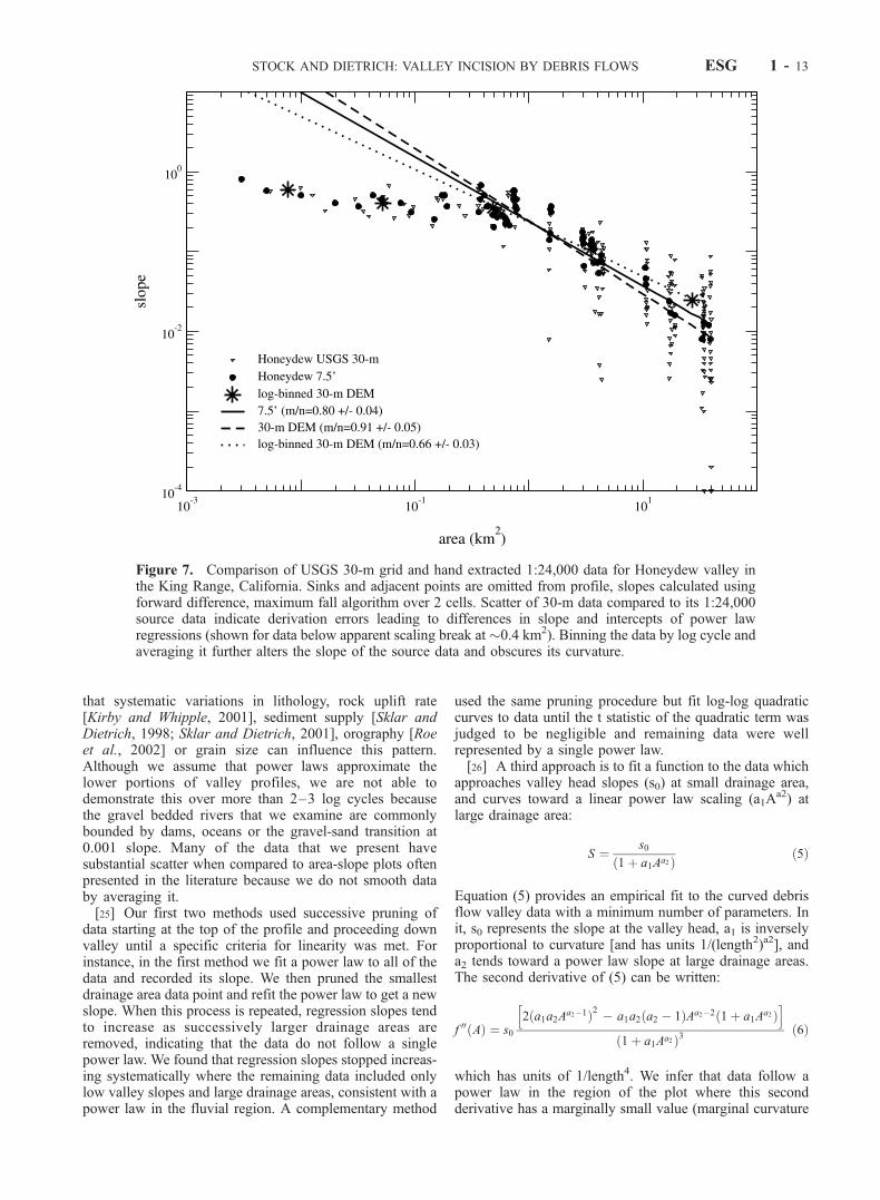
compares hand-measured area-slope data with 30-m DEMdata for a steep basin in the King Range, California. Weremoved sinks from the source 30-m data by increasing theelevation of such cells in 0.1 m increments. We extractedthe valley network with a threshold drainage area of 5 ormore cells, and removed cells that were influenced by sinks.Although the derivative 30-m data are similar to the contourdata in some respects (m/n values are almost within onestandard error), the scatter of the 30-m data obscures theregion in which the data change trend. It is this region thatdefines the extent of fluvial power law relations, and there-fore 30-m data are not adequate to resolve this issue.Although averaging by log-binning smoothes noise, it doesnot recreate the original data pattern.

4.1. Techniques for Hand Extraction ofArea-Slope Data

[23] We conclude that network extraction from 30-mDEMs in steeplands where valley bottoms are substantiallyless than 30 m wide introduces noise to the source data.Therefore, except for the laser altimetry, we measured mainstem valley area and slope by hand from contoured1:24,000 or 1:50,000 scale topographic maps. To makearea-slope plots for valleys in the laser altimetry coverage,we extracted the valley network using a simple thresholddrainage area of 1000 m2, which approximates the valleynetwork that we observe in the field here. We used amaximum fall algorithm for slope with a forward differenceof two grid cells, extracted the profile data, and binned andaveraged values over 10-m increments to smooth slopevariations from thick-bedded sandstone cliffs. For all othersites we measured slope and drainage area at a pointequidistant between elevation contours for every contourcrossing of the valley. We enlarged steep areas with closelyspaced contours 200% on a photocopier. Where contoursare closely spaced, we sampled area at every other contourinterval, measuring slope between adjacent contours. Wecalculated slope as the contour interval divided by the valleyblue-line distance, or if these are absent, the shortestdistance along valley between adjacent contours. We stop-ped collecting data near the drainage divide at the valleyhead, which we defined as the last segment where thecontour direction angle from one side of the valley to theopposite changes by �150� or less. This is a crude approx-imation for the actual hollow location, but we found it to bea rough measure of valley head location based on compar-ison of 1:24,000 maps to field observations of hollows inFigure 5. We used a polar planimeter to measure drainagearea, resulting in a precision of ±0.001 square inches (e.g.,3.7 10�4 km2 for 1:24,000 maps). Using a ruler tomeasure horizontal distance between contours results in aprecision of ±0.25 mm (6 m for 1:24,000 maps, 3 m for the200% enlargement). Corresponding point uncertainties inslope range from small fractions of a percent in the lowlandsto 50% in the steepest parts of the profile, although practicaluncertainties appear less than 20% on the basis of field andlaser altimetry comparison to contour maps.

4.2. Techniques to Extract Power Law Portion of Data

[24] We used three methods to identify potential fluvialpower law segments of main stem area-slope plots. All threeassumed that valleys carved by fluvial processes have area-slope data fit best by a power law, although we recognize


that systematic variations in lithology, rock uplift rate[Kirby and Whipple, 2001], sediment supply [Sklar andDietrich, 1998; Sklar and Dietrich, 2001], orography [Roeet al., 2002] or grain size can influence this pattern.Although we assume that power laws approximate thelower portions of valley profiles, we are not able todemonstrate this over more than 2–3 log cycles becausethe gravel bedded rivers that we examine are commonlybounded by dams, oceans or the gravel-sand transition at0.001 slope. Many of the data that we present havesubstantial scatter when compared to area-slope plots oftenpresented in the literature because we do not smooth databy averaging it.[25] Our first two methods used successive pruning of

data starting at the top of the profile and proceeding downvalley until a specific criteria for linearity was met. Forinstance, in the first method we fit a power law to all of thedata and recorded its slope. We then pruned the smallestdrainage area data point and refit the power law to get a newslope. When this process is repeated, regression slopes tendto increase as successively larger drainage areas areremoved, indicating that the data do not follow a singlepower law. We found that regression slopes stopped increas-ing systematically where the remaining data included onlylow valley slopes and large drainage areas, consistent with apower law in the fluvial region. A complementary method

used the same pruning procedure but fit log-log quadraticcurves to data until the t statistic of the quadratic term wasjudged to be negligible and remaining data were wellrepresented by a single power law.[26] A third approach is to fit a function to the data which

approaches valley head slopes (s0) at small drainage area,and curves toward a linear power law scaling (a1A

a2) atlarge drainage area:

S ¼ s0

1þ a1Aa2ð Þ ð5Þ

Equation (5) provides an empirical fit to the curved debrisflow valley data with a minimum number of parameters. Init, s0 represents the slope at the valley head, a1 is inverselyproportional to curvature [and has units 1/(length2)a2], anda2 tends toward a power law slope at large drainage areas.The second derivative of (5) can be written:

f 00 Að Þ ¼ s0

2 a1a2Aa2�1ð Þ2 � a1a2 a2 � 1ð ÞAa2�2 1þ a1A

a2ð Þh i

1þ a1Aa2ð Þ3ð6Þ

which has units of 1/length4. We infer that data follow apower law in the region of the plot where this secondderivative has a marginally small value (marginal curvature

Figure 7. Comparison of USGS 30-m grid and hand extracted 1:24,000 data for Honeydew valley inthe King Range, California. Sinks and adjacent points are omitted from profile, slopes calculated usingforward difference, maximum fall algorithm over 2 cells. Scatter of 30-m data compared to its 1:24,000source data indicate derivation errors leading to differences in slope and intercepts of power lawregressions (shown for data below apparent scaling break at �0.4 km2). Binning the data by log cycle andaveraging it further alters the slope of the source data and obscures its curvature.


technique) for parameter values from the fit to the full dataset.[27] The first two methods have the disadvantage that

endpoints (particularly those that are downstream) exert atremendous leverage on both m/n values in equation (4) andquadratic curvature. Even small deviations from linearity ona single downstream end point can lead to transition slopevalues well downstream of debris flow run outs (e.g.,<0.02). Therefore these methods can only be applied todata that follow a power law exceedingly well. The thirdmethod has the advantage of being very robust to scatter indata, but requires a judgment of the threshold curvature atwhich the function is well approximated by a line. There-fore we use a combination of these three techniques. Weused m/n and t statistics on data sets with well-definedlinear portions as judged by R2 values greater than 0.9 (boldm/n values in Table 3). Where m/n stopped increasingmonotonically and the t statistic indicated that there waslittle significance to a quadratic fit parameter (jtj < 1), weinferred a single power law. We then used these results tochoose a curvature value at which the second derivative ofequation (5) was judged to be vanishingly small, so that theremaining data approximate a power law. We call theupstream-most data point on the power law the river valleyhead.[28] For instance, Figure 8 shows all three methods

applied to Deer Creek, for data spanning its headwaters to

near the mouth of the main stem San Lorenzo at the PacificOcean (Figure 1b). The m/n value stops increasing system-atically where the t statistic approaches �1 at a drainagearea of �4 km2. The third line indicates curvature derivedfrom a Levenberg-Marquardt nonlinear fit to the data usingequation (5) with inverse slope weighting. Curvature valuesof �10�3 correspond to the transition to linearity as judgedby the previous two techniques. We fit (5) to each full dataset, and where its second derivative reaches 10�3 we inferthe beginning of a single power law. To characterize thecurvature of the data above the power law, we refit (5) todata above the threshold curvature value. For both fits, weweight each data point by the inverse of its slope, which isequivalent to weighting each data point by the valley lengthover which its slope is evaluated. Thus the more frequentdata from steeper portions of the profile have proportionallyless weight and do not bias the fit. This is comparable toweighting each DEM pixel equally along a profile, andreduces the influence of knickpoints or other short-lengthscale features on the fit.

5. Results

5.1. Curvature of Area-Slope Data

[29] In steepland valleys of the western United States wehave observed sediment removal and bedrock loweringalong the entire run out of 13 recent debris flows in Oregon,

Figure 8. Plot of three methods to extract power law portion of area-slope plot for Deer Creek (see text).The m/n value is the slope of a power law regression applied to the data when successively larger drainageareas are pruned away for each fit. Values converge when there is no systematic curvature in the data, sothat it approximates a single power law. The t statistic is a measure of the significance of a quadratic term ina nonlinear fit to the data using the same pruning. It falls to negligible magnitude (below 1) where m/nvalues converge (vertical dashed line) and where the curvature of equation (5) reaches 10�3. Together,these criteria indicate that Deer Creek has a single power law at drainage areas larger than �4 km2.


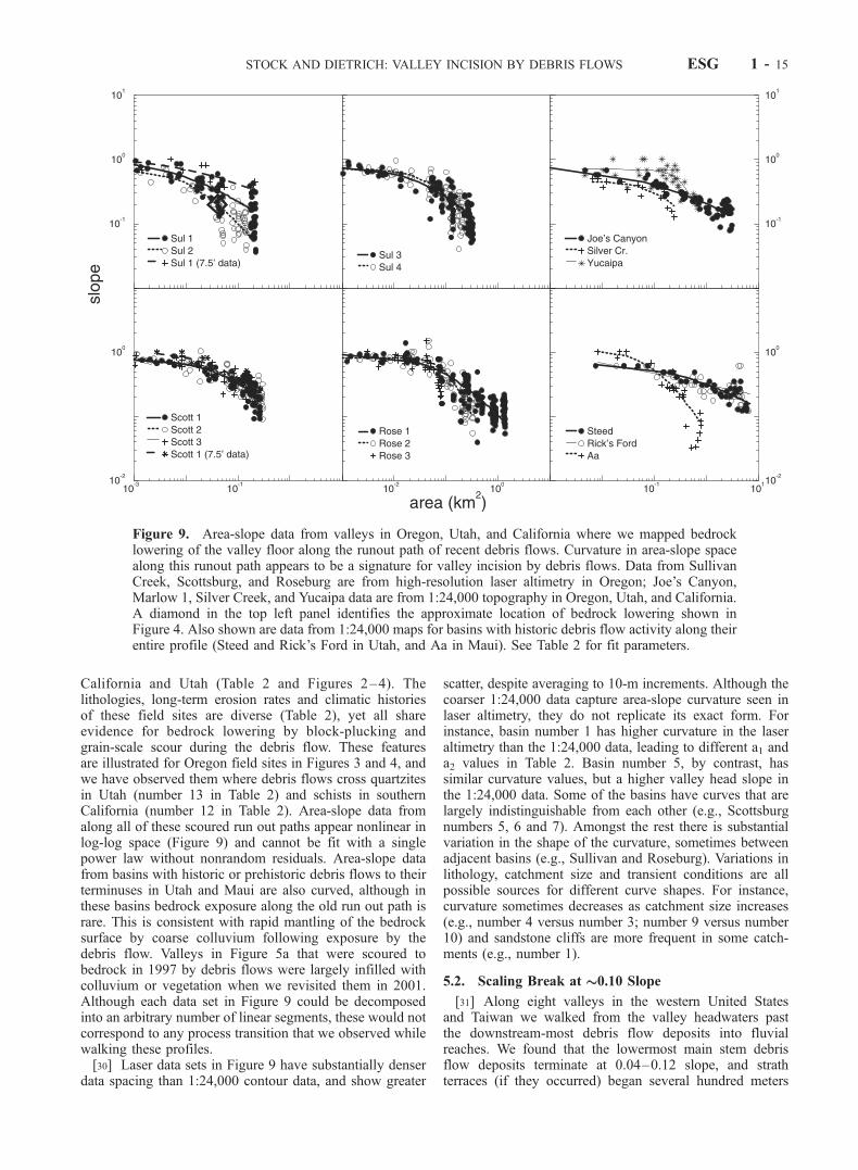
California and Utah (Table 2 and Figures 2–4). Thelithologies, long-term erosion rates and climatic historiesof these field sites are diverse (Table 2), yet all shareevidence for bedrock lowering by block-plucking andgrain-scale scour during the debris flow. These featuresare illustrated for Oregon field sites in Figures 3 and 4, andwe have observed them where debris flows cross quartzitesin Utah (number 13 in Table 2) and schists in southernCalifornia (number 12 in Table 2). Area-slope data fromalong all of these scoured run out paths appear nonlinear inlog-log space (Figure 9) and cannot be fit with a singlepower law without nonrandom residuals. Area-slope datafrom basins with historic or prehistoric debris flows to theirterminuses in Utah and Maui are also curved, although inthese basins bedrock exposure along the old run out path israre. This is consistent with rapid mantling of the bedrocksurface by coarse colluvium following exposure by thedebris flow. Valleys in Figure 5a that were scoured tobedrock in 1997 by debris flows were largely infilled withcolluvium or vegetation when we revisited them in 2001.Although each data set in Figure 9 could be decomposedinto an arbitrary number of linear segments, these would notcorrespond to any process transition that we observed whilewalking these profiles.[30] Laser data sets in Figure 9 have substantially denser

data spacing than 1:24,000 contour data, and show greater

scatter, despite averaging to 10-m increments. Although thecoarser 1:24,000 data capture area-slope curvature seen inlaser altimetry, they do not replicate its exact form. Forinstance, basin number 1 has higher curvature in the laseraltimetry than the 1:24,000 data, leading to different a1 anda2 values in Table 2. Basin number 5, by contrast, hassimilar curvature values, but a higher valley head slope inthe 1:24,000 data. Some of the basins have curves that arelargely indistinguishable from each other (e.g., Scottsburgnumbers 5, 6 and 7). Amongst the rest there is substantialvariation in the shape of the curvature, sometimes betweenadjacent basins (e.g., Sullivan and Roseburg). Variations inlithology, catchment size and transient conditions are allpossible sources for different curve shapes. For instance,curvature sometimes decreases as catchment size increases(e.g., number 4 versus number 3; number 9 versus number10) and sandstone cliffs are more frequent in some catch-ments (e.g., number 1).

5.2. Scaling Break at ��0.10 Slope

[31] Along eight valleys in the western United Statesand Taiwan we walked from the valley headwaters pastthe downstream-most debris flow deposits into fluvialreaches. We found that the lowermost main stem debrisflow deposits terminate at 0.04–0.12 slope, and strathterraces (if they occurred) began several hundred meters

Figure 9. Area-slope data from valleys in Oregon, Utah, and California where we mapped bedrocklowering of the valley floor along the runout path of recent debris flows. Curvature in area-slope spacealong this runout path appears to be a signature for valley incision by debris flows. Data from SullivanCreek, Scottsburg, and Roseburg are from high-resolution laser altimetry in Oregon; Joe’s Canyon,Marlow 1, Silver Creek, and Yucaipa data are from 1:24,000 topography in Oregon, Utah, and California.A diamond in the top left panel identifies the approximate location of bedrock lowering shown inFigure 4. Also shown are data from 1:24,000 maps for basins with historic debris flow activity along theirentire profile (Steed and Rick’s Ford in Utah, and Aa in Maui). See Table 2 for fit parameters.


down valley from these deposits (Figure 10). Area-slopedata up valley from these mapped terminal debris flowdeposits (open symbols) are curved in the same manner asdata from basins where we recorded bedrock scour fromdebris flows (e.g., Figure 9). For instance, Figure 11bshows residuals from two power law fits to Deer Creekshown in Figure 11a, the entire data set and a subset ofslopes greater than 0.10 (location of recent debris flowdeposits). For both fits, positive residuals occupy themiddle of the plot, negative residuals the ends. Neitherthe whole plot, nor the steep portion where we havemapped modern debris flows can be fit with a singlepower law.[32] Valley slopes downstream of the first strath terrace

approximate a linear power law (solid symbols) as judgedby a marginal curvature technique. For instance, strathterraces in Deer, Noyo, Honeydew and Elder Creeks mapdownstream of the beginning of the power law. In Bear,straths are absent, but the beginning of the power law regioncorresponds to the appearance of large potholes and runnelsin the granite-floored channel. The extension of power lawscaling above this transition region substantially over-pre-dicts valley slope at low drainage areas (Figure 10) and is

therefore a poor approximation for steeper valley slopes.Marlow and Sullivan Creek basins are smaller than ourother examples and may not have enough data to define apower law, particularly with knickpoints that obscure poten-tial trends. Curvature for these basins is lower than higher-resolution laser altimetry indicates for adjoining basins, butstill present in 1:24,000 data.[33] Above the end of the power law and the upstream-

most strath terraces of the valleys in Figure 10, we observedevidence that reaches transition from fluvial to debris flowactivity over several hundred meters or more. In them, weobserved fluvial bed forms (commonly step-pools) and fillterraces, but also occasional debris flow deposits. InAnghou, Deer, Honeydew, Elder and Bear, step-pools andrare debris flow deposits of the transition reaches gave wayupstream to boulder cascades that filled the valley. In somebasins, the slopes of these transition reaches are smaller thanthose found further downstream (e.g., Noyo, Deer, andHoneydew basins) but increase rapidly upstream oncedebris flow deposits become common. Valleys upstreamof the transition region are straight or broadly curved inplanform, but lack the repetitive meandering seen in rivers.If present, fill terraces were commonly bouldery debris flow

Figure 10. The extent of debris flows along the main stem as estimated by preserved deposits (opensymbols) mapped in the field onto 1:24,000 topography. The zone of departure from the fluvial powerlaw lies near the downstream end of existing debris flow deposits and upstream from last observed strathterrace. Extension of single power law (shown by lines) substantially overestimates valley slope at lowdrainage areas (see text for methods used to define linear portion of data). Data for each basin is boundedat its downstream end by presence of the ocean (Noyo, Taiwan, Deer, Honeydew, Marlow, and Sullivan)or dams (Bear). Sullivan and Marlow Creeks lack defined power law scaling because of a combination ofknickpoints and small drainage areas. They illustrate the importance of using sufficiently large basins todefine fluvial trends.


deposits that had been partially incised. Bedrock exposuresalong the valley floor were restricted to a few waterfalls.

5.3. Extension to Other Steeplands

[34] The scaling break that we observe in Figure 10 alsooccurs in steepland basins in the United States (Figure 12a)and around the unglaciated world (Figure 12b). At largerdrainage areas, the slopes of many of these basins approx-imate a power law (e.g., Djemaa, Vistula, Golema, Deer,Noyo, Bear, Indian and Honeydew basins). Although thereis significant scatter in some of the basins (e.g., Nam Se,Trapachillo, Simbolar), projection of power laws to smalldrainage areas would not predict valley head slopes sub-stantially in most cases (e.g., Figure 10). The sole exceptionis a mudstone basin from Italy (Marecchia) that may havebadlands dominated by overland flow in its headwaters (M.Casedei, UCB Earth and Planetary Science, personal com-munication, 2002).[35] We extracted the power law portion of the data for

most of the basins in Figure 12 (except Marecchia, Marlowand Sullivan) using marginal curvature techniques with

equation (6) and then fit nonlinear data up valley (usuallyincluding transition reaches discussed above) with equation(5). Table 3 summarizes parameters from fluvial power lawfits including the slope (m/n) and intercept {[(�@z/@t)/K]1/n},as well as parameters from the fit of equation (5) to dataabove the power law region. Also shown are the approx-imate slopes and drainage areas at the transition, elevationsof valley and river valley heads on the source contour map,and the fraction of valley relief within the debris flowregion.[36] This fraction is defined as elevation difference

between valley head and scaling transition point (river head)divided by the elevation of drainage divide. We used the lastdrainage area in the debris flow region, and the first in thepower law region to bracket the drainage area of the scalingtransition. We estimated the slope values at the transition byusing the lowest debris flow slopes and the highest riverslopes around the transition. Where rivers have locally steepslopes (e.g., Simbolar, Jellamayo) or debris flows havelocally low slopes (e.g., Knawls, Indian), these values areincluded, leading to substantial ranges.[37] We found that valley slopes begin to fall system-

atically below the fluvial power law prediction as theyapproach values from 0.03–0.10 (see scaling transitionscolumn in Table 3), similar to results from Figure 10. Justabove the river head, there is commonly a short regionwhere slope increases more rapidly than anywhere else onthe plot (e.g., Honeydew, Deer, Djemaa, Nam Se, St.Germain, Ter, and Simbolar). This occurs where thecurved data do not join the power law fluvial trendasymptotically. Above this high curvature region, there iscommonly a more gentle curvature as the valley head isapproached. The magnitude of curvature (approximated bya1 in Table 3) varies widely among basins. Grouping thebasins by map scale, and by lithology and erosion rate canreduce the variation. For instance, for the last 12 U.S.basins dominated by sedimentary rocks in Table 3, a plotof erosion rate against a1 in log-log space shows a roughcorrelation (R2 = 0.77) with curvature increasing witherosion rate. Global data in basins of sedimentary rock(excluding the Marecchia and basins with combinations ofclastics and metamorphic rocks) show a similar relation,although they are more scattered (R2 = 0.70). Basins withcrystalline rocks on the other hand tend to have lowercurvature for similar erosion rates. For instance, at erosionrates between 0.1–0.3 mm/yr, Djemaa and Toplodolskabasins cut in sedimentary rocks have lower a1 values (thushigher curvature) than Simbolar, Chasong-gang and Jella-mayo basins, which are cut in granites and gneisses.Because a1 trends with erosion rate and lithology are weakenough to be challenged, and the erosion rates for many ofthe basins have large but unquantifiable uncertainties, amore focused effort is required to evaluate these correla-tions with lithology and erosion rate.[38] Figure 12 and s0 values in Table 3 illustrate that these

valleys heads approach slopes of 0.3–1, and more com-monly slopes of 0.4–0.5, over a wide range of lithology anderosion rates. Comparison of 1:50,000 to 1:5,000 data forthe same basin (upper-left panel in Figure 12b) indicate thatcoarser topography captures a smoothed version of finer-resolution data, so curvature from 1:50,000 scale maps isnot an artifact of coarse scale.

Figure 11. (a) Plot of Deer Creek, Santa Cruz Mountains.Extension of a fluvial power law to steep valleys isinappropriate, as shown by nonrandom residuals. Also notethat the trend at small drainage areas is nonlinear.Catchment bedrock is sandstone, erosion rates are 0.15–0.3 mm/yr (see text for details). (b) Absolute values ofdifferences between predicted and observed slopes in Figure11a show a nonrandom pattern indicating that only thelower fluvial section is linear.


[39] Below the scaling break, the exponents of the powerlaw regression vary substantially, from near zero values to1.4 (Table 3). Basins with power law fits whose R2 isgreater than 0.9 are shown in bold, and those with R2 lessthan 0.7 are italicized. The former have m/n values from�0.7 to 1.0 for sedimentary and metamorphic lithologies.Basins with intermediate R2 values have a greater range ofm/n, from �0.5–1.4. Many low R2 values result from local,steep down valley reaches that disrupt a power law trend(e.g., Big Creek, Sandymush and Toplodolska) or pervasivescatter so that linear trends are less obvious (e.g., Nam Se,Simbolar, Jellamayo, and Trapachillo). Power laws fits tothe latter basins have low slopes whose upstream projec-tions intersect data above the river valley head, but do so inregions where data actually curve.

6. Discussion

[40] Four categories of observations indicate that debrisflows carve the bedrock of some steepland valleys, produc-ing a distinctive area-slope topographic signature: (1) fieldobservations of bedrock lowering caused by debris flows,(2) area-slope curvature in valleys with observed debrisflow bedrock lowering, (3) scaling break near terminaldebris flow deposits, up valley from straths (if they occur),and (4) scaling break in U.S. and global data near typicaldebris flow run out slopes of �0.03–0.10.[41] First, field observation along recent debris flow run

outs indicates that where bedrock is exposed, there isevidence for lowering caused by the debris flow. Thelowering is of sufficient magnitude to be geomorphicallyrelevant (e.g., Figure 4), although its style varies withlithology. Debris flows appear to be the dominant processexposing bedrock in steepland valleys whose floors areoften mantled with very coarse particles. Headwater valleysthat have not had recent debris flows (e.g., those in Figure10) lack or have only rare exposures of bedrock above step-pool reaches in slope ranges where debris flows occur. Therapid mantling of valleys in Oregon that were scoured tobedrock in 1997 also indicates that debris flows here may bethe only process capable of transporting away coarsematerial that accumulates rapidly in valley bottoms fromhillslope processes. Although sediment in valleys in Figures2 and 3 may eventually acquire a thin veneer of fluviallysorted sediment, it is usually colluvium below the surface[see also Benda, 1990; Benda and Dunne, 1997]. Transportof colluvium by concentrated flow following debris flows isalso reported [Larsson, 1982], but we know of no evidencefor bedrock lowering by concentrated flow following debrisflows. Although fluvial incision may be possible in this kindof circumstance, debris flows appear to be required just toexpose most of the valley floor bedrock.[42] Second, valleys where we have mapped scour (e.g.,

Figures 5a and 5b) have area-slope plots that curve in log-log space (Figure 9) throughout the overlapping regions ofobserved bedrock lowering and debris flow run out.Although there is much local scatter in high-resolutionOregon slope data due to alternation between sandstone

and siltstone beds, linear power laws will not fit the high-resolution topography of these valleys. This curvature isalso apparent on coarser-resolution data (e.g., 1:24,000 datain Figure 9), although we suspect that its exact parameter-ization requires higher-resolution data because Marlow andSullivan Creek plots (Figure 9) show different curvature.We propose that although the valley networks shown inFigures 2 and 5 closely resemble fluvial networks in plan-form, they are predominately carved by the entirely differentprocess of debris flow incision, whose signature is curvaturein log A-log S space.[43] Third, we find that a scaling break in the 1:24,000

area-slope data occurs approximately where identifiabledebris flow deposits end and strath terraces begin (e.g.,Figure 10). This transition in process is mirrored in thetopography as a scaling break in valley area-slope datawhen plotted in log-log space. We interpret the regionbetween frequent debris flow deposits and the beginningof strath terraces as a transition between fluvial bedrockincision and debris flow incision. Although these reachesare likely a combination of processes, we include their fewdata points in the debris flow region because their up valleyextent is difficult to estimate.[44] Fourth, analysis of many unglaciated steepland val-

leys in the United States and around the world indicates ascaling break from data that could be modeled with a singlepower law to data that are nonlinear in log-log space (Table3) near where field observations (e.g., Tables 1 and 2)indicate that debris flows deposit (slopes > 0.03). Sincemany rivers lack strath terraces (e.g., Bear River), there aresubstantial uncertainties in the long-term boundary betweenfluvial and debris flow valley incision. Therefore thetransition boundaries listed in Table 3 for valleys that wehave not walked should be regarded as illustrative ratherthan definitive.[45] Transient changes in valley long profile or system-

atic variations in rock uplift rate [Kirby and Whipple, 2001]or lithology may also have their own signature on area-slopeplots. We have tried to minimize these effects by careful siteselection, but we cannot demonstrate that all of our siteshave topography at steady state. Some are likely to be out ofequilibrium at some time or space scale. For instance, basinswhose data are poorly fit with power laws in fluvial regions(e.g., Nam Se, Simbolar, Jellamayo, and Trapachillo) mayhave transient knickpoints that lower m/n values. Althoughfluvial power laws do not overestimate some slopes aboveriver valley heads in these basins, they also do not capturecurvature above the river valley head. What we find con-vincing is that across a wide range of rock uplift rates andlithologies, the scaling break takes place at around 0.03–0.10, the lowest slopes that many field studies indicate thatlarger debris flows can reach (e.g., Table 1).[46] While the evidence that we have acquired points

toward the dominant role that debris flows play cuttingsteepland valleys, it does not mean that all valleys greaterthan 0.03–0.10 slope are cut solely by debris flows. Inlandscapes without mass failures (e.g., some badlands),overland flow may still predominate. Nor have we estab-

Figure 12. (opposite) Data from unglaciated steepland valleys (a) in the United States (1:24,000) and (b) around the world(1:50,000). Note that extension of linear power law trends of large drainage areas would tend to overpredict valley slopeabove 0.10 across a wide range of climate, rock uplift rates, and lithology. See Table 3 for details.


lished that fluvial processes play no role in steepland valleyincision. Rather, we find that the tendency for rapid burialof valley floors after debris flows precludes the widespreadoccurrence of fluvial incision along debris flow run outs. Infield areas where sediment cover is absent and flow occurs,fluvial incision at steep slopes might give rise to a differentsignature (e.g., Marecchia).

6.1. Implication of Scaling Transition

[47] Large fractions of valley relief (25–75%) lie abovethe scaling break at the river valley head for basins that weinvestigated in Table 3, in reaches steep enough to transportdebris flows. Although increasing basin size and distancefrom base-level (hence average slope) reduce this fraction, itis still substantial even for large basins far away from coasts(e.g., Toplodolska, Vistula, St. Germain). In steep rangesnear the coast (e.g., Honeydew, Franklin, Anghou), debrisflow valleys are the dominant portions of valley relief(>70%). The location of the transition near the end of debrisflow run outs is consistent with a threshold slope beyondwhich debris flows are not mobile and cannot incise valleys(e.g., Tables 1 and 2). Using 0.10 valley slope as aconservative estimate for this limit, we find that in steep-lands like the Oregon Coast Range, most of the valleynetwork by length, and large fractions of it by relief (Table 3)

are cut by debris flows, not rivers. Figure 13 illustrates this inthe 100-km2 Millicoma basin (from a 10-m DEM kindlyprovided by Stephen Lancaster, Oregon State University,Corvallis, OR), cut in the Tyee Formation of the OregonCoast Range. In blue are 10-m valley segments of less than0.10 slope, a maximum estimate for the extent of fluvialincision. Nonetheless, the red valley network of >0.10 slopesoccupies nearly 90% of the channel network length, includ-ing much of the local relief. The image indicates that most ofthe hillslopes in this basin have boundary lowering rates thatare set predominately by debris flow incision, not fluviallowering, and that much of the landscape relief resides invalleys cut by debris flows.[48] Figure 14 shows profiles for three basins where we

have identified process transitions in the field and scalingbreaks on area-slope plots. The scaling break in the area-slope plots for each basin occurs at the intersection of thedashed lines with the existing long-profile (solid line). Abovethe intersection, the valley has a curved area-slope plot thatwe infer represents debris flows incision. For these basins,debris flow portions of the main stem valley occupy 40–80%of the main stem relief. The dashed lines represent what theprofile would look like if the fluvial power law scaling of thelower part of the plots (Figure 10) extended to the valley headdefined by contour direction angle. They indicate the role that

Figure 13. Valley network of the 100-km2 Millicoma basin, Oregon, extracted from a 10-m DEM. At adrainage area threshold of 1000 m2, 90% of the valley network length is above 0.10 gradients wheredebris flows are known to occur.


debris flows have in controlling existing valley relief,although other processes like deep-seated landsliding wouldprobably occur before valleys reached these extreme slopes.[49] Figure 14 and the fraction of valley relief above river

valley heads (Table 3) illustrate that a debris flow incision law,as yet unknown, determines much of the main stem relief andmost of the tributary relief for unglaciated steeplands. Thismeans that there is much yet to be learned about the evolutionof steep escarpments, river valleywalls, and the persistence oftopography in orogens, all of which are commonly charac-terized by valleys with slopes greater than 0.10. Likewise, theinfluence of climate and erosion rate on relief will requiresome assessment of the role of debris flows. The transitionzone between fluvial and debris flow valley incision, wheredebris flow material accumulates in the short term, alsoremains a problematic region aboutwhichweknowvery little.

6.2. Interpretation of Curvature

[50] Fits of equation (5) to U.S. and global debris flowvalley profiles have substantial variability, as shown by therange of parameters in Tables 2 and 3. Some of the variationis likely a size effect, with smaller catchments having highercurvature as their longitudinal profiles curve rapidly to joinmain stems. This size effect in itself indicates that equation(5) does not adequately capture all of the relevant effectscontrolling curvature.[51] Other variations in area-slope curvature may reflect

response to boundary lowering rates. For instance, catch-ments on either side of the knickpoint in Sullivan Creekhave different curvature (e.g., number 1 versus number 2 in

Table 2) that may reflect a transient response. Steady stateresponses to rock uplift rates and lithology may alsoinfluence curvature.[52] For instance, Figure 15 summarizes hypotheses

about valley response to variations in rock uplift rate andlithology, based on inverse correlation between a1 anderosion rate that we observe for some basins of similarlithology in Table 3. Valleys cut by debris flows are shownas dashed lines and solid lines show river-cut valleys. Whileriver valleys follow a power law that translates upward withrock uplift rate, debris flow valley slopes in Figure 15aconverge to an upper limit within the range of slopescommonly reported for hollows in soil-mantled landscapes.By visual analogy to the string of a bow, Figure 15 showsthe debris flow curve pulled upwards and toward greaterdrainage areas as erosion rates increase, but pinned belowslopes at which landslides initiate. This is consistent withthe observation that in most of the basins in Figure 12,valley heads reach a limiting slope at vanishingly smalldrainage areas that is seemingly insensitive to rock upliftrate. This value is near the friction angle for many soils, andis likely set by landslide initiation at hollows, 20–100 mbelow the ridgeline in our examples. We cannot say whetherthe upper threshold slope is set by material properties, or themaintenance of slopes above which debris flow incision isextraordinarily rapid. At the other end of the profile, thebowstring is pinned by the lowermost slope values at whichdebris flows tend to deposit in confined valleys, often slopesof 0.03–0.10. Here there is occasionally an abrupt increasein slope at the upstream end of the linear fluvial trend (see

Figure 14. Plot of profiles from Bear, Honeydew, and Deer Creek indicating that much of the valleyrelief lies in debris flow region. Shown for comparison are profiles predicted by extending slopespredicted by river incision law to valley head (defined by planform curvature from topographic maps).


for instance Deer, Cook, Djemaa) leading to a profilesteepening at the river valley head.[53] As rock uplift rates increase, we hypothesize that

there is a tendency for lower threshold slopes to migrate tosuccessively larger drainage areas (e.g., Yucaipa, Honey-dew). Similar tendencies have been predicted for fluvialsystems by the models of Howard [1997] and Tucker andBras [1998]. For debris flow cut valleys, this would focusboth long-profile and area-slope curvature in the remainingregion above the river valley head, resulting in nearly linearupper long-profiles that curve rapidly concave upwardsapproaching the river valley head. This region of responseto rock uplift rates is consistent with the finding by Merritsand Vincent [1989] that first order channels respond mostsensitively to rock uplift rates, because their blue-line firstorder channels occur at drainage areas of �0.1 to 1 km2,within the highly curved lower section of debris flow area-slope data where small changes in curvature lead to largechanges in slope. For the purposes of illustrating thishypothesis, we compare area-slope data from predominatelysandstone basins with erosion rates ranging from �0.01 to4 mm/yr (Figure 16a). For these basins, area-slope data aremore curved at high erosion rates (e.g., Honeydew Creek)compared to low erosion rates (e.g., Knawls Creek, West

Virginia). Hypothetical differences between tectonicallyactive areas and passive ones can also be illustrated bycomparing granite basins with little active tectonism(Korea) to those with high erosion rates (San Gabriels) inFigure 16b. Here again there is higher curvature in thedebris flow region where erosion rates are higher.[54] We hypothesize that there is also an influence of

lithology on valley profile. Figure 17 illustrates that forroughly equivalent erosion rates, valleys in crystallinerocks like gneisses and granites may be steeper for a givendrainage area than those cut in sandstones. Valleys incrystalline rocks or indurated rocks like basalts may alsotend to have lower curvatures in the debris flow region (asreflected in larger a1 values in Table 3) than valleys insedimentary rocks for similar erosion rates (Figures 17aand 17b).

6.3. Implications for Stream Power Law Exponents

[55] Our comparisons of USGS 30-m data to hand-extracted 1:24,000 data and to laser altimetry indicate thatscatter in the 30-m data obscure scaling transitions and donot exactly reproduce source data parameters (e.g., m/n

Figure 16. Apparent effect of rock uplift rates on valleyslope in (a) sandstone basins, Knawls Creek, (WestVirginia) and Deer Creek, Santa Cruz Mountains, andHoneydew (California), and (b) granitic basins, Chasong-gang, North Korea, and Bear Creek, San Gabriels,California. Solid symbols are data that follow a fluvial,linear power law (see text for details). Open symbols arecurved, reflecting debris flow valley incision. See Table 3for fit parameters.

Figure 15. Hypothetical response of valley network tovariations in rock uplift rate/rock resistance ratio. As rockuplift rates increase, river valley slopes (solid lines) increaseas intercept of the power law translates upward. Debris flowvalley slopes (dashed lines) also become steeper resulting ina more linear long profile.


values). At low drainage areas (e.g., <10�4 km2) much of thenetwork may be artifactual, while at larger areas slope scatteris substantial. Therefore 30-m DEMs used for area-slopeanalysis need to be validated by comparing them to the1:24,000 quadrangle source before they can be used to inferscaling laws. Great care should be taken to ensure that the databeing fit with power laws are indeed linear in log-log space.For instance, inclusion of data that curve at low drainage areasin power law regressions decreases m/n values and increasesintercept [(�@z/@t)/K]1/n values (e.g., Figure 7). This couldlead to spurious correlations between rock uplift rate andpower law slope and intercept. To avoid this problem, head-water reaches above 0.03 slope should be excluded fromstream power law analysis unless they are demonstrablyinfluenced by fluvial incision (e.g., presence of strath terracesor extension of well-defined single power law).[56] Even m/n values extracted only from fluvial regions

vary substantially in Table 3. For instance, basins thatfollow a single power law exceedingly well (R2 values >0.9) have m/n values that vary from 0.7–1.0 for sedimen-

tary and metamorphic lithologies. Valleys in hard, crystallinerocks like granites tend to have m/n values (0.4–0.6) lowerthan those of valleys in sedimentary rocks, but this might alsobe an artifact of the small number of valleys we measured ingranitic rocks. The range of m/n values in Table 3 spans thosereported in the literature, from high values like 1.0 [Seidl andDietrich, 1992; Seidl et al., 1994], to lower values like 0.1–0.5 [Stock and Montgomery, 1999; Snyder et al., 2000]. Wehave not established that each basin has uniform lithology oris at steady state, but this variation in m/n indicates that thereis no single m/n value that can be extracted from topographicdata for a general stream power law.

7. Conclusions

[57] Field observations and map analysis demonstrate thatdebris flows that occur in landscapes steep enough toproduce mass failures both erode bedrock and have atopographic signature in the form of curvature in area-slopespace above 0.03–0.10 slope. Power law plots of slopeversus area, widely used to examine bedrock river incisionlaws, begin to over-predict valley slopes just upstream ofthe last strath terrace. Above this region, the influence ofdebris flows increases rapidly, and is reflected in a curvedrelation between slope and area on log-log plots thatcorresponds to mapped debris flow run outs. This topo-graphic signature is consistent with a fundamentally differ-ent valley incision law by debris flows, whose form wefurther explore in a forthcoming paper. Much of the world’ssteepland valleys, similar in planform appearance to fluvialnetworks, may be cut by debris flows. Debris flow networksare relevant to landscape evolution because they are bothextensive by length (>80% of large steepland basins) andcomprise large fractions of main stem valley relief (25–100%). As a consequence, valleys that are predominatelycarved by debris flows, not rivers, bound most hillslopes inunglaciated steeplands. Debris flows limit the relief ofunglaciated mountain ranges to substantially lower eleva-tions than river incision laws would predict. Together theseobservations demonstrate that a debris flow incision law isneeded to explore mechanistic linkages between tectonics,climate, and topography in unglaciated steeplands.

[58] Acknowledgments. Initial work by Michelle Seidl and DavidMontgomery on area-slope breaks encouraged our analysis of area-slopedata. Douglas Allen and Dino Bellugi taught the senior author Arc/Info, andJim Kirchner helped with the analysis of curved versus linear data. Wethank Stephen Lancaster for sharing 10-m DEMs of the Elliot State Forest.Chad Pedriolli did some of the area-slope measurements. We thank thefollowing for field assistance: Simon Cardinale, Mauro Cassidei, TeganChurcher, Alex Geddes-Osborne, Meng-Long Hsieh, Cliff Riebe, JoshRoering, Kevin Schmidt, Leonard Sklar, Adam Varat, and Elowyn Yager.Reviews by Michael Singer, Greg Tucker and Stephen Lancaster improvedthe manuscript. This research was supported by NASA grant NAG 59629.

ReferencesAlford, D., Streamflow and sediment transport from mountain watershedsof the Chao Phraya basin, northern Thailand: A reconnaissance study,Mountain Res. Dev., 12, 257–268, 1992.

Anderson, R. S., Evolution of the Santa Cruz Mountains, California,through tectonic growth and geomorphic decay, J. Geophys. Res., 99,20,161–20,179, 1994.

Ando, N., K. Terazono, and R. Kitazume, Sediment removal project atMiwa dam, paper presented at Dix-huitieme Congres des Grandes Bar-rages, Comm. Int. des Grands Barrages, Durban, South Africa, 1994.

Armstrong, P. A., T. A. Ehlers, D. S. Chapman, K. A. Farley, and P. J. J.Kamp, Exhumation of the central Wasatch Mountains: Constraints from

Figure 17. Apparent effect of lithology on valley form.Solid symbols are data that follow a fluvial, linear powerlaw (see text for details). Open symbols are curved,reflecting debris flow valley incision. See Table 3 forparameters of both fits. Valleys in crystalline or induratedrocks (e.g., some basalts) tend to have lower long-profilecurvature in both fluvial and debris flow regions. This isreflected in lower m/n values for granites and basalts versussandstones at similar rock uplift rates, and higher values ofa1 in the debris flow region (indicating lower curvature) forcrystalline rocks and basalts versus sandstones.


low-temperature thermochronometry, Eos Trans. AGU, 80 Fall Meet.Suppl, F1034 1999.

Bagnold, R. A., An approach to the sediment transport problem from gen-eral physics, U.S. Geol. Surv. Prof. Pap., 422-I, 1966.

Benda, L. E., The influence of debris flows on channels and valley floors inthe Oregon Coast Range, U.S.A., Earth Surf. Processes, 15, 457–466,1990.

Benda, L., and T. W. Cundy, Predicting deposition of debris flows inmountain channels, Can. Geotech. J., 27, 409–417, 1990.

Benda, L., and T. Dunne, Stochastic forcing of sediment supply to channelnetworks from landsliding and debris flows, Water Resour. Res., 33,2849–2863, 1997.

Berti, M., R. Genevois, A. Simoni, and P. R. Tecca, Field observations of adebris flow event in the Dolomites, Geomorphology, 29, 265–274, 1999.

Blythe, A. E., D. W. Burbank, K. A. Farley, and E. J. Fielding, Structuraland topographic evolution of the central Transverse Ranges, California,from apatite fission-track, (U-Th)/He and digital elevation model ana-lyses, Basin Res., 12, 97–114, 2000.

Brown III, W. M., Erosion processes, fluvial sediment transport, and reser-voir sedimentation in a part of the Newell and Zayante Creek basins,Santa Cruz County, California, U.S. Geol. Surv. Open File Rep., 73-35,1973.

Campbell, R. H., Soil slips, debris flows, and rainstorms in the SantaMonica Mountains and vicinity, southern California, U.S. Geol. Surv.Prof., 851, 1975.

Carter, A., D. Roques, and C. S. Bristow, Denudation history of onshorecentral Vietnam: Constraints on the Cenozoic evolution of the westernmargin of the South China Sea, Tectonophysics, 322, 265–277, 2000.

Cenderelli, D. A., and J. S. Kite, Geomorphic effects of large debris flowson channel morphology at North Fork Mountain, eastern West Virginia,USA, Earth Surf. Processes Landforms, 23, 1–19, 1998.

Coats, R., L. Collins, J. Florsheim, and D. Kaufman, Landsliding, channelchange, and sediment transport in Zayante Creek and the lower SanLorenzo River, 1982 water year, and implications for management ofthe stream resource, report, State Water Resources Control Board, WaterResour. Cent. Archive, U. C. Berkeley, 1982.

Coltorti, M., and C. D. Ollier, Geomorphic and tectonic evolution of theEcuadorian Andes, Geomorphology, 32, 1–19, 2000.

Coltorti, M., and P. Pieruccini, A late Lower Miocene planation surfaceacross the Italian Peninsula: A key tool in neotectonic studies, J. Geo-dyn., 29, 323–328, 2000.

Costa, J. E., Physical geomorphology of debris flows, in Developments andApplications of Geomorphology, edited by J. E. Costa and P. J. Fleisher,Springer-Verlag, New York, 1984.

Curry, R. R., Observation of alpine mudflows in the Tenmile Range, centralColorado, Geol. Soc. Am. Bull., 77, 771–776, 1966.

Davis, W. M., River terraces in New England, Bull. Mus. Comp. Zool., 38,281–346, 1902.

Davy, P., and A. Crave, Upscaling local-scale transport processes in large-scale relief dynamics, Phys. Chem. Earth A, 25, 533–541, 2000.

Dendy, F. E., and W. A. Champion, Sediment deposition in U. S. reservoirs,Summary of data reported through 1975, U.S. Dep. Agric. Misc. Publ.,1362, 1978.

Dietrich, W. E., and T. Dunne, Sediment budget for a small catchment inmountainous terrain, Z. Geomorphol. Suppl., 29, 191–206, 1978.

Errih, M., and H. Bendahou, Desilting of water reservoirs in Algeria bydredging, study case: The Fergug reservoir, in Energy and Water: Sus-tainable Development, Proceedings of Theme D, 27th Congress of theIAHR, pp. 132–137, Am. Soc. of Civ. Eng., New York, 1997.

Fannin, R. J., and T. P. Rollerson, Debris flows: Some physical character-istics and behaviour, Can. Geotech. J., 30, 71–81, 1993.

Flint, J. J., Stream gradient as a function of order, magnitude, and discharge,Water Resour. Res., 10, 969–973, 1974.

Gay, I., and J.-J. Macaire, Estimation of late glacial and Holocene chemicalerosion rates, Lake Chambon watershed, Massif Central, France, Surf.Geosci., 328, 387–392, 1999.

Gilbert, G. K., Report on the Geology of the Henry Mountains, U.S. Gov.Print. Off., Washington, D. C., 1877.

Heimsath, A. M., W. E. Dietrich, K. Nishiizumi, and R. C. Finkel, Stochas-tic processes of soil production and transport: Erosion rates, topographicvariation, and cosmogenic nuclides in the Oregon Coast Range, EarthSurf. Processes Landforms, 26, 531–552, 2001.

Horton, R. E., Erosional development of streams and their drainage basins;hydrophysical approach to quantitative morphology, Geol. Soc. Am.Bull., 56, 275–370, 1945.

Howard, A. D., A detachment-limited model of drainage basin evolution,Water Resour. Res., 30, 2261–2285, 1994.

Howard, A. D., Badland morphology and evolution: Interpretation using asimulation model, Earth Surf. Processes Landforms, 22, 211–227, 1997.

Howard, A. D., Long profile development of bedrock channels: Interactionof weathering, mass wasting, bed erosion, and sediment transport, inRivers Over Rock: Fluvial Processes in Bedrock Channels, Geophys.Monogr. Ser., vol. 107, edited by K. J. Tinkler and E. E. Wohl, pp.297–319, AGU, Washington, D. C., 1998.

Howard, A., and G. Kerby, Channel changes in badlands, Geol. Soc. Am.Bull., 94, 739–752, 1983.

Hungr, O., G. C. Morgan, and R. Kellerhals, Quantitative analysis of debristorrent hazards for design of remedial measures, Can. Geotech. J., 21,663–677, 1984.

Ijjasz-Vasquez, E. J., and R. L. Bras, Scaling regimes of local slope versuscontributing area in digital elevation models, Geomorphology, 12, 299–311, 1995.

Ikeya, H., Debris flow and its countermeasures in Japan, Bull. Int. Assoc.Eng. Geol., 40, 5–33, 1989.

Iverson, R. M., The physics of debris flows, Rev. Geophys., 35, 245–296,1997.

Jantawat, S., An overview of soil erosion and sedimentation in Thailand, inSoil Erosion and Conservation, edited by S. A. El-Swaify, W. C. Mol-denhauer, and A. Lo, pp. 10–14, Soil Conserv. Soc. of Am., Ankeny,Iowa, 1985.

Kirby, E., and K. X. Whipple, Quantifying differential rock-uplift rates viastream profile analysis, Geology, 29, 415–418, 2001.

Kooi, H., and C. Beaumont, Large-scale geomorphology: classical conceptsreconciled and integrated with contemporary ideas via a surface pro-cesses model, J. Geophys. Res., 101, 3361–3386, 1996.

Kostadinov, S., and S. Markovic, Soil erosion and effects of erosion controlworks in the torrential drainage basins of southeast Serbia, in Erosionand Sediment Yield: Global and Regional Perspectives, edited by D. E.Walling and B. W. Webb, IAHS Publ., 236, 321–332, 1996.

Lague, D., P. Davy, and A. Crave, Estimating uplift rate and erodibilityfrom the area-slope relationship: Examples from Brittany (France) andnumerical modelling, Phys. Chem. Earth A, 25, 543–548, 2000.

Lajczak, A., Sediment yield within the upper Vistula catchment, in Evolu-tion of the Vistula River Valley During the Last 15,000 Years, part III,Geogr. Stud. Spec. Issue, vol. 5, edited by L. Starkel, pp. 90–95, PolishAcad. of Sci., Wroclaw, 1990.

Larsson, S., Geomorphological effects on the slopes of Longyear valley,Spitsbergen, after a heavy rainstorm in July 1972, Geogr. Ann., 64A,105–125, 1982.

Laubacher, G., and C. W. Naeser, Fission-track dating of granitic rocksfrom the Eastern Cordillera of Peru: Evidence for Late Jurassic andCenozoic cooling, J. Geol. Soc., 151, 473–483, 1994.

Lewin, J., and J. Warburton, Debris flow in an alpine environment, Geogr.J. Geogr. Assoc., 343, 98–107, 1994.

Li, Y.-H., Denudation of Taiwan Island since the Pliocene epoch, Geology,4, 105–107, 1976.

Lim, H. S., and Y. I. Lee, Thermal history of the Cretaceous SindongGroup, Korea from fission-track analysis, Geosci. J., 4, 52–56, 2000.

Liu, T.-K., S. Hsieh, Y.-G. Chen, and W.-S. Chen, Thermo-kinematic evo-lution of the Taiwan oblique-collision mountain belt as revealed by zir-con fission track dating, Earth Planet. Sci. Lett., 186, 45–56, 2001.

Maluski, H., C. Lepvrier, L. Jolivet, A. Carter, D. Roques, O. Beyssac, T. T.Tang, N. D. Thang, and D. Avigad, Ar-Ar and fission-track ages in theSong Chay Massif: Early Triassic and Cenozoic tectonics in northernVietnam, J. Asian Earth Sci., 19, 233–248, 2001.

Maneux, E., J. L. Probst, E. Veyssy, and H. Etcheber, Assessment of damtrapping efficiency from water residence time: Application to fluvialsediment transport in the Adour, Dordogne, and Garonne River basins(France), Water Resour. Res., 37, 801–811, 2001.

Merritts, D., and K. R. Vincent, Geomorphic response of coastal streamsto low, intermediate, and high rates of uplift, Mendocino triple junctionregion, northern California, Geol. Soc. Am. Bull., 101, 1373–1388,1989.

Moglen, G. E., and R. L. Bras, The importance of spatially heterogenouserosivity and the cumulative area distribution within a basin evolutionmodel, Geomorphology, 12, 173–185, 1995.

Montgomery, D. R., and J. M. Buffington, Channel-reach morphology inmountain drainage basins, Geol. Soc. Am. Bull., 109, 596–611, 1997.

Montgomery, D. R., and E. Foufoula-Georgiou, Channel network sourcerepresentation using digital elevation models,Water Res. Res., 29, 3925–3934, 1993.

Morel, J. L., and M. Meghraoui, Goringe-Alboran-Tell tectonic zone: Atranspression system along the Africa-Eurasia plate boundary, Geology,24, 755–758, 1996.


Morgan, B. A., G. F. Wieczorek, and R. H. Campbell, Map of rainfall,debris flows, and flood effects of the June 27, 1995, storm in MadisonCounty, Virginia, U.S. Geol. Surv. Map, I-2623-A, 1999.

Morton, D. H., and R. Campbell, Spring mudflows at Wrightwood, south-ern California, Q. J. Eng. Geol., 7, 377–384, 1974.

Munoz, N., and R. Charrier, Uplift of the western border of the Altiplano ona west-vergent thrust system, northern Chile, J. S. Am. Earth Sci., 9,171–181, 1996.

Perg, L., R. S. Anderson, and R. Finkel, Cosmogenic radionuclide con-straints on the long-term sediment budget of the Santa Cruz littoral cell,California, USA, Eos Trans. AGU, 81(48), Fall Meet. Suppl., abstractU21A-24 2000.

Personious, S. F., Late Quaternary stream incision and uplift in the forearcof the Cascadia subduction zone, western Oregon, J. Geophys. Res., 100,20,193–20,210, 1995.

Petkovic, S., N. Dragovic, and S. Markovic, Erosion and sedimentationproblems in Serbia, Hydrol. Sci. J., 44, 63–77, 1999.

Pierson, T. C., Erosion and deposition by debris flows at Mt. Thomas,North Canterbury, New Zealand, Earth Surf. Proc., 5, 227–247, 1980.

Playfair, J., Illustrations of the Huttonian Theory of the Earth, Dover,Mineola, N. Y., 1802.

Poulos, S. E., M. Collins, and G. Evans, Water-sediment fluxes of Greekrivers, southeastern Alpine Europe: Annual yields, seasonal variability,delta formation and human impact, Z. Geomorphol., 40, 243–261,1996.

Rapp, A., and R. Nyberg, Alpine debris flows in northern Scandinavia,Geogr. Ann., 63A, 183–196, 1981.

Reneau, S. L., and W. E. Dietrich, Erosion rates in the southern OregonCoast Range: Evidence for equilibrium between hillslope erosion andsediment yield, Earth Surf. Processes Landforms, 16, 307–322, 1991.

Rickenmann, D., and M. Zimmermann, The 1987 debris flows in Switzer-land: Documentation and analysis, Geomorphology, 8, 175–189, 1993.

Roe, G. H., D. R. Montgomery, and B. Hallet, Effects of orographic pre-cipitation on the concavity of steady-state river profiles, Geology, 30,143–146, 2002.

Roering, J. J., J. W. Kirchner, and W. E. Dietrich, Identification and char-acterization of deep-seated landslides in the Oregon Coast Range usingdigital terrain data, Eos Trans. AGU, 77, 246, 1996.

Roessner, S., and M. R. Strecker, Late Cenozoic tectonics and denudationin the Central Kenya Rift: Quantification of long-term denudation rates,Tectonophysics, 278, 83–94, 1997.

Rosenbloom, N. A., and R. S. Anderson, Hillslope and channel evolution ina marine terraced landscape, Santa Cruz, California, J. Geophys. Res., 99,14,013–14,029, 1994.

Salas, C. A., R. C. Rayan, E. S. Montero, and J. L. G. Montana, Sedimentyield at Spanish reservoirs and its relationship with the drainage basinarea, paper presented at Dix-neuvieme Congres des Grandes Barrages,Comm. Int. des Grands Barrages, Florence, Italy, 1997.

Scott, K. M., Origin and sedimentology of 1969 debris flows near Glendo-sa, California, U.S. Geol. Surv. Prof. Pap., 750-C, 242–247, 1971.

Seidl, M. A., and W. E. Dietrich, The problem of channel erosion intobedrock, in Functional Geomorphology, edited by K.-H. Schmidt andJ. DePloey, Catena Suppl., 23, 101–124, 1992.

Seidl, M. A., W. E. Dietrich, and J. W. Kirchner, Longitudinal profiledevelopment into bedrock: An analysis of Hawaiian channels, J. Geol.,102, 457–474, 1994.

Serrat, P., Present sediment yield from a Mediterranean fluvial system: TheAgly river (France), Surface Geosci., 329, 189–196, 1999.

Sharpe, R. P., and L. H. Nobles, Mudflow of 1941 at Wrightwood, southernCalifornia, Geol. Soc. Am. Bull., 64, 547–560, 1953.

Sklar, L., and W. E. Dietrich, River longitudinal profiles and bedrock inci-sion models: Stream power and the influence of sediment supply, inRivers Over Rock: Fluvial Processes in Bedrock Channels, Geophys.Monogr. Ser., vol. 107, edited by K. J. Tinkler and E. E. Wohl, pp.237–260, AGU, Washington, D. C., 1998.

Sklar, L. S., and W. E. Dietrich, Sediment and rock strength controls onriver incision into bedrock, Geology, 29, 1087–1090, 2001.

Snyder, N. P., K. X Whipple, G. E. Tucker, and D. J. Merritts, Landscaperesponse to tectonic forcing: Digital elevation model analysis of streamprofiles in the Mendocino triple junction region, northern California,Geol. Soc. Am. Bull., 112, 1250–1263, 2000.

Sorriso-Valvo, M., L. Antronico, and E. Le Pera, Controls on fan morphol-ogy in Calabria, southern Italy, Geomorphology, 24, 169–187, 1998.

Spotila, J. A., K. A. Farley, J. D. Yule, and P. W. Reiners, Rapid, long-livedexhumation along the transpressive San Andreas Fault Zone in southernCalifornia, based on U-Th/He dating, Eos Trans. AGU, 80 Fall Meet.Suppl., F1170, 1999.

Steinmann, M., D. Hungerbuhler, D. Seward, and W. Winkler, Neogenetectonic evolution and exhumation of the southern Ecuadorian Andes: Acombined stratigraphy and fission-track approach, Tectonophysics, 307,255–276, 1999.

Stock, J. D., and D. R. Montgomery, Geologic constraints on bedrock riverincision using the stream power law, J. Geophys. Res., 104, 4983–4993,1999.

Suwa, H., and S. Okuda, Deposition of debris flows on a fan surface Mt.Yakedake, Japan, Z. Geomorphol. Suppl., 46, 79–101, 1983.

Swanson, F. J., and G. W. Lienkaemper, Physical consequences of largeorganic debris in Pacific Northwest streams, U.S. For. Serv. Gen. Tech.Rep., PNW-69, 1978.

Takemura, K., O. Arai, N. Fujita, and M. Sakaue, Prevention of reservoirsedimentation in Japan, paper presented at Dix-nuvieme Congres desGrandes Barrages, Comm. Int. des Grands Barrages, Florence, Italy, 1997.

Tucker, G. E., and R. L. Bras, Hillslope processes, drainage density, andlandscape morphology, Water Resour. Res., 34, 2751–2764, 1998.

Tucker, G. E., and R. L. Slingerland, Erosional dynamics, flexural isostasy,and long-lived escarpments: A numerical modeling study, J. Geophys.Res., 99, 12,229–12,243, 1994.

Tucker, G. E., and R. L. Slingerland, Drainage basin response to climatechange, Water. Resour. Res., 33, 2031–2047, 1997.

van der Beek, P., and J. Braun, Controls on post mid-Cretaceous landscapeevolution in the southeastern highlands of Australia: Insights from nu-merical suface process models, J. Geophys. Res., 104, 4945–4996, 1999.

van der Meulen, M. J., T. J. Kouwenhove, G. J. van der Zwaan, J. E.Meulenkamp, and M. J. R. Wortel, Late Miocene uplift of the RomagnanApennines and the detachment of subducted lithosphere, Tectonophysics,315, 319–335, 1999.

VanDine, D. F., Debris flows and debris torrents in the southern CanadianCordillera, Can. Geotech. J., 22, 44–68, 1985.

Van Steijn, H., J. de Ruig, and F. Hoozemans, Morphological and mechan-ical aspects of debris flows in parts of the French Alps, Z. Geomorphol.,32, 143–161, 1988.

Verges, J., H. Millan, E. Roca, J. A. Munoz, M. Marzo, J. Cires, T. DenBezemer, R. Zoetemeijer, and S. Cloetingh, Eastern Pyrnees and relatedforeland basins: pre-, syn-, and post-collisional crustal-scale cross-sec-tions, Mar. Petrol. Geol., 12, 893–915, 1995.

Walling, D. E., and B. W. Webb, Erosion and sediment yield: A global over-view, in Erosion and Sediment Yield: Global and Regional Perspectives,edited by D. E. Walling and B. W. Webb, IAHS Publ., 236, 3–19, 1996.

Whipple, K. X, and G. E. Tucker, Dynamics of the stream-power riverincision model: Implications for height limits of mountain ranges, land-scape response timescales, and research needs, J. Geophys. Res., 104,17,661–17,674, 1999.

Whipple, K. X, E. Kirby, and S. H. Brocklehurst, Geomorphic limits toclimate-induced increases in topographic relief,Nature, 401, 39–43, 1999.

Whipple, K. X, N. P. Snyder, and K. Dollenmayer, Rates and processes ofbedrock incision by the Upper Ukak River since the 1912 Novarupta ashflow in the Valley of Ten Thousand Smokes, Alaska, Geology, 28, 835–838, 2000.

White, S., Sediment yield and availability for two reservoir drainage basinsin central Luzon, Philippines, in Sediment Budgets, IAHS Publ., 174,575–581, 1988.

Willett, S. D., R. Slingerland, and N. Hovius, Uplift, shortening, and steadystate topography in activemountain belts,Am. J. Sci., 301, 455–485, 2001.

Willgoose, G., R. L. Bras, and I. Rodriguez-Iturbe, Results from a newmodel of basin evolution, Earth Surf. Processes Landforms, 16, 237–254, 1991.

Williams, S. R., and M. Lowe, Process-based debris-flow prediction meth-od, in Hydraulics/Hydrology of Arid Lands (H2AL), edited by R. H.French, pp. 66–71, Am. Soc. of Civ. Eng., New York, 1990.

Wohl, E., and P. P. Pearthree, Debris flows as geomorphic agents in theHuachuca Mountains of southwestern Arizona, Geomorphology, 4, 273–292, 1991.

Wooley, R. R., Cloudburst floods in Utah, 1850–1938, U.S. Geol. Surv.Water Supply Pap., 994, 1946.

Yatsu, E., On the profile of the graded river, Eos Tran. AGU, 36, 211–219,1955.

Yoon, B., and H. Woo, Sediment problems in Korea, J. Hydraul. Eng., 126,486–491, 2000.

��W. E. Dietrich and J. Stock, Department of Earth and Planetary Sciences,

University of California, 307 McCone, Berkeley, CA 94720, USA.( [email protected])


valley incision by debris flows: evidence of a topographic signature

Documents