IZA DP No. 3100

The Persistence of Welfare Participation

Thomas Andrén

DI

SC

US

SI

ON

PA

PE

R S

ER

IE

S

Forschungsinstitutzur Zukunft der ArbeitInstitute for the Studyof Labor

October 2007

The Persistence of

Welfare Participation

Thomas Andrén Göteborg University

and IZA

Discussion Paper No. 3100 October 2007

IZA

P.O. Box 7240 53072 Bonn

Germany

Phone: +49-228-3894-0 Fax: +49-228-3894-180

E-mail: iza@iza.org

Any opinions expressed here are those of the author(s) and not those of the institute. Research disseminated by IZA may include views on policy, but the institute itself takes no institutional policy positions. The Institute for the Study of Labor (IZA) in Bonn is a local and virtual international research center and a place of communication between science, politics and business. IZA is an independent nonprofit company supported by Deutsche Post World Net. The center is associated with the University of Bonn and offers a stimulating research environment through its research networks, research support, and visitors and doctoral programs. IZA engages in (i) original and internationally competitive research in all fields of labor economics, (ii) development of policy concepts, and (iii) dissemination of research results and concepts to the interested public. IZA Discussion Papers often represent preliminary work and are circulated to encourage discussion. Citation of such a paper should account for its provisional character. A revised version may be available directly from the author.

IZA Discussion Paper No. 3100 October 2007

ABSTRACT

The Persistence of Welfare Participation*

Welfare persistence is estimated in and compared between Swedish-born and foreign-born households. This is done within the framework of a time-stationary dynamic discrete choice model controlling for the initial condition and unobserved heterogeneity. Three different types of persistence are controlled for in terms of observed and unobserved heterogeneity, serial correlation, and structural state dependence, the focus being on the latter measure. In a second step we analyze the long-run effects of receiving social assistance on future household earnings and disposable income. The results show that state dependence in Swedish welfare participation is strong in both Swedish-born and foreign-born. However, the size of the effect is three times as large for the latter group. When the effect is distributed over time, it disappears after three years for both groups. The effect of structural state dependence is decomposed into a number of observed explanatory factors. Surprisingly small effects are found from typical foreign-born factors such as time in the country and country of origin, both important determinants for welfare participation in general. When investigating the effect of social assistance participation on future earnings, we find a strong and persistent effect over the whole observation window, while no such effect could be found for disposable income. This indicates that the economic incentives to leave the dependency are very weak. The picture is similar for both Swedish-born and foreign-born, even though the negative earnings effect is somewhat larger for the latter. JEL Classification: I30, I38, J18 Keywords: welfare participation, immigrants, dynamic probit model, persistence,

state dependence, unobserved heterogeneity, initial condition, GHK simulator, earnings, disposable income

Corresponding author: Thomas Andrén Department of Economics Göteborg University Box 640 SE 405 30 Göteborg Sweden E-mail: Thomas.Andren@economics.gu.se

* The author gratefully acknowledges the Jan Wallanders and Tom Hedelius Foundation and the Royal Swedish Academy of Science for financial support and the seminar participants at the yearly conference by the European Society for Population Economics in 2006 and 2007.

2

1. Introduction The expenditure on welfare increased substantially in many western countries during

the 1990s, and the Scandinavian countries are in the top in terms of public spending

on social support. Even though pensions and health care stand for the largest part of

public social spending, income support to the working-age population accounts for a

major and currently increasing part (Adema, 2006). Expenditures related to welfare

participation in terms of social assistance, is therefore a problem attracting special

attention by many European governments.

In Sweden, the official statistics show that the total stock of social assistance

recipients decreased during the end of the 1990s and the first half of the 2000s, which

is believed to be a result of the improved labor market conditions. However, the long-

term participants were not significantly affected by the positive labor market changes.

On the contrary, their share is currently increasing and now stands for a major part of

the expenditure; consequently, long-term welfare participation is an important

economic issue for policy makers to deal with.

In order to reduce this problem it is important to understand both the mechanisms that

drive people into welfare, and the causes that make some people stay on welfare for

long periods of time. In the literature it is often noted that individuals with previous

experience of welfare have an increased risk of future participation. An explanation

for this observed event might be that it is the experience in itself that alters the cost or

the stigma related to welfare participation, shifting the structure of the individual’s

preferences and in the end increasing the likelihood of remaining on welfare in the

following period. If this is true, efforts should be made to avoid short-term economic

policies that increase people’s likelihood of being exposed to this experience.

An alternative explanation could be that the observed persistence is due to innate

individual differences, and that some individuals have a larger propensity to live on

welfare than others. If these differences among people are not properly controlled for

when describing the patterns of welfare participation, then the observed persistence

will be due to a conditional dependency between past and present, which doesn’t need

to be related to preferential changes in the individual.

The international literature on welfare participation is vast (for a summary, see

Danziger et al., 1981; Lichter et al., 1997; and Moffit, 1992, 1998). However, the

body of literature focusing on state dependence and social assistance is very small.

Hansen and Lofstrom (2003, 2006) are two studies with a setup similar to ours

3

focusing on differences in welfare participation between immigrants and natives.

They found differences in welfare participation between the groups and suggest that

an important factor behind this may be entry rates. Another study by Hansen et al.

(2006) analyzes the transition into and out of social assistance in Canada, finding that

there are substantial differences across different provinces.

We extend this literature and focus on how the shape and the persistence of state

dependence affect the persistence in welfare participation. The structure of this

behavior is important to understand in order to be able to increase the outflow and

reduce the inflow of newcomers. The aim of this study is therefore to analyze the

importance and the size of the effect of structural state dependence in welfare

participation, and investigate how observed factors (individual and macro-related

factors) are associated with this dependence and how it persists over time.

In order to study the “true” state dependence it is necessary to investigate the dynamic

structure of participation, accounting for unobserved individual differences and

separating them from a possible state dependence. This will be done using a general

time stationary dynamic discrete choice model proposed by Heckman (1981a). It

incorporates state dependence while controlling for the initial condition problem and

for individual unobserved heterogeneity using a general intertemporal covariance

structure. The analysis is done separately for Swedish-born and foreign-born people

during 1990-1999 period.

The rest of the paper is organized in the following way. The next section describes the

welfare system in Sweden in the analyzed period. The empirical specification and the

estimation method are described and discussed in Section 3. The data is presented in

Section 4, and Section 5 discusses and analyzes the results from the empirical model.

Section 6 sums up and concludes the paper.

2. Welfare participation and persistence in Sweden Social assistance is the final safety net for households that have run out of financial

means to maintain their daily livelihood. The Swedish law gives all households the

right to a minimum standard of living, implying that if a person is completely without

any financial means, the state will pay for an apartment, childcare, food etc. with the

requirement that the welfare applicant makes a full-time effort to find a job, or to

receive income from other sources. This means that the applicant cannot voluntarily

4

give up a job in order to live on social assistance. Furthermore, personal assets (with

some exceptions) must be spent before any social assistance may be received.

The total welfare benefit offered by the state may be decomposed into two parts. The

first part is a regulated component that pays for housing, childcare, and similar

expenses. The second part is meant to cover the more basic daily consumption needs

of the household, such as food and clothing. The level of the second component is

referred to as the social assistance norm and is regulated by the welfare recipient’s

home municipality. The National Board of Health and Welfare provide guidelines to

the municipalities in order to harmonize the level across the country.

The assistance application process takes place at the social welfare office, typically on

monthly basis. It is the individual who chooses to visit the welfare office, while a

social worker decides whether the household is entitled to welfare benefits. The

decision is based on an interview process, going through the financial situation of the

household.

0

20000

40000

60000

80000

100000

120000

140000

160000

180000

1983 1985 1987 1989 1991 1993 1995 1997 1999 2001 2003

Female Male Married

Figure 1 Number of welfare participants by household type, 1993 - 2004 Source: Statistics Sweden

As can be seen in Figure 1, the social assistance rate changed dramatically during the

1983-2004 period, with a peak in 1997. The participation rate increased by almost

50% from 1990 to 1997, but then decreased steadily until 2004.

5

0

50000

100000

150000

200000

250000

1990 1991 1992 1993 1994 1995 1996 1997 1998 1999

Married Single

0

10000

20000

30000

40000

50000

60000

70000

1990 1991 1992 1993 1994 1995 1996 1997 1998 1999

Married Single

a) Swedish-born people b) Foreign-born people Figure 2 Welfare participation over time by household type in level Source: The Swedish Income Panel (SWIP), 1990 – 1999

The participation rate differs substantially among different groups of people which

make it interesting to disaggregate the information given in Figure 1 to receive a

better picture of the participation behavior. Figure 2 splits the welfare recipients into

Swedish-born and foreign-born and into single and non-single households, making

differences appear: Among the Swedish-born a clear majority of the welfare

recipients are single-person households. A majority of those single-person households

are single men with no children and single women with children. Foreign-born

households are different in this respect, showing much smaller differences: from 1994

to 1997 there were basically no differences between the household types. From 1994

and on, the foreign-born welfare households with several members out-number the

Swedish-born counterparts in absolute terms, which clearly states the difference since

only 9-11% (1990-2000) of the Swedish population are foreign-born.

When looking at the relative change in participation rates, differences between

Swedish and foreign-born people once again appear. The major recession in the

Swedish economy started in 1990-1991, and the changes in participation were

basically the same until 1993, as can be seen in Figure 3.

The labor market conditions improved slightly in 1994, which affected the change in

participation rate for the Swedish-born but not for the foreign-born. This is an

indication of a lag in response to labor market conditions compared to the Swedish-

born. This could also be an indication that the state dependence is much stronger for

foreign-born people.

6

0

10

20

30

40

50

60

70

80

1990 1991 1992 1993 1994 1995 1996 1997 1998 1999

Swedish born Foreign born

Figure 3 Percentage change in welfare participation 1990-1999 Source: The Swedish Income Panel (SWIP), 1990 – 1999

Figure 4 presents relative change in participation rate for different household types.

Large differences can be seen. For the Swedish-born, the change in participation rate

is initially about the same for single-person households and households with several

persons. After 1994 something happens, and there is a major drop for cohabitants,

while the change in participation rate for single person households continues to

increase.

-50

-30

-10

10

30

50

70

90

1990 1991 1992 1993 1994 1995 1996 1997 1998 1999

Married Single

-50

-30

-10

10

30

50

70

90

1990 1991 1992 1993 1994 1995 1996 1997 1998 1999

Married Single

a) Swedish-born people b) Foreign-born people

Figure 4 Percentage change in welfare participation 1990-1999 by household type Source: The Swedish Income Panel (SWIP), 1990 – 1999.

For the foreign-born group, the growth in the participation rate is about constant until

1993. From 1994 and on, the cohabitant level of change increases at a much steeper

7

pace. The data used in Figure 4 corresponds to the data used in Figure 2, and it can be

seen that the increased growth rate among the cohabitants resulted in the two groups

(married and single) become just about equal in level.

The participation rate has so far been described on a yearly basis, where a person is

defined as a welfare participant if he or she has received social assistance in at least

one month during a given year. However, since the actual participation decision is

made on a monthly basis, further insight into welfare participation behavior could be

gained by analyzing the number of months people receive social assistance during a

year.

0

10

20

30

40

50

60

70

1990 1991 1992 1993 1994 1995 1996 1997 1998 1999

1-3 months 10-12 months

0

10

20

30

40

50

60

70

1990 1991 1992 1993 1994 1995 1996 1997 1998 1999

1-3 month 10-12 month

a) Swedish-born welfare participants b) Foreign-born welfare participants

Figure 5 Short-term and long-term welfare participation between 1990-1999 (in percent)

Official statistics show that most welfare participants are short-time social assistance

receivers, receiving support only one or two months in a year. However, during the

1990s the proportion changed, especially for the foreign-born. Figure 5 describes the

general picture for Swedish-born and foreign-born welfare participants, and how the

shares of short-term and long-term participants changed over the decade. By

convention, a long-term participant is defined as having received social assistance for

ten months or more in a year, and we can see that this proportion increased

extensively during the 1990s. This is especially true for the foreign-born. After 1990,

when the shares were about the same for the two groups, they both started to grow.

However, the long-term share of the foreign-born grew much faster, eventually

surpassing the short-term receivers in 1994. This dramatic increase for the foreign-

born can to a large extent be explained by the economic recession and the large inflow

8

of refugees in the mid 1990s. Apparently there are great differences between the two

groups in terms of participation behavior. The interesting question is whether this is

due to behavioural differences on an individual basis or if it is related to structural

factors?

3. The Empirical Specification The point of departure is an economic agent with perfect foresight that in each time

period makes a decision about welfare participation with the objective of maximizing

his expected lifetime utility. Each decision is discrete, so that within each time period

there is no decision about being on welfare. Even though the decision is discrete, it is

based on a latent continuous measure Yit*, representing the individual propensity to

participate. This measure is a construction of the difference between the individual

utility with and without welfare in a given time period. Whenever the utility with

welfare is greater then the utility without welfare, an individual will choose the

welfare alternative. Hence, it is the difference in utilities that is the relevant measure

when an individual is making a decision. However, an individual’s current utility

difference is a function of the difference in the previous period. The difference in

period t may therefore be decomposed in the following way:

it

s

jjitjitit vYXY ++= ∑

=−

1

* γβ with ⎩⎨⎧

<≥

=0001

*

*

it

itit Y

YY . (1)

TtandNi ,...,1,,...,1 ==

The error term vit is assumed to be independent of Xit and is independently distributed

over i. Within the observations of each individual, νit is assumed to be distributed

multivariate normal with a mean zero and a general intertemporal covariance matrix

Ω. The availability of panel data provides for the possibility to distinguish average

behavior from individual behavior by decomposing the effects of the error term vit

into vit = f(αi,uit), where αi denotes the effect of omitted individual specific variables

and uit is a residual term representing effects of factors other than the individual

specific characteristics not observed by the investigator. Hence, the existence of an

individual specific unobserved permanent component allows individuals who are

homogenous in their observed characteristics to be heterogeneous in their response

variables. This model is consistent with McFadden’s (1973) random utility model

applied in an intertemporal context, given the assumptions made here.

9

3.1 Welfare persistence Specification (1) allows for three different sources of persistence after controlling for

observed explanatory factors. Persistence can be a result of serial correlation in the

error term, uit, a results of unobserved heterogeneity, iα , or a result of “true” or

“structural state dependence” through the term ∑ = −s

j jtijY1 ,γ . Although all three

sources are interesting, the focus will be on the size and distribution of the

components of the “true” state dependence, while controlling for the other two

sources. If the components in the intertemporal covariance matrix are significantly

different from zero, then unobserved individual specific heterogeneity and serial

correlation will affect the estimates for the state dependence if not controlled for.

As indicated, the existence of a “true” state dependence will be tested in this study.

The measure γ captures the idea that the effect of an experience in the previous period

has a real and behavioral effect on the choice in the current period. In a first step the

structure is limited to a first order Markov process that captures the correlation

between pairwise observations over time. γ > 0 would imply that the likelihood of

being dependent on welfare in the current period is larger for those with an earlier

experience compared to others without such an experience. In a second step we relax

the assumption of a first order Markov process and allow for more lags; we can then

see how many years it takes to lose the increased risk of returning to welfare

dependency as a result of the first initial experience.

To investigate the factors affecting the first order state dependence, the overall effect

will be decomposed into several observed explanatory factors that potentially affect

the size of the state dependence. That is, a linear approximation will be applied in the

following way: γ = zδ, with z being a vector of observed factors, and δ being a vector

of parameters. With this specification, a deeper understanding of the factors behind

the event can be gained.

Distinguishing between structural (true) and spurious state dependence is of

considerable interest, since they have very different policy implications. A policy that

temporarily increases the probability of participation has different implications for

future probabilities in a model with true state dependence than in a model where the

persistence is due to unobserved heterogeneity and/or serial correlation.

10

3.2 Estimation and identification The estimation method applied in this study is based on the maximum likelihood

technique, which requires the formulation of a likelihood function. The model as

described by equation (1) is based on ten time periods and results in a log-likelihood

function in the following way:

( )[ ]∑=

=N

iiii YYYprobL

11021 ,...,,log , (2)

where

( ) ( )∫ ∫=1

1

1101011021 ,,...,...,,...,,Probi

i

b

aiiiiiii dvdvvvfYYY L .

ait = -Xitβ and bit = ∞ if Yit = 1, while ait = - ∞ and bit = -Xitβ if Yit = 0. f(.) is the

multivariate normal density function. The standard difficulty in this problem is the

evaluation of the ten fold integral in equation (2), which will be solved using a smooth

recursive conditioning simulator that simulates the multivariate probabilities rather

than evaluating them numerically. The GHK recursive simulator, (Geweke, 1991;

Hajivasssiliou and McFadden, 1990; and Keane, 1990, 1994) is based on the

observation that the choice probabilities in the multinomial probit model can be

written as a sequence of conditional probabilities that may be simulated recursively.

This simulator is of particular interest because it has been shown in a rather

exhaustive study of many alternative probability simulators by Hajivassiliou,

McFadden, and Ruud (1996) to be the most accurate and reliable simulator of all

those considered (see also Gouriéroux and Monfort, 1993; and Keane, 1993, which

focus explicitly on applications of simulation methods to panel data). An additional

beneficial feature of the GHK simulator is that it is rather easy to implement for this

kind of model. The likelihood function described above may therefore be rewritten as:

( )∑∏=

−=

=R

i

rt

rT

ttSML Q

RL

111

1

,...,1 ηη , (3)

where ∏=

T

t tQ1

represents the sequence of conditional probabilities, and rtη the

random draws from the truncated normal density (for an intuitive description of the

procedure, see Train, 2003). The simulated likelihood is a continuous and

differentiable function of the parameters to be estimated. In addition, the simulated

11

likelihood function is an unbiased estimator of the likelihood function (Börsch-Supan

and Hajivassiliou, 1993). However, in order to receive consistency in the simulated

estimation, the number of simulated draws R has to be large enough. Under certain

regularity conditions, a sufficient rate is ∞→NR as N ∞→ in order to obtain

consistent, asymptotically normal and efficient estimates (Hajivassiliou and Ruud,

1994).

Since this is a dynamic model, two additional complications need to be solved in

order to receive consistent estimates of the parameters of interest: the initial condition

problem and the necessity of separating the effect of unobserved individual

characteristics from the possible effect of state dependence. The first problem is

related to the fact that we are unable to observe the data generating process from its

beginning. In the sample of individuals used there are some with previous experience

of welfare participation who are not accounted for in the initial year of the observed

series, which generates a conditional relationship causing inconsistent estimates of the

parameters of interest. If the process is in equilibrium or if the previous experience is

independent and exogenous of the behavior observed during the first time period, then

there is no problem. However, assuming this to be the case would be unreasonable.

The problem of the initial condition declines with the length of the panel, but the

panel length in this study is only ten time periods, something that requires special

attention. Heckman (1981b) proposes a statistical approximation method that solves

the problem with reasonable precision.2 This is done by approximating the initial state

in the sample using a univariate probit model, estimating its parameter separately and

allowing its error term to freely correlate with the error terms of the remaining time

periods and thereby circumvent the endogeneity problem.

The second problem to consider is the problem of distinguishing between true and

spurious state dependence, which is the same as separating the effects of unobserved

individual characteristics from the potential effect of state dependence. This problem

and its solutions are related to the assumptions made on the residual term in equation

(1). In the literature there are many examples of more or less restrictive ways of

dealing with the residual term in order to separate out the individual specific effects.

Two alternative specifications will be used here to single out which structure best

describes the data and how the structures compare to each other. The most general

2 See Wooldridge (2005) for an alternative method.

12

form is based on a free covariance structure and represents a very general structure for

the residual term. The more restricted structures that are to be compared with this

general model are (1) a first-order Markov process ( ittiit uvv += −1,ρ ) allowing for

serial correlation and assuming that no other effects remain in the residual term, and

(2) a conventional component of variance scheme ( itiit uv += α ), which is very often

used in the literature.3

In order to be able to estimate and identify the parameters of the main model, it is

important to impose a couple of normalizations. For the coefficients of the model to

be consistently estimated, it is sufficient to normalize the variance of the first time

period only, which means that it is possible to allow for heteroscedasticity over time.

However, when using the GHK simulator, such normalization causes an asymmetry in

the simulated error structure, biasing the standard errors (for the coefficients of the

remaining time periods) received from the estimated information matrix using

standard numerical methods such as the finite difference approach. Therefore, the

variances for all time periods have been normalized to one, imposing

homoscedasticity over time. However, when testing for this restriction, it turned out

not to be a problem, since any deviation from homoscedasticity was absorbed by the

remaining free components of the covariance matrix. The information matrix is

approximated using the BHHH method.

4. Data We have access to a register database (SWIP) that constitutes a stratified random

sample of the population living in Sweden.4 It is stratified into two parts: the first is a

1% sample of the Swedish-born population and the second is a 10% sample of the

foreign-born population living in Sweden. The stratified random sample was drawn

by Statistics Sweden using population files from 1978 and on. The individuals in the

initial year were followed over time with repeated yearly cross-sections. To each

consecutive year a supplement of individuals was added to each cross-sectional unit in

order to adjust for migration and those born since the last survey (previous year); the

3 Specification (1) corresponds to k

ktt ρρ =+, , and (2) corresponds to 22, 1 αα σσρ +=+ktt .

4 The Swedish Income Panel (SWIP) is a register-based panel data set administrated by the Swedish Social Science Data Service (SSD). More information can be found at www.ssd.gu.se.

13

intention being to make each stratified cross-section representative of the Swedish

population with respect to each stratum.

This construction makes it possible to follow individuals over time and the analysis is

based on a random sample of the working population in 1990, aged 18-50, excluding

students and retired people. Social assistance is applied for by the household, and it is

consequently the household as a unit that is analyzed by the social worker when

investigating eligibility. In the literature it is often the ambition to describe the

household by the characteristics of the household head. Unfortunately, SWIP offers

no such information, and hence we are unable to identify the household head. As a

substitute for the household head we use the characteristics of the sample person. That

is, age, education and so forth are factors related to the person originally sampled into

SWIP. Furthermore, the stratified random samples as given would have resulted in

very large data sets when considering the full time period, which led us to reduce the

sample to around 10,000 individuals in the initial year of 1990. In order to balance the

panel, some individuals had to be dropped; the final samples of individuals were

reduced to 8,205 and 8,407 for the Swedish-born and the foreign-born, respectively.

4.1 Variable definitions and characteristics A household is defined as a social assistance recipient if the sample person of that

household has received social assistance at least once during a calendar year. As

described in the data section, this aggregated design implies that some information on

welfare behavior is lost. There is unfortunately nothing we can do to change that,

since we have no information about the sequence of social assistance, received during

the year, just the number of months.

The variables used as observed explanatory factors in the analysis are presented in

Table 1, which shows mean values for the whole period. Comparing Swedish- and

foreign-born we see that average age is about the same, while a relatively larger

proportion of the Swedish-born social assistance recipients are found in the youngest

age category.

The educational level of the two groups does not differ much, even though there is a

slight concentration on secondary schooling for the Swedish-born and primary

schooling for the foreign-born. The number of children is usually a factor that is

related to welfare recipients, especially when the children are younger. We can see

that the shares of Swedish- and foreign-born households with children younger than

14

six are about equal in size. However, if we look at foreign-born welfare recipients,

then this is much larger than among the Swedish-born. Hence, the presence of young

children in the household seems to be a more important factor among the foreign-

born.

Table 1 Mean observable characteristics of welfare recipients, 1990 – 1999 Swedish-born people Foreign-born people

Total Welfare recipients

No welfare recipients

Total Welfare recipients

No welfare recipients

Age 39.9 35.3 40.0 40.1 36.6 40.5 Age 18-30 (%) 19.1 35.0 18.6 15.6 24.7 14.5 Age 31-40 (%) 31.5 35.1 31.4 35.2 42.9 34.2 Age 41-50 (%) 49.4 29.9 50.0 49.2 32.4 51.2 Educational level Primary school (%) 22.8 44.1 22.1 37.2 53.9 35.2 Secondary School (%) 51.2 51.8 51.2 42.6 36.6 43.3

Post secondary School (%) 25.9 4.1 26.7 20.2 9.4 21.5

Children aged less than 6 (%) 16.7 17.2 16.7 17.4 24.7 16.5

Cohabitant (%) 59.8 21.2 61.2 61.4 43.0 63.6 City region (%) 24.5 30.2 24.3 36.6 45.4 35.6 Unemployed (%) 13.5 40.9 12.5 20.9 37.4 18.9 Regional rate of welfare participation 4.9 5.4 4.8 5.6 5.9 5.5

SA norm 7797 7977 7791 8008 8011 8008 Average regional welfare duration 4.6 4.6 4.6 6.6 6.7 6.6

Sample size 82050 2738 79312 84070 9138 74932 Source: The Swedish income panel (SWIP) Cohabitation is another factor that is related to welfare dependence. It is often noted

in the literature that the event of a divorce or a separation is an important route into

welfare dependency. However, while this might be the case for the Swedish-born

group, the situation is somewhat different for the foreign-born. This is due to the

proportion of married welfare recipients being twice as large among the foreign-born

and that during the mid 1990s the number of married welfare recipients increased

substantially. The negative married effect on welfare participation should therefore be

much smaller in the foreign-born group.

Large city region is another factor that might be related to welfare participation. We

know that in general, foreign-born people choose to live in larger cities (this is

confirmed by the descriptive statistics above). Hence, foreign-born welfare recipients

15

also tend to live in large city regions to a large extent: 45% compared to 30% among

the Swedish-born.

Unemployment is another important factor that explains whether households end up

on welfare, and we observe that around 40% of the welfare recipients in both groups

have been unemployed during the year. The unemployment variable is binary, and an

individual is defined to have been unemployed during a year if he has received any

cash assistance or unemployment insurance during the year. This implies that a

sample person could have been unemployed only very briefly during the year. The

construction also implies that we miss those who are unemployed and are not entitled

to cash assistance or unemployment insurance, which is a group that to a large extent

are directed to social assistance. People not entitled to unemployment benefits are

usually very young and without previous work experience, since eligibility for

unemployment benefit usually requires some work history.

Regional rate of welfare participation is a variable that is based and constructed on

sub-groups of welfare recipients who appear in SWIP using the full sample of the

year. Hence, for the Swedish-born we calculate the average participation rate for each

municipality in Sweden. This variable is based on the idea that households in a

municipality with a large number of welfare recipients, and that are at the margin of

being a welfare recipients themselves are more likely to take the step into the welfare

office compared to households in other areas. On the other hand, there might be

alternative explanations. It is quite likely that welfare office generosity differs among

municipalities and that it is easier to receive social assistance in some places, which

therefore generates a positive relationship between welfare participation and the

average regional participation rate. At any rate, we are unable to differentiate between

these two effects in the model.

Another structural variable is the social assistance norm. Unfortunately, we do not

have access to the norm for each municipality, so we have to create a proxy. It is

reasonable to believe that the norm is related to the disposable income of welfare

recipients. We therefore calculate the average disposable income of welfare recipients

in each of the municipalities in Sweden and over time, using the full sample of SWIP.

Hence, if the disposable income of welfare recipients increases, it is plausible to

believe that the social assistance norm have increased as well, which means that this

proxy should work well. This implies that if the norm is increasing, more people

16

should be eligible for social assistance, and hence more people will receive social

assistance.

The average regional welfare duration is related to the regional rate of welfare

participation, but the link is not obvious. There could be regions with low rates of

participation, but with longer welfare spells. There could also be other combinations.

When looking at a simple unconditional correlation measure, we find a positive

relation although the correlation is weak, which implies that the dispersion is great. It

is therefore difficult to say if and how average regional welfare duration is related to

the welfare participation rate.

Table 2 Welfare participation by cohorts over time: 1990 – 1999

Participation rate (%) 1990 1995 1999 Percentage difference

1990-1999 Swedish-born cohorts All 3.4 3.5 2.4 -29.4 Age (18 – 30) 5.5 4.9 3.4 -38.2 Age (31 – 40) 2.9 4.0 2.7 -6.9 Age (41 – 50) 1.9 1.6 1.1 -42.1 Foreign-born cohorts All 12.7 10.4 8.3 -34.6 Age (18 – 30) 18.6 14.0 10.9 -41.4 Age (31 – 40) 13.3 11.6 9.0 -32.3 Age (41 – 50) 6.3 5.6 4.8 -23.8 Years in the country, (in 1990) 0 – 4 29.9 20.5 15.3 -48.8 5 – 9 12.0 11.8 10.0 -16.7 10 – 14 7.4 8.1 6.9 -6.8 15 – 22 6.5 6.4 5.6 -13.8 >22 3.9 4.2 3.2 -17.9 Country of origin 5 Nordic country 7.1 6.8 5.3 -25.4 Western Europe 3.5 3.9 2.5 -28.6 Eastern Europe 12.7 7.4 6.1 -52.0 Southern Europe 5.4 6.1 5.3 -1.9 Middle East 30.2 22.6 19.9 -34.1 Rest of the world 22.4 18.0 12.3 -45.1 Refugee country6 20.8 15.5 12.5 -39.9 Source: The Swedish income panel (SWIP).

5 Categories: Nordic (Denmark, Finland, Norway, Iceland), Western Europe (Germany, France, Benelux, Switzerland, Austria, UK, Ireland), Eastern Europe (Poland, Hungary, Albania, Bulgaria, Romania, Czechoslovakia, countries in the former Soviet Union), Southern Europe (Greece, Yugoslavia, Andorra, Italy, Portugal, San Marino, Spain, the Vatican state), Middle East (Arab countries, Iraq, Iran, Turkey), and the rest of the world. 6 Refugee countries according to the Swedish Immigration Board: Afghanistan, Bangladesh, Bosnia, Bulgaria, Chile, Cuba, China, Croatia, Ethiopia, India, Iran, Iraq, Sri Lanka, Lebanon, Moldavia, Pakistan, Peru, Poland, Romania, Russia, other states of the former Soviet Union, Somalia, Syria, Togo, Turkey, Ukraine, Uganda, Vietnam, and Yugoslavia.

17

For the foreign-born we have a group of variables that are important for success on

the labor market, namely the number of years in the country, the country of origin,

and whether or not the country of origin is a refugee country; that is, whether or not

the person arrived in Sweden as a refugee.

Table 2 shows the participation rates for different sub-groups of the 1990 cohort, and

then how they change over time. The first part is related to the Swedish-born group,

where participation rate has been calculated for three age groups. In the initial year,

we see that the youngest group had the largest participation rate. We know that the

participation rate increased from 1990 until 1997 for the group as a whole. However,

there are differences between the age groups: For the youngest group, the

participation rate decreased between 1990 and 1995, while it at the same time

increased for the middle group.

The foreign-born group is more heterogeneous, and it is therefore interesting to look

at variables that are important to labor market outcome. A general trend related to all

factors is that time consistently reduced the participation rate for the cohort under

investigation. Looking at the different age groups, we see about the same patterns as

for the Swedish-born but on a higher level. For example, in the initial year the

participation rate was four times as large. The number of years in the country is an

important variable and we see that those who have been in the country for longer then

22 years have converged to what could be interpreted as a long-run level of around

3%. This is of course a relatively old group of people and they should therefore be

compared with the oldest age category, which shows relatively low participation rates

as well.

When looking at country of origin we see that there is a distinct difference between

those from Europe and those with an origin outside Europe, where the later group has

a much larger participation rate. The same applies to those who come to Sweden as

refugees.

5 Results Welfare participation differs greatly among different groups of people and those most

exposed are typically young people, single mothers, and immigrants. In this study we

separate the analysis between those born in Sweden and those born elsewhere. This is

important since it is well-known that the welfare behavior differs greatly between

these groups and that the factors affecting their participation behavior are different, as

18

could be seen in the data section. These differences are believed to be part of the state

dependence as well, which will receive special attention in the sections below.

5.1 Swedish-born individuals Table 3 contains estimates from the dynamic discrete choice model for the Swedish-

born group, and is based on a simulated maximum likelihood function using 40

simulated draws per individual and time period. The table shows the estimates of the

initial condition equation and the participation equation, and the estimates of the fixed

time effects that were estimated as part of the participation equation. The parameters

of the initial condition equation are of less interest since its main purpose was to

control for the endogenous initial period. The focus will therefore be on the

participation equation.

The fixed time effects are all significant and their sizes follow the general time trend

in welfare participation that peaked 1997. The overall results are in line with those

found in the literature. The effect from continuous age is negative, implying that the

likelihood of receiving social assistance decreases with age. This corresponds to the

situation that young people more often are exposed to welfare, since they are new on

the labor market and not properly established. For each additional age-year, the

likelihood of going on welfare decreases by 0.2 percentage points.

It is also well established that years of education is negatively associated with the

propensity to end up on welfare, and the results here indicate that an increase in the

educational level reduces the risk of going on welfare. The transition from primary

schooling to a secondary schooling degree reduces the likelihood by 1.2 percentage

points and this figure more than doubles in the transition to a post secondary degree.

Official statistics show that there is a great deal of regional variation in welfare

expenditure as well as in the number of participants among municipalities. It has been

estimated that around 70 % of the variation in welfare cost among municipalities can

be explained by labor market conditions and population structure

(Budgetpropositionen, 2005). One would expect that the labor market conditions

would be more favorable in city regions, since the supply of jobs is greater there

compared to the countryside. However, no such spillover effect from employment

opportunities on living in a city region could be found here.

19

Table 3 Estimation results from a dynamic discrete choice model on social assistance for Swedish-born people using a full covariance structure with normalized variance in all time periods (simulated maximum likelihood function using 40 draws)

Initial condition Participation equation Fixed time effects Observed factors P.E. S.E. P.E. S.E. M.E.7 Year P.E. Age/100 -0.599 0.391 -1.103* 0.211 -0.048 1990 -1.694* Educational level (CG: Primary school) Secondary schooling -0.383* 0.062 -0.262* 0.035 -0.012 1991 -1.723* P. Secondary schooling -0.867* 0.123 -0.741* 0.058 -0.032 1992 -1.795* City region 0.027 0.081 -0.056 0.043 -0.003 1993 -1.719* Cohabitant -0.638* 0.069 -0.436* 0.031 -0.020 1994 -1.841* Children, < 6 years 0.348* 0.072 0.128* 0.034 0.006 1995 -1.918* Unemployed 0.723* 0.077 0.401* 0.028 0.023 1996 -1.868* Regional rate of welfare participation/10 0.961* 0.289 0.839* 0.109 0.033 1997 -1.954* SA norm/10K 0.164 0.174 0.258* 0.047 0.012 1998 -1.946* Average regional welfare duration/10 -0.268 0.218 -0.384* 0.086 -0.023 1999 -1.941* Structural state dependence 0.897* 0.072 0.041 Log likelihood -6627.42 Sample size 82050 Structural state dependence (100 draws) 0.872* 0.068 Alternative error schemes Log likelihood LR-test First order Markov -6938.76 622.68* Component of variance -6675.43 95.96* Note: P.E. = Parameter estimates; S.E. = Standard errors.; M.E. = Marginal effects. * indicates significance at the 5 % level. LR-test refers to a log likelihood ratio test comparing alternative specifications where the main specification works as base. The critical value at 45 degrees of freedom is 61.65.

When looking at simple correlation measures between city region and welfare

participation, one typically receives significant correlation estimates, even though

they are small. However, when controlling for unobserved individual differences

these effects typically disappear. This could be an indication of a sorting structure

which implies that individuals with a higher propensity to end up on welfare tend to

stay in city regions.

In the literature it is typically argued that unemployment together with household

separations explain the major part of the temporary need for social assistance in some

households. One would therefore expect that cohabitation and marital status would

reduce the likelihood of living on welfare. This is confirmed by the results, indicating

7 The marginal effects calculated here are based on the full model and represent the mean marginal

effects over time and individuals: ( )∑∑= =

=Φ∂∂N

i

T

tit xy

xNT 1 1

*

1|11 , with )|1(* xyit =Φ being the marginal

probability function for period t, where all other time periods have been integrated out. For simplicity reasons, the discrete variables have all been treated as being continuous. However, the continuous treatment is believed to be a good approximation of the discrete counterpart. The derivatives are calculated using a finite difference formula.

20

that living together with someone in a household reduces the likelihood of going on

welfare by 2 percentage points.

Households with children typically have a strained economic situation, especially

when both parents and their children are young, since being young is associated with

lower earnings. Having children under age six increases the likelihood of welfare

dependence by 0.6 percentage points.

Being unemployed seems to be one obvious reason why some people end up living on

welfare. But when the analysis is made on the general population aged 18-50 and

related to a random individual from that population, the link is not that strong. This is

due to most people depending on unemployment insurance and not social assistance

when unemployed. The likelihood of being dependent on welfare when unemployed

increases by only 2.3 percentage points, which is by no means the largest effect in the

model.

A more interesting effect on individual welfare behavior comes from the local

(municipal) average welfare participation rate. This variable stems from the effect of

the influence of environmental or local networks on welfare participation. Åslund and

Fredriksson (2005) investigated whether the size and the characteristics of ethnic

enclaves have any causal effect on welfare use among immigrants. They found that

individual welfare use increased by 2.6 percentage points in response to an increase in

the share of welfare recipients by 10 percent. This is in line with our study, which also

finds a positive relation between the share of welfare recipients and the individual

propensity to live on welfare: When the share of welfare recipients increases by 1

percentage point, the propensity increases by 0.3 percentage points.

The size of the social assistance norm mechanically regulates the size of the group of

people eligible for social assistance. If the norm is larger, the eligible group become

larger, and obviously more people may then choose to live on welfare. However, it is

reasonable to believe that the largest effect concerns those on the margin of being a

welfare participant, which implies that the overall effect on the population should be

quite small. If the yearly norm is increased by 10,000 SEK the propensity to receive

social assistance increases by 1.2 percentage points.8

Another interesting variable measures whether the local (municipal) average duration

on welfare affects the propensity to live on welfare. To be more exact, the measure

8 10,000 SEK corresponds to 1,052 EUR (August, 2007).

21

represents the local average number of welfare months during a given year, which

should be seen as a proxy for dependency duration, or the strength of the dependency

that welfare recipients have in a given municipality. The variable is found to have a

negative effect on the propensity to live on welfare. The rationale behind this

relationship is not obvious. In the data we find no statistical relation between local

welfare duration and unemployment or welfare participation if we look at simple

unconditional correlation measures. However, we find a strong and positive statistical

relationship between local welfare duration and the local rate of welfare participation

(0.28) and large city regions (0.23). This implies that when the local rate of welfare

participation and the local average welfare duration are both high, the unconditional

effect on welfare participation is cancelled, and when controlling for individual

heterogeneity the effect becomes negative. At this point it is still an unanswered

question whether this effect is behavioural or spurious.

The last variable in the specification is related to welfare persistence, and the effects

of welfare participation over time. That is, when people are introduced to social

assistance, a change in their propensity takes place that makes it harder to leave the

welfare state, which implies negative duration dependence. In the dynamic literature

using continuous duration models, this is a phenomenon that is often noted and

investigated. The finding of negative duration dependence is subject to more than one

interpretation that differs depending on whether the analysis controls for unobserved

heterogeneity. When that is not the case, the duration dependence might be spurious.

The effects of structural state dependence, which is measured using a first order

Markov process, constitute the single largest participation effect among those

included in the analysis. It implies that if an individual receives welfare in the

previous year, he or she then has a 4.1 percentage point increased propensity to

receive it in the present year. This has important policy implications since any short-

term economic policy measure that increases the participation rate will have long-

term consequences that might be difficult to solve, at least in the short-run.

The general error structure was, in a second step, restricted to a specific structure: a

first order Markov process and a component of variance structure. Table 3 reports the

corresponding log-likelihood values and likelihood-ratio tests. As can be seen, the

general structure offers a significant improvement. However, the component of

variance structure seems to be a relatively good approximation to the general structure

in this case. The general behavior of the coefficient for structural state dependence is

22

that it is biased upwards, and that the more restrictive the error structure is, the more

the bias increases.

Table 4 Estimation results from a dynamic discrete choice model on social assistance for foreign-born people using a full covariance structure with normalized variances in all time periods (simulated maximum likelihood function using 40 draws)

Initial condition Participation equation Fixed time effects Observed factors P.E. S.E. P.E. S.E. M.E. Year P.E. Age/100 -0.637* 0.281 -0.732* 0.161 -0.093 1990 -0.679*

Educational level (CG: primary school) High school -0.200* 0.050 -0.128* 0.023 -0.016 1991 -1.117* College -0.706* 0.107 -0.387* 0.033 -0.044 1992 -1.170* City region -0.044 0.049 0.015 0.026 0.005 1993 -1.104* Cohabitant -0.491* 0.047 -0.308* 0.021 -0.041 1994 -1.221* Children, < 6 years 0.208* 0.046 0.121* 0.022 0.014 1995 -1.222* Unemployed 0.393* 0.055 0.288* 0.018 0.051 1996 -1.132* Regional rate of welfare participation/10 0.357* 0.174 0.432* 0.065 0.041 1997 -1.168* Welfare norm/10K -0.076 0.177 0.094* 0.028 0.011 1998 -1.281* Average regional welfare duration/10 0.191 0.192 -0.274* 0.081 -0.049 1999 -1.195*

Country of origin (CG:Nordic countries) Western Europe -0.344* 0.095 -0.244* 0.052 -0.030 Eastern Europe -0.061 0.106 -0.025 0.055 -0.010 Southern Europe -0.488* 0.106 -0.158* 0.053 -0.021 Middle East 0.296* 0.098 0.379* 0.048 0.036 Rest of the world 0.295* 0.069 0.262* 0.038 0.031

Years since immigration (CG: 0-4 years) 5-9 years -0.505* 0.059 -0.128* 0.027 -0.015 10-14 years -0.667* 0.065 -0.231* 0.033 -0.028 15-22 years -0.590* 0.063 -0.330* 0.035 -0.039 >22 years -0.701* 0.076 -0.441* 0.039 -0.053 Refugee 0.362* 0.079 0.070* 0.035 0.010 Structural state dependence 1.041* 0.053 0.125 Log-likelihood -15811.28 Sample size 84070 Structural state dependence (100 draws) 1.018* 0.047 Alternative error schemes Log-likelihood LR-test First order Markov -16254.07 885.58 Component of variance -15925.81 114.53 Note: P.E. = Parameter estimates; S.E. = Standard errors.; M.E. = Marginal effects.9 * indicates significance at the 5 % level. LR-test refers to a log likelihood ratio test comparing alternative specifications where the main specification works as base. The critical value at 45 degrees of freedom is 61.65.

5.2 Foreign-born individuals We now turn to the second group under investigation in this study, namely the

foreign-born group. The results from the simulated maximum likelihood function are

presented in Table 4. As with the Swedish-born group, this table contains parameter

estimates from the initial condition equation as well as from the main participation

equation, which includes fixed time effect dummies. Additionally it contains extra 9 Mean marginal effects over time and individuals. See Footnote 7.

23

observable factors directly related to the foreign-born group, namely country of

origin, number of years in the country, and whether the individual came from a

refugee country. As before, the discussion will focus on the parameters from the

participation equation.

The level of the fixed time effects are much smaller compared to those in the

Swedish-born group, and the evolution over time is bimodal, with a first peak in

1994/95 and a second and larger peak in 1998. It is always difficult to interpret

intercepts since they are affected by both the variables included and the choice of

reference dummy for groups of dummies. However, the general trend is similar to that

of the Swedish-born group.

The observed factors in common with the Swedish-born group show about the same

effects on welfare propensity when it comes to direction, but there are some

differences related to size that are worth mentioning. Continuous age shows a twice as

large effect, which means that the welfare behavior differs more among different age

groups than for the Swedish-born. Being young and being born in another country are

two factors working in the same direction in terms of propensity for welfare

participation.

The effects of higher education are at about the same level, while the effect of living

in a large city region is almost twice as large, even though it is still very small.

Marital status is an important factor, and living together with someone reduces the

likelihood by 4 percentage points, which is twice the number for the Swedish-born.

We know from the data section that the share of the welfare receiving households

with several family members are growing among immigrants. However, this is a

phenomenon that appeared in the second half of the 1990s, and we are analyzing and

following a random sample taken in 1990, which obviously does not follow this

pattern. Hence, the described phenomenon is mainly related to newly arrived

immigrants and refugees arriving in the country with their whole families.

A related factor is the presence of younger children in the household. Having children

is often associated with an increased risk of living on welfare, and having children

younger than age six increases the likelihood by 1.4 percentage points; an effect twice

the number of the natives.

Unemployment is a natural cause for welfare dependency, especially for immigrants

where it increases the propensity by 4.1 percentage points. The situation is especially

difficult when an individual is new in the country, and has an origin outside Europe.

24

The matching problem on the labor market is related to both structural and individual

factors that make it difficult for immigrants to integrate.

The effect of regional rate of welfare participation and the size of the welfare norm is

about the same for immigrants as for the Swedish-born. The local average welfare

duration on the other hand is much larger though, and as for the Swedes the effect is

negative.

Country of origin is important, and the country-groups in the specification are in

relation to Nordic-born people, a group very similar in their characteristics to the

Swedish-born group. Compared to the Nordic-born, we can identify two groups: one

with a larger propensity for welfare and another with a lower propensity. If from

Western or Southern of Europe, the propensity is reduced by 2-3 percentage points

compared to the Nordic group. People from Eastern Europe have about the same

propensity as the Nordics. If from the Middle East or the rest of the world, the effect

is an increase in the propensity for welfare by 3-4 percentage points compared to the

Nordic group. From these results it is very clear that there is a distinct difference

whether a person is from Europe or from a country outside Europe in terms of welfare

participation.

The second important immigrant-specific factor for welfare participation is the

number of years since immigration. The comparison group consist of those who had

been in the country for less then five years. Compared to this group it is clear that the

longer the person has been in the country, the more unlikely it is that he or she ends

up on welfare. A person who has been in Sweden for more than 22 years has a 5.3

percentage point reduction in propensity, compared to the newly arrived, and this is

one of the largest effects in this specification.

During the 1990s, Sweden received a large number of refugees, and many of them

stayed in Sweden for many years. This implied a large increase in welfare use, since

they came in large numbers and often had problems integrating into the labor market.

Our group does not include all these new refugees and therefore the effect is relatively

modest, corresponding to a propensity increase by 1 percentage point.

The last measure related to welfare persistence is more interesting. The effect from

structural state dependence is very large and three times as large compared to the

Swedish-born. This implies that previous experience of welfare increases the

propensity by 12.5 percentage points.

25

As for the Swedish-born, the effect on the fit of the model was tested for different

more restrictive error structures. The conclusion is about the same here, with a

significant difference between the general error structure and the two alternative error

structures, and an increased bias in the coefficient of the structural state dependence

that increases when restrictions are imposed on the error structure.

5.3 Persistence The results presented above show that the structural state dependence in social

assistance participation exists, is important, and differs greatly between Swedish-born

and foreign-born people. In this section the effect of structural state dependence is

decomposed and analyzed with respect to a number of observed factors in order to see

how the size of the structural state dependence may change due to changes in those

factors. Table 5 presents the parameter estimates for the different factors, and some

effects do stands out.

Table 5 Average marginal effects on structural state dependence Swedish-born individuals Foreign-born individuals Factors P.E. S.E. M.E. 10 P.E. S.E. M.E. Constant 0.621* 0.235 - 0.286 0.156 - Age/100 0.551 0.352 0.024 0.671* 0.214 0.078 City region -0.162* 0.078 -0.007 -0.070 0.041 -0.008 Cohabitant 0.098 0.067 0.004 0.153* 0.034 0.018 Unemployed -0.445* 0.055 -0.020 -0.423* 0.032 -0.049 Regional rate of welfare participation/10

0.311 0.199 0.013 0.205 0.106 0.024

Welfare norm/10,000 -0.066 0.116 -0.003 0.407* 0.132 0.047 Average regional welfare duration/10

0.597* 0.189 0.027 0.383* 0.150 0.045

Country of origin (CG: Nordic countries) Westenr Europe 0.150 0.096 0.017 Eastern Europe 0.177* 0.084 0.021 Southern Europe 0.152 0.080 0.018 Middle East 0.138 0.071 0.016 Rest of the world -0.029 0.054 -0.003 Years since immigration (CG: 0-5 years) 5-9 years -0.061 0.055 -0.007 10-14 years -0.152* 0.059 -0.018 15-22 years -0.061 0.062 -0.007 >22 years -0.006 0.065 -0.001 Refugee -0.057 0.053 -0.007 Note: P.E. = Parameter estimates; S.E. = Standard errors.; M.E. = Marginal effects. * indicates significance at the 5 % level.

10 Mean marginal effects over time and individuals. See Footnote 7.

26

For the Swedish-born there are four significant coefficients, including the constant

term. The first significant parameter is related to living in a city region and reduces

the size of state dependence. From the earlier discussion we know that living in a city

region increases the likelihood of receiving social assistance in general. However, this

likelihood is reduced if the person received social assistance in the previous period.

This implies that the persistence in social assistance is lower in city regions, even

though the probability to receive social assistance is larger in general. One possible

explanation for this could be the greater supply of jobs in urban regions, which

increases the possibility for households to live on their own earnings.

The second significant parameter refers to unemployment which also has a negative

effect on the state dependence. This means that the overall probability to live on

welfare when unemployed, is reduced if the household received social assistance in

the previous period, which is to say that state dependence is decreasing with the event

of being unemployed. Since this analysis is based on a general population we know

that most people receive cash assistance or unemployment insurance when being

unemployed. We therefore believe that the estimated effect of unemployment on state

dependence is contaminated by this general behavior.

The third significant effect for the Swedish-born refers to the effect from the average

regional welfare duration. The effect is positive, which means that the persistence is

stronger in regions with high average welfare durations, which is an indication that

group behavior has an influence on the individual.

The foreign-born group has more factors to consider and therefore more significant

effects can be found. As could be seen in the previous sections, marriage and

cohabitation is an important factor and is strongly related to receiving social

assistance. Apparently it has an important effect on structural state dependence as

well. Being unemployed has a negative effect on the size of structural state

dependence, and the size of this effect is about the same as for the Swedish-born.

Another important factor for the foreign-born as opposed to the Swedish-born is the

size of the social assistance norm. If the norm is increasing in the present period, then

the size of the structural state dependence is also increasing, and therefore the

persistence of social assistance is strengthened. This effect could not be found for the

Swedish-born.

Country of origin is another factor that could potentially be of importance for any

state dependence. However, only small effects could be found and only the group

27

from Eastern Europe show a significant increased effect. Somewhat surprisingly we

found no increased effect of being from a refugee country.

Table 6 A third order autoregressive specification of structural state dependence Swedish-born Foreign-born Period P.E. S.E. M.E. P.E. S.E. M.E. t-1 0.763 0.092 0.028 1.001 0.076 0.099 t-2 0.450 0.101 0.016 0.253 0.070 0.024 t-3 0.241 0.099 0.009 0.190 0.079 0.021

To further analyze the behavior and size of structural state dependence in welfare

participation, we include more lags to investigate how many years into the future the

experience of social assistance affects the likelihood of receiving social assistance.

Table 6 includes the estimated coefficients and the corresponding marginal effects for

those coefficients that were significant when using a third order autoregressive

specification. It turns out that the number of lags that were significant was the same

for both Swedish-born and foreign-born people. However, the initial year effect was

more than three times as large for the foreign-born group.

5.3.1 Consequences on earnings and disposable income In order to investigate the consequences of social assistance participation, we will

analyze the pattern and dynamics of household earnings and disposable income.11 The

point of departure is a group of people (households) that received social assistance for

the first time in 1990.12 This group had no previous experience of welfare for at least

three years. In the previous section we saw that the structural state dependence

decayed over time and showed no significant effect after three years. We therefore

believe that three years is a sufficient number to make the initial year exogenous. We

11 Since our household definition in SWIP is based on tax register information it is difficult to receive a correct figure for the household incomes. We therefore use earnings and disposable income for the sample person, to represent household income. The disposable income variable available in SWIP is a construction made by Statistics Sweden and represents the individual component (household share), which therefore includes all the transfers to the household. 12 When constructing the group of new social assistance recipients, we used the same selections as for the main model, with the exception that we used the whole sample of SWIP instead of just a sub-sample. From this larger sample we selected those who received social assistance in 1990 and eliminated those who received social assistance in any of the three previous years (1987-1989). For the matched comparison group we applied the same criteria of no previous social assistance experience and no social assistance in 1990. The number of Swedish-born newly introduced social assistance recipients was 260, while the number for the foreign-born was 370.

28

use propensity score matching to find a comparison group with no social assistance.13

The matching procedure is used in an attempt to reduce or eliminate any selection bias

between the groups. The comparison group will constitute the counterfactual state for

those who received social assistance in 1990, and should be interpreted as such.

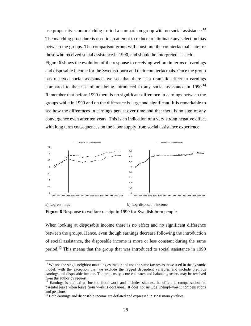
Figure 6 shows the evolution of the response to receiving welfare in terms of earnings

and disposable income for the Swedish-born and their counterfactuals. Once the group

has received social assistance, we see that there is a dramatic effect in earnings

compared to the case of not being introduced to any social assistance in 1990.14

Remember that before 1990 there is no significant difference in earnings between the

groups while in 1990 and on the difference is large and significant. It is remarkable to

see how the differences in earnings persist over time and that there is no sign of any

convergence even after ten years. This is an indication of a very strong negative effect

with long term consequences on the labor supply from social assistance experience.

4

4,5

5

5,5

6

6,5

7

7,5

1987 1988 1989 1990 1991 1992 1993 1994 1995 1996 1997 1998 1999 2000 2001

Welfare Comparison

4

4,4

4,8

5,2

5,6

6

6,4

6,8

7,2

1987 1988 1989 1990 1991 1992 1993 1994 1995 1996 1997 1998 1999 2000 2001

Welfare Comparison

a) Log-earnings b) Log-disposable income Figure 6 Response to welfare receipt in 1990 for Swedish-born people

When looking at disposable income there is no effect and no significant difference

between the groups. Hence, even though earnings decrease following the introduction

of social assistance, the disposable income is more or less constant during the same

period.15 This means that the group that was introduced to social assistance in 1990

13 We use the single neighbor matching estimator and use the same factors as those used in the dynamic model, with the exception that we exclude the lagged dependent variables and include previous earnings and disposable income. The propensity score estimates and balancing scores may be received from the author by request. 14 Earnings is defined as income from work and includes sickness benefits and compensation for parental leave when leave from work is occasional. It does not include unemployment compensations and pensions. 15 Both earnings and disposable income are deflated and expressed in 1990 money values.

29

continued to live on transfers from the welfare system for many years thereafter,

while the comparison group with significantly higher earnings (between 30 and 40

percent higher) lived on their own earnings to a higher degree.

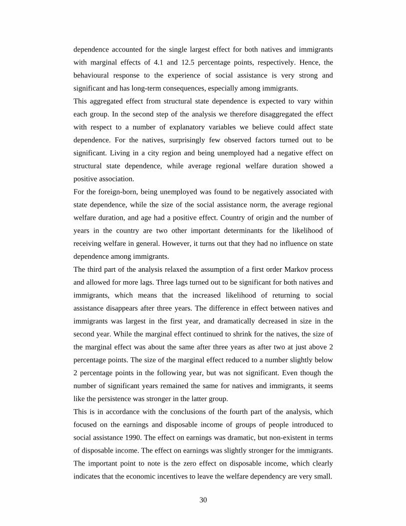
For the foreign-born the situation is comparable. Figure 7 shows their response to

social assistance in 1990, and we can see that it has a strong negative effect on

earnings but no effect on disposable income. For the foreign-born, the disposable

income is actually significantly higher in the following year (1991) for those who

received social assistance. However, this initial effect is only temporary and vanishes

in the following years. Overall, the behavior is about the same for the Swedish- and

the foreign-born welfare recipients.

4

4,5

5

5,5

6

6,5

7

7,5

1987 1988 1989 1990 1991 1992 1993 1994 1995 1996 1997 1998 1999 2000 2001

Welfare No Welfare

4

4,5

5

5,5

6

6,5

7

7,5

1987 1988 1989 1990 1991 1992 1993 1994 1995 1996 1997 1998 1999 2000 2001

Welfare No Welfare

a) Log-earnings b) Log-disposable income

Figure 7 Response to receiving welfare in 1990 for foreign-born people

6 Summary and Conclusions We estimate the size and the shape of structural state dependence in welfare

participation in terms of social assistance for natives and immigrants in Sweden. The

effects were estimated using a dynamic discrete choice model controlling for the

initial condition and unobserved heterogeneity. Four parts of the structural state

dependence were analysed.

The first part focused on the estimated size of the structural state dependence within

the framework of a first order Markov process as an aggregated measure. We found

that the effect is three times as large for immigrants as it is for natives. Furthermore,

among the explanatory variables included in the specification, structural state

30

dependence accounted for the single largest effect for both natives and immigrants

with marginal effects of 4.1 and 12.5 percentage points, respectively. Hence, the

behavioural response to the experience of social assistance is very strong and

significant and has long-term consequences, especially among immigrants.

This aggregated effect from structural state dependence is expected to vary within

each group. In the second step of the analysis we therefore disaggregated the effect

with respect to a number of explanatory variables we believe could affect state

dependence. For the natives, surprisingly few observed factors turned out to be

significant. Living in a city region and being unemployed had a negative effect on

structural state dependence, while average regional welfare duration showed a

positive association.

For the foreign-born, being unemployed was found to be negatively associated with

state dependence, while the size of the social assistance norm, the average regional

welfare duration, and age had a positive effect. Country of origin and the number of

years in the country are two other important determinants for the likelihood of

receiving welfare in general. However, it turns out that they had no influence on state

dependence among immigrants.

The third part of the analysis relaxed the assumption of a first order Markov process

and allowed for more lags. Three lags turned out to be significant for both natives and

immigrants, which means that the increased likelihood of returning to social

assistance disappears after three years. The difference in effect between natives and

immigrants was largest in the first year, and dramatically decreased in size in the

second year. While the marginal effect continued to shrink for the natives, the size of

the marginal effect was about the same after three years as after two at just above 2

percentage points. The size of the marginal effect reduced to a number slightly below

2 percentage points in the following year, but was not significant. Even though the

number of significant years remained the same for natives and immigrants, it seems

like the persistence was stronger in the latter group.

This is in accordance with the conclusions of the fourth part of the analysis, which

focused on the earnings and disposable income of groups of people introduced to

social assistance 1990. The effect on earnings was dramatic, but non-existent in terms

of disposable income. The effect on earnings was slightly stronger for the immigrants.

The important point to note is the zero effect on disposable income, which clearly

indicates that the economic incentives to leave the welfare dependency are very small.

31

References Adema, W., (2006), “Social Assistance Policy Development and the Provision of a

Decent Level of Income in Selected OECD Countries”, OECD social, employment

and migration working papers no. 38.

Budgetpropositionen (2005), “Avstämning av målet om en halvering av antalet

socialbidragsberoende mellan åren 1999-2004”, Proposition 2004/05:1 Bilaga 3.

Börsch-Supan, A., V. A. Hajivassiliou (1993), “Smooth unbiased multivariate

probability simulators for maximum likelihood estimation of limited dependent

variables”, Journal of Econometrics 58, 347-368.

Danziger, S., R. Haveman, and R. Plotnick (1981), “How Income Transfers Affect

Work, Savings, and the Income Distribution: A Critical Review”, Journal of

Economic Literature, 19, pp. 975-1028.

Gouriéroux, C., and A. Monfort (1993), “Simulation-biased inference: a survey with

special reference to panel data models”, Journal of Econometrics 59, 5-33.

Hajivassiliou, V., and P. Ruud (1994), “Classical estimation methods for LDV models

using Simulation”, in Engle, R.F., McFadden, D.L. (Eds.), Handbook of

Econometrics, Vol. 4, North-Holland, Amsterdam (Chapter 40).

Hajivassiliou, V., D. McFadden, and P. Ruud (1996), “Simulation of Multivariate

Normal Rectangle Probabilities and their Derivaties, Theoretical and

Computational Results”, Journal of Econometrics 72, 85-134.

Hansen, J., and M. Lofstrom (2003), “Immigrant Assimilation and Welfare

Participaiton: Do Immigrants Assimilate Into or Out of Welfare”, Journal of

Human Resources 38(1): 74-98.

Hansen, J., and M. Lofstrom (2006), “Immigrant-Native Differences in Welfare

Participation: The Role of Entry and Exit Rates”, IZA Discussion Paper No. 2261.

Hansen, J., M. Lofstrom, and X. Zhang (2006), ”State Dependence in Canadian

Welfare Participation”, IZA Discussion Paper No. 2266.

Heckman, J. (1981a), “Statistical Models for Discrete Panel Data”, in Structural

Analysis of Discrete Data with Econometric Applications, edited by C.F. Manski

and D. McFadden, pp. 114-178. Cambridge, MA: MIT Press.

Heckman, J. (1981b), “The Inicidental Parameters Problem and the Problem of Initial

Conditions in Estimating a Discrete Time –Discrete Data Stochastic Process”, in

Structural Analysis of Discrete Data with Econometric Applications, edited by C.F.

Manski and D. McFadden, pp. 179-195. Cambridge, MA: MIT Press.

32

Heckman, J. (1981c), “Heterogeneity and State Dependence”, in Studies in Labor

Markets, edited by S. Rosen, pp. 91-139, University of Chicago Press.

Keane, M. (1993), “Simulation estimation for panel data with limited dependent

variables”, in Maddala, G.S., Rao, C.R., Vinod, H.D. (Eds.), Handbook of

Statistics, Vol. 11, North-Holland, Amsterdam (Chapter 20).

Moffitt, R. (1992), “Incentive Effects of the U.S. Welfare System: A Review”,

Journal of Economic Literature, 30, pp. 1-61.

McFadden, D. (1973), “Analysis of Qualitative Choice Behaviour”, in Zarembka, ed.,

Frontiers in Econometrics.

Train, K. (2003), “Discrete Choice Methods with Simulation”, Cambridge University

Press.

Wooldridge, J. M., (2005), “Simple Solutions to the Initial Conditions Problem in

Dynamic, Nonlinear Panel Data Models with Unobserved Heterogeneity”, Journal

of Applied Econometrics, 20: 39-54.

Åslund, O. and P. Fredriksson (2005), “Ethnic enclaves and welfare cultures – quasis

experimental evidence”, IFAU working paper 2005:8

33

Appendix Table A1 Estimated intertemporal covariance matrix for Swedish-born Time T=1 t=2 t=3 t=4 t=5 t=6 t=7 t=8 t=9 t=10 t=1 1.0 0.418 0.479 0.466 0.446 0.493 0.411 0.446 0.351 0.399 t=2 1.0 0.409 0.465 0.456 0.452 0.438 0.383 0.397 0.369 t=3 1.0 0.414 0.497 0.523 0.476 0.410 0.412 0.385 t=4 1.0 0.457 0.455 0.527 0.511 0.489 0.452 t=5 1.0 0.476 0.494 0.459 0.510 0.381 t=6 1.0 0.503 0.529 0.525 0.486 t=7 1.0 0.443 0.512 0.459 t=8 1.0 0.456 0.515 t=9 1.0 0.530 t=10 1.0 Note: All parameters are significant at the 1% level Table A2 Estimated intertemporal covariance matrix for foreign-born Time t=1 t=2 t=3 t=4 t=5 t=6 t=7 t=8 t=9 T=10 t=1 1.0 0.402 0.437 0.396 0.425 0.405 0.383 0.345 0.349 0.273 t=2 1.0 0.361 0.425 0.441 0.442 0.410 0.351 0.385 0.296 t=3 1.0 0.318 0.454 0.445 0.395 0.372 0.374 0.297 t=4 1.0 0.403 0.349 0.476 0.413 0.452 0.325 t=5 1.0 0.402 0.486 0.457 0.518 0.374 t=6 1.0 0.398 0.518 0.471 0.369 t=7 1.0 0.461 0.555 0.434 t=8 1.0 0.473 0.413 t=9 1.0 0.355 t=10 1.0 Note: All parameters are significant at the 1% level