“The More Divergent, the Better?:

Lessons on Trilemma Policies and Crises for Asia”

Joshua Aizenman*

University of Southern California and NBER

Hiro Ito**

Portland State University

April 2014

Abstract

This paper investigates the potential impacts of the degree of divergence in open macroeconomic policies

in the context of the trilemma hypothesis. Using an index that measures the extent of policy divergence

among the three trilemma policy choices, namely monetary independence, exchange rate stability, and

financial openness, we find that emerging market countries have adopted trilemma policy combinations

with the smallest degree of policy divergence in the last fifteen years. We then investigate whether and to

what extent the degree of open macro policy convergence affects the probability of a crisis and find that a

developing or emerging market country with a higher degree of policy divergence is more likely to

experience a currency or debt crisis. We also compare the development of trilemma policies around the

crisis period for the groups of Latin American crisis countries in the 1980s and the Asian crisis countries

in the 1990s. We find that Latin American crisis countries tended to close their capital accounts in the

aftermath of a crisis while that is not the case for the Asian crisis countries. The Asian crisis countries

tended to reduce the degree of policy divergence in the aftermath of the crisis, which possibly mean that

they decided to adopt open macro policies that are less prone for a crisis.

JEL Classification Nos.: F31, F36, F41, O24

Keywords: Impossible trinity; international reserves; financial liberalization; financial crisis; exchange

rate regime.

* Aizenman: Economics and School of International Relations, University of Southern California, University Park,

Los Angeles, CA 90089-0043. Phone: +1-213-740-4066. Email: aizenman@usc.edu.

** Ito (corresponding author): Department of Economics, Portland State University, 1721 SW Broadway, Portland,

OR 97201. Tel/Fax: +1-503-725-3930/3945. Email: ito@pdx.edu

1

1. Introduction

Managing policies in an economic turbulence is never an easy task, especially when the

world economy is highly integrated and markets are intertwined with each other. History is full

of episodes where a certain international monetary system or regime ends with an abrupt end as

we have witnessed in the collapse of the Bretton Woods system in the early 1970s or in the

financial crises many emerging market economies experienced in the 1980s and 1990s. These

abrupt ends of regimes often involve crises or some sort of financial turbulence. No matter what

forms of international monetary systems or regimes they decide to replace the old ones with,

however, countries always end up adopting a combination of three policy goals: monetary

independence, exchange rate stability, and financial openness, with different degrees of

attainment in each. That is, a powerful hypothesis called the “impossible trinity,” or the

“trilemma” dictates open macro policy management. Countries may simultaneously either

choose any two, but not all, of the three policy goals to the full extent, or adopt a combination of

intermediate degrees of all or two of the three policy goals.

Theory and empirical evidence also tell us that each one of the three trilemma policy

choices can be a double-edged sword as recognized by a significant amount of recent literature.1

To make the matter more complicated, the effect of each policy choice can differ depending on

what the other policy choice it is paired with. For example, exchange rate stability can be more

destabilizing when it is paired with financial openness while it can be stabilizing if paired with

greater monetary autonomy.

Furthermore, countries rarely face the stark polarized binary choices as often envisioned

by policy makers and researchers. In the famous trilemma triangle well-used in textbooks as we

have in Figure 1, each of the three sides represents the full implementation of each of the three

policy goals. We can locate the Euro system or the gold standard at the corner that represents the

full attainment of financial openness and exchange rate stability while the Bretton Woods system

can be placed at the corner of full exchange rate stability and full monetary independence. When

a country adopts a policy combination of intermediate levels for all the three policy choices, such

a policy combination would be located somewhere inside the trilemma triangle. The bottom line

1 As for monetary independence, refer to Obstfeld, et al. (2005), Shambaugh (2004), and Frankel et al. (2004). On

the impact of the exchange rate regime, refer to Ghosh et al. (1997), Levy-Yeyati and Sturzenegger (2003), and

Eichengreen and Leblang (2003). The empirical literature on the effect of financial liberalization is surveyed by

Henry (2006), Kose et al. (2006), Prasad et al. (2003), and Prasad and Rajan (2008).

2

is, as Mundell (1963) argued, that that the extent of achievement in the three choices must be

linearly related to each other.2

Obviously, different combinations of the three policies must have different

macroeconomic effects. Now the question is, how can the location of a country’s policy

combination in the trilemma triangle affect its macroeconomic performance, especially in terms

of avoiding traumatic economic turbulence such as financial crises?

Against this backdrop, we first construct a metric that measures the degree of divergence

among the three trilemma policies while incorporating its relative position to the global trend.

With this index, we then evaluate the patterns of divergence of trilemma policy combinations in

the last four decades. In Section 3, we implement a series of empirical exercises to examine the

impact of the degree of trilemma policy divergence on macroeconomic performance, namely the

probability of the onset of a currency, banking, and debt crisis. In the end of this section, we also

compare the degree of policy divergence and trilemma policy arrangements between the Latin

American crisis countries in the 1980s and the Asian crisis countries in the 1990s and identify

commonalties and differences between these crisis periods. In Section 4, we conclude the main

findings of the paper.

2. Divergence of the Trilemma Policy Choices

2.1 Why Does the Extent of Policy Divergence Matter?

While there are only three kinds of polarized policy combinations among the three

trilemma policies, i.e., the three vertexes in the triangle in Figure 1, once intermediate levels for

each policy are allowed, there can exist an infinite number of open macro policy combinations.

Until recently, researchers have tended to focus on debating the merits and demerits of polarized

monetary regimes. Fischer (2001) argued the unstable nature of intermediate exchange rate

regimes, pointing out that such regimes are more prone to experience a crisis in a financially

globalized world. Frankel (1999), while admitting that regimes with “corner solutions” can be

simple and transparent in showing government commitment to maintaining a regime, argued that

avoiding intermediate regimes is not always the best solution for countries, especially developing

2 In other words, if there are measures representing the levels of attainment in the three policy choices, such

measures must add up to a constant, which has been empirically proved by Aizenman, et al. (2012) and Ito and

Kawai (2012).

3

ones. Willett (2003) argued that the issue is not so much about whether polarized or intermediate

regimes are more or less stable. Rather, he argues that the issue of whether macroeconomic

conditions of an economy are consistent with its monetary regime is more important. The crises

that occurred among emerging market countries in the 1980s and 1990s, and the Global

Financial Crisis of 2008-09 to a similar extent, have raised questions about the global trend of

financial liberalization, leading researchers to debate the merits and demerits of greater financial

openness.

Despite the debate, regimes with corner solutions are more of a rarity. In other words,

most countries often operate “somewhere inside the triangle.” For example, some countries

implement partial financial integration while trying to retain control over exchange rate

movement as well as monetary policy autonomy. This sort of clustering of the three policies

inside the trilemma triangle, or the “middle-ground convergence,” has been a characteristic of

emerging market countries (EMG) in recent decades as Aizenman, Chinn, and Ito (2012) have

shown. Aizenman, et al. have also found such middle-ground convergence has been more

evident among Asian EMGs in recent years.

By adopting such converged policy combinations, these countries may have been trying

to dampen the negative effects that may arise from adopting polarized policy regimes.

Interestingly, the period when EMG’s middle convergence started becoming more evident

coincides with the time when some of these economies began accumulating sizable international

reserves (IR) as if they have been trying to buffer the trade-off arising from the trilemma, again a

more evident trend among Asian EMGs.3

A natural question that arises is how the location within the trilemma triangle can affect

macroeconomic performances, especially when we focus on the risk of experiencing a financial

crisis, which this paper focuses on. Before exploring this question, however, we want to raise

one more important issue. That is, even if certain open macro policy combinations were found to

affect the likelihood of a country experiencing a crisis, such correlations may not be merely a

function of the country’s own macroeconomic policies.

A country’s open macro policies need to be evaluated in a greater context, compared with

policies adopted by other countries. For example, a fixed exchange rate regime must have

3 Aizenman, et al. (2010) empirically show that pursuing greater exchange stability can be increasing output

volatility for developing economies, but that that can be mitigated by holding a greater amount of international

reserves than the threshold of about 20% of GDP.

4

different effects on the economy depending on whether or not most of other countries also adopt

fixed exchange rate regimes as they did during the Bretton Woods period. As another example,

the consequence of liberalizing financial markets should also differ between the 1960s when

most of the countries also had closed financial markets and recent years when many countries

have been moving toward the direction of full financial liberalization.

When we think about the history of international monetary systems, anecdotally,

countries seem to have tended to adopt monetary regimes prevalent in other countries, making

the types of monetary regimes across countries correlated with each other. Such correlated

behavior can be sometimes global as was in the case of the Gold Standard in the pre-WWII era

or the Bretton Woods system, other times regional such as the Euro system, or clustered around

similar income levels such as the middle-ground convergence observed among emerging market

economies in recent years. When many countries tend to adopt similar monetary regimes, such a

herding behavior would create externality, lowering the cost of a country following such a global

or regional trend, or the “mean behavior.” Conversely, herding behavior in arranging monetary

regimes could also raise the opportunity cost of deviating from it, unless the country that deviates

from the “mean behavior” is well-equipped with healthy fundamentals or solid institutions

including well-functioning financial markets. In this sense, the pursuit of forming a monetary

union by some European countries, we could argue, can be sustainable only if they are equipped

with appropriate levels of institutional development and good fundamentals.4 Hence, again, it is

important to evaluate the combinations of open macro policies in a global context or in

comparison to other countries.

In this paper, we will particularly focus on the impact of a triad policy combination on

the likelihood of financial crisis. By financial crisis, we mean three kinds of financial crises,

namely currency, banking, and debt crisis. While it may not be difficult to consider the

relationship between the degrees of policy divergence and their impact on currency crisis, the

link between them and their impact on banking or debt crisis may not sound too straightforward.

However, the macroeconomic performance of banking or debt crisis, or the probability of its

occurrence can be direct functions of the triad policy coordination.

4 Furthermore, it means the current crisis situation faced by some of the Euro countries can be explained by their

weak fundamentals and institutional development.

5

As for the banking crisis, the recent European experience makes it clear that a choice of a

monetary regime can affect the likelihood of experiencing a banking crisis. In the case of the

Euro crisis, participating in the monetary union had made it easier for certain countries such as

Ireland, Spain, and Cyprus to experience a surge in capital flows in an unsustainable fashion.

Such capital influx ended up sowing seeds of the ongoing banking and debt crisis in these

countries. The situation could have been different if these countries had not participated in the

fixed exchange rate arrangement because it rids countries with highly open financial markets of

monetary independence.

The debt crisis in emerging market economies in the 1980s and 1990s and that in

Southern Europe such as Greece can also be explained similarly in the context of the trilemma.

For emerging market economies, particularly, the predominant global trend for financial

liberalization had made the trilemma into the dilemma between pursuing greater monetary

autonomy (with more flexible exchange rates) and greater exchange rate stability (with less

monetary autonomy). Facing the “original sin” (Eichengreen and Hausman, 1999), many

emerging market economies had chosen the path of greater exchange rate stability while the

inevitably weaker monetary independence made these economies more vulnerable to external

shocks.

Thus, not just for currency crisis, but also for banking and debt crisis, how the three

trilemma policies are coordinated by individual countries and where they stand in the global

context can be an important factor.

2.2 Measure of Policy Divergence and Its Patterns

To see how much convergence or divergence is taking place among the three trilemma

policy choices and evaluate it in a global context, we construct the “measure of divergence” in

the triad policies. For that, we use the “trilemma indexes” introduced by Aizenman, Chinn, and

Ito (2010, 2012).

The trilemma indexes measure the degree of achievement in each of the three policy

choices for more than 170 economies for 1970 through 2010.5 The monetary independence index

(MI) is based on the correlation of a country’s interest rates with the base country’s interest rate.

The index for exchange rate stability (ERS) is an invert of exchange rate volatility, i.e., standard

5 The indexes are available at http://web.pdx.edu/~ito/trilemma_indexes.htm.

6

deviations of the monthly rate of depreciation, using the exchange rate between the home and

base economies. The degree of financial integration is measured with the Chinn-Ito (2006, 2008)

capital controls index (KAOPEN). 6

Using these indexes, we define the “measure of policy divergence” as below:

√( ) ( ) ( ) (1)

where

for X = MI, ERS, and KAOPEN, and is cross-country average of X in year

t.7,8

Appendix 1 list all the countries for which d is available.

Long-run Trends

Figure 2 illustrates the average of dit for different subgroups of countries based on income

levels.9 We can make several interesting observations based on this figure. For the last two

decades, advanced economies tend to have combinations of distinctive policies. Not surprisingly,

the Euro country group has the highest degree of policy divergence among the country groups,

followed by the group of non-Euro advanced economies. Higher income countries may be able

to afford to have divergent policy combinations.

The group of emerging market economies has had the lowest degree of policy

convergence in the last two decades. Since the beginning of the 1980s, developing economies,

whether or not with emerging markets, have had relatively stable movement in the degree of

policy convergence except for the mid-1990s when both subgroups of developing economies

experienced a drop in the degree of policy divergence. In the crisis years of 1982, 1997-98, and

6 Refer to Aizenman, et al. (2012) or the index’s website for the details of construction of the indexes.

7 The cross country average (

tX ) is the sample average of X including both industrialized and developing countries

for year t. 8 One could argue that if the extents of the three trilemma policy choices are linearly related as theoretically

predicted, the above formula for d does not have to contain all the three indexes – it would need only any two of the

three trilemma indexes. However, we do not assume the linearity too strictly, i.e., the linearity does not have to hold

every single year. In other words, we assume that there is some room for policy choices to deviate from the trilemma

constraint. In fact, policy makers sometimes intentionally or unintentionally challenge the constraint of the trilemma

by implementing a policy combination that is not consistent with the trilemma hypothesis. Before aborting the fixed

exchange rate arrangement for the Thai baht, Thai policy makers attempted to challenge the trilemma by pursuing

both greater monetary independence and exchange rate stability without imposing capital controls. Also, holding a

massive amount of IR may allow countries from deviating from the constraint of the trilemma in the short run. 9 Country grouping is shown in Appendix 1.

7

2008-09 – the Mexican debt crisis, the Asian financial crisis, and the global financial crisis,

interestingly, the policy convergence measure tends to rise around the times of the crises.10

We are also curious to see if there are any regional characteristics in the formation of

triad open macro policies. As we have discussed, externality can play a role in concerting policy

decision makings among neighboring countries in a region while possibly increasing the cost of

shying away from regional policy coordination. Furthermore, there can be a regional economic

integration such as in the case of East Asian supply chain network or a monetary policy

arrangement as in the case of Gulf Cooperation Council (GCC). Hence, comparison among

geographical groups of countries should shed another ray of light on the differences in the

characteristics of triad open macro policies among countries. Figure 3 illustrates the averages of

the policy dispersion measure (dit) for different regional country groups, but focusing on Latin

American and Asian economies.

We can make an interesting observation that since the last few years of the 1990s, which

coincides with the Asian Crisis period, the degrees of policy divergence have been persistently

small among all regional groups.11

This policy convergence among developing economies may

reflect the great moderation, but the convergence seems to be still in place in the last few years

of the sample that corresponds to the years of the global financial crisis. Additionally, despite its

high levels of policy divergence in the 1980s, emerging market economies in Asia have been

experiencing lowest levels of policy divergence in the last decade.12

Behavior of d around the Time of a Crisis

Let us observe the behavior of the measure of policy dispersion around the time of a

financial crisis. Figures 4-6 show the development of the cross-country average of the degree of

policy divergence (d) for different subsamples of countries over the period for currency, banking,

and debt crises, respectively, over the period from three years before the first year of the crisis

10

To see what is driving the trajectories in Figure 2, looking at the group mean of the ratios of each of the three

indexes to its cross-country mean (i.e., t

it

XX with X for monetary policy independence (MI), exchange rate stability

(ERS), and financial openness (KAOPEN)) is helpful. For that, refer to Aizenman and Ito (2012). 11

This is also true for the group of middle-eastern or North African countries (not reported). 12

Asian emerging market economies (and countries in the middle-east, though not reported) experienced high levels

of policy divergence from the beginning of the 1980s through the early 1990s. This is partly because Latin American

countries, many of which went through debt crises, retrenched financial openness around the same period, dragging

down the average and making the financial liberalization efforts by Asian emerging market countries especially

distinctive.

8

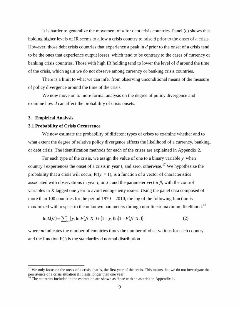
through three years after it (i.e., [t0 – 3, t0 + 3]).13

In each figure, Panel (a) shows the

development of the subsample averages of d for IDC, LDC, and EMG.14

Panel (b) shows the

development of the averages of d for the crisis countries that experienced positive output losses

as a result of a crisis (top) and those which experienced output gains (i.e., output losses < 0)

(bottom).15

Panel (c) compares the development of the d for the crisis countries with “high” IR

holding with those with “low” IR holding while “high” IR holding means that the level of IR

holding (as a share of GDP) is higher than the annual cross-country median (of all the countries

in the entire sample, including crisis and non-crisis economies) as of the year before the crisis

occurrence (t0 – 1).

We can make several interesting observations. In all three kinds of crises, there is a hump

shape of development for d around the first year of the crisis while the peak occurs at the first

year for currency crisis (t0); a year after the onset of a banking crisis (t0+1); and a year before the

onset of a debt crisis (t0–1). In the cases of currency and banking crises, if the crisis involves

output losses, the measure of policy divergence tends to stay at high levels at the first and second

years of the crisis. In the case of the crisis countries that did not experience output losses, the

countries experience a peak in d in the year before the onset of the crisis. This may imply that

these countries could avoid output losses by preemptively implementing stabilization measures

that end up raising the degree of policy divergence. 16

For the currency or banking crisis countries with low IR holding, there is a distinct rise in

d at the onset of the crisis and a distinct fall afterwards. If these countries are high IR holders, the

peak occurs in the second year of the crisis. This generalization is more apparent for the high IR

holding countries with output losses (not reported). These findings may suggest that if a country

experiences a currency or banking crisis without holding high levels of IR, the country needs to

implement policies that raise d whereas d peaks more slowly for high IR holders.

13

The methods for identifying the three types of crises are explained in Appendix 2. 14

The emerging market countries (EMGs) are defined as the countries classified as either emerging or frontier

during the period of 1980-1997 by the International Financial Corporation plus Hong Kong and Singapore. 15

Output losses are defined as the cumulative sum of the differences between actual and trend real GDP over the

four-year period (i.e., [t0, t0+3]. The trend real GDP is based on HP-filtered real GDP series over the twenty-year-

long pre-crisis period [t0 – 20, t0 – 1]. Based on whether the cumulative sum is positive or negative, a crisis is

defined to involve output losses or gains. In a sense, the existence of output losses is based on “output losses in ex

post,” not strictly as of the first year of the crisis. 16

We do not treat d as an exogenous variable. d can respond endogenously to a crisis.

9

It is harder to generalize the movement of d for debt crisis countries. Panel (c) shows that

holding higher levels of IR seems to allow a crisis country to raise d prior to the onset of a crisis.

However, those debt crisis countries that experience a peak in d prior to the onset of a crisis tend

to be the ones that experience output losses, which tend to be contrary to the cases of currency or

banking crisis countries. Those with high IR holding tend to lower the level of d around the time

of the crisis, which again we do not observe among currency or banking crisis countries.

There is a limit to what we can infer from observing unconditional means of the measure

of policy divergence around the time of the crisis.

We now move on to more formal analysis on the degree of policy divergence and

examine how d can affect the probability of crisis onsets.

3. Empirical Analysis

3.1 Probability of Crisis Occurrence

We now estimate the probability of different types of crises to examine whether and to

what extent the degree of relative policy divergence affects the likelihood of a currency, banking,

or debt crisis. The identification methods for each of the crises are explained in Appendix 2.

For each type of the crisis, we assign the value of one to a binary variable yt when

country i experiences the onset of a crisis in year t, and zero, otherwise.17

We hypothesize the

probability that a crisis will occur, Pr(yt = 1), is a function of a vector of characteristics

associated with observations in year t, or Xt, and the parameter vector β, with the control

variables in X lagged one year to avoid endogeneity issues. Using the panel data composed of

more than 100 countries for the period 1970 – 2010, the log of the following function is

maximized with respect to the unknown parameters through non-linear maximum likelihood.18

m

i tttt XFyXFyL1

'1ln1'lnln (2)

where m indicates the number of countries times the number of observations for each country

and the function F(.) is the standardized normal distribution.

17

We only focus on the onset of a crisis, that is, the first year of the crisis. This means that we do not investigate the

persistence of a crisis situation if it lasts longer than one year. 18

The countries included in the estimation are shown as those with an asterisk in Appendix 1.

10

The following variables are included in the characteristics vector Xt. The choice of the

variables is based on the past literature, except for the ones related to the degree of trilemma

policy convergence.

Variables included in the estimation:19

Relative income to the U.S. – Countries’ per capita income levels from the Penn World Table

(PWT) are normalized as a ratio to the U.S. per capita income level.

International reserves (IR) holding – IR excluding gold as a ratio to GDP .

Per capita Output growth – The growth rate of GDP per capita (in local currency).

Private credit growth – The change (first-difference) in the ratio of private credit creation to

GDP.

Net Debt inflows – The ratio of (external debt liabilities– external debt assets) to GDP. The

original data are from Lane and Milesi-Ferretti (2007 and updates).

Gross external financial exposure – The ratio of (total external assets + total external liabilities)

to GDP (from the Lane and Milesi-Ferretti dataset), included as deviations from the five-year

average of the ratios. After the global financial crisis, in addition to net capital flows or

investment positions, gross capital flows have been pointed as potential destabilizing factors.20

Real exchange rate overvaluation – It is defined as deviations from a fitted trend in the real

exchange rate. The real exchange rate is calculated using the exchange rate between country i

and its base country (in the sense of Aizenman, et al., 2011), and the CPI of the two countries.

Higher values of this variable indicate the real exchange rate value is lower, i.e., appreciated,

than its time trend.

Exchange rate stability (ERS) and Financial openness (KAOPEN) – Both are from the trilemma

indexes of Aizenman, Chinn, and Ito (2012).

19

Unless mentioned otherwise, the data for these variables are extracted mostly from publicly available datasets

such as the World Development Indicators, International Financial Statistics, and World Economic Outlook. 20

See Borio and Disyatat (2011), Obstfeld (2012a, b), Bruno and Shin (2012) for the argument on how gross

external financial exposure matters for financial and economic stability. However, it must be noted that gross

external financial exposure may also mean a higher level of ability to diversify risk, which may work as a stabilizing

fact.

11

Triad Policy Divergence Measure – The aforementioned measure of triad policy divergence dit

is included.

Standard deviations of the Triad Policy Divergence Measure – The standard deviations of the

above dit over five years from t–5 through t–1 are included to examine the impact of the stability

level of the trilemma policy combinations.

Other crises – The dummies for the other types of crises that occur either concurrently (t) or in

the previous year (t–1) are also included.

Contagion – To see the impact of other crises in the same geographical region, we also include

a variable that represents the effect of regional contagion. The variable to be included is defined

as:

K

K

P

ijj

n

tij

n

ti CDContagion1

,, (3).

CDn

i,t is a crisis dummy for type n crisis (i.e., currency, banking, or debt). kj

is the

weight based on GDP in PPP for country j ( ij ) in region K. Hence, the variable Contagionn is

the weighted sum of the dummy variables for the countries in the region country i belongs to,

excluding the weighted dummy of country i itself.21

The basic assumptions are that the more

countries in the same geographical region experience crises, the more likely it is for country i to

experience a crisis, and that the contagious effect is larger for bigger economies.

We apply the above probit estimation model to the full sample that includes both

industrialized and developing countries, the sample of industrialized countries (IDC), the sample

of developing countries (LDC), and a subsample of emerging market countries (EMG). The

baseline estimation results are reported in Table 1, which reports the marginal effects of the

explanatory variables assuming that variables take mean values (except for the dummy

variables).22,23

21

The regions we consider are: West hemisphere (i.e., North and South Americans), East and Southeast Asia and the

Pacific, South Asia, Europe (including both Western, Eastern, and Central Europe), and Sub-Saharan Africa,

Middle East and North Africa. 22

The variables that are persistently insignificant and therefore dropped from the estimation include: trade openness

measured by the sum of export and import values as a ratio to GDP; the dummy for countries’ engagement in both

internal and external armed conflicts; the dummies for commodity exporters and manufacturing exporters; the

degree of fiscal procyclicality, which is measured by the correlation between HP-detrended output and government

expenditure; the dummy for the existence of the deposit insurance; volatility of the TOT income shocks; and the

dummy for hyperinflation (with the annual rate of inflation exceeding 40%).

12

3.2 Estimation Results – The Determinants of Crisis Occurrences

We make observations of the estimations mainly for the samples of developing and

emerging market economies.

Currency crisis:

Most of the explanatory variables turn out to be qualitatively consistent with the findings

in the literature (such as Kaminsky and Reinhart, 1999; Kaminsky et al., 1998; Glick and

Hutchison, 2001; and Kaminsky, 2003) though statistical significance varies by the sample group.

Countries with real appreciation (compared to its time trend) tend to experience a currency crisis,

though significantly only for the group of industrialized countries. Rapid growth in private credit

creation (as a ratio to GDP) leads to a currency crisis especially for emerging market countries.

Not surprisingly, externally indebted countries tend to experience a currency crisis. However,

despite the prevalent strong belief, IR holding does not affect the probability of the onset of a

currency crisis.

Among developing countries, a country experiencing a banking crisis concurrently or in

the previous year tends to experience a twin crisis with currency crisis; banking crisis increases

the probability of a currency crisis by 10-12 percentage points. Debt crisis, however, does not

seem to lead to a twin crisis with currency crisis.

Regional contagion is also found to affect the probability of a currency crisis. The more

countries experience either a currency or banking crisis in the same region, the more likely it is

for a country to experience a currency crisis, although debt crisis does not have such a contagion

effect.

Among the variables of our focus, interestingly, developing or emerging market countries

that pursue more divergent triad policies from the global trend (as of a year prior to the crisis) are

more likely to experience a currency crisis although the opposite impact is found for

industrialized countries while the degree of triad policy stability does not matter for any of the

subsamples. The positive impact of a greater policy divergence on the likelihood of a currency

crisis occurring among developing countries may mean that it involves some opportunity cost for

23

In the estimation for debt crisis, the estimation results for the full or IDC sample are not reported because there is

no debt crisis data for industrialized countries in our sample period (that ends in 2010).

13

these economies to adopt a combination of open macro policies that deviates from the global

trend, which may explain why many developing economies have tended in recent years to either

adopt triad policies with middle-ground convergence, or hold a massive amount of international

reserves, or both. Contrarily, for industrialized countries, a combination of diverse policies might

help countries avoid experiencing a currency crisis, though its effect is only marginally

significant. This may suggest that industrialized countries can afford to pursue a higher degree of

policy divergence with their established policy credibility.

Banking crisis:

Generally, the banking crisis estimations also yield results qualitatively consistent with

other studies on the same subject (such as Aizenman and Noy, 2012; Demirgüç-Kunt and

Detragiache, 1998); von Hagen and Ho, 2007; Joyce, 2011; and Duttagupta and Cashin, 2011),

though with varying levels of statistical significance.

Unlike in the currency crisis estimation, IR holding now matters for the onset of a

banking crisis and lowers the probability of a banking crisis occurrence among developing and

emerging market countries. Developing or emerging market countries with faster credit growth

tend to experience banking crisis, though that is not the case for industrialized countries. While

the extent of real exchange rate overvaluation does not matter, the degree of exchange rate

stability marginally increases the probability of the onset of a banking crisis for emerging market

economies. Greater external financial exposure does increase the probability of a banking crisis

for developing countries.

Banking crisis is also found to be contagious. For the groups of developing or emerging

market economies, if other economies in the same region experience a banking crisis, that could

cause a banking crisis in the home country. Also, we again have evidence for the twin crisis of

currency and banking.

Neither the degree of triad policy divergence nor the degree of instability of the triad

policies affects the probability of bank crisis occurrence for any of the subsamples. Among the

three types of financial crises, banking crisis seems to be the most weakly linked with the extent

of triad policy divergence. One possibility for the weak link is that a certain choice of a monetary

regime affects other macroeconomic conditions in a way that these conditions would have more

direct impacts on the financial system. In the estimation result for the LDC group (column (7)) in

14

Table 1, credit growth and financial exposure are positive contributors to the likelihood of an

occurrence of a banking crisis. We can suspect that triad policy divergence may possibly affect

the probability of a banking crisis occurrence but only through these two variables. Capital can

flow to markets that are distinctively different from other markets. In the literature, it has been

argued that a policy regime with high degrees of exchange rate stability and financial openness

would often make an economy more conducive to influx of capital flows, eventually

experiencing a boom and bust cycle. That tendency can be stronger if a certain market or

economy adopts a monetary regime that is more distinct from the global trend – which can be

captured by d – compared to when many others adopt a similar monetary regime (e.g., the

Bretton Woods system). In sum, the effect of triad policy divergence could be masked by

changes in macroeconomic conditions that might have a bigger impact on the likelihood of a

banking crisis.

Debt crisis:

Not surprisingly, the more indebted externally a country is, the more likely it is to

experience a debt crisis. While greater external financial exposure does not contribute to the

probability of a debt crisis, a country pursuing greater exchange rate stability tends to experience

a debt crisis. This result may suggest that countries with fixed exchange rate regimes experience

moral hazard in their debt financing; a fixed exchange rate policy may induce over-borrowing in

hard currency. It may also be possible that a country with a fixed exchange rate tends to

procrastinate its policy adjustments even when macroeconomic conditions require an adjustment

(usually devaluation) of its currency, letting the peg duration increase the political cost of

devaluation. These findings are consistent with the negative impact of IR holding on the

probability of a debt crisis occurrence.

Currency crisis in the same region could also lead to an occurrence of a debt crisis. The

significantly negative sign on the debt crisis contagion variable is somewhat puzzling. However,

that may mean that once a country in the same geographical proximity, especially an

economically larger one, experiences a debt crisis and goes through some form of rescheduling,

that may calm down the sovereignty bond market for other countries with similar income levels

in the region.

15

Again, a higher degree of triad policy divergence tends to lead to debt crisis. If a country

pursues a distinctly more divergent triad policy compared to the global trend, that may cause

stress on the economy. Possibly, investors would start suspecting the sustainability of the

country’s policy management and therefore question the future ability of repaying the debt.

Such stress may become self-fulfilling and eventually force the country to experience a debt

crisis. The instability of the triad policy combination also matters though only with marginal

significance. That also implies that unstable open macro policy management may weaken the

credibility of the country in terms of its policy management and debt sustainability, and lead

investors to attack speculatively the country’s sovereign bond markets.

Impact of IR holding

Can the impact of the degree of triad policy convergence, d, on the probability of crisis

occurrence be conditional on another factor, such as IR holding? One may expect a greater

amount of IR holding might help lessen the positive effect of d on the probability of experiencing

a crisis. If that is the case, countries with lower amounts of IR holding may be likely to

experience a crisis once they increase the levels of d, while those with higher amounts of IR

holding may not. To examine this, we re-estimate the probit model while dividing the sample

into two groups: one composed of country-year’s with IR holding higher than the annual median

(as of t-1) and the other of IR holding lower than the median.

We report the estimation results of IR holding, d, its volatility, and private credit growth

for both high and low IR regimes in Table 2.24

In the table, the coefficient on d is significant

among the low IR holders for the debt crisis estimation while it is no longer significant for the

high IR holders that experience debt crisis. These findings are consistent with our prior. However,

for the currency crisis estimation, the estimate on d is significant for the high IR holding regime

for both developing and emerging market groups. This result is somewhat counterintuitive. To

interpret this ostensibly counterintuitive result, we could expect that countries with high IR

holdings may experience other macroeconomic symptoms that may create an environment where

higher policy dispersion can lead to an occurrence of a crisis. Interestingly, private credit growth

is a positive contributor to the likelihood of a crisis occurrence among high IR-holding

24

The estimates of the other variables than those reported in Table 2 are omitted from presentation to conserve space.

They are available from the authors upon request.

16

developing or emerging market countries in either the currency or banking crisis estimation,

while it is not the case for any type of crisis among the low IR holders, or for debt crisis

irrespective of the IR regime type. These results suggest that in the high IR regime, IR holdings

may tend to induce higher credit growth, which would in return likely lead to a currency or

banking crisis. In such an environment, pursuing a higher degree of policy divergence is riskier

and tends to lead to a currency crisis. The distinct roles of private credit growth in currency and

debt crisis may explain the twists in the results for the currency and debt crisis estimations.

Furthermore, the finding that, for the low IR regime, the estimate on the IR holding

variable is persistently negative among all the samples and significant among most of them,

suggests that the effect of IR holding can be nonlinear. In other words, the effect of an

incremental change in the level of IR holding may be larger for lower IR holders than for higher

IR holders.

3.3 Discussions – What Do the Estimation Results Tell Us about the Experiences in Latin

America and Asia?

Now, we examine what we can learn from the estimation results as well as the actual

crisis experiences. For that, we take a look at the two big crisis episodes in the 1980s and 1990s,

namely the Latin American debt crisis in the early 1980s and the Asian crisis of 1997-1998.

Figure 7 shows the averages of d around the crisis period for the groups of Latin

American and Asian countries.25

The year of a crisis onset (year 0 in the graph) differs between

the sample groups, and also among the countries within the Latin American group. For each of

the Latin American countries, “Year 0” indicates the year when the crisis is the most severe

among the years: 1981, 1982, or 1983.26

For the Asian countries, “Year 0” is always 1997. The

figure illustrates the sample average of d over the period from five years before (t0 – 5) through

five years after the crisis year (t0 + 5).

From the figure, we can see that Latin American countries tend to have higher d in the

period prior to the crisis compared to the Asian counterpart. Second, for this group of crisis

countries, the policy divergence variable increases over the post-crisis period. Third, for the

25

The “Latin America” crisis countries include: Argentina, Bolivia, Brazil, Chile, Columbia, Costa Rica, Ecuador,

El Salvador, Honduras, Mexico, Peru, Uruguay, and Venezuela. The “Asian” crisis countries include: Indonesia,

Korea, Malaysia, the Philippines, and Thailand. 26

The year with the “most severe crisis” is identified when one of the years 1981, 1982, and 1983 is the starting year

for different types of crises that occur in consecutive years, or the year when a twin or triple crisis occurs.

17

Asian group, d rises rapidly when the crisis breaks out, making it look more like countries are

increasing the level of policy divergence in response to the occurrence of a crisis. Fourth, unlike

the Latin American counterparts, d drops in the second year after the crisis and remains at

relatively low levels afterwards.

The fact that d remains at relatively lower levels in the post-crisis period may suggest that

Asian countries have possibly adopted policy combinations that would help reduce the likelihood

of repeating a crisis. As far as the post-crisis period is concerned, Asian crisis countries appear

more crisis-proof than Latin American countries in the 1980s.

Considering the previous finding that the positive correlation between the degree of

policy dispersion and the likelihood of a currency crisis survives even if a country holds a large

amount of IR (Table 2), Asian crisis countries’ efforts to maintain lower levels of policy

dispersion from the global trend do matter, and may have helped these economies to stay less

crisis-prone in the post-Asian crisis years.

In Figure 8, we can observe the development of the measure of policy divergence for

individual crisis countries: Argentina, Brazil, Chile, Columbia, and Mexico in panel (a) and

Indonesia Korea, Malaysia, Philippines, and Thailand in panel (b). The individual countries’

experiences provide interesting information that may be masked by the average behaviors

illustrated in Figure 7. First, the movement of d is more diverse among Latin American crisis

countries than Asian counterparts. Second, the degree of diversity is especially greater before the

crisis-breakout year for Latin American countries, and it diminishes as years go by in the post-

crisis period. Among Asian countries, except Indonesia, the level and the movement of d tends to

be more homogenous, which may suggest the extent of policy coordination is greater in the

Asian region. Third, among the economies in this region, the peak of d tends to be clustered

around the first year of a crisis occurrence, preceded by lower levels of d and followed again by

lower d, but moderately higher than in the pre-crisis years. Such a generalization is not

applicable to Latin American economies. Last, as we observed in Figure 7, Asian crisis

economies tend to implement policy combinations in a way that homogenously leads to

declining d over post-crisis years, which is not observable among Latin American crisis

economies.

Figure 9 takes a closer look at the policy combinations of the economies from the two

regions. It illustrates the development of the sample averages of mean deviations for each of the

18

three trilemma policy indexes, i.e., : ⁄ ,

⁄ , and ⁄ for

both groups. This figure allows us to see how the movement in the three trilemma indexes is

driving the results we saw in Figures 7 and 8.

According to this figure, while both Latin American and Asian countries experienced the

crisis with relatively high levels of financial openness, Latin American countries significantly

reduced the level of financial openness in the post-crisis period. The mean deviations of the

financial openness index show (not reported) that countries such as Bolivia, Chile, Mexico, and

Argentina reduced the degree of financial openness (with respect to the global trend)

significantly. Asian crisis countries also did reduce the level of financial openness (such as

Malaysia and Indonesia), but only by a lesser degree than Latin American counterparts.

Considering that Latin American economies did not have high domestic savings in the pre-debt

crisis years while Asian economies did have by the 1990s, the Latin American economies could

have been more vulnerable to external shocks than Asian counterparts. That may explain the

difference in the response to financial openness in the post-crisis years.

Both groups experienced a fall in the level of exchange rate stability, but the extent of the

fall is greater for Asian countries on average. Part of the smaller decline in the extent of

exchange rate stability for Latin American crisis countries is due to relatively dispersed timings

of aborting fixed exchange regimes. While Asian crisis countries aborted their fixed exchange

rate arrangements as soon as they experienced a currency crisis, the Latin American reactions to

a crisis occurrence in terms of exchange rate stability differ widely across the countries. Some

countries allowed exchange rate flexibility immediately after experiencing a crisis while others

tried to maintain exchange rate stability. Furthermore, all the Asian countries, except for

Malaysia, maintained exchange rate flexibility in the post-crisis five year period while such a

homogeneity is not observed among Latin American counterparts.

Asian crisis countries have maintained stable levels of monetary independence

throughout the pre- and post-crisis period though it did lose some degree of monetary

independence at the time of crisis occurrence. As was the case with exchange rate stability, the

movement of the monetary independence indexes for the Asian countries is much more

homogenous than for the Latin American countries, again suggesting more policy coordination

among these economies. On average, Latin American countries moderately increased the level of

19

monetary independence a year before the crisis year through three years after the occurrence of a

crisis.

Due to the way the variable d is constructed, if any of the three indexes is far from the

value of one, that would tend to raise the value of d. Given that, we can observe that Asian crisis

countries have maintained relatively low levels of d because they tend to be “conformists” to the

world trend in terms of monetary independence and financial openness. Despite the oft-discussed

anecdote, Asian crisis countries have maintained relatively low levels of exchange rate stability,

that allowed these countries to have more conformist trilemma policy combinations.

Latin American countries in the post-crisis period in the 1980s tended to have

combinations of three distinct policies. They retained high (i.e., more-than-average) levels of

monetary independence with lower exchange rate stability. Most importantly, these countries

decided to seclude themselves from international financial markets. Such policy response,

ironically, may have left the economies exposed to a crisis-prone state – though there are surely

other factors that contributed to keeping the economies prone for crisis.

Given these findings, what makes Asia different the most is that, despite the turbulent

experience of the Asian crisis, Asian countries have decided not to move away from the global

trend of financial liberalization. As Aizenman, et al. (2011) show, these economies seem to have

decided to learn how to surf on the waves of financial globalization rather than run away from

them.

4. Conclusion

We have examined the impact of open macro policies on the economies from the

perspective of the powerful hypothesis of the “trilemma” – a country may not simultaneously

pursue the full extent of achievement in all of the three policy goals of monetary independence,

exchange rate stability, and financial openness. In this paper, we shed light on a new aspect of

the trilemma by focusing on the degree of policy divergence, i.e., how far a country’s trilemma

policy combination differs from the world trend.

We find a wider variation in the degree of policy divergence across countries among

different income levels and also geographical groups. Industrialized countries, most notably the

Euro countries, tend to adopt more diverse trilemma policy combinations since the early 1990s.

20

In the last 15 years or so, emerging market countries have adopted trilemma policy combinations

with the smallest degree of policy divergence. Given that this group of countries has achieved

relatively stable output performance, lower levels of policy divergence may have been one of the

keys to it.

To investigate that, we formally tested the effect of the degree of policy divergence on

the probability of crisis occurrences.

We have found that a developing or emerging market country with a higher degree of

policy divergence is more likely to experience currency or debt crisis. For industrialized

countries, a higher degree of policy divergence tends to reduce the probability of currency or

banking crisis, however. We also found that by holding large volumes of IR, developing

countries could avoid facing the correlation between wider policy divergence and a higher level

of likelihood of experiencing a debt crisis, though high IR holders, interestingly, would also face

a positive correlation between wider policy divergence and the likelihood of experiencing a

currency crisis. Our results also suggest a non-linearity in the effect of IR holding; i.e., the effect

of an incremental change in the level of IR holding may be larger for lower IR holders

When we examined the development of trilemma policies around the crisis period for the

groups of Latin American crisis countries in the 1980s and the Asian crisis countries in the 1990s,

we found that these two groups of countries have gone through distinctly different policy

development around the time of the crisis. The biggest difference between the two groups of

crisis countries is that Latin American crisis countries tended to close their capital accounts in

the aftermath of a crisis while that is not the case among the Asian crisis countries. Furthermore,

the Asian crisis countries tend to reduce the degree of policy divergence in the aftermath of the

crisis, which possibly means that they decided to adopt open macro policies that are less prone

for a crisis. That decision has been paired with a strong incentive to hold a great amount of

international reserves. By observing how crisis-prone conditions can be perennial for emerging

market economies as it happened to Latin American countries, Asian economies, including those

which did not experience a crisis like China, seem to have decided to become a cautious

implementer of open macro policies. In the highly integrated world economy, this decision is no

surprise to anyone.

21

References

Abiad, Abdul, Ravi Balakrishnan, Petya Koeva Brooks, Daniel Leigh, and Irina Tytell. 2009.

“What’s the Damage? Medium-term Output Dynamics After Banking Crises,” IMF

Working Papers 09/245, Washington, D.C.: International Monetary Fund.

Angkinand Prabha, Apanard P. 2008. “Output Loss and Recovery from Banking and Currency

Crises: Estimation Issues,” Mimeo, available at SSRN: http://ssrn.com/abstract=1320730.

Aizenman, Joshua, and Hiro Ito. 2012. “Trilemma Policy Convergence Patterns and Output

Volatility.” North American Journal of Economics and Finance, Volume 23, Issue 3,

December 2012, Pages 269–285 (December 2012).

Aizenman, Joshua, Menzie D. Chinn, and Hiro Ito. 2012. “The ‘Impossible Trinity’ Hypothesis

in an Era of Global Imbalances: Measurement and Testing.” University of Wisconsin-

Madison Working Paper. Forthcoming in Review of International Economics.

Aizenman, Joshua, Menzie D. Chinn, and Hiro Ito. 2011. “Surfing the Waves of Globalization:

Asia and Financial Globalization in the Context of the Trilemma,” Journal of the

Japanese and International Economies, vol. 25(3), p. 290 – 320 (September).

Aizenman, Joshua, Menzie D. Chinn and Hiro Ito. 2010. “The Emerging Global Financial

Architecture: Tracing and Evaluating the New Patterns of the Trilemma's Configurations,”

Journal of International Money and Finance, Vol. 29, No. 4, p. 615-641.

Aziz, Jahangir, Francesco Caramazza and Ranil Salgado. 2000. “Currency Crisis: In Search of

Common Elements,” IMF Working Paper WP/00/67 (March)

Babbel, David F. 1995. “Insuring Sovereign Debt Against Default,” World Bank Discussion

Paper Series, Washington, D.C.: World Bank.

Beim, David and Charles Calomiris. 2001. Emerging Financial Markets. New York: McGraw-

Hill/Irwin Publishers.

Borio, Claudio E. V. and Piti Disyatat. 2011. “Global Imbalances and the Financial Crisis: Link

or No Link?” BIS Working Paper No. 346 (May 1).

Bruno, Valentina and Hyun Song Shin. 2012. “Capital Flows, Cross-Border Banking and Global

Liquidity,” Princeton Working Paper.

Chinn, Menzie D. and Hiro Ito. 2008. “A New Measure of Financial Openness,” Journal of

Comparative Policy Analysis, Volume 10, Issue 3 (September), p. 309 - 322.

Chinn, Menzie D. and Hiro Ito. 2006. “What Matters for Financial Development? Capital

Controls, Institutions, and Interactions,” Journal of Development Economics, Volume 81,

Issue 1, Pages 163-192 (October).

Demirgüç-Kunt, Asli and Enrica Detragiache. 1998. “The Determinants of Banking Crises in

Developing and Developed Countries,” IMF Staff Papers 45, 81–109.

Duttagupta, Rupa and Paul Cashin. 2011. “Anatomy of banking Crises in Developing and

Emerging Market Countries,” Journal of International Money and Finance, 30(2), p.

354‐376.

Demirgüç-Kunt, Asli, Baybars Karacaovali and Luc Laeven. 2005. “Deposit Insurance around

the World: A Comprehensive Database.” World Bank Policy Research Working Paper no.

3628.Washington, DC: World Bank.

Eichengreen, Barry and Ricardo Hausmann. 1999. “Exchange Rates and Financial Fragility,” In

New Challenges for Monetary Policy. Proceedings of a symposium sponsored by the

Federal Reserve Bank of Kansas City.

22

Eichengreen, Barry and David Leblang. 2003. “Exchange Rates and Cohesion: Historical

Perspectives and Political-Economy Considerations,” Journal of Common Market Studies,

41(5): 797–822.

Eichengreen, Barry, Andrew Rose and Charles Wyplosz. 1995. “Exchange Market Mayhem: The

Antecedents and Aftermaths of Speculative Attacks”, Economic Policy, 21, pp. 249-312,

October.

Eichengreen, Barry, Andrew Rose and Charles Wyplosz. 1996. “Contagious Currency Crises:

First Tests”, Scandinavian Journal of Economics, 98(4), pp. 463−484.

Fischer, Stanley. 2001. “Exchange Rate Regimes: Is the Bipolar View Correct?” Journal of

Economic Perspectives, 15(2): 3-24.

Frankel, Jeffrey A. 1999. “No Single Currency Regime is Right for All Countries or at All

Times,” Essays in International Finance No. 215 (Princeton University Press: Princeton).

Frankel, Jeffrey A., Sergio L. Schmukler, and Luis Serven. 2004. “Global Transmission of

Interest Rates: Monetary Independence and Currency Regime,” Journal of International

Money and Finance, 2004, v23(5,Sep), 701-733.

Ghosh, Atish, Anne-Marie Gulde, Jonathan Ostry and Holger C. Wolf. 1997. “Does the Nominal

Exchange Rate Regime Matter?” NBER Working Paper No 5874.

Glick, Reuven and Michael M. Hutchison. 2001. “Banking and Currency Crises: How Common

Are Twins?” In R. Glick, R. Moreno, and M. Spiegel, eds. Financial Crises in Emerging

Markets. Cambridge, UK: Cambridge University Press, Chapter 2.

Gupta, Poonam, Deepak Mishra and Ratna Sahay. 2000. “Output Response During Currency

Crises.” Working paper, IMF.

Henry, Peter Blair 2007. “Capital Account Liberalization: Theory, Evidence, and Speculation,”

Journal of Economic Literature, vol. 45(4), p. 887-935 (December).

Ito, Hiro and Masahiro Kawai. 2012. “New Measures of the Trilemma Hypothesis and Their

Implications for Asia.” ADBI Working Paper 381 (February).

Joyce, Joseph, 2011. “Financial Globalization and Banking Crises in Emerging Markets,” Open

Economies Review, vol. 22 no. 5.

Kaminsky, Graciela L. 2003. “Varieties of Currency Crises” NBER Working Paper Series,

#10193.

Kaminsky, Graciela L. and Carmen M. Reinhart. 1999. “The Twin Crises: The Causes of

Banking and Balance-of-Payments Problems,” American Economic Review, vol. 89(3),

pages 473-500.

Kaminsky, Graciela L, Saul Lizondo, and Carmen M. Reinhart. 1998. “Leading Indicators of

Currency Crises,” International Monetary Fund Staff Papers, 45, March, 1-48.

Kaminsky, Graciela, and Sergio Schmukler. 2002, “Short-Run Pain, Long-Run Gain: The Effects

of Financial Liberalization,” World Bank Working Paper No. 2912.

Kapp, Daniel and Marco Vega. 2012. “Real Output Costs of Financial Crises: A Loss

Distribution Approach,” Papers 1201.0967, arXiv.org (May).

Kose, M. Ayhan, Eswar Prasad, Kenneth Rogoff, and Shang-Jin Wei. 2006. “Financial

Globalization: A Reappraisal.” IMF Working Paper, WP/06/189. Washington, D.C.:

International Monetary Fund.

Laeven, Luc and Fabian Valencia. 2008. “Systematic Banking Crises: A New Database,” IMF

Working Paper WP/08/224, Washington, D.C.: International Monetary Fund.

23

Laeven, Luc and Fabian Valencia. 2010. “Resolution of Banking Crises: The Good, the Bad, and

the Ugly,” IMF Working Paper No. 10/44. Washington, D.C.: International Monetary

Fund.

Laeven, Luc and Fabian Valencia. 2012. “Systematic Banking Crises: A New Database,” IMF

Working Paper WP/12/163, Washington, D.C.: International Monetary Fund.

Levy-Yeyati, Eduardo and Federico Sturzenegger. 2003. “To Float or to Fix: Evidence on the

Impact of Exchange Rate Regimes on Growth,” The American Economic Review 93(4):

1173–1193.

Mundell, Robert A. 1963. “Capital Mobility and Stabilization Policy under Fixed and Flexible

Exchange Rates,” Canadian Journal of Economic and Political Science. 29 (4). pp. 475–

85.

Obstfeld, Maurice. 2012a. “Financial Flows, Financial Crises, and Global Imbalances,” Journal

of International Money and Finance, 31, p. 469-480.

Obstfeld, Maurice. 2012b. “Does the Current Account Still Matter?”, American Economic

Review, 102(3), 1-23.

Obstfeld, Maurice, Jay. C. Shambaugh, and Alan M. Taylor. 2005. “The Trilemma in History:

Tradeoffs among Exchange Rates, Monetary Policies, and Capital Mobility." Review of

Economics and Statistics 87 (August): 423-38.

Popper Helen, Alex Mandilaras, and Graham Bird. 2011. “Trilemma Stability and International

Macroeconomic Archetypes,” manuscript, Santa Clara University.

Prasad, Eswar S. and Raghuram Rajan. 2008. “A Pragmatic Approach to Capital Account

Liberalization,” NBER Working Paper #14051. (June).

Prasad, Eswar S., Kenneth Rogoff, Shang-Jin Wei, and M. Ayan Kose. 2003. “Effects of

Financial Globalization on Developing Countries: Some Empirical Evidence,”

Occasional Paper 220. Washington, D.C.: International Monetary Fund.

Reinhart, Carmen M. and Kenneth Rogoff. 2009. This Time is Different: Eight Centuries of

Financial Folly, Princeton: Princeton University Press.

Reinhart, Carmen M. and Kenneth Rogoff. 2008. “The Forgotten History of Domestic Debt,”

NBER Working Paper #13946.

Shambaugh, Jay C. 2004. “The Effects of Fixed Exchange Rates on Monetary Policy.” Quarterly

Journal of Economics 119 (February): 301-52.

Willett, Thomas. 2003. “Fear of Floating Needn't Imply Fixed Rates: An OCA Approach to the

Operation of Stable Intermediate Currency Regimes,” Open Economies Review, Springer,

vol. 14(1), pages 71-91 (January).

World Bank. 2012. Global Development Finance – External Debt of Developing Countries.

Washington, D.C.: World Bank.

24

Appendix 1: Country List

Industrialized Countries

1 193 Australia*

2 122 Austria*

3 124 Belgium*

4 156 Canada*

5 128 Denmark*

6 172 Finland*

7 132 France*

8 134 Germany*

9 174 Greece*

10 176 Iceland*

11 178 Ireland*

12 136 Italy*

13 158 Japan*

14 181 Malta

15 138 Netherlands*

16 196 New Zealand*

17 142 Norway*

18 182 Portugal*

19 184 Spain*

20 144 Sweden*

21 146 Switzerland*

22 112 United Kingdom*

Developing Countries: (E) denotes emerging market

countries

23 914 Albania*

24 612 Algeria*

25 614 Angola*

26 311 Antigua and Barbuda

27 213 Argentina*, (E)

28 911 Armenia*

29 314 Aruba

30 912 Azerbaijan

31 313 Bahamas, The

32 419 Bahrain

33 513 Bangladesh*

34 316 Barbados

35 913 Belarus

36 339 Belize

37 638 Benin*

38 514 Bhutan

39 218 Bolivia*

40 616 Botswana, (E)

41 223 Brazil*, (E)

42 918 Bulgaria*, (E)

43 748 Burkina Faso*

44 618 Burundi*

45 662 Cote d'Ivoire*, (E)

46 522 Cambodia, (E)

47 622 Cameroon*

48 624 Cape Verde*

49 626 Central African Republic*

50 628 Chad*

51 228 Chile*, (E)

52 924 China*, (E)

53 233 Colombia*, (E)

54 632 Comoros

55 636 Congo, Dem. Rep.

56 634 Congo, Rep.

57 238 Costa Rica*

58 960 Croatia*

59 423 Cyprus

60 935 Czech Republic*, (E)

61 611 Djibouti

62 321 Dominica

63 243 Dominican Republic*

64 248 Ecuador, (E)

65 469 Egypt, Arab Rep.*, (E)

66 253 El Salvador*

67 642 Eq. Guinea*

68 939 Estonia*

69 644 Ethiopia

70 819 Fiji

71 646 Gabon

72 648 Gambia, The

73 915 Georgia*

74 652 Ghana*, (E)

75 328 Grenada

76 258 Guatemala*

77 656 Guinea

78 654 Guinea-Bissau*

79 336 Guyana*

80 263 Haiti

81 268 Honduras*

82 532 Hong Kong, China*, (E)

83 944 Hungary*, (E)

84 534 India*, (E)

85 536 Indonesia*, (E)

86 429 Iran, Islamic Rep.

87 436 Israel*, (E)

88 343 Jamaica*, (E)

89 439 Jordan*, (E)

90 916 Kazakhstan*

91 664 Kenya*, (E)

92 542 Korea, Rep.*, (E)

93 443 Kuwait*

94 917 Kyrgyz Republic*

95 544 Lao PDR

96 941 Latvia*

97 446 Lebanon

98 666 Lesotho

99 668 Liberia

100 672 Libya

101 946 Lithuania*, (E)

102 674 Madagascar*

103 676 Malawi

104 548 Malaysia*, (E)

105 556 Maldives

25

106 678 Mali*

107 682 Mauritania*

108 684 Mauritius*, (E)

109 273 Mexico*, (E)

110 868 Micronesia, Fed. Sts.

111 921 Moldova

112 948 Mongolia*

113 686 Morocco*, (E)

114 688 Mozambique*

115 518 Myanmar

116 728 Namibia

117 558 Nepal*

118 353 Netherlands Antilles

119 278 Nicaragua

120 692 Niger*

121 694 Nigeria*, (E)

122 449 Oman

123 564 Pakistan

124 283 Panama*

125 853 Papua New Guinea

126 288 Paraguay*

127 293 Peru*, (E)

128 566 Philippines*, (E)

129 964 Poland*, (E)

130 453 Qatar

131 968 Romania*

132 922 Russian Federation*, (E)

133 714 Rwanda

134 716 Sao Tome and Principe

135 862 Samoa

136 456 Saudi Arabia

137 722 Senegal*

138 718 Seychelles

139 724 Sierra Leone*

140 576 Singapore*, (E)

141 936 Slovak Republic*, (E)

142 961 Slovenia*, (E)

143 813 Solomon Islands

144 199 South Africa*, (E)

145 524 Sri Lanka*

146 361 St. Kitts and Nevis

147 362 St. Lucia

148 364 St. Vincent & the Grenadines

149 732 Sudan

150 366 Suriname

151 734 Swaziland*

152 463 Syrian Arab Republic

153 923 Tajikistan

154 738 Tanzania*

155 578 Thailand*, (E)

156 742 Togo*

157 866 Tonga

158 369 Trinidad and Tobago, (E)

159 744 Tunisia*, (E)

160 186 Turkey*, (E)

161 746 Uganda*

162 926 Ukraine

163 298 Uruguay*

164 846 Vanuatu

165 299 Venezuela, RB*, (E)

166 582 Vietnam*, (E)

167 474 Yemen, Rep.*

168 754 Zambia*

169 698 Zimbabwe*, (E)

Note: Countries with “*” are the ones included in the

regression estimations. (E) denotes “emerging market

economies.”

26

Appendix 2: Crisis Identification

Currency crisis – We identify the currency crisis based on the conventional exchange rate market

pressure (EMP) index pioneered by Eichengreen et al. (1995, 1996). The EMP index is defined

as a weighted average of monthly changes in the nominal exchange rate, the international reserve

loss in percentage, and the nominal interest rate. The nominal exchange rate is calculated against

the base country that we use to construct the trilemma indexes (see Aizenman, et al., 2008).27

The weights are inversely related to the pooled variance of changes in each component over the

sample countries. As many others do, we use two standard deviations of the EMP as the

threshold to identify a currency crisis. For the countries whose data for the EMP are not available,

we supplement the crisis dummy with the currency crisis identification by Reinhart and Rogoff

(2009). The crisis dummy is available for 1970 – 2010.

Banking crisis – It is based on the data developed by Laeven and Valencia (2008, 2010) and its

update (Laeven and Valencia, 2012). Laeven and Valencia define a systematic banking crisis if

an economy is showing “significant signs of financial distress in the banking system” (e.g.,

significant bank runs, losses in the banking system, and/or bank liquidations) and if the

government has taken “significant banking policy intervention measures in response to

significant losses in the banking system.” They consider “significant banking policy intervention

measures” have been taken if at least three out of the following six measures have been used: 1)

extensive liquidity support (5 percent of deposits and liabilities to nonresidents); 2) bank

restructuring gross costs (at least 3 percent of GDP); 3) significant bank nationalizations; 4)

significant guarantees put in place; 5) significant asset purchases (at least 5 percent of GDP); and

6) deposit freezes and/or bank holidays. See Laeven and Valencia (2008) for more details. We

also supplement the data with the Reinhart and Rogoff data. The data are available for 1970 –

2010.

27

The “base country” is defined as the country that a home country’s monetary policy is most closely linked with as

in Shambaugh (2004). The base countries are Australia, Belgium, France, Germany, India, Malaysia, South Africa,

the U.K., and the U.S. The base country can change as it has happened to Ireland, for example. Its base country was

the U.K. until the mid-1970s, and changed to Germany since Ireland joined the EMS.

27

Debt crisis – It is identified using the dataset by Reinhart and Rogoff (2009). They identify a

sovereignty default when a country fails to meet a principle or interest payment on the due date.

Or, a debt crisis is identified when “rescheduled debt is ultimately extinguished in terms less

favorable than the original obligation.” We also augment the Reinhart and Rogoff data using the

information from Babbel (1995), Beim, D. and C. Calomiris. (2001), Reinhart and Rogoff (2008),

and World Bank’s Global Development Finance (2012). The data are available for 1970 – 2010.

Twin crises – A twin crisis is identified when one type of crisis occurs while another type occurs

in the immediate previous year (t0–1), the same year (t0), or the immediate following year (t0+1).

28

Table 1: Probit Estimations on the Probabilities of Different Types of Crisis Occurrences

(1) Currency (2) Currency (3) Currency (4) Currency (5) Banking (6) Banking (7) Banking (8) Banking (9) Debt (10) Debt

Full IDC LDC EMG FULL IDC LDC EMG LDC EMG

Relative income 0.041 0.051 0.064 0.026 -0.017 0.001 0.012 0.026 -0.108 -0.023

(t-1) (0.015)*** (0.035) (0.027)** (0.040) (0.014) (0.004) (0.026) (0.037) (0.049)** (0.026)

IR holding (t-1) -0.004 -0.156 0.001 0.008 -0.093 0.003 -0.131 -0.122 -0.124 -0.079

(0.041) (0.135) (0.044) (0.075) (0.041)** (0.016) (0.047)*** (0.064)* (0.050)** (0.031)**

Per Capita -0.071 -0.243 -0.032 0.016 -0.124 -0.063 -0.063 -0.032 -0.134 -0.214

Output growth (t-1) (0.078) (0.206) (0.077) (0.161) (0.067)* (0.053) (0.069) (0.115) (0.113) (0.088)**

Private credit growth 0.015 0.056 0.035 0.190 0.097 0.002 0.209 0.150 -0.104 -0.070

(t-1) (0.067) (0.079) (0.088) (0.096)** (0.045)** (0.012) (0.070)*** (0.076)** (0.128) (0.065)

Net Debt (t-1) 0.006 -0.004 0.021 0.052 0.008 0.005 0.007 -0.002 0.046 0.006

(0.006) (0.015) (0.007)*** (0.023)** (0.006) (0.004) (0.008) (0.016) (0.015)*** (0.012)

Real Exchange 0.019 0.105 0.007 -0.004 0.005 0.010 0.003 0.011 -0.002 -0.001

Overvaluation (t-1) (0.010)* (0.041)** (0.009) (0.020) (0.013) (0.008) (0.015) (0.020) (0.014) (0.011)

Financial Exposure -0.017 -0.023 -0.002 -0.025 0.013 0.004 0.015 0.010 -0.007 -0.012

(t-1) (0.006)*** (0.011)** (0.009) (0.019) (0.004)*** (0.004) (0.006)*** (0.007) (0.016) (0.014)

ERS (t-1) -0.012 -0.025 0.006 0.001 0.009 -0.002 0.009 0.020 0.035 0.016

(0.011) (0.019) (0.012) (0.018) (0.009) (0.004) (0.011) (0.017) (0.016)** (0.012)

KAOPEN (t-1) -0.042 -0.027 -0.024 -0.023 -0.009 -0.003 -0.011 -0.015 -0.001 -0.016

(0.015)*** (0.024) (0.015) (0.021) (0.012) (0.007) (0.013) (0.018) (0.016) (0.011)

Tri. Pol. Conv (t-1) 0.001 -0.022 0.036 0.043 0.005 0.002 -0.000 0.011 0.051 0.024

(0.011) (0.014) (0.014)*** (0.019)** (0.010) (0.003) (0.013) (0.017) (0.017)*** (0.010)**

Tri-Pol. Conv., SD 0.035 -0.001 0.039 0.052 0.045 0.012 0.027 0.024 0.081 0.038

(t-5|t-1) (0.036) (0.053) (0.041) (0.057) (0.033) (0.012) (0.042) (0.056) (0.053)13% (0.025)11%

Contagion: Currency 0.143 0.078 0.135 0.117 -0.050 -0.024 -0.042 0.025 0.076 -0.019

(t or t-1) (0.030)*** (0.047)* (0.031)*** (0.066)* (0.035) (0.021) (0.036) (0.049) (0.040)* (0.045)

Contagion: Banking 0.035 -0.034 0.055 0.093 0.124 0.027 0.073 0.089 -0.022 0.007

(t or t-1) (0.025) (0.036) (0.024)** (0.034)*** (0.018)*** (0.026) (0.019)*** (0.027)*** (0.038) (0.025)

Contagion: Debt -0.015 -0.075 -0.003 0.046 0.005 0.046 -0.023 0.005 -0.234 -0.129

(t or t-1) (0.032) (0.127) (0.034) (0.061) (0.043) (0.044) (0.034) (0.056) (0.053)*** (0.034)***

Banking Crisis 0.102 0.107 0.124 0.030 0.027

(t or t-1) (0.029)*** (0.032)*** (0.044)*** (0.024) (0.019)

Debt Crisis 0.007 0.001 0.009 -0.004 -0.006 0.011

(t or t-1) (0.014) (0.012) (0.024) (0.009) (0.010) (0.020)

Currency Crisis 0.056 0.092 0.091 0.030 0.019

(t or t-1) (0.020)*** (0.028)*** (0.033)*** (0.023) (0.016)

N 2,407 662 1,745 932 2,372 627 1,745 906 1,562 847

Notes: The table reports the change in the probability of a crisis in response to a 1 unit change in the variable evaluated at the mean of all variables (x 100, to convert into

percentages) with associated z-statistic (for hypothesis of no effect) in parentheses below. * p<0.1; ** p<0.05; *** p<0.01. Robust standard errors in brackets.

29

Table 2: Interactive Effects of IR on the Probabilities of Different Types of Crisis Occurrences

(1) Currency (2) Currency (3) Currency (4) Currency (5) Banking (6) Banking (7) Banking (8) Banking (9) Debt (10) Debt

Full IDC LDC EMG FULL IDC LDC EMG LDC EMG

High IR Holders

Private credit growth 0.172 0.059 0.173 0.188 0.208 -- 0.239 0.126 0.005 0.001

(t-1) (0.076)** (0.071) (0.071)** (0.074)** (0.058)*** (0.068)*** (0.060)** (0.087) (0.013)

IR holding (t-1) 0.015 -0.072 0.050 0.054 -0.040 -- -0.041 -0.009 -0.086 -0.015

(0.037) (0.141) (0.035) (0.048) (0.030) (0.036) (0.032) (0.044)* (0.015)

Tri. Pol. Conv (t-1) 0.013 0.003 0.033 0.032 -0.002 -- -0.003 0.004 0.025 0.004

(0.014) (0.018) (0.015)** (0.014)** (0.009) (0.011) (0.008) (0.016) (0.004)

Tri-Pol. Conv., SD -0.029 -0.012 -0.029 -0.011 0.065 -- 0.060 0.057 -0.011 0.006

(t-5|t-1) (0.042) (0.041) (0.042) (0.035) (0.030)** (0.036)* (0.029)* (0.049) (0.007)

N 1,102 178 924 517 1,103 -- 933 504 860 497

Low IR Holders

Private credit growth -0.130 -0.251 -0.082 -0.009 -0.171 -0.155 -0.067 -0.054 -0.193 -0.461

(t-1) (0.103) (0.175) (0.111) (0.319) (0.108) (0.095) (0.125) (0.203) (0.201) (0.205)**

IR holding (t-1) -0.402 -0.345 -0.305 -0.308 -0.336 -0.056 -0.470 -0.600 -0.405 -0.279

(0.144)*** (0.203)* (0.171)* (0.404) (0.125)*** (0.062) (0.184)** (0.288)** (0.246)* (0.309)

Tri. Pol. Conv (t-1) -0.018 -0.020 0.013 0.011 0.002 -0.000 -0.000 0.014 0.064 0.051

(0.014) (0.012)* (0.022) (0.039) (0.012) (0.005) (0.022) (0.027) (0.028)** (0.030)*

Tri-Pol. Conv., SD 0.071 -0.003 0.080 0.152 -0.045 0.012 -0.092 -0.217 0.173 0.087

(t-5|t-1) (0.047) (0.048) (0.063) (0.120) (0.044) (0.012) (0.068) (0.091)** (0.093)* (0.076)

N 1,293 480 813 411 1,257 453 804 398 695 347

Notes: The table reports the change in the probability of a crisis in response to a 1 unit change in the variable evaluated at the mean of all variables (x 100, to convert into

percentages) with associated z-statistic (for hypothesis of no effect) in parentheses below. The estimates of the other variables than those reported in Table 2 are omitted from

presentation to conserve space. The results of the estimation for the developed country group’s (IDC) high IR regime are not reported because a small sample size (in comparison

to the set of the right-hand side variables) makes the estimates inappropriate. They are available from the authors upon request. * p<0.1; ** p<0.05; *** p<0.01. Robust standard

errors in brackets.

30

Figure 1: The Trilemma Triangle

Exchange Rate Stability Monetary Union /

Currency Boarde.g. Euro, Gold Stand.,

Hong Kong

Financially closed

systeme.g., Bretton Woods

Floating exchange

rate regime e.g., Japan, Canada

Figure 2: Degree of Policy Dispersions among Different Income Groups of Countries

.6.8

11

.21

.41

.6

1970 1980 1990 2000 2010Year

Non-Euro Adv. Econ Euro Econ. minus Germany

Non-EMG LDC Emerging Market Economies

Note: 'Euro economies' include Austria, Beligium, France, Italy, Netherlands,Finland, Greece, Ireland, Portugal, and Spain

31

Figure 3: Degree of Policy Dispersions among Different Regional Country Groups

.6.8

11

.21

.41

.6

1970 1980 1990 2000 2010Year

Emerging Asia Developing Asia

Latin America and Carribbeans Others

Note: 'Emerging Asia' include China, Hong Kong, Korea, Indonesia, Thailand,Malaysia, Philippines, and Singapore

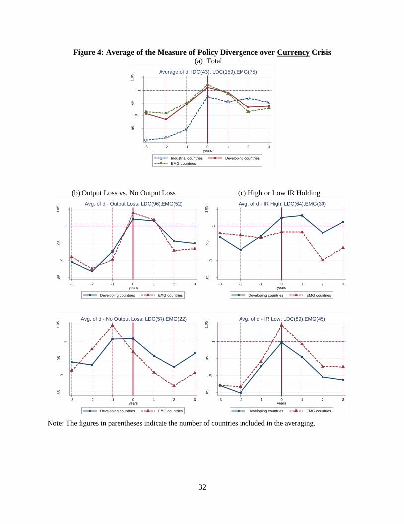
32

Figure 4: Average of the Measure of Policy Divergence over Currency Crisis (a) Total

(b) Output Loss vs. No Output Loss (c) High or Low IR Holding

Note: The figures in parentheses indicate the number of countries included in the averaging.

.85

.9.9

5

1

1.0

5

Avg

. o

f d

-3 -2 -1 0 1 2 3years

Industrial countries Developing countries

EMG countries

Average of d: IDC(43), LDC(159),EMG(75)

.85

.9.9

5

1

1.0

5

Avg

. o

f d

-3 -2 -1 0 1 2 3years

Developing countries EMG countries

Avg. of d - Output Loss: LDC(96),EMG(52).8

5.9

.95

1

1.0

5

Avg

. o

f d

-3 -2 -1 0 1 2 3years

Developing countries EMG countries

Avg. of d - IR High: LDC(64),EMG(30)

.85

.9.9

5

1

1.0

5

Avg

. o

f d

-3 -2 -1 0 1 2 3years

Developing countries EMG countries

Avg. of d - No Output Loss: LDC(57),EMG(22)

.85

.9.9

5

1

1.0

5

Avg

. o

f d

-3 -2 -1 0 1 2 3years

Developing countries EMG countries

Avg. of d - IR Low: LDC(89),EMG(45)

33

Figure 5: Average of the Measure of Policy Divergence over Banking Crisis (a) Total

(b) Output Loss vs. No Output Loss (c) High or Low IR Holding

Note: The figures in parentheses indicate the number of countries included in the averaging.

.8.9

11

.11

.2

Avg

. o

f d

-3 -2 -1 0 1 2 3years

Industrial countries Developing countries

EMG countries

Average of d: IDC(23), LDC(98),EMG(44)

.7.7

5.8

.85

.9.9

5

1

1.0

5

Avg

. o

f d

-3 -2 -1 0 1 2 3years

Developing countries EMG countries

Avg. of d - Output Loss: LDC(64),EMG(33)

.7.7

5.8

.85

.9.9

5

1

1.0

5

Avg

. o

f d

-3 -2 -1 0 1 2 3years

Developing countries EMG countries

Avg. of d - IR High: LDC(39),EMG(18)

.7.7

5.8

.85

.9.9

5

1

1.0

5

Avg

. o

f d

-3 -2 -1 0 1 2 3years

Developing countries EMG countries

Avg. of d - No Output Loss: LDC(32),EMG(10)

.7.7

5.8

.85

.9.9

5

1

1.0

5

Avg

. o

f d

-3 -2 -1 0 1 2 3years

Developing countries EMG countries

Avg. of d - IR Low: LDC(55),EMG(26)

34

Figure 6: Average of the Measure of Policy Divergence over Debt Crisis (a) Total

(b) Output Loss vs. No Output Loss (c) High or Low IR Holding

Note: The figures in parentheses indicate the number of countries included in the averaging.

.85

.9.9

5

1

1.0

5

Avg

. o

f d

-3 -2 -1 0 1 2 3years

Developing countries EMG countries

Average of d: LDC(189),EMG(48)

.85

.9.9

5

1

1.0

5

Avg

. o

f d

-3 -2 -1 0 1 2 3years

Developing countries EMG countries

Avg. of d - Output Loss: LDC(89),EMG(35).8

5.9

.95

1

1.0

5

Avg

. o

f d

-3 -2 -1 0 1 2 3years

Developing countries EMG countries

Avg. of d - IR High: LDC(70),EMG(14)

.85

.9.9

5

1

1.0

5

Avg

. o

f d

-3 -2 -1 0 1 2 3years

Developing countries EMG countries

Avg. of d - No Output Loss: LDC(89),EMG(13)

.85

.9.9

5

1

1.0

5

Avg

. o

f d

-3 -2 -1 0 1 2 3years

Developing countries EMG countries

Avg. of d - IR Low: LDC(113),EMG(34)

35

Figure 7: Average of the Measure of Policy Divergence for Latin America and Asia

Notes: “Latin America” includes: Argentina, Bolivia, Brazil, Chile, Columbia, Costa Rica,

Ecuador, El Salvador, Honduras, Mexico, Peru, Uruguay, and Venezuela. “Asia” includes:

Indonesia, Korea, Malaysia, the Philippines, and Thailand. For each of the Latin American

countries, “Year 0” indicates the year when the crisis is the most severe among the years: 1981.

1982, and 1983, i.e., it varies among the countries. For the Asian countries, “Year 0” is 1997.

.4.5

.6.7

.8.9

11

.1

Avg

. o

f d

-5 -4 -3 -2 -1 0 1 2 3 4 5years

Latin America Asia

Average of d: LAMERICA (12) and Asia (5)

36

Figure 8: Measures of Policy Divergence for Latin American and Asian Crisis Countries

(a) Latin America

(b) Asia

Notes: “Latin America” includes: Argentina, Bolivia, Brazil, Chile, Columbia, Costa Rica,

Ecuador, El Salvador, Honduras, Mexico, Peru, Uruguay, and Venezuela. “Asia” includes:

Indonesia, Korea, Malaysia, the Philippines, and Thailand. For each of the Latin American

countries, “Year 0” indicates the year when the crisis is the most severe among the years: 1981.

1982, and 1983, i.e., it varies among the countries. For the Asian countries, “Year 0” is 1997.

0.2

.4.6

.81

1.2

1.4

1.6

1.8

d=

measure

of policy d

ispers

ion

-5 -4 -3 -2 -1 0 1 2 3 4 5Year

Argentina Brazil

Mexico Columbia

Chile

0.2

.4.6

.81

1.2

1.4

1.6

1.8

d=

measure

of policy d

ispers

ion

-5 -4 -3 -2 -1 0 1 2 3 4 5Year

Thailand Korea

Malaysia Indonesia

Philippines

37

Figure 9: Average Deviations from the Means for Each Trilemma Index over a Crisis for

Latin America (a) and Asia (b)

Notes: “Latin America” includes: Argentina, Bolivia, Brazil, Chile, Columbia, Costa Rica, Ecuador,

El Salvador, Honduras, Mexico, Peru, Uruguay, and Venezuela. “Asia” includes: Indonesia, Korea,

Malaysia, the Philippines, and Thailand. For each of the Latin American countries, “Year 0” indicates

the year when the crisis is the most severe among the years: 1981. 1982, and 1983, i.e., it varies

among the countries. For the Asian countries, “Year 0” is 1997.

.2.4

.6.8

11

.21

.4

Avg

. o

f d

-5 -4 -3 -2 -1 0 1 2 3 4 5years

Monetary Indep. Exch. R. Stab.

Financial Op.

(a) Latin America

.2.4

.6.8

11

.21

.4

Avg

. o

f d

-5 -4 -3 -2 -1 0 1 2 3 4 5years

Monetary Indep. Exch. R. Stab.

Financial Op.

(b) Asia