the modulational regime of three-dimensional water waves and the davey-stewartson system

Ann. Inst. Henri Poincare’,

Vol. 14, n” 5, 1997, p. 615-667 Analyse non liniaire

The modulational regime of three-dimensional

water waves and the Davey-Stewartson system

Walter CRAIG Department of Mathematics and Lefschetz Center for Dynamical Systems,

Brown University, Providence, R.I. 02912, USA E-mail: [email protected]

Ulrich SCHANZ and Catherine SULEM Department of Mathematics, University of Toronto, Toronto, M5S 3G3 Canada.

E-mail: [email protected]; [email protected]

ABSTRACT. - Nonlinear modulation of gravity-capillary waves travelling principally in one direction at the surface of a three-dimensional fluid leads to the Davey-Stewartson system for the wave amplitude and the induced mean flow. In this paper, we present a rigorous derivation of the system and show that the resulting wavepacket satisfies the water wave equations at leading order with precise bounds for the remainder.

Key steps in the analysis are the analyticity of the Dirichlet-Neumann operator with respect to the surface elevation that defines the fluid domain, precise bounds for the Taylor remainders and the description of individual terms in the Taylor series as pseudo-differential operators and their estimates under multiple scale expansions.

Key words: Modulation, water waves

RBsuMB. - La modulation nonlineaire d’ondes se propageant principale- ment dans une direction a la surface d’un canal tridimensionnel conduit au systeme de Davey-Stewartson pour l’amplitude de l’onde et le champ

A.M.S. classification scheme numbers: 76 B 15, 35 C 10

Ann&s de I’lnsfitut Henri P&cart! - Analyse non iinCaire - 0294-1449 Vol. 14/97/05/$ 7.0010 Gauthier-Villars

616 W.CRAIG,U.SCHANZANDC.SULEM

moyen induit. Dans cet article, nous presentons une derivation rigoureuse du systeme et nous montrons que l’approximation modulationnelle satisfait les equations des ondes de surface a l’ordre dominant.

Les &apes importantes dans l’analyse sont l’analyticite de I’operateur de Dirichlet-Neumann par rapport a l’interface qui definit le domaine du fluide, des estimations du reste dans le developpement de Taylor de l’operateur, ainsi que la description des differents termes de la serie comme operateurs pseudo-differentiels et leurs developpements multi-Cchelles.

1. INTRODUCTION

This paper is a contribution to the mathematical theory of the water wave problem, and the methods of modulational analysis. Our goal is a rigorous understanding of the Davey-Stewartson system as an approximation to the three-dimensional gravity-capillary wave problem, in the modulational scaling regime. This paper extends the previous work of W. Craig, C. Sulem and P.L. Sulem [8] on the two-dimensional water wave in the modulational regime, where the asymptotic description of solutions is given by the cubic Schrodinger equation. The main mathematical contribution for the three (or higher) dimensional problem is the analysis the boundary integral operators of potential theory, which is more intricate than in two dimensions. The description of singular operators and pseudo-differential operators under multiple scale expansions is similar to the analysis of [8].

The water wave problem describes the evolution of an Euler fluid that is inviscid, incompressible and additionally irrotational, with a free surface and under the influence of the gravity and of surface tension. This is a potential flow, which is described in Eulerian coordinates by the velocity field u = Vv, where

Ap=O (1.1)

for x = (zr1,z2,zs) E {-h < 23 < q(zI,z2), (zzl,zz) = z’ E R*} the fluid domain. The bottom boundary condition is that &~(p(z’, -/l) = 0, and the c&ssicaI free surface conditions are that

atlp+;(vv)2 + 9r! - @H(v) = 0, (1.2)

a,rj+a,lcp~ a,q - az,cp = 0,

hnoles de I’lnstitut Henri PoincarP Analyst non h&k

MODULATION OF WATER WAVES 617

on the surface x3 = n(z’), where H(q) is the mean curvature of the free surface.

In the modulational regime, one derives that solutions to (l.l)-( 1.2) are described formally to lowest order in E << 1 by the expressions:

(1.3) < = 2t Re(c(Z1,Z2,7)ei(lc121--wt)) +td(z~,~,~) + O(t2).

with z1 = ~(51 - w’t), z2 = cx2, 7 = c2t, w2 = (g+,Ok$)kr tanh(hkr) and w’ = dw/dkl. The potential function Cp(x, t) is the harmonic extension of the boundary values ,$(x’, t) into the fluid domain defined by the upper boundary Fj’. The two functions (~(2, T), d(z, T)) satisfy the Davey- Stewartson system:

with constants X, p, 2, x1, ~11, y that depend upon g; k, h and /3 as specified below.

A fundamental question is in which precise sense does the solution prescribed by the modulational approximation (1.3)-( 1.4) approximate the full Euler equations (l.l)-( 1.2) which give the fluid evolution. In this paper, we give a rigorous derivation of the Davey-Stewartson system (1.4), together with an estimate of the error of the approximation (1.3), which is in the same spirit as the paper [S] on the two-dimensional water wave problem. The modulational regime is derived with the method of multiple scales (both spatial and temporal), using the basic assumption that the solutions behave independently on asymptotic separated scales. In general, the method of multiple scales involves singular pertubations, as the description of slow time and/or spatial scales ultimately results in the replacement of higher derivative operators with lower. Justifying this formal analysis gives rise to a number of basic mathematical questions, as in general the critical analytic issues involve the highest order differential operators and the behavior of solutions at high wavenumbers. A further consideration for the water wave problem is that the integral operators of potential theory for the fluid domain play a central role: under multiple scales analysis these are approximated by differential operators, and the nature of this approximation must be understood. A general theory of pseudo-differential operators and multiple scale expansions is developed for this purpose in [8], and this with several modifications will be used in this paper.

Vol. 14, no 5.1997.

618 W. CRAIG, U. SCHANZ AND C. SULEM

The original derivations of the modulation equations for three- dimensional water waves appeared in Benney and Roskes [2] and in Davey-Stewartson [IO] in the case of pure gravity waves. The effect of surface tension was analysed by Djordjevic and Redekopp [ 1 l] as well as in Ablowitz and Segur [ 11. The derivation of the nonlinear Schrodinger equation from the two-dimensional water wave problem was first obtained by Zakharov [27] in the case of infinitely deep water, and in finite depth water by Hasimoto and Ono 1151. As opposed to our analysis in [8] in which Lagrangian variables were used, we adopt in the present paper an Eulerian approach, using dependent variables defined on the free surface alone which are described in Craig and Sulem [9]. Formal aspects of the modulational analysis are thus quite similar to that of Hasimoto and Ono [ 151 for the two dimensional problem. This choice of coordinates is not necessarily optimal for the initial value problem for water waves, but they do allow a relatively clean and systematic treatment of the multiple scales analysis and an estimate of remainder terms.

Asymptotic approximations of the water wave problem have been the origin of many of the nonlinear partial differential equations of mathematical physics [22]. Because of this, there has been an effort over a number of years to understand in a rigorous way the validity of these approximations and to justify if possible the use of the asymptotic limits. Kano and Nishida [ 171 proved an existence theorem for the initial value problem for two dimensional water waves for analytic initial data and gave a rigorous analysis of the shallow water scaling limit. In subsequent papers, both Craig [6] and Kano and Nishida [ 181 addressed the dispersive long wave scaling regimes for two-dimensional water waves, giving an analysis of the Boussinesq and KdV approximations. The modulational scaling regimes are somehow harder to study, as the solution is approximated through an ansatz of a multiple scale analysis, which involves in particular the assumption of the independence of several scaling regimes, and this independence must be justified with rigorous errors estimates in the full Euler equations (I. 1) (1.2). For the two-dimensional problem, a rigorous result on the derivation of the nonlinear Schrodinger equation is given in IS]. The results in the three-dimensional modulational regime of this paper are close in spirit to [S].

There are a number of recent papers on rigorous justification of modulational analysis in several settings other than the water wave problem. The work of Collet and Eckmann [S] gives a comparison of solutions of the Swift-Hohenberg equation with a modulational approximation in the form of a Ginzburg-Landau equation. Both of these are parabolic equations. Mielke


and Schneider have also studied parabolic problems whose modulational limit gives the Ginzburg-Landau equation, and additionally to these, Kirrmann, Mielke and Schneider [ 191 have results for modulational regimes of nonlinear hyperbolic systems. More recently, Pierce and Wayne [25] studied the modulational regime for a one-dimensional wave equation which involves the interaction of left and right moving periodic wave trains. The modulational regime and the method of multiple scales are widespread in applied mathematics, and we think that a rigorous mathematical study of this approximation procedure is important to understand the nature of the asymptotic solution.

The organization of the paper is as follows. In Section 2, we describe the water wave problem in terms of the variables on the free surface (T/(X’, t), E(z’, t) = (P(x’, rj(~‘, t), t)), the Dirichlet-Neumann operator G(r/) for the fluid domain and its formal Taylor series expansion with respect to ~(2:‘). Section 3 is devoted to the formal derivation of the Davey-Stewartson system. The analysis starts in Section 4, where we give the rigorous analysis of the Dirichlet-Neumann operator and its Taylor approximation. In concise terms, we show that, for surface variations 7(:x’) in a neighborhood of zero in the C’(R2)-topology such that ]al+‘rl]~~ < cc, the operator G(n) is analytic as a mapping between the Sobolev spaces G(q) : W”+l,4(R2) -+ W”,‘1(R2) f or any 1 < q < ec. This work on the regularity of operators of potential theory under pertubation of the domain is related to early work of Garabedian and Schiffer [ 121, and to work of Coifman and Meyer [4] on Cauchy integrals. Our analysis of the analyticity of G(rj) is fundamentally based on the multiple commutator estimates that appear in the paper of Christ and JournC [3]. Section 5 gives an estimate in WR>q(R2) of a class of singular integral operators that make up the Dirichlet-Neumann operator, its Taylor approximates and its Taylor remainders. Section 6 is focussed on the mathematical justification of the formal expansion for the water wave problem given in Section 3. In part, this uses an analysis of pseudo-differential operators in a multiple scale regime, which is along the lines of [8]. As we work here in general Lq(R*)-spaces, the required additional estimates are provided.

We now conclude this introduction by discussing the form of justification of the modulational limit that we can provide. In both the two-dimensional and three-dimensional water wave problem, the modulational approximation involves solutions in the form of wavepackets of amplitude O(F), whose envelopes simply translate with the group velocity over time intervals of length O(F-I), and evolve on time intervals of length O(e-?) according to a modulational equation (nonlinear Schrodinger or Davey-Stewartson

Vol. 14. 11” s-1997

620 W.CRAIG,U.SCHANZ AND C.SULEM

equations). In order to compare a solution to the water wave problem to its modulational approximation, it is thus necessary to have an existence theorem for solutions of (1 l)-( 1.2) for initial data of amplitude 0 (F) which have time intervals of existence of 0(te2), corresponding to times O(1) in the modulated time scale. At present, there are no existence theorems for the full water wave problem, so that we are as yet unable to make the statement that true solutions (71, <) of (1. I)-( 1.2) and their modulational approximations (q, <) of (1.3)-(1.4) remain close in an appropriate norm over modulational time scales: sup o<t<q-2) II - c;rm < 4f3). In this paper, we make the alternative, and weaker statement that the approximations (6, F) constructed from the Davey-Stewartson system (1.4) result in an I error when acted upon by the nonlinear water wave operator given by the r.h.s of (1.2). If the implicit function theorem were available, these two statements would be equivalent but as it is not. the second is weaker than the first. The statement that we make is sufficient to guarantee that over time scales of interest (0 5 t < O(E-‘)), the dominant evolution of the modulational regime is described through (1.3) and the Davey-Stewartson system (1.4), and accumulated errors cannot grow to significance.

The construction of approximate solutions in the modulational regime also depends upon the well-posedness of the initial value problem for the Davey-Stewartson system (1.4). There are two choices of sign for each of the quantities a and X/p which affect this (although N < 0, X/p < 0 does not occur in the water wave problem). All of these cases have been addressed in the literature, see Ghidalia and Saut [ 131, Linares and Ponce [20], Guzman-Gomez [14] and Hayashi and Saut [16]. The nature of the solution depends importantly upon the sign of c). For a > 0, one can take co(z) E ,‘,(R’) an essentially one has solutions d (c(z,~), d(z,r)) E H”(R2) x H”+l(R2). When however cy < 0, one cannot impose zero boundary conditions for d(z, r) at spatial infinity. The solution essentially has a “wake” of infinite extent backwards along the characteristics z1 f 6~2 = Con& and d(z,r) E WTn-1.cu(R2) and not better. A local representation of the solutions of the nonlocal equations (1.2) is then problematic. Our results on the justification of the modulational approximation reflect this fact: we have results in the case (IY < 0 only for the approximate solutions of (1.3) when cutoff smoothly near (arbitrarily close to) the modulational variables x at spatial infinity. These results on the initial value problem are reviewed in Section 6, which then finishes with the proof of our main results and rigorous error estimates.


2. EQUATIONS OF MOTION

2.1. The water wave problem

We consider the movement of the free surface x = (z’, I), XI = (x1,x2) E R2, of a three-dimensional fluid with surface tension p, under the influence of gravity g. The domain is a channel which is infinite in the horizontal directions and has a fixed bottom at 2s = -1~. The fluid is taken to be incompressible, inviscid and h-rotational, so that the fluid motion is described by a velocity potential cp which satisfies:

Acp=O for - h < 23 < T/(x’, t). (2.1)

The boundary conditions are

&,(p = 0 on x3 = -h (2.2)

and on x3 = q(x’, t), which is the free surface over the fluid domain,

where

is the mean curvature of the free surface. The aim of this section is to reduce the system (2.1)-(2.3) to a system where all the functions are evaluated at the free surface only and cp and its derivatives in the interior are not used. For this purpose, we introduce the trace of the velocity potential cp at the surface

and the Dirichlet-Neumann operator acting on 1(x’), which is defined by

where d,cp is the normal derivative of ‘p on the surface. The linear operator G(v) relates (up to a normalization factor) the boundary values of cp on

Vol. 14, no 5-1997

622 W. CRAIG, U. SCHANZ AND C. SlJLEM

the surface to its normal derivative. On the free surface :x3 = q(x’. f) we additionally have that

and

&,cp =

Using expressions (2.4)-(2.6), system

&7l - G(q)< = 0

1

G(v)1 + i3,~. a,/< 1+ pzI# .

(2.6)

equations (2.1)-(2.3) are equivalent to the

(2.7)

which is an evolution equation for the elevation of the free surface 7~(:1:‘, t)

and the trace of the velocity potential on the free surface e(~:‘. t). It is this system that we will use in this paper on the rigorous modulational analysis of the three-dimensional water wave problem.

2.2. The Taylor expansion of G

We briefly outline the formal derivation of the Taylor expansion of G in powers of the surface elevation rl. Details can be found in [8] for the two-dimensional case and in [7] for the three-dimensional case. We look for an expansion of the form

G(V) = fJ Gj(V) j=O

where Gj (71) is a pseudo-differential operator homogeneous in 71 of degree j. For this, we consider the particular family of harmonic functions:

(p&d) 11:s) = eip,r’ cosh(lpl(z:~ + h)) (2.9)

where p = (pI,p2) E R2 and Ipl = dm. These are harmonic functions in {x3 > -II} which satisfy azs, ‘pr, = 0 on the bottom boundary x;:3 = -/L By definition,

G(7$pp = i&(pp - &I(P, . a,~rjls~. (2.10)

A~mdrs & l’htirrrr ffrwi Poiwo~-r; Analyse non h&ire


We substitute (2.9) into (2.10), expand the hyperbolic functions near 23 = 0, and replace the r.h.s. of (2.10) by its expansion C,“=, Gj(rl)‘pr. We obtain thus an identity, and by identifying the terms of degree j in q we get the expansion of G from a recursion formula. Using the usual notation that D4 = -i&, and IDI = (-A) I/2 the result is as follows. For j even: ,

Gj(q) = $(JlDl j+‘tanh(hlDI) - i&(#) . DIDf-‘tanh(hlDI))

- c (<J i r”e*l - c (<J ( “‘id For j odd:

WV) =

-

-

(2.11)

@D[j+’ - i&&f). DIDI+)

! eYen

c i<j &Wii)vi’lDl’-‘. (2.13)

1 odd

In the analysis of this paper, we need the explicit form of the first three terms of the expansion, namely

Go = IDI tanh(hlDI) (2.14)

G,(rj) = D T/D - GoqGo (2.15)

%(7/l) = -f (Goq2/D12 + ID12r12G~ - 2Gorr%rlGo). (2.16)

This form of analysis of the Dirichlet-Neumann operator is useful in a variety of settings. For example, we have used it in a method for numerical computations of time dependent free surface flows [9], and de la Llave and Panayotaros [21] in a similar context have derived the Taylor expansion of the Dirichlet-Neumann operator in the context of water waves on the surface of a fluid layer surrounding a gravitating sphere.

Vol. 14, no 5-1997.


3. FORMAL DERIVATION OF MODULATED SOLUTIONS

This section is devoted to the formal modulation expansion, leading to the Davey-Stewartson system. This derivation starts with the form (2.7)-(2.8) of the water wave problem, but in other respects follows the general method of multiple scales. The modulational regime considers small amplitude solutions of (2.7)-(2.8); the linearized system around water at rest is

L; =o 0

(3.1)

with

The system (3.1) admits solutions of the form:

c eiv + cc, < = c e+ + c.c + d (3.3)

where cp = k . Z’ - wt. We use c.c to denote the complex conjugate of the preceding terms. The constants c and d are arbitrary, while the wave vector k = (ICI, 52) is related to w by the dispersion relation;

w2(k) = (g + ~lk12)11cI tanh(hjkl). (3.4)

We study a scaling regime suitable to observe a packet of nearly one- dimensional waves ( Ik2 1 < llcr I) t ravelling in the zr-direction. We suppose that the waves have small amplitudes and that the effect of the nonlinearity will be to modulate the amplitude c which becomes a slowly varying function of space and time. To this end, we introduce a multiple scale expansion, with a large scale spatial variable X’ = (X,, X2) = TV’ = e(zr,za) and two slow times T = Et and r = c2t, and we expand the solution in the form

7 I.= q(l) + ,242) + . . .

(3.5) ( = ,p + ,2p + . . .

and G = G(O) + &J(l) + . . .

Annoles de I’lnsfitut Hrnri Poincard Analyse non Ii&ire


At leading order, we have

,,(l) = iw O-Pkf

c(X, T, T)e+ + c.c

t(l) = c(X, T, 7-)e+ + c.c + d(X, T, T). (3.6)

From the preceding paragraph,

p = klxl - wt and w2 = (g + ,f?kf) ICI tanh(hkl).

For concise notation we will use the notations in the following calculations: x = hkl, g = tanhx. Furthermore, Dj = Dy) + ED:‘) where derivatives me D!‘) = &a,. and Dj’) = iady, (j = of ]D[ and t”,ni(hjDl)

1,2). We first write the expression using results of [8] on pseudo-differential operators

in a multiple scale regime, obtaining

IDI = 10$O)f + E~~)I~~“)l-lD$l) + $D$O)I-~D!~)~ + o(2), (3.7)

tanh(hlDI) = tanh(hlDp)I)

+ thD~)ID$“)l-l(l - tanh2(D$“)))D$‘)

+ E2 (

$D$“)lp’(l - tanh2(hDp)))DL’)’

- h2(1 - tanh2(hDy))) tanh(hlDp)I) Di’)” >

+ O(E3) . (3.8)

To obtain the coefficients G(“), we first write the expansion of G in terms of powers of v (see section 2.2) and then use the expansion of v in t together with (3.7)-(3.8). At leading order, we recover

G(O) = Dp) tanh(hDy)). (3.9)

The terms of order E and t2 are respectively

G(l) = D~“)71(1)Djo) - G(‘)v(l)G(‘) + tanh(hDp))Dil)

+ hD$‘) (1 - tanh2( hDy))) D{l) (3.10)

Vol. 14, Ilo 5-1997.

626 W. CRAIG, U. SCHANZ AND C. SIJLEM

and

(3.11)

+ @4rl(2)@“) - @),rl(*)G(0) + Df$,(l)~i~) + @q!‘)@“’

- G(“)v(l) ( titnh(hDiO))Dil) + hDp) (1 - tal~h2(hD10)))D~‘))

- ( tanh(h,D~))D{l) + hII{‘) (1 - tanh2(hD10)))Dr’))~(1)G((1)

G(o)7/(1)“Df’)2 + D, (“)2,1(1)2G(0) - 2G(0)7/(1)G(“)11(1)G(“)),

We now expand equations (2.7)-(2.8) in powers of t, which at order n for 11, > 1 gives the inhomogeneous linear system;

(3.12)

The solvability condition requires that the r.h.s. of (3.12) is orthogonal to the kernel of the adjoint operator

The kernel of L* is spanned by

(3.13)

(3.14)

thus the solvability conditions are equivalent to the following two conditions: (Sl) A, does not contain terms independent of p (S2) The coefficients I’, and Q,, of e ‘9 in A, and B,, respectively satisfy

At order 2, we have

A2 = -,$’ + @E(l) (3.16)


Using the expressions of 17 (l) E(l) and G(l) given in (3.6) and (3.10) we get: ,

AZ =i - (cr + X(1 - CJ2))C~& eiP

(1 - (T tanh(2X)) eziP + CC

+ ~kfc’(l + cr2)e2i9 + c.c

At this order, the solvability condition is that

a+X(l-a’)+- 0 (3.17)

or equivalently,

CT + ‘d’c<& = 0 (3.18)

where w’ = &,w(/~r,O). Thus c = c(zl, ~2, Q-) with zr = X1 - w’T, and z2 = X2. This expresses that the wave packet travels with its linear group velocity w’. The system (3.12) at order 2 is solved in the form

rjc2) = pleip + y2e2+ + c.c + p3

tc2) = qle@ + q2e2ip + c.c + q3 (3.19)

with

1 1 Pl = -CT + -(a + X(1 - (T2))Q,

g+m: (CT” - 3):;

pz = a(pkf(a2 - 3) + a2g) c 2

41 = 0

q2 = iwkl(z*(l - CT”) + 3(1+ ,z,,) 2

4a(/%~(c72 - 3) + Sg) c

py = i(k:(c’ - l)lc12 -d*).

The dependent variable q3 can be chosen equal to 0, and c and d, are slowly varying functions which are not determined at this stage of

Vol. 14, n” 5.1997

62% W. CRAIG, U. SCHANZ AND C. SULEM

the expansion. Note that the denominator of p2 and q2 vanishes when /3rq(ff2 - 3) + n2g) = 0. This is known as the second harmonic resonance [Ill. At wavenumbers satisfying this condition, the analysis breaks down and a new scaling is required. A formal analysis of this regime can be found in the article of McGoldrick [23] and we do not discuss it in the present paper.

For wavenumbers such that Plct( a2 - 3) + m2g) # 0, we have at order 6:‘:

The elimination of the p-independent term in A3 leads to:

--PST - hdx,s, - hdxs, 2Wki

- -Iclf, = 0 9 + PG

or equivalently

(3.20)

(3.21)

(3.22)

with 2wglq

01 = g+Pk-T

+ w’(1 - g2)kf.

Using (3.18), we see that U = dT + w’dX, satisfies the homogeneous wave equation

In the limit T large, or equivalently 7- = O(1) (which is the regime that interests us), U = 0, therefore we might as well assume that d, similarly to c, is a function of zl: z2 and r only. Equation (3.22) thus reduces to

(gh - J2)dzm + ghd,,., + NIIcI:~ = 0 (3.23)

For wave numbers such that w’~ = gh, (3.23) is singular and a different scaling has to be used [ 111. In the following, we assume that this coefficient does not vanish.


To express the solvability condition (S2) we write P3 and Q3 in the form

p3 = -PIT -

- h(l - a2)(1 - XCT)C,,,~ + k:(l - a2)p3 c

- f$$ (1 - f7 tanh(2x))c*q2 - k::(l+ a2)c*p2

+ wkl -cd,, + k’aw2 9 + Pk: (9 + /Jkf)2 (-1 + 2g tanh(2x)(c(2c)

Q3 = - c, - iklcd,, - 2kF (1 - g tanh(2x))c*q2

-t- %(I - 2atanh(2x))/c12c

Solvability conditions (SI)(S2) read

2ic, + xc,,,I + 1uczzz2 = xlc12c + x14, ch,z, + A,,, = -rlcl:, (3.24)

where, using notation similar to Ablowitz and Segur [I], the constants are given in the following list:

X = d;lw(kl,O) z w”

11, = w//k1

k; x=z

(

(1 - (r2)(9 - a2) + /5(3 - a2)(7 - 0”)

CT2 - &3 - CT”)

+ 8~~ - 2(1 - a2)2(1 + 3) - % 1+P >

x1 = -kl 2 + (

%(l - a2)(1 + li,)

Q = gh - w12

gh kl

‘-Y = gh (

2w9

g+/?kt + ~‘(1 - g2)k1

> /y - k’:fi

9

Vol. 14, no 5.1997.

630 W. CRAIG. U. SCHANZ AND C. SULEM

Equation (3.24) is the Davey-Stewartson system for the modulation of a solution to the water wave problem, with underlying spatial wavenumber h:. Finally, the system (3.12) at order 3 can be solved in the form

with coefficients Sj, 6:. j = 1 . . .7 depending on w, k, h and y. This establishes on a formal level that at leading order the interface

deformation and the potential velocity on the surface have the form

with cp = krrcl - wt and w* = (9 + pI$)k, tanh(hkr). The amplitude c of the wave packet and the potential d satisfy the Davey-Stewartson equations (3.24) in the slow variables r = r2t, z1 = e(zr - w’t) and z2 = ~2~. The coefficients X, p, x1, x, 0 and y depend on the gravity y, the depth h, the surface tension /3 and the wave number ICI r, as described in the above list.

4. ANALYSIS OF THE DIRICHLET-NEUMANN OPERATOR IN THREE DIMENSIONS

The purpose of this paper is to supply a rigorous basis for understanding the above formal procedure, which consists of several modulational scalings and the formal derivation of the Davey-Stewartson system (3.24). As posed in equations (2.7)(2.8), the water wave equations form a nonlinear system of integro-differential equations in the free-surface variables (x:‘, t). In contrast, the Davey-Stewartson system is a nonlinear system of partial differential equations, and it is evident that the modulational approximations consist in part in approximating integral operators by partial differential operators. The central integral operator for the water wave problem is the Dirichlet- Neumann operator G(*q). The analysis of this section is focused on the description of G(q) and its dependence upon the fluid domain, through the function n(z’). The three basic facets of the analysis are (i) the analyticity of G(q) in I, and approximation of it by its Taylor series, (ii) the


description of the Taylor remainder terms and their estimates, and (iii) the description of the individual terms in the Taylor series for G(q) as pseudo- differential expressions, and estimates of their behavior under multiple scale expansions. The latter topic was addressed in a general setting in a previous paper [8]. We set about now to describe the former two.

4.1. An exact implicit formula for G

The fundamental solution of the Laplace equation in the domain {x E R3 : z3 > -/l} which satisfies Neumann boundary condition at z3 = -h is given by the method of images;

T(x:y)=-1 ~ ~ 4T ,xly, + ,x’y*, ’ xJER3 ( >

(4.1)

where y* = (Y’; -(2h + ~3)) is the reflection of y with respect to the bottom plane 23 = -h. For x = (z’, r/(x’)) at the surface (with X’ E R2) we denote the unit normal by

N(z’) Ix (1 + (az,g)-1’2 -7’” . ( >

Write the boundary values of a harmonic function p(x) as ((2’) = (p(z’, r~(z’)), and use Green’s identity for a point (x’, rl(z’)) at the surface, to find

- s (W/K) (Y’)~(x, Y) dy’, (4.2) R”

where we are using the notation that x = (z’, 7(x’)), Y = (y’, v(Y’)). At the surface, we rewrite the Green’s functions

1

+ (Id - y’12 + (2h + q(d) + ~,(y’))~)‘i~ > (4.3)

Vol. 14, no 5.1997.

632 W.CRAIC,U.SCHANZ AND C.SULEM

and the double layer potential

which can be written as

-r(z,Y) = & ( lx/ T y/~ + (lx;/ _ yt[21+ 4h,2)1/2

> + ;p. y’) (4.5)

and

We denote the quotients in the above two expressions by

Q(v) = VW) - ‘l(Y’) lx’ - Y'I

rl(x') + rl(Y') Ql(V) = (Ix:’ -ytl2 + 4fL2)1/2:

(4.7a)

(4.76)

obtaining the following expressions:

e(x’, y’) 1 1 =G p _ yIJ

( 1 (1 + Q2) l/2

-1

>

+kT 1

(lx’ - y’)2 -+- 4h2) 1’2

x ( (1 + &l ,,;.,.,::,,.)l,2 + Qfy2 - l . > (4.8) Using the fact that

(x, _ y,) . a,,62 = v(x’) - 77CY’) - (2;’ - Y’> . %4y’)

Ix' - Y'I (4.9)


and

(x’ - y’) . b)y,Q1 + 4h2Q1

Id - y’/2 + 4/L* = 7(d) + q(y’) + (d - y’) &~7j(‘y’)

(Id - y’12 + 4h2)‘i2 (4.10)

the term m(z’, y’) can be written in the following form.

+., y,) = _ _f_ (x’ - Y’) .a,, Q ' ', 27r 15’ - y’l2 (1 + &2

4h2Q1 (Id - y’12 + 4h2)2

’ (1 + &I ,;;,;:;:,,;, + Q;))"'") 1 2h

+ %(I z’ - y’l* + 4h2)3/2 (4.11)

’ (1 + &I I.;,;:;4h>,:1 + &?I):"* - 1 >

This will be used in the analysis of Section 4.2. We substitute these expressions in (4.2), obtaining

1 2h cb’) =G (142 + 4h2)3/2 * E

+ ii m + (/x/l2 + 4h2)lj2 (

1 1

> *G(v)<

+ M(v)< + L(v)G(rlK. (4.12)

with the two operators given by the above kernels,

W71)/44 = J DEW, YMY%Yl,

I/(7/)&‘) = 1 qd, y’)p(y’)dy’.

Denoting by 3 the Fourier transform operator, the convolution operators in the above expression are given explicitly by

F ( > & = 27w’ (4.14)

Vol. 14. no s-1997


and

3 211,

(142 + &2)3/2 >

= 2Te-2’L’p’ (4.16)

(For completeness, we give a thesaurus in Appendix A.) Equation (4.12) takes the form.

(1 - e-2h’D’)t-M(rl)l = lDl-l(l + t~-2”‘D’)G(~$oL(~)G(~)~ (4.17)

or equivalently:

(4.18)

and

B(Q)< = -(l + e -2h’D’)-‘pp(T/)C (4.19u)

A(q)< = -(I + e -“h’D’)-lplM(,f-l)< . (4.190)

Identity (4.18) is the implicit form of the operator G(r)) that we will use. Since both M(r/) and L(q) start at least linearly in q, (4.18) gives directly that GO = IDI tanh(hlDI).

4.2. Error terms in the Taylor expansion of G

Starting from the implicit formulation of G obtained in the previous section, we rederive the first three terms in the expansion of G together with the explicit form of the error. Although this derivation is more complicated that the one presented in Section 2.2, it allows us to write precise estimates on the error terms.

The Taylor expansion of the kernel lj(:z’; T/‘) defined in (4.8) is given by:

1 Py+‘,,K?) + L &+dQl, (,,hy’,LL)‘iL 1. +- 27r 12 - y’l 27r (Ix’ - T/l2 + 4h2)1/2

(4,20)


Using the relations (4.9)-(4.10), the Taylor expansion of the kernel m takes the form ‘m(3:‘: y’) =& c

_ (

(x’ - y’) . +mj(Q)

lCj<J Ix’ - y’l2

+ (x1-y’)+Q1 +

(

4h,2Q1

lx’ - y/y + 4h2 (Ix’ - y’l2 + 4h2)2 >

’ ‘+l (

4h Q13 (lx/ _ y/~2 + &2)1/2

>

1 2h

+ %(I x’ - y’12 + 4h2)3/2 nj Q1, (lx/ _ ,,I:“+ &2)1,2 ( >>

+ L (x’ - Y’) . %,4+,(Q) 27r Ix’ - y’l2

+2- ( (

x’ - y’) . i&Q1 + 4h2Q1 27r Ix’ - y’12 + 4hz2 (Ix’ - y/l2 + 4h2)2 1

’ $--1 ( Ql, (lx/ _ ,!I:“+ &2)1,2

1 (4.21)

1 2h

+ !G(I x’ - ?/‘I2 + 4h2)3/2 ny ( ‘I’ (lx1 _ ,!,i”, &2)1,2 ’ > The functions pj, qj, mj and nj are homogeneous polynomials of degree

j in v(x’) and q(y’). The expressions py, q:, m:, ny are Taylor remainders that come from Taylor expansions of (1 + n)-l12 and similar expressions, so that p:(g) N 0(&) f or small cr, and analogous estimates hold for the other quantities in their arguments.

Using (4.20) and (4.21), we write

-4~) = A,(v) + . . . + -41(v) + A: B(77) = h(v) + ‘. + BJ(rl) + @,

(4.22)

with

4(v)< = - MC1 + e -29-i; (I( W -l~~~%~~Q))Codyr

+kJ( (5’ - Y’) . QQ1 2

Ix’ - y’12 + 4h2 + (lx’ -;t,2Q; 4h2)* >

x nj-l(Ql, (lx, _ ,,,r’: &2)1/2 )<(?l’)‘Y

+ 217i. /’ 2h

(Ix’ - y/p + 4h2)3/2

’ ?Lj(Ql, (lx1 _ ,,I?+ 4h,2)l12)E(Y')dd > (4.23)

Vol. 14, no 5.1997.

636 W.CRAIG, U. SCHANZ AND C. SULEM

and

Bj(rg = - p/(1 + p-2fllyl (4.24)

P.7 (Q) 4.,(621> ih

(~&y’l’f4~‘)‘i’ 1

IX’ - ?J’I + (ICC’ - y/12 + qh,2)1/2 ~(Y’)‘Y’.

We denote by A: and BT the terms which describe the Taylor remainder. For our purposes, we need to study the third order expansion. From (4.18), we get

G(v)E = GE + (BIGI + A,)<

+ (&Go + &Al + A2 + B;Go)< + R,(q)<. (4.25)

where the remainder R3(7~) has the form

fi3(71) = (B;‘+ BlB2 + BzBl + BlB,X + B:B1 + BzB;’

+ @B2 + (Bf)2 + B;)Gcl + (By + B;)A,

+ (1 - B)-l(Af + BA2 + B2Al + B3Go). (4.26)

THEOREM 4.1. - The Dirichlet-Neumann operator can be nv-itten in the form:

with

G(r)) = G,-j + Gl(rj) + Gz(r/) + R,(q) (4.27)

G,, = IDI tanh(hlDI)

G1 = D .7jD - Gor/Go

G2 = -;lD12q2G,, + GovG,rlGo - +,i?lD12 (4.28)

with the remainder R,(r)) dejned in (4.26).

Proof of Theorem 4.1. - We will derive the explicit form of the operators AI, A2, BI, B2, in order to express G1, G2

A,(r))< = - ID/(1 + c:-- ‘h/D -1 )

1 x%r,

(X - y’) . 3,f7/(y’) - (7jf:x’) - 7/(y’))

IT;’ - yJ’13

+ (cc’ - y’) . i)yq(y’) + 7/(d) + rj(y’)

((21’ - y’/2 + 4/x2)3/2

12h’ f& (1%’ - y’l2 + 4h2)2 1 dy’

(4.29)


We can write these expressions in terms of Fourier multipliers (see Appendix A)

A,(Q)< = D. rlD[ - lDl(l + e-2h’D’)-1qlDI(1 - e~‘~‘~‘)<

= D . ,rlDE - lDl(l + e-2hlDI)-1q(1 + e-2hioi)G0<. (4.30)

Similarly, &(q)( = -lDl(l + e-2h’DI)-1

1 ( >/

2h X --

2r ’ (Id - y’12 + 4h2) 3,2 (M) + dY’))<(Y’WY

= ID/(1 + e -2w-1 (Ile-2wlJ + e-2hlDlrl[). (4.31)

Thus, combining (4.30) and (4.31), we get

G(rl)t = (&Go + A,)I = (D . rlD - Go~Go)<.

For G2, we have

(4.32)

with G2(rl)E = (&Go + &AI + A2 + @o)E (4.33)

Am< = -jDj(l + e-2hlDI)-1 1

X- 2n

(-6h,) (z’ - Y’) . +rl(Y’) + VW) + rl(Y’) & (Ix’ - y/p + 4h2)2 1

3hQf 2

- ( 12’ - y’l2 + 4h2)3/2 1 - 12’ - ;I! + 4h2 >>

E(Y%Y

= -ID/(1 + e-2hlDI -’ qiD. e-2hlDi((dy,q)[) ) (

+ iD. ~~~~~‘((d,~rl)rp$) - &(q”(l + 2hjD))e-2hlDI

+ 2q(l+ 2hlDl)e-2hiDiq + (1 + 2hlDl)e-2hlo1q2)<

+g v2 (( -$(l + 2hlDI) + ~h2/D12)e-2hiD~<

+ 211 (

$(l+ 2hlDI) + &h21D12)rjep2”i~~[

+ ;(l + 2hlDI) + $h2jDj2

= -/D/(1 + e -2h,D,)--1 (,D e-2h1D177D

+ .!D . e-2hlDIr12D + ~~21D12e~2h~n~ 2 (4.34)

Vol. 14, Ilo 5.1997


1 + 2(1 d - 11’12 + My2 (71(x’) + ,7(1/l))’

G/i2 (Ix’ - :(/‘I2 + 4h,2)5/2 (7/(x’) + r,(yl;)z [dy’

>

= +)I(1 + e--2hIUI)l;(T,2,~,(~ + f~-‘w)

+ ‘&]lDI(-1 + CahlDl )7] + p/(1 + “-2’+-yT,2)E (4.35)

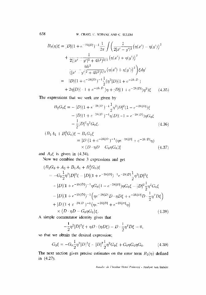
The expressions that we seek are given by

= lDl(l + e-2’“10i)-l(7,e-2h1L)1 + e-2/41,Il)

x (D . r/D - Gor/Go)[ (4.37) and A,( is given in (4.34).

Now we combine these 3 expressions and get

(B2Go + A2 + &Al + @GO)<

= -Go;rlalDI’< - lDl(l + ~-2ii1~1)1C-2irD1~02,nl’~

+ pq(1+ e- 2hiDi)-17,Go(l + e- 2hlDl)~GO~ - lD12;r/2Gil<

- pIq1+ c- WDI)--1 (T,e- 2hlDID. +$ + c- 2’b1D1D. A7”D< 2’ >

+ lDl(l + e --2hlDI)-l(~,e-2hlDI + e-w4

x (D 7/D - G07/G0)(. (4.38) A simple commutator identity gives that

-;7j21D12< + 7/D. (7/D<) - D. ;r;lD< = 0;

so that we obtain the desired expression;

G& = -G&Dj2[ - ID12;q2G,,< + GorjGor/Go. (4.39)

The next section gives precise estimates on the error term &(7/) defined in (4.27).


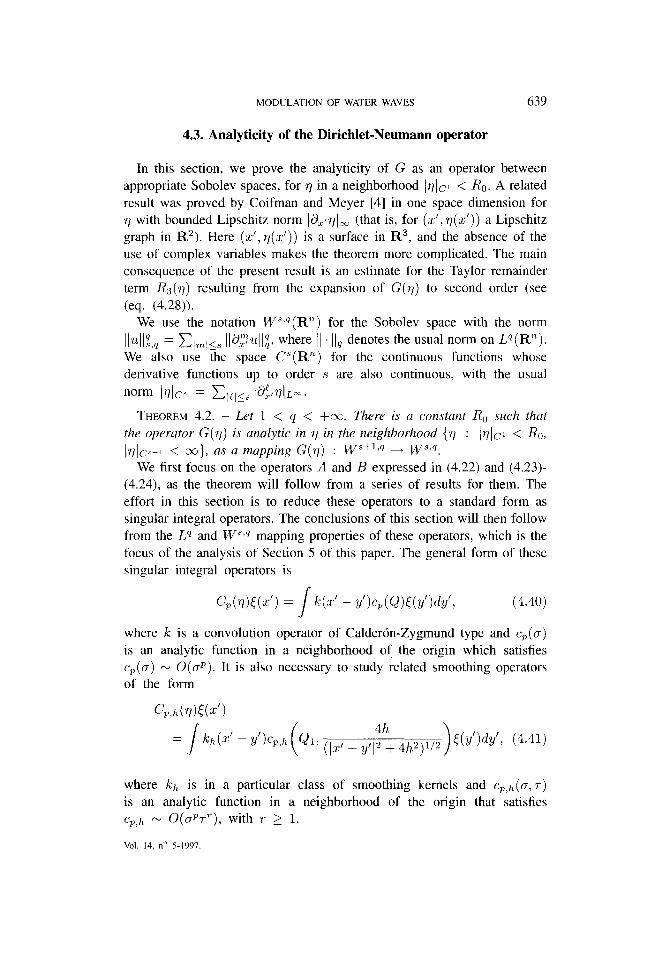
4.3. Analyticity of the Dirichlet-Neumann operator

In this section, we prove the analyticity of G as an operator between appropriate Sobolev spaces, for v in a neighborhood ]r/lcl < Ro. A related result was proved by Coifman and Meyer [4] in one space dimension for q with bounded Lipschitz norm j~Y,tql, (that is, for (x’, Q(x’)) a Lipschitz graph in R2). Here (x’,Q(x’)) is a surface in R3, and the absence of the use of complex variables makes the theorem more complicated. The main consequence of the present result is an estimate for the Taylor remainder term R3(q) resulting from the expansion of G(q) to second order (see (eq. (4.28)).

We use the notation Ws,q(R1’) for the Sobolev space with the norm ll43,, = c,n,,<s Ilmll:~ where 11 . /I4 denotes the usual norm on Lq(R”). We also use the space CS(Rn) for the continuous functions whose derivative functions up to order s are also continuous, with the usual norm MC- = Clplss IGrlb.

THEOREM 4.2. - Let 1 < q < foe. There is a constant Ro such that the operator G(q) is analytic in v in the neighborhood {rl : Jrl(cl < R,, I’I~IC:~+I < CQ}, as a mapping G(q) : Wsfl,q + W’,q.

We first focus on the operators A and B expressed in (4.22) and (4.23)- (4.24), as the theorem will follow from a series of results for them. The effort in this section is to reduce these operators to a standard form as singular integral operators. The conclusions of this section will then follow from the LY and Ws’q mapping properties of these operators, which is the focus of the analysis of Section 5 of this paper. The general form of these singular integral operators is

Cp(q)((d) = I’k(d - y’)c,(Q)<(y’)dy’. (4.40)

where k is a convolution operator of Calderon-Zygmund type and cP (a) is an analytic function in a neighborhood of the origin which satisfies CP (0) - O(#). It is also necessary to study related smoothing operators of the form

ZZ .I

. k&x’ - Y’)Cp,h 01, CIx, _ y,lf’: 4h2)1,2 t(Y’)dY’: (4.41) ( >

where k.h is in a particular class of smoothing kernels and ~~,!~(g, 7) is an analytic function in a neighborhood of the origin that satisfies Cp,h N O(CT%‘), with T > 1.

Vol. 14, Ilo 5.1997.

640 W.CRAIG. U. SCHANZ AND C. SULEM

THEOREM 4.3. - Let 1 < y < +oo, and 0 2 s E Z. The operators B,J and BT dejined in (4.22)-(4.24) satisfy the estimate:

(i> llB~(~)~ll~,~ I: I4$‘(C(~)ldc~+~ lllllq + l40 IIdls,q) (3.42) (ii> IlfT(~Mls,, L I7&‘(~(~)l7~l0+~ 11111, + Mc~ Illlls,s) (4.43)

COROLLARY 4.4 (i) The powers of B satisfy

IIBj(q)tlls,, I Iv&? (hb Il~lls,p+C(~)(l+co)j~~l~lc~+l ll~lh) (4.44)

(ii) For 17/lc1 small enough, the operator (1 -B) is invertible and satisfies

IIP - W’EIL 5 1 + (CC5I7b+l IIEII, + lrllcl ll~lls,q) (4.45)

Proof of Theorem 4.3. - First of all, we notice that the operator (1 + ~‘~loI)-~ is bounded in W”‘Q for all 1 < q < +CX and all s > 0, and furthermore

IDI = - 2 iD,jlDI-1 . iDj = -2 Rj(D)iJ,,I (4.46) j=l j=l

where Rj(D) are the standard Riesz potentials which are also Lq-bounded. Thus, to find a bound for Bj defined in (4.24), we are led to consider two types of integral operators Pj and Qj,h defined by

P,(rlK = &: , I' Iz, 1 y,l~~(Q(dKt~'~dyl (4.47)

where pj(Q) = UjQ’

(4.48)

x qj Ql(v)> o2, _ y,lf: 4h2J1,2 ( 1

~(Y%Y

We rewrite Pj in the form:

+ QI(~‘) J

,z, J y,12 Q”-1 IVY’ >

(4.49)


which is a sum of operators Cj(q) defined in (4.40) with kernel

and az:V(x')cj-l(V)

which involves the kernel k(z’ - y’) = (l/lx’ - y/I”). Similarly, and less delicately, we may write

- (4h)yz: - y:> Qjth)l= c by’ / (Ix/ _ y,12 + 4h2J71 Q:(v) E(Y’)~Y’

+ c b$?‘&: 7/(d) .I

(4h)-

(Ix’ - y’12 + 4h2)r?

x Q;-‘(v) E(Y’)~Y’ (4.50)

with coefficients derived from the binomial expansion. These are clearly in the form of operators of type C,,, (77) with smoothing kernels Ich (x’ - y’) = (l/(/z - y/j2 + 4h2)“f’) or kh(l~ - y) = ((x: - yg)/(lz’ - y’12 + 4h2)r”).

We have achieved the form for which the L’J and IV’,4 transformation properties of singular integral operators may be used. Applying Theorem 5.7 to the operators I’3 (v) and Theorem 5.8 to Qj,fL (17) of Bj (7)) we see that the estimates (4.42) hold. The operators B:(n) do not have kernel which are homogeneous polynomials in Q, Q1, but rather analytic functions of Q and Q1, and the corresponding result (4.43) follows from Theorems 5.1 and 5.2 respectively.

Pvoc?fof Corollary 4.4. - Noting that B = Bf, we have the estimate that

IIw7Klls,rl I ~m/lc~+~ 11111, + IVlCl IllllS,~I (4.51)

To prove estimate (4.44), we will proceed by induction. Suppose that

Ii@(d<lls,q I: k&l ~~<~\s,q + C(s)(l + ~o)j-lk~&l lvlc~+~~~lllq (4.52)

and let us prove that the same estimate holds for EP+l (7). Applying (4.5 1) to B(q)<, we have:

lI~j+1(77m,q I Irll~~1(1171c~ IIwIKllb.q + cl+ ~~~~-‘~~~~l77lc~+~II~~17>111~~

5 l77ljc;‘~l~lc~~l~/lc~IIIIIY,~ + ~~~~~lrllC”+‘l77lC~ll1lln~ + (1 + ~“~~-l~~~~~lrllc~+~~~l~l~~ Kllg)

5 l&1 (Ivlc ll5lls,q + C(s)(l + G)%Ilcs+~ 11111,) and estimate (4.44) on Bj is complete.


Within the region of convergence of the geometric series Cj 1,q/$, and C,(l+ CO)J-llql$l, that is for /~]cI < l/(1 +CO), we have convergence of the Neumann series for (1 - II-l. This is our first condition on I?/Ic.l, that R0 < l/(1 + CO). We now turn to the family of operators A,(Y]). To obtain the correct dependence on the smoothness of r](x), we will use the following general lemma.

LEMMA 4.5. - For :I: E R”, X(Q) un odd continuous function qf Q and r/ E Cl(R”), we huve

Proof of Lemma 4.5. - Denote B,(z) a ball in R’” of radius t and center :I; and S,(x) its boundary. Then, for any ri.< E Cl(R”),

The second term of the r.h.s of (4.54) vanishes, as the vector held is divergence free in R’” - I?,. Consider now the third term in (4.54). For < continuous the difference between this term and

I 1

, ,$, (x) I:I. - :!pl Rods,

is of order O(t), hence it suffices to consider the latter. By the mean value theorem,

~SY (4.55)

for some z = TX + (1 - ~)y , 0 < 7 < 1. Assuming that 8,~ is continuous, it suffices to consider the following integral


as the difference between (4.55) and (4.56) is again O(E). However the integral in (4.56) vanishes, as R(.) is odd, as is its argument.

Remark. - This argument uses the fact that q E Cl(R) is an essential way, and will not extend directly to q E Lip(R). However by an approximation argument it is easy to see that we may take [ E VVSJ(R”).

THEOREM 4.6. - The operators A.1 and AT dejined in (4.23) and (4.25) sati$y the estimates:

(9 llA~(~)~lls,, I C(~)lvl$~( lvb+~ Il~~~Elln + l7b ll&~~EII.s.n) (4.57)

(ii) llA~(rl)lll.s,q 5 C(s~)lvl$l ( lrjlCs+l Il&~ElL, + I7h~ Il~J~~Ells,p) (4.58) Proof of Theorem 4.6. - Using Lemma 4.5, the problem is transformed

to a situation very similar to that of Theorem 4.3. We have

A,j(q)<(z’) = - &(I + c~“‘~‘)-~ CL!,(D) 1

a x d,!r ( .!

2;’ - y’ Id - y’l2 . f%!?i(Q)E(Y’)dY’

+ &I, .i(

(x' - Y') . q/d21 + 4h2Q1

Ix' - y'l2 + 4h>2 (Ix’ - y/j* + 4h*)*

’ nj-l(Ql; (lx, _ yf/:t 4h,2)1/2 )I(Y’)dY’

+ 3,rz J’ (lx’ - ,qf h, 4h2)3/2

’ nj(Q1, (I,y _ ,,I?+ qh,2)1/2 )‘t(Y’)dY’ >

(4.59)

We use Lemma 4.5 to rewrite the relevant part as a sum of operators of the two forms. The most sensitive terms are the singular integrals

=- 7nj(Q)dy:I(Y')dY'

+

J

(xi - y;)(d - y') ICE' - y'l4 . (2mj(Q) + m$(&)&)~y~E(~‘)d~’

- iJz; v(2) .I’

z’ - y’ Ix’ - y’l”

.7n;(Q) i3,r((y’)dy’, (4.ciO)

which are of the form of the operators Cj(7l)8~~( defined in (4.40). The second and third terms of (4.59) consist of smoothing operators. The issue

Vol. 14, no 5.1997


Terms which do not involve derivatives of Ql(rj) are safe already. The terms which involve derivatives of QI(q) give rise to the following four possible integrands;

where

aJd)l = q/~V(Y’)

(Ix’ - y’,2 + 4P)W + (7/(X) + q(y’)) (d - y’)

(,:I:’ - y’,2 + 4P)“P ’ &.; r)(d)

‘3X:” = ( l2/ - ?/‘I2 + 4/$)1/z - (7)(:L-) + q(y’)) (xi - y;)

( [:I;’ - f,” + 4h,2)“/2 ’ dyr](y’)(:I:: - yg

3y’3r:Q1 = - ( IJI;/ __ !,‘I2 + &2)“/2

_ 3 (7/(x’) + ‘II(y’))(:d - y’)(x( - y;)

( ,:I? - ?/‘I2 + 4h2)5/2 + 8,1;7)(.d)(d - y’) + (q(d) + T)(tJ’))e;

(,:r’ - yq2 + 4@)3/2 j

where et is the %I” unit vector. These smoothing operators are of the form CP,fL(n)< studied in Section 5, that have already appeared in the analysis of Bj.


The operators A: resulting from the Taylor series remainders of the expansion of A behave similarly. These kernels contain functions of Q and Q1 which are analytic in their arguments and the results of Section 5 are designed for this situation.

We conclude this section by stating the result that gives an estimate of the remainders RI, Rz and 123(q), which are defined in (4.26) and (4.27). from the Taylor expansion of G(q) to the first several orders.

THEOREM 4.7. - Consider 1 < q < +oo and 0 2 s E N. Let jrll~~ < R, and I&+I < +cc The Taylor remainders R3(71) from the expansion of G(r/) .j = 1,2,3 satisfy

llWMs,s 5 Wl&;1 (lrllcl Illlls+~p + lrllc~+~ lItIll>,) (4.62)

5. ESTIMATES OF SINGULAR INTEGRALS

This section is focused on the analysis of the singular integral operators that are described in Section 4, and which make up the components of the Dirichlet-Neumann operator. Although the majority of this paper concerns two-dimensional surfaces of fluid regions in three dimensions, here we will give general results for n-dimensional singular integrals. The two basic operators are

WrlN4 = .I’ k(x - Y)c,(Q(~/))~(Y)~Y> (5.1) R”

where k(z) is a convolution kernel of Calderon-Zygmund class satisfying the so-called standard estimates for 6 > 0:

(5.2)(i)

(ii) ‘dx,y E R”, with IX - yI 5 $rl.

The expression Q(q) = (q(z) - v(y))/lz - yl is the ubiquitous difference quotient. The kernel is specified by the function cP(z), which is assumed to be analytic in the ball Iz I < RO and to satisfy cp(z) - 0( Iz IP), and we might as well take it to the real for z real. Notice that IQ(r)) IL- 2 l&~l,~, the Lipschitz norm of V(X), so that for I&& < Ro the kernel is well defined.

Vcll. 14, Ilo 5.1997.


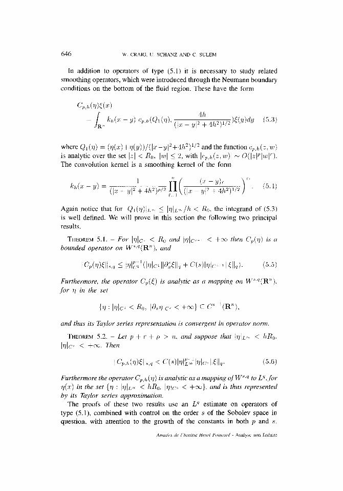
In addition to operators of type (5.1) it is necessary to study related smoothing operators, which were introduced through the Neumann boundary conditions on the bottom of the fluid region. These have the form

where Qr(v) = (r~(~~)+r~(y))/(l3.-y/2+4h2)“~ and the function ~~,~(z,wj is analytic over the set 1x1 < Ro. ITUI < 2, with Ic~~,~~(z,uI)I N O(IZIP~*UI~I’). The convolution kernel is a smoothing kernel of the form

IZ kh(Z - Y, = (I:[; - ?!I2 !t. 4fl,2)p/2 p=, (I:rI - :,,I2 + 4/,,2)1/2 n(

(.I. - Y)c >

!‘I (5.4)

Again notice that for IQr(rl)/L- < /rllL-//~ < RO, the integrand of (5.3) is well defined. We will prove in this section the following two principal results.

THEOREM 5.1. - For lrll~ < R. and Ir~lc~+ L < +x then C,(,r/) is a bounded operator on Ws.q(R1’), and

llcp(7/m,q I l7$2(lvlc~ ll;?“,Ell, + c(s)l7k-+l Ilrll,). (5.5)

Furthermore, the operator CP(<) 1s analytic as a mapping on IJV~‘.~(R’~), for 71 in the set

and thus its Taylor series representation is convergent in operator norm.

THEOREM 5.2. - Let p + 1’ + 0 > 71, and suppose that jrlL- < hR0, 17/lcs < +x. Then

Furthermore the operator Cp,h(7j) is analytic as a mapping of W”‘q to Lq, for r/(z) in the set (7 : IrllL- < hR.0, IqlcS < +oo}, and is thus represented by its Taylor series approximation.

The proofs of these two results use an L’J estimate on operators of type (5.1), combined with control on the order s of the Sobolev space in question, with attention to the growth of the constants in both p and s.


Clearly the more sensitive of the two theorems is Theorem 5.1. The form of result that we need is the following.

THEOREM 5.3. - Considerfunctions r/l(z), . . , T/~(X) E C’(RR) and k(z) a singular integral kernel satisfying the standard estimates (5.2). Then the homogeneous operator qf degree p,

qJv1 i . . . 1%)~(4 = / k(z - Y) fi Q(?iK(Y)dY (5.7) j=l

is bounded on Lq(R”), and satisfies the estimate

with exponent M = 3 + 6. The proof is fundamentally based on the following theorem of M. Christ

and J.L. JournC, [3] on Lq bounds for Calderon Zygmund commutators.

THEOREM 5.4 ([3], Theorem 4). - Consider the singular integral operator L with kernel

L(~.~~)=K(~-y)iiI(j’biiii+(l-i)li)rii). (5.9) j=l 0

where each bj E L”(R”), and K(z) satisfies the standard estimates (5.2). Then

II / L(z, YHY)dYII, 5 cc4 dGPN (fi lbb) lllllq. j=l

(5.10)

In fact one may take N = 2 + S, where 6 appears in the standard estimates (5.2), as does the constant Cl.

Proof of Theorem 5.3. - The integral kernel is

k(:r-y)fiy(7,j)=k(:I~-Y) c fifrl;I;z j=l permutations I, j=l

s

1

X &, 7)j(kE + (1 - t)y)dt (5.11) 0

Vol. 14. n” 5-1997.


since

The sum is taken over all possible L1, !2, . . . . L, between 1 and 71 (giving 71,P many terms). For each summand the result is an integral operator with a convolution kernel of the form

and whose remaining factor is

(5.12)

with b,,j(z) = &,,,rl,j(:rz). Such operators are the subject of the paper of Christ and JournC, which gives the Lq(R”) bounds.

We would like to remark that we are using K(z) = k(z)JI~=‘=,z~~ /ID:~, so that it itself depends upon the power p, and the constant Cr in the standard estimate (5.2) will be affected. This changes the ultimate power of p that appears in Theorem 5 3.

LEMMA 5.5. - If k(z) satisfies the standard estimate (5.2) with constants Cl and 0 < (5 5 1, then the kernels

sati& the standard estimates, with constants C(p) = O(pC1).

Proof. - Clearly the product does not change (5.2)(i), for we have

The estimate (5.2)(ii) is


Using this lemma and Theorem 5.4, we have essentially completed the proof of Theorem 5.3. Each of the terms in (5.11) is estimated in the L” bound of (5.9),

Since

c fi Ia.Z,z71jIL-= < fi lqJlcl

permutations I’, j=l j=l

and the constant C(p) = pCI is linear in p, we have the estimate

with M = N + 1 = 3 + 6. To continue the section we move to estimates of these singular integral

operators in higher Sobolev norms. For this we use the following lemma on the commutation of differentiation with singular integral operators E~',(71~:. .q,) defined in (5.7).

LEMMA 5.6. - Assume that k(x) is smooth away from :I: = 0, and that c$,l, . . , Q,) is a smooth function of the difference quotients Qj = Q(71,j).

&(k(x - y)cp(Q1,~ . . &,)I

= -d,(k:(x - y)c,(Q,, . . Q,))

+ k(x - y) 2 a~,~p(Ql.. Qp) Q(8.cII.j). (5.14) j=l

Proolf. - We simply check the calculation that

a Q(71-) = a.cVj(x) 71i(z) - 7/j(!/) s 3 In:-

/x _ y/I" (2: - u)

a

?f

Q(v,) = -ax%(Yl) + %cx) - %(y) ( : I : _ ?,)

J Ix - yl Ix - yl" c -


From Lemma 5.6 the commutator of operators (5.1) or (5.7) with partial derivatives is given by the expression

where 5’; is of the same form as (5.7), with integrand

(5.16)

Using Lemma 5.6 recursively, we have that

Notice that there are p”-I”- many terms in the summand, in the case that /r/-many derivatives fall on the function E(z). From Theorem 5.3 we can bound the resulting operator;

- c cd” (fi lmlc’) I18xlILY. (5.18) <

/CI+TJ=S .j=l

Standard interpolation gives that I~:~/cI 5 I~~I:‘l~‘~~/ij:r,l~!“~, thus our operator estimate becomes

Using the second interpolation that l8,“~lcl Ij8~<[/,, I ( IV[CI II8~<ll, + ~WW1l~~ll5ll~)~ for Id + m, = s, we have shown that the Ly-norm of


(5.17) is bounded, in fact we have proved the following, since there are at most @-many terms on the r.h.s. of (5.19).

THEOREM 5.7. - Suppose that 1 < q < +cc, and that rl E Cs+‘(R1’), and consider the mapping properties of the operator S,(q, . . , q). We have the estimate

Proofs of Theorems 5.1 and 5.2. - The aim is to address the general case of an integral kernel which is a general analytic function of the quotient Q(r)), in the form of the operators (5.1). Using Taylor series to describe cP( 2) = C,,, zp(c,/rrzj!).zn’ gives us the definition

(5.21)

Considered as an operator on Lq(R”), this series converges in operator norm for lqlc* 5 R < Ra. Indeed, because of estimate (5.8), the Taylor coefficients of C,(Q) grow no faster than C~Ic,,lrnnl~~~~, , which is bounded by some Crrr,!Rn’ by comparison with the Taylor series for the function &B~‘c~(z) which is also analytic on the ball IzI < Ro, of course.

This behavior is not drastically modified when considering CP(rj) on W”+Z(Rn); we work with the estimates of Theorem 5.7 to obtain

< c l&lAf+s ‘rrt,! I$7’(l4? Ilall, + wl~4c~+~ llrll,). (5.22)

rn>p

This is again seen to be convergent in operator norm, as the Taylor coefficients are again controlled by Crn!R” when 1711~1 < R < RO, by comparison with the Taylor series of the analytic function ~?‘~+~i)~‘+“c,(z) which has the same radius of convergence as cP. When we recognize that qs-4 - O(lzl”) th’ g’ is Ives the result stated in Theorem 5.1.

The remaining subject of this section is the proof of Theorem 5.2, concerning the smoothing operators Cp,h(v). These are of the form (5.3) with smoothing kernels described in (5.4). The number of factors Cy=‘=, 1’1

Vol. 14. no s-1997

652 W.CRAIG,U.SCHANZ AND CSULEM

in the product (5.4) need not grow in p. Using the analyticity of cII(z. ‘w) we can represent the smoothing operators in Taylor series,

c,., (7/)&r:) = c * .i.c

The conclusion of Theorem 5.2 will follow from an estimate in Lq(R’“) of the smoothing operators

and their derivatives. In order that the integrand be absolutely integrable, we ask that p + P + ~1 > 11.

THEOREM 5.8. - In case p + ci + y > r~ and both Irjl~- < hRo,

If%& < +oc, then the estimates hold;

Using this estimate in a manner similar to the proof of Theorem 5.1, the results of Theorem 5.2 will also follow.

Proof. - The simple LY-bounds on S,,,(v) come from the expression

Since

Ql(7) = 2h ,r/(:c) + q(y)

(Ix - y/12 + 4vy 2h %

then


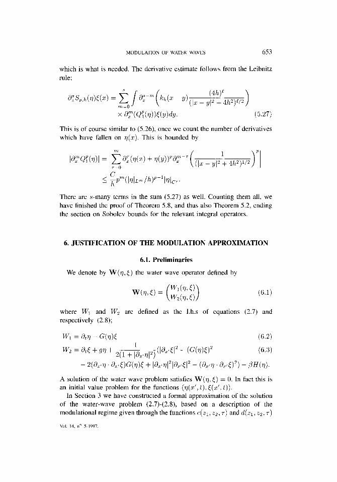
which is what is needed. The derivative estimate follows from the Leibnitz rule:

x %?Q?r(rl))E(~)d~. (5.27)

This is of course similar to (5.26), once we count the number of derivatives which have fallen on q(s). This is bounded by

There are s-many terms in the sum (5.27) as well. Counting them all, we have finished the proof of Theorem 5.8, and thus also Theorem 5.2, ending the section on Sobolev bounds for the relevant integral operators.

6. JUSTIFICATION OF THE MODULATION APPROXIMATION

6.1. Preliminaries

We denote by W(q, I) the water wave operator defined by

(6.1)

where IV1 and IV2 are defined as the 1.h.s of equations (2.7) and respectively (2.8);

WI = &I- G(rl)l (6.2) w, = a,< + gq + 2(l + I’a,,,2, wdl12 - Kw9*

A solution of the water wave problem satisfies W(r), I) = 0. In fact this is an initial value problem for the functions (r7(~‘,t),<(~‘.t)).

In Section 3 we have constructed a formal approximation of the solution of the water-wave problem (2.7)-(2.8), based on a description of the modulational regime given through the functions c( ~1: 22,~) and d( zi . z2,r)

Vol. 14, Ilo 5.1997.


which satisfy the Davey-Stewartson system (3.24). In the physical variables given by z1 = F(:L~ - w’t). x2 = F:L~, and 7 = ~‘1, the approximate solution is given by

+j = ,,/(I) + ,242) + ,:y)

[ XI fp + f2((2) + &$3), (6.4)

where (v(l). c(l)) is defined by the expressions

The formal procedure also gives the higher order components of this expression, (q(‘), [(2)) and (r](s). $“) ), which are respectively (see (3.19) and (3.25))

with coefficients (rL, rv:, n,, “(, depending on w, h:, /A, jj and ~1 and $0 = k;lZl - wt.

The basic question that we are to address in this article is the extent to which the above formal solution deviates from being a true solution of the full Euler equation description of the evolution of the free surface, given by a solution of the system W(7), [) = 0. More precisely, consider the initial condition (*Q, lo) = (,;I, F) 1 = t e, and let (71, <) be the solution of the initial value problem W(q, <) = 0 with the initial condition (71” T [a). The strongest possible result would be to compare the exact solution (,r], <) of (6.1) with the modulation approximation (v; I) in an appropriate norm, with an estimate of the form


over an interval of time 1 = [0, to] with to = O(F-~). Such a result would require an existence theory for the water wave in three space dimensions for solutions which do not develop singularities over long time intervals, given initial conditions of size O(E). This is currently an open mathematically problem, whose resolution is not given in this paper. We limit ourselves instead to presenting a weaker result, evaluating the accuracy to which the modulational solution (f, <) satisfies the water wave problem. Equivalently, we give an estimate of W(,v, F) in a Sobolev norm, and show that it is o(E~) uniformly in the time interval I. This is already a challenge, due to the singular nature of the formal derivation, in which integral operators of potential theory (with coefficients depending on multiple scales) are approximated by differential operators, and error terms contain high derivatives of the basic dependent variables.

Before we proceed with the analysis, we need to introduce some tools concerning the mathematical theory of the Davey-Stewartson system and the analysis of pseudo-differential operators with their action on multiple- scale functions. This is the object of the two following sections. Finally, in the last section (Section 6.4), we establish an estimate for W(ij, F).

6.2. The Davey-Stewartson system

In this paragraph, we recall some mathematical results for the initial value problem for the Davey-Stewartson system (3.24). After simple resealing, one can reduce the system to

ic, + &LIZ, + czzz2 = Xl& + bed,,

&,3, + rrld,2,2 = Iclf, (6.8)

with the initial condition c(zl, z2,O) = CO(Z~! ~2). The coefficients 0 and X can be normalized to be of absolute value 1. The character of the solutions depends strongly on the sign of the parameters 5 and m. Indeed, the system is classified as elliptic-elliptic, elliptic-hyperbolic, hyperbolic- elliptic and hyperbolic-hyperbolic according to the respective signs of b and m. However, the hyperbolic-hyperbolic case is not encountered in physical situations.

Boundary conditions depend on the sign of no as discussed in [l]. For rn > 0, they reduce to c --+ 0 and d 4 0 when ~1” + ~22 + cc. For rn < 0, they are of radiation type, that is, c -+ 0 when Z; + Z; + cc and d + 0 when the characteristic variables z1 f fizz 4 foe, with no condition when z1 f ~5%~ + --x.

We report below the main results concerning strong solutions. Detailed study of strong and weak solutions, together with long time behavior can be found in [13], [14], [16] and [20] and [26].

Vol. 14, Ilo 5.1997.


THEOREM 6.1. - Suppose rr/, > 0. Given an initial condition c0 in H”(R2), there exists a unique solution (c. d) during a jinite interval of time [O, rl) such that c E C([O, T-I), H”(R2)) and d E C([O, ~1). H’+l(R2)).

In the elliptic-elliptic case, the situation is similar to that of the cubic Schrijdinger equation: if X > ma:r:( -h, 0), smooth solutions can be extended for all time, while if X < ma:r:( -b, O), solutions may focus in a finite time [13]. The structure of the singular solutions is critical as in the two- dimensional cubic SchrBdinger equation [24]. In the hyperbolic-elliptic case, smooth solutions can be extended for all time if the L”-norm of the initial conditions is small enough [ 131.

The elliptic-hyperbolic and hyperbolic-hyperbolic cases are more complex. Existence of smooth solutions has been proved first by Linareh and Ponce for small initial data in weighted Sobolev spaces [20]. In ;I recent work, Hayashi and Saut [16] proved local existence of sulutions in some analytic function spaces without a smallness condition on data. They also proved global existence of small solutions. We state below a recent result by GuzmAn-G6mez [ 141 in usual Sobolev spaces that gives a bound on the L2-norm of the initial condition to ensure local existence.

THEOREM 6.2. - Suppose S > 0 and 711 < 0. For initial condition co E H3(R2) satisfying Ico~$ < e, there exists a unique solution (c, d) during a finite interval of time [O: ~22) with c E C([O, TZ), H”(R2)) and d E C([O, 72), W2+(R2)).

6.3. Multiple scales and pseudo-differential operators

We first define the analytic framework in which we will work. Consider a function u(z’, z’), with Z’ E R” and Z’ E T” = RyL/I’, where l? is the lattice with respect to which u is periodic in IC’. For 2’ E R” and 0 < t, we define a multiple scale function as a function u(:c’, z’), evaluated on the subspace {z’ = FX’} C R2”. We will use the notation ~(2’. ~2’) or u(x’, z’)(,,,,,, for such functions. For functions u = u(x’) (which may depend upon t as well), the usual Sobolev W”,q-norm is written IIu(I~.~. When a multiple scale function c depends upon the slow variables alone, that is, c = c(Fx’), it is measured in a Sobolev norm in that variable,

I&y = c,,,,<, (.I’ li);“.r:Iq’q. Scaling by f provides a relationship

between these two norms; [Ic/~,,~ 5 t-“‘Y[~l,,~ for any F < 1. For the expected modulational form of approximate solutions to the water wave problem, a third norm is used for estimating multiple scale functions. For


u = u(x’; a’), we define

The analysis of the modulational regime of the water wave problem involves classes of functions of the form u(x’, z’)[~,=~~~ = ~xp(‘I:~s’)c(~‘)~~‘=~~,, for z’ E R2, and the above discussion implies that

A norm related to (6.9) is used in [SJ for the analysis of pseudo-differential operators and their actions on multiple scale functions. Here we give an analogous result on the bounds for pseudo-differential operators, using the IV”14 norms as our reference point.

A Fourier multiplier operator is defined as

(6.10)

where ?I is the Fourier transform m of U. For u a multiple scale function of :I:’ E T” > z’ E R”, M(D)u depends upon E and z’, but is not in general a multiple scale function, However it does have an asymptotic expansion in terms of them.

THEOREM 6.3. -Assume that the Fourier multiplier M(D) has the property that l@h/l(lc)l < cj(l + 1k12)(m-j)/2, 0 5 j < m. Then its operation on a multiple scale function has an asymptotic expansion

+ RN+IU . (6.11)

The remainder has the estimate

where the subscripts are &I = m - (N + 1) + s + (T, !, = s + 0 + max(rrL, N + 1) for any (T > 71.

Given the analysis of reference [8], the proof of this result is relatively standard. For sake of completeness however, we give it in Appendix B.

Vol. 14, Ilo s-1997.

658 W.CRAIG. U. SCHANZ AND C. SULEM

6.4. Estimates on the water-wave operator acting on the modulational approximation

As noted before, the character of the solutions of the Davey-Stewartson system is different whether the equation for (i is of elliptic (7~ > 0) or hyperbolic type (sn < 0). Thus, we will divide the analysis into these two cases referred to as case I and case II respectively.

In case I, starting with an initial condition co E H”(R’), there exists a unique solution (c, d), with c’ and d being continuous functions of 7- E [O; ~~1 with values in H”(R”) and H”+l (R2) (TV may be finite or infinite) and by Sobolev embedding in T/I/“,” and lV’-‘-q for s = I’ - $($ - f). From this solution, we construct a functional of the modulation approximation Gj = q( c, d) and c = f( I:. IQ using the expressions (6.4-7) in the time interval I = [0,C2 ~~1. We will establish an upper bound for W(;i, r) in the interval I in a Sobolev norm in terms of powers of c and Sobolev norms of c and d.

In case II, we start again with an initial condition in H“(R2). There exists a unique solution (c. d) with c being continuous function of 7 in [0, ~11 with values in H’(R2) and thus in IV’.q(R2) and tl a continuous function of T with values only in Ws-l.r and thus not integrable. To overcome this difficulty, we introduce a cut-off function )i infinitely differentiable with compact support and we construct q = ,;T(c. u/i) and < = C(C. x(i). An upper bound will be established for W(sq, 0.

In both cases, an important point is the amount of derivative loss. To quantify these amounts. we introduce the notion of estimating factors which are functions F(sl. s2) that are non-negative, continuous, and satisfy F(O,O) = 0, with polynomial growth in (s, . s2), (and depending on li: and w).

LEMMA 6.4. - Set ;i and < as in (6.4-7), the approximations to the operator G(r/) of Section 4 sati;fi


Proof. - An application of Theorem 4.7 gives:

IIwiEllw 2 m$m7lc~ IIFlls+l,q + C(.s)l71b+1 Il~lLq, (6.16)

for j = 1,2,3. We have furthermore from the approximate solutions and Gagliardo-Nirenberg inequalities:

IIFI s+l,q 5 ‘F’(w$ IcIc~)(ll4s+2,~ + Il4s+l,,) (6.17)

lfjllc”+l i FF2(SUP IcIcs+3, sup ldlcs+2). (6.18) tEI tEI

THEOREM 6.5. - Consider the case m > 0. Let (c, d) be a solu$on of the Davey-Stewartson system (3.24). The approximate solution (;i, [)(c, d) satisfies the estimate:

;l$ IIWK m,q

< ~~-~‘~F(sup I&“+. - 37 ;iF ldlcs+2)(ICls+6,q + Idls+6,q) (6.19) tcI

Proof. - We start with

We have shown that the last term can be estimated by

IIR3eiIkl

I ~4F(s~~ lclc tEI s+3> 27 IdIc~+4II4+z,q + Ildlls+d

5 ~“-~‘~F(sup I+“+. tcI we I4c~+4(I4~+2,q + l&+l,q) (6.21)

Since we consider the expression as a multiple scale function, we replace i& by i% - cw’d,, + t2& . The computation of &t;i is similar to the one performed in [8 , eq.(5.7)]. We obtain an expression at order c3 with a remainder of the form

R4 = ~4(-w’dz,~(3) + a~+~)) + ~~d,q(~). (6.22)

Using the expressions of ~(~1 and ~(~1 in terms of c and d given in (6.6) and (6.7) and the fact that, when m > 0, we have the estimate [13]

IPd4lq 5 cIIIc1211q: Vol. 14. no 5.1997.


the IV’14 norm of R4 is bounded by

Next, we use the multiple scale approximations for the integral operators (GO + Gr (q) + G2(r7))c When applied to $l), we expand GO up to order c2:

GoJ(l) = &lmeiy - if2 (D + I& (1 - CT”)) c,, eiip

- c3 (( 2 + $1 - cT2))c,,,2 + (h(l - CT”) - h%~a(l - 2))c,,,, e&Y + c. c

> - f3qL,z, + dz2z2) + R4 (6.23)

A direct application of Theorem 6.3 gives

11R411s,n 5 cF4(IIcIIs+6,q + 1k%+6,,)

When applied to E~J(~) (resp. e3t(“)), we expand GO to order E (resp. zeroth order). We next address G,(;il).$ We recall that

G1 (if)? = D . ;ijDf - GoiJGof. (6.24)

To expand G1(5j)l, we first write

D . ;rDc= (Dp) + cD$‘))sj(D~) + ED!‘))?+ e2D;%jD;)F. (6.25)

Substituting ?j and c by their expressions (6.4), D . tjDf has an expansion in c up to order three and a remainder R4 bounded in W’%q-norm by:

“4F’“,FT l”l“>;~p I4c4(114+3,q + lldlls+2,q).

For the second term of G1, we use Theorem 4.2 of [8] on composition of operators and get:

Go;;ico& -,2G(0)rl(l)G(O)((1) _ t3 ($O)rl@)G(0)((l)

+ ($0)77(1)G(0)$2) + ($o)rl(l) ( tanh(/@))Dil)

+ hDiO)(l - tanh’(hDIO’))Dl”)~(‘) + ( tanh(hDp))D$l)

+ hDp) (1 - tanh2(hDy))) D~l))r/(l)G(o)<(l)) +R4. (6.26)


Again, the remainder R* is bounded in W”‘J-norm by

A similar computation is done for Gz(?j)c Combining all these results,it follows that, by the construction of Section 3, in the expansion of WI@, 0, the terms up to order e3 cancel and the remainder has a Ws’4-norm bounded from above by the r.h.s of (6.19).

The same computation (although a little heavier) is performed for Wz(?j, F). This completes the proof of Theorem 6.5 devoted to the case m > 0. We turn ‘now to the case m < 0.

As mentioned before, the function d is in lVs+(R2) without being in any q-integrable spaces. This is due to the hyperbolic nature of the second equation of the Davey-Stewartson system. In this case, we have a local result. Let x(2’) E Cr ( R2) a cutoff function such that ~(2’) = 1 for [?‘I < R. Consider the approximate solutions ?j = ?j(c, xd) and c = [(c, xd), where (c, d) satisfies the Davey-Stewartson system.

THEOREM 6.6. - Let (c, d) solve the Davey-Stewartson system in the case m < 0. The truncated approximate solution (fj [) satisfies the estimate:

;:‘l Ilx1wvL IIls,q

-=c F~-~‘~F(su~ I& - s+3r “,Ey ldb+d(kds+6,q + /X&+6,,) (6.27) tEI

for aEl x1 E Cr(R2) with supp(xl) C: BR(0).

Proof. - It follows the steps of the proof of Theorem 6.5: Again, we separate G(q) in the form

G(v) = (Go + G(ii) + G2(rl)) + R3(71)

and apply Lemma 6.4 to estimate the remainder. When computing W(fl, I), we use the multiple scale approximations and get that W(q, c) is equal to a functional of the Davey-Stewartson operator applied to (c, xd) plus a remainder of the order of O(E~). When the support of x1 is included in a set on which xd = d, xi W(?j, [) reduces to a remainder of order O(e4). A localized version of the same conclusion then follows.

Vol. 14, Ilo 5-1997

662 W.CRAIG, U. SCHANZ AND C. SULEM

ACKNOWLEDGEMENTS

The work of the first author was partially supported by the National Science Fundation grant DMS-9401377 during the time that this research was performed, and the work of the third author by NSERC operating grant OGPINI 6.

APPENDIX A

This appendix is devoted to the computation of the Fourier transforms of various kernels arising in the derivation of the Taylor expansion of G. Let F denote the Fourier transform. In the following, k E R2 will be the variable in the Fourier space and x E R2 the variable in the physical space.

PROWSITION A.1

COROLLARY A.1

3 (1x12 +&’ >

= ~2~T&$e-‘“l”l (j = 1,2)

COROLLARY A.2

3 ( 1

& = -2Tlk

3 (

(IcE,2 t2h;h2)3,2 = 27re-2h,‘“’ >

3 24h”

([xl2 + 4h2)5/2 > = 27r( 1 + 2hlkl)e-2h’k’

COROLLARY A.3

3 16h5

( )cc12 + 4h2)7/2 &l + 2h(k() + ;h’[k[‘),‘““1

(A.11

(A.2)

(A.3)

(A.41

(A.5)

(AX)

(A.71

(A.81

(A.91


Let us first obtain the Corollaries from proposition A.l:

ProofofCoro2Zm-y A. 1. - Equality (A.2) is obtained from (A.l) by taking the limit h -+ 0. Equality (A.3) is obtained from (A.l) by differentiation and (A.4) as the limit of (A.3) when h -+ 0.

Proof of Corollary A.2. - To get (AS), we notice that I = -A 1x13

and to get (A.6) we rewrite (A.l) as

(Ix12 +l;lh2)3,2 = &&e-2h’k” >

Finally, (A.7) is obtained from the identity

A ( [xl2 +:h2)‘i2 = > ([xl" +:bZ)3/2 -

12h2 ([xl” + 4h2)5/2.

and (A.l) and (A.6).

Proof of Corollary A.3. - Equality (A.@ is a direct consequence of (A.6)

and (A.9) results from the computation of A ( (1x1” +ih2j3i2 ’ >

Proof of Proposition A.1. - Let us compute 3-l (A,-WI):

After some elementary computations, we get

1 1x1” cos2 $0 + 4h2 dv

Using the change of variable 8 = tancp, we get

3-1 ( he-2h’k’) = & (lx12 +:h2)1,2

Vol. 14, Ilo 5-1997.


APPENDIX B

This appendix is devoted to the proof of Theorem 6.3. The Fourier multiplier operator M(D) is defined as

and has the property that l8Fm(<)l 5 cj(l + 1<]2)(‘rL--/(yl)/2, 0 2 n < m. Let U(Z, EZ) = U(Z, z)Izztz be a multiple scale function with IC E T” and z E R”. When applied to U(Z, EX) Fourier multipliers have the asymptotic expansion in multiscale functions

(M(D)u) (CT; E) = (2 $3$qD,)(-ia,)iu) (cc, EZ)+RN+lu (B.2) J=o .

(see eq (4.8) of ref. [8] for details), with the remainder term RN+~u given by

(J

1 N La”+’

o N! c rn(< + dr))f&

> D,N+l u(z’, z’)da’dz’d(d~. (B.3)

The order of 8:” m(.) is m - (N + 1). To estimate RN+~u, we separate the domain of spatial integration in four parts:

(i) IIC - 5’1 > l/2 and IEZ - z’] > l/2, (ii) 1~ - 2’1 5 3/2 and IEZ - z’] < 3/2,

(iii) 12 - z’l > l/2 and IFD: - z’l 5 3/2, (iv) 1~ - z’/ < 3/2 and ICC - z’l > l/2,

focussing on the individual regions using a smooth partition of unity {x(~)(x, x’, z’)} adapted to this decomposition. We denote by Rg’+lu, Rcii) N+lu . . . their corresponding contribution to RN+~u.

Over the first region, the contribution to the error term is

x Ly+5L(z’, z’)p(~, d, z’)drc’dz’d<dq. (8.4)

Anna/es de I’lmtrtut Henri Poincnrh Analyse non lindaire


We estimate the oscillatory integrand to be

pp;a;+l m(( + +)I < c,(d)7(1 + I< + drj12)m-(N++2T

Now, we separate the contributions 171 < 31[1/2 and 1~1 > Ill/a, with similar smooth cutoff functions j$l)(<, q), J$~)(<, 7). When 1~1 < 31[1/2, the oscillatory integral is absolutely convergent as soon as y > (m - (N + 1))/2 + n/2. Furthermore, the integrand

is integrable in (x’, z’), uniformly in 5, and is also integrable in z, uniformly over (x’, 2’). Note that no additional derivatives act on the function U.

When Iv1 > IlIP we rewrite the contribution in the form

x (1 + I[I”)-“““(l f lr$)-62’2

x (1 - a,pq 1 - a,+Q’“D,N+‘u(S’, z’)dx’dz’d@7& (B.5)

To have an absolute convergent integral, we choose S1 > n and & > n. This places & derivatives with respect to x’ and N + 1 + S2 derivatives with respect to z’ on U.

Now we turn to Rcii) N+l~, paying less heed than we should to the smoothness of U. We rewrite it in a form where all derivatives act on u(2’, 2’):

R@) N+l

‘LL = p+1 J ei(E+t17)"e-i(E1'+172))(1 + 1<12)-‘l/2(1 + J11)2)-7z/2

(/

1 N

X Li)“+l

*(J N! E m([ + ct~)dt

>

(1 - n,r)6q1 - .*p2p+1 z u(2’, z’)dz’dz’d<d~. (B.6)

Notice that the spatial domain is uniformly finite in z for each (x’, z’). Choosing yl,y2 > n + m - (A’ + l), the oscillatory integrals are absolutely convergent. In this term, we have at most n + rn - (N + 1) derivatives

Vol. 14, no 5-1997.


with respect to z’ and n, + m - (N + 1) + (N + 1) derivatives with respect to z’ on u.

We rewrite RE?ru. as

R(G) N+l

u = p+1

.I

x D,N+lu(x’, .z’)dx’dz’d<dr/ (B.7)

Here we separate the contributions where jr/l < 31<1/2 and 1711 > ]4/2 and proceed as in case (i). We thus choose y > n and y > m - (N + 1). The count of derivatives gives at least n + m - (N + 1) derivatives with respect to x’ and n + (N + 1) derivatives with respect to z’ on U.

The last term to estimate is R$“‘,u.

x Dc’T+lu(x’, z’)dx’dz’d<dq

Take y > n and y > m - (N + 1). Then, i3;li8ri+‘m will be bounded and the power y of l/l EX - ~‘17 will be integrable in z’, uniformly over IC. Note that for given 5, z’ varies over a uniformly bounded cube. Furthermore, for fixed (x’, z’), the z-integral also varies over a uniformly bounded cube. To bound the oscillatory integral, we separate the contributions where 14 < 3lElP and Iv > IlIP g a ain by smooth cutoff functions. When InI < [<l/2, we choose y > ‘IL. When 171 > Icl/2, we follow the procedure above and write this contribution as:

x (1 + 1<~2)-“‘“(1 + )7/12)-y”‘2 (1 _ &)d2(1 _ Az,)~~/2~“+1 2 ~(2’. z’)dx’dz’dfdq. (B.9)

Here we choose yl, y2 > r~ and we have the same count as case (iii) above. This completes the proof of Theorem 6.3.


REFERENCES

[I] M. J. ABLOWITZ and H. SEGUR, J. Fluid Mech., Vol. 92, 1979, pp. 691-715. [2] D. J. BENNEY and G. .J. ROSKES, Stud. Appl. Math., Vol. 48, 1969, pp. 377-385. [3] M. CHRIST and J. L. JOURN& Am Math., Vol. 159, 1987, pp. 51-80. [4] R. R. COIFMAN and Y. MEYER, Proc. Symp. Pure Math., Vol. 43, 1985, pp. 71-78. [5] P. COLLET and J. P. ECKMANN, Comm. Math. Phys., Vol. 132, 1990, pp. 139-153. [6] W. CRAIG, Comm. Part. DifJ: Eq., Vol. 10, 1985, pp. 787-1003. [7] W. CRAIG and M. GROVES, Wave Motion, Vol. 19, 1994, pp. 367-389. [8] W. CRAIG, C. SULEM and P. L. SULEM, Nonlinearity, Vol. 108, 1992, pp. 497-522. [9] W. CRAIG and C. SULEM, J. Camp. Phys., Vol. 108, 1993, pp. 73-83.

[ 1 O] A. DAVEY and K. STEWARTSON, Proc. Roy. Sot. A, Vol. 338, 1974, pp. 101-l 10. [l 1) V. D. DJORDJEVIC and L. G. REDEKOPP, J. Fluid Mech., Vol. 79, 1977, pp. 703-714. [12] P. R. GARABEDIAN and M. SCHIFFER, J. Analyse Math&zatique, Vol. 2, 1952, pp. 281-368. [13] J. M. GHIDALIA and J. C. SAUT, Nonlinearity, Vol. 3, 1990, pp. 475-506. 1141 M. GUZMAN-G~MEZ, PhD thesis, University of Toronto, 1995. [ 151 H. HASIMOTO and H. ONO, J. Phys. Sot. Japan, Vol. 33, 1972, pp. 805-811. [16] N. HAYASHI and J. C. SAUT, D# and Integral Equations, Vol. 8, 1995, pp. 1657-1675. [ 171 T. KANO and T. NISHIDA, J. Marh Kyoro Univ., Vol. 19, 1979, pp. 335-370. [18] T. KANO and T. NISHIDA, Osaka J. M&h., Vol. 23, 1986, pp. 389-413. [ 191 P. KIRRMANN, G. SCHNEIDER and A. MIELKE, Proceedings of the Royal Society of Edinburgh,

Vol. 122A, 1992, pp. 85-91. 1201 F. LINARES and G. PONCE, Ann. Inst. PoincarP, Analyse nonlin&ire, Vol. 10, 1993,

pp. 523-548. [21] R. de la LLAVE and P. PANAYOTAROS, Water waves on the surface of the sphere, J. Nonlinear

Science, Vol. 6, No. 2, 1996, pp. 147-167. [22] A. NEWELL, Solitons in Mathematics and Physics, SIAM, Philadelphia, 1985. 1231 L. F. MCGOLDRICK, J. Fluid. Mech., Vol. 52, 1972, pp. 725-75 I. [24] G. C. PAPANICOLAOU, C. SULEM, P. L. SULEM and X. P. WANG, Physica D, Vol. 72, 1994,

pp. 61-86. 1251 R. PIERCE and E. WAYNE, On the validity of mean-field amplitude equations for counter-

propagating wavetrains, Nonlinearity, Vol. 8, No. 5, 1995, pp. 769-779. [26] M. TSUTSUMI, J. Marh. Anal. Appl., Vol. 82, 1994, pp. 680-704. 1271 V. E. ZAKHAROV, J. Appl. Mech. Tech. Phys., Vol. 9, 1968, pp. 190-194.

(Manuscript received September 27, 1995; revised April 30, 1996.)

Vol. 14. Ilo 5-1997.

the modulational regime of three-dimensional water waves and the davey-stewartson system

Documents