NBER WORKING PAPER SERIES

THE MINIMUM WAGE AND THE GREAT RECESSION: EVIDENCE OF EFFECTS ON THE EMPLOYMENT AND INCOME TRAJECTORIES OF LOW-SKILLED WORKERS

Jeffrey ClemensMichael Wither

Working Paper 20724http://www.nber.org/papers/w20724

NATIONAL BUREAU OF ECONOMIC RESEARCH1050 Massachusetts Avenue

Cambridge, MA 02138December 2014

We thank Jean Roth for greatly easing the navigation and analysis of SIPP data, as made accessiblethrough NBER. We thank Prashant Bharadwaj, Julie Cullen, Gordon Dahl, Roger Gordon, Jim Hamilton,Karthik Muralidharan, Johannes Wieland, and seminar participants at Brown, Cornell-PAM, TexasA&M, and the 2014 Young Economists Jamboree at Duke University for helpful comments and suggestions.We also thank the University of California at San Diego for grant funding through the General CampusSubcommittee on Research. The views expressed herein are those of the authors and do not necessarilyreflect the views of the National Bureau of Economic Research.

At least one co-author has disclosed a financial relationship of potential relevance for this research.Further information is available online at http://www.nber.org/papers/w20724.ack

NBER working papers are circulated for discussion and comment purposes. They have not been peer-reviewed or been subject to the review by the NBER Board of Directors that accompanies officialNBER publications.

© 2014 by Jeffrey Clemens and Michael Wither. All rights reserved. Short sections of text, not toexceed two paragraphs, may be quoted without explicit permission provided that full credit, including© notice, is given to the source.

The Minimum Wage and the Great Recession: Evidence of Effects on the Employment andIncome Trajectories of Low-Skilled WorkersJeffrey Clemens and Michael WitherNBER Working Paper No. 20724December 2014JEL No. I38,J08,J21,J38

ABSTRACT

We estimate the minimum wage's effects on low-skilled workers' employment and income trajectories.Our approach exploits two dimensions of the data we analyze. First, we compare workers in statesthat were bound by recent increases in the federal minimum wage to workers in states that were not.Second, we use 12 months of baseline data to divide low-skilled workers into a "target" group, whosebaseline wage rates were directly affected, and a "within-state control" group with slightly higher baselinewage rates. Over three subsequent years, we find that binding minimum wage increases had significant,negative effects on the employment and income growth of targeted workers. Lost income reflectscontributions from employment declines, increased probabilities of working without pay (i.e., an"internship" effect), and lost wage growth associated with reductions in experience accumulation.Methodologically, we show that our approach identifies targeted workers more precisely than thedemographic and industrial proxies used regularly in the literature. Additionally, because we identifytargeted workers on a population-wide basis, our approach is relatively well suited for extrapolatingto estimates of the minimum wage's effects on aggregate employment. Over the late 2000s, the averageeffective minimum wage rose by 30 percent across the United States. We estimate that these minimumwage increases reduced the national employment-to-population ratio by 0.7 percentage point.

Jeffrey ClemensDepartment of EconomicsUniversity of California, San Diego9500 Gilman Drive #0508La Jolla, CA 92093and NBERjeffclemens@ucsd.edu

Michael WitherUniversity of California, San Diego, Department of9500 Gilman Drive #0508La Jolla, CA 92093-0508mwither@ucsd.edu

Between July 23, 2007, and July 24, 2009, the federal minimum wage rose from $5.15

to $7.25 per hour. Over a similar time period, the employment-to-population ratio de-

clined by 4 percentage points among adults aged 25 to 54 and by 8 percentage points

among those aged 15 to 24. Both ratios remain well below their pre-recession peaks. The

empirical literature is quite far from consensus, however, regarding the minimum wage’s

potential contribution to these employment changes (Card and Krueger, 1995; Neumark

and Wascher, 2008; Dube, Lester, and Reich, 2010; Neumark, Salas, and Wascher, 2013;

Meer and West, 2013). In this paper, we analyze the minimum wage’s effects on the

employment and income trajectories of low-skilled workers during the Great Recession

and subsequent recovery.

Our analysis harnesses the fact that the 2007 through 2009 increases in the federal

minimum wage were differentially binding across states. Between December 2007 and

July 2009, the effective minimum wage rose by $1.31 in the states we designate as

“bound” and by $0.43 in the states we designate as “unbound.” Of the $0.88 differ-

ential, $0.58 took effect on July 24, 2009. We analyze the effects of these differentially

binding minimum wage increases using monthly, individual-level panel data from the

2008 panel of the Survey of Income and Program Participation (SIPP). The SIPP allows

us to use 12 months of individual-level wage data, from August 2008 through July 2009,

to further divide low-skilled individuals into those whose wages were directly targeted

by the new federal minimum and those whose wages were moderately above. These rich

baseline data yield a number of advantages over the literature’s standard approaches.1

1Analyses of individual-level panel data are not as common in the minimum wage literature as onemight expect. Examples include Currie and Fallick (1996), who analyze teenage employment in the 1979

National Longitudinal Survey of Youth, Neumark, Schweitzer, and Wascher (2004) and Neumark andWascher (2002), who use the short panels made possible by the matched monthly outgoing rotation filesof the Current Population Survey (CPS), and Linneman (1982), who analyzed the minimum wage using1973-1975 data from the Panel Study of Income Dynamics. Burkhauser, Couch, and Wittenburg (2000)analyze the minimum wage using the 1990 SIPP, but adopt the conventional state-panel approach ofanalyzing its effects on the employment of low-wage demographic groups rather than isolating samplesof targeted individuals on the basis of baseline wage data.

1

Our approach’s first advantage is its capacity to describe the minimum wage’s effects

on a broad population of targeted workers. Past work focuses primarily on the mini-

mum wage’s effects on particular demographic groups, such as teenagers (Card, 1992a,b;

Currie and Fallick, 1996), and/or specific industries, like food service and retail (Katz

and Krueger, 1992; Card and Krueger, 1994; Kim and Taylor, 1995; Dube, Lester, and

Reich, 2010; Addison, Blackburn, and Cotti, 2013; Giuliano, 2013). While minimum and

sub-minimum wage workers are disproportionately represented among these groups,

both are selected snapshots of the relevant population. Furthermore, it is primarily low-

skilled adults, rather than teenage dependents, who are the intended beneficiaries of

anti-poverty efforts (Burkhauser and Sabia, 2007; Sabia and Burkhauser, 2010). Assess-

ing the minimum wage from an anti-poverty perspective thus requires characterizing its

effects on the broader population of low-skilled workers, which we are able to do.2

Econometrically, our setting has several advantages. One benefit of our rich baseline

data is that they allow us to limit the extent to which our “target” group contains unaf-

fected individuals. Second, the data allow us to identify relatively low-skilled workers

whose wage distributions were not directly bound by the new federal minimum. We use

these workers’ employment trajectories to construct a set of within-state counterfactuals.

The experience of these workers allows us to control for the form of time varying, state-

specific shocks that are a source of contention in the recent literature (Dube, Lester, and

Reich, 2010; Meer and West, 2013; Allegretto, Dube, Reich, and Zipperer, 2013). Third,

2Linneman (1982) similarly discusses this benefit of analyzing individual-level panel data in the con-text of minimum wage increases during the 1970s. A drawback of the individual-panel approach is thatthe resulting samples of targeted workers exclude individuals who were not employed when baseline datawere collected. It is best suited for estimating the effects of minimum wage increases on the employmenttrajectories of those directly targeted. An advantage of this study’s analysis of monthly panel data is thatour estimates capture the minimum wage’s effects on both the regularly employed and on highly marginallabor force participants. Specifically, the only individuals we are unable classify on the basis of baselinewages are those who were unemployed for all 12 baseline months. Additionally, although we do nothave a reported wage for such individuals, we can directly estimate the effect of binding minimum wageincreases on this group’s subsequent employment; the estimated effect is negative, economically small,and statistically indistinguishable from 0.

2

our research design allows for transparent, graphical presentations of the employment

and income trajectories underlying our regression estimates.

We begin by assessing the extent to which minimum wage increases affected the

wage distributions of low-skilled workers. Among workers with average baseline wages

less than $7.50, the probability of reporting a wage between $5.15 and $7.25 declined

substantially. We find that the wage distributions of low-skilled workers in bound and

unbound states fully converge along this dimension. Further, we estimate that the min-

imum wage’s bite on our target group’s wage distribution is nearly twice its bite for a

comparison sample of food service workers and teenagers.

We next estimate the minimum wage’s effects on employment. We find that increases

in the minimum wage significantly reduced the employment of low-skilled workers.

By the second year following the $7.25 minimum’s implementation, we estimate that

targeted workers’ employment rates had fallen by 6 percentage points (8 percent) more

in bound states than in unbound states.

We further analyze a sample of teenagers and food service workers to compare our

approach with approaches commonly used in the literature. For this sample, we estimate

an employment decline of just under 4 percentage points. The estimated employment

effects thus scale roughly in proportion to the minimum wage’s bite on these groups’

wage distributions. All else equal, Sabia, Burkhauser, and Hansen (2012) note that esti-

mates of the minimum wage’s effects on employment will scale with the extent to which

an analysis sample contains unaffected workers. Their insight thus points to a partial

line of reconciliation between the disemployment effects we observe and the statistical

null results found in some of the recent literature. The magnitude of our estimated em-

ployment effects also likely reflects the setting we analyze, namely the Great Recession

and subsequently sluggish recovery.

The primary threat to our estimation framework is the possibility that low-skilled

3

workers in the bound and unbound states were differentially affected by the Great Re-

cession. We show graphically that the housing crisis was more severe in unbound states,

potentially biasing our estimates towards zero. In our baseline specification, we control

directly for a proxy for the severity of the crisis. As noted above, our use of monthly,

individual-level panel data enables us to more systematically construct within-state con-

trol groups with baseline wages only moderately higher than the new federal minimum.

Our initial results are robust to netting out changes in the employment of these slightly

higher skilled workers. We further find our estimates to be robust to a broad range of

potentially relevant changes to our baseline specification.

In addition to reducing employment, we find that binding minimum wage increases

increased the likelihood that targeted individuals work without pay (by 2 percentage

points or 12 percent). This novel effect is concentrated among individuals with at least

some college education. We take this as suggestive that such workers’ entry level jobs

are relatively readily posted as internships. For low-skilled, low-education workers, the

entire change in the probability of having no earnings comes through unemployment.

We next estimate the effects of binding minimum wage increases on low-skilled work-

ers’ incomes and income trajectories. Our data provide a unique opportunity to inves-

tigate such effects, as the SIPP’s monthly, individual-level panel extends for 3 years

following the July 2009 increase in the federal minimum. To the best of our knowl-

edge, this enables us to provide the first direct estimates of the minimum wage’s effects

on medium-run economic mobility. Given longstanding and widespread concern over

developments in inequality (Katz and Murphy, 1992; Autor, Katz, and Kearney, 2008;

Kopczuk, Saez, and Song, 2010), such effects may be of significant interest.

We find that this period’s binding minimum wage increases reduced low-skilled in-

dividuals’ average monthly incomes. Relative to low-skilled workers in unbound states,

targeted workers’ average incomes fell by $100 over the first year and by an additional

4

$50 over the following 2 years. While surprising at first glance, we show that the short-

run estimate follows directly from our estimated effects on employment and the likeli-

hood of working without pay. The medium-run estimate reflects additional contributions

from lost wage growth associated with lost experience. Because most minimum wage

workers are on the steep portion of the wage-experience profile (Murphy and Welch,

1990; Smith and Vavrichek, 1992), this effect can be substantial. We directly estimate,

for example, that targeted workers experienced a 5 percentage point decline in their

medium-run probability of reaching earnings greater than $1500 per month.3 Like pre-

vious results, these estimates are robust to netting out the experience of workers with

average baseline wages just above the new federal minimum. As in Kahn (2010) and

Oreopoulos, von Wachter, and Heisz’s (2012) analyses of the effects of graduating dur-

ing recessions, we thus find that early-career opportunities have persistent effects.

After presenting these results, we compare our estimates of the minimum wage’s

effects with results from research on the effects of the Earned Income Tax Credit (EITC),

an alternative policy for increasing the incomes of low-skilled workers. The EITC has

been found to significantly increase the employment and incomes of low-skilled workers

(Eissa and Liebman, 1996; Meyer and Rosenbaum, 2001; Eissa and Hoynes, 2006), reduce

inequality (Liebman, 1998), and reduce tax-inclusive measures of poverty (Hoynes, Page,

and Stevens, 2006). The results thus contrast rather sharply.

We conclude by assessing our estimates’ implications for the effects of this period’s

minimum wage increases on aggregate employment. Over the late 2000s, the average

effective minimum wage rose by nearly 30 percent across the United States. Our best

estimate is that these minimum wage increases reduced the employment-to-population

ratio of working-age adults by 0.7 percentage point. This accounts for 14 percent of the

3Earning $1500 would require working full time (40 hours per week for 4.33 weeks per month) at awage of $8.80. We characterize $1500 as a “lower middle class” earnings threshold.

5

total decline over the relevant time period.

1 The Minimum Wage’s Potential Effects

This section briefly motivates the outcomes on which we focus our empirical anal-

ysis.4 The minimum wage can affect firm operations and workers’ well-being through

many channels. Following is a non-exhaustive list of potential margins of interest:

1. Wages of low-skilled workers.

2. Employment of low-skilled workers.

3. Income of low-skilled workers.

4. Income trajectories of low-skilled workers.

5. Firm offerings of benefits including health insurance.

6. Firm spending on the quality of workplace conditions.

7. Firm substitution between low-skilled labor, high-skilled labor, and capital.

8. Firm utilization of inputs with which low-skilled labor is complementary.

9. Incomes of firm owners.

10. Prices of goods produced by firms that employ minimum wage workers.

The list highlights the potential complementarity of firm-, industry-, and individual-

level analyses of the minimum wage. Our analysis of individual-level panel data speaks

to the minimum wage’s most direct effects on its targeted beneficiaries. These include

4Because the relevant theoretical insights have been made in a literature extending from Stigler (1946)through Gramlich (1976) to Lee and Saez (2012), we do not intend to break new ground.

6

its intended and unintended effects on the wage distributions, employment, income,

and income trajectories of low-skilled workers. Firm- and industry-level analyses may

best speak to outcomes related to the quality of workplace conditions, the utilization of

inputs that complement or substitute for low-skilled labor, the incomes of firm owners,

and output prices.

2 Background on the Late 2000s Increases in the Federal

Minimum Wage

We estimate the minimum wage’s effects on employment and income trajectories

using variation driven by federally mandated increases in the minimum wage rates ap-

plicable across the U.S. states. On May 25, 2007, Congress legislated a series of minimum

wage increases through the ”U.S. Troop Readiness, Veterans’ Care, Katrina Recovery, and

Iraq Accountability Appropriations Act.” Increases went into effect on July 24th of 2007,

2008, and 2009. In July 2007, the federal minimum rose from $5.15 to $5.85; in July 2008

it rose to $6.55, and in July 2009 it rose to $7.25.

Figure 1 shows our division of states into those that were and were not bound by

changes in the federal minimum wage. We base this designation on whether a state’s

January 2008 minimum was below $6.55, rendering it partially bound by the July 2008

increase and fully bound by the July 2009 increase. Using Bureau of Labor Statistics

(BLS) data on states’ prevailing minimum wage rates, we designate 27 states as fitting

this description.

Figure 2 shows the time paths of the average effective minimum wages in the states

to which we do and do not apply our “bound” designation. Two characteristics of the

paths of the minimum wage rates in unbound states are worth noting. First, their aver-

age minimum wage exceeded the minimum applicable in the bound states prior to the

7

passage of the 2007 to 2009 federal increases. Second, these states voluntarily increased

their minimums well ahead of the required schedule. On average, the effective mini-

mum across these states had surpassed $7.25 by January of 2008. This group’s effective

minimums rose, on average, by roughly 20 cents over the period we study, which ex-

tends for 4 years beginning in August 2008. By contrast, bound states saw their effective

minimums rise by nearly the full, legislated $0.70 on July 24, 2009. As borne in mind

throughout, these states experienced differentially binding minimum wage increases in

both July 2008 and July 2009. Our estimation framework, which we describe in the

following section, may thus capture both the July 2009 increase’s full effect and some

dynamic effects of the increase from July 2008.

Allegretto, Dube, Reich, and Zipperer (2013) emphasize several distinguishing char-

acteristics of states that have typically maintained minimum wage rates higher than the

federal minimum and have thus been less likely to be bound by federal increases. They

find these to be states with relatively liberal voting publics, relatively volatile business

cycles, and relatively high degrees of job polarization. Figure 1 confirms the political

divisions one might expect, as Republican-leaning states were much more likely to be

bound by the recent increases in the federal minimum.

In past studies, business cycles have been particularly relevant due to the timing of

state initiated increases in the minimum wage, which often take place near the busi-

ness cycle’s peak. This typically raises the possibility of an upward bias to estimated

unemployment effects; states’ economies tend to be in decline as their minimum wage

increases go into effect. Because we estimate the effects of a binding federal minimum,

the endogeneity of the timing with which any one state enacts an increase is of less

concern. We must be wary of differences, however, in the Great Recession’s severity

in bound and unbound states. If unbound states experienced relatively severe housing

bubbles, our estimates would potentially be biased towards 0.

8

Figure 3 presents data from the BLS, the Bureau of Economic Analysis (BEA), and the

Federal Housing Finance Agency (FHFA) on the macroeconomic experiences of bound

and unbound states during the Great Recession.5 Throughout this time period, unbound

states have higher per capita incomes, but lower employment-to-population ratios, than

do bound states. While the economic indicators of both groups turned significantly for

the worse over the recession’s course, bound states were less severely impacted by the

Great Recession than were unbound states. It is particularly apparent that unbound

states had relatively severe housing bubbles (Panel C). These macroeconomic factors

would, if controlled for insufficiently, tend to bias the magnitudes of our estimated em-

ployment impacts towards 0. The following section describes our empirical strategy for

addressing this concern.

3 Data Sources and Estimation Framework

We estimate the effects of minimum wage increases using data from the 2008 panel of

the Survey of Income and Program Participation (SIPP). We analyze a sample restricted

to individuals aged 16 to 64 for whom the relevant employment and earnings data are

available for at least 36 months between August 2008 and July 2012. For each individual,

this yields up to 12 months of data preceding the July 2009 increase in the minimum

wage. In the low-wage samples on which we focus, hourly wage rates are reported

directly for 77 percent of the observations with positive earnings. For the remaining 23

percent, we impute hourly wages as earnings divided the individual’s usual hours per

week times their reported number of weeks worked. We use these 12 months of baseline

wage, hours, and earnings data to divide low-skilled workers into 3 groups.

The first group we analyze includes those most directly impacted by the federal

5All series are weighted by state population so as to reflect the weighting implicit in our individual-level regression analysis.

9

minimum wage. Specifically, it includes those whose average wage, when employed

during the baseline period, was less than $7.50.6 An essential early step of the anal-

ysis is to confirm that the increase in the federal minimum wage shifted this group’s

wage distribution as intended. The second group includes individuals whose average

baseline wages were between $7.50 and $8.50. Because the employment situations of

low-skilled workers are relatively volatile, this group’s workers had non-trivial probabil-

ities of working in minimum wage jobs in any given month. The extent of the minimum

wage increase’s effect on this group’s wage distribution is an empirical question to which

we allow the data to speak. The third group includes individuals whose average baseline

wages were between $8.50 and $10.00. Guided by the baseline wage data, we character-

ize these workers as a comparison group of low-skilled workers for whom increases in

the effective minimum wage had no direct effect.

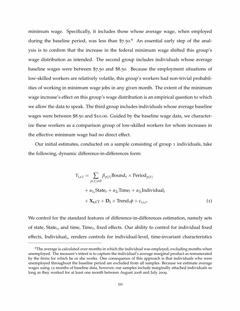
Our initial estimates, conducted on a sample consisting of group 1 individuals, take

the following, dynamic difference-in-differences form:

Yi,s,t = ∑p(t) 6=0

βp(t)Bounds × Periodp(t)

+ α1sStates + α2tTimet + α3iIndividuali

+ Xs,tγ + Di × Trendtφ + εi,s,t. (1)

We control for the standard features of difference-in-differences estimation, namely sets

of state, States, and time, Timet, fixed effects. Our ability to control for individual fixed

effects, Individuali, renders controls for individual-level, time-invariant characteristics

6The average is calculated over months in which the individual was employed, excluding months whenunemployed. The measure’s intent is to capture the individual’s average marginal product as remuneratedby the firms for which he or she works. One consequence of this approach is that individuals who wereunemployed throughout the baseline period are excluded from all samples. Because we estimate averagewages using 12 months of baseline data, however, our samples include marginally attached individuals solong as they worked for at least one month between August 2008 and July 2009.

10

redundant. The vector Xs,t contains time varying controls for each state’s macroeconomic

conditions. In our baseline specification, Xs,t includes the FHFA housing price index,

which proxies for the state-level severity of the housing crisis.7

Equation (1) allows for dynamics motivated by graphical evidence reported in Section

4. Specifically, we show in Section 4 that the prevalence of wages between the old and

new federal minimum declined rapidly beginning in April 2009. We thus characterize

May to July 2009 as a ”Transition” period. Prior months correspond to the baseline, or

period p = 0. We characterize August 2009 through July 2010 as period Post 1 and all

subsequent months as period Post 2. The primary coefficients of interest are βPost 1(t) and

βPost 2(t), which characterize the differential evolution of the dependent variable in states

that were bound by the new federal minimum relative to states that were not bound.

We calculate the standard errors on these coefficients allowing for the errors, εi,s,t, to

be correlated at the state level. Because our treatment group contains 27 states, we do

not face common inference concerns associated with imbalance between the number of

treatment and control states (Bertrand, Duflo, and Mullainathan, 2004).8

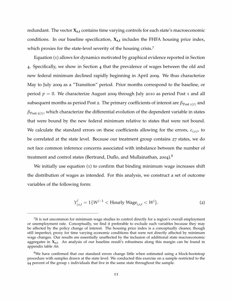
We initially use equation (1) to confirm that binding minimum wage increases shift

the distribution of wages as intended. For this analysis, we construct a set of outcome

variables of the following form:

Y ji,s,t = 1{W j−1 < Hourly Wagei,s,t < W j}. (2)

7It is not uncommon for minimum wage studies to control directly for a region’s overall employmentor unemployment rate. Conceptually, we find it preferable to exclude such variables because they maybe affected by the policy change of interest. The housing price index is a conceptually cleaner, thoughstill imperfect, proxy for time varying economic conditions that were not directly affected by minimumwage changes. Our results are essentially unaffected by the inclusion of additional state macroeconomicaggregates in Xs,t. An analysis of our baseline result’s robustness along this margin can be found inappendix table A6.

8We have confirmed that our standard errors change little when estimated using a block-bootstrapprocedure with samples drawn at the state level. We conducted this exercise on a sample restricted to the94 percent of the group 1 individuals that live in the same state throughout the sample.

11

These Y ji,s,t are indicators that are set equal to 1 if an individual’s hourly wage is between

W j−1 and W j. In practice each band is a 50 cent interval. The βp(t) from these regressions

thus trace out the short and medium run shifts in the wage distribution’s probability

mass function that were associated with binding minimum wage increases.

We then move to our primary outcome of interest, namely the likelihood that an in-

dividual is employed. There are standard threats to interpreting the resulting βp(t) as

unbiased, causal estimates of the effect of binding minimum wage increases. Most im-

portantly, our estimates could be biased by differences in the Great Recession’s severity

in bound states relative to unbound states.

Within the difference-in-differences specification, we directly control for proxies for

the macroeconomic experiences of each state. Recent debate within the minimum wage

literature suggests that such controls may be insufficient.9 Although we find our esti-

mates of equation (1) to be robust to a range of approaches to controlling for heterogene-

ity in macroeconomic conditions, we additionally implement a triple-difference model.

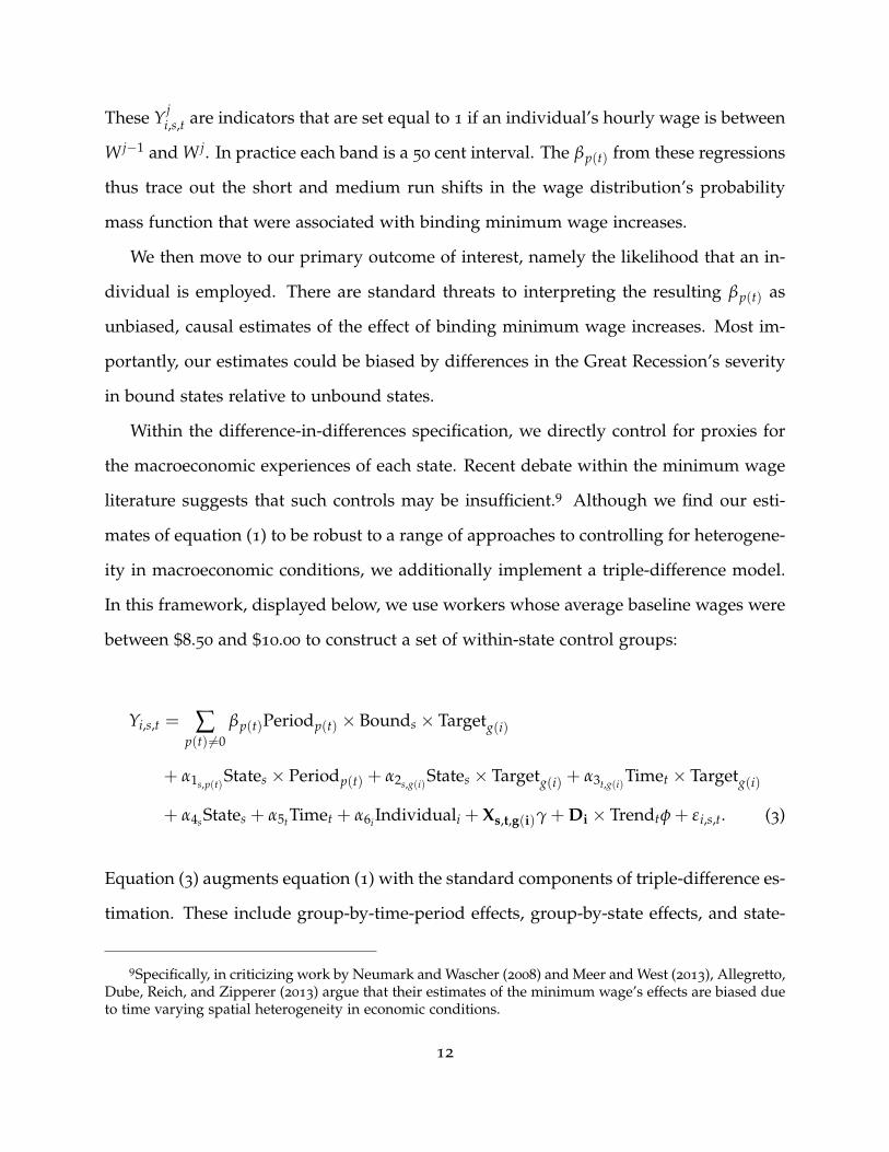
In this framework, displayed below, we use workers whose average baseline wages were

between $8.50 and $10.00 to construct a set of within-state control groups:

Yi,s,t = ∑p(t) 6=0

βp(t)Periodp(t) × Bounds × Targetg(i)

+ α1s,p(t)States × Periodp(t) + α2s,g(i)

States × Targetg(i) + α3t,g(i)Timet × Targetg(i)

+ α4sStates + α5tTimet + α6iIndividuali + Xs,t,g(i)γ + Di × Trendtφ + εi,s,t. (3)

Equation (3) augments equation (1) with the standard components of triple-difference es-

timation. These include group-by-time-period effects, group-by-state effects, and state-

9Specifically, in criticizing work by Neumark and Wascher (2008) and Meer and West (2013), Allegretto,Dube, Reich, and Zipperer (2013) argue that their estimates of the minimum wage’s effects are biased dueto time varying spatial heterogeneity in economic conditions.

12

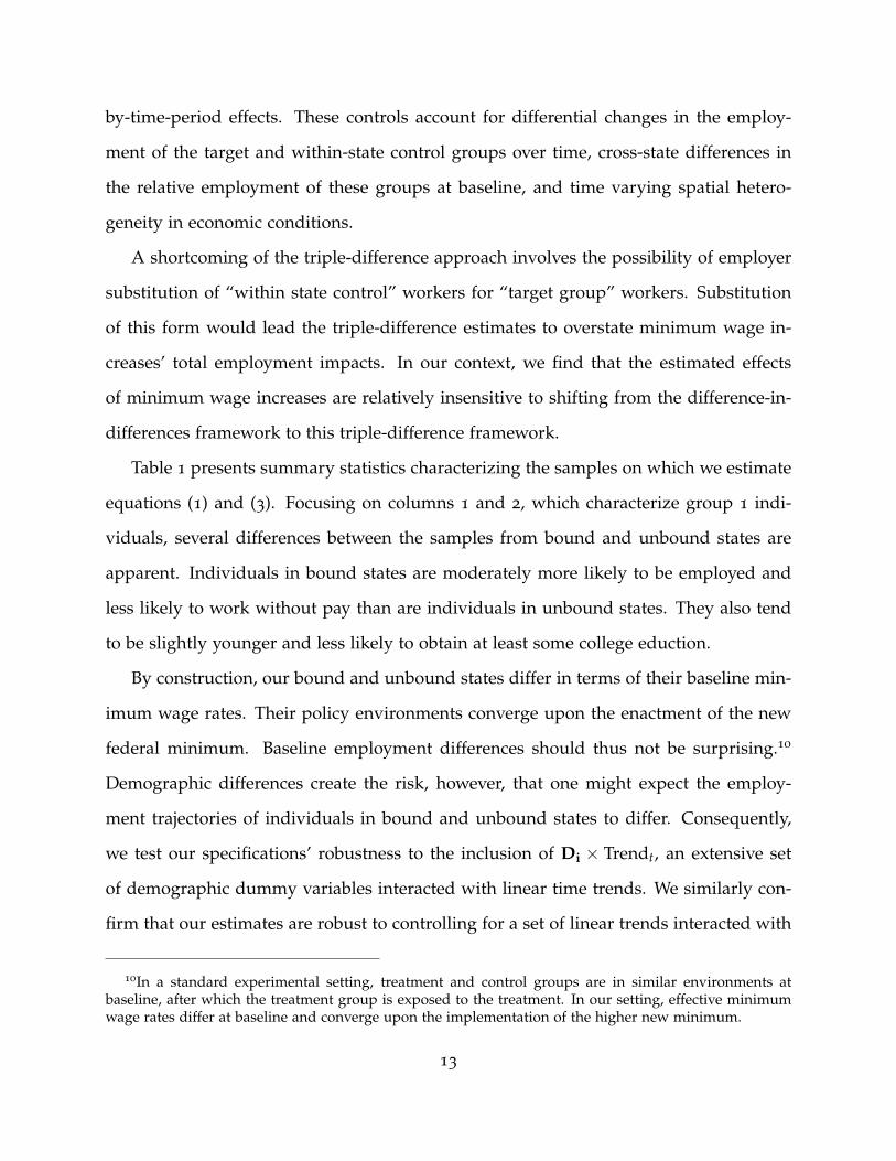
by-time-period effects. These controls account for differential changes in the employ-

ment of the target and within-state control groups over time, cross-state differences in

the relative employment of these groups at baseline, and time varying spatial hetero-

geneity in economic conditions.

A shortcoming of the triple-difference approach involves the possibility of employer

substitution of “within state control” workers for “target group” workers. Substitution

of this form would lead the triple-difference estimates to overstate minimum wage in-

creases’ total employment impacts. In our context, we find that the estimated effects

of minimum wage increases are relatively insensitive to shifting from the difference-in-

differences framework to this triple-difference framework.

Table 1 presents summary statistics characterizing the samples on which we estimate

equations (1) and (3). Focusing on columns 1 and 2, which characterize group 1 indi-

viduals, several differences between the samples from bound and unbound states are

apparent. Individuals in bound states are moderately more likely to be employed and

less likely to work without pay than are individuals in unbound states. They also tend

to be slightly younger and less likely to obtain at least some college eduction.

By construction, our bound and unbound states differ in terms of their baseline min-

imum wage rates. Their policy environments converge upon the enactment of the new

federal minimum. Baseline employment differences should thus not be surprising.10

Demographic differences create the risk, however, that one might expect the employ-

ment trajectories of individuals in bound and unbound states to differ. Consequently,

we test our specifications’ robustness to the inclusion of Di × Trendt, an extensive set

of demographic dummy variables interacted with linear time trends. We similarly con-

firm that our estimates are robust to controlling for a set of linear trends interacted with

10In a standard experimental setting, treatment and control groups are in similar environments atbaseline, after which the treatment group is exposed to the treatment. In our setting, effective minimumwage rates differ at baseline and converge upon the implementation of the higher new minimum.

13

dummy variables associated with each individual’s modal industry of employment over

the baseline period. We further check the robustness of our estimates to a variety of

additional specification modifications. Before presenting our estimates of equations (1)

and (3), we use the following section to graphically present the raw data underlying our

results.

4 Graphical View of the Wages, Employment, and Incomes

of Low-Skilled Workers

Figure 4 presents time series tabulations of the raw data underlying our estimates

of equations (1) and (3). In the panels of column 1, the sample consists of individuals

whose average baseline wages were less than $7.50 per hour. In the panels of column

2, the sample consists of individuals whose average baseline wages were between $7.50

and $10.00 per hour.

The panels in row 1 plot the fraction of individuals that, in any given month, had an

hourly wage between $5.15 and $7.25. Prior to the implementation of the $7.25 federal

minimum, individuals in states that were bound by the federal minimum were much

more likely to have wages in this range than individuals in unbound states. Those in

bound states spent roughly 40 percent of their months in jobs with wages between $5.15

and $7.25, 22 percent of their months unemployed, 17 percent of their months in unpaid

work, and their remaining months in sub-minimum wage jobs (e.g., tipped work) or

in jobs paying more than $7.25. By contrast, individuals in unbound states spent 22

percent of their baseline months in jobs with hourly wages between $5.15 and $7.25.

These fractions began converging in April 2009, three months before the new federal

minimum took effect.11 The observed transition period motivates our accounting for

11The transition window likely reflects a combination of real economic factors and measurement arti-

14

dynamics when estimating equations (1) and (3). By November 2009, individuals in the

bound and unbound states have equal likelihoods of being in jobs with wages between

$5.15 and $7.25.

Panel B shows that the wages of individuals with average baseline wages between

$7.50 and $10.00 per hour were largely unaffected by the increase in the federal mini-

mum. Their probability of having a wage between $5.15 and $7.25 in any given month

was around 5 percent. Prior to the increase in the federal minimum, individuals in

bound states had marginally higher probabilities of having such wages.

The panels in row 2 plot our initial outcome of interest, namely the fraction of in-

dividuals who are employed. Low-skilled workers in states with low minimum wages

initially had moderately higher employment rates, by about 3 percentage points, than

those in states with higher minimums. As wages adjusted to the new federal minimum,

this baseline difference narrows. Over subsequent years, the employment of those in

bound states is, on average, roughly 1 percentage point less than that of low-skilled in-

dividuals in unbound states. Relative to the baseline period, the differential employment

change observable in the raw data is 3 percentage points in the first year and 4 percent-

age points in subsequent years. The data exhibit the seasonality one would expect in the

employment patterns of the relevant populations. The employment series’ convergence

appears linked, at least initially and in part, to a relatively weak summer hiring season

in states bound by the July 2009 increase in the federal minimum.

If these employment changes were driven primarily by cross-state differences in the

severity of the Great Recession, similar (perhaps slightly smaller) changes would be

facts. Employers hiring workers in May and June 2009 may simply have found it sensible to post positionsat the wage which would apply by mid-summer rather than at the contemporaneous minimum. The mea-surement issue involves the SIPP’s 4 month recall windows. Individuals interviewed about their May andJune wages in August 2009 may have mistakenly reported their August wage as their wage throughoutthe recall window. Our response to both potential explanations is to allow for flexible dynamics whenestimating the minimum wage’s effects on employment.

15

expected among workers with modestly greater skills. Panel D shows that such changes

did not occur. Comparing the bound and unbound states, the employment of workers

with average baseline wages between $7.50 and $10.00 moved in parallel over this period.

These data reveal that estimates of equations (1) and (3) will yield similar results.

The panels in row 3 show similar patterns for trends in average monthly income.

During the baseline period, the average incomes of low-skilled individuals in bound

and unbound states evolve similarly. Several months following the increase in the fed-

eral minimum wage, the income growth of low-skilled individuals in the bound states

begins to lag the income growth of low-skilled individuals in unbound states. No such

divergence is apparent among individuals with baseline wages between $7.50 and $10.00.

The data reported in Panel E suggest that the wage gains and employment declines of

targeted workers initially offset one another. Subsequently, declines in employment and

experience accumulation appear to have led the income growth of low-skilled individ-

uals in bound states to lag that of low-skilled workers in unbound states. In Section

5.5 we present a detailed analysis of the factors contributing to these differential income

trajectories.

Figures 5 and 6 present these data in regression-adjusted form. Each marker in the

figures is an estimate of a coefficient of the form βp(t) from equations (1) and (3), where

each p(t) corresponds with an individual month; period p = 0 is April 2009, the month

immediately preceding the transition period. The regression-adjusted changes in em-

ployment and income are largely as one would expect based on the raw data presented

in Figure 4. Adjusting for the housing bubble’s greater severity in unbound states rel-

ative to bound states moderately increases the estimated magnitudes. The following

section presents these and other results in a more summary, tabular fashion.

16

5 Regression Analysis of the Minimum Wage’s Effects

This section presents our estimates of equations (1) and (3). We begin by verifying

that the enacted minimum wage increases shifted the wage distributions of workers with

average baseline wages below $7.50 as intended. We then estimate the minimum wage’s

effect on employment, after which we explore several additional outcomes relevant to

the welfare of affected individuals and their families.

5.1 Effects on Low-Skilled Workers’ Wage Distributions

This section first presents data on the baseline wage distributions of low-skilled work-

ers. It then presents estimates of the extent to which these distributions shift following

binding minimum wage increases. Figure 7 characterizes the wage distributions of work-

ers with average baseline wages below $7.50 (Panel A), average baseline wages between

$7.50 and $8.50 (Panel B), and average baseline wages between $8.50 and $10.00 (Panel

C). The histogram in each panel presents the distribution of each group’s wages during

the baseline period. This distribution, and in particular the frequency of wage rates in

the affected region, is the basis upon which we select our “target” and “within-state

control” groups.12 Note that the histograms exclude the large mass of observations with

no earnings, which includes months spent either unemployed or working without pay.

The histogram for workers with average baseline wages below $7.50 has substantial

mass associated with monthly wage rates between $6.50 and $7.50, as shown in Panel A.

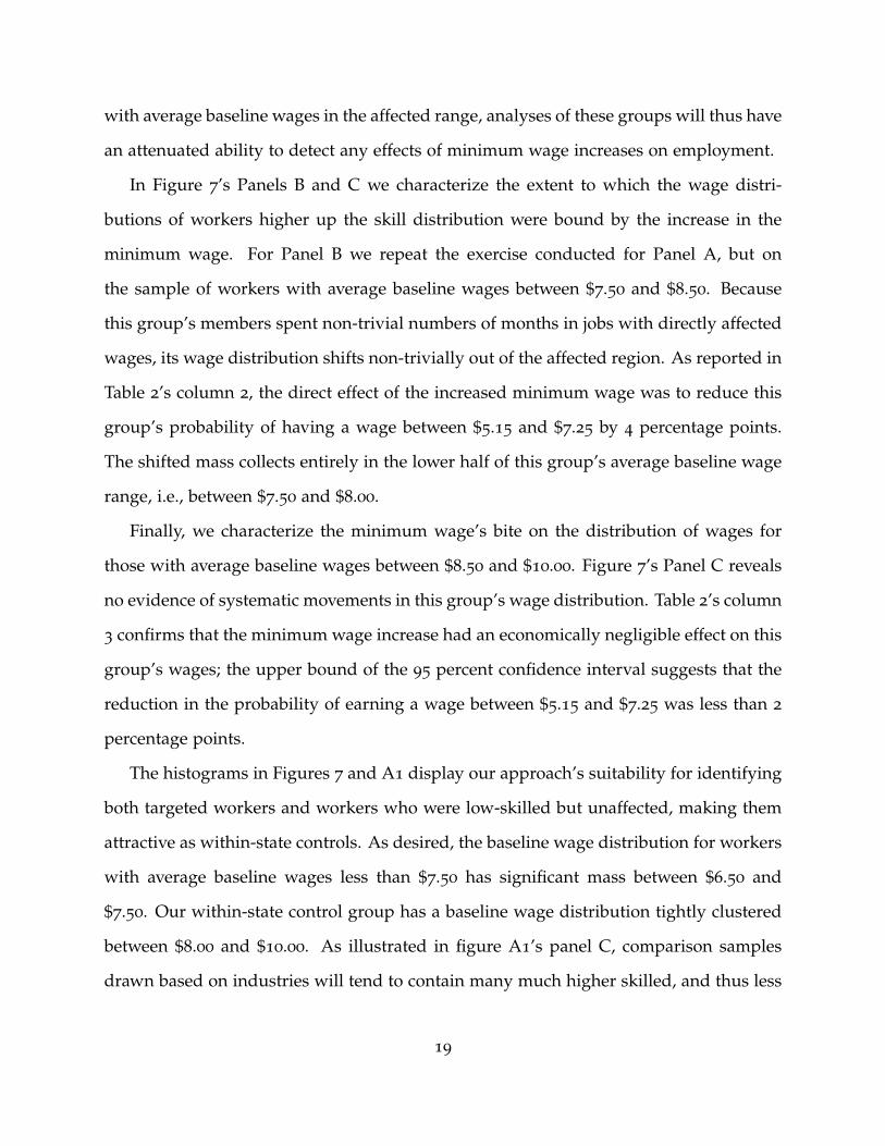
Panel B shows that workers with average baseline wages between $7.50 and $8.50 have

far less mass in the affected region. Nonetheless, this groups’ employment and earnings

12Specifically, we choose our “target” group to be a group with significant baseline mass in the affectedregion and our “within-state control” group to be the lowest-skilled group that spends essentially nobaseline months with wage rates in the affected region. The estimated effects of binding minimum wageincreases on these distributions confirms that the former’s distribution shifted significantly while thelatter’s did not.

17

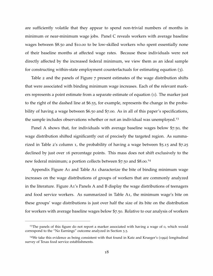
are sufficiently volatile that they appear to spend non-trivial numbers of months in

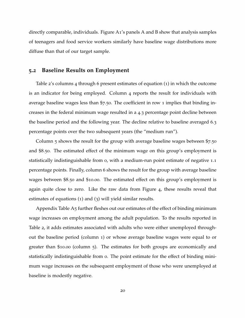
minimum or near-minimum wage jobs. Panel C reveals workers with average baseline

wages between $8.50 and $10.00 to be low-skilled workers who spent essentially none

of their baseline months at affected wage rates. Because these individuals were not

directly affected by the increased federal minimum, we view them as an ideal sample

for constructing within-state employment counterfactuals for estimating equation (3).

Table 2 and the panels of Figure 7 present estimates of the wage distribution shifts

that were associated with binding minimum wage increases. Each of the relevant mark-

ers represents a point estimate from a separate estimate of equation (1). The marker just

to the right of the dashed line at $6.55, for example, represents the change in the proba-

bility of having a wage between $6.50 and $7.00. As in all of this paper’s specifications,

the sample includes observations whether or not an individual was unemployed.13

Panel A shows that, for individuals with average baseline wages below $7.50, the

wage distribution shifted significantly out of precisely the targeted region. As summa-

rized in Table 2’s column 1, the probability of having a wage between $5.15 and $7.25

declined by just over 16 percentage points. This mass does not shift exclusively to the

new federal minimum; a portion collects between $7.50 and $8.00.14

Appendix Figure A1 and Table A1 characterize the bite of binding minimum wage

increases on the wage distributions of groups of workers that are commonly analyzed

in the literature. Figure A1’s Panels A and B display the wage distributions of teenagers

and food service workers. As summarized in Table A1, the minimum wage’s bite on

these groups’ wage distributions is just over half the size of its bite on the distribution

for workers with average baseline wages below $7.50. Relative to our analysis of workers

13The panels of this figure do not report a marker associated with having a wage of 0, which wouldcorrespond to the “No Earnings” outcome analyzed in Section 5.5.

14We take this evidence as being consistent with that found in Katz and Krueger’s (1992) longitudinalsurvey of Texas food service establishments.

18

with average baseline wages in the affected range, analyses of these groups will thus have

an attenuated ability to detect any effects of minimum wage increases on employment.

In Figure 7’s Panels B and C we characterize the extent to which the wage distri-

butions of workers higher up the skill distribution were bound by the increase in the

minimum wage. For Panel B we repeat the exercise conducted for Panel A, but on

the sample of workers with average baseline wages between $7.50 and $8.50. Because

this group’s members spent non-trivial numbers of months in jobs with directly affected

wages, its wage distribution shifts non-trivially out of the affected region. As reported in

Table 2’s column 2, the direct effect of the increased minimum wage was to reduce this

group’s probability of having a wage between $5.15 and $7.25 by 4 percentage points.

The shifted mass collects entirely in the lower half of this group’s average baseline wage

range, i.e., between $7.50 and $8.00.

Finally, we characterize the minimum wage’s bite on the distribution of wages for

those with average baseline wages between $8.50 and $10.00. Figure 7’s Panel C reveals

no evidence of systematic movements in this group’s wage distribution. Table 2’s column

3 confirms that the minimum wage increase had an economically negligible effect on this

group’s wages; the upper bound of the 95 percent confidence interval suggests that the

reduction in the probability of earning a wage between $5.15 and $7.25 was less than 2

percentage points.

The histograms in Figures 7 and A1 display our approach’s suitability for identifying

both targeted workers and workers who were low-skilled but unaffected, making them

attractive as within-state controls. As desired, the baseline wage distribution for workers

with average baseline wages less than $7.50 has significant mass between $6.50 and

$7.50. Our within-state control group has a baseline wage distribution tightly clustered

between $8.00 and $10.00. As illustrated in figure A1’s panel C, comparison samples

drawn based on industries will tend to contain many much higher skilled, and thus less

19

directly comparable, individuals. Figure A1’s panels A and B show that analysis samples

of teenagers and food service workers similarly have baseline wage distributions more

diffuse than that of our target sample.

5.2 Baseline Results on Employment

Table 2’s columns 4 through 6 present estimates of equation (1) in which the outcome

is an indicator for being employed. Column 4 reports the result for individuals with

average baseline wages less than $7.50. The coefficient in row 1 implies that binding in-

creases in the federal minimum wage resulted in a 4.3 percentage point decline between

the baseline period and the following year. The decline relative to baseline averaged 6.3

percentage points over the two subsequent years (the “medium run”).

Column 5 shows the result for the group with average baseline wages between $7.50

and $8.50. The estimated effect of the minimum wage on this group’s employment is

statistically indistinguishable from 0, with a medium-run point estimate of negative 1.1

percentage points. Finally, column 6 shows the result for the group with average baseline

wages between $8.50 and $10.00. The estimated effect on this group’s employment is

again quite close to zero. Like the raw data from Figure 4, these results reveal that

estimates of equations (1) and (3) will yield similar results.

Appendix Table A5 further fleshes out our estimates of the effect of binding minimum

wage increases on employment among the adult population. To the results reported in

Table 2, it adds estimates associated with adults who were either unemployed through-

out the baseline period (column 1) or whose average baseline wages were equal to or

greater than $10.00 (column 5). The estimates for both groups are economically and

statistically indistinguishable from 0. The point estimate for the effect of binding mini-

mum wage increases on the subsequent employment of those who were unemployed at

baseline is modestly negative.

20

5.3 Contrasting Approaches To Evaluating the Minimum Wage

In further analysis, we estimate the minimum wage’s effects on the employment

of populations studied frequently in the literature, namely teenagers and food service

workers. More specifically, we estimate equation (1) on a sample selected to include

individuals who were teenagers or for whom food service was the modal industry of

employment during the baseline period. Column 5 of Appendix Table A1 reports our

estimate that binding minimum wage increases reduced this sample’s medium-run em-

ployment by 3.9 percentage points. Column 6 reports an estimate near 0 for the mini-

mum wage increase’s effect on the employment of manufacturing workers, whose wage

distribution was unaffected. Our specification thus passes the primary falsification test

emphasized in a recent exchange involving Dube, Lester, and Reich (2010), Meer and

West (2013), and Dube (2013).

We draw two lessons from comparing the estimates associated with our baseline sam-

ple and the sample of teenagers and food service workers. First, the estimates associated

with teenagers and food service workers reinforce the conclusion that this period’s min-

imum wage increases reduced the employment of low-skilled workers. Second, they

point to a potential line of reconciliation between some of the literature’s null results

and our finding of significant disemployment effects.

As emphasized by Sabia, Burkhauser, and Hansen (2012), cross-study comparisons

require scaling estimates by the extent to which alternative analysis samples are actually

affected by the minimum wage. Comparisons involving estimates from industry-level

studies are particularly difficult because such studies typically lack the individual-level

data required to directly estimate the minimum wage’s bite on the underlying workers’

wage distribution.15 We estimate that the wage distribution of our target sample was

15The extent of the minimum wage’s bite on populations under study is often inferred from CPSdata. A variety of measurement issues make it rare, however, to have directly comparable estimatesof the minimum wage’s effects on the wage distributions of alternative study populations. Relevant

21

nearly twice as affected as the wage distribution of teenagers and food service workers.

Our estimates of the minimum wage increase’s effects on these groups’ employment

were similarly proportioned. It is thus important to note that, all else equal, estimates

of a minimum wage increase’s effects on relatively untargeted groups will be attenuated

and, as a result, more prone to type II error.

Appendix Table A4 provides a further line of comparison between our results and

the findings of industry-specific analyses of the minimum wage. In our baseline analy-

sis and our analysis of teenagers and food service workers, we estimate the minimum

wage’s effects on the employment of low-skilled individuals. By contrast, analyses of

industry-level data estimate the minimum wage’s effects on total employment in low-

skill-intensive industries. In Table A4 we present estimates of the minimum wage’s effect

on the probability that any given individual is employed in the food service sector. For

the full sample of individuals aged 16 to 64, the estimated effect on food service employ-

ment is economically negligible and statistically indistinguishable from 0. As revealed

in column 2, this masks a 3 percentage point decline in food service employment among

individuals with average baseline wages below $7.50. Column 3 reports an offsetting

increase in the food service employment of workers with higher baseline wage rates.16

We draw two additional lessons from this analysis. First, we note that the minimum

wage’s effects may vary significantly across industries, making it difficult to extrapolate

from industry-specific estimates to aggregate employment. In a standard model, the

measurement issues include survey reporting error and variation in the minimum wage’s applicabilitydue to exceptions such as those made for tipped workers. Sabia, Burkhauser, and Hansen (2012) and thepresent study’s appendix materials are the only recent examples of such analyses of which we are aware.An alternative approach to inferring the minimum wage increase’s direct effect involves using industry- orfirm-level data to estimate its effect on average earnings per worker, as in Dube, Lester, and Reich (2010).In such data, however, increases in earnings per worker may reflect either increases in the earnings of thelow-skilled or substitution of high-skilled workers for low-skilled workers. Absent additional information,such data will not enable researchers to distinguish between these outcomes.

16Because the sample in column 3 is roughly 10 times the size of the sample in column 1, the -0.03

employment effect from column 2 is essentially fully offset by the estimate of 0.003 from column 3.

22

determinants of an industry’s adaptation to a minimum wage change include its ability

to substitute between low-skilled workers, high-skilled workers, and capital, as well as

the elasticity of demand for its output. The results in Table A4 provide evidence that,

during the period we study, food-service employers had significant scope for substituting

between low- and high-skilled workers.

Second, the results highlight that substitution between low- and high-skilled workers

can complicate efforts to evaluate the minimum wage’s effects using data on industry-

level wage bills and employment. In such data, the results in Table A4 would be indis-

tinguishable from an outcome in which an increase in the minimum wage non-trivially

increased per-worker earnings and had minimal effects on employment. In the setting

we analyze, this mistaken interpretation would leave the impression that the minimum

wage had achieved its objective of increasing low-skilled workers’ incomes at little cost.

5.4 Robustness of the Estimated Employment Effects

Table 2’s primary result of interest is column 4’s estimate of the minimum wage

increase’s effect on the employment of targeted workers. Tables 3 and A6 present an

analysis of this result’s robustness. In Table 3, estimates in Panel A are of equation

(1)’s difference-in-differences model. Estimates in Panel B are of equation (3)’s triple

difference model, in which we use workers with average baseline wages between $8.50

and $10.00 as a within state control group.

The result in column 1 of Panel A replicates the finding from Table 2’s column 4. The

result in column 1 of Panel B shows this result to be robust to estimating the minimum

wage’s effect using the triple-difference framework. The medium run estimate implies

that binding minimum wage increases reduced the target group’s employment rate by

5.9 percentage points.

Column 2 presents results in which we exclude our controls for states’ macroeco-

23

nomic conditions. Not controlling for variation in the housing bubble’s severity across

states reduces the estimated coefficients by 2 percentage points. The estimated em-

ployment decline is 4.2 percentage points in the difference-in-differences model and 3.8

percentage points in the triple-difference model. This reflects the fact that, as shown in

Figure 3, the housing bubble was more severe in unbound states than in bound states.

We further explore the relevance of macroeconomic controls in Table A5, which we dis-

cussion momentarily.

Column 3 shows that our results are robust to controlling for state-specific linear

time trends.17 In the difference-in-differences specification, including these controls in-

creases the estimated medium-run coefficient from 6.3 to 7.2 percentage points. Column

4 shows that our results are relatively insensitive to controlling for exhaustive sets of

age, education, and family-size indicators interacted with linear time trends.18 Differen-

tial trajectories linked to moderate differences in the demographic characteristics of the

group 1 samples in bound and unbound states thus appear unlikely to underlie our es-

timates. We find the same to be true of differences associated with bound and unbound

states’ industrial compositions.

The remaining columns involve changes in our sample inclusion criteria. Column

5 shows that our results are robust to requiring that, for inclusion in the final sample,

17We share Meer and West’s (2013) concern that, because of the dynamics with which minimum-wage induced employment losses may unfold, direct inclusion of state-specific trends is not a particularlyattractive method for controlling for the possibility of differential changes in the economic conditions ofeach state over time. The dynamics allowed for by our Transition, Post 1, and Post 2 periods turn out,in this context, to be sufficient to render state-specific trends largely irrelevant. This is less true in lateranalysis of the minimum wage’s effects on income. The minimum wage may affect income through directdisemployment effects, subsequent effects on experience accumulation, and related effects on trainingopportunities. The latter effects will be realized as effects on income growth, making Meer and West’s(2013) critique particularly pertinent.

18We similarly find our results to be robust to controlling for time trends interacted with dummyvariables for 20 cent bins in our measure of average baseline wages (result not shown). This check isaddressed at the concern that, because minimum wage workers in unbound states had relatively highwages at baseline, their employment and earnings trajectories might differ for reasons related to meanreversion.

24

individuals appear in the sample for at least 42 months rather than our baseline re-

quirement of 36 months. The specifications in columns 6 and 7 involve modifications to

our criteria for categorizing the bound and unbound states. Column 6 drops unbound

states in which the January 2008 minimum wage was less than $7.00, as such states were

moderately bound by subsequent increases in the federal minimum. Removing these 4

states (Arizona, Florida, Missouri, and West Virginia) from the control group modestly

increases the medium-run point estimate to 6.7 percentage points in the difference-in-

differences model and leaves the triple-difference estimate unchanged at 5.9 percentage

points. Finally, column 7 removes from the sample any bound state with a January 2009

minimum wage above $6.55. Our baseline designation uses states’ January 2008 mini-

mum wage rates to ensure that it is based on decisions made before our sample begins.

We observe that 4 states (Montana, Nevada, New Hampshire, and New Mexico) with

January 2008 minimum wage rates below $6.55 voluntarily increased their minimums

before they were required to do so. Dropping these states from the sample modestly

decreases the medium-run estimates in both the difference-in-differences and triple dif-

ference specifications (by several tenths of a percentage point in each case).

Appendix Table A6 provides additional evidence regarding the relevance of controls

for differences in the severity of the Great Recession in bound and unbound states.

Columns 1 and 2 replicate columns 1 and 2 from panel A of Table 3. As an alterna-

tive to controlling for the housing price index, column 3 adds controls for state level

income and employment per capita. Column 4 adds controls for stimulus spending per

capita and two additional variables. The first, “Predicted State Income,” is a projec-

tion of state-specific changes in aggregate output that are predictable on the basis of

each state’s historical relationship with the national business cycle. The second, “Pre-

dicted State Employment,” is a projected change in employment based on each states’

baseline industrial composition and subsequent industry-specific employment growth

25

at the national level (Bartik, 1991; Blanchard and Katz, 1992). The inclusion of these

alternative macroeconomic control variables increases the estimated effect of binding

minimum wage increases relative to specifications that include no such controls. When

these variables are included alongside the housing price index, the estimates are essen-

tially unchanged from the baseline. The housing price index consistently emerges as

a stronger predictor of employment among low-skilled individuals than the alternative

macroeconomic control variables. The specifications in columns 6 and 7 incorporate

state-specific trends, the full sets of trends in various demographic characteristics, and

trends specific to each individual’s modal industry of employment at baseline. In both

of these specifications, we estimate that binding minimum wage increases resulted in 7

percentage point declines in the employment of low-skilled workers.

5.5 Further Employment Outcomes, Average Income, and Poverty

Tables 4 and 5 report the results of a more in depth analysis of the minimum wage’s

effects on employment and income related outcomes. In Table 4’s second column we

present evidence of a novel channel through which job markets may respond to min-

imum wage increases. Specifically, we show that binding minimum wage increases

resulted in an increase in the probability that targeted individuals work without pay,

perhaps in internships, by 2 percentage points. Between disemployment and work with-

out pay, column 3 reports a combined 8 percentage point reduction in paid employment.

Appendix Tables A7 and A8 show that our estimates of both the “internship” effect and

the total effect on paid employment are robust to the same set of specification changes

as our estimate of the traditional disemployment effect. Estimates of the medium-run

effect on the probability of working without pay range from 1.3 to 2.5 percentage points.

Estimates of the total effect on the probability of paid employment range from 6.0 to 9.4

percentage points.

26

Table 5 presents estimates of these effects separately for individuals with and without

at least some college education. Here it is important to keep in mind that all of the

individuals in the sample have average baseline wages less than $7.50. Those with at

least some college education are relatively likely to be current students or very early in

their careers.

We find that low-skilled workers with at least some college education underlie the

entirety of the minimum wage’s effect on the likelihood of working without pay. The in-

crease in the federal minimum wage made low-skilled workers with at least some college

education 4 percentage points (roughly 20 percent) more likely to work without pay. For

individuals with less education, the entirety of the minimum wage’s effect on paid em-

ployment comes through unemployment. These findings are suggestive of a difference

in the entry-level positions of high- and low-education workers. Entry positions sought

by high-education workers appear relatively interchangeable with unpaid internships.

Appendix Tables A11 and A12 report further analysis of demographic heterogeneity in

our estimates of the minimum wage’s effects.

Returning to outcomes more central to the minimum wage’s redistributive proper-

ties, Table 4’s columns 4 and 5 report the effect of binding minimum wage increases on

average monthly incomes. Column 4 reports the effect on individual-level income while

column 5 reports the effect on family-level income. We censor these outcomes at $7,500

and $22,500 per month respectively; this affects fewer than 1 percent of observations,

which are associated with incomes far beyond those attainable through minimum wage

employment. In our difference-in-differences specification, we estimate that binding

minimum wage increases reduced the average monthly income of low-skilled workers

by $97 in the short-run and $153 in the medium-run. Results are slightly larger, though

estimated with significantly less precision, in our triple-difference specification. Robust-

ness across these specifications is particularly relevant for outcomes involving income.

27

Specifically, it reassures us that the results are not spuriously driven by growth in the

control-group workers’ incomes towards the relatively high per capita incomes associ-

ated with unbound states (recall Panel D of Figure 3).

Figure 6 more fully highlights the dynamics underlying these results. In the figure it

is apparent that employment losses and wage gains offset one another over the transition

months. Accumulating employment losses and lost wage gains associated with lost ex-

perience begin outstripping the legislated wage gains in subsequent periods. Appendix

Table A9 reports the robustness of the estimated effects on average income to the same

set of specification checks as the outcomes previously analyzed.

To better understand these estimates, note that targeted individuals in bound states

had positive earnings in 61 percent of baseline months. In 22 percent they were unem-

ployed and in 17 percent they worked with 0 earnings. Average income for the target

sample was $770 across all baseline months, and thus roughly $1,260 in months with

positive earnings. For the short run (i.e., year 1), we estimated a 6 percentage point de-

cline in the probability of having positive earnings. This effect is thus directly associated

with an average decline of roughly $75, or $1, 260× 0.06. The decline in months with

positive earnings rises to 8 percentage points over the following two years, implying

a direct earnings decline of $100. Gains for workers successfully shifted from the old

minimum to the new minimum offset very little of this decline.19

19Recall that we estimated a 16 percentage point decline in the probability of having a wage between$5.15 and $7.25. Nearly half of this turns out to involve shifts into unemployment or unpaid work. Thewage increase for the remaining 8 percentage points was roughly 10 percent (from the $6.55 minimumfor 2008 to the $7.25 minimum for 2009). A 10 percent increase on the $1,260 base, realized by 8 percentof workers, averages to a gain of $10. Measurement error in self-reported wage rates likely leads thisapproach to understate the true gain; it likely attenuates our estimates of the minimum wage’s bite on thewage distributions of low-skilled workers. An alternative approach, likely generating an upper bound, isto infer the minimum wage’s bite from the data displayed in Figure 4. Figure 4’s panel A showed that low-skilled workers in bound states saw their probability of reporting a wage between $5.15 and $7.25 declineby roughly 35 percentage points from a base of just over 40 percentage points. Even the 35 percentagepoints of bite one could maximally infer from figure 4 implies quite modest offsets of the income lossesassociated with disemployment, work without pay, and lost experience accumulation.

28

The effects of lost employment rise over time due to lost experience. Minimum wage

workers tend to be on the steep portion of the wage-experience profile (Murphy and

Welch, 1990). Using mid-1980s SIPP data, Smith and Vavrichek (1992) found that 40 per-

cent of minimum wage workers experienced wage gains within 4 months and that nearly

two-thirds did so within 12 months. The median gain among the one-year gainers was

a substantial 20 percent. Among those unemployed or working without pay, foregone

wage growth of these magnitudes brings the implied medium-run earnings decline to

$130.20 Targeted workers who maintain employment may also experience slow earnings

growth if employers reduce opportunities for on the job training.

Our estimates of the minimum wage increase’s effect on income are initially some-

what surprising. As illustrated above, however, they follow from the magnitude of our

estimated employment effects coupled with three more conceptually novel factors. These

factors include our finding of an “internship” effect, effects on income growth through

reduced experience accumulation, and the fact that direct effects on wages were smaller

than typically assumed.

We emphasize that our analysis involves increases in the minimum wage that took

effect during a period of significant labor shedding. The employment, internship, and

experience-accumulation effects are thus likely to have been particularly potent during

this historical episode. Finally we note that our income point estimates come with con-

siderable uncertainty. The associated standard errors are sufficiently large that we cannot

rule out relatively modest declines in average income.

Returning to Table 4, we estimate the minimum wage’s effects on family-level out-

comes. On average in our sample, each targeted worker is in a family with 1.3 targeted

workers. This is roughly the average of the ratio of our estimates of the minimum wage

20Two years of early-career earnings growth at 15 percent per year would bring earnings from a baselineof $1,260 to $1,670. An 8 percentage point decline in months at such earnings implies an average reductionof $133.

29

increase’s effect on family-level income to its effect on individual-level income. In the

triple-difference specifications, for example, the short-run effect on individual-level in-

come is $112 per month while the estimated effect on family-level income is $120 (the

medium-run estimates are $185 and $300).

Finally, column 6 shows that the effect of binding minimum wage increases on the

incidence of poverty was statistically indistinguishable from 0. Unsurprisingly, given

our finding on family-level earnings, the point estimate for the medium-run effect on

the likelihood of being in poverty is positive. The absence of a decline in poverty echoes

findings by Burkhauser and Sabia (2007), Sabia and Burkhauser (2010), Neumark and

Wascher (2002), and Neumark, Schweitzer, and Wascher (2005), as well as a summary of

earlier evidence by Brown (1999).

5.6 Transitions from Low-Wage Work into Middle Class Earnings

We next analyze income growth through the lens of economic mobility, a topic of

significant recent interest (Kopczuk, Saez, and Song, 2010; Chetty, Hendren, Kline, and

Saez, 2014; Chetty, Hendren, Kline, Saez, and Turner, 2014). Concern regarding the

minimum wage’s effects on upward mobility has a long history (Feldstein, 1973). A

potential mechanism for such effects, namely the availability of on-the-job training, has

received some attention in the literature (Hashimoto, 1982; Arulampalam, Booth, and

Bryan, 2004). We are not aware, however, of direct evidence of the minimum wage’s

effects on individuals’ transitions into employment at higher wages and earnings levels.

Because we observe individuals for four years, we are able to track transitions of low-

wage workers into middle and lower middle class earnings. The data reveal that initially

low-wage workers spend non-trivial numbers of months with earnings exceeding those

of a full time, minimum wage worker. Consider earnings above $1500, which could

be generated by full time work at $8.80 per hour. During the first year of our sample,

30

workers with average baseline wages less than $7.50 earn more than $1500 in 8 percent

of months. By the sample’s last two years this rises, adjusting for inflation, to 18 percent.

We investigate the minimum wage’s effects on the likelihood of reaching such earnings.

Table 6 reports the results. We find significant declines in economic mobility, in

particular for transitions into lower middle class earnings. For the full sample with

average baseline wages less than $7.50, the difference-in-differences estimate implies that

binding minimum wage increases reduced the probability of reaching earnings above

$1500 by 4.9 percentage points. This represents a 24 percent reduction relative to the

control group’s medium-run probability of attaining such earnings. As with previous

results, this finding cannot readily be explained by cross-state differences in economic

conditions. Netting out the experience of individuals with baseline wages between $8.50

and $10.00 moderately increases the point estimate to 5.4 percentage points (26 percent).

The estimated reductions in the probability of reaching lower middle class earnings

levels are particularly meaningful for low-skilled workers with no college education. In

the difference-in-differences specification, the estimated decline in this group’s proba-

bility of earning more than $1500 per month is 4.9 percentage points (see column 2).

In the triple-difference specification the estimate is 8.2 percentage points. Declines of

these magnitudes represent 32 and 54 percent declines relative to the control group’s

probability of reaching such earnings. For those with at least some college education,

the estimated declines average a more moderate 4 percentage points, equivalent to 17

percent of the control group’s probability of reaching such earnings. Figure 8 presents

the raw data underlying these results, and Appendix Table A10 reports the robustness of

the estimated effects to the same set of specifications checks as the outcomes previously

analyzed.

We next examine the probability of reaching the middle-income threshold of $3000

per month. For the full sample, we estimate that binding minimum wage increases

31

reduced this probability by 1.8 percentage points. In the difference-in-differences spec-

ification, this estimate is statistically distinguishable from 0 at the 10 percent level; in

the triple-difference specification this is not the case, although the point estimate is es-

sentially unchanged. Though our sub-sample analysis has little precision, the average

medium-run effect appears to be driven primarily by those with at least some college

education. The full sample decline of 1.7 percentage points is a non-trivial 26 percent of

the control group’s medium-run probability of reaching such earnings.

We interpret the evidence as implying that binding minimum wage increases re-

duced the medium-run class mobility of low-skilled workers. Such workers became

significantly less likely to rise to the lower middle class earnings threshold of $1500 per

month. The reduction was particularly large for low-skilled workers with relatively little

education.

The dynamics of our estimated employment and class mobility results are suggestive

of the underlying mechanisms. Our employment results emerge largely during the first

year following the increase in the federal minimum wage. By construction, our mobil-

ity outcomes are not outcomes that can be affected by the loss of a full time minimum

wage job. Effects on mobility into lower middle class earnings only emerge over subse-

quent years. It appears that binding minimum wage increases blunted these workers’

prospects for medium-run economic mobility by reducing their short-run access to op-

portunities for accumulating experience and developing skills. This period’s minimum

wage increases may thus have made the first rung on the earnings ladder more difficult

for low-skilled workers to reach.

5.7 Contrasting the Minimum Wage and the Earned Income Tax Credit

The minimum wage is one of many policies implemented with an objective of in-

creasing the effective wage rates or earnings of low-skilled workers. In the U.S. context,

32

the policy most obviously interchangeable with the minimum wage is the Earned Income

Tax Credit (EITC).21 Analyses of the relative effectiveness of redistributing via wage reg-

ulation versus the tax code date at least as far back as Stigler (1946), whose discussion

ranged from potential employment effects to target-efficiency and administrative com-

plexity. Our estimates speak to the minimum wage’s effectiveness in achieving its direct

objective of increasing the incomes of targeted workers. In the paragraph below, we

contrast our estimates with the relevant results from the literature on the EITC.

Our estimates provide evidence that binding minimum wage increases reduced the

employment, average income, and income growth of low-skilled workers over short-

and medium-run time horizons. By contrast, analyses of the EITC have found it to in-

crease both the employment of low-skilled adults and the incomes available to their fam-

ilies (Eissa and Liebman, 1996; Meyer and Rosenbaum, 2001; Eissa and Hoynes, 2006).

The EITC has also been found to significantly reduce both inequality (Liebman, 1998)

and tax-inclusive poverty metrics, in particular for children (Hoynes, Page, and Stevens,

2006). Evidence on outcomes with long-run implications further suggest that the EITC

has tended to have its intended effects. Dahl and Lochner (2012), for example, find

that influxes of EITC dollars improve the academic performance of recipient house-

holds’ children. This too contrasts with our evidence on the minimum wage’s effects on

medium-run economic mobility.

21The potential substitutability and complementarity of regulatory and tax-financed redistributive mea-sures is an underlying theme in Clemens’s (2014) analysis of community rating regulations in insurancemarkets.

33

6 Implications for Changes in Aggregate Employment Over

the Great Recession

Between December 2006 and December 2012, the average effective minimum wage

rose from $5.88 to $7.56 across the United States. Over this same time period, the

employment-to-population ratio for adults aged 16 to 64 declined by nearly 5 percent-

age points. Clemens and Wither (2014) more fully characterize this period’s employ-

ment declines, including its demographic and cross-country dimensions. Sustained U.S.

employment declines were particularly dramatic for young adults aged 15 to 24. As

of September 2014, this group’s employment remained down by 7.5 percentage points

from its pre-recession peak. Additionally, U.S. employment declines generally exceeded

those that occurred in other advanced economies.22 These dimensions of the data sug-

gest that U.S.-specific developments in low-skilled labor markets underlie much of the

slump in U.S. employment. We thus conclude by considering our results’ implications

for the relationship between minimum wage increases and these sustained employment

declines.

Panel B of Appendix Table A5 presents the full set of results required to infer aggre-

gate employments effects from our estimates. The table presents estimates of equation

(1) on sub-samples that fully partition the set of adults aged 16 to 64. Column 2 repli-

cates our baseline estimate that binding minimum wage increases reduced the target

population’s employment rate by 6 percentage points. The remaining estimates provide

evidence that these minimum wage increases had little if any effect on the employment

of other groups, which is the assumption maintained for this section’s calculation.23

22See Hoffmann and Lemieux (2014) for related characterizations of cross-country developments inunemployment rates.

23Note that for this exercise the estimated effects on other groups’ employment must be directly inter-preted as estimates of the minimum wage increase’s effects rather than as evidence supporting the validity

34

Several factors make extrapolating our results into changes in national employment-

to-population ratios somewhat speculative. First, as emphasized earlier, we have likely

estimated both the full effect of the July 2009 increase and some dynamic effects of the

July 2008 increase in the federal minimum. In July 2009, the differential increase between

bound and unbound states was $0.58. We may more plausibly be detecting the effect of

an increase equivalent to $0.80 or $0.90 (roughly 13 percent of initial levels). Second, the

employment effects of minimum wage increases may be non-linear, with larger effects

for final increments than for initial increases. Third, the nominal value of the minimum

wage has more purchasing power, and hence more bite, in the typical bound state than in

the typical unbound state. Figure 3 showed bound states to have relatively low incomes

and housing costs, making it unsurprising that they had not voluntarily brought their

minimums to the levels seen in the unbound states. These issues inform the lower and

upper bounds we place on our estimates of the minimum wage’s aggregate effects.

The calculation proceeds as follows. Our baseline estimate is that binding minimum

wage increases reduced the employment of workers with average baseline wages below

$7.50 by 6 percentage points (8 percent).24 For this section’s purposes, the estimates

reported in Appendix Table A5 make us reasonably confident in treating the decline in

the target group’s employment as the sole effect of this period’s binding minimum wage

increases on aggregate employment. Applying the relevant weights, the target sample

represents 7.4 percent of the U.S. population aged 16 to 64. A 6 percentage point decline

of our estimates of the minimum wage’s effect on the target group.

24The implied elasticity of the sample-group’s employment with respect to the minimum wage is thusaround two-thirds (8 percent divided by the 13 percent from the previous paragraph). Comparing elastic-ities across studies is more difficult than one might expect due to the need to scale appropriately by theextent to which each study’s “target” group was actually affected by the relevant minimum wage increase(Sabia, Burkhauser, and Hansen, 2012). This is made difficult by the fact that most minimum wage studiesdo not directly estimate the extent to which legislated minimum wage changes shift the wage distributionsof the populations whose employment they study. As shown in Appendix Figure 1, standard approachesidentify targeted individuals with significantly less precision than the approach employed in the currentstudy. While our full-group elasticity is thus larger than those estimated in most past research, it appearsmore moderately sized when compared on an appropriately scaled basis.

35

in this group’s employment thus implies a 7.4× 0.06 = 0.45 percentage point decline

in the employment-to-population ratio. We take this to be a conservative lower bound

estimate for the total effect of the $1.68 average rise in the effective minimum wage across

the country. We consider twice this amount, or 0.90 percentage points, to be a reasonable

upper bound. Our best estimate is that this period’s minimum wage increases resulted in

a 0.7 percentage point decline in the national employment-to-population ratio for adults

aged 16 to 64. This accounts for 14 percent of the total decline in the employment-to-

population ratio over this time period.

7 Conclusion

We investigate the effects of recent federal minimum wage increases on the employ-

ment and income trajectories of low-skilled workers. While the wage distribution of

low-skilled workers shifts as intended, the estimated effects on employment, income, and

income growth are negative. We infer from our employment estimates that minimum

wage increases reduced the national employment-to-population ratio by 0.7 percentage

point between December 2006 and December 2012. As noted above, this accounts for 14

percent of the national decline in the employment-to-population ratio over this period.

We also present evidence of the minimum wage’s effects on low-skilled workers’ eco-

nomic mobility. We find that binding minimum wage increases significantly reduced

the likelihood that low-skilled workers rose to what we characterize as lower middle

class earnings. This curtailment of transitions into lower middle class earnings began

to emerge roughly one year following initial declines in low wage employment. Reduc-

tions in upward mobility thus appear to follow reductions in access to opportunities for

accumulating work experience.

36

References

Addison, J. T., M. L. Blackburn, and C. D. Cotti (2013): “Minimum wage increases in

a recessionary environment,” Labour Economics, 23, 30–39.

Allegretto, S., A. Dube, M. Reich, and B. Zipperer (2013): “Credible Research Designs

for Minimum Wage Studies,” Discussion paper, Institute of Industrial Relations, UC

Berkeley.

Arulampalam, W., A. L. Booth, and M. L. Bryan (2004): “Training and the new mini-

mum wage*,” The Economic Journal, 114(494), C87–C94.

Autor, D. H., L. F. Katz, and M. S. Kearney (2008): “Trends in US wage inequality:

Revising the revisionists,” The Review of Economics and Statistics, 90(2), 300–323.

Bartik, T. J. (1991): “Who benefits from state and local economic development policies?,”

Books from Upjohn Press.

Bertrand, M., E. Duflo, and S. Mullainathan (2004): “How Much Should We Trust

Differences-in-Differences Estimates?,” Quarterly Journal of Economics, 119(1).

Blanchard, O. J., and L. F. Katz (1992): “Regional evolutions,” Brookings papers on

economic activity, pp. 1–75.

Brown, C. (1999): “Minimum wages, employment, and the distribution of income,”

Handbook of labor economics, 3, 2101–2163.

Burkhauser, R. V., K. A. Couch, and D. C. Wittenburg (2000): “Who minimum wage

increases bite: An analysis using monthly data from the SIPP and the CPS,” Southern

Economic Journal, pp. 16–40.

37

Burkhauser, R. V., and J. J. Sabia (2007): “The Effectiveness of Minimum Wage Increases

in Reducing Poverty: Past, Present, and Future,” Contemporary Economic Policy, 25(2),

262–281.

Card, D. (1992a): “Do Minimum Wages Reduce Employment? A Case Study of Califor-

nia, 1987-89,” Industrial and Labor Relations Review, 46(1), 38–54.

(1992b): “Using Regional Variation in Wages to Measure the Effects of the Federal

Minimum Wage,” Industrial and Labor Relations Review, 46(1), 22–37.

Card, D., and A. B. Krueger (1994): “Minimum Wages and Employment: A Case Study

of the Fast-Food Industry in New Jersey and Pennsylvania,” The American Economic

Review, 84(4).

(1995): Myth and measurement: the new economics of the minimum wage. Princeton

University Press.

Chetty, R., N. Hendren, P. Kline, and E. Saez (2014): “Where is the Land of Oppor-

tunity? The Geography of Intergenerational Mobility in the United States,” NBER

Working Paper 19843.

Chetty, R., N. Hendren, P. Kline, E. Saez, and N. Turner (2014): “Is the United States

still a land of opportunity? Recent trends in intergenerational mobility,” NBER Work-

ing Paper 19844.

Chodorow-Reich, G., L. Feiveson, Z. Liscow, and W. G. Woolston (2012): “Does state

fiscal relief during recessions increase employment? Evidence from the American

Recovery and Reinvestment Act,” American Economic Journal: Economic Policy, 4(3),

118–145.

38

Clemens, J. (2014): “Regulatory Redistribution in the Market for Health Insurance,”

NBER Working Paper 19904.

Clemens, J., and M. Wither (2014): “Just the Facts: Demographic and Cross-Country

Dimensions of the Employment Slump,” Discussion paper, University of California at

San Diego.

Currie, J., and B. C. Fallick (1996): “The Minimum Wage and the Employment of Youth

Evidence from the NLSY,” Journal of Human Resources, pp. 404–428.

Dahl, G. B., and L. Lochner (2012): “The Impact of Family Income on Child Achieve-

ment: Evidence from the Earned Income Tax Credit,” The American Economic Review,

102(5), 1927–1956.

Dube, A. (2013): “Minimum Wages and Aggregate Job Growth: Causal Effect or Statisti-

cal Artifact?,” Discussion paper, IZA Discussion Paper.

Dube, A., T. W. Lester, and M. Reich (2010): “Minimum wage effects across state bor-

ders: Estimates using contiguous counties,” The review of economics and statistics, 92(4),

945–964.

Eissa, N., and H. W. Hoynes (2006): “Behavioral responses to taxes: Lessons from the

EITC and labor supply,” in Tax Policy and the Economy, Volume 20, pp. 73–110. The MIT

Press.

Eissa, N., and J. B. Liebman (1996): “Labor Supply Response to the Earned Income Tax

Credit,” The Quarterly Journal of Economics, pp. 605–637.

Feldstein, M. (1973): “Economics of the New Unemployment,” Public Interest, 33(Fall).

Giuliano, L. (2013): “Minimum wage effects on employment, substitution, and the

39

teenage labor supply: evidence from personnel data,” Journal of Labor Economics, 31(1),

155–194.

Gramlich, E. M. (1976): “Impact of minimum wages on other wages, employment, and

family incomes,” Brookings Papers on Economic Activity, pp. 409–461.

Hashimoto, M. (1982): “Minimum wage effects on training on the job,” The American

Economic Review, pp. 1070–1087.

Hoffmann, F., and T. Lemieux (2014): “Unemployment in the Great Recession: A Com-

parison of Germany, Canada and the United States,” NBER Working Paper 20694.

Hoynes, H. W., M. E. Page, and A. H. Stevens (2006): “Poverty in America: Trends and

explanations,” The Journal of Economic Perspectives, pp. 47–68.

Kahn, L. B. (2010): “The long-term labor market consequences of graduating from col-

lege in a bad economy,” Labour Economics, 17(2), 303–316.

Katz, L. F., and A. B. Krueger (1992): “The Effect of the Minimum Wage on the Fast-

Food Industry,” Industrial and Labor Relations Review, pp. 6–21.

Katz, L. F., and K. M. Murphy (1992): “Changes in Relative Wages, 1963-1987: Supply

and Demand Factors,” The Quarterly Journal of Economics, 107(1), 35–78.

Kim, T., and L. J. Taylor (1995): “The employment effect in retail trade of California’s

1988 minimum wage increase,” Journal of Business & Economic Statistics, 13(2), 175–182.

Kopczuk, W., E. Saez, and J. Song (2010): “Earnings inequality and mobility in the

United States: evidence from social security data since 1937,” The Quarterly Journal of

Economics, 125(1), 91–128.

Lee, D., and E. Saez (2012): “Optimal minimum wage policy in competitive labor mar-

kets,” Journal of Public Economics, 96(9), 739–749.

40

Liebman, J. B. (1998): “The impact of the earned income tax credit on incentives and

income distribution,” in Tax Policy and the Economy, Volume 12, pp. 83–120. MIT Press.

Linneman, P. (1982): “The economic impacts of minimum wage laws: a new look at an

old question,” The Journal of Political Economy, pp. 443–469.

Meer, J., and J. West (2013): “Effects of the Minimum Wage on Employment Dynamics,”

NBER Working Paper 19262.

Meyer, B. D., and D. T. Rosenbaum (2001): “Welfare, the Earned Income Tax Credit, and

the Labor Supply of Single Mothers,” Quarterly Journal of Economics, 116(3).

Murphy, K. M., and F. Welch (1990): “Empirical age-earnings profiles,” Journal of Labor

economics, pp. 202–229.

Neumark, D., J. Salas, and W. Wascher (2013): “Revisiting the Minimum Wage-

Employment Debate: Throwing Out the Baby with the Bathwater?,” NBER Working

Paper 18681.

Neumark, D., M. Schweitzer, and W. Wascher (2004): “Minimum wage effects

throughout the wage distribution,” Journal of Human Resources, 39(2), 425–450.

(2005): “The Effects of Minimum Wages on the Distribution of Family Incomes

A Nonparametric Analysis,” Journal of Human Resources, 40(4), 867–894.

Neumark, D., and W. Wascher (2002): “Do minimum wages fight poverty?,” Economic

Inquiry, 40(3), 315–333.

Neumark, D., and W. L. Wascher (2008): Minimum wages. MIT Press.

Oreopoulos, P., T. von Wachter, and A. Heisz (2012): “The short-and long-term career

effects of graduating in a recession,” American Economic Journal: Applied Economics,

4(1), 1–29.

41

Sabia, J. J., and R. V. Burkhauser (2010): “Minimum wages and poverty: will a $9.50

Federal minimum wage really help the working poor?,” Southern Economic Journal,

76(3), 592–623.

Sabia, J. J., R. V. Burkhauser, and B. Hansen (2012): “Are the Effects of Minimum Wage

Increases Always Small-New Evidence from a Case Study of New York State,” Indus.

& Lab. Rel. Rev., 65, 350.

Smith, R. E., and B. Vavrichek (1992): “The wage mobility of minimum wage workers,”

Industrial and Labor Relations Review, pp. 82–88.

Stigler, G. J. (1946): “The economics of minimum wage legislation,” The American Eco-

nomic Review, pp. 358–365.

42

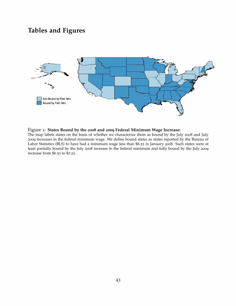
Tables and Figures

Figure 1: States Bound by the 2008 and 2009 Federal Minimum Wage Increase:The map labels states on the basis of whether we characterize them as bound by the July 2008 and July2009 increases in the federal minimum wage. We define bound states as states reported by the Bureau ofLabor Statistics (BLS) to have had a minimum wage less than $6.55 in January 2008. Such states were atleast partially bound by the July 2008 increase in the federal minimum and fully bound by the July 2009

increase from $6.55 to $7.25.

43

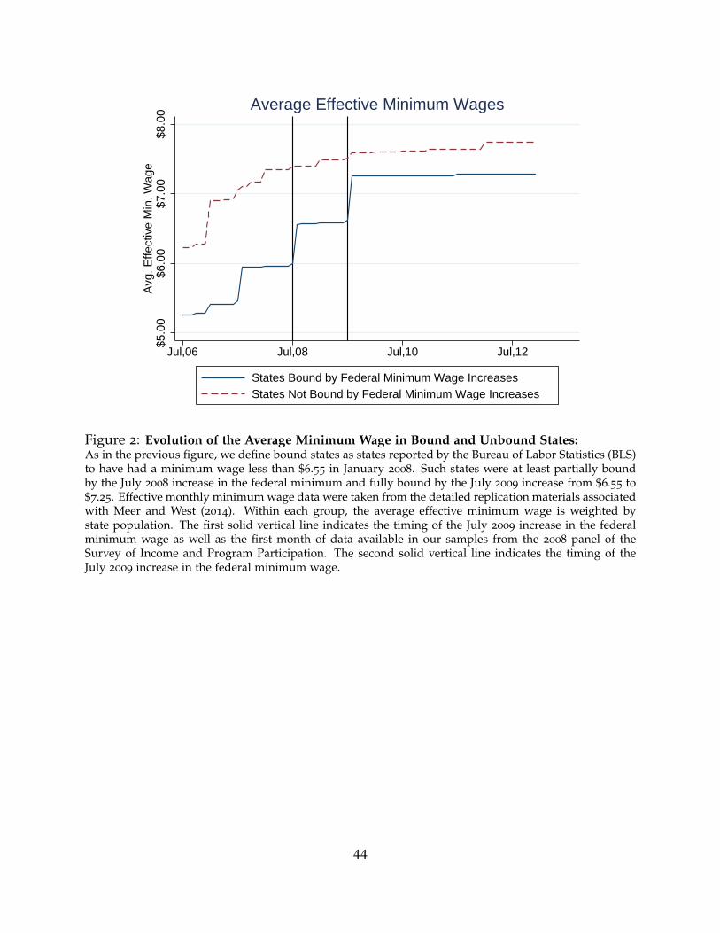
$5.0

0$6

.00

$7.0

0$8

.00

Avg

. Effe

ctiv

e M

in. W

age

Jul,06 Jul,08 Jul,10 Jul,12

States Bound by Federal Minimum Wage IncreasesStates Not Bound by Federal Minimum Wage Increases

Average Effective Minimum Wages

Figure 2: Evolution of the Average Minimum Wage in Bound and Unbound States:As in the previous figure, we define bound states as states reported by the Bureau of Labor Statistics (BLS)to have had a minimum wage less than $6.55 in January 2008. Such states were at least partially boundby the July 2008 increase in the federal minimum and fully bound by the July 2009 increase from $6.55 to$7.25. Effective monthly minimum wage data were taken from the detailed replication materials associatedwith Meer and West (2014). Within each group, the average effective minimum wage is weighted bystate population. The first solid vertical line indicates the timing of the July 2009 increase in the federalminimum wage as well as the first month of data available in our samples from the 2008 panel of theSurvey of Income and Program Participation. The second solid vertical line indicates the timing of theJuly 2009 increase in the federal minimum wage.

44

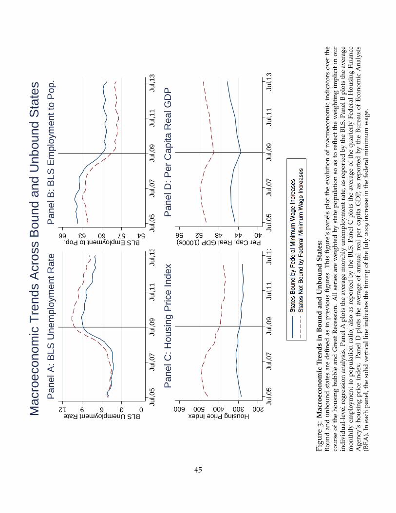
036912BLS Unemployment Rate

Jul,0

5Ju

l,07

Jul,0

9Ju

l,11

Jul,1

3

Pan

el A

: BLS

Une

mpl

oym

ent R

ate

5457606366BLS Employment to Pop.

Jul,0

5Ju

l,07

Jul,0

9Ju

l,11

Jul,1

3

Pan

el B

: BLS

Em

ploy

men

t to

Pop

.

200300400500600Housing Price Index

Jul,0

5Ju

l,07

Jul,0

9Ju

l,11

Jul,1

3

Pan

el C

: Hou

sing

Pric

e In

dex

4044485256Per Cap. Real GDP (1000s)

Jul,0

5Ju

l,07

Jul,0

9Ju

l,11

Jul,1

3

Pan

el D

: Per

Cap

ita R

eal G

DP

Mac

roec

onom

ic T

rend

s A

cros

s B

ound

and

Unb

ound

Sta

tes

Figu

re3

:Mac

roec

onom

icTr

ends

inB

ound

and

Unb

ound

Stat

es:

Boun

dan

dun

boun

dst

ates

are

defin

edas

inpr

evio

usfig

ures

.Th

isfig

ure’

spa

nels

plot

the

evol

utio

nof

mac

roec

onom

icin

dica

tors

over

the

cour

seof

the

hous

ing

bubb

lean

dG

reat

Rec

essi

on.

All

seri

esar

ew

eigh

ted

byst

ate

popu

lati

onso

asto

refle

ctth

ew

eigh

ting

impl

icit

inou

rin

divi

dual

-lev

elre

gres

sion

anal

ysis

.Pan

elA

plot

sth

eav

erag

em

onth

lyun

empl

oym

entr

ate,

asre

port

edby

the

BLS.

Pane

lBpl

ots

the

aver

age

mon

thtl

yem

ploy

men

tto

popu

lati

onra

tio,

also

asre

port

edby

the

BLS.

Pane

lC

plot

sth

eav

erag

eof

the

quar

terl

yFe

dera

lH

ousi

ngFi

nanc

eA

genc

y’s

hous

ing

pric

ein

dex.

Pane

lD

plot

sth

eav

erag

eof

annu

alre

alpe

rca

pita

GD

P,as

repo

rted

byth

eBu

reau

ofEc

onom

icA

naly

sis

(BEA

).In

each

pane

l,th

eso

lidve

rtic

allin

ein

dica

tes

the

tim

ing

ofth

eJu

ly2009

incr

ease

inth

efe

dera

lmin

imum

wag

e.

45

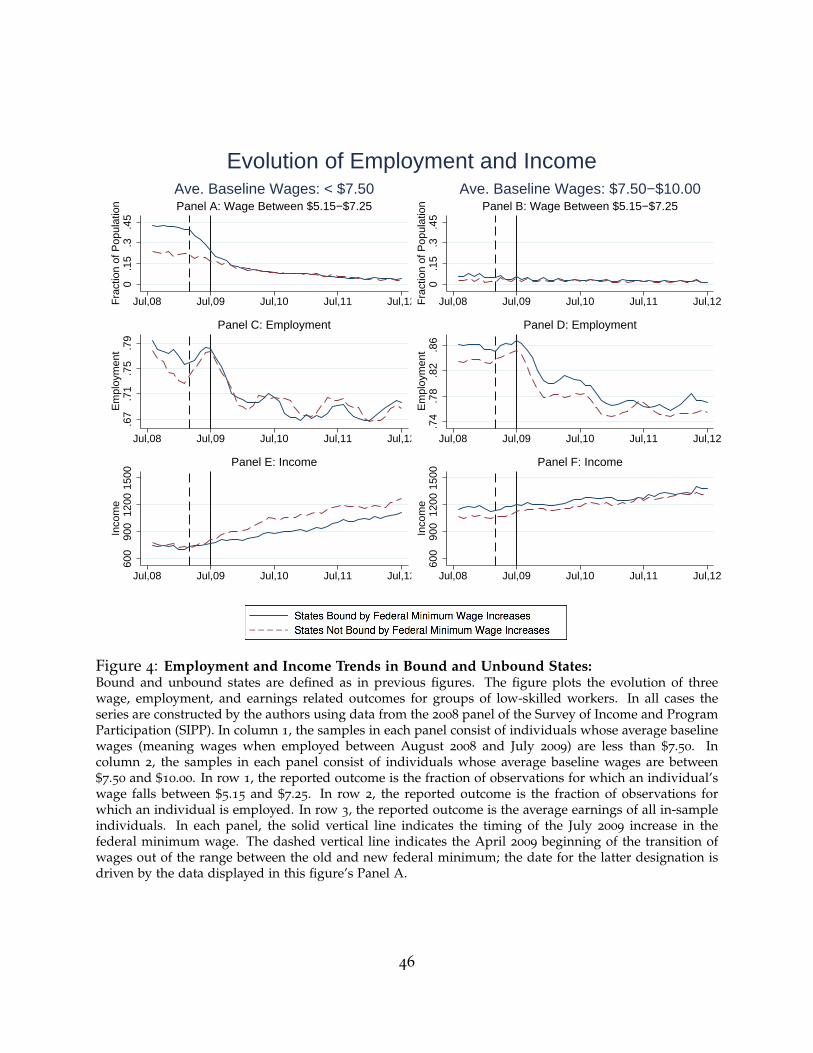
0.1

5.3

.45

Fra

ctio

n of

Pop

ulat

ion

Jul,08 Jul,09 Jul,10 Jul,11 Jul,12

Panel A: Wage Between $5.15−$7.25Ave. Baseline Wages: < $7.50

0.1

5.3

.45

Fra

ctio

n of

Pop

ulat

ion

Jul,08 Jul,09 Jul,10 Jul,11 Jul,12

Panel B: Wage Between $5.15−$7.25Ave. Baseline Wages: $7.50−$10.00

.67

.71

.75

.79

Em

ploy

men

t

Jul,08 Jul,09 Jul,10 Jul,11 Jul,12

Panel C: Employment

.74

.78

.82

.86

Em

ploy

men

t

Jul,08 Jul,09 Jul,10 Jul,11 Jul,12

Panel D: Employment

600

900

1200

1500

Inco

me

Jul,08 Jul,09 Jul,10 Jul,11 Jul,12

Panel E: Income

600

900

1200

1500

Inco

me

Jul,08 Jul,09 Jul,10 Jul,11 Jul,12

Panel F: Income

Evolution of Employment and Income

Figure 4: Employment and Income Trends in Bound and Unbound States:Bound and unbound states are defined as in previous figures. The figure plots the evolution of threewage, employment, and earnings related outcomes for groups of low-skilled workers. In all cases theseries are constructed by the authors using data from the 2008 panel of the Survey of Income and ProgramParticipation (SIPP). In column 1, the samples in each panel consist of individuals whose average baselinewages (meaning wages when employed between August 2008 and July 2009) are less than $7.50. Incolumn 2, the samples in each panel consist of individuals whose average baseline wages are between$7.50 and $10.00. In row 1, the reported outcome is the fraction of observations for which an individual’swage falls between $5.15 and $7.25. In row 2, the reported outcome is the fraction of observations forwhich an individual is employed. In row 3, the reported outcome is the average earnings of all in-sampleindividuals. In each panel, the solid vertical line indicates the timing of the July 2009 increase in thefederal minimum wage. The dashed vertical line indicates the April 2009 beginning of the transition ofwages out of the range between the old and new federal minimum; the date for the latter designation isdriven by the data displayed in this figure’s Panel A.

46

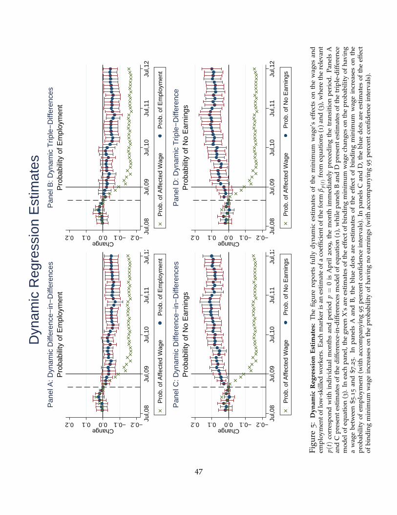
−0.2−0.10.00.10.2Change

Jul,0

8Ju

l,09

Jul,1

0Ju

l,11

Jul,1

2

Pro

b. o

f Affe

cted

Wag

eP

rob.

of E

mpl

oym

ent

Pro

babi

lity

of E

mpl

oym

ent

Pan

el A

: Dyn

amic

Diff

eren

ce−

in−

Diff

eren

ces

−0.2−0.10.00.10.2Change

Jul,0

8Ju

l,09

Jul,1

0Ju

l,11

Jul,1

2

Pro

b. o

f Affe

cted

Wag

eP

rob.

of E

mpl

oym

ent

Pro

babi

lity

of E

mpl

oym

ent

Pan

el B

: Dyn

amic

Trip

le−

Diff

eren

ces

−0.2−0.10.00.10.2Change

Jul,0

8Ju

l,09

Jul,1

0Ju

l,11

Jul,1

2

Pro

b. o

f Affe

cted

Wag

eP

rob.

of N

o E

arni

ngs

Pro

babi

lity

of N

o E

arni

ngs

Pan

el C

: Dyn

amic

Diff

eren

ce−

in−

Diff

eren

ces

−0.2−0.10.00.10.2Change

Jul,0

8Ju

l,09

Jul,1

0Ju

l,11

Jul,1

2

Pro

b. o

f Affe

cted

Wag

eP

rob.

of N

o E

arni

ngs

Pro

babi

lity

of N

o E

arni

ngs

Pan

el D

: Dyn

amic

Trip

le−

Diff

eren

ce

Dyn

amic

Reg

ress

ion

Est

imat

es

Figu

re5

:D

ynam

icR

egre

ssio

nEs

tim

ates

:Th

efig

ure

repo

rts

fully

dyna

mic

esti

mat

esof

the

min

imum

wag

e’s

effe

cts

onth

ew

ages

and

empl

oym

ento

flow

-ski

lled

wor

kers

.Eac

hm

arke

ris

anes

tim

ate

ofa

coef

ficie

ntof

the

form

βp(

t)fr

omeq

uati

ons

(1)a

nd(3

),w

here

the

rele

vant

p(t)

corr

espo

ndw

ith

indi

vidu

alm

onth

san

dpe

riod

p=

0is

Apr

il2009,t

hem

onth

imm

edia

tely

prec

edin

gth

etr

ansi

tion

peri

od.

Pane

lsA

and

Cpr

esen

test

imat

esof

the

diff

eren

ce-i

n-di

ffer

ence

sm

odel

ofeq

uati

on(1

),w

hile

pane

lsB

and

Dpr

esen

test

imat

esof

the

trip

le-d

iffer

ence

mod

elof

equa

tion

(3).

Inea

chpa

nel,

the

gree

nX

’sar

ees

tim

ates

ofth

eef

fect

ofbi

ndin

gm

inim

umw

age

chan

ges

onth

epr

obab

ility

ofha

ving

aw

age

betw

een

$5.1

5an

d$7

.25.

Inpa

nels

Aan

dB,

the

blue

dots

are

esti

mat

esof

the

effe

ctof

bind

ing

min

imum

wag

ein

crea

ses

onth

epr

obab

ility

ofem

ploy

men

t(w

ith

acco

mpa

nyin

g95

perc

ent

confi

denc

ein

terv

als)

.In

pane

lsC

and

D,t

hebl

uedo

tsar

ees

tim

ates

ofth

eef

fect

ofbi

ndin

gm

inim

umw

age

incr

ease

son

the

prob

abili

tyof

havi

ngno

earn

ings

(wit

hac

com

pany

ing

95

perc

ent

confi

denc

ein

terv

als)

.

47

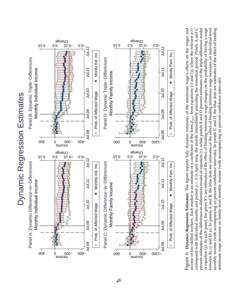
−0.3−0.150.00.15Change

−600−3000300Income

Jul,0

8Ju

l,09

Jul,1

0Ju

l,11

Jul,1

2

Pro

b. o

f Affe

cted

Wag

eM

onth

ly In

d. In

c.

Mon

thly

Indi

vidu

al In

com

eP

anel

A: D

ynam

ic D

iffer

ence

−in

−D

iffer

ence

s

−0.3−0.150.00.15Change

−600−3000300Income

Jul,0

8Ju

l,09

Jul,1

0Ju

l,11

Jul,1

2

Pro

b. o

f Affe

cted

Wag

eM

ontly

Ind.

Inc.

Mon

thly

Indi

vidu

al In

com

eP

anel

B: D

ynam

ic T

riple

−D

iffer

ence

s

−0.3−0.150.00.15Change

−1200−6000600Income

Jul,0

8Ju

l,09

Jul,1

0Ju

l,11

Jul,1

2

Pro

b. o

f Affe

cted

Wag

eM

onth

ly F

am. I

nc.

Mon

thly

Fam

ily In

com

eP

anel

C: D

ynam

ic D

iffer

ence

−in

−D

iffer

ence

s

−0.3−0.150.00.15Change

−1200−6000600Income

Jul,0

8Ju

l,09

Jul,1

0Ju

l,11

Jul,1

2

Pro

b. o

f Affe

cted

Wag

eM

ontly

Fam

. Inc

.

Mon

thly

Fam

ily In

com

eP

anel

D: D

ynam

ic T

riple

−D

iffer

ence

s

Dyn

amic

Reg

ress

ion

Est

imat

es

Figu

re6

:D

ynam

icR

egre

ssio

nEs

tim

ates

:Th

efig

ure

repo

rts

fully

dyna

mic

esti

mat

esof

the

min

imum

wag

e’s

effe

cts

onth

ew

ages

and

inco

me

oflo

w-s

kille

dw

orke

rs.E

ach

mar

ker

isan

esti

mat

eof

aco

effic

ient

ofth

efo

rmβ

p(t)

from

equa

tion

s(1

)and

(3),

whe

reth

ere

leva

ntp(

t)co

rres

pond

wit

hin

divi

dual

mon

ths

and

peri

odp=

0is

Apr

il2009,t

hem

onth

imm

edia

tely

prec

edin

gth

etr

ansi

tion

peri

od.

Pane

lsA

and

Cpr

esen

test

imat

esof

the

diff

eren

ce-i

n-di

ffer

ence

sm

odel

ofeq

uati

on(1

),w

hile

pane

lsB

and

Dpr

esen

test

imat

esof

the

trip

le-d

iffer

ence

mod

elof

equa

tion

(3).

Inea

chpa

nel,

the

gree

nX

’sar

ees

tim

ates

ofth

eef

fect

ofbi

ndin

gm

inim

umw

age

chan

ges

onth

epr

obab

ility

ofha

ving

aw

age

betw

een

$5.1

5an

d$7

.25.

Inpa

nels

Aan

dB,

the

blue

dots

are

esti

mat

esof

the

effe

ctof

bind

ing

min

imum

wag

ein

crea

ses

onin

divi

dual

-lev

elm

onth

lyin

com

e(w

ith

acco

mpa

nyin

g95

perc

ent

confi

denc

ein

terv

als)

.In

pane

lsC

and

D,t

hebl

uedo

tsar

ees

tim

ates

ofth

eef

fect

ofbi

ndin

gm

inim

umw

age

incr

ease

son

fam

ily-l

evel

mon

thly

inco

me

(wit

hac

com

pany

ing

95

perc

ent

confi

denc

ein

terv

als)

.

48

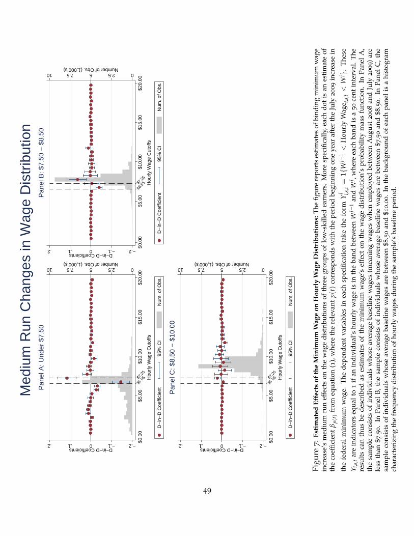
−.2−.10.1.2D−in−D Coefficients

02.557.510Number of Obs. (1,000’s)

$6.5

5$7.2

5

$0.0

0$5

.00

$10.

00$1

5.00

$20.

00

Hou

rly W

age

Cut

offs

D−

in−

D C

oeffi

cien

t95

% C

IN

um. o

f Obs

.

Pan

el A

: Und

er $

7.50

−.2−.10.1.2D−in−D Coefficients

02.557.510Number of Obs. (1,000’s)

$6.5

5$7.2

5

$0.0

0$5

.00

$10.

00$1

5.00

$20.

00

Hou

rly W

age

Cut

offs

D−

in−

D C

oeffi

cien

t95

% C

IN

um. o

f Obs

.

Pan

el B

: $7.

50 −

$8.

50

−.2−.10.1.2D−in−D Coefficients

02.557.510Number of Obs. (1,000’s)

$6.5

5$7.2

5

$0.0

0$5

.00

$10.

00$1

5.00

$20.

00

Hou

rly W

age

Cut

offs

D−

in−

D C

oeffi

cien

t95

% C

IN

um. o

f Obs

.

Pan

el C

: $8.

50 −

$10

.00

Med

ium

Run

Cha

nges

in W

age

Dis

trib

utio

n

Figu

re7:E

stim

ated

Effe

cts

ofth

eM

inim

umW

age

onH

ourl

yW

age

Dis

trib

utio

ns:T

hefig

ure

repo

rts

esti

mat

esof

bind

ing

min

imum

wag

ein

crea

se’s

med

ium

run

effe

cts

onth

ew

age

dist

ribu

tion

sof

thre

egr

oups

oflo

w-s

kille

dea

rner

s.M

ore

spec

ifica

lly,e

ach

dot

isan

esti

mat

eof

the

coef

ficie

ntβ

p(t)

from

equa

tion

(1),

whe

reth

ere

leva

ntp(

t)co

rres

pond

sw

ith

the

peri

odbe

ginn

ing

one

year

afte

rth

eJu

ly2009

incr

ease

in

the

fede

ral

min

imum

wag

e.T

hede

pend

ent

vari

able

sin

each

spec

ifica

tion

take

the

form

Yj i,s

,t=

1{W

j−1<

Hou

rly

Wag

e i,s,t<

Wj }

.Th

ese

Y i,s

,tar

ein

dica

tors

equa

lto

1if

anin

divi

dual

’sho

urly

wag

eis

inth

eba

ndbe

twee

nW

j−1

and

Wj ,w

here

each

band

isa

50

cent

inte

rval

.Th

ere

sult

sca

nth

usbe

desc

ribe

das

esti

mat

esof

the

min

imum

wag

e’s

effe

cton

the

wag

edi

stri

buti

on’s

prob

abili

tym

ass

func

tion

.In

Pane

lA

,th

esa

mpl

eco

nsis

tsof

indi

vidu

als

who

seav

erag

eba

selin

ew

ages

(mea

ning

wag

esw

hen

empl

oyed

betw

een

Aug

ust

2008

and

July

2009)

are

less

than

$7.5

0.

InPa

nel

B,th

esa

mpl

eco

nsis

tsof

indi

vidu

als

who

seav

erag

eba

selin

ew

ages

are

betw

een

$7.5

0an

d$8

.50.

InPa

nel

C,t

hesa

mpl

eco

nsis

tsof

indi

vidu

als

who

seav

erag

eba

selin

ew

ages

are

betw

een

$8.5

0an

d$1

0.0

0.

Inth

eba

ckgr

ound

ofea

chpa

neli

sa

hist

ogra

mch

arac

teri

zing

the

freq

uenc

ydi

stri

buti

onof

hour

lyw

ages

duri

ngth

esa

mpl

e’s

base

line

peri

od.

49

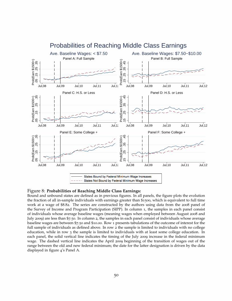
.05

.15

.25

.35

Pro

b(E

arn

$150

0+)

Jul,08 Jul,09 Jul,10 Jul,11 Jul,12

Panel A: Full SampleAve. Baseline Wages: < $7.50

.15

.25

.35

.45

Pro

b(E

arn

$150

0+)

Jul,08 Jul,09 Jul,10 Jul,11 Jul,12

Panel B: Full SampleAve. Baseline Wages: $7.50−$10.00

.05

.15

.25

.35

Pro

b(E

arn

$150

0+)

Jul,08 Jul,09 Jul,10 Jul,11 Jul,12

Panel C: H.S. or Less

.15

.25

.35

.45

Pro

b(E

arn

$150

0+)

Jul,08 Jul,09 Jul,10 Jul,11 Jul,12

Panel D: H.S. or Less

.05

.15

.25

.35

Pro

b(E

arn

$150

0+)

Jul,08 Jul,09 Jul,10 Jul,11 Jul,12

Panel E: Some College +

.15

.25

.35

.45

Pro

b(E

arn

$150

0+)

Jul,08 Jul,09 Jul,10 Jul,11 Jul,12

Panel F: Some College +

Probabilities of Reaching Middle Class Earnings

Figure 8: Probabilities of Reaching Middle Class Earnings:Bound and unbound states are defined as in previous figures. In all panels, the figure plots the evolutionthe fraction of all in-sample individuals with earnings greater than $1500, which is equivalent to full timework at a wage of $8.82. The series are constructed by the authors using data from the 2008 panel ofthe Survey of Income and Program Participation (SIPP). In column 1, the samples in each panel consistof individuals whose average baseline wages (meaning wages when employed between August 2008 andJuly 2009) are less than $7.50. In column 2, the samples in each panel consist of individuals whose averagebaseline wages are between $7.50 and $10.00. Row 1 presents tabulations of the outcome of interest for thefull sample of individuals as defined above. In row 2 the sample is limited to individuals with no collegeeducation, while in row 3 the sample is limited to individuals with at least some college education. Ineach panel, the solid vertical line indicates the timing of the July 2009 increase in the federal minimumwage. The dashed vertical line indicates the April 2009 beginning of the transition of wages out of therange between the old and new federal minimum; the date for the latter designation is driven by the datadisplayed in figure 4’s Panel A.

50

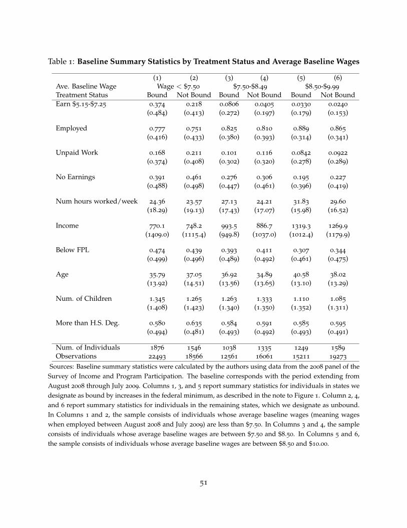
Table 1: Baseline Summary Statistics by Treatment Status and Average Baseline Wages

(1) (2) (3) (4) (5) (6)Ave. Baseline Wage Wage < $7.50 $7.50-$8.49 $8.50-$9.99

Treatment Status Bound Not Bound Bound Not Bound Bound Not BoundEarn $5.15-$7.25 0.374 0.218 0.0806 0.0405 0.0330 0.0240

(0.484) (0.413) (0.272) (0.197) (0.179) (0.153)

Employed 0.777 0.751 0.825 0.810 0.889 0.865

(0.416) (0.433) (0.380) (0.393) (0.314) (0.341)

Unpaid Work 0.168 0.211 0.101 0.116 0.0842 0.0922

(0.374) (0.408) (0.302) (0.320) (0.278) (0.289)

No Earnings 0.391 0.461 0.276 0.306 0.195 0.227

(0.488) (0.498) (0.447) (0.461) (0.396) (0.419)

Num hours worked/week 24.36 23.57 27.13 24.21 31.83 29.60

(18.29) (19.13) (17.43) (17.07) (15.98) (16.52)

Income 770.1 748.2 993.5 886.7 1319.3 1269.9(1409.0) (1115.4) (949.8) (1037.0) (1012.4) (1179.9)

Below FPL 0.474 0.439 0.393 0.411 0.307 0.344

(0.499) (0.496) (0.489) (0.492) (0.461) (0.475)

Age 35.79 37.05 36.92 34.89 40.58 38.02

(13.92) (14.51) (13.56) (13.65) (13.10) (13.29)

Num. of Children 1.345 1.265 1.263 1.333 1.110 1.085

(1.408) (1.423) (1.340) (1.350) (1.352) (1.311)

More than H.S. Deg. 0.580 0.635 0.584 0.591 0.585 0.595

(0.494) (0.481) (0.493) (0.492) (0.493) (0.491)

Num. of Individuals 1876 1546 1038 1335 1249 1589

Observations 22493 18566 12561 16061 15211 19273

Sources: Baseline summary statistics were calculated by the authors using data from the 2008 panel of theSurvey of Income and Program Participation. The baseline corresponds with the period extending fromAugust 2008 through July 2009. Columns 1, 3, and 5 report summary statistics for individuals in states wedesignate as bound by increases in the federal minimum, as described in the note to Figure 1. Column 2, 4,and 6 report summary statistics for individuals in the remaining states, which we designate as unbound.In Columns 1 and 2, the sample consists of individuals whose average baseline wages (meaning wageswhen employed between August 2008 and July 2009) are less than $7.50. In Columns 3 and 4, the sampleconsists of individuals whose average baseline wages are between $7.50 and $8.50. In Columns 5 and 6,the sample consists of individuals whose average baseline wages are between $8.50 and $10.00.

51

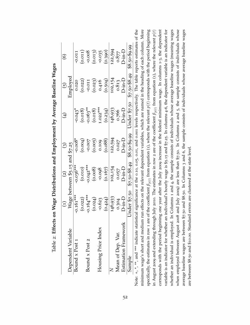
Tabl

e2:E

ffec

tson

Wag

eD

istr

ibut

ions

and

Empl

oym

ent

byA

vera

geB

asel

ine

Wag

es

(1)

(2)

(3)

(4)

(5)

(6)

Dep

ende

ntV

aria

ble

Wag

ebe

twee

n$5

.15

and

$7.2

5Em

ploy

edBo

und

xPo

st1

-0.1

61**

*-0

.036**

*-0

.008*

-0.0

43*

0.0

20

-0.0

11

(0.0

22)

(0.0

10)

(0.0

04)

(0.0

18)

(0.0

22)

(0.0

11)

Boun

dx

Post

2-0

.164**

*-0

.042**

*-0

.007

-0.0

63**

-0.0

11

-0.0

08

(0.0

24)

(0.0

08)

(0.0

05)

(0.0

18)

(0.0

23)

(0.0

13)

Hou

sing

Pric

eIn

dex

-0.6

23

-0.0

98

0.1

09

1.0

22**

*0.4

16

-0.0

35

(0.4

24)

(0.1

67)

(0.0

88)

(0.2

34)

(0.5

04)

(0.3

90)

N146,9

33

102

,154

122,5

94

146,9

33

102,1

54

122,5

94

Mea

nof

Dep

.Var

.0.3

04

0.0

57

0.0

27

0.7

66

0.8

13

0.8

77

Esti

mat

ion

Fram

ewor

kD

-in-

DD

-in-

DD

-in-

DD

-in-

DD

-in-

DD

-in-

DSa

mpl

eU

nder

$7.5

0$7

.50-$

8.4

9$8

.50-$

9.9

9U

nder

$7.5

0$7

.50-$

8.4

9$8

.50-$

9.9

9

Not

e:+,

*,**

,an

d**

*in

dica

test

atis

tica

lsi

gnifi

canc

eat

the

0.1

0,

0.0

5,

0.0

1,

and

0.0

01

leve

lsre

spec

tive

ly.

The

tabl

ere

port

ses

tim

ates

ofth

em

inim

umw

age’

ssh

ort

and

med

ium

run

effe

cts

onth

ere

leva

ntde

pend

ent

vari

able

s,w

hich

are

nam

edin

the

head

ing

ofea

chco

lum

n.M

ore

spec

ifica

lly,t

hees

tim

ates

inro

w1

are

ofth

eco

effic

ient

βp(

t)fr

omeq

uati

on(1

),w

here

the

rele

vant

p(t)

corr

espo

nds

wit

hth

epe

riod

begi

nnin

gin

Aug

ust2

009

and

exte

ndin

gth

roug

hJu

ly2010.T

hees

tim

ates

inro

w2

are

ofth

eco

effic

ient

βp(

t)fr

omeq

uati

on(1

),w

here

the

rele

vant

p(t)

corr

espo

nds

wit

hth

epe

riod

begi

nnin

gon

eye

araf

ter

the

July

2009

incr

ease

inth

efe

dera

lm

inim

umw

age.

Inco

lum

ns1-3

,the

depe

nden

tva

riab

leis

anin

dica

tor

for

whe

ther

anin

divi

dual

’sho

urly

wag

eis

$5.1

5an

d$7

.25.I

nco

lum

ns4-6

,the

depe

nden

tvar

iabl

eis

anin

dica

tor

for

whe

ther

anin

divi

dual

isem

ploy

ed.

InC

olum

ns1

and

4,t

hesa

mpl

eco

nsis

tsof

indi

vidu

als

who

seav

erag

eba

selin

ew

ages

(mea

ning

wag

esw

hen

empl

oyed

betw

een

Aug

ust

2008

and

July

2009)

are

less

than

$7.5

0.

InC

olum

ns2

and

5,

the

sam

ple

cons

ists

ofin

divi

dual

sw

hose

aver

age

base

line

wag

esar

ebe

twee

n$7

.50

and

$8.5

0.

InC

olum

ns3

and

6,t

hesa

mpl

eco

nsis

tsof

indi

vidu

als

who

seav

erag

eba

selin

ew

ages

are

betw

een

$8.5

0an

d$1

0.0

0.S

tand

ard

erro

rsar

ecl

uste

red

atth

est

ate

leve

l.

52

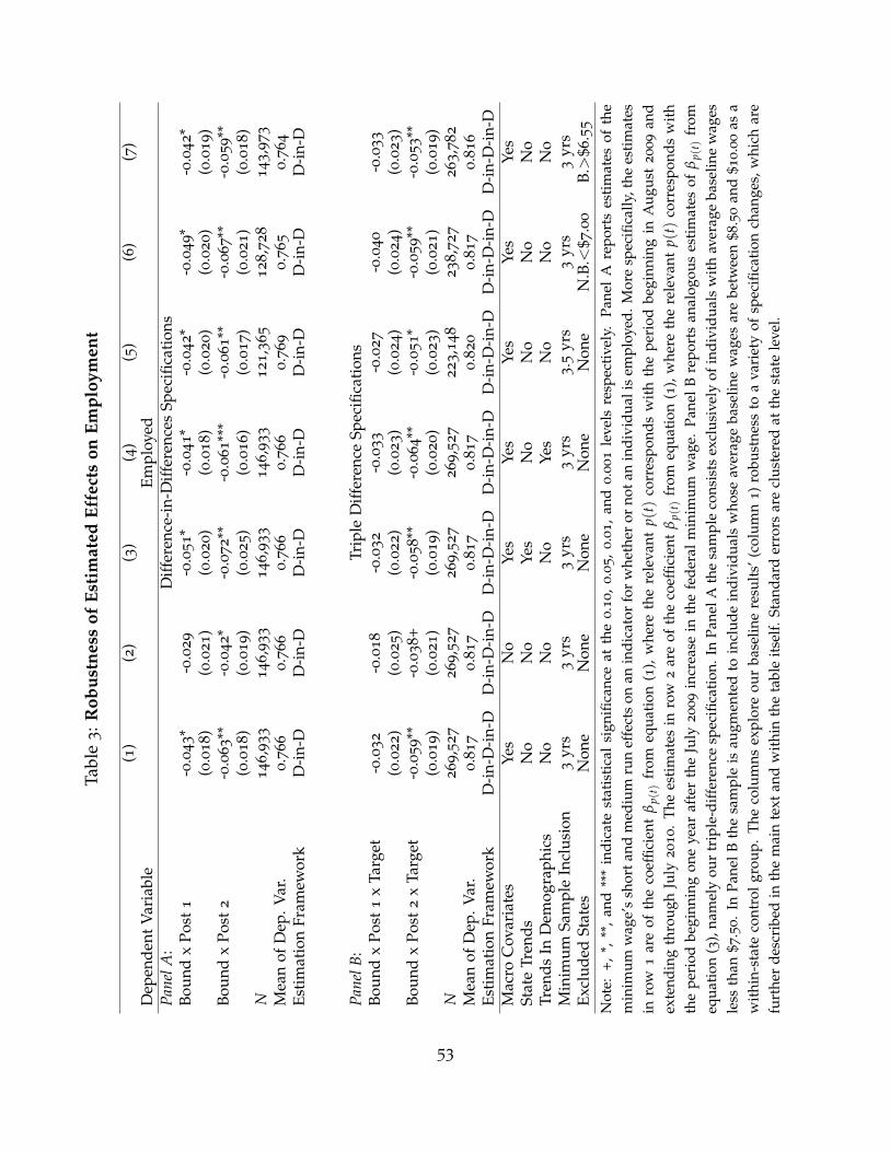
Tabl

e3

:Rob

ustn

ess

ofEs

tim

ated

Effe

cts

onEm

ploy

men

t

(1)

(2)

(3)

(4)

(5)

(6)

(7)

Dep

ende

ntV

aria

ble

Empl

oyed

Pane

lA:

Diff

eren

ce-i

n-D

iffer

ence

sSp

ecifi

cati

ons

Boun

dx

Post

1-0

.043*

-0.0

29

-0.0

51*

-0.0

41*

-0.0

42*

-0.0

49*

-0.0

42*

(0.0

18)

(0.0

21)

(0.0

20)

(0.0

18)

(0.0

20)

(0.0

20)

(0.0

19)

Boun

dx

Post

2-0

.063**

-0.0

42*

-0.0

72**

-0.0

61**

*-0

.061**

-0.0

67**

-0.0

59**

(0.0

18)

(0.0

19)

(0.0

25)

(0.0

16)

(0.0

17)

(0.0

21)

(0.0

18)

N146,9

33

146,9

33

146,9

33

146,9

33

121,3

65

128,7

28

143,9

73

Mea

nof

Dep

.Var

.0.7

66

0.7

66

0.7

66

0.7

66

0.7

69

0.7

65

0.7

64

Esti

mat

ion

Fram

ewor

kD

-in-

DD

-in-

DD

-in-

DD

-in-

DD

-in-

DD

-in-

DD

-in-

D

Pane

lB:

Trip

leD

iffer

ence

Spec

ifica

tion

sBo

und

xPo

st1

xTa

rget

-0.0

32

-0.0

18

-0.0

32

-0.0

33

-0.0

27

-0.0

40

-0.0

33

(0.0

22)

(0.0

25)

(0.0

22)

(0.0

23)

(0.0

24)

(0.0

24)

(0.0

23)

Boun

dx

Post

2x

Targ

et-0

.059**

-0.0

38+

-0.0

58**

-0.0

64**

-0.0

51*

-0.0

59**

-0.0

53**

(0.0

19)

(0.0

21)

(0.0

19)

(0.0

20)

(0.0

23)

(0.0

21)

(0.0

19)

N269,5

27

269,5

27

269,5

27

269,5

27

223,1

48

238,7

27

263,7

82

Mea

nof

Dep

.Var

.0.8

17

0.8

17

0.8

17

0.8

17

0.8

20

0.8

17

0.8

16

Esti

mat

ion

Fram

ewor

kD

-in-

D-i

n-D

D-i

n-D

-in-

DD

-in-

D-i

n-D

D-i

n-D

-in-

DD

-in-

D-i

n-D

D-i

n-D

-in-

DD

-in-

D-i

n-D

Mac

roC

ovar

iate

sYe

sN

oYe

sYe

sYe

sYe

sYe

sSt

ate

Tren

dsN

oN

oYe

sN

oN

oN

oN

oTr

ends

InD

emog

raph

ics

No

No

No

Yes

No

No

No

Min

imum

Sam

ple

Incl

usio

n3

yrs

3yr

s3

yrs

3yr

s3.5

yrs

3yr

s3

yrs

Excl

uded

Stat

esN

one

Non

eN

one

Non

eN

one

N.B

.<$7

.00

B.>

$6.5

5

Not

e:+,

*,**

,an

d**

*in

dica

test

atis

tica

lsi

gnifi

canc

eat

the

0.1

0,

0.0

5,

0.0

1,

and

0.0

01

leve

lsre

spec

tive

ly.

Pane

lA

repo

rts

esti

mat

esof

the

min

imum

wag

e’s

shor

tand

med

ium

run

effe

cts

onan

indi

cato

rfo

rw

heth

eror

nota

nin

divi

dual

isem

ploy

ed.M

ore

spec

ifica

lly,t

hees

tim

ates

inro

w1

are

ofth

eco

effic

ient

βp(

t)fr

omeq

uati

on(1

),w

here

the

rele

vant

p(t)

corr

espo

nds

wit

hth

epe

riod

begi

nnin

gin

Aug

ust

2009

and

exte

ndin

gth

roug

hJu

ly2010.

The

esti

mat

esin

row

2ar

eof

the

coef

ficie

ntβ

p(t)

from

equa

tion

(1),

whe

reth

ere

leva

ntp(

t)co

rres

pond

sw

ith

the

peri

odbe

ginn

ing

one

year

afte

rth

eJu

ly2009

incr

ease

inth

efe

dera

lm

inim

umw

age.

Pane

lB

repo

rts

anal

ogou

ses

tim

ates

ofβ

p(t)

from

equa

tion

(3),

nam

ely

our

trip

le-d

iffer

ence

spec

ifica

tion

.In

Pane

lAth

esa

mpl

eco

nsis

tsex

clus

ivel

yof

indi

vidu

als

wit

hav

erag

eba

selin

ew

ages

less

than

$7.5

0.

InPa

nelB

the

sam

ple

isau

gmen

ted

toin

clud

ein

divi

dual

sw

hose

aver

age

base

line

wag

esar

ebe

twee

n$8

.50

and

$10.0

0as

aw

ithi

n-st

ate

cont

rolg

roup

.Th

eco

lum

nsex

plor

eou

rba

selin

ere

sult

s’(c

olum

n1)

robu

stne

ssto

ava

riet

yof

spec

ifica

tion

chan

ges,

whi

char

efu

rthe

rde

scri

bed

inth

em

ain

text

and

wit

hin

the

tabl

eit

self

.Sta

ndar

der

rors

are

clus

tere

dat

the

stat

ele

vel.

53

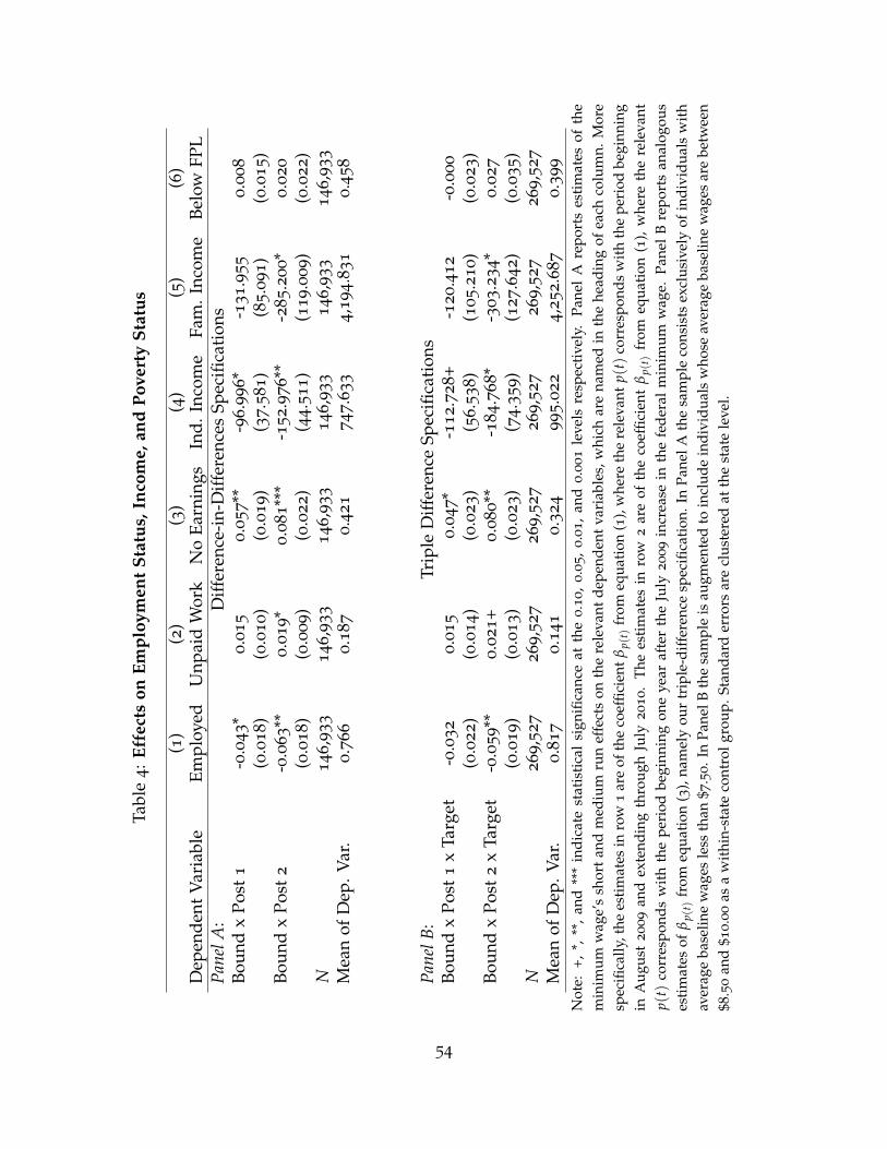
Tabl

e4:E

ffec

tson

Empl

oym

ent

Stat

us,I

ncom

e,an

dPo

vert

ySt

atus

(1)

(2)

(3)

(4)

(5)

(6)

Dep

ende

ntV

aria

ble

Empl

oyed

Unp

aid

Wor

kN

oEa

rnin

gsIn

d.In

com

eFa

m.I

ncom

eBe

low

FPL

Pane

lA:

Diff

eren

ce-i

n-D

iffer

ence

sSp

ecifi

cati

ons

Boun

dx

Post

1-0

.043*

0.0

15

0.0

57**

-96.9

96*

-131.9

55

0.0

08

(0.0

18)

(0.0

10)

(0.0

19)

(37.5

81)

(85.0

91)

(0.0

15)

Boun

dx

Post

2-0

.063**

0.0

19*

0.0

81**

*-1

52.9

76**

-285.2

00*

0.0

20

(0.0

18)

(0.0

09)

(0.0

22)

(44.5

11)

(119.0

09)

(0.0

22)

N146,9

33

146,9

33

146,9

33

146,9

33

146,9

33

146,9

33

Mea

nof

Dep

.Var

.0.7

66

0.1

87

0.4

21

747.6

33

4,1

94.8

31

0.4

58

Pane

lB:

Trip

leD

iffer

ence

Spec

ifica

tion

sBo

und

xPo

st1

xTa

rget

-0.0

32

0.0

15

0.0

47*

-112.7

28+

-120.4

12

-0.0

00

(0.0

22)

(0.0

14)

(0.0

23)

(56.5

38)

(105.2

10)

(0.0

23)

Boun

dx

Post

2x

Targ

et-0

.059**

0.0

21+

0.0

80**

-184.7

68*

-303.2

34*

0.0

27

(0.0

19)

(0.0

13)

(0.0

23)

(74.3

59)

(127.6

42)

(0.0

35)

N269,5

27

269,5

27

269,5

27

269,5

27

269,5

27

269,5

27

Mea

nof

Dep

.Var

.0.8

17

0.1

41

0.3

24

995.0

22

4,2

52.6

87

0.3

99

Not

e:+,

*,**

,an

d**

*in

dica

test

atis

tica

lsi

gnifi

canc

eat

the

0.1

0,

0.0

5,

0.0

1,

and

0.0

01

leve

lsre

spec

tive

ly.

Pane

lA

repo

rts

esti

mat

esof

the

min

imum

wag

e’s

shor

tan

dm

ediu

mru

nef

fect

son

the

rele

vant

depe

nden

tva

riab

les,

whi

char

ena

med

inth

ehe

adin

gof

each

colu

mn.

Mor

esp

ecifi

cally

,the

esti

mat

esin

row

1ar

eof

the

coef

ficie

ntβ

p(t)

from

equa

tion

(1),

whe

reth

ere

leva

ntp(

t)co

rres

pond

sw

ith

the

peri

odbe

ginn

ing

inA

ugus

t2009

and

exte

ndin

gth

roug

hJu

ly2010.

The

esti

mat

esin

row

2ar

eof

the

coef

ficie

ntβ

p(t)

from

equa

tion

(1),

whe

reth

ere

leva

ntp(

t)co

rres

pond

sw

ith

the

peri

odbe

ginn

ing

one

year

afte

rth

eJu

ly2009

incr

ease

inth

efe

dera

lm

inim

umw

age.

Pane

lB

repo

rts

anal

ogou

ses

tim

ates

ofβ

p(t)

from

equa

tion

(3),

nam

ely

our

trip

le-d

iffer

ence

spec

ifica

tion

.In

Pane

lAth

esa

mpl

eco

nsis

tsex

clus

ivel

yof

indi

vidu

als

wit

hav

erag

eba

selin

ew

ages

less

than

$7.5

0.I

nPa

nelB

the

sam

ple

isau

gmen

ted

toin

clud

ein

divi

dual

sw

hose

aver

age

base

line

wag

esar

ebe

twee

n$8

.50

and

$10.0

0as

aw

ithi

n-st

ate

cont

rolg

roup

.Sta

ndar

der

rors

are

clus

tere

dat

the

stat

ele

vel.

54

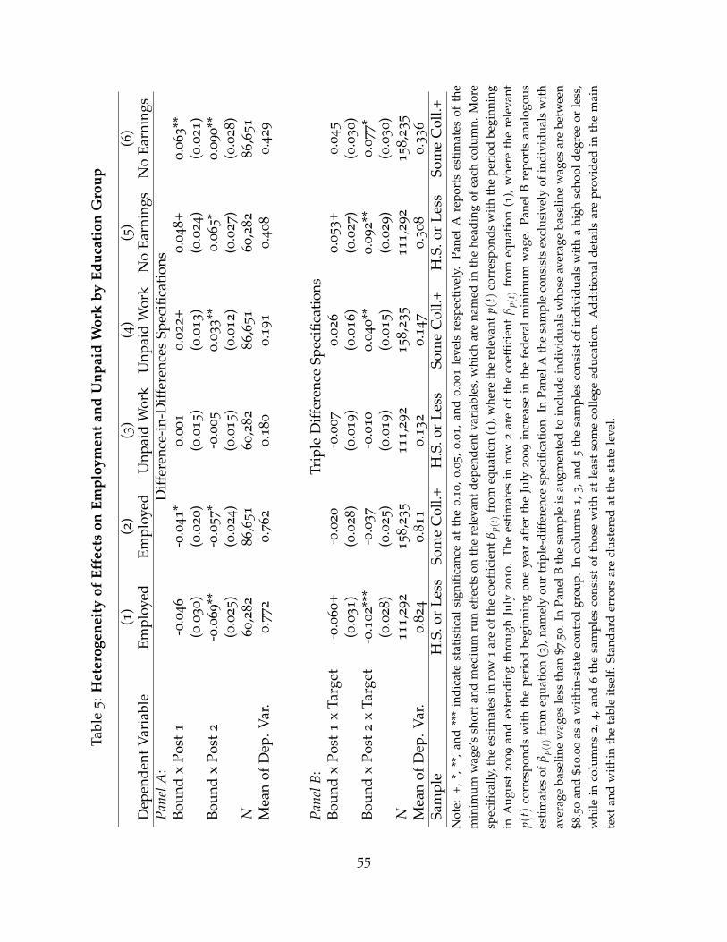
Tabl

e5:H

eter

ogen

eity

ofEf

fect

son

Empl

oym

ent

and

Unp

aid

Wor

kby

Educ

atio

nG

roup

(1)

(2)

(3)

(4)

(5)

(6)

Dep

ende

ntV

aria

ble

Empl

oyed

Empl

oyed

Unp

aid

Wor

kU

npai

dW

ork

No

Earn

ings

No

Earn

ings

Pane

lA:

Diff

eren

ce-i

n-D

iffer

ence

sSp

ecifi

cati

ons

Boun

dx

Post

1-0

.046

-0.0

41*

0.0

01

0.0

22+

0.0

48+

0.0

63**

(0.0

30)

(0.0

20)

(0.0

15)

(0.0

13)

(0.0

24)

(0.0

21)

Boun

dx

Post

2-0

.069**

-0.0

57*

-0.0

05

0.0

33**

0.0

65*

0.0

90**

(0.0

25)

(0.0

24)

(0.0

15)

(0.0

12)

(0.0

27)

(0.0

28)

N60,2

82

86,6

51

60,2

82

86,6

51

60,2

82

86,6

51

Mea

nof

Dep

.Var

.0.7

72

0.7

62

0.1

80

0.1

91

0.4

08

0.4

29

Pane

lB:

Trip

leD

iffer

ence

Spec

ifica

tion

sBo

und

xPo

st1

xTa

rget

-0.0

60+

-0.0

20

-0.0

07

0.0

26

0.0

53+

0.0

45

(0.0

31)

(0.0

28)

(0.0

19)

(0.0

16)

(0.0

27)

(0.0

30)

Boun

dx

Post

2x

Targ

et-0

.102**

*-0

.037

-0.0

10

0.0

40**

0.0

92**

0.0

77*

(0.0

28)

(0.0

25)

(0.0

19)

(0.0

15)

(0.0

29)

(0.0

30)

N111,2

92

158,2

35

111,2

92

158,2

35

111,2

92

158,2

35

Mea

nof

Dep

.Var

.0.8

24

0.8

11

0.1

32

0.1

47

0.3

08

0.3

36

Sam

ple

H.S

.or

Less

Som

eC

oll.+

H.S

.or

Less

Som

eC

oll.+

H.S

.or

Less

Som

eC

oll.+

Not

e:+,

*,**

,an

d**

*in

dica

test

atis

tica

lsi

gnifi

canc

eat

the

0.1

0,

0.0

5,

0.0

1,

and

0.0

01

leve

lsre

spec

tive

ly.

Pane

lA

repo

rts

esti

mat

esof

the

min

imum

wag

e’s

shor

tan

dm

ediu

mru

nef

fect

son

the

rele

vant

depe

nden

tva

riab

les,

whi

char

ena

med

inth

ehe

adin

gof

each

colu

mn.

Mor

esp

ecifi

cally

,the

esti

mat

esin

row

1ar

eof

the

coef

ficie

ntβ

p(t)

from

equa

tion

(1),

whe

reth

ere

leva

ntp(

t)co

rres

pond

sw

ith

the

peri

odbe

ginn

ing

inA

ugus

t2009

and

exte

ndin

gth

roug

hJu

ly2010.

The

esti

mat

esin

row

2ar

eof

the

coef

ficie

ntβ

p(t)

from

equa

tion

(1),

whe

reth

ere

leva

ntp(

t)co

rres

pond

sw

ith

the

peri

odbe

ginn

ing

one

year

afte

rth

eJu

ly2009

incr

ease

inth

efe

dera

lm

inim

umw

age.

Pane

lB

repo

rts

anal

ogou

ses

tim

ates

ofβ

p(t)

from

equa

tion

(3),

nam

ely

our

trip

le-d

iffer

ence

spec

ifica

tion

.In

Pane

lAth

esa

mpl

eco

nsis

tsex

clus

ivel

yof

indi

vidu

als

wit

hav

erag

eba

selin

ew

ages

less

than

$7.5

0.I

nPa

nelB

the

sam

ple

isau

gmen

ted

toin

clud

ein

divi

dual

sw

hose

aver

age

base

line

wag

esar

ebe

twee

n$8

.50

and

$10.0

0as

aw

ithi

n-st

ate

cont

rolg

roup

.In

colu

mns

1,3

,and

5th

esa

mpl

esco

nsis

tof

indi

vidu

als

wit

ha

high

scho

olde

gree

orle

ss,

whi

lein

colu

mns

2,4

,and

6th

esa

mpl

esco

nsis

tof

thos

ew

ith

atle

ast

som

eco

llege

educ

atio

n.A

ddit

iona

lde

tails

are

prov

ided

inth

em

ain

text

and

wit

hin

the

tabl

eit

self

.Sta

ndar

der

rors

are

clus

tere

dat

the

stat

ele

vel.

55

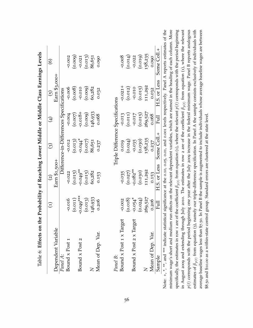
Tabl

e6:E

ffec

tson

the

Prob

abil

ity

ofR

each

ing

Low

erM

iddl

eor

Mid

dle

Cla

ssEa

rnin

gsLe

vels

(1)

(2)

(3)

(4)

(5)

(6)

Dep

ende

ntV

aria

ble

Earn

$1,5

00+

Earn

$3,0

00+

Pane

lA:

Diff

eren

ce-i

n-D

iffer

ence

sSp

ecifi

cati

ons

Boun

dx

Post

1-0

.016

-0.0

22

-0.0

12

-0.0

04

-0.0

06

-0.0

02

(0.0

11)

(0.0

15)

(0.0

13)

(0.0

07)

(0.0

08)

(0.0

09)

Boun

dx

Post

2-0

.049**

*-0

.049**

-0.0

44*

-0.0

18+

-0.0

10

-0.0

21

(0.0

13)

(0.0

15)

(0.0

17)

(0.0

09)

(0.0

09)

(0.0

13)

N146,9

33

60,2

82

86,6

51

146,9

33

60,2

82

86,6

51

Mea

nof

Dep

.Var

.0.2

06

0.1

53

0.2

37

0.0

68

0.0

32

0.0

90

Pane

lB:

Trip

leD

iffer

ence

Spec

ifica

tion

sBo

und

xPo

st1

xTa

rget

-0.0

02

-0.0

35

0.0

19

-0.0

13

-0.0

21+

-0.0

08

(0.0

18)

(0.0

27)

(0.0

24)

(0.0

11)

(0.0

12)

(0.0

14)

Boun

dx

Post

2x

Targ

et-0

.054*

-0.0

82**

-0.0

35

-0.0

17

-0.0

10

-0.0

22

(0.0

24)

(0.0

30)

(0.0

30)

(0.0

15)

(0.0

15)

(0.0

19)

N269,5

27

111,2

92

158,2

35

269,5

27

111,2

92

158,2

35

Mea

nof

Dep

.Var

.0.2

06

0.1

53

0.2

37

0.0

68

0.0

32

0.0

90

Sam

ple

Full

H.S

.or

Less

Som

eC

oll.+

Full

H.S

.or

Less

Som

eC

oll.+

Not

e:+,

*,**

,an

d**

*in

dica

test

atis

tica

lsi

gnifi

canc

eat

the

0.1

0,

0.0

5,

0.0

1,

and

0.0

01

leve

lsre

spec

tive

ly.

Pane

lA

repo

rts

esti

mat

esof

the

min

imum

wag

e’s

shor

tan

dm

ediu

mru

nef

fect

son

the

rele

vant

depe

nden

tva

riab

les,

whi

char

ena

med

inth

ehe

adin

gof

each

colu

mn.

Mor

esp

ecifi

cally

,the

esti

mat

esin

row

1ar

eof

the

coef

ficie

ntβ

p(t)

from

equa

tion

(1),

whe

reth

ere

leva

ntp(

t)co

rres

pond

sw

ith

the

peri

odbe

ginn

ing

inA

ugus

t2009

and

exte

ndin

gth

roug

hJu

ly2010.

The

esti

mat

esin

row

2ar

eof

the

coef

ficie

ntβ

p(t)

from

equa

tion

(1),

whe

reth

ere

leva

ntp(

t)co

rres

pond

sw

ith

the

peri

odbe

ginn

ing

one

year

afte

rth

eJu

ly2009

incr

ease

inth

efe

dera

lm

inim

umw

age.

Pane

lB

repo

rts

anal

ogou

ses

tim

ates

ofβ

p(t)

from

equa

tion

(3),

nam

ely

our

trip

le-d

iffer

ence

spec

ifica

tion

.In

Pane

lAth

esa

mpl

eco

nsis

tsex

clus

ivel

yof

indi

vidu

als

wit

hav

erag

eba

selin

ew

ages

less

than

$7.5

0.I

nPa

nelB

the

sam

ple

isau

gmen

ted

toin

clud

ein

divi

dual

sw

hose

aver

age

base

line

wag

esar

ebe

twee

n$8

.50

and

$10.0

0as

aw

ithi

n-st

ate

cont

rolg

roup

.Sta

ndar

der

rors

are

clus

tere

dat

the

stat

ele

vel.

56

Appendix (Intended For Online Publication Only)

57

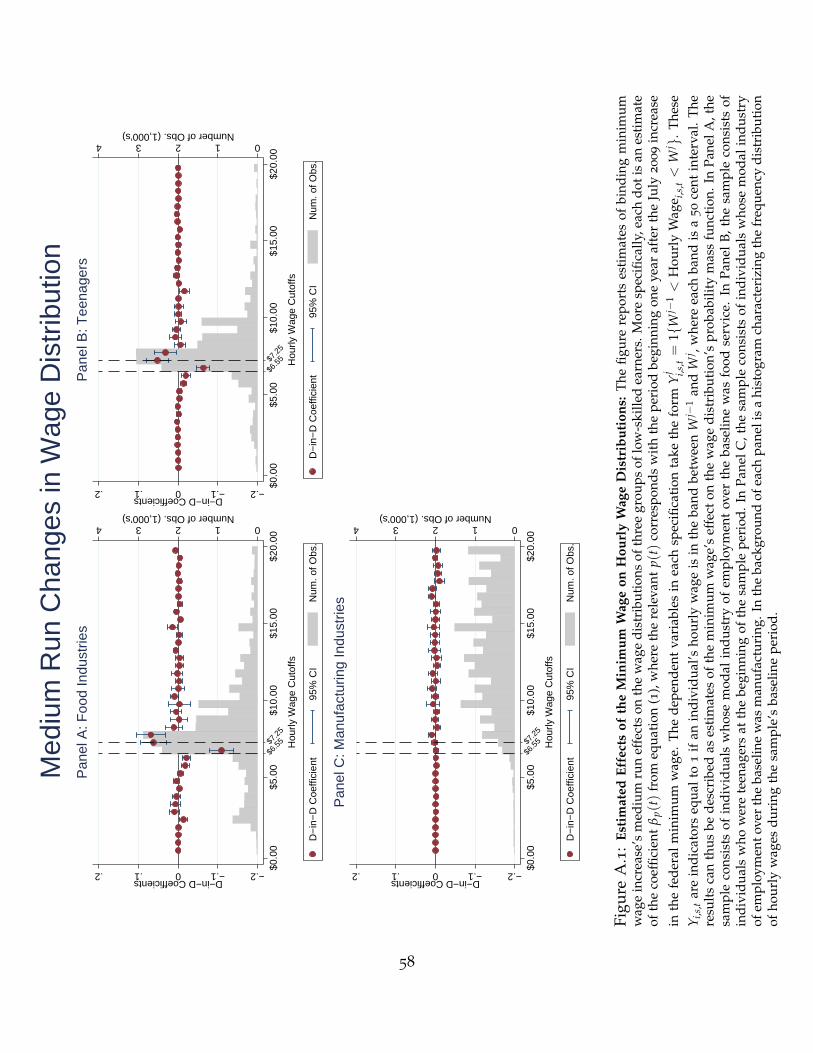
−.2−.10.1.2D−in−D Coefficients

01234Number of Obs. (1,000’s)

$6.5

5$7.2

5

$0.0

0$5

.00

$10.

00$1

5.00

$20.

00

Hou

rly W

age

Cut

offs

D−

in−

D C

oeffi

cien

t95

% C

IN

um. o

f Obs

.

Pan

el A

: Foo

d In

dust

ries

−.2−.10.1.2D−in−D Coefficients

01234Number of Obs. (1,000’s)

$6.5

5$7.2

5

$0.0

0$5

.00

$10.

00$1

5.00

$20.

00

Hou

rly W

age

Cut

offs

D−

in−

D C

oeffi

cien

t95

% C

IN

um. o

f Obs

.

Pan

el B

: Tee

nage

rs

−.2−.10.1.2D−in−D Coefficients

01234Number of Obs. (1,000’s)

$6.5

5$7.2

5

$0.0

0$5

.00

$10.

00$1

5.00

$20.

00

Hou

rly W

age

Cut

offs

D−

in−

D C

oeffi

cien

t95

% C

IN

um. o

f Obs

.

Pan

el C

: Man

ufac

turin

g In

dust

ries

Med

ium

Run

Cha

nges

in W

age

Dis

trib

utio

n

Figu

reA

.1:

Esti

mat

edEf

fect

sof

the

Min

imum

Wag

eon

Hou

rly

Wag

eD

istr

ibut

ions

:Th

efig

ure

repo

rts

esti

mat

esof

bind

ing

min

imum

wag

ein

crea

se’s

med

ium

run

effe

cts

onth

ew

age

dist

ribu

tion

sof

thre

egr

oups

oflo

w-s

kille

dea

rner

s.M

ore

spec

ifica

lly,e

ach

doti

san

esti

mat

eof

the

coef

ficie

ntβ

p(t)

from

equa

tion

(1),

whe

reth

ere

leva

ntp(

t)co

rres

pond

sw

ith

the

peri

odbe

ginn

ing

one

year

afte

rth

eJu

ly2009

incr

ease

inth

efe

dera

lmin

imum

wag

e.Th

ede

pend

ent

vari

able

sin

each

spec

ifica

tion

take

the

form

Yj i,s

,t=

1{W

j−1<

Hou

rly

Wag

e i,s,t<

Wj }

.Th

ese

Y i,s

,tar

ein

dica

tors

equa

lto

1if

anin

divi

dual

’sho

urly

wag

eis

inth

eba

ndbe

twee

nW

j−1

and

Wj ,w

here

each

band

isa

50

cent

inte

rval

.Th

ere

sult

sca

nth

usbe

desc

ribe

das

esti

mat

esof

the

min

imum

wag

e’s

effe

cton

the

wag

edi

stri

buti

on’s

prob

abili

tym

ass

func

tion

.In

Pane

lA,t

hesa

mpl

eco

nsis

tsof

indi

vidu

als

who

sem

odal

indu

stry

ofem

ploy

men

tov

erth

eba

selin

ew

asfo

odse

rvic

e.In

Pane

lB,

the

sam

ple

cons

ists

ofin

divi

dual

sw

how

ere

teen

ager

sat

the

begi

nnin

gof

the

sam

ple

peri

od.

InPa

nelC

,the

sam

ple

cons

ists

ofin

divi

dual

sw

hose

mod

alin

dust

ryof

empl

oym

ento

ver

the

base

line

was

man

ufac

turi

ng.I

nth

eba

ckgr

ound

ofea

chpa

neli

sa

hist

ogra

mch

arac

teri

zing

the

freq

uenc

ydi

stri

buti

onof

hour

lyw

ages

duri

ngth

esa

mpl

e’s

base

line

peri

od.

58

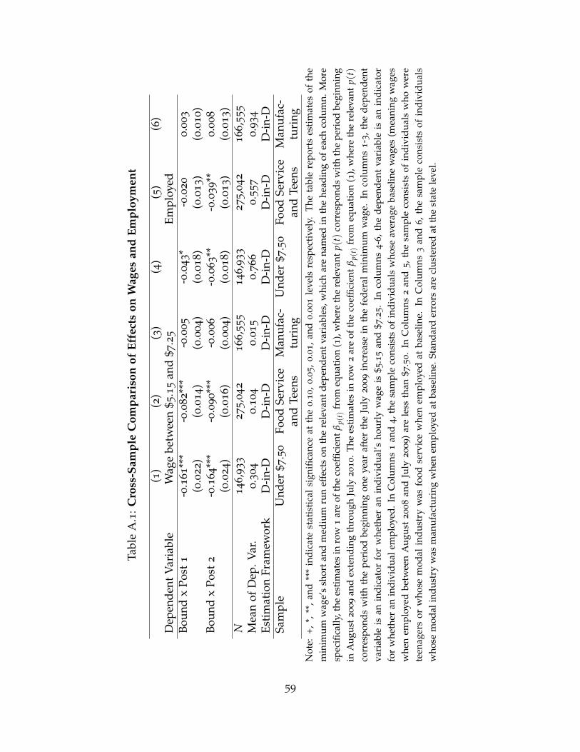
Tabl

eA

.1:C

ross

-Sam

ple

Com

pari

son

ofEf

fect

son

Wag

esan

dEm

ploy

men

t

(1)

(2)

(3)

(4)

(5)

(6)

Dep

ende

ntV

aria

ble

Wag

ebe

twee

n$5

.15

and

$7.2

5Em

ploy

edBo

und

xPo

st1

-0.1

61**

*-0

.082**

*-0

.005

-0.0

43*

-0.0

20

0.0

03

(0.0

22)

(0.0

14)

(0.0

04)

(0.0

18)

(0.0

13)

(0.0

10)

Boun

dx

Post

2-0

.164**

*-0

.090**

*-0

.006

-0.0

63**

-0.0

39**

0.0

08

(0.0

24)

(0.0

16)

(0.0

04)

(0.0

18)

(0.0

13)

(0.0

13)

N146,9

33

275

,042

166,5

55

146,9

33

275,0

42

166,5

55

Mea

nof

Dep

.Var

.0.3

04

0.1

04

0.0

15

0.7

66

0.5

57

0.9

34

Esti

mat

ion

Fram

ewor

kD

-in-

DD

-in-

DD

-in-

DD

-in-

DD

-in-

DD

-in-

DSa

mpl

eU

nder

$7.5

0Fo

odSe

rvic

eM

anuf

ac-

Und

er$7

.50

Food

Serv

ice

Man

ufac

-an

dTe

ens

turi

ngan

dTe

ens

turi

ngN

ote:

+,*,

**,

and

***

indi

cate

stat

isti

cal

sign

ifica

nce

atth

e0.1

0,

0.0

5,

0.0

1,

and

0.0

01

leve

lsre

spec

tive

ly.

The

tabl

ere

port

ses

tim

ates

ofth

em

inim

umw

age’

ssh

ort

and

med

ium

run

effe

cts

onth

ere

leva

ntde

pend

ent

vari

able

s,w

hich

are

nam

edin

the

head

ing

ofea

chco

lum

n.M

ore

spec

ifica

lly,t

hees

tim

ates

inro

w1

are

ofth

eco

effic

ient

βp(

t)fr

omeq

uati

on(1

),w

here

the

rele

vant

p(t)

corr

espo

nds

wit

hth

epe

riod

begi

nnin

gin

Aug

ust2

009

and

exte

ndin

gth

roug

hJu

ly2010.T

hees

tim

ates

inro

w2

are

ofth

eco

effic

ient

βp(

t)fr

omeq

uati

on(1

),w

here

the

rele

vant

p(t)

corr

espo

nds

wit

hth

epe

riod

begi

nnin

gon

eye

araf

ter

the

July

2009

incr

ease

inth

efe

dera

lm

inim

umw

age.

Inco

lum

ns1-3

,the

depe

nden

tva

riab

leis

anin

dica

tor

for

whe

ther

anin

divi

dual

’sho

urly

wag

eis

$5.1

5an

d$7

.25.

Inco

lum

ns4-6

,the

depe

nden

tva

riab

leis

anin

dica

tor

for

whe

ther

anin

divi

dual

empl

oyed

.In

Col

umns

1an

d4,t

hesa

mpl

eco

nsis

tsof

indi

vidu

als

who

seav

erag

eba

selin

ew

ages

(mea

ning

wag

esw

hen

empl

oyed

betw

een

Aug

ust

2008

and

July

2009)

are

less

than

$7.5

0.

InC

olum

ns2

and

5,t

hesa

mpl

eco

nsis

tsof

indi

vidu

als

who

wer

ete

enag

ers

orw

hose

mod

alin

dust

ryw

asfo

odse

rvic

ew

hen

empl

oyed

atba

selin

e.In

Col

umns

3an

d6,

the

sam

ple

cons

ists

ofin

divi

dual

sw

hose

mod

alin

dust

ryw

asm

anuf

actu

ring

whe

nem

ploy

edat

base

line.

Stan

dard

erro

rsar

ecl

uste

red

atth

est

ate

leve

l.

59

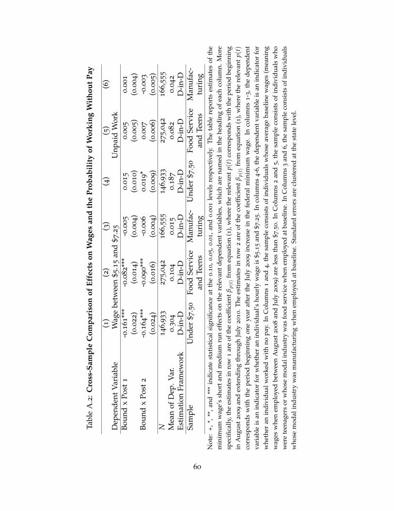
Tabl

eA

.2:C

ross

-Sam

ple

Com

pari

son

ofEf

fect

son

Wag

esan

dth

ePr

obab

ilit

yof

Wor

king

Wit

hout

Pay

(1)

(2)

(3)

(4)

(5)

(6)

Dep

ende

ntV

aria

ble

Wag

ebe

twee

n$5

.15

and

$7.2

5U

npai

dW

ork

Boun

dx

Post

1-0

.161**

*-0

.082**

*-0

.005

0.0

15

0.0

05

0.0

01

(0.0

22)

(0.0

14)

(0.0

04)

(0.0

10)

(0.0

05)

(0.0

04)

Boun

dx

Post

2-0

.164**

*-0

.090**

*-0

.006

0.0

19*

0.0

07

-0.0

03

(0.0

24)

(0.0

16)

(0.0

04)

(0.0

09)

(0.0

06)

(0.0

05)

N146,9

33

275

,042

166,5

55

146,9

33

275,0

42

166,5

55

Mea

nof

Dep

.Var

.0.3

04

0.1

04

0.0

15

0.1

87

0.0

82

0.0

42

Esti

mat

ion

Fram

ewor

kD

-in-

DD

-in-

DD

-in-

DD

-in-

DD

-in-

DD

-in-

DSa

mpl

eU

nder

$7.5

0Fo

odSe

rvic

eM

anuf

ac-

Und

er$7

.50

Food

Serv

ice

Man

ufac

-an

dTe

ens

turi

ngan

dTe

ens

turi

ngN

ote:

+,*,

**,

and

***

indi

cate

stat

isti

cal

sign

ifica

nce

atth

e0.1

0,

0.0

5,

0.0

1,

and

0.0

01

leve

lsre

spec

tive

ly.

The

tabl

ere

port

ses

tim

ates

ofth

em

inim

umw

age’

ssh

ort

and

med

ium

run

effe

cts

onth

ere

leva

ntde

pend

ent

vari

able

s,w

hich

are

nam

edin

the

head

ing

ofea

chco

lum

n.M

ore

spec

ifica

lly,t

hees

tim

ates

inro

w1

are

ofth

eco

effic

ient

βp(

t)fr

omeq

uati

on(1

),w

here

the

rele

vant

p(t)

corr

espo

nds

wit

hth

epe

riod

begi

nnin

gin

Aug

ust2

009

and

exte

ndin

gth

roug

hJu

ly2010.T

hees

tim

ates

inro

w2

are

ofth

eco

effic

ient

βp(

t)fr

omeq

uati

on(1

),w

here

the

rele

vant

p(t)

corr

espo

nds

wit

hth

epe

riod

begi

nnin

gon

eye

araf

ter

the

July

2009

incr

ease

inth

efe

dera

lm

inim

umw

age.

Inco

lum

ns1-3

,the

depe

nden

tva

riab

leis

anin

dica

tor

for

whe

ther

anin

divi

dual

’sho

urly

wag

eis

$5.1

5an

d$7

.25.I

nco

lum

ns4-6

,the

depe

nden

tvar

iabl

eis

anin

dica

tor

for

whe

ther

anin

divi

dual

wor

ked

wit

hno

pay.

InC

olum

ns1

and

4,t

hesa

mpl

eco

nsis

tsof

indi

vidu

als

who

seav

erag

eba

selin

ew

ages

(mea

ning

wag

esw

hen

empl

oyed

betw

een

Aug

ust

2008

and

July

2009)

are

less

than

$7.5

0.

InC

olum

ns2

and

5,t

hesa

mpl

eco

nsis

tsof

indi

vidu

als

who

wer

ete

enag

ers

orw

hose

mod

alin

dust

ryw

asfo

odse

rvic

ew

hen

empl

oyed

atba

selin

e.In

Col

umns

3an

d6,t

hesa

mpl

eco

nsis

tsof

indi

vidu

als

who

sem

odal

indu

stry

was

man

ufac

turi

ngw

hen

empl

oyed

atba

selin

e.St

anda

rder

rors

are

clus

tere

dat

the

stat

ele

vel.

60

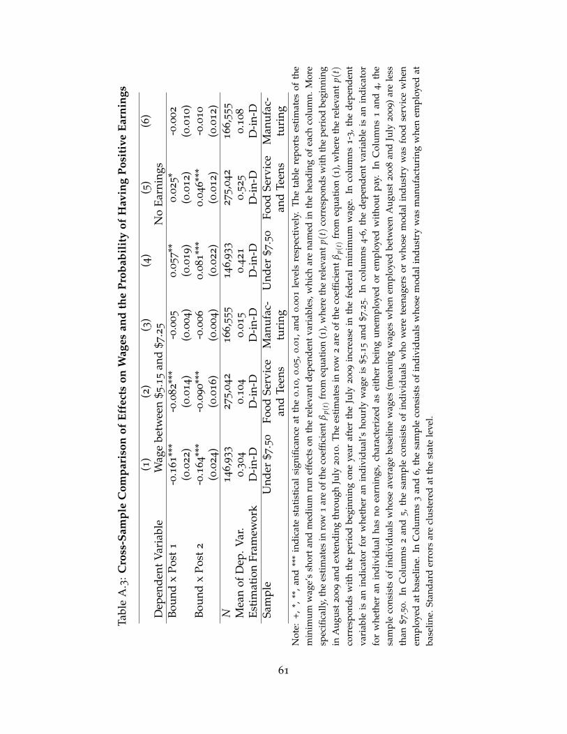
Tabl

eA

.3:C

ross

-Sam

ple

Com

pari

son

ofEf

fect

son

Wag

esan

dth

ePr

obab

ilit

yof

Hav

ing

Posi

tive

Earn

ings

(1)

(2)

(3)

(4)

(5)

(6)

Dep

ende

ntV

aria

ble

Wag

ebe

twee

n$5

.15

and

$7.2

5N

oEa

rnin

gsBo

und

xPo

st1

-0.1

61**

*-0

.082**

*-0

.005

0.0

57**

0.0

25*

-0.0

02

(0.0

22)

(0.0

14)

(0.0

04)

(0.0

19)

(0.0

12)

(0.0

10)

Boun

dx

Post

2-0

.164**

*-0

.090**

*-0

.006

0.0

81**

*0.0

46**

*-0

.010

(0.0

24)

(0.0

16)

(0.0

04)

(0.0

22)

(0.0

12)

(0.0

12)

N146,9

33

275

,042

166,5

55

146,9

33

275,0

42

166,5

55

Mea

nof

Dep

.Var

.0.3

04

0.1

04

0.0

15

0.4

21

0.5

25

0.1

08

Esti

mat

ion

Fram

ewor

kD

-in-

DD

-in-

DD

-in-

DD

-in-

DD

-in-

DD

-in-

DSa

mpl

eU

nder

$7.5

0Fo

odSe

rvic

eM

anuf

ac-

Und

er$7

.50

Food

Serv

ice

Man

ufac

-an

dTe

ens

turi

ngan

dTe

ens

turi

ngN

ote:

+,*,

**,

and

***

indi

cate

stat

isti

cal

sign

ifica

nce

atth

e0.1

0,

0.0

5,

0.0

1,

and

0.0

01

leve

lsre

spec

tive

ly.

The

tabl

ere

port

ses

tim

ates

ofth

em

inim

umw

age’

ssh

ort

and

med

ium

run

effe

cts

onth

ere

leva

ntde

pend

ent

vari

able

s,w

hich

are

nam

edin

the

head

ing

ofea

chco

lum

n.M

ore

spec

ifica

lly,t

hees

tim

ates

inro

w1

are

ofth

eco

effic

ient

βp(

t)fr

omeq

uati

on(1

),w

here

the

rele

vant

p(t)

corr

espo

nds

wit

hth

epe

riod

begi

nnin

gin

Aug

ust2

009

and

exte

ndin

gth

roug

hJu

ly2010.T

hees

tim

ates

inro

w2

are

ofth

eco

effic

ient

βp(

t)fr

omeq

uati

on(1

),w

here

the

rele

vant

p(t)

corr

espo

nds

wit

hth

epe

riod

begi

nnin

gon

eye

araf

ter

the

July

2009

incr

ease

inth

efe

dera

lm

inim

umw

age.

Inco

lum

ns1-3

,the

depe

nden

tva

riab

leis

anin

dica

tor

for

whe

ther

anin

divi

dual

’sho

urly

wag

eis

$5.1

5an

d$7

.25.

Inco

lum

ns4-6

,the

depe

nden

tva

riab

leis

anin

dica

tor

for

whe

ther

anin

divi

dual

has

noea

rnin

gs,

char

acte

rize

das

eith

erbe

ing

unem

ploy

edor

empl

oyed

wit

hout

pay.

InC

olum

ns1

and

4,

the

sam

ple

cons

ists

ofin

divi

dual

sw

hose

aver

age

base

line

wag

es(m

eani

ngw

ages

whe

nem

ploy

edbe

twee

nA

ugus

t2008

and

July

2009)

are

less

than

$7.5

0.

InC

olum

ns2

and

5,

the

sam

ple

cons

ists

ofin

divi

dual

sw

how

ere

teen

ager

sor

who

sem

odal

indu

stry

was

food

serv

ice

whe

nem

ploy

edat

base

line.

InC

olum

ns3

and

6,t

hesa

mpl

eco

nsis

tsof

indi

vidu

als

who

sem

odal

indu

stry

was

man

ufac

turi

ngw

hen

empl

oyed

atba

selin

e.St

anda

rder

rors

are

clus

tere

dat

the

stat

ele

vel.

61

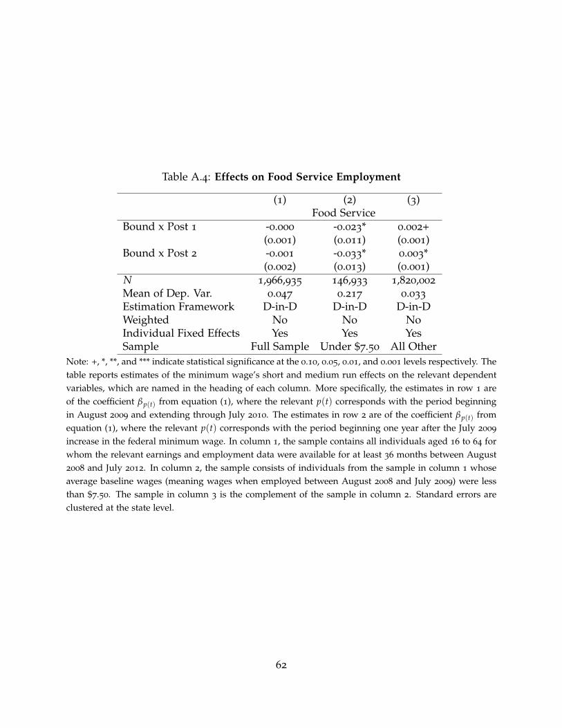
Table A.4: Effects on Food Service Employment

(1) (2) (3)Food Service

Bound x Post 1 -0.000 -0.023* 0.002+(0.001) (0.011) (0.001)

Bound x Post 2 -0.001 -0.033* 0.003*(0.002) (0.013) (0.001)

N 1,966,935 146,933 1,820,002

Mean of Dep. Var. 0.047 0.217 0.033

Estimation Framework D-in-D D-in-D D-in-DWeighted No No NoIndividual Fixed Effects Yes Yes YesSample Full Sample Under $7.50 All Other

Note: +, *, **, and *** indicate statistical significance at the 0.10, 0.05, 0.01, and 0.001 levels respectively. Thetable reports estimates of the minimum wage’s short and medium run effects on the relevant dependentvariables, which are named in the heading of each column. More specifically, the estimates in row 1 areof the coefficient βp(t) from equation (1), where the relevant p(t) corresponds with the period beginningin August 2009 and extending through July 2010. The estimates in row 2 are of the coefficient βp(t) fromequation (1), where the relevant p(t) corresponds with the period beginning one year after the July 2009

increase in the federal minimum wage. In column 1, the sample contains all individuals aged 16 to 64 forwhom the relevant earnings and employment data were available for at least 36 months between August2008 and July 2012. In column 2, the sample consists of individuals from the sample in column 1 whoseaverage baseline wages (meaning wages when employed between August 2008 and July 2009) were lessthan $7.50. The sample in column 3 is the complement of the sample in column 2. Standard errors areclustered at the state level.

62

Tabl

eA

.5:F

irst

Stag

ean

dEm

ploy

men

tEf

fect

sfo

rA

llA

dult

s

(1)

(2)

(3)

(4)

(5)

Pane

lA:

Dep

ende

ntV

aria

ble:

Aff

ecte

dW

age

Boun

dx

Post

10.0

01

-0.1

61**

*-0

.036**

*-0

.008*

-0.0

00

(0.0

01)

(0.0

22)

(0.0

10)

(0.0

04)

(0.0

01)

Boun

dx

Post

20.0

01

-0.1

64**

*-0

.042**

*-0

.007

-0.0

00

(0.0

01)

(0.0

24)

(0.0

08)

(0.0

05)

(0.0

01)

N520,0

74

146,9

33

102,1

54

122,5

94

1,0

75,1

80

Mea

nof

Dep

.Var

.0.0

00

0.3

04

0.0

57

0.0

27

0.0

04

Esti

mat

ion

Fram

ewor

kD

-in-

DD

-in-

DD

-in-

DD

-in-

DD

-in-

D

Pane

lB:

Dep

ende

ntV

aria

ble:

Empl

oym

ent

Boun

dx

Post

1-0

.004

-0.0

43*

0.0

20

-0.0

11

0.0

05

(0.0

04)

(0.0

18)

(0.0

22)

(0.0

11)

(0.0

05)

Boun

dx

Post

2-0

.013

-0.0

63**

-0.0

11

-0.0

08

0.0

00

(0.0

09)

(0.0

18)

(0.0

23)

(0.0

13)

(0.0

07)

N520,0

74

146,9

33

102,1

54

122,5

94

1,0

75,1

80

Mea

nof

Dep

.Var

.0.0

00

0.7

66

0.8

13

0.8

77

0.9

46

Esti

mat

ion

Fram

ewor

kD

-in-

DD

-in-

DD

-in-

DD

-in-

DD

-in-

DSa

mpl

eU

nem

p.at

Base

Und

er$7

.50

$7.5

0-$

8.4

9$8

.50-$

9.9

9O

ver

$10.0

0

Not

e:+,

*,**

,and

***

indi

cate

stat

isti

cals

igni

fican

ceat

the

0.1

0,0

.05,0

.01,a

nd0.0

01

leve

lsre

spec

tive

ly.

Inpa

nelA

the

depe

nden

tva

riab

lein

this

pane

lis

anin

dica

tor

equa

lto

1if

anin

divi

dual

repo

rts

aw

age

betw

een

$5.1

5an

d$7

.25

inth

ere

leva

ntm

onth

.In

pane

lBth

ede

pend

ent

vari

able

isan

indi

cato

req

ualt

o1

ifan

indi

vidu

alis

empl

oyed

.In

both

pane

ls,t

hees

tim

ates

inro

w1

are

ofth

eco

effic

ient

βp(

t)fr

omeq

uati

on(1

),w

here

the

rele

vant

p(t)

corr

espo

nds

wit

hth

epe

riod

begi

nnin

gin

July

2009

and

exte

ndin

gth

roug

hJu

ly2010.

The

sam

ples

used

acro

ssco

lum

ns1

thro

ugh

5fu

llypa

rtit

ion

the

set

ofal

lin

divi

dual

sag

ed16

to64

for

who

mth

ere

leva

ntea

rnin

gsan

dem

ploy

men

tda

taw

ere

avai

labl

efo

rat

leas

t36

mon

ths

betw

een

Aug

ust

2008

and

July

2012.

The

esti

mat

esin

row

2ar

eof

the

coef

ficie

ntβ

p(t)

from

equa

tion

(1),

whe

reth

ere

leva

ntp(

t)co

rres

pond

sw

ith

the

peri

odbe

ginn

ing

one

year

afte

rth

eJu

ly2009

incr

ease

inth

efe

dera

lmin

imum

wag

e.St

anda

rder

rors

are

clus

tere

dat

the

stat

ele

vel.

63

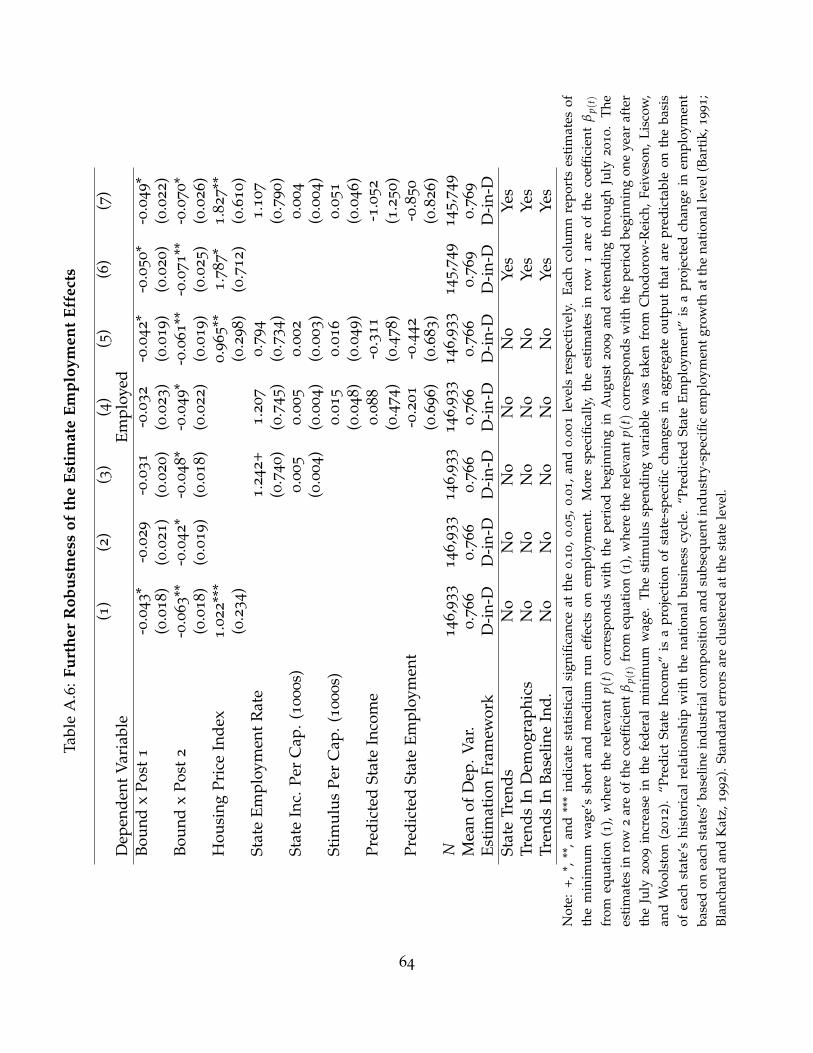
Tabl

eA

.6:F

urth

erR

obus

tnes

sof

the

Esti

mat

eEm

ploy

men

tEf

fect

s

(1)

(2)

(3)

(4)

(5)

(6)

(7)

Dep

ende

ntV

aria

ble

Empl

oyed

Boun

dx

Post

1-0

.043*

-0.0

29

-0.0

31

-0.0

32

-0.0

42*

-0.0

50*

-0.0

49*

(0.0

18)

(0.0

21)

(0.0

20)

(0.0

23)

(0.0

19)

(0.0

20)

(0.0

22)

Boun

dx

Post

2-0

.063**

-0.0

42*

-0.0

48*

-0.0

49*

-0.0

61**

-0.0

71**

-0.0

70*

(0.0

18)

(0.0

19)

(0.0

18)

(0.0

22)

(0.0

19)

(0.0

25)

(0.0

26)

Hou

sing

Pric

eIn

dex

1.0

22**

*0.9

65**

1.7

87*

1.8

27**

(0.2

34)

(0.2

98)

(0.7

12)

(0.6

10)

Stat

eEm

ploy

men

tR

ate

1.2

42+

1.2

07

0.7

94

1.1

07

(0.7

40)

(0.7

45)

(0.7

34)

(0.7

90)

Stat

eIn

c.Pe

rC

ap.(

1000s)

0.0

05

0.0

05

0.0

02

0.0

04

(0.0

04)

(0.0

04)

(0.0

03)

(0.0

04)

Stim

ulus

Per

Cap

.(1000s)

0.0

15

0.0

16

0.0

51

(0.0

48)

(0.0

49)

(0.0

46)

Pred

icte

dSt

ate

Inco

me

0.0

88

-0.3

11

-1.0

52

(0.4

74)

(0.4

78)

(1.2

50)

Pred

icte

dSt

ate

Empl

oym

ent

-0.2

01

-0.4

42

-0.8

50

(0.6

96)

(0.6

83)

(0.8

26)

N146,9

33

146,9

33

146,9

33

146,9

33

146,9

33

145,7

49

145,7

49

Mea

nof

Dep

.Var

.0.7

66

0.7

66

0.7

66

0.7

66

0.7

66

0.7

69

0.7

69

Esti

mat

ion

Fram

ewor

kD

-in-

DD

-in-

DD

-in-

DD

-in-

DD

-in-

DD

-in-

DD

-in-

DSt

ate

Tren

dsN

oN

oN

oN

oN

oYe

sYe

sTr

ends

InD

emog

raph

ics

No

No

No

No

No

Yes

Yes

Tren

dsIn

Base

line

Ind.

No

No

No

No

No

Yes

Yes

Not

e:+,

*,**

,an

d**

*in

dica

test

atis

tica

lsi

gnifi

canc

eat

the

0.1

0,

0.0

5,

0.0

1,

and

0.0

01

leve

lsre

spec

tive

ly.

Each

colu

mn

repo

rts

esti

mat

esof

the

min

imum

wag

e’s

shor

tan

dm

ediu

mru

nef

fect

son

empl

oym

ent.

Mor

esp

ecifi

cally

,th

ees

tim

ates

inro

w1

are

ofth

eco

effic

ient

βp(

t)

from

equa

tion

(1),

whe

reth

ere

leva

ntp(

t)co

rres

pond

sw

ith

the

peri

odbe

ginn

ing

inA

ugus

t2009

and

exte

ndin

gth

roug

hJu

ly2010.

The

esti

mat

esin

row

2ar

eof

the

coef

ficie

ntβ

p(t)

from

equa

tion

(1),

whe

reth

ere

leva

ntp(

t)co

rres

pond

sw

ith

the

peri

odbe

ginn

ing

one

year

afte

rth

eJu

ly2009

incr

ease

inth

efe

dera

lm

inim

umw

age.

The

stim

ulus

spen

ding

vari

able

was

take

nfr

omC

hodo

row

-Rei

ch,

Feiv

eson

,Li

scow

,an

dW

ools

ton

(2012).

“Pre

dict

Stat

eIn

com

e”is

apr

ojec

tion

ofst

ate-

spec

ific

chan

ges

inag

greg

ate

outp

utth

atar

epr

edic

tabl

eon

the

basi

sof

each

stat

e’s

hist

oric

alre

lati

onsh

ipw

ith

the

nati

onal

busi

ness

cycl

e.“P

redi

cted

Stat

eEm

ploy

men

t”is

apr

ojec

ted

chan

gein

empl

oym

ent

base

don

each

stat

es’b

asel

ine

indu

stri

alco

mpo

siti

onan

dsu

bseq

uent

indu

stry

-spe

cific

empl

oym

entg

row

that

the

nati

onal

leve

l(Ba

rtik

,1991;

Blan

char

dan

dK

atz,

1992).

Stan

dard

erro

rsar

ecl

uste

red

atth

est

ate

leve

l.

64

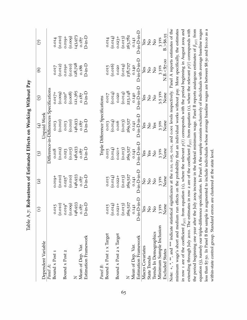
Tabl

eA

.7:R

obus

tnes

sof

Esti

mat

edEf

fect

son

Wor

king

Wit

hout

Pay

(1)

(2)

(3)

(4)

(5)

(6)

(7)

Dep

ende

ntV

aria

ble

Unp

aid

Wor

kPa

nelA

:D

iffer

ence

-in-

Diff

eren

ces

Spec

ifica

tion

sBo

und

xPo

st1

0.0

15

0.0

19+

0.0

18

0.0

13

0.0

17+

0.0

17

0.0

14

(0.0

10)

(0.0

10)

(0.0

12)

(0.0

10)

(0.0

09)

(0.0

12)

(0.0

10)

Boun

dx

Post

20.0

19*

0.0

25*

0.0

23

0.0

13

0.0

20*

0.0

19+

0.0

19+

(0.0

09)

(0.0

10)

(0.0

15)

(0.0

10)

(0.0

08)

(0.0

10)

(0.0

09)

N146,9

33

146,9

33

146,9

33

146,9

33

121,3

65

128,7

28

143,9

73

Mea

nof

Dep

.Var

.0.1

87

0.1

87

0.1

87

0.1

87

0.1

87

0.1

86

0.1

87

Esti

mat

ion

Fram

ewor

kD

-in-

DD

-in-

DD

-in-

DD

-in-

DD

-in-

DD

-in-

DD

-in-

D

Pane

lB:

Trip

leD

iffer

ence

Spec

ifica

tion

sBo

und

xPo

st1

xTa

rget

0.0

15

0.0

15

0.0

15

0.0

13

0.0

17

0.0

15

0.0

14

(0.0

14)

(0.0

14)

(0.0

14)

(0.0

14)

(0.0

14)

(0.0

16)

(0.0

14)

Boun

dx

Post

2x

Targ

et0.0

21+

0.0

22+

0.0

21+

0.0

16

0.0

20

0.0

20

0.0

23+

(0.0

13)

(0.0

13)

(0.0

13)

(0.0

13)

(0.0

14)

(0.0

14)

(0.0

13)

N269,5

27

269,5

27

269,5

27

269,5

27

223,1

48

238,7

27

263,7

82

Mea

nof

Dep

.Var

.0.1

41

0.1

41

0.1

41

0.1

41

0.1

40

0.1

40

0.1

41

Esti

mat

ion

Fram

ewor

kD

-in-

D-i

n-D

D-i

n-D

-in-

DD

-in-

D-i

n-D

D-i

n-D

-in-

DD

-in-

D-i

n-D

D-i

n-D

-in-

DD

-in-

D-i

n-D

Mac

roC

ovar

iate

sYe

sN

oYe

sYe

sYe

sYe

sYe

sSt

ate

Tren

dsN

oN

oYe

sN

oN

oN

oN

oTr

ends

InD

emog

raph

ics

No

No

No

Yes

No

No

No

Min

imum

Sam

ple

Incl

usio

n3

yrs

3yr

s3

yrs

3yr

s3.5

yrs

3yr

s3

yrs

Excl

uded

Stat

esN

one

Non

eN

one

Non

eN

one

N.B

.<$7

.00

B.>

$6.5

5

Not

e:+,

*,**

,an

d**

*in

dica

test

atis

tica

lsi

gnifi

canc

eat

the

0.1

0,

0.0

5,

0.0

1,

and

0.0

01

leve

lsre

spec

tive

ly.

Pane

lA

repo

rts

esti

mat

esof

the

min

imum

wag

e’s

shor

tan

dm

ediu

mru

nef

fect

son

the

prob

abili

tyth

atan

indi

vidu

alw

orks

wit

hout

pay.

Mor

esp

ecifi

cally

,th

ees

tim

ates

inro

w1

are

ofth

eco

effic

ient

βp(

t)fr

omeq

uati

on(1

),w

here

the

rele

vant

p(t)

corr

espo

nds

wit

hth

epe

riod

begi

nnin

gin

Aug

ust

2009

and

exte

ndin

gth

roug

hJu

ly2010.

The

esti

mat

esin

row

2ar

eof

the

coef

ficie

ntβ

p(t)

from

equa

tion

(1),

whe

reth

ere

leva

ntp(

t)co

rres

pond

sw

ith

the

peri

odbe

ginn

ing

one

year

afte

rth

eJu

ly2009

incr

ease

inth

efe

dera

lm

inim

umw

age.

Pane

lB

repo

rts

anal

ogou

ses

tim

ates

ofβ

p(t)

from

equa

tion

(3),

nam

ely

our

trip

le-d

iffer

ence

spec

ifica

tion

.In

Pane

lAth

esa

mpl

eco

nsis

tsex

clus

ivel

yof

indi

vidu

als

wit

hav

erag

eba

selin

ew

ages

less

than

$7.5

0.

InPa

nelB

the

sam

ple

isau

gmen

ted

toin

clud

ein

divi

dual

sw

hose

aver

age

base

line

wag

esar

ebe

twee

n$8

.50

and

$10.0

0as

aw

ithi

n-st

ate

cont

rolg

roup

.Sta

ndar

der

rors

are

clus

tere

dat

the

stat

ele

vel.

65

Tabl

eA

.8:R

obus

tnes

sof

Esti

mat

edEf

fect

son

Hav

ing

No

Earn

ings

(1)

(2)

(3)

(4)

(5)

(6)

(7)

Dep

ende

ntV

aria

ble

No

Earn

ings

Pane

lA:

Diff

eren

ce-i

n-D

iffer

ence

sSp

ecifi

cati

ons

Boun

dx

Post

10.0

57**

0.0

47*

0.0

69**

*0.0

54**

0.0

59**

0.0

66**

0.0

55**

(0.0

19)

(0.0

21)

(0.0

19)

(0.0

19)

(0.0

20)

(0.0

19)

(0.0

19)

Boun

dx

Post

20.0

81**

*0.0

67**

0.0

94**

*0.0

74**

0.0

81**

*0.0

86**

0.0

77**

*(0

.022)

(0.0

21)

(0.0

25)

(0.0

21)

(0.0

18)

(0.0

26)

(0.0

22)

N146,9

33

146,9

33

146,9

33

146,9

33

121,3

65

128,7

28

143,9

73

Mea

nof

Dep

.Var

.0.4

21

0.4

21

0.4

21

0.4

21

0.4

18

0.4

21

0.4

22

Esti

mat

ion

Fram

ewor

kD

-in-

DD

-in-

DD

-in-

DD

-in-

DD

-in-

DD

-in-

DD

-in-

D

Pane

lB:

Trip

leD

iffer

ence

Spec

ifica

tion

sBo

und

xPo

st1

xTa

rget

0.0

47*

0.0

33

0.0

46+

0.0

46+

0.0

44+

0.0

55*

0.0

48*

(0.0

23)

(0.0

26)

(0.0

23)

(0.0

24)

(0.0

24)

(0.0

24)

(0.0

23)

Boun

dx

Post

2x

Targ

et0.0

80**

0.0

60*

0.0

80**

0.0

80**

0.0

72**

0.0

80**

0.0

76**

(0.0

23)

(0.0

25)

(0.0

23)

(0.0

25)

(0.0

23)

(0.0

25)

(0.0

23)

N269,5

27

269,5

27

269,5

27

269,5

27

223,1

48

238,7

27

263,7

82

Mea

nof

Dep

.Var

.0.3

24

0.3

24

0.3

24

0.3

24

0.3

20

0.3

23

0.3

26

Esti

mat

ion

Fram

ewor

kD

-in-

D-i

n-D

D-i

n-D

-in-

DD

-in-

D-i

n-D

D-i

n-D

-in-

DD

-in-

D-i

n-D

D-i

n-D

-in-

DD

-in-

D-i

n-D

Mac

roC

ovar

iate

sYe

sN

oYe

sYe

sYe

sYe

sYe

sSt

ate

Tren

dsN

oN

oYe

sN

oN

oN

oN

oTr

ends

InD

emog

raph

ics

No

No

No

Yes

No

No

No

Min

imum

Sam

ple

Incl

usio

n3

yrs

3yr

s3

yrs

3yr

s3.5

yrs

3yr

s3

yrs

Excl

uded

Stat

esN

one

Non

eN

one

Non

eN

one

N.B

.<$7

.00

B.>

$6.5

5

Not

e:+,

*,**

,an

d**

*in

dica

test

atis

tica

lsi

gnifi

canc

eat

the

0.1

0,

0.0

5,

0.0

1,

and

0.0

01

leve

lsre

spec

tive

ly.

Pane

lA

repo

rts

esti

mat

esof

the

min

imum

wag

e’s

shor

tand

med

ium

run

effe

cts

onth

epr

obab

ility

that

anin

divi

dual

has

noea

rnin

gs.M

ore

spec

ifica

lly,t

hees

tim

ates

inro

w1

are

ofth

eco

effic

ient

βp(

t)fr

omeq

uati

on(1

),w

here

the

rele

vant

p(t)

corr

espo

nds

wit

hth

epe

riod

begi

nnin

gin

Aug

ust

2009

and

exte

ndin

gth

roug

hJu

ly2010.

The

esti

mat

esin

row

2ar

eof

the

coef

ficie

ntβ

p(t)

from

equa

tion

(1),

whe

reth

ere

leva

ntp(

t)co

rres

pond

sw

ith

the

peri

odbe

ginn

ing

one

year

afte

rth

eJu

ly2009

incr

ease

inth

efe

dera

lmin

imum

wag

e.Pa

nelB

repo

rts

anal

ogou

ses

tim

ates

ofβ

p(t)

from

equa

tion

(3),

nam

ely

our

trip

le-d

iffer

ence

spec

ifica

tion

.In

Pane

lA

the

sam

ple

cons

ists

excl

usiv

ely

ofin

divi

dual

sw

ith

aver

age

base

line

wag

esle

ssth

an$7

.50.I

nPa

nelB

the

sam

ple

isau

gmen

ted

toin

clud

ein

divi

dual

sw

hose

aver

age

base

line

wag

esar

ebe

twee

n$8

.50

and

$10.0

0as

aw

ithi

n-st

ate

cont

rolg

roup

.Sta

ndar

der

rors

are

clus

tere

dat

the

stat

ele

vel.

66

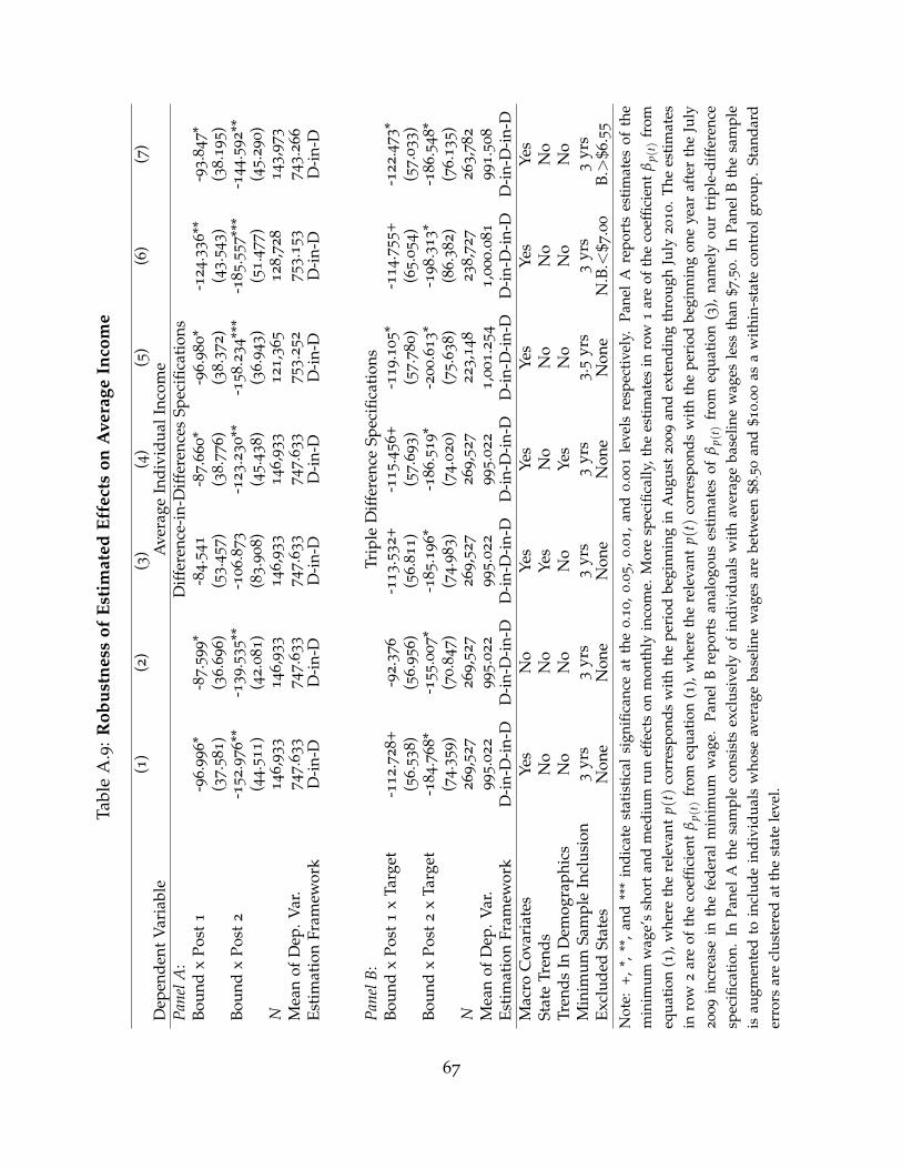
Tabl

eA

.9:R

obus

tnes

sof

Esti

mat

edEf

fect

son

Ave

rage

Inco

me

(1)

(2)

(3)

(4)

(5)

(6)

(7)

Dep

ende

ntV

aria

ble

Ave

rage

Indi

vidu

alIn

com

ePa

nelA

:D

iffer

ence

-in-

Diff

eren

ces

Spec

ifica

tion

sBo

und

xPo

st1

-96.9

96*

-87.5

99*

-84.5

41

-87.6

60*

-96.9

80*

-124.3

36**

-93.8

47*

(37.5

81)

(36.6

96)

(53.4

57)

(38.7

76)

(38.3

72)

(43.5

43)

(38.1

95)

Boun

dx

Post

2-1

52.9

76**

-139.5

35**

-106.8

73

-123.2

30**

-158.2

34**

*-1

85.5

57**

*-1

44.5

92**

(44.5

11)

(42.0

81)

(83.9

08)

(45.4

38)

(36.9

43)

(51.4

77)

(45.2

90)

N146,9

33

146,9

33

146,9

33

146,9

33

121,3

65

128,7

28

143,9

73

Mea

nof

Dep

.Var

.747.6

33

747.6

33

747.6

33

747.6

33

753.2

52

753.1

53

743.2

66

Esti

mat

ion

Fram

ewor

kD

-in-

DD

-in-

DD

-in-

DD

-in-

DD

-in-

DD

-in-

DD

-in-

D

Pane

lB:

Trip

leD

iffer

ence

Spec

ifica

tion

sBo

und

xPo

st1

xTa

rget

-112.7

28+

-92.3

76

-113.5

32+

-115.4

56+

-119.1

05*

-114.7

55+

-122.4

73*

(56.5

38)

(56.9

56)

(56.8

11)

(57.6

93)

(57.7

80)

(65.0

54)

(57.0

33)

Boun

dx

Post

2x

Targ

et-1

84.7

68*

-155.0

07*

-185.1

96*

-186.5

19*

-200.6

13*

-198.3

13*

-186.5

48*

(74.3

59)

(70.8

47)

(74.9

83)

(74.0

20)

(75.6

38)

(86.3

82)

(76.1

35)

N269,5

27

269,5

27

269,5

27

269,5

27

223,1

48

238,7

27

263,7

82

Mea

nof

Dep

.Var

.995.0

22

995.0

22

995.0

22

995.0

22

1,0

01.2

54

1,0

00.0

81

991.5

08

Esti

mat

ion

Fram

ewor

kD

-in-

D-i

n-D

D-i

n-D

-in-

DD

-in-

D-i

n-D

D-i

n-D

-in-

DD

-in-

D-i

n-D

D-i

n-D

-in-

DD

-in-

D-i

n-D

Mac

roC

ovar

iate

sYe

sN

oYe

sYe

sYe

sYe

sYe

sSt

ate

Tren

dsN

oN

oYe

sN

oN

oN

oN

oTr

ends

InD

emog

raph

ics

No

No

No

Yes

No

No

No

Min

imum

Sam

ple

Incl

usio

n3

yrs

3yr

s3

yrs

3yr

s3.5

yrs

3yr

s3

yrs

Excl

uded

Stat

esN

one

Non

eN

one

Non

eN

one

N.B

.<$7

.00

B.>

$6.5

5

Not

e:+,

*,**

,an

d**

*in

dica

test

atis

tica

lsi

gnifi

canc

eat

the

0.1

0,

0.0

5,

0.0

1,

and

0.0

01

leve

lsre

spec

tive

ly.

Pane

lA

repo

rts

esti

mat

esof

the

min

imum

wag

e’s

shor

tan

dm

ediu

mru

nef

fect

son

mon

thly

inco

me.

Mor

esp

ecifi

cally

,the

esti

mat

esin

row

1ar

eof

the

coef

ficie

ntβ

p(t)

from

equa

tion

(1),

whe

reth

ere

leva

ntp(

t)co

rres

pond

sw

ith

the

peri

odbe

ginn

ing

inA

ugus

t2009

and

exte

ndin

gth

roug

hJu

ly2010.

The

esti

mat

esin

row

2ar

eof

the

coef

ficie

ntβ

p(t)

from

equa

tion

(1),

whe

reth

ere

leva

ntp(

t)co

rres

pond

sw

ith

the

peri

odbe

ginn

ing

one

year

afte

rth

eJu

ly2009

incr

ease

inth

efe

dera

lm

inim

umw

age.

Pane

lB

repo

rts

anal

ogou

ses

tim

ates

ofβ

p(t)

from

equa

tion

(3),

nam

ely

our

trip

le-d

iffer

ence

spec

ifica

tion

.In

Pane

lA

the

sam

ple

cons

ists

excl

usiv

ely

ofin

divi

dual

sw

ith

aver

age

base

line

wag

esle

ssth

an$7

.50.

InPa

nel

Bth

esa

mpl

eis

augm

ente

dto

incl

ude

indi

vidu

als

who

seav

erag

eba

selin

ew

ages

are

betw

een

$8.5

0an

d$1

0.0

0as

aw

ithi

n-st

ate

cont

rol

grou

p.St

anda

rder

rors

are

clus

tere

dat

the

stat

ele

vel.

67

Tabl

eA

.10:R

obus

tnes

sof

Esti

mat

edEf

fect

son

Tran

siti

ons

into

Low

erM

iddl

eC

lass

Earn

ings

(1)

(2)

(3)

(4)

(5)

(6)

(7)

Dep

ende

ntV

aria

ble

Prob

abili

tyof

Earn

ing

$1500+

Pane

lA:

Diff

eren

ce-i

n-D

iffer

ence

sSp

ecifi

cati

ons

Boun

dx

Post

1-0

.016

-0.0

14

-0.0

07

-0.0

15

-0.0

11

-0.0

19

-0.0

17

(0.0

11)

(0.0

11)

(0.0

18)

(0.0

11)

(0.0

13)

(0.0

13)

(0.0

11)

Boun

dx

Post

2-0

.049**

*-0

.046**

-0.0

21

-0.0

43**

-0.0

53**

*-0

.056**

*-0

.048**

*(0

.013)

(0.0

13)

(0.0

25)

(0.0

13)

(0.0

14)

(0.0

14)

(0.0

13)

N146,9

33

146,9

33

146,9

33

146,9

33

121,3

65

128,7

28

143,9

73

Mea

nof

Dep

.Var

.0.2

06

0.2

06

0.2

06

0.2

06

0.2

03

0.2

20

0.2

06

Esti

mat

ion

Fram

ewor

kD

-in-

DD

-in-

DD

-in-

DD

-in-

DD

-in-

DD

-in-

DD

-in-

D

Pane

lB:

Trip

leD

iffer

ence

Spec

ifica

tion

sBo

und

xPo

st1

xTa

rget

-0.0

02

0.0

01

-0.0

02

-0.0

05

-0.0

17

0.0

02

-0.0

08

(0.0

18)

(0.0

16)

(0.0

18)

(0.0

18)

(0.0

22)

(0.0

20)

(0.0

18)

Boun

dx

Post

2x

Targ

et-0

.054*

-0.0

49*

-0.0

53*

-0.0

59*

-0.0

75**

-0.0

50+

-0.0

58*

(0.0

24)

(0.0

22)

(0.0

24)

(0.0

23)

(0.0

27)

(0.0

28)

(0.0

24)

N269,5

27

269,5

27

269,5

27

269,5

27

223,1

48

238,7

27

263,7

82

Mea

nof

Dep

.Var

.0.2

83

0.2

83

0.2

83

0.2

83

0.2

84

0.2

93

0.2

83

Esti

mat

ion

Fram

ewor

kD

-in-

D-i

n-D

D-i

n-D

-in-

DD

-in-

D-i

n-D

D-i

n-D

-in-

DD

-in-

D-i

n-D

D-i

n-D

-in-

DD

-in-

D-i

n-D

Mac

roC

ovar

iate

sYe

sN

oYe

sYe

sYe

sYe

sYe

sSt

ate

Tren

dsN

oN

oYe

sN

oN

oN

oN

oTr

ends

InD

emog

raph

ics

No

No

No

Yes

No

No

No

Min

imum

Sam

ple

Incl

usio

n3

yrs

3yr

s3

yrs

3yr

s3.5

yrs

3yr

s3

yrs

Excl

uded

Stat

esN

one

Non

eN

one

Non

eN

one

N.B

.<$7

.00

B.>

$6.5

5

Not

e:+,

*,**

,an

d**

*in

dica

test

atis

tica

lsi

gnifi

canc

eat

the

0.1

0,

0.0

5,

0.0

1,

and

0.0

01

leve

lsre

spec

tive

ly.

Pane

lA

repo

rts

esti

mat

esof

the

min

imum

wag

e’s

shor

tan

dm

ediu

mru

nef

fect

son

the

prob

abili

tyth

atan

indi

vidu

alha

sea

rnin

gsgr

eate

rth

an$1

500

ina

mon

th.

Mor

esp

ecifi

cally

,the

esti

mat

esin

row

1ar

eof

the

coef

ficie

ntβ

p(t)

from

equa

tion

(1),

whe

reth

ere

leva

ntp(

t)co

rres

pond

sw

ith

the

peri

odbe

ginn

ing

inA

ugus

t2009

and

exte

ndin

gth

roug

hJu

ly2010.

The

esti

mat

esin

row

2ar

eof

the

coef

ficie

ntβ

p(t)

from

equa

tion

(1),

whe

reth

ere

leva

ntp(

t)co

rres

pond

sw

ith

the

peri

odbe

ginn

ing

one

year

afte

rth

eJu

ly2009

incr

ease

inth

efe

dera

lm

inim

umw

age.

Pane

lB

repo

rts

anal

ogou

ses

tim

ates

ofβ

p(t)

from

equa

tion

(3),

nam

ely

our

trip

le-d

iffer

ence

spec

ifica

tion

.In

Pane

lAth

esa

mpl

eco

nsis

tsex

clus

ivel

yof

indi

vidu

als

wit

hav

erag

eba

selin

ew

ages

less

than

$7.5

0.I

nPa

nelB

the

sam

ple

isau

gmen

ted

toin

clud

ein

divi

dual

sw

hose

aver

age

base

line

wag

esar

ebe

twee

n$8

.50

and

$10.0

0as

aw

ithi

n-st

ate

cont

rolg

roup

.Sta

ndar

der

rors

are

clus

tere

dat

the

stat

ele

vel.

68

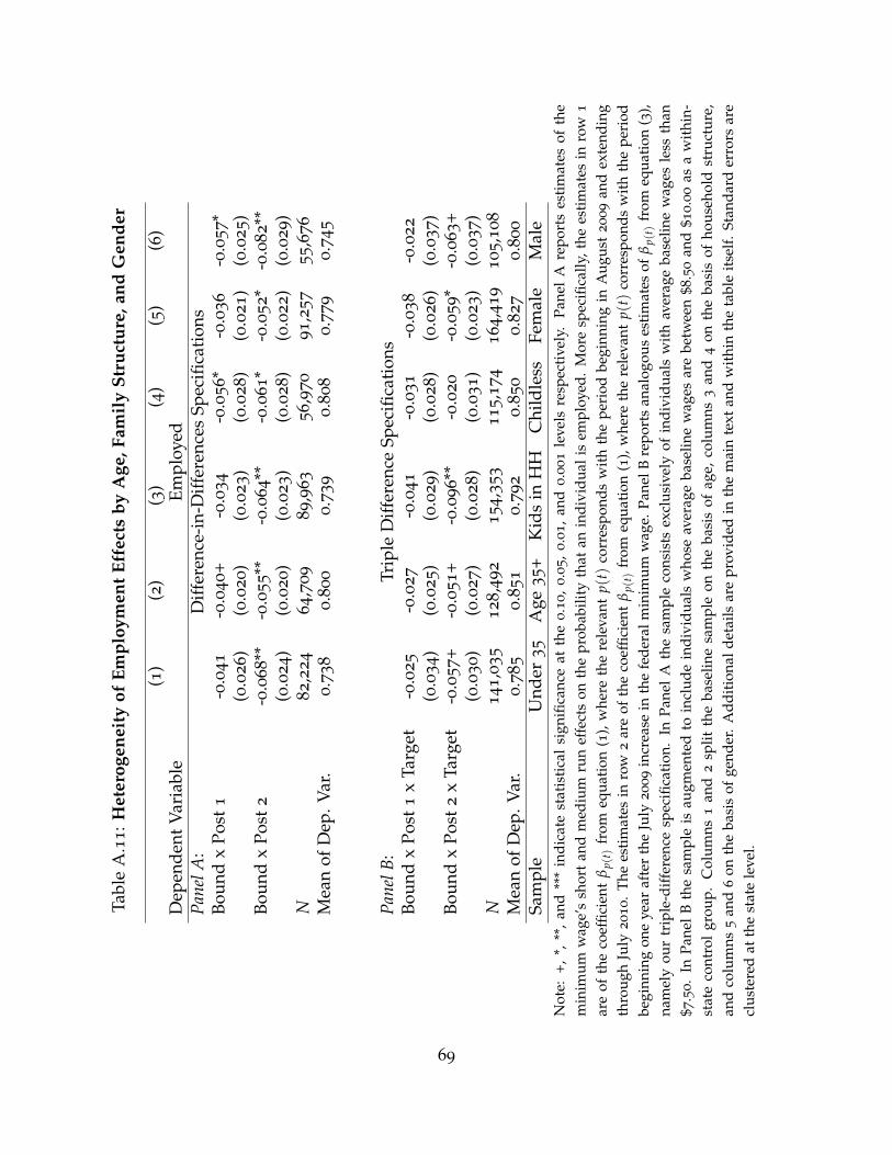
Tabl

eA

.11:H

eter

ogen

eity

ofEm

ploy

men

tEf

fect

sby

Age

,Fam

ily

Stru

ctur

e,an

dG

ende

r

(1)

(2)

(3)

(4)

(5)

(6)

Dep

ende

ntV

aria

ble

Empl

oyed

Pane

lA:

Diff

eren

ce-i

n-D

iffer

ence

sSp

ecifi

cati

ons

Boun

dx

Post

1-0

.041

-0.0

40+

-0.0

34

-0.0

56*

-0.0

36

-0.0

57*

(0.0

26)

(0.0

20)

(0.0

23)

(0.0

28)

(0.0

21)

(0.0

25)

Boun

dx

Post

2-0

.068**

-0.0

55**

-0.0

64**

-0.0

61*

-0.0

52*

-0.0

82**

(0.0

24)

(0.0

20)

(0.0

23)

(0.0

28)

(0.0

22)

(0.0

29)

N82,2

24

64,7

09

89,9

63

56,9

70

91,2

57

55,6

76

Mea

nof

Dep

.Var

.0.7

38

0.8

00

0.7

39

0.8

08

0.7

79

0.7

45

Pane

lB:

Trip

leD

iffer

ence

Spec

ifica

tion

sBo

und

xPo

st1

xTa

rget

-0.0

25

-0.0

27

-0.0

41

-0.0

31

-0.0

38

-0.0

22

(0.0

34)

(0.0

25)

(0.0

29)

(0.0

28)

(0.0

26)

(0.0

37)

Boun

dx

Post

2x

Targ

et-0

.057+

-0.0

51+

-0.0

96**

-0.0

20

-0.0

59*

-0.0

63+

(0.0

30)

(0.0

27)

(0.0

28)

(0.0

31)

(0.0

23)

(0.0

37)

N141,0

35

128,4

92

154,3

53

115,1

74

164,4

19

105,1

08

Mea

nof

Dep

.Var

.0.7

85

0.8

51

0.7

92

0.8

50

0.8

27

0.8

00

Sam

ple

Und

er35

Age

35+

Kid

sin

HH

Chi

ldle

ssFe

mal

eM

ale

Not

e:+,

*,**

,an

d**

*in

dica

test

atis

tica

lsi

gnifi

canc

eat

the

0.1

0,

0.0

5,

0.0

1,

and

0.0

01

leve

lsre

spec

tive

ly.

Pane

lA

repo

rts

esti

mat

esof

the

min

imum

wag

e’s

shor

tan

dm

ediu

mru

nef

fect

son

the

prob

abili

tyth

atan

indi

vidu

alis

empl

oyed

.M

ore

spec

ifica

lly,t

hees

tim

ates

inro

w1

are

ofth

eco

effic

ient

βp(

t)fr

omeq

uati

on(1

),w

here

the

rele

vant

p(t)

corr

espo

nds

wit

hth

epe

riod

begi

nnin

gin

Aug

ust

2009

and

exte

ndin

gth

roug

hJu

ly2010.

The

esti

mat

esin

row

2ar

eof

the

coef

ficie

ntβ

p(t)

from

equa

tion

(1),

whe

reth

ere

leva

ntp(

t)co

rres

pond

sw

ith

the

peri

odbe

ginn

ing

one

year

afte

rth

eJu

ly2009

incr

ease

inth

efe

dera

lmin

imum

wag

e.Pa

nelB

repo

rts

anal

ogou

ses

tim

ates

ofβ

p(t)

from

equa

tion

(3),

nam

ely

our

trip

le-d

iffer

ence

spec

ifica

tion

.In

Pane

lA

the

sam

ple

cons

ists

excl

usiv

ely

ofin

divi

dual

sw

ith

aver

age

base

line

wag

esle

ssth

an$7

.50.

InPa

nel

Bth

esa

mpl

eis

augm

ente

dto

incl

ude

indi

vidu

als

who

seav

erag

eba

selin

ew

ages

are

betw

een

$8.5

0an

d$1

0.0

0as

aw

ithi

n-st

ate

cont

rol

grou

p.C

olum

ns1

and

2sp

litth

eba

selin

esa

mpl

eon

the

basi

sof

age,

colu

mns

3an

d4

onth

eba

sis

ofho

useh

old

stru

ctur

e,an

dco

lum

ns5

and

6on

the

basi

sof

gend

er.

Add

itio

nald

etai

lsar

epr

ovid

edin

the

mai

nte

xtan

dw

ithi

nth

eta

ble

itse

lf.

Stan

dard

erro

rsar

ecl

uste

red

atth

est

ate

leve

l.

69

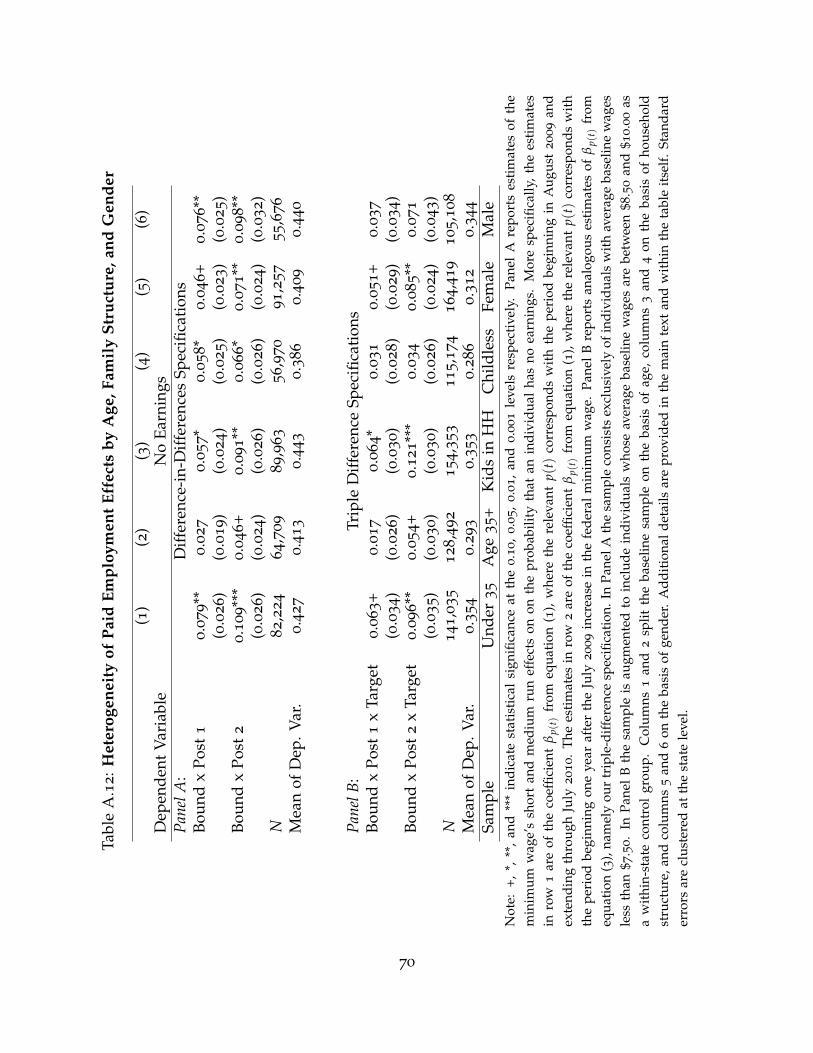
Tabl

eA

.12:H

eter

ogen

eity

ofPa

idEm

ploy

men

tEf

fect

sby

Age

,Fam

ily

Stru

ctur

e,an

dG

ende

r

(1)

(2)

(3)

(4)

(5)

(6)

Dep

ende

ntV

aria

ble

No

Earn

ings

Pane

lA:

Diff

eren

ce-i

n-D

iffer

ence

sSp

ecifi

cati

ons

Boun

dx

Post

10.0

79**

0.0

27

0.0

57*

0.0

58*

0.0

46+

0.0

76**

(0.0

26)

(0.0

19)

(0.0

24)

(0.0

25)

(0.0

23)

(0.0

25)

Boun

dx

Post

20.1

09**

*0.0

46+

0.0

91**

0.0

66*

0.0

71**

0.0

98**

(0.0

26)

(0.0

24)

(0.0

26)

(0.0

26)

(0.0

24)

(0.0

32)

N82,2

24

64,7

09

89,9

63

56,9

70

91,2

57

55,6

76

Mea

nof

Dep

.Var

.0.4

27

0.4

13

0.4

43

0.3

86

0.4

09

0.4

40

Pane

lB:

Trip

leD

iffer

ence

Spec

ifica

tion

sBo

und

xPo

st1

xTa

rget

0.0

63+

0.0

17

0.0

64*

0.0

31

0.0

51+

0.0

37

(0.0

34)

(0.0

26)

(0.0

30)

(0.0

28)

(0.0

29)

(0.0

34)

Boun

dx

Post

2x

Targ

et0.0

96**

0.0

54+

0.1

21**

*0.0

34

0.0

85**

0.0

71

(0.0

35)

(0.0

30)

(0.0

30)

(0.0

26)

(0.0

24)

(0.0

43)

N141,0

35

128,4

92

154,3

53

115,1

74

164,4

19

105,1

08

Mea

nof

Dep

.Var

.0.3

54

0.2

93

0.3

53

0.2

86

0.3

12

0.3

44

Sam

ple

Und

er35

Age

35+

Kid

sin

HH

Chi

ldle

ssFe

mal

eM

ale

Not

e:+,

*,**

,an

d**

*in

dica

test

atis

tica

lsi

gnifi

canc

eat

the

0.1

0,

0.0

5,

0.0

1,

and

0.0

01

leve

lsre

spec

tive

ly.

Pane

lA

repo

rts

esti

mat

esof

the

min

imum

wag

e’s

shor

tan

dm

ediu

mru

nef

fect

son

onth

epr

obab

ility

that

anin

divi

dual

has

noea

rnin

gs.

Mor

esp

ecifi

cally

,th

ees

tim

ates

inro

w1

are

ofth

eco

effic

ient

βp(

t)fr

omeq

uati

on(1

),w

here

the

rele

vant

p(t)

corr

espo

nds

wit

hth

epe

riod

begi

nnin

gin

Aug

ust

2009

and

exte

ndin

gth

roug

hJu

ly2010.

The

esti

mat

esin

row

2ar

eof

the

coef

ficie

ntβ

p(t)

from

equa

tion

(1),

whe

reth

ere

leva

ntp(

t)co

rres

pond

sw

ith

the

peri

odbe

ginn

ing

one

year

afte

rth

eJu

ly2009

incr

ease

inth

efe

dera

lm

inim

umw

age.

Pane

lB

repo

rts

anal

ogou

ses

tim

ates

ofβ

p(t)

from

equa

tion

(3),

nam

ely

our

trip

le-d

iffer

ence

spec

ifica

tion

.In

Pane

lAth

esa

mpl

eco

nsis

tsex

clus

ivel

yof

indi

vidu

als

wit

hav

erag

eba

selin

ew

ages

less

than

$7.5

0.

InPa

nel

Bth

esa

mpl

eis

augm

ente

dto

incl

ude

indi

vidu

als

who

seav

erag

eba

selin

ew

ages

are

betw

een

$8.5

0an

d$1

0.0

0as

aw

ithi

n-st

ate

cont

rol

grou

p.C

olum

ns1

and

2sp

litth

eba

selin

esa

mpl

eon

the

basi

sof

age,

colu

mns

3an

d4

onth

eba

sis

ofho

useh

old

stru

ctur

e,an

dco

lum

ns5

and

6on

the

basi

sof

gend

er.

Add

itio

nald

etai

lsar

epr

ovid

edin

the

mai

nte

xtan

dw

ithi

nth

eta

ble

itse

lf.

Stan

dard

erro

rsar

ecl

uste

red

atth

est

ate

leve

l.

70