the major data mining tasks classification clustering associations most of the other tasks (for...
Post on 20-Dec-2015
222 views
TRANSCRIPT
The Major Data Mining TasksThe Major Data Mining Tasks
• Classification• Clustering• Associations
Most of the other tasks (for example, outlier discovery or anomaly detection ) make heavy use of one or more of the above.
So in this tutorial we will focus most of our energy on the above, starting with…
Grasshoppers
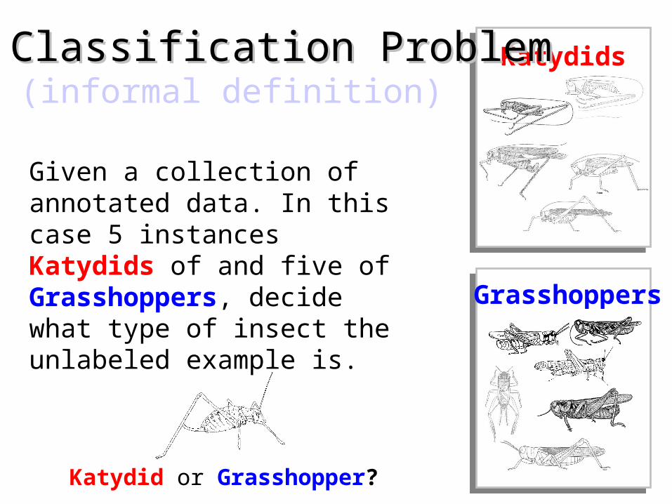
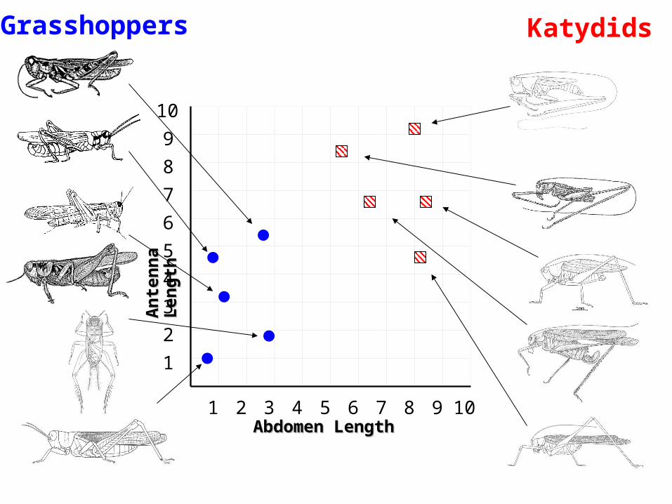
KatydidsThe Classification ProblemThe Classification Problem(informal definition)
Given a collection of annotated data. In this case 5 instances Katydids of and five of Grasshoppers, decide what type of insect the unlabeled example is.
Katydid or Grasshopper?
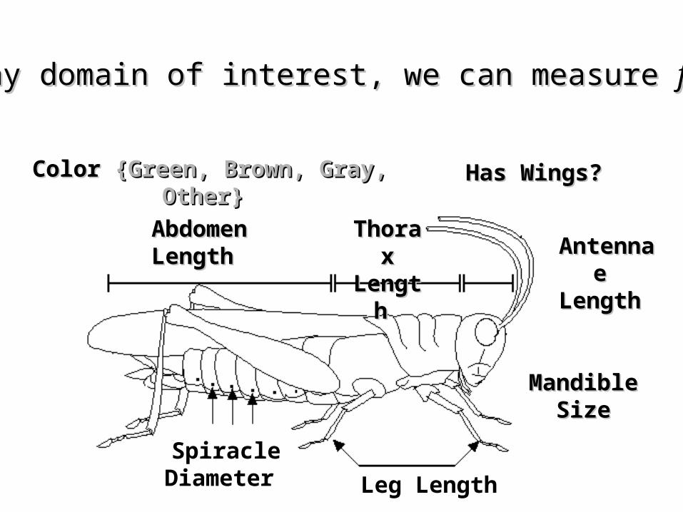
Thorax Thorax LengthLength
Abdomen Abdomen LengthLength Antennae Antennae
LengthLength
MandibleMandibleSizeSize
SpiracleDiameter Leg Length
For any domain of interest, we can measure For any domain of interest, we can measure featuresfeatures
Color Color {Green, Brown, Gray, Other}{Green, Brown, Gray, Other} Has Wings?Has Wings?

Insect Insect IDID
Abdomen Abdomen LengthLength
Antennae Antennae LengthLength
Insect Insect ClassClass
1 2.7 5.5 GrasshopperGrasshopper
2 8.0 9.1 KatydidKatydid
3 0.9 4.7 GrasshopperGrasshopper
4 1.1 3.1 GrasshopperGrasshopper
5 5.4 8.5 KatydidKatydid
6 2.9 1.9 GrasshopperGrasshopper
7 6.1 6.6 KatydidKatydid
8 0.5 1.0 GrasshopperGrasshopper
9 8.3 6.6 KatydidKatydid
10 8.1 4.7 KatydidsKatydids
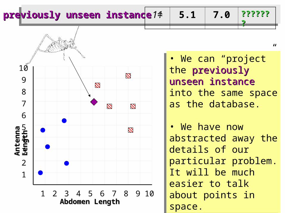
11 5.1 7.0 ??????????????
We can store features We can store features in a database.in a database.
My_CollectionMy_Collection
The classification The classification problem can now be problem can now be expressed as:expressed as:
• Given a training database Given a training database ((My_CollectionMy_Collection), predict ), predict the the class class label of a label of a previously unseen instancepreviously unseen instance
previously unseen instancepreviously unseen instance = =

An
tenn
a L
engt
hA
nte
nna
Len
gth
10
1 2 3 4 5 6 7 8 9 10
1
2
3
4
5
6
7
8
9
Grasshoppers Katydids
Abdomen LengthAbdomen Length
An
tenn
a L
engt
hA
nte
nna
Len
gth
10
1 2 3 4 5 6 7 8 9 10
1
2
3
4
5
6
7
8
9
Grasshoppers Katydids
Abdomen LengthAbdomen Length
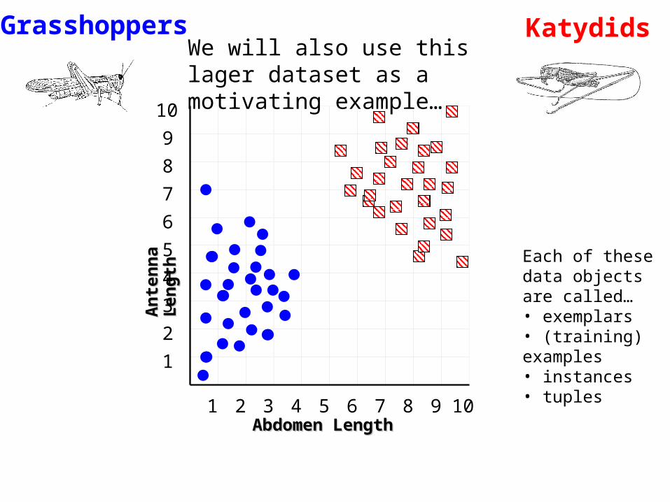
We will also use this lager dataset as a motivating example…
Each of these data objects are called…• exemplars• (training) examples• instances• tuples

We will return to the previous slide in two minutes. In the meantime, we are going to play a quick game.
I am going to show you some classification problems which were shown to pigeons!
Let us see if you are as smart as a pigeon!
We will return to the previous slide in two minutes. In the meantime, we are going to play a quick game.
I am going to show you some classification problems which were shown to pigeons!
Let us see if you are as smart as a pigeon!

Examples of class A
3 4
1.5 5
6 8
2.5 5
Examples of class B
5 2.5
5 2
8 3
4.5 3
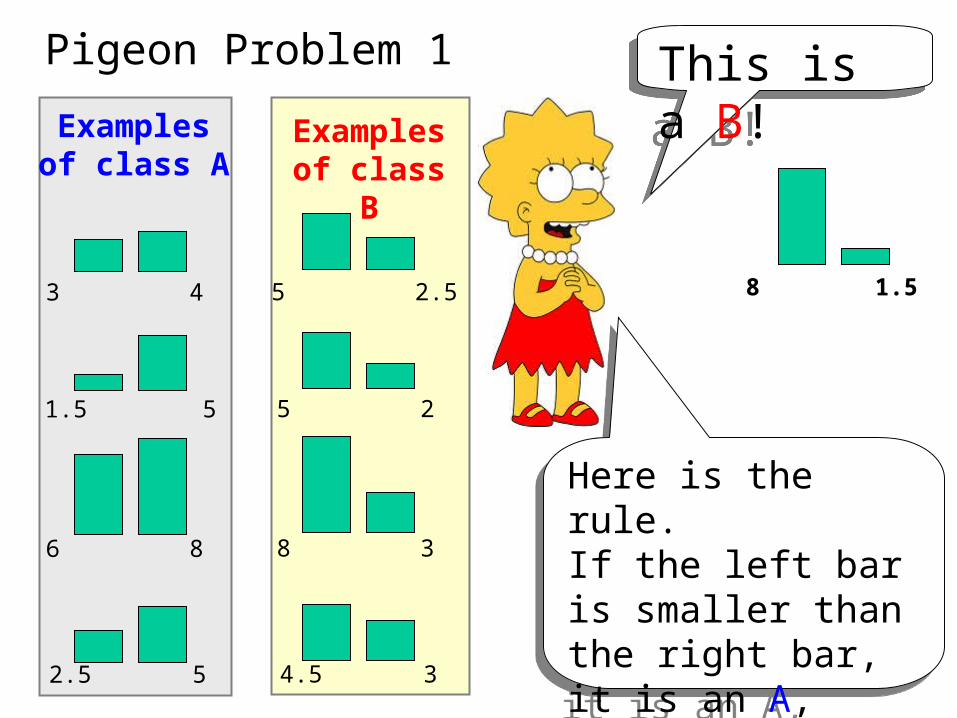
Pigeon Problem 1

Examples of class A
3 4
1.5 5
6 8
2.5 5
Examples of class B
5 2.5
5 2
8 3
4.5 3
8 1.5
4.5 7
What class is this object?
What class is this object?
What about this one, A or B?
What about this one, A or B?
Pigeon Problem 1
Examples of class A
3 4
1.5 5
6 8
2.5 5
Examples of class B
5 2.5
5 2
8 3
4.5 3
8 1.5
This is a B!This is a B!
Pigeon Problem 1
Here is the rule.If the left bar is smaller than the right bar, it is an A, otherwise it is a B.
Here is the rule.If the left bar is smaller than the right bar, it is an A, otherwise it is a B.

Examples of class A
4 4
5 5
6 6
3 3
Examples of class B
5 2.5
2 5
5 3
2.5 3
8 1.5
7 7
Even I know this oneEven I know this one
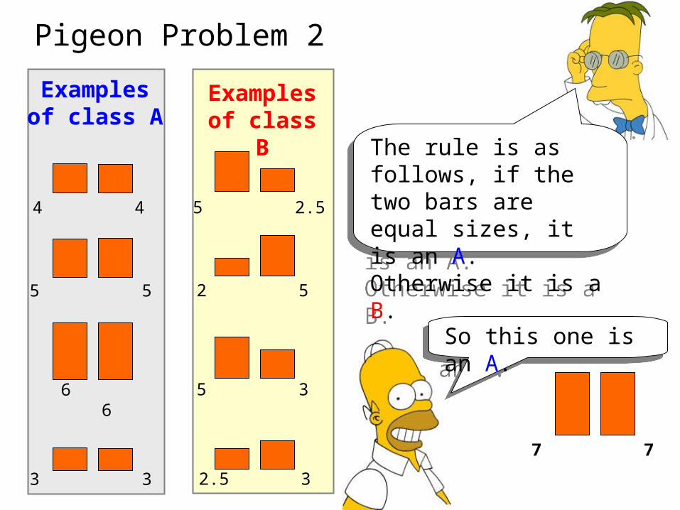
Pigeon Problem 2 Oh! This ones hard!Oh! This ones hard!
Examples of class A
4 4
5 5
6 6
3 3
Examples of class B
5 2.5
2 5
5 3
2.5 3
7 7
Pigeon Problem 2
So this one is an A.So this one is an A.
The rule is as follows, if the two bars are equal sizes, it is an A. Otherwise it is a B.
The rule is as follows, if the two bars are equal sizes, it is an A. Otherwise it is a B.

Examples of class A
4 4
1 5
6 3
3 7
Examples of class B
5 6
7 5
4 8
7 7
6 6
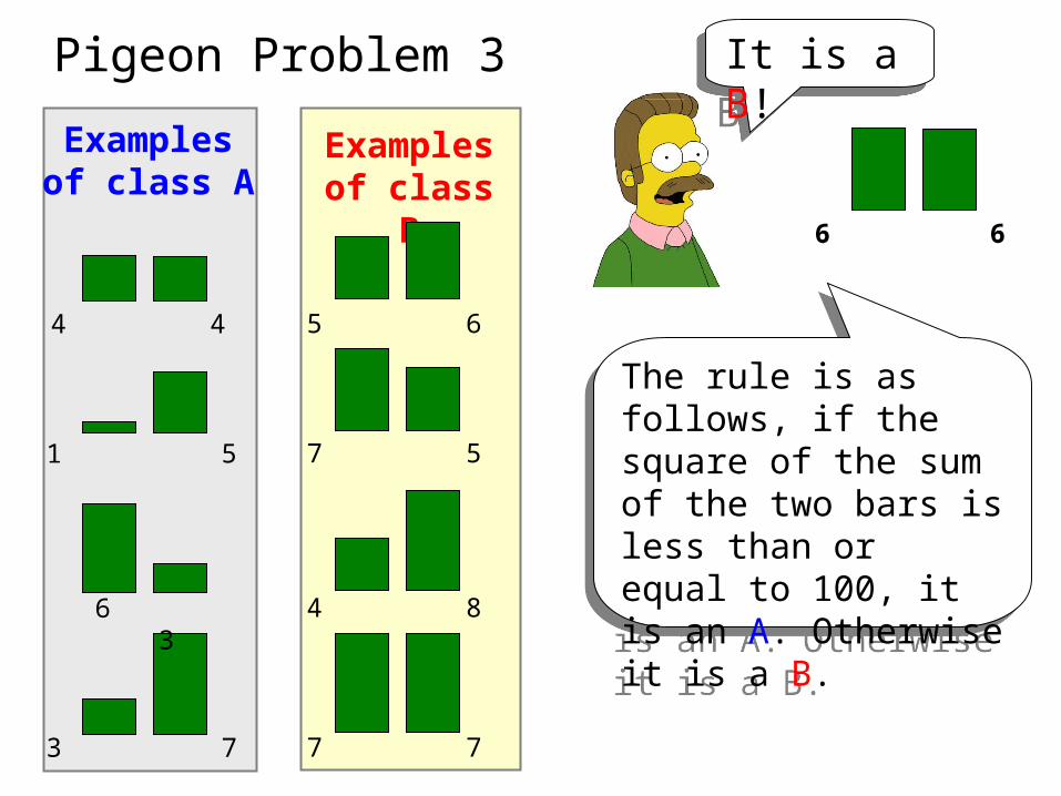
Pigeon Problem 3
This one is really hard!What is this, A or B?
This one is really hard!What is this, A or B?
Examples of class A
4 4
1 5
6 3
3 7
Examples of class B
5 6
7 5
4 8
7 7
6 6
Pigeon Problem 3 It is a B!It is a B!
The rule is as follows, if the square of the sum of the two bars is less than or equal to 100, it is an A. Otherwise it is a B.
The rule is as follows, if the square of the sum of the two bars is less than or equal to 100, it is an A. Otherwise it is a B.

Why did we spend so much time with this game?
Why did we spend so much time with this game?
Because we wanted to show that almost all classification problems have a geometric interpretation, check out the next 3 slides…
Because we wanted to show that almost all classification problems have a geometric interpretation, check out the next 3 slides…

Examples of class A
3 4
1.5 5
6 8
2.5 5
Examples of class B
5 2.5
5 2
8 3
4.5 3
Pigeon Problem 1
Here is the rule again.If the left bar is smaller than the right bar, it is an A, otherwise it is a B.
Here is the rule again.If the left bar is smaller than the right bar, it is an A, otherwise it is a B.
Lef
t B
arL
eft
Bar
10
1 2 3 4 5 6 7 8 9 10
123456789
Right BarRight Bar

Examples of class A
4 4
5 5
6 6
3 3
Examples of class B
5 2.5
2 5
5 3
2.5 3
Pigeon Problem 2
Lef
t B
arL
eft
Bar
10
1 2 3 4 5 6 7 8 9 10
123456789
Right BarRight Bar
Let me look it up… here it is.. the rule is, if the two bars are equal sizes, it is an A. Otherwise it is a B.
Let me look it up… here it is.. the rule is, if the two bars are equal sizes, it is an A. Otherwise it is a B.
Examples of class A
4 4
1 5
6 3
3 7
Examples of class B
5 6
7 5
4 8
7 7
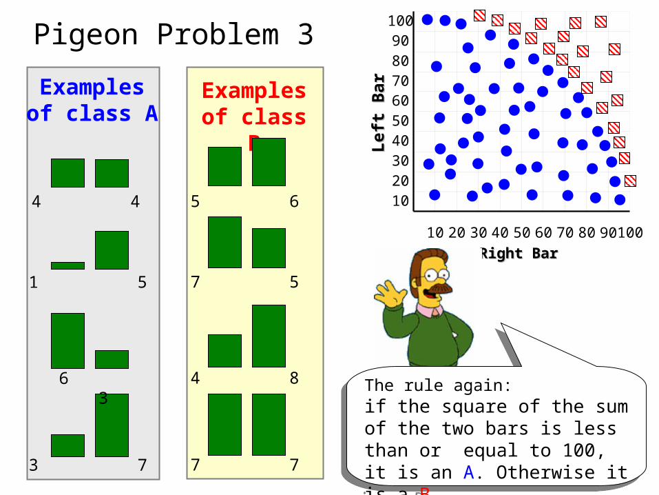
Pigeon Problem 3
Lef
t B
arL
eft
Bar
100
10 20 30 40 50 60 70 80 90 100
102030405060708090
Right BarRight Bar
The rule again:if the square of the sum of the two bars is less than or equal to 100, it is an A. Otherwise it is a B.
The rule again:if the square of the sum of the two bars is less than or equal to 100, it is an A. Otherwise it is a B.
An
tenn
a L
engt
hA
nte
nna
Len
gth
10
1 2 3 4 5 6 7 8 9 10
1
2
3
4
5
6
7
8
9
Grasshoppers Katydids
Abdomen LengthAbdomen Length
An
tenn
a L
engt
hA
nte
nna
Len
gth
10
1 2 3 4 5 6 7 8 9 10
1
2
3
4
5
6
7
8
9
Abdomen LengthAbdomen Length
KatydidsGrasshoppers
• We can “project” the previously unseen instance previously unseen instance into the same space as the database.
• We have now abstracted away the details of our particular problem. It will be much easier to talk about points in space.
• We can “project” the previously unseen instance previously unseen instance into the same space as the database.
• We have now abstracted away the details of our particular problem. It will be much easier to talk about points in space.
11 5.1 7.0 ??????????????previously unseen instancepreviously unseen instance = =

Simple Linear ClassifierSimple Linear Classifier
If previously unseen instancepreviously unseen instance above the linethen class is Katydidelse class is Grasshopper
KatydidsGrasshoppers
R.A. Fisher1890-1962
10
1 2 3 4 5 6 7 8 9 10
1
2
3
4
5
6
7
8
9
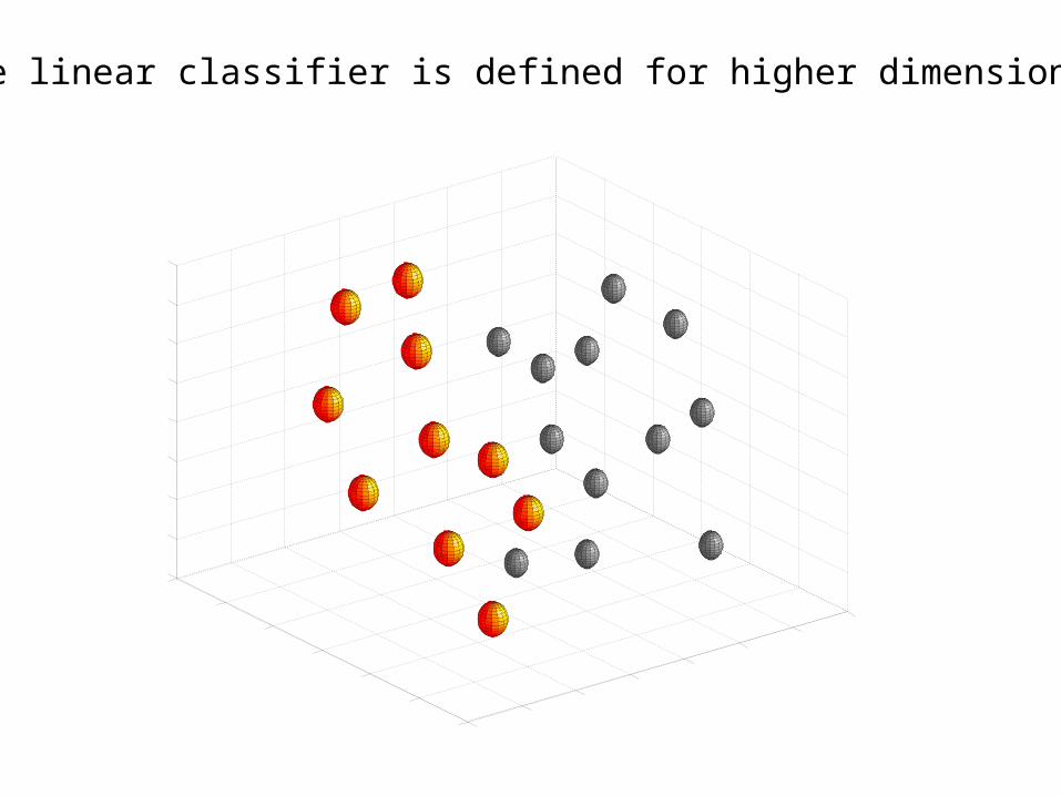
The simple linear classifier is defined for higher dimensional spaces…
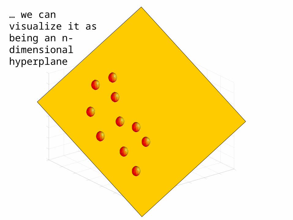
… we can visualize it as being an n-dimensional hyperplane
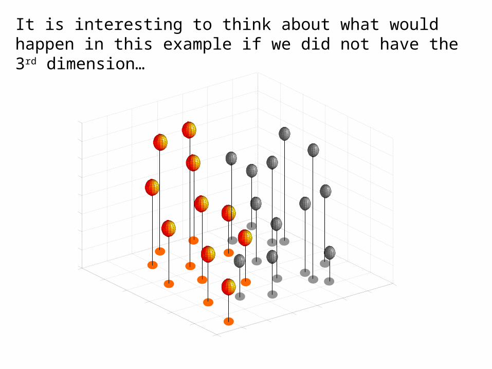
It is interesting to think about what would happen in this example if we did not have the 3rd dimension…

We can no longer get perfect accuracy with the simple linear classifier…
We could try to solve this problem by user a simple quadratic classifier or a simple cubic classifier..
However, as we will later see, this is probably a bad idea…

10
1 2 3 4 5 6 7 8 9 10
123456789
100
10 20 30 40 50 60 70 80 90 100
10
20
30
40
50
60
70
80
90
10
1 2 3 4 5 6 7 8 9 10
123456789
Which of the “Pigeon Problems” can be Which of the “Pigeon Problems” can be solved by the Simple Linear Classifier?solved by the Simple Linear Classifier?
1)1) PerfectPerfect2)2) UselessUseless3)3) Pretty GoodPretty Good
Problems that can be solved by a linear classifier are call linearly separable.

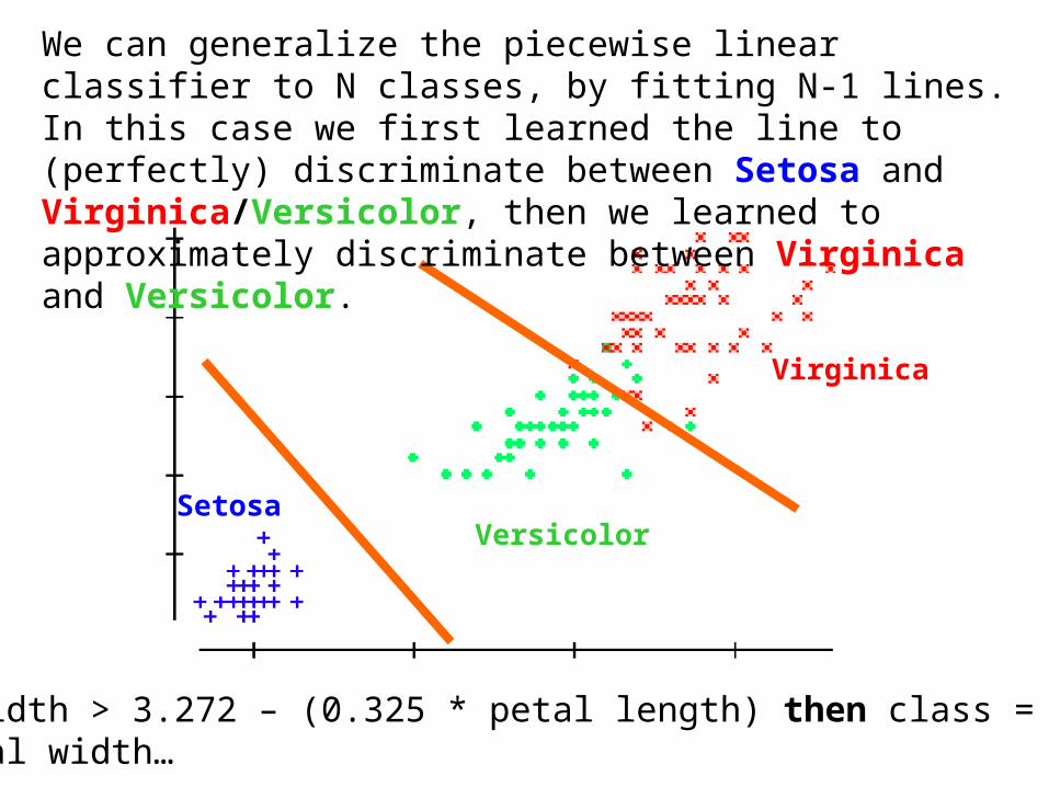
A Famous ProblemA Famous ProblemR. A. Fisher’s Iris Dataset.
• 3 classes
• 50 of each class
The task is to classify Iris plants into one of 3 varieties using the Petal Length and Petal Width.
Iris Setosa Iris Versicolor Iris Virginica
Setosa
Versicolor
Virginica
SetosaVersicolor
Virginica
We can generalize the piecewise linear classifier to N classes, by fitting N-1 lines. In this case we first learned the line to (perfectly) discriminate between Setosa and Virginica/Versicolor, then we learned to approximately discriminate between Virginica and Versicolor.
If petal width > 3.272 – (0.325 * petal length) then class = VirginicaElseif petal width…
• Predictive accuracy• Speed and scalability
– time to construct the model– time to use the model– efficiency in disk-resident databases
• Robustness– handling noise, missing values and irrelevant features,
streaming data• Interpretability:
– understanding and insight provided by the model
We have now seen one classification We have now seen one classification algorithm, and we are about to see more. algorithm, and we are about to see more. How should we compare themHow should we compare them??
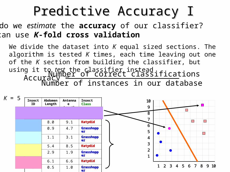
Predictive Accuracy IPredictive Accuracy I• How do we estimate the accuracy of our classifier?
We can use K-fold cross validation
Insect IDInsect ID Abdomen Abdomen LengthLength
Antennae Antennae LengthLength
Insect Insect ClassClass
1 2.7 5.5 GrasshopperGrasshopper
2 8.0 9.1 KatydidKatydid
3 0.9 4.7 GrasshopperGrasshopper
4 1.1 3.1 GrasshopperGrasshopper
5 5.4 8.5 KatydidKatydid
6 2.9 1.9 GrasshopperGrasshopper
7 6.1 6.6 KatydidKatydid
8 0.5 1.0 GrasshopperGrasshopper
9 8.3 6.6 KatydidKatydid
10 8.1 4.7 KatydidsKatydids
We divide the dataset into K equal sized sections. The algorithm is tested K times, each time leaving out one of the K section from building the classifier, but using it to test the classifier instead
10
1 2 3 4 5 6 7 8 9 10
1
2
3
4
5
6
7
8
9
10
1 2 3 4 5 6 7 8 9 10
1
2
3
4
5
6
7
8
9
10
1 2 3 4 5 6 7 8 9 10
1
2
3
4
5
6
7
8
9
Accuracy = Number of correct classificationsNumber of instances in our database
K = 5
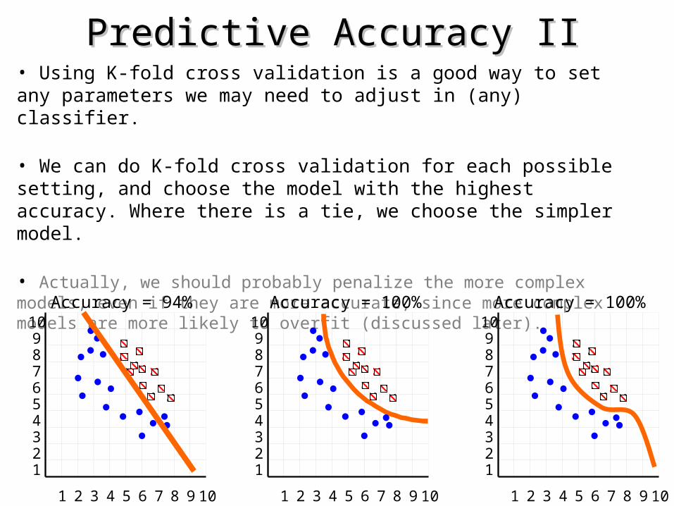
Predictive Accuracy IIPredictive Accuracy II• Using K-fold cross validation is a good way to set any parameters we may need to adjust in (any) classifier.
• We can do K-fold cross validation for each possible setting, and choose the model with the highest accuracy. Where there is a tie, we choose the simpler model.
• Actually, we should probably penalize the more complex models, even if they are more accurate, since more complex models are more likely to overfit (discussed later).
10
1 2 3 4 5 6 7 8 9 10
123456789
10
1 2 3 4 5 6 7 8 9 10
123456789
10
1 2 3 4 5 6 7 8 9 10
123456789
Accuracy = 94% Accuracy = 100% Accuracy = 100%
Predictive Accuracy IIIPredictive Accuracy III
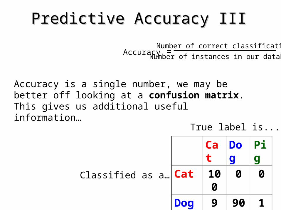
Accuracy = Number of correct classifications
Number of instances in our database
Accuracy is a single number, we may be better off looking at a confusion matrix. This gives us additional useful information…
Cat Dog Pig
Cat 100 0 0
Dog 9 90 1
Pig 45 45 10
Classified as a…
True label is...
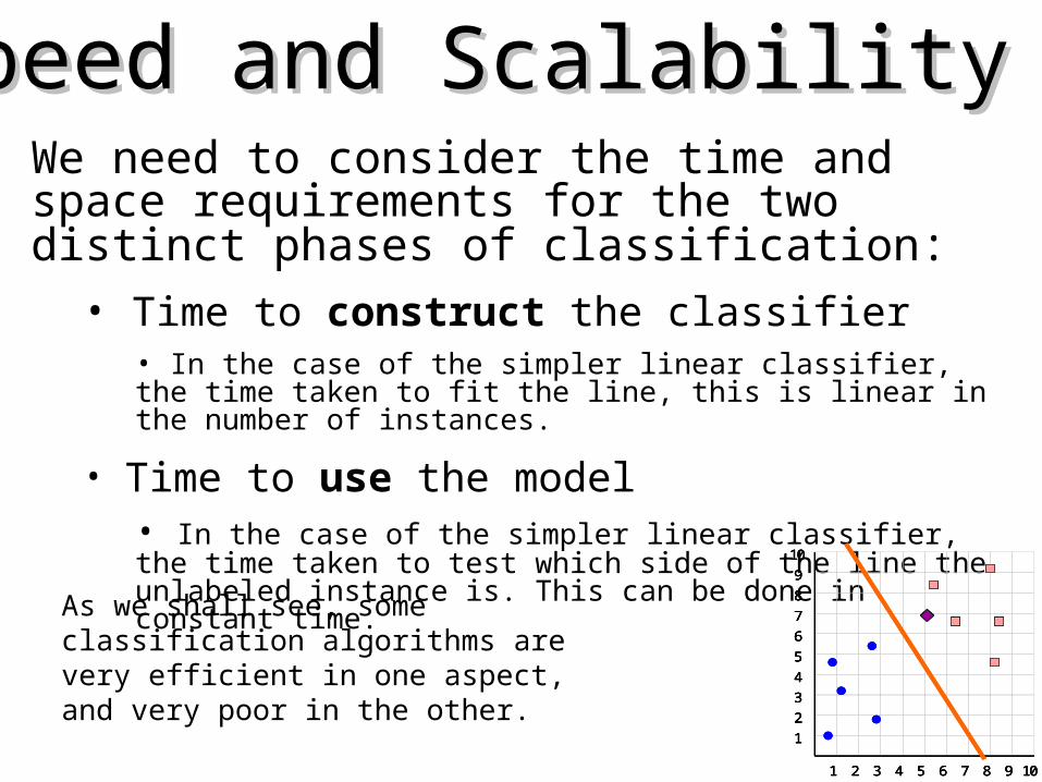
We need to consider the time and space requirements for the two distinct phases of classification:
• Time to construct the classifier• In the case of the simpler linear classifier, the time taken to fit the line, this is linear in the number of instances.
• Time to use the model• In the case of the simpler linear classifier, the time taken to test which side of the line the unlabeled instance is. This can be done in constant time.
Speed and Scalability ISpeed and Scalability I
10
1 2 3 4 5 6 7 8 9 10
1
2
3
4
5
6
7
8
9
10
1 2 3 4 5 6 7 8 9 10
1
2
3
4
5
6
7
8
9
10
1 2 3 4 5 6 7 8 9 10
1
2
3
4
5
6
7
8
9
10
1 2 3 4 5 6 7 8 9 10
1
2
3
4
5
6
7
8
9
As we shall see, some classification algorithms are very efficient in one aspect, and very poor in the other.

Speed and Scalability IISpeed and Scalability IIWe need to consider the time and space requirements for the two distinct phases of classification:
•Time to construct the classifier•In the case of the simpler linear classifier, the time taken to fit the line, this is linear in the number of instances.
•Time to usethe model• In the case of the simpler linear classifier, the time taken to test which side of the line the unlabeled instance is. This can be done in constant time.
Speed and Scalability ISpeed and Scalability I
10
1 2 3 4 5 6 7 8 9 10
1
2
3
4
5
6
7
8
9
10
1 2 3 4 5 6 7 8 9 10
1
2
3
4
5
6
7
8
9
10
1 2 3 4 5 6 7 8 9 10
1
2
3
4
5
6
7
8
9
10
1 2 3 4 5 6 7 8 9 10
1
2
3
4
5
6
7
8
9
As we shall see, some classification algorithms are very efficient in one aspect, and very poor in the other.
For learning with small datasets, this is the whole picture
However, for data mining with massive datasets, it is not so much the (main memory) time complexity that matters, rather it is how many times we have to scan the database.
This is because for most data mining operations, disk access times completely dominate the CPU times.
For data mining, researchers often report the number of times you must scan the database.
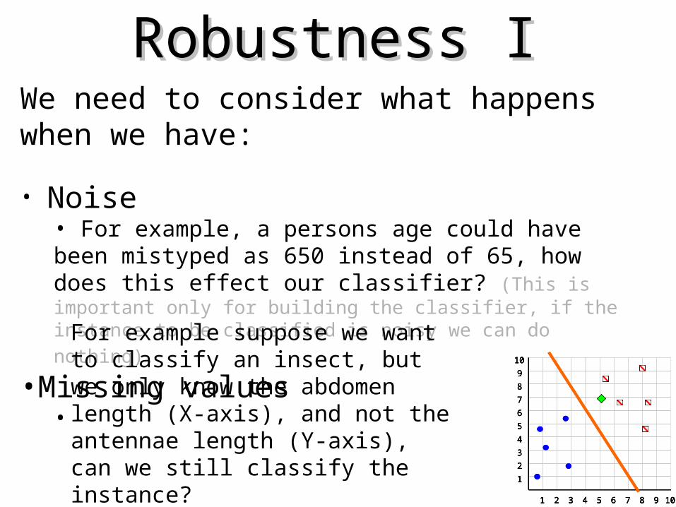
Robustness IRobustness IWe need to consider what happens when we have:
• Noise• For example, a persons age could have been mistyped as 650 instead of 65, how does this effect our classifier? (This is important only for building the classifier, if the instance to be classified is noisy we can
do nothing).
•Missing values•
10
1 2 3 4 5 6 7 8 9 10
1
2
3
4
5
6
7
8
9
10
1 2 3 4 5 6 7 8 9 10
1
2
3
4
5
6
7
8
9
10
1 2 3 4 5 6 7 8 9 10
1
2
3
4
5
6
7
8
9
10
1 2 3 4 5 6 7 8 9 10
1
2
3
4
5
6
7
8
9
For example suppose we want to classify an insect, but we only know the abdomen length (X-axis), and not the antennae length (Y-axis), can we still classify the instance?
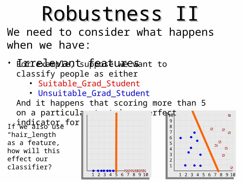
Robustness IIRobustness IIWe need to consider what happens when we have:
• Irrelevant featuresFor example, suppose we want to classify people as either
• Suitable_Grad_Student• Unsuitable_Grad_Student
And it happens that scoring more than 5 on a particular test is a perfect indicator for this problem…
1 2 3 4 5 6 7 8 9 10 1 2 3 4 5 6 7 8 9 10
123456789
10
If we also use “hair_length” as a feature, how will this effect our classifier?

Robustness IIIRobustness IIIWe need to consider what happens when we have:
• Streaming dataFor many real world problems, we don’t have a single fixed dataset. Instead, the data continuously arrives, potentially forever… (stock market, weather data, sensor data etc)
1 2 3 4 5 6 7 8 9 10
123456789
10
Can our classifier handle streaming data?
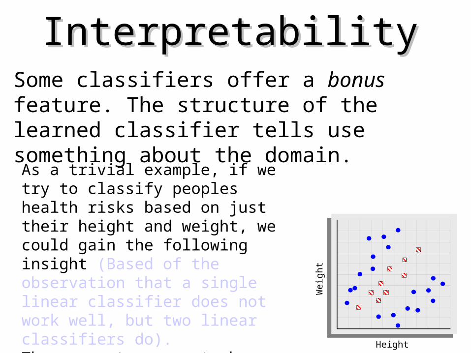
InterpretabilityInterpretabilitySome classifiers offer a bonus feature. The structure of the learned classifier tells use something about the domain.
Height
Wei
ght
As a trivial example, if we try to classify peoples health risks based on just their height and weight, we could gain the following insight (Based of the observation that a single linear classifier does not work well, but two linear classifiers do).There are two ways to be unhealthy, being obese and being too skinny.

Nearest Neighbor ClassifierNearest Neighbor Classifier
If the nearest instance to the previously previously unseen instance unseen instance is a Katydid class is Katydidelse class is Grasshopper
KatydidsGrasshoppers
Joe Hodges 1922-2000
Evelyn Fix 1904-1965
An
tenn
a L
engt
hA
nte
nna
Len
gth
10
1 2 3 4 5 6 7 8 9 10
1
2
3
4
5
6
7
8
9
Abdomen LengthAbdomen Length
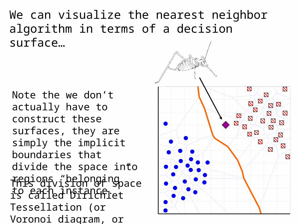
This division of space is called Dirichlet Tessellation (or Voronoi diagram, or Theissen regions).
We can visualize the nearest neighbor algorithm in terms of a decision surface…
Note the we don’t actually have to construct these surfaces, they are simply the implicit boundaries that divide the space into regions “belonging” to each instance.
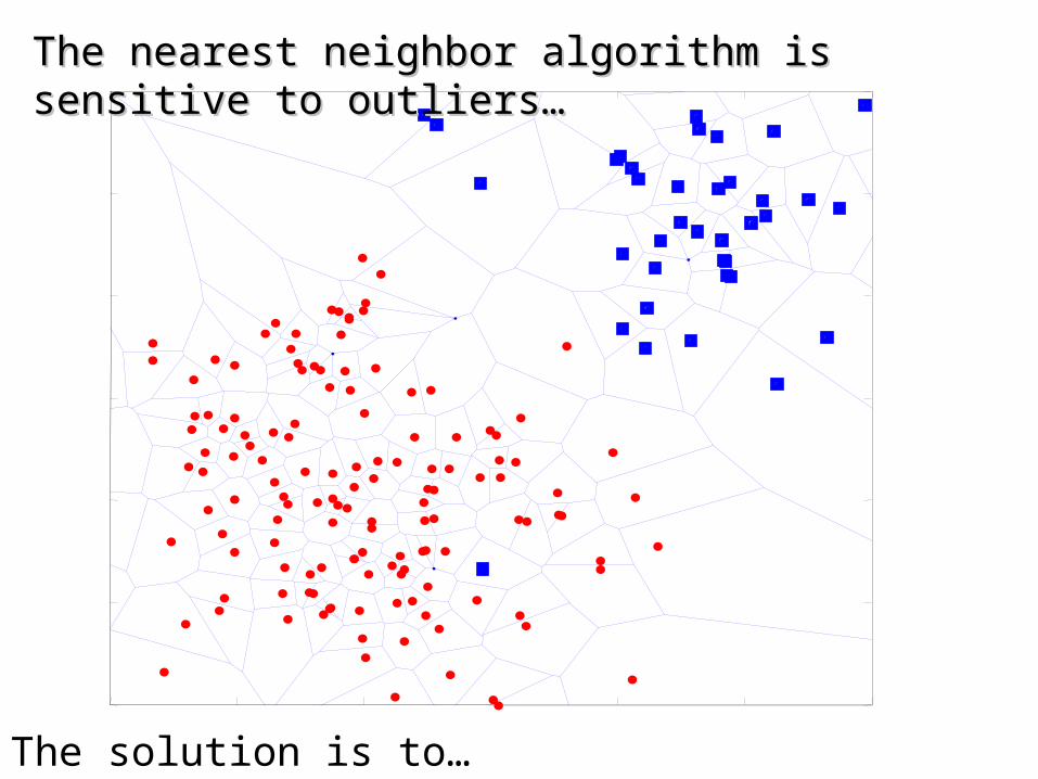
The nearest neighbor algorithm is sensitive to outliers…The nearest neighbor algorithm is sensitive to outliers…
The solution is to…
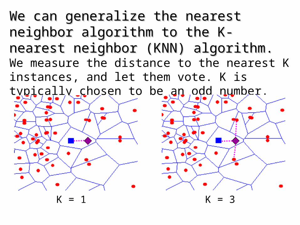
We can generalize the nearest neighbor algorithm to We can generalize the nearest neighbor algorithm to the K- nearest neighbor (KNN) algorithm. the K- nearest neighbor (KNN) algorithm. We measure the distance to the nearest K instances, and let them vote. K is typically chosen to be an odd number.
K = 1 K = 3
1 2 3 4 5 6 7 8 9 10 1 2 3 4 5 6 7 8 9 10
123456789
10
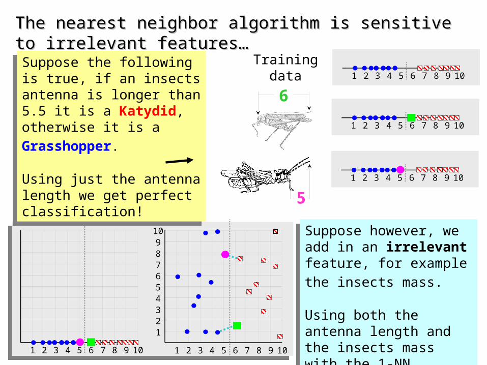
1 2 3 4 5 6 7 8 9 10Suppose the following is true, if an insects antenna is longer than 5.5 it is a Katydid, otherwise it
is a Grasshopper.
Using just the antenna length we get perfect classification!
Suppose the following is true, if an insects antenna is longer than 5.5 it is a Katydid, otherwise it
is a Grasshopper.
Using just the antenna length we get perfect classification!
The nearest neighbor algorithm is sensitive to irrelevant features…The nearest neighbor algorithm is sensitive to irrelevant features…
Training data
1 2 3 4 5 6 7 8 9 10
1 2 3 4 5 6 7 8 9 10
6
5
Suppose however, we add in an irrelevant feature, for
example the insects mass.
Using both the antenna length and the insects mass with the 1-NN algorithm we get the wrong classification!
Suppose however, we add in an irrelevant feature, for
example the insects mass.
Using both the antenna length and the insects mass with the 1-NN algorithm we get the wrong classification!

How do we mitigate the nearest neighbor How do we mitigate the nearest neighbor algorithms sensitivity to irrelevant features? algorithms sensitivity to irrelevant features?
• Use more training instances
• Ask an expert what features are relevant to the task
• Use statistical tests to try to determine which features are useful
• Search over feature subsets (in the next slide we will see why this is hard)
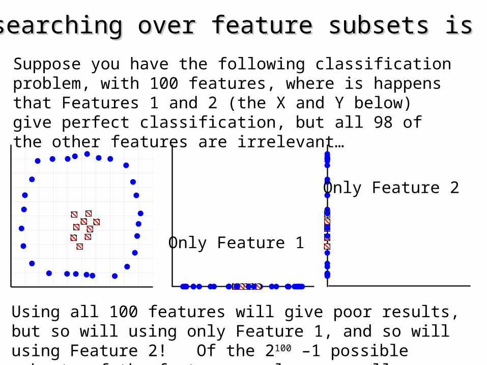
Why searching over feature subsets is hardWhy searching over feature subsets is hard
Suppose you have the following classification problem, with 100 features, where is happens that Features 1 and 2 (the X and Y below) give perfect classification, but all 98 of the other features are irrelevant…
Using all 100 features will give poor results, but so will using only Feature 1, and so will using Feature 2! Of the 2100 –1 possible subsets of the features, only one really works.
Only Feature 1
Only Feature 2
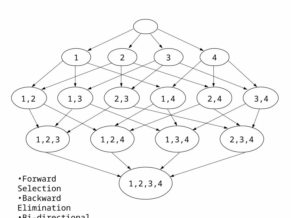
1 2 3 4
3,42,41,42,31,31,2
2,3,41,3,41,2,41,2,3
1,2,3,4•Forward Selection•Backward Elimination•Bi-directional Search

The nearest neighbor algorithm is sensitive to the units of measurementThe nearest neighbor algorithm is sensitive to the units of measurement
X axis measured in centimetersY axis measure in dollars
The nearest neighbor to the pink unknown instance is red.
X axis measured in millimetersY axis measure in dollars
The nearest neighbor to the pink unknown instance is blue.
One solution is to normalize the units to pure numbers. Typically the features are Z-normalized to have a mean of zero and a standard deviation of one. X = (X – mean(X))/std(x)

We can speed up nearest neighbor algorithm by “throwing We can speed up nearest neighbor algorithm by “throwing away” some data. This is called data editing.away” some data. This is called data editing.Note that this can sometimes improve accuracy!Note that this can sometimes improve accuracy!
One possible approach. Delete all instances that are surrounded by members of their own class.
We can also speed up classification with indexing
10
1 2 3 4 5 6 7 8 9 10
1
2
3
4
5
6
7
8
9
pn
i
pii cqCQD
1,
n
iii cqCQD
1
2,
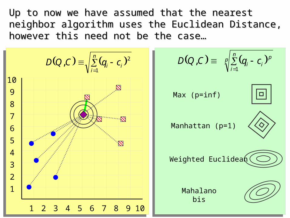
Manhattan (p=1)
Max (p=inf)
Mahalanobis
Weighted Euclidean
Up to now we have assumed that the nearest neighbor algorithm uses Up to now we have assumed that the nearest neighbor algorithm uses the Euclidean Distance, however this need not be the case…the Euclidean Distance, however this need not be the case…

……In fact, we can use the nearest neighbor algorithm with In fact, we can use the nearest neighbor algorithm with any distance/similarity function any distance/similarity function
IDID NameName ClassClass
1 Gunopulos GreekGreek
2 Papadopoulos GreekGreek
3 Kollios GreekGreek
4 Dardanos GreekGreek
5 Keogh IrishIrish
6 Gough IrishIrish
7 Greenhaugh IrishIrish
8 Hadleigh IrishIrish
For example, is “Faloutsos” Greek or Irish? We could compare the name “Faloutsos” to a database of names using string edit distance…
edit_distance(Faloutsos, Keogh) = 8edit_distance(Faloutsos, Gunopulos) = 6
Hopefully, the similarity of the name (particularly the suffix) to other Greek names would mean the nearest nearest neighbor is also a Greek name.
Specialized distance measures exist for DNA strings, time series, images, graphs, videos, sets, fingerprints etc…

• Advantages:– Simple to implement– Handles correlated features (Arbitrary class shapes)
– Defined for any distance measure– Handles streaming data trivially
• Disadvantages:– Very sensitive to irrelevant features.– Slow classification time for large datasets– Works best for real valued datasets
Advantages/Disadvantages of Nearest NeighborAdvantages/Disadvantages of Nearest Neighbor

Decision Tree ClassifierDecision Tree Classifier
Ross Quinlan
An
tenn
a L
engt
hA
nte
nna
Len
gth
10
1 2 3 4 5 6 7 8 9 10
1
2
3
4
5
6
7
8
9
Abdomen LengthAbdomen Length
Abdomen LengthAbdomen Length > 7.1?
no yes
KatydidAntenna LengthAntenna Length > 6.0?
no yes
KatydidGrasshopper
Grasshopper
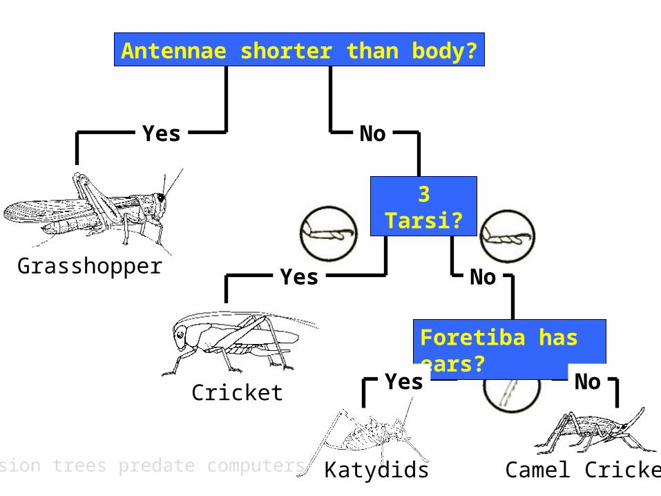
Antennae shorter than body?
Cricket
Foretiba has ears?
Katydids Camel Cricket
Yes
Yes
Yes
No
No
3 Tarsi?
No
Decision trees predate computers
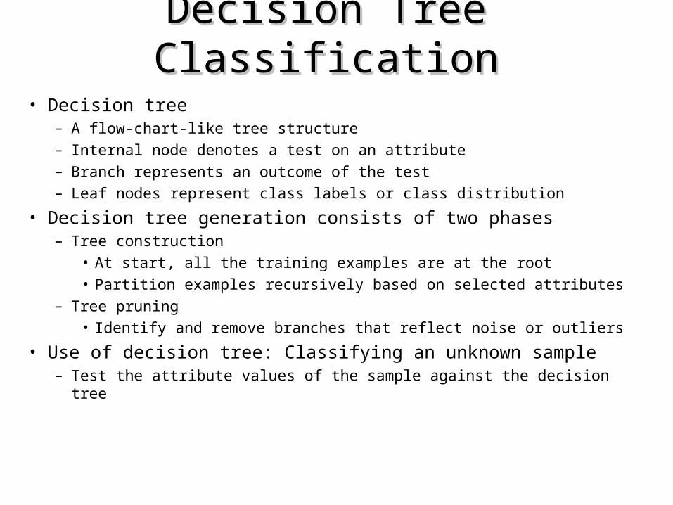
• Decision tree – A flow-chart-like tree structure
– Internal node denotes a test on an attribute
– Branch represents an outcome of the test
– Leaf nodes represent class labels or class distribution
• Decision tree generation consists of two phases– Tree construction
• At start, all the training examples are at the root
• Partition examples recursively based on selected attributes
– Tree pruning
• Identify and remove branches that reflect noise or outliers
• Use of decision tree: Classifying an unknown sample– Test the attribute values of the sample against the decision tree
Decision Tree ClassificationDecision Tree Classification
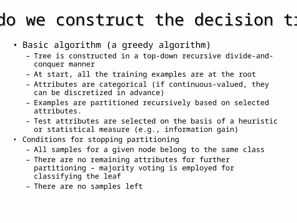
• Basic algorithm (a greedy algorithm)– Tree is constructed in a top-down recursive divide-and-conquer manner– At start, all the training examples are at the root– Attributes are categorical (if continuous-valued, they can be discretized
in advance)– Examples are partitioned recursively based on selected attributes.– Test attributes are selected on the basis of a heuristic or statistical
measure (e.g., information gain)• Conditions for stopping partitioning
– All samples for a given node belong to the same class– There are no remaining attributes for further partitioning – majority
voting is employed for classifying the leaf– There are no samples left
How do we construct the decision tree?How do we construct the decision tree?
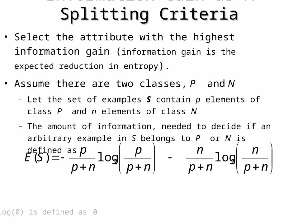
Information Gain as A Splitting CriteriaInformation Gain as A Splitting Criteria• Select the attribute with the highest information gain (information
gain is the expected reduction in entropy).
• Assume there are two classes, P and N
– Let the set of examples S contain p elements of class P and n elements of
class N
– The amount of information, needed to decide if an arbitrary example in S
belongs to P or N is defined as
np
n
np
n
np
p
np
pSE 22 loglog)(
0 log(0) is defined as 0

Information Gain in Decision Tree InductionInformation Gain in Decision Tree Induction
• Assume that using attribute A, a current set will be partitioned into some number of child sets
• The encoding information that would be gained by branching on A
)()()( setschildallEsetCurrentEAGain
Note: entropy is at its minimum if the collection of objects is completely uniform
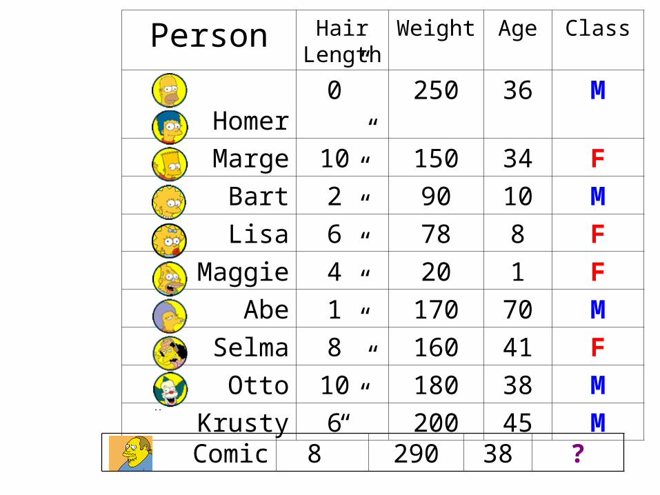
Person Hair Length
Weight Age Class
Homer 0” 250 36 M
Marge 10” 150 34 F
Bart 2” 90 10 M
Lisa 6” 78 8 F
Maggie 4” 20 1 F
Abe 1” 170 70 M
Selma 8” 160 41 F
Otto 10” 180 38 M
Krusty 6” 200 45 M
Comic 8” 290 38 ?

Hair Length <= 5?yes no
Entropy(4F,5M) = -(4/9)log2(4/9) - (5/9)log2(5/9) = 0.9911
Entropy(1F,3M) = -(1/4)log2(1/4) - (3/4)log
2(3/4)
= 0.8113
Entropy(3F,2M) = -(3/5)log2(3/5) - (2/5)log
2(2/5)
= 0.9710
np
n
np
n
np
p
np
pSEntropy 22 loglog)(
Gain(Hair Length <= 5) = 0.9911 – (4/9 * 0.8113 + 5/9 * 0.9710 ) = 0.0911
)()()( setschildallEsetCurrentEAGain
Let us try splitting on Hair length
Let us try splitting on Hair length

Weight <= 160?yes no
Entropy(4F,5M) = -(4/9)log2(4/9) - (5/9)log2(5/9) = 0.9911
Entropy(4F,1M) = -(4/5)log2(4/5) - (1/5)log
2(1/5)
= 0.7219
Entropy(0F,4M) = -(0/4)log2(0/4) - (4/4)log
2(4/4)
= 0
np
n
np
n
np
p
np
pSEntropy 22 loglog)(
Gain(Weight <= 160) = 0.9911 – (5/9 * 0.7219 + 4/9 * 0 ) = 0.5900
)()()( setschildallEsetCurrentEAGain
Let us try splitting on Weight
Let us try splitting on Weight
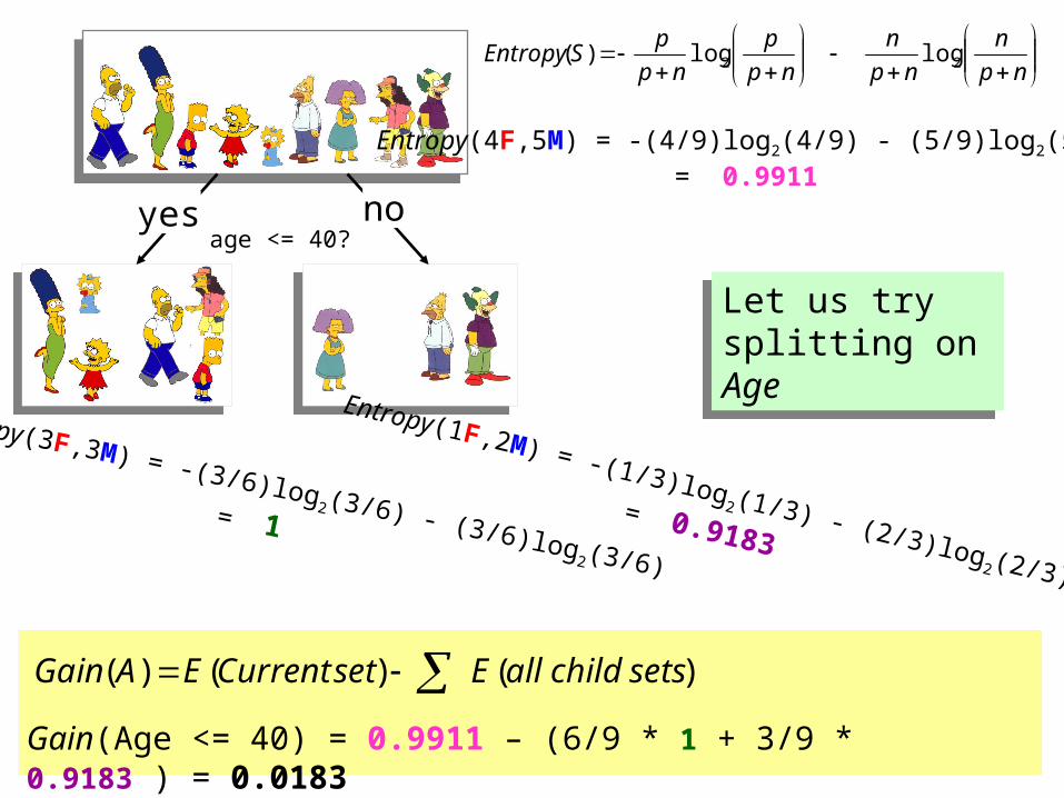
age <= 40?yes no
Entropy(4F,5M) = -(4/9)log2(4/9) - (5/9)log2(5/9) = 0.9911
Entropy(3F,3M) = -(3/6)log2(3/6) - (3/6)log
2(3/6)
= 1
Entropy(1F,2M) = -(1/3)log2(1/3) - (2/3)log
2(2/3)
= 0.9183
np
n
np
n
np
p
np
pSEntropy 22 loglog)(
Gain(Age <= 40) = 0.9911 – (6/9 * 1 + 3/9 * 0.9183 ) = 0.0183
)()()( setschildallEsetCurrentEAGain
Let us try splitting on Age
Let us try splitting on Age
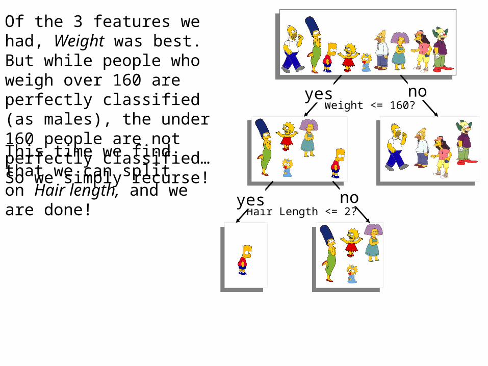
Weight <= 160?yes no
Hair Length <= 2?yes no
Of the 3 features we had, Weight was best. But while people who weigh over 160 are perfectly classified (as males), the under 160 people are not perfectly classified… So we simply recurse!
This time we find that we can split on Hair length, and we are done!

Weight <= 160?
yes no
Hair Length <= 2?
yes no
We need don’t need to keep the data around, just the test conditions.
Male
Male Female
How would these people be classified?

It is trivial to convert Decision Trees to rules…
Weight <= 160?
yes no
Hair Length <= 2?
yes no
Male
Male Female
Rules to Classify Males/Females
If Weight greater than 160, classify as MaleElseif Hair Length less than or equal to 2, classify as MaleElse classify as Female
Rules to Classify Males/Females
If Weight greater than 160, classify as MaleElseif Hair Length less than or equal to 2, classify as MaleElse classify as Female

Decision tree for a typical shared-care setting applying Decision tree for a typical shared-care setting applying the system for the diagnosis of prostatic obstructions.the system for the diagnosis of prostatic obstructions.
Once we have learned the decision tree, we don’t even need a computer!Once we have learned the decision tree, we don’t even need a computer!
This decision tree is attached to a medical machine, and is designed to help
nurses make decisions about what type of doctor to call.
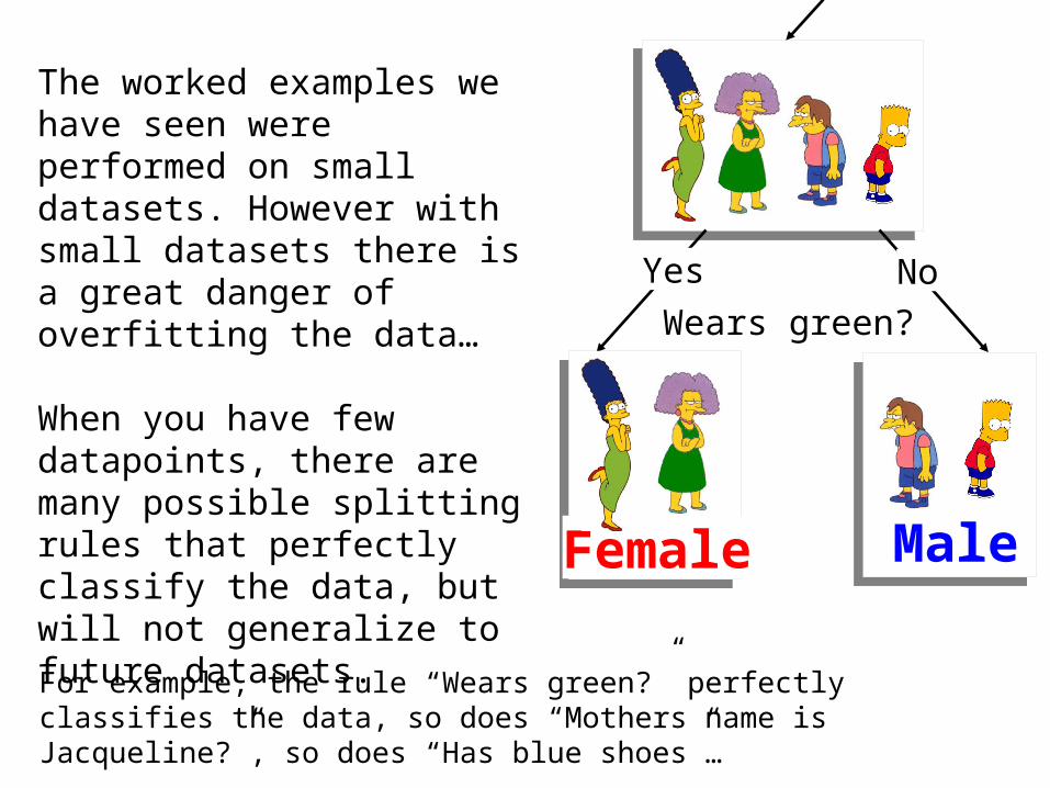
Wears green?
Yes No
The worked examples we have seen were performed on small datasets. However with small datasets there is a great danger of overfitting the data…
When you have few datapoints, there are many possible splitting rules that perfectly classify the data, but will not generalize to future datasets.
For example, the rule “Wears green?” perfectly classifies the data, so does “Mothers name is Jacqueline?”, so does “Has blue shoes”…
MaleFemale
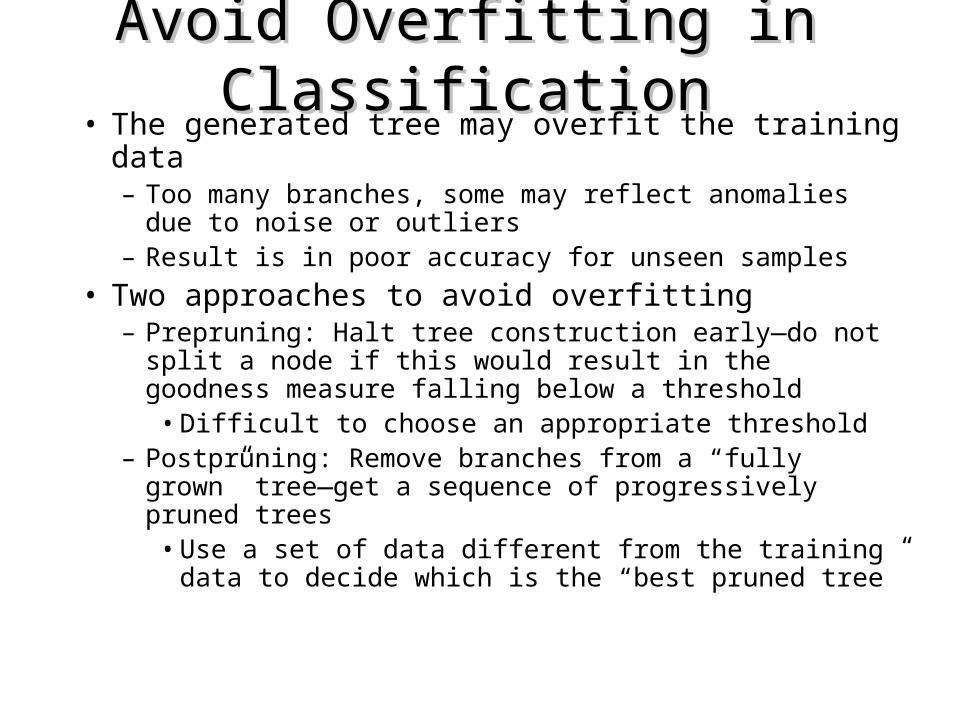
Avoid Overfitting in ClassificationAvoid Overfitting in Classification• The generated tree may overfit the training data
– Too many branches, some may reflect anomalies due to noise or outliers
– Result is in poor accuracy for unseen samples
• Two approaches to avoid overfitting – Prepruning: Halt tree construction early—do not split a
node if this would result in the goodness measure falling below a threshold
• Difficult to choose an appropriate threshold– Postpruning: Remove branches from a “fully grown” tree
—get a sequence of progressively pruned trees• Use a set of data different from the training data to
decide which is the “best pruned tree”
10
1 2 3 4 5 6 7 8 9 10
123456789
100
10 20 30 40 50 60 70 80 90 100
10
20
30
40
50
60
70
80
90
10
1 2 3 4 5 6 7 8 9 10
123456789
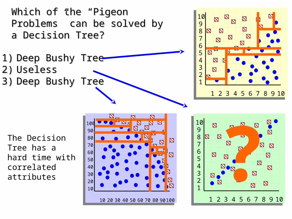
Which of the “Pigeon Problems” can be Which of the “Pigeon Problems” can be solved by a Decision Tree?solved by a Decision Tree?
1)1) Deep Bushy TreeDeep Bushy Tree2)2) UselessUseless3)3) Deep Bushy TreeDeep Bushy Tree
The Decision Tree has a hard time with correlated attributes ?
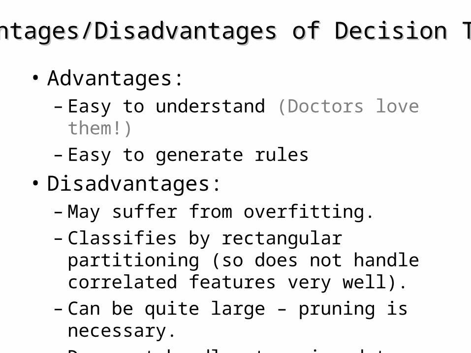
• Advantages:– Easy to understand (Doctors love them!) – Easy to generate rules
• Disadvantages:– May suffer from overfitting.– Classifies by rectangular partitioning (so does
not handle correlated features very well).– Can be quite large – pruning is necessary.– Does not handle streaming data easily
Advantages/Disadvantages of Decision TreesAdvantages/Disadvantages of Decision Trees
Naïve Bayes ClassifierNaïve Bayes Classifier
We will start off with a visual intuition, before looking at the math…
Thomas Bayes1702 - 1761
An
tenn
a L
engt
hA
nte
nna
Len
gth
10
1 2 3 4 5 6 7 8 9 10
1
2
3
4
5
6
7
8
9
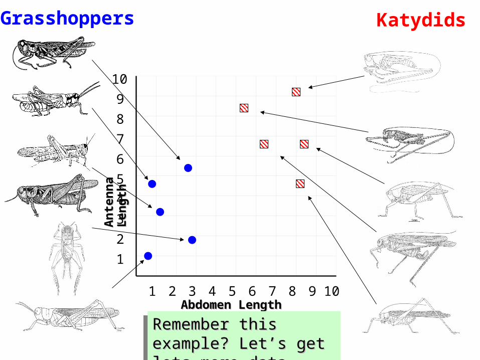
Grasshoppers Katydids
Abdomen LengthAbdomen Length
Remember this example? Remember this example? Let’s get lots more data…Let’s get lots more data…
Remember this example? Remember this example? Let’s get lots more data…Let’s get lots more data…
An
tenn
a L
engt
hA
nte
nna
Len
gth
10
1 2 3 4 5 6 7 8 9 10
1
2
3
4
5
6
7
8
9
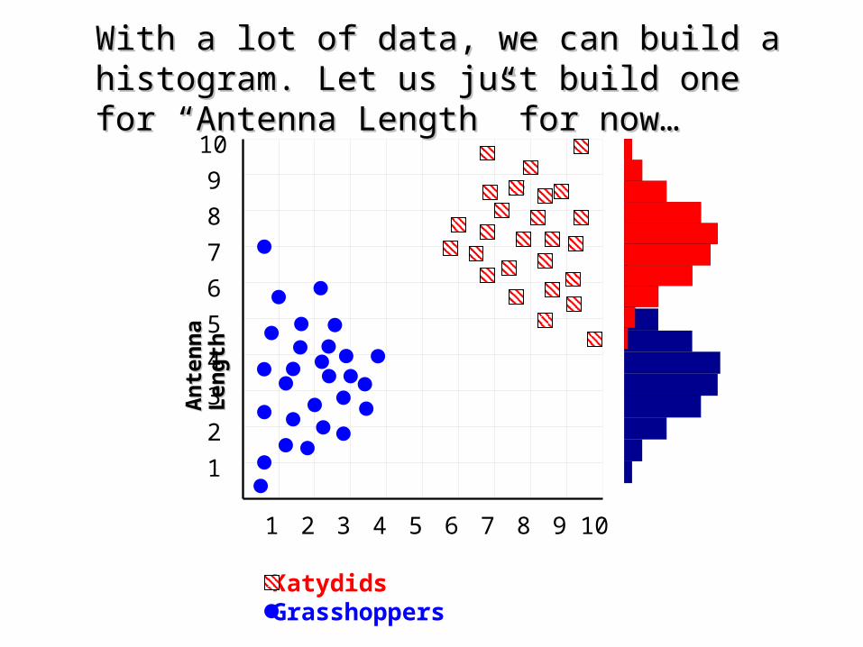
KatydidsGrasshoppers
With a lot of data, we can build a histogram. Let us With a lot of data, we can build a histogram. Let us just build one for “Antenna Length” for now…just build one for “Antenna Length” for now…
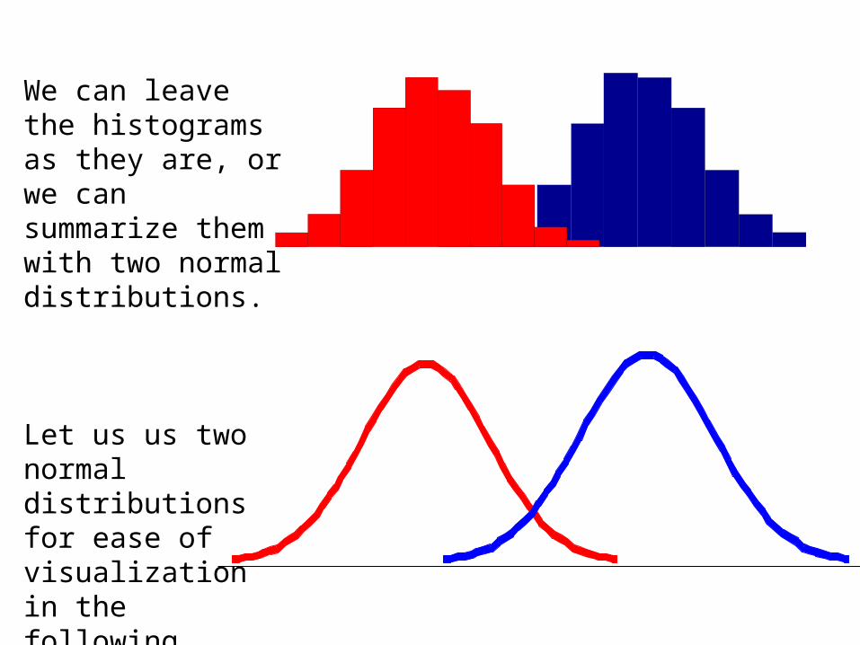
We can leave the histograms as they are, or we can summarize them with two normal distributions.
Let us us two normal distributions for ease of visualization in the following slides…

p(cj | d) = probability of class cj, given that we have observed dp(cj | d) = probability of class cj, given that we have observed d
3
Antennae length is 3
• We want to classify an insect we have found. Its antennae are 3 units long. How can we classify it?
• We can just ask ourselves, give the distributions of antennae lengths we have seen, is it more probable that our insect is a Grasshopper or a Katydid.• There is a formal way to discuss the most probable classification…

10
2
P(Grasshopper | 3 ) = 10 / (10 + 2) = 0.833
P(Katydid | 3 ) = 2 / (10 + 2) = 0.166
3
Antennae length is 3
p(cj | d) = probability of class cj, given that we have observed dp(cj | d) = probability of class cj, given that we have observed d
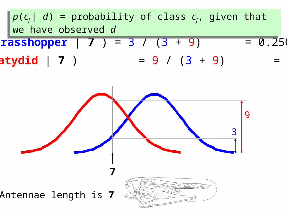
9
3
P(Grasshopper | 7 ) = 3 / (3 + 9) = 0.250
P(Katydid | 7 ) = 9 / (3 + 9) = 0.750
7
Antennae length is 7
p(cj | d) = probability of class cj, given that we have observed dp(cj | d) = probability of class cj, given that we have observed d
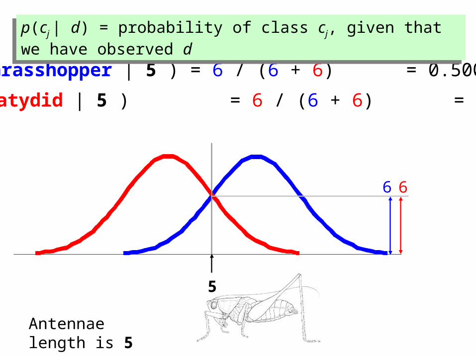
66
P(Grasshopper | 5 ) = 6 / (6 + 6) = 0.500
P(Katydid | 5 ) = 6 / (6 + 6) = 0.500
5
Antennae length is 5
p(cj | d) = probability of class cj, given that we have observed dp(cj | d) = probability of class cj, given that we have observed d
Bayes ClassifiersBayes Classifiers
That was a visual intuition for a simple case of the Bayes classifier, also called:
• Idiot Bayes • Naïve Bayes• Simple Bayes
We are about to see some of the mathematical formalisms, and more examples, but keep in mind the basic idea.
Find out the probability of the previously unseen instance previously unseen instance belonging to each class, then simply pick the most probable class.
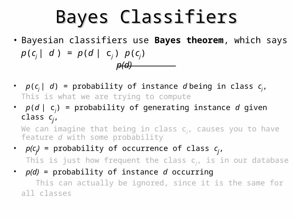
Bayes ClassifiersBayes Classifiers• Bayesian classifiers use Bayes theorem, which says
p(cj | d ) = p(d | cj ) p(cj) p(d)
• p(cj | d) = probability of instance d being in class cj, This is what we are trying to compute
• p(d | cj) = probability of generating instance d given class cj,
We can imagine that being in class cj, causes you to have feature d with some probability
• p(cj) = probability of occurrence of class cj,
This is just how frequent the class cj, is in our database
• p(d) = probability of instance d occurring
This can actually be ignored, since it is the same for all classes

Assume that we have two classes
c1 = malemale, and c2 = femalefemale.
We have a person whose sex we do not know, say “drew” or d.
Classifying drew as male or female is equivalent to asking is it more probable that drew is malemale or femalefemale, I.e which is greater p(malemale | drew) or p(femalefemale | drew)
p(malemale | drew) = p(drew | malemale ) p(malemale)
p(drew)
(Note: “Drew can be a male or female name”)
What is the probability of being called “drew” given that you are a male?
What is the probability of being a male?
What is the probability of being named “drew”? (actually irrelevant, since it is that same for all classes)
Drew Carey
Drew Barrymore
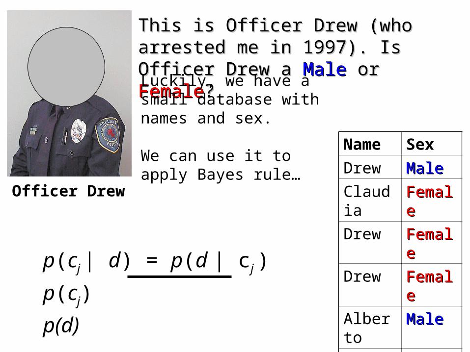
p(cj | d) = p(d | cj ) p(cj)
p(d)
Officer Drew
Name Sex
Drew MaleMale
Claudia FemaleFemale
Drew FemaleFemale
Drew FemaleFemale
Alberto MaleMale
Karin FemaleFemale
Nina FemaleFemale
Sergio MaleMale
This is Officer Drew (who arrested me in This is Officer Drew (who arrested me in 1997). Is Officer Drew a 1997). Is Officer Drew a MaleMale or or FemaleFemale??
Luckily, we have a small database with names and sex.
We can use it to apply Bayes rule…
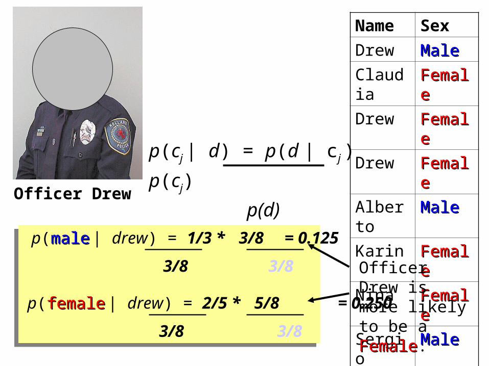
p(malemale | drew) = 1/3 * 3/8 = 0.125
3/8 3/8
p(femalefemale | drew) = 2/5 * 5/8 = 0.250
3/8 3/8
Officer Drew
p(cj | d) = p(d | cj ) p(cj)
p(d)
Name Sex
Drew MaleMale
Claudia FemaleFemale
Drew FemaleFemale
Drew FemaleFemale
Alberto MaleMale
Karin FemaleFemale
Nina FemaleFemale
Sergio MaleMale
Officer Drew is more likely to be a FemaleFemale.

Officer Drew IS a female!Officer Drew IS a female!
Officer Drew
p(malemale | drew) = 1/3 * 3/8 = 0.125
3/8 3/8
p(femalefemale | drew) = 2/5 * 5/8 = 0.250
3/8 3/8

Name Over 170CM Eye Hair length Sex
Drew No Blue Short MaleMale
Claudia Yes Brown Long FemaleFemale
Drew No Blue Long FemaleFemale
Drew No Blue Long FemaleFemale
Alberto Yes Brown Short MaleMale
Karin No Blue Long FemaleFemale
Nina Yes Brown Short FemaleFemale
Sergio Yes Blue Long MaleMale
p(cj | d) = p(d | cj ) p(cj)
p(d)
So far we have only considered Bayes Classification when we have one attribute (the “antennae length”, or the “name”). But we may have many features.How do we use all the features?
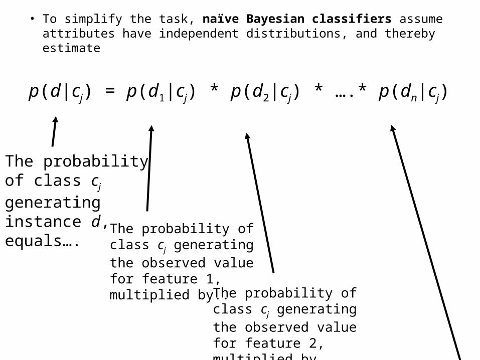
• To simplify the task, naïve Bayesian classifiers assume attributes have independent distributions, and thereby estimate
p(d|cj) = p(d1|cj) * p(d2|cj) * ….* p(dn|cj)
The probability of class cj generating instance d, equals….
The probability of class cj generating the observed value for feature 1, multiplied by..
The probability of class cj generating the observed value for feature 2, multiplied by..
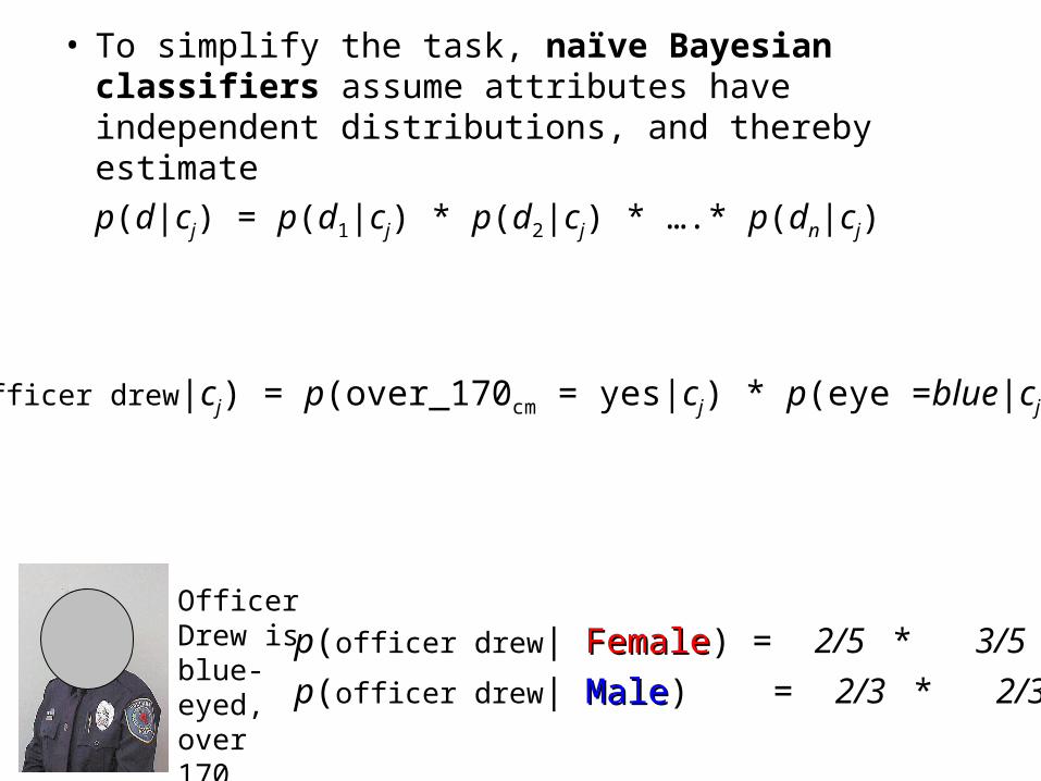
• To simplify the task, naïve Bayesian classifiers assume attributes have independent distributions, and thereby estimate
p(d|cj) = p(d1|cj) * p(d2|cj) * ….* p(dn|cj)
p(officer drew|cj) = p(over_170cm = yes|cj) * p(eye =blue|cj) * ….
Officer Drew is blue-eyed, over 170cm tall, and has long hair
p(officer drew| FemaleFemale) = 2/5 * 3/5 * ….
p(officer drew| MaleMale) = 2/3 * 2/3 * ….

p(d1|cj) p(d2|cj) p(dn|cj)
cjThe Naive Bayes classifiers is often represented as this type of graph…
Note the direction of the arrows, which state that each class causes certain features, with a certain probability
…
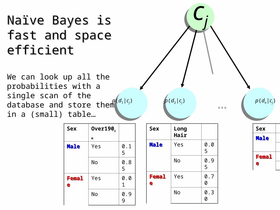
Naïve Bayes is fast and Naïve Bayes is fast and space efficientspace efficient
We can look up all the probabilities with a single scan of the database and store them in a (small) table…
Sex Over190cm
MaleMale Yes 0.15
No 0.85
FemaleFemale Yes 0.01
No 0.99
cj
…p(d1|cj) p(d2|cj) p(dn|cj)
Sex Long Hair
MaleMale Yes 0.05
No 0.95
FemaleFemale Yes 0.70
No 0.30
Sex
MaleMale
FemaleFemale
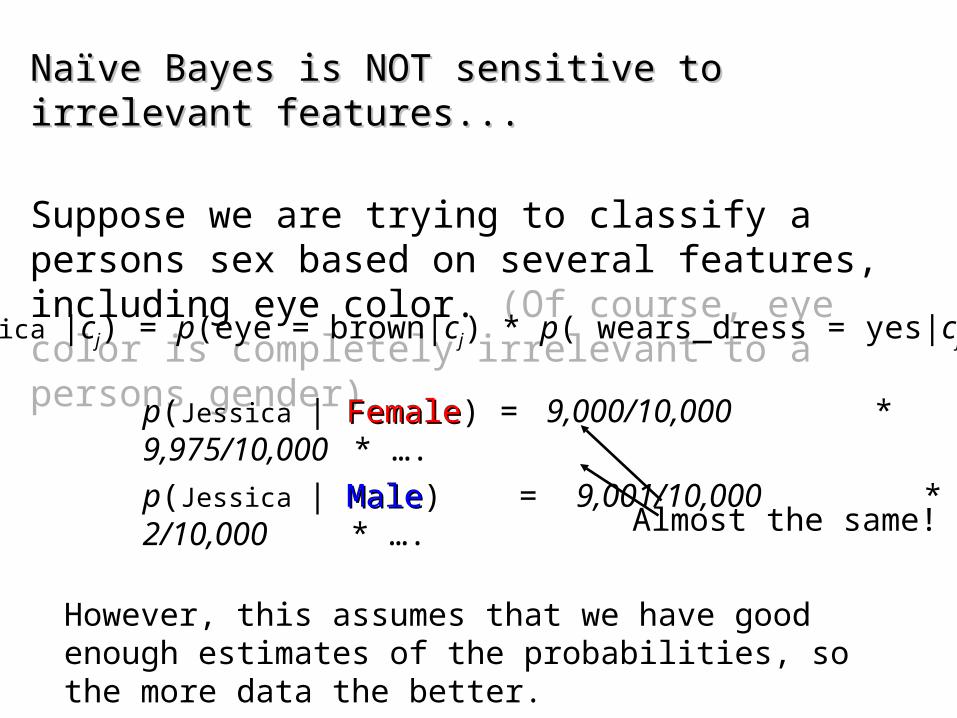
Naïve Bayes is NOT sensitive to irrelevant features...Naïve Bayes is NOT sensitive to irrelevant features...
Suppose we are trying to classify a persons sex based on several features, including eye color. (Of course, eye color is completely irrelevant to a persons gender)
p(Jessica | FemaleFemale) = 9,000/10,000 * 9,975/10,000 * ….
p(Jessica | MaleMale) = 9,001/10,000 * 2/10,000 * ….
p(Jessica |cj) = p(eye = brown|cj) * p( wears_dress = yes|cj) * ….
However, this assumes that we have good enough estimates of the probabilities, so the more data the better.
Almost the same!
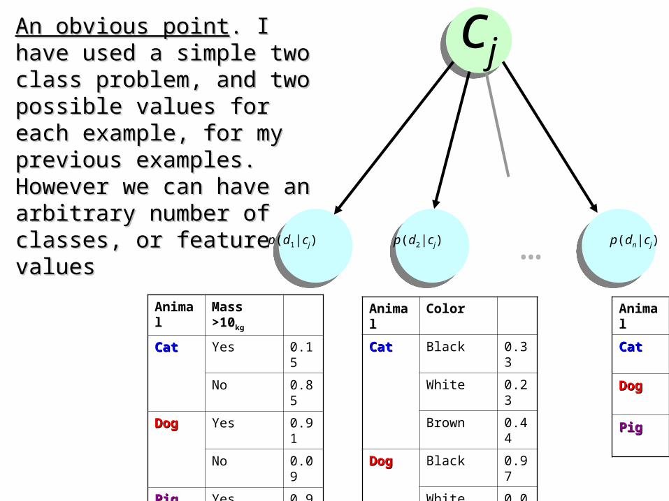
An obvious pointAn obvious point. I have used a . I have used a simple two class problem, and simple two class problem, and two possible values for each two possible values for each example, for my previous example, for my previous examples. However we can have examples. However we can have an arbitrary number of classes, or an arbitrary number of classes, or feature valuesfeature values
Animal Mass >10kg
CatCat Yes 0.15
No 0.85
DogDog Yes 0.91
No 0.09
PigPig Yes 0.99
No 0.01
cj
…p(d1|cj) p(d2|cj) p(dn|cj)
Animal
CatCat
DogDog
PigPig
Animal Color
CatCat Black 0.33
White 0.23
Brown 0.44
DogDog Black 0.97
White 0.03
Brown 0.90
PigPig Black 0.04
White 0.01
Brown 0.95
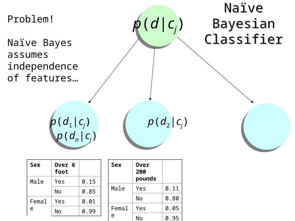
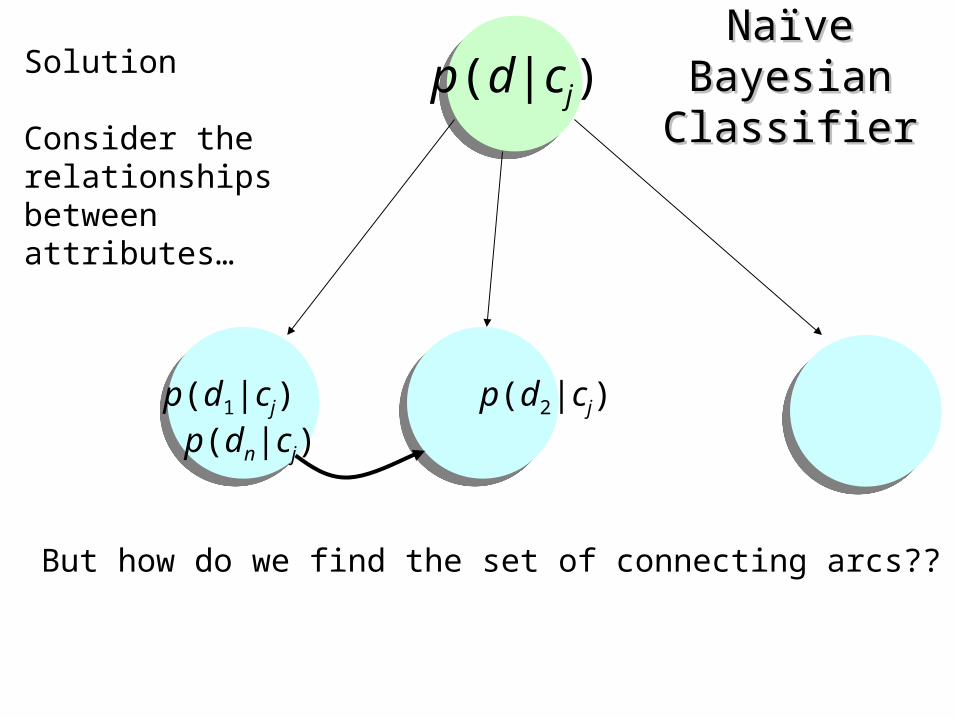
Naïve Bayesian Naïve Bayesian ClassifierClassifier
p(d1|cj) p(d2|cj) p(dn|cj)
p(d|cj)Problem!
Naïve Bayes assumes independence of features…
Sex Over 6 foot
Male Yes 0.15
No 0.85
Female Yes 0.01
No 0.99
Sex Over 200 pounds
Male Yes 0.11
No 0.80
Female Yes 0.05
No 0.95

Naïve Bayesian Naïve Bayesian ClassifierClassifier
p(d1|cj) p(d2|cj) p(dn|cj)
p(d|cj)Solution
Consider the relationships between attributes…
Sex Over 6 foot
Male Yes 0.15
No 0.85
Female Yes 0.01
No 0.99
Sex Over 200 pounds
Male Yes and Over 6 foot 0.11
No and Over 6 foot 0.59
Yes and NOT Over 6 foot 0.05
No and NOT Over 6 foot 0.35
Female Yes and Over 6 foot 0.01
Naïve Bayesian Naïve Bayesian ClassifierClassifier
p(d1|cj) p(d2|cj) p(dn|cj)
p(d|cj)Solution
Consider the relationships between attributes…
But how do we find the set of connecting arcs??

10
1 2 3 4 5 6 7 8 9 10
1
2
3
4
5
6
7
8
9
The Naïve Bayesian ClassifierThe Naïve Bayesian Classifierhas a quadratic decision boundaryhas a quadratic decision boundary

Dear SIR,
I am Mr. John Coleman and my sister is Miss Rose Colemen, we are the children of late Chief Paul Colemen from Sierra Leone. I am writing you in absolute confidence primarily to seek your assistance to transfer our cash of twenty one Million Dollars ($21,000.000.00) now in the custody of a private Security trust firm in Europe the money is in trunk boxes deposited and declared as family valuables by my late father as a matter of fact the company does not know the content as money, although my father made them to under stand that the boxes belongs to his foreign partner.…
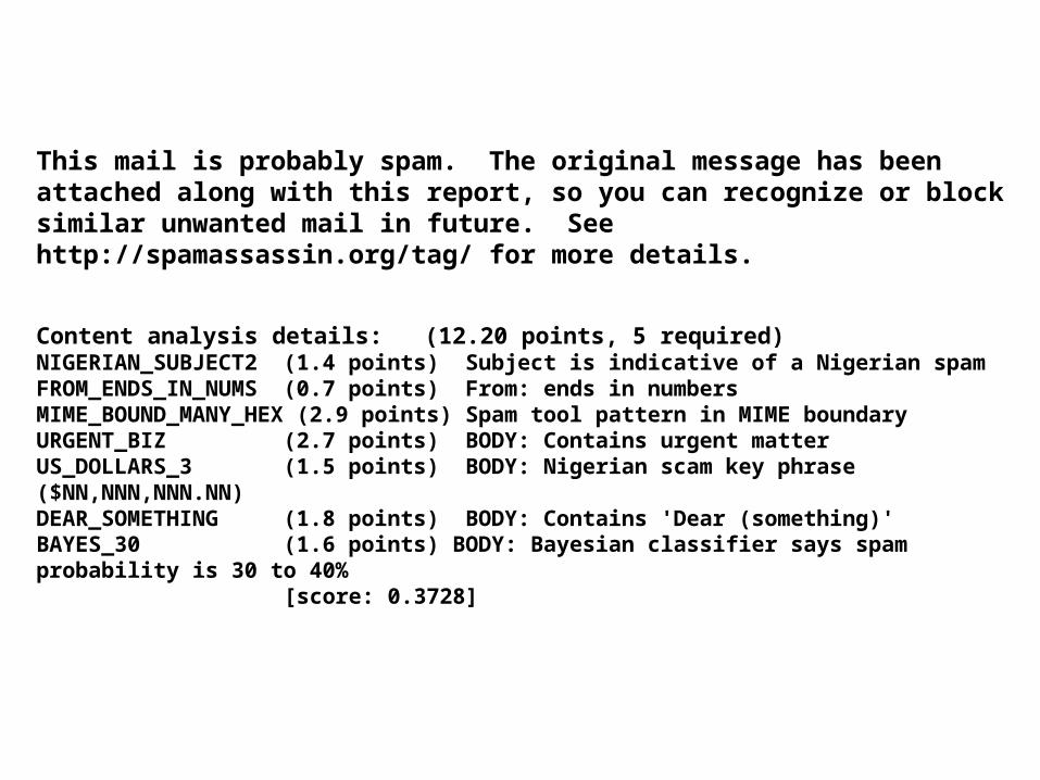
This mail is probably spam. The original message has been attached along with this report, so you can recognize or block similar unwanted mail in future. See http://spamassassin.org/tag/ for more details.
Content analysis details: (12.20 points, 5 required)NIGERIAN_SUBJECT2 (1.4 points) Subject is indicative of a Nigerian spamFROM_ENDS_IN_NUMS (0.7 points) From: ends in numbersMIME_BOUND_MANY_HEX (2.9 points) Spam tool pattern in MIME boundaryURGENT_BIZ (2.7 points) BODY: Contains urgent matterUS_DOLLARS_3 (1.5 points) BODY: Nigerian scam key phrase ($NN,NNN,NNN.NN)DEAR_SOMETHING (1.8 points) BODY: Contains 'Dear (something)'BAYES_30 (1.6 points) BODY: Bayesian classifier says spam probability is 30 to 40% [score: 0.3728]
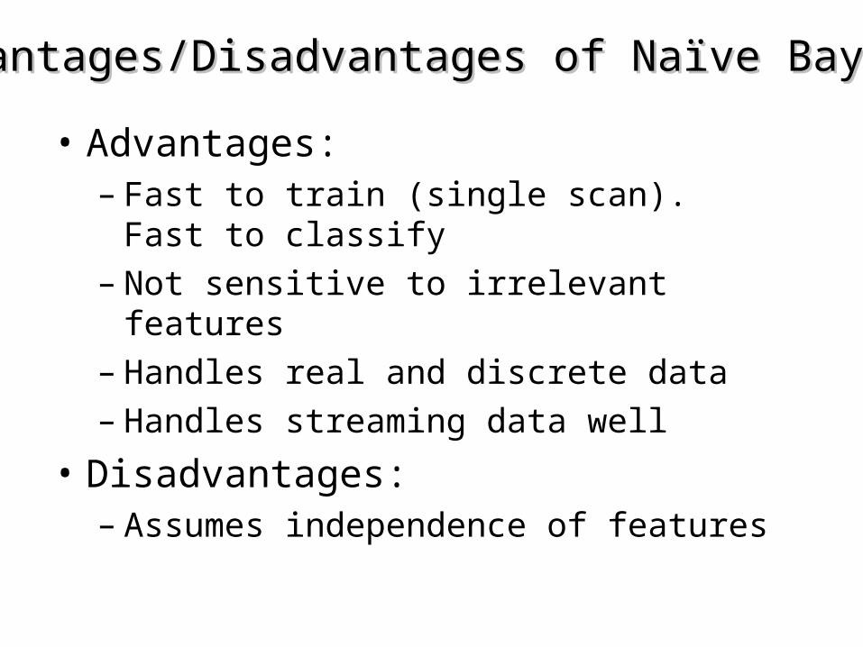
• Advantages:– Fast to train (single scan). Fast to classify – Not sensitive to irrelevant features– Handles real and discrete data– Handles streaming data well
• Disadvantages:– Assumes independence of features
Advantages/Disadvantages of Naïve BayesAdvantages/Disadvantages of Naïve Bayes

Summary of ClassificationSummary of Classification
We have seen 4 major classification techniques:• Simple linear classifier, Nearest neighbor, Decision tree.
There are other techniques:• Neural Networks, Support Vector Machines, Genetic algorithms..
In general, there is no one best classifier for all problems. You have to consider what you hope to achieve, and the data itself…
Let us now move on to the other classic problem of data mining and machine learning, Clustering…
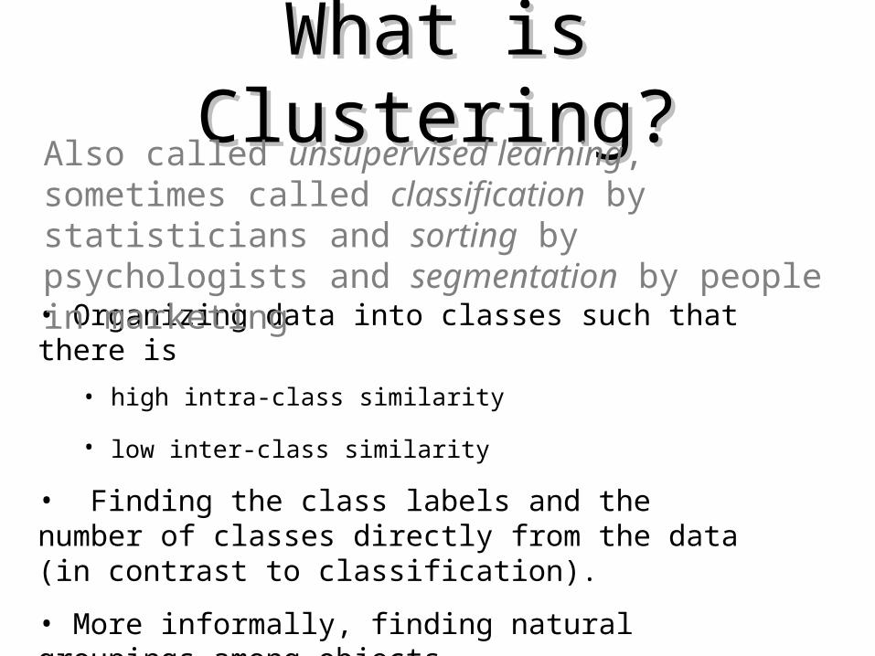
• Organizing data into classes such that there is
• high intra-class similarity
• low inter-class similarity
• Finding the class labels and the number of classes directly from the data (in contrast to classification).
• More informally, finding natural groupings among objects.
What is Clustering?What is Clustering?Also called unsupervised learning, sometimes called classification by statisticians and sorting by psychologists and segmentation by people in marketing

What is a natural grouping among these objects?What is a natural grouping among these objects?

School Employees Simpson's Family Males Females
Clustering is subjectiveClustering is subjective
What is a natural grouping among these objects?What is a natural grouping among these objects?

What is Similarity?What is Similarity?The quality or state of being similar; likeness; resemblance; as, a similarity of features.
Similarity is hard to define, but… “We know it when we see it”
The real meaning of similarity is a philosophical question. We will take a more pragmatic approach.
Webster's Dictionary
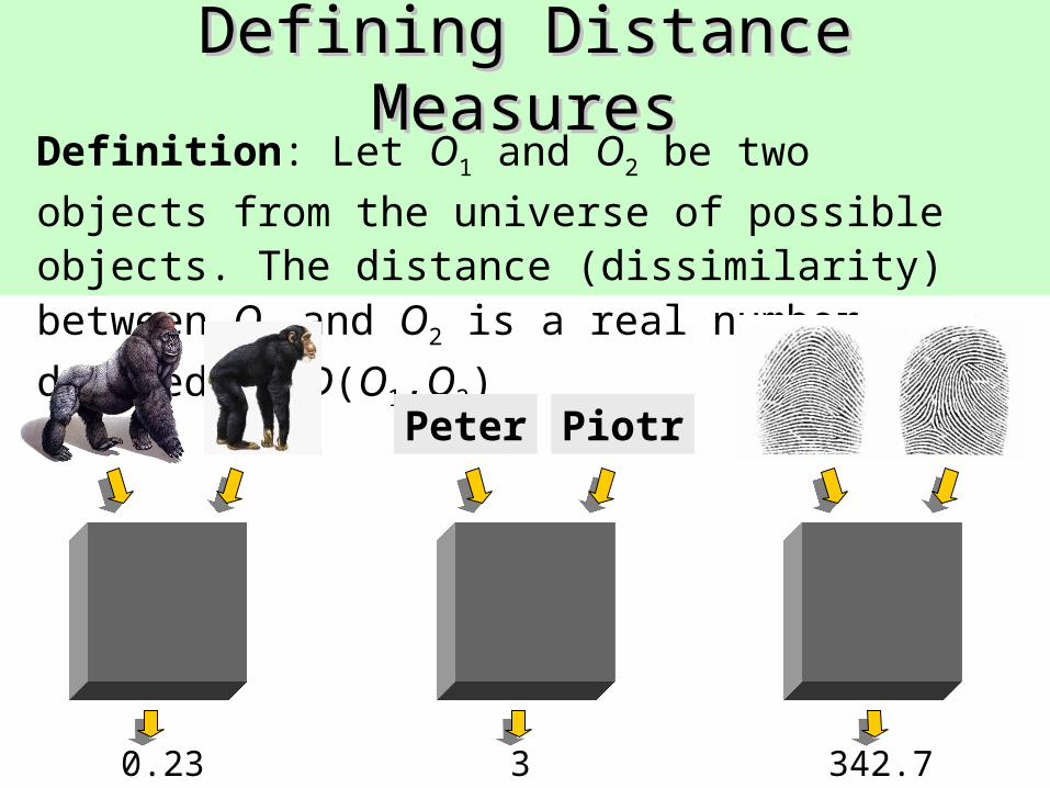
Defining Distance MeasuresDefining Distance MeasuresDefinition: Let O1 and O2 be two objects from the universe
of possible objects. The distance (dissimilarity) between O1 and O2 is a real number denoted by D(O1,O2)
0.23 3 342.7
Peter Piotr
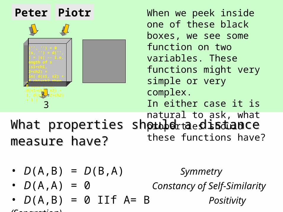
What properties should a distance measure have?What properties should a distance measure have?
• D(A,B) = D(B,A) Symmetry
• D(A,A) = 0 Constancy of Self-Similarity
• D(A,B) = 0 IIf A= B Positivity (Separation)
• D(A,B) D(A,C) + D(B,C) Triangular Inequality
Peter Piotr
3
d('', '') = 0 d(s, '') = d('', s) = |s| -- i.e. length of s d(s1+ch1, s2+ch2) = min( d(s1, s2) + if ch1=ch2 then 0 else 1 fi, d(s1+ch1, s2) + 1, d(s1, s2+ch2) + 1 )
When we peek inside one of these black boxes, we see some function on two variables. These functions might very simple or very complex. In either case it is natural to ask, what properties should these functions have?
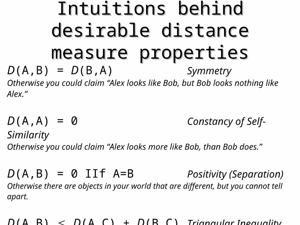
Intuitions behind desirable Intuitions behind desirable distance measure propertiesdistance measure properties
D(A,B) = D(B,A) Symmetry Otherwise you could claim “Alex looks like Bob, but Bob looks nothing like Alex.”
D(A,A) = 0 Constancy of Self-SimilarityOtherwise you could claim “Alex looks more like Bob, than Bob does.”
D(A,B) = 0 IIf A=B Positivity (Separation)Otherwise there are objects in your world that are different, but you cannot tell apart.
D(A,B) D(A,C) + D(B,C) Triangular Inequality Otherwise you could claim “Alex is very like Bob, and Alex is very like Carl, but Bob is very unlike Carl.”
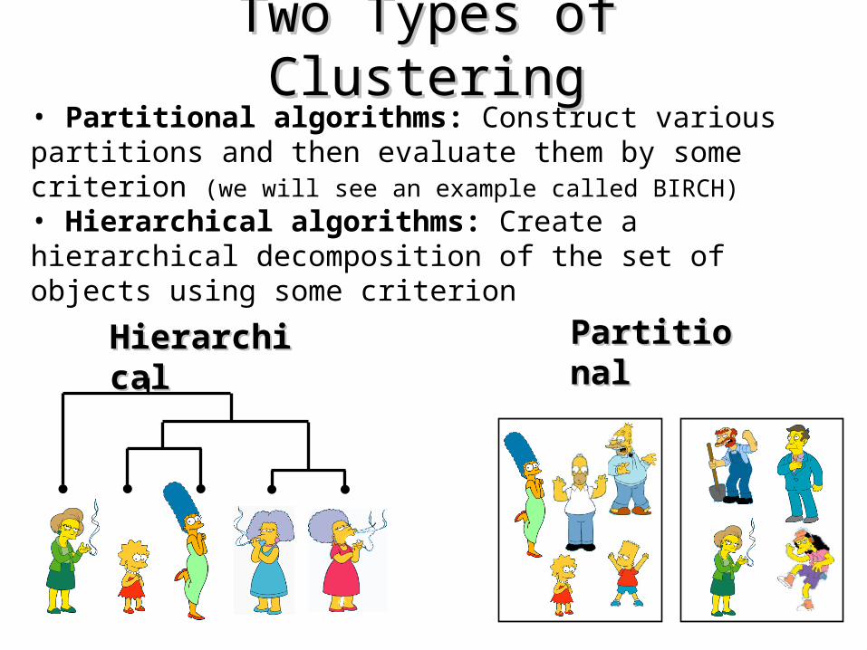
Two Types of ClusteringTwo Types of Clustering
HierarchicalHierarchical
• Partitional algorithms: Construct various partitions and then evaluate them by some criterion (we will see an example called BIRCH)• Hierarchical algorithms: Create a hierarchical decomposition of the set of objects using some criterion
PartitionalPartitional
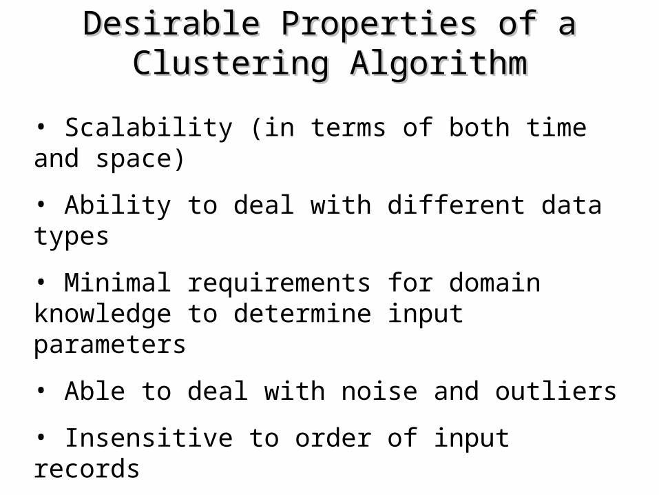
Desirable Properties of a Clustering AlgorithmDesirable Properties of a Clustering Algorithm
• Scalability (in terms of both time and space)
• Ability to deal with different data types
• Minimal requirements for domain knowledge to determine input parameters
• Able to deal with noise and outliers
• Insensitive to order of input records
• Incorporation of user-specified constraints
• Interpretability and usability

A Useful Tool for Summarizing Similarity MeasurementsA Useful Tool for Summarizing Similarity Measurements In order to better appreciate and evaluate the examples given in the early part of this talk, we will now introduce the dendrogram.
Root
Internal Branch
Terminal Branch
Leaf
Internal Node
Root
Internal Branch
Terminal Branch
Leaf
Internal Node
The similarity between two objects in a dendrogram is represented as the height of the lowest internal node they share.

(Bovine:0.69395, (Spider Monkey 0.390, (Gibbon:0.36079,(Orang:0.33636,(Gorilla:0.17147,(Chimp:0.19268, Human:0.11927):0.08386):0.06124):0.15057):0.54939);
There is only one dataset that can be There is only one dataset that can be perfectly clustered using a hierarchy… perfectly clustered using a hierarchy…
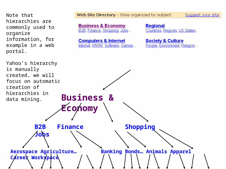
Business & Economy
B2B Finance Shopping Jobs
Aerospace Agriculture… Banking Bonds… Animals Apparel Career Workspace
Note that hierarchies are commonly used to organize information, for example in a web portal.
Yahoo’s hierarchy is manually created, we will focus on automatic creation of hierarchies in data mining.

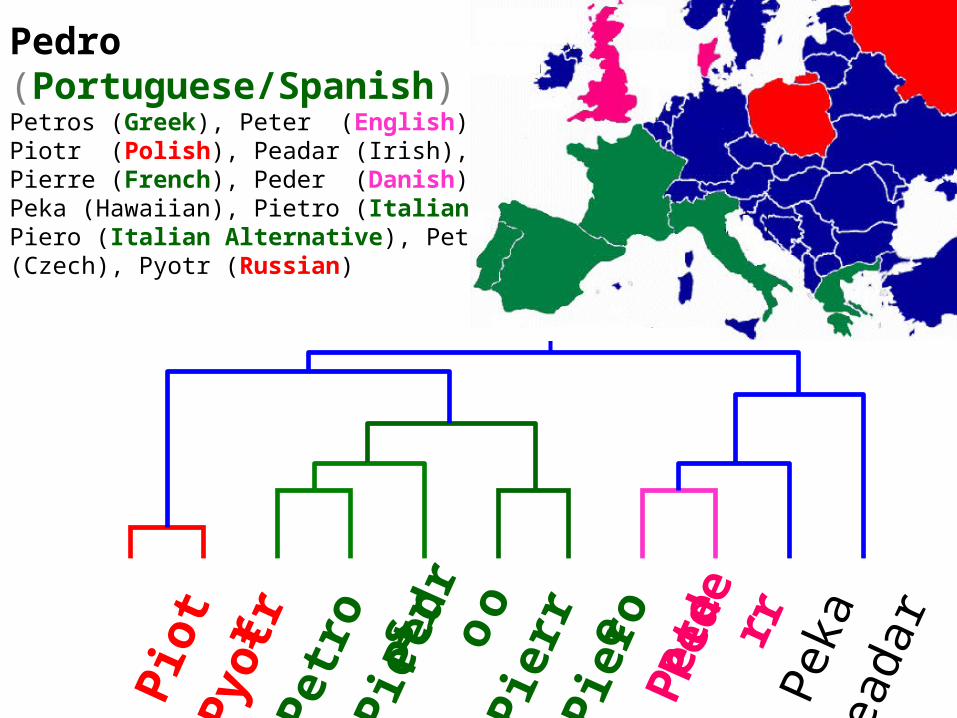
Pedro (Portuguese)Petros (Greek), Peter (English), Piotr (Polish), Peadar (Irish), Pierre (French), Peder (Danish), Peka (Hawaiian), Pietro (Italian), Piero (Italian Alternative), Petr (Czech), Pyotr (Russian)
Cristovao (Portuguese)Christoph (German), Christophe (French), Cristobal (Spanish), Cristoforo (Italian), Kristoffer (Scandinavian), Krystof (Czech), Christopher (English)
Miguel (Portuguese)Michalis (Greek), Michael (English), Mick (Irish!)
A Demonstration of Hierarchical Clustering using String Edit Distance A Demonstration of Hierarchical Clustering using String Edit Distance P
iotr
Pyo
tr P
etro
s P
ietr
oPe
dro
Pie
rre
Pie
ro P
eter
Pede
r P
eka
Pea
dar
Mic
halis
Mic
hael
Mig
uel
Mic
kC
rist
ovao
Chr
isto
pher
Chr
isto
phe
Chr
isto
phC
risd
ean
Cri
stob
alC
rist
ofor
oK
rist
offe
rK
ryst
of
Pio
tr P
yotr
Pet
ros
Pie
tro
Ped
ro P
ierr
e P
iero
Pet
erP
eder
Pek
a P
eada
r
Pedro (Portuguese/Spanish)Petros (Greek), Peter (English), Piotr (Polish), Peadar (Irish), Pierre (French), Peder (Danish), Peka (Hawaiian), Pietro (Italian), Piero (Italian Alternative), Petr (Czech), Pyotr (Russian)
ANGUILLAAUSTRALIA
St. Helena & Dependencies
South Georgia &South Sandwich Islands U.K.
Serbia & Montenegro(Yugoslavia) FRANCE NIGER INDIA IRELAND BRAZIL
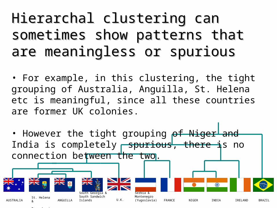
Hierarchal clustering can sometimes show Hierarchal clustering can sometimes show patterns that are meaningless or spuriouspatterns that are meaningless or spurious
• For example, in this clustering, the tight grouping of Australia, Anguilla, St. Helena etc is meaningful, since all these countries are former UK colonies.
• However the tight grouping of Niger and India is completely spurious, there is no connection between the two.

ANGUILLAAUSTRALIA
St. Helena & Dependencies
South Georgia &South Sandwich Islands U.K.
Serbia & Montenegro(Yugoslavia) FRANCE NIGER INDIA IRELAND BRAZIL
• The flag of Niger is orange over white over green, with an orange disc on the central white stripe, symbolizing the sun. The orange stands the Sahara desert, which borders Niger to the north. Green stands for the grassy plains of the south and west and for the River Niger which sustains them. It also stands for fraternity and hope. White generally symbolizes purity and hope.
• The Indian flag is a horizontal tricolor in equal proportion of deep saffron on the top, white in the middle and dark green at the bottom. In the center of the white band, there is a wheel in navy blue to indicate the Dharma Chakra, the wheel of law in the Sarnath Lion Capital. This center symbol or the 'CHAKRA' is a symbol dating back to 2nd century BC. The saffron stands for courage and sacrifice; the white, for purity and truth; the green for growth and auspiciousness.
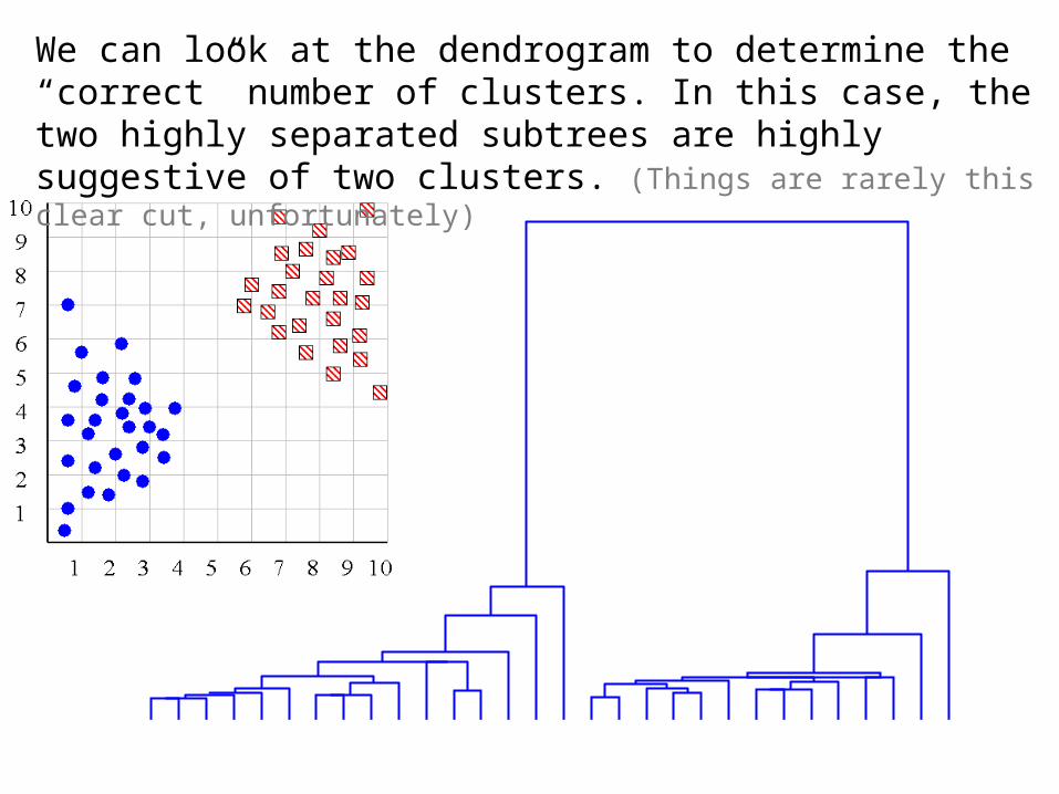
We can look at the dendrogram to determine the “correct” number of clusters. In this case, the two highly separated subtrees are highly suggestive of two clusters. (Things are rarely this clear cut, unfortunately)
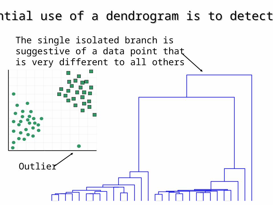
Outlier
One potential use of a dendrogram is to detect outliersOne potential use of a dendrogram is to detect outliers
The single isolated branch is suggestive of a data point that is very different to all others

(How-to) Hierarchical ClusteringThe number of dendrograms with n
leafs = (2n -3)!/[(2(n -2)) (n -2)!]
Number Number of Possibleof Leafs Dendrograms 2 13 34 155 105... …10 34,459,425
Since we cannot test all possible trees we will have to heuristic search of all possible trees. We could do this..
Bottom-Up (agglomerative): Starting with each item in its own cluster, find the best pair to merge into a new cluster. Repeat until all clusters are fused together.
Top-Down (divisive): Starting with all the data in a single cluster, consider every possible way to divide the cluster into two. Choose the best division and recursively operate on both sides.

0 8 8 7 7
0 2 4 4
0 3 3
0 1
0
D( , ) = 8
D( , ) = 1
We begin with a distance matrix which contains the distances between every pair of objects in our database.
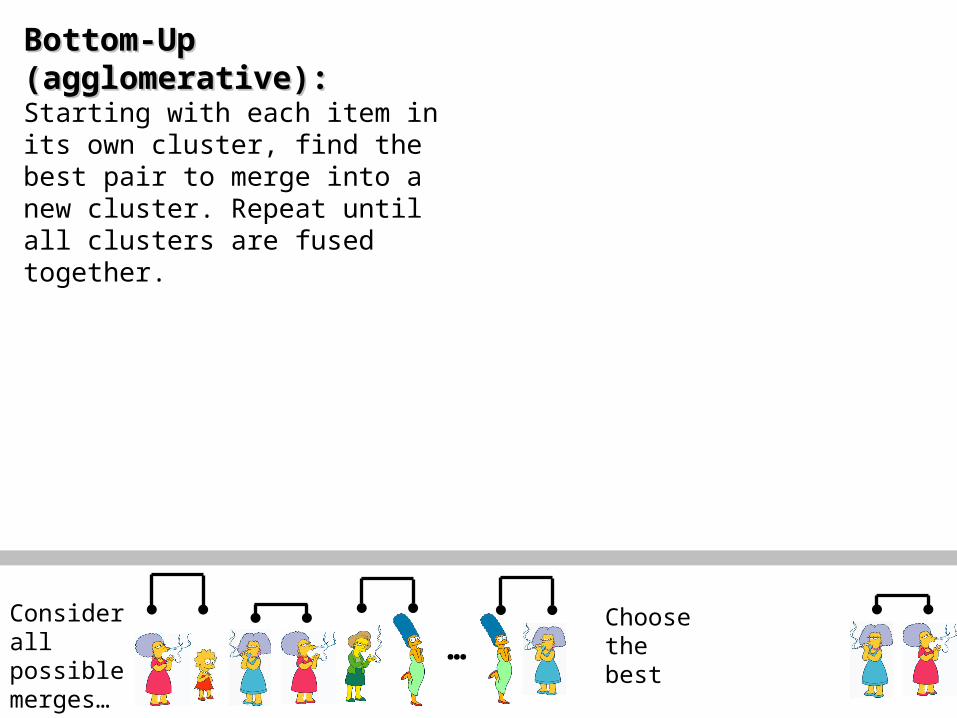
Bottom-Up (Bottom-Up (agglomerativeagglomerative):): Starting with each item in its own cluster, find the best pair to merge into a new cluster. Repeat until all clusters are fused together.
…Consider all possible merges…
Choose the best
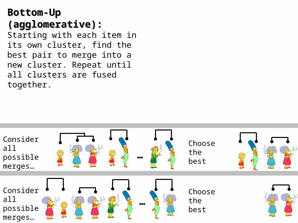
Bottom-Up (Bottom-Up (agglomerativeagglomerative):): Starting with each item in its own cluster, find the best pair to merge into a new cluster. Repeat until all clusters are fused together.
…Consider all possible merges…
Choose the best
Consider all possible merges… …
Choose the best
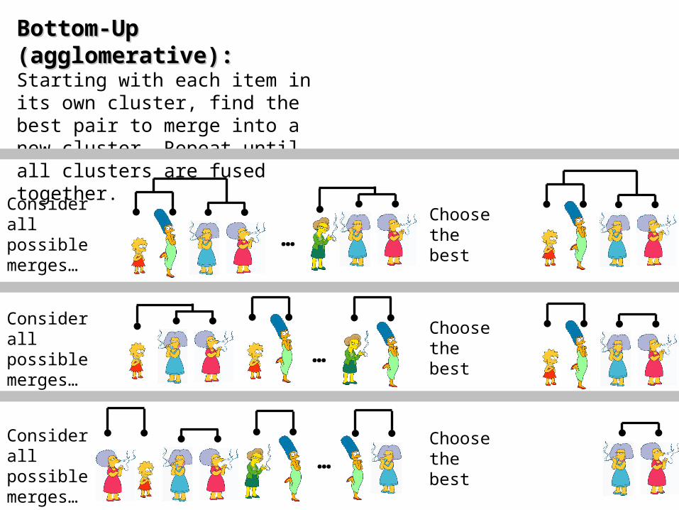
Bottom-Up (Bottom-Up (agglomerativeagglomerative):): Starting with each item in its own cluster, find the best pair to merge into a new cluster. Repeat until all clusters are fused together.
…Consider all possible merges…
Choose the best
Consider all possible merges… …
Choose the best
Consider all possible merges…
Choose the best…

We know how to measure the distance between two We know how to measure the distance between two objects, but defining the distance between an object objects, but defining the distance between an object and a cluster, or defining the distance between two and a cluster, or defining the distance between two clusters is non obvious. clusters is non obvious.
• Single linkage (nearest neighbor):Single linkage (nearest neighbor): In this method the distance between two clusters is determined by the distance of the two closest objects (nearest neighbors) in the different clusters.• Complete linkage (furthest neighbor):Complete linkage (furthest neighbor): In this method, the distances between clusters are determined by the greatest distance between any
two objects in the different clusters (i.e., by the "furthest neighbors"). • Group average linkageGroup average linkage: In this method, the distance between two clusters is calculated as the average distance between all pairs of objects in the
two different clusters.• Wards LinkageWards Linkage: In this method, we try to minimize the variance of the merged clusters

29 2 6 11 9 17 10 13 24 25 26 20 22 30 27 1 3 8 4 12 5 14 23 15 16 18 19 21 28 7
1
2
3
4
5
6
7
Average linkage 5 14 23 7 4 12 19 21 24 15 16 18 1 3 8 9 29 2 10 11 20 28 17 26 27 25 6 13 22 30
0
5
10
15
20
25
Wards linkage
Single linkage
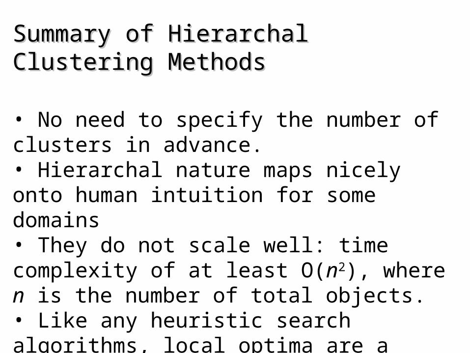
Summary of Hierarchal Clustering MethodsSummary of Hierarchal Clustering Methods
• No need to specify the number of clusters in advance. • Hierarchal nature maps nicely onto human intuition for some domains• They do not scale well: time complexity of at least O(n2), where n is the number of total objects.• Like any heuristic search algorithms, local optima are a problem.• Interpretation of results is (very) subjective.
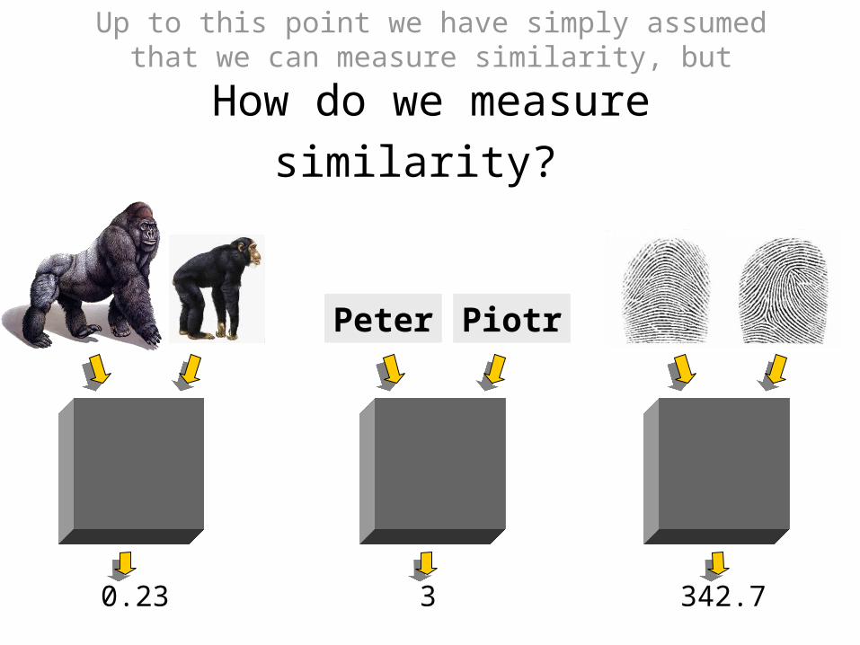
Up to this point we have simply assumed that we can measure similarity, but
How do we measure similarity?
0.23 3 342.7
Peter Piotr
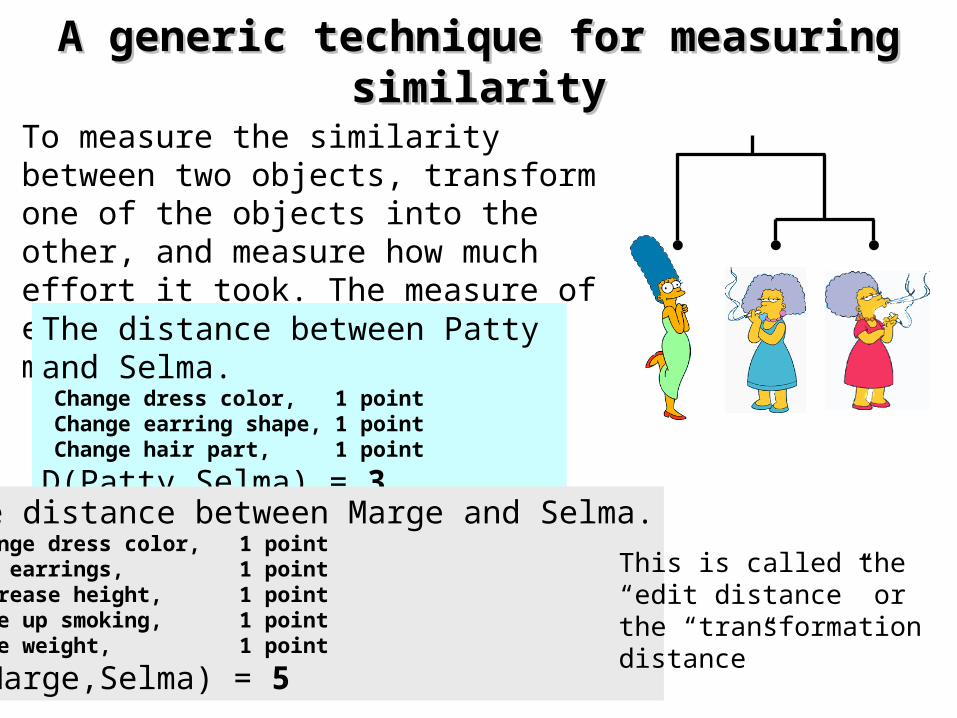
A generic technique for measuring similarityA generic technique for measuring similarity
To measure the similarity between two objects, transform one of the objects into the other, and measure how much effort it took. The measure of effort becomes the distance measure.
The distance between Patty and Selma. Change dress color, 1 point Change earring shape, 1 point Change hair part, 1 point
D(Patty,Selma) = 3
The distance between Marge and Selma. Change dress color, 1 point Add earrings, 1 point Decrease height, 1 point Take up smoking, 1 point Lose weight, 1 point
D(Marge,Selma) = 5
This is called the “edit distance” or the “transformation distance”

Peter
Piter
Pioter
Piotr
Substitution (i for e)
Insertion (o)
Deletion (e)
Edit Distance ExampleEdit Distance Example
It is possible to transform any string Q into string C, using only Substitution, Insertion and Deletion.Assume that each of these operators has a cost associated with it.
The similarity between two strings can be defined as the cost of the cheapest transformation from Q to C. Note that for now we have ignored the issue of how we can find this cheapest
transformation
How similar are the names “Peter” and “Piotr”?Assume the following cost function
Substitution 1 UnitInsertion 1 UnitDeletion 1 Unit
D(Peter,Piotr) is 3
Pio
tr P
yotr
Pet
ros
Pie
tro
Pedr
o P
ierr
e P
iero
Pet
er

Partitional ClusteringPartitional Clustering• Nonhierarchical, each instance is placed in
exactly one of K nonoverlapping clusters.
• Since only one set of clusters is output, the user normally has to input the desired number of clusters K.
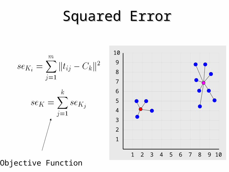
Squared ErrorSquared Error
10
1 2 3 4 5 6 7 8 9 10
1
2
3
4
5
6
7
8
9
Objective Function

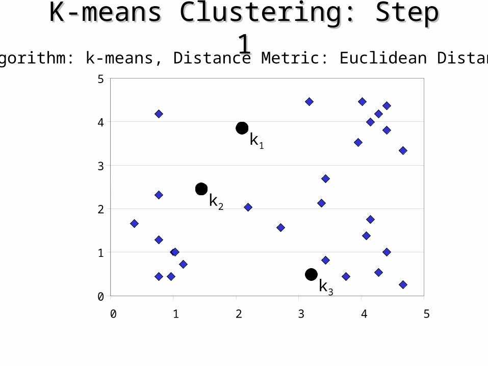
Algorithm k-means1. Decide on a value for k.
2. Initialize the k cluster centers (randomly, if necessary).
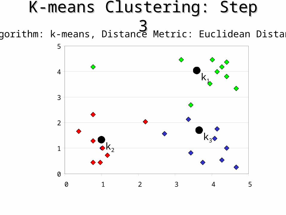
3. Decide the class memberships of the N objects by assigning them to the nearest cluster center.
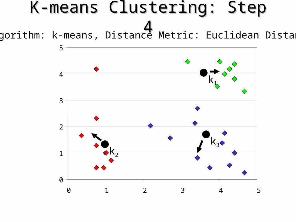
4. Re-estimate the k cluster centers, by assuming the memberships found above are correct.
5. If none of the N objects changed membership in the last iteration, exit. Otherwise goto 3.
0
1
2
3
4
5
0 1 2 3 4 5
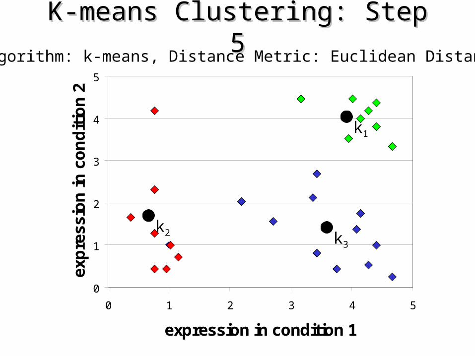
K-means Clustering: Step 1K-means Clustering: Step 1Algorithm: k-means, Distance Metric: Euclidean Distance
k1
k2
k3

0
1
2
3
4
5
0 1 2 3 4 5
K-means Clustering: Step 2K-means Clustering: Step 2Algorithm: k-means, Distance Metric: Euclidean Distance
k1
k2
k3
0
1
2
3
4
5
0 1 2 3 4 5
K-means Clustering: Step 3K-means Clustering: Step 3Algorithm: k-means, Distance Metric: Euclidean Distance
k1
k2
k3
0
1
2
3
4
5
0 1 2 3 4 5
K-means Clustering: Step 4K-means Clustering: Step 4Algorithm: k-means, Distance Metric: Euclidean Distance
k1
k2
k3
0
1
2
3
4
5
0 1 2 3 4 5
expression in condition 1
exp
ress
ion
in c
on
dit
ion
2
K-means Clustering: Step 5K-means Clustering: Step 5Algorithm: k-means, Distance Metric: Euclidean Distance
k1
k2 k3
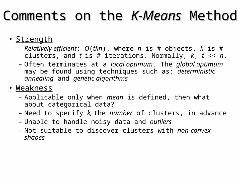
Comments on the Comments on the K-MeansK-Means Method Method
• Strength – Relatively efficient: O(tkn), where n is # objects, k is # clusters,
and t is # iterations. Normally, k, t << n.– Often terminates at a local optimum. The global optimum may
be found using techniques such as: deterministic annealing and genetic algorithms
• Weakness– Applicable only when mean is defined, then what about
categorical data?– Need to specify k, the number of clusters, in advance– Unable to handle noisy data and outliers– Not suitable to discover clusters with non-convex shapes

The K-Medoids Clustering Method
• Find representative objects, called medoids, in clusters
• PAM (Partitioning Around Medoids, 1987)– starts from an initial set of medoids and iteratively replaces
one of the medoids by one of the non-medoids if it improves the total distance of the resulting clustering
– PAM works effectively for small data sets, but does not scale well for large data sets
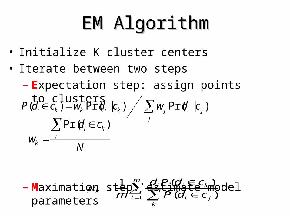
EM AlgorithmEM Algorithm
• Initialize K cluster centers• Iterate between two steps
– Expectation step: assign points to clusters
– Maximation step: estimate model parameters
j
jijkikki cdwcdwcdP ) |Pr() |Pr() (
m
ik
ji
kiik cdP
cdPd
m 1 ) (
) (1
N
cdw i
ki
k
) Pr(
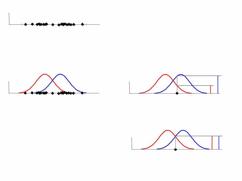
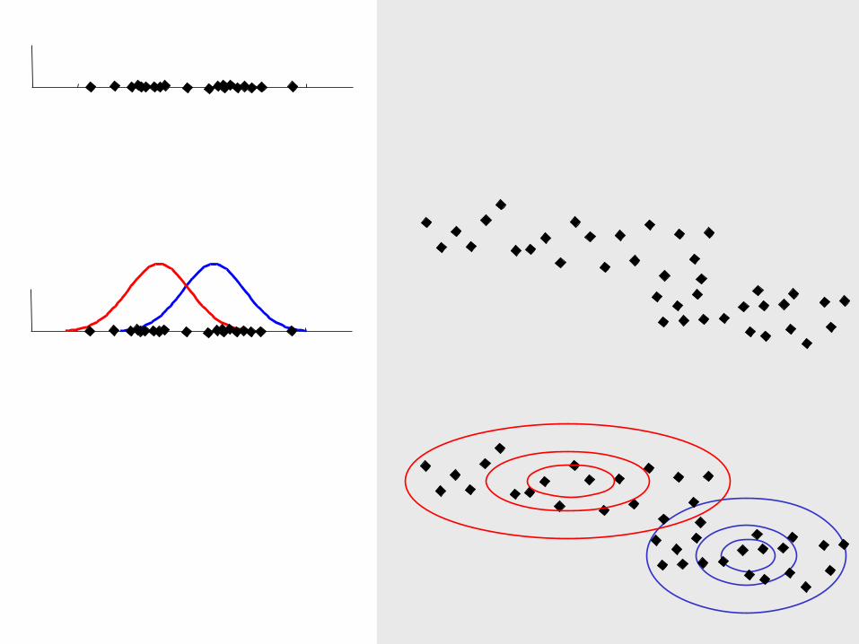

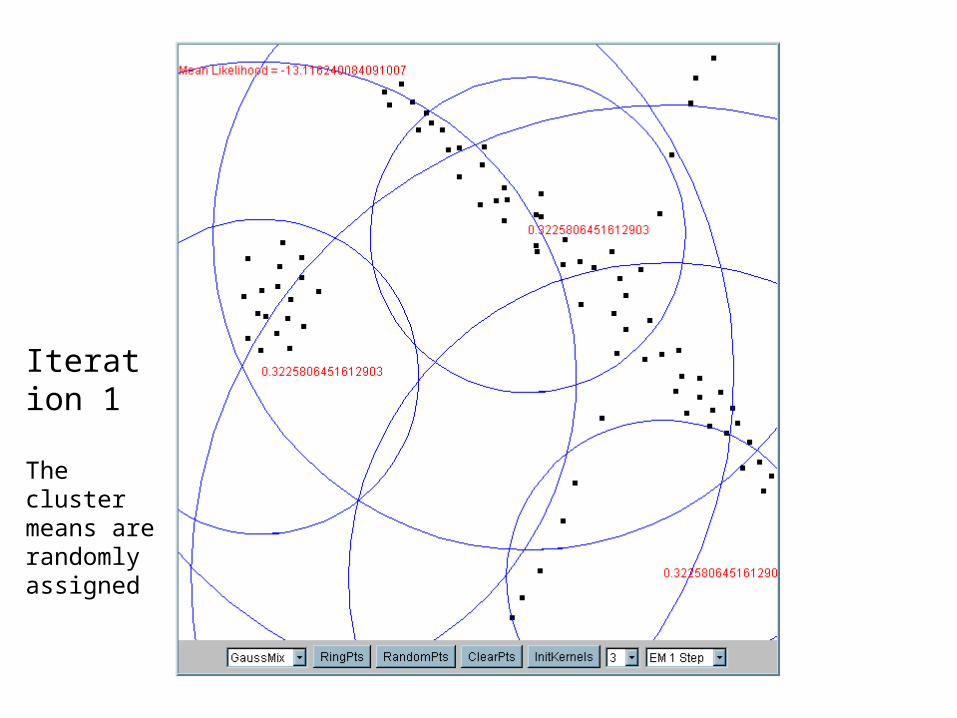
Iteration 1
The cluster means are randomly assigned
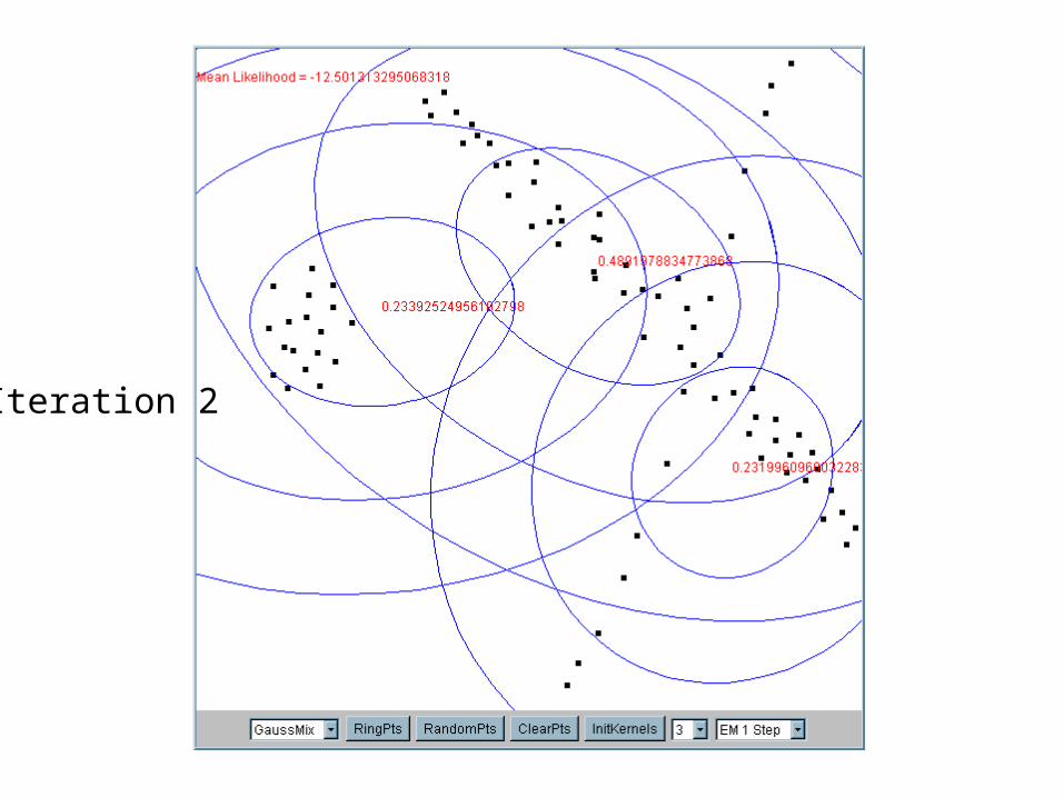
Iteration 2

Iteration 5

Iteration 25

Nearest Neighbor ClusteringNearest Neighbor ClusteringNot to be confused with Nearest Neighbor Not to be confused with Nearest Neighbor ClassificationClassification
• Items are iteratively merged into the existing clusters that are closest.
• Incremental
• Threshold, t, used to determine if items are added to existing clusters or a new cluster is created.
What happens if the data is streaming…

10
1 2 3 4 5 6 7 8 9 10
1
2
3
4
5
6
7
8
9
Threshold t
t 1
2
10
1 2 3 4 5 6 7 8 9 10
1
2
3
4
5
6
7
8
9
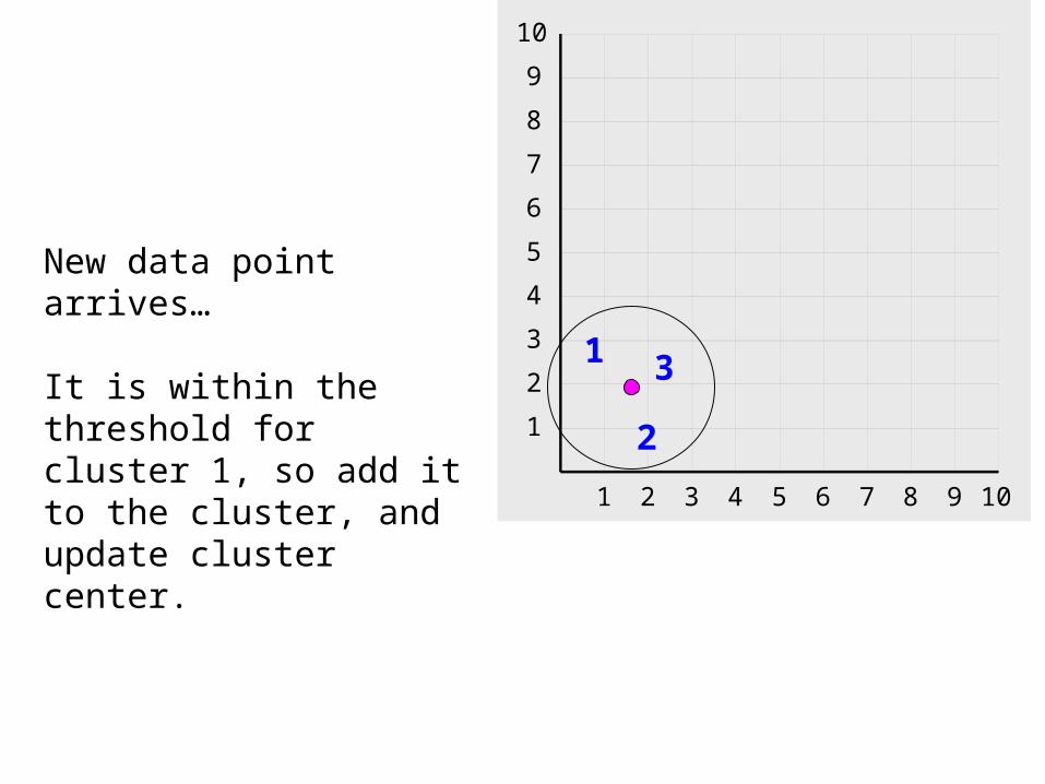
New data point arrives…
It is within the threshold for cluster 1, so add it to the cluster, and update cluster center.
1
2
3
10
1 2 3 4 5 6 7 8 9 10
1
2
3
4
5
6
7
8
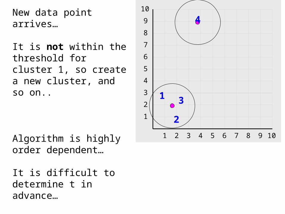
9New data point arrives…
It is not within the threshold for cluster 1, so create a new cluster, and so on..
1
2
3
4
Algorithm is highly order dependent…
It is difficult to determine t in advance…
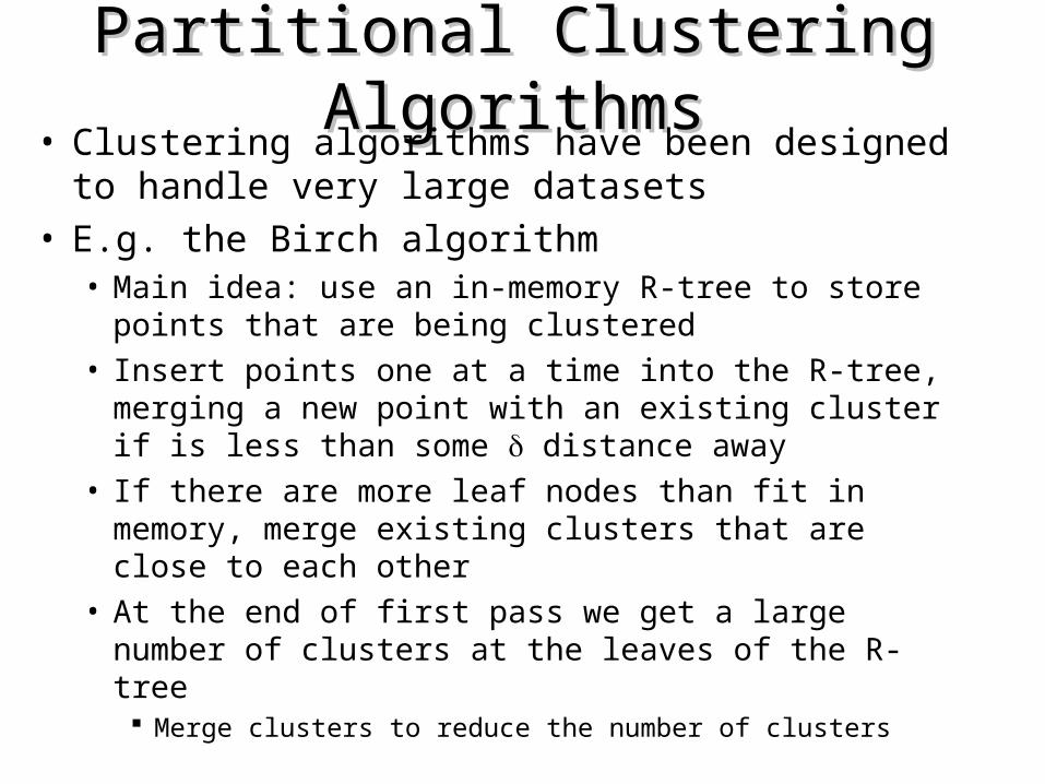
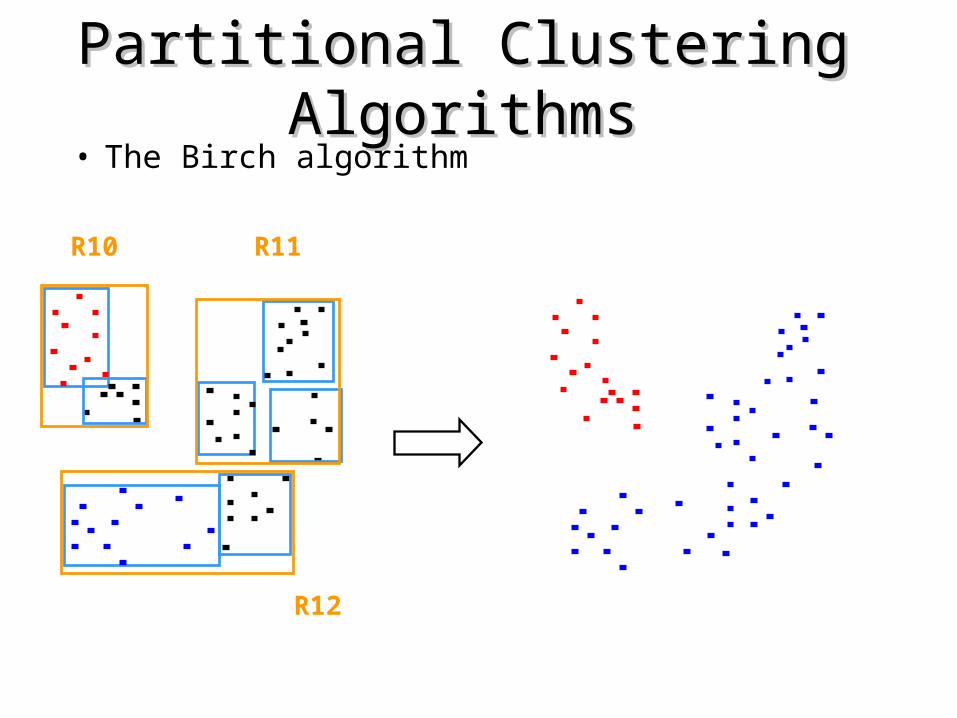
Partitional Clustering AlgorithmsPartitional Clustering Algorithms• Clustering algorithms have been designed to handle
very large datasets• E.g. the Birch algorithm
• Main idea: use an in-memory R-tree to store points that are being clustered
• Insert points one at a time into the R-tree, merging a new point with an existing cluster if is less than some distance away
• If there are more leaf nodes than fit in memory, merge existing clusters that are close to each other
• At the end of first pass we get a large number of clusters at the leaves of the R-tree Merge clusters to reduce the number of clusters
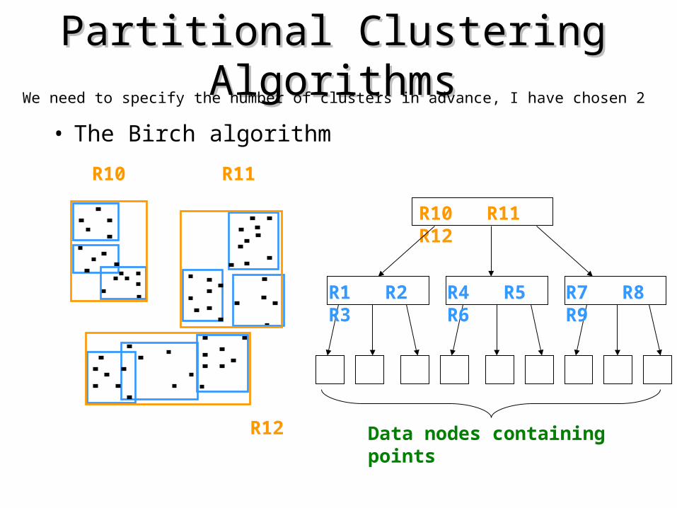
Partitional Clustering AlgorithmsPartitional Clustering Algorithms
• The Birch algorithm
R10 R11 R12
R1 R2 R3 R4 R5 R6 R7 R8 R9
Data nodes containing points
R10 R11
R12
We need to specify the number of clusters in advance, I have chosen 2
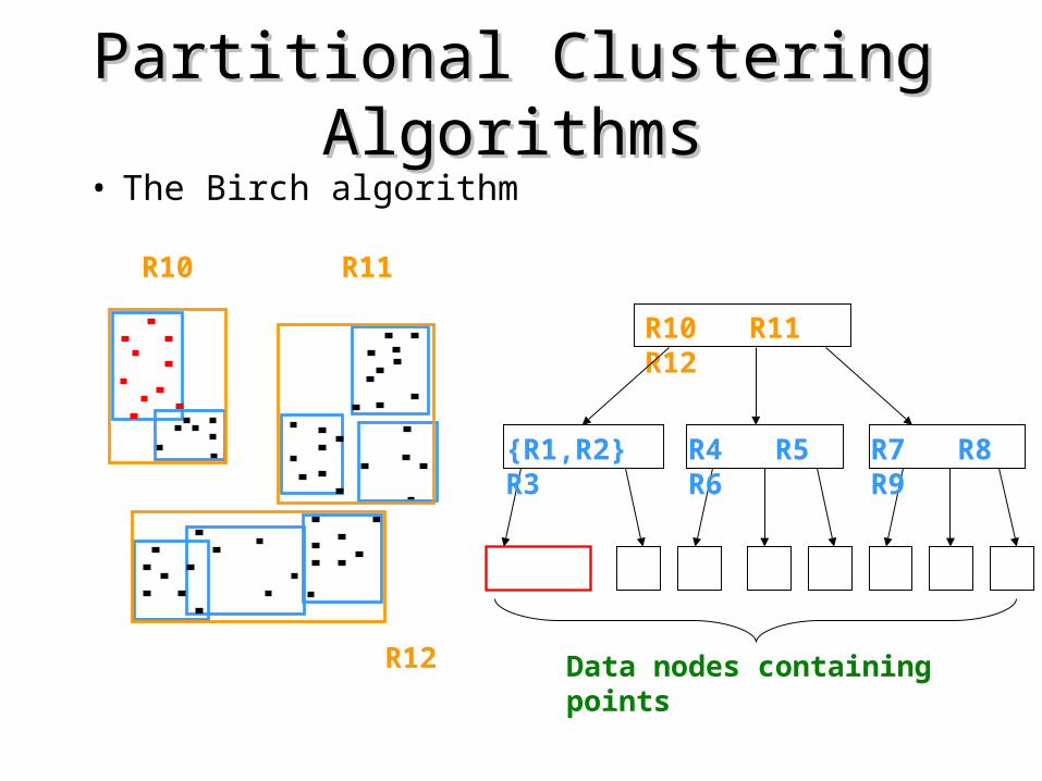
Partitional Clustering AlgorithmsPartitional Clustering Algorithms• The Birch algorithm
R10 R11 R12
{R1,R2} R3 R4 R5 R6 R7 R8 R9
Data nodes containing points
R10 R11
R12
Partitional Clustering AlgorithmsPartitional Clustering Algorithms• The Birch algorithm
R10 R11
R12
10
1 2 3 4 5 6 7 8 9 10
1
2
3
4
5
6
7
8
9
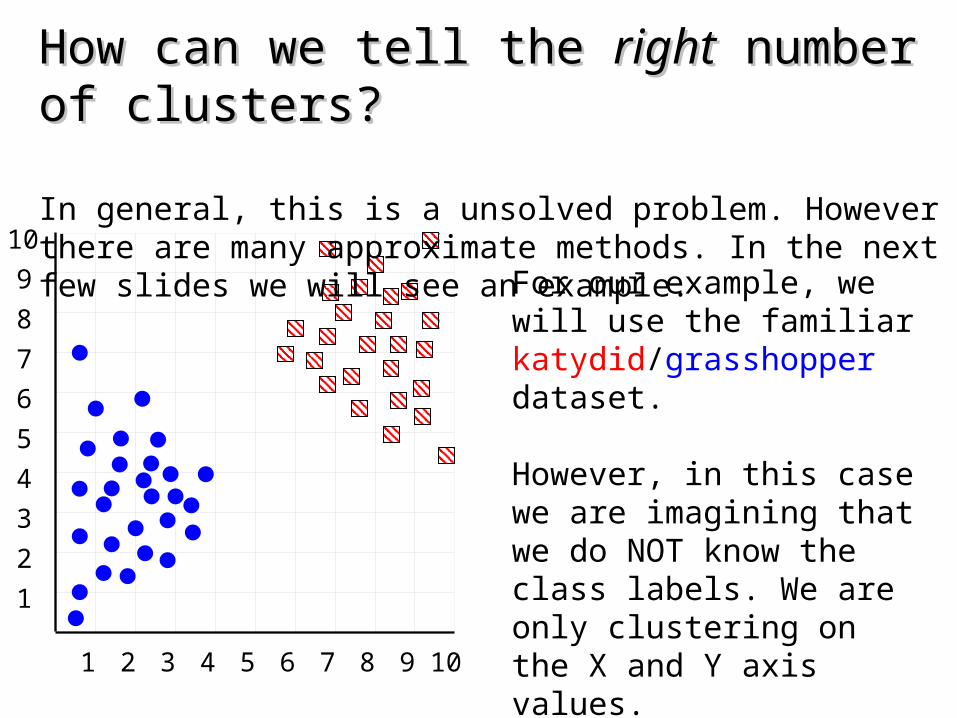
How can we tell the How can we tell the rightright number of clusters? number of clusters?
In general, this is a unsolved problem. However there are many approximate methods. In the next few slides we will see an example.
For our example, we will use the familiar katydid/grasshopper dataset.
However, in this case we are imagining that we do NOT know the class labels. We are only clustering on the X and Y axis values.

1 2 3 4 5 6 7 8 9 10
When k = 1, the objective function is 873.0

1 2 3 4 5 6 7 8 9 10
When k = 2, the objective function is 173.1
1 2 3 4 5 6 7 8 9 10
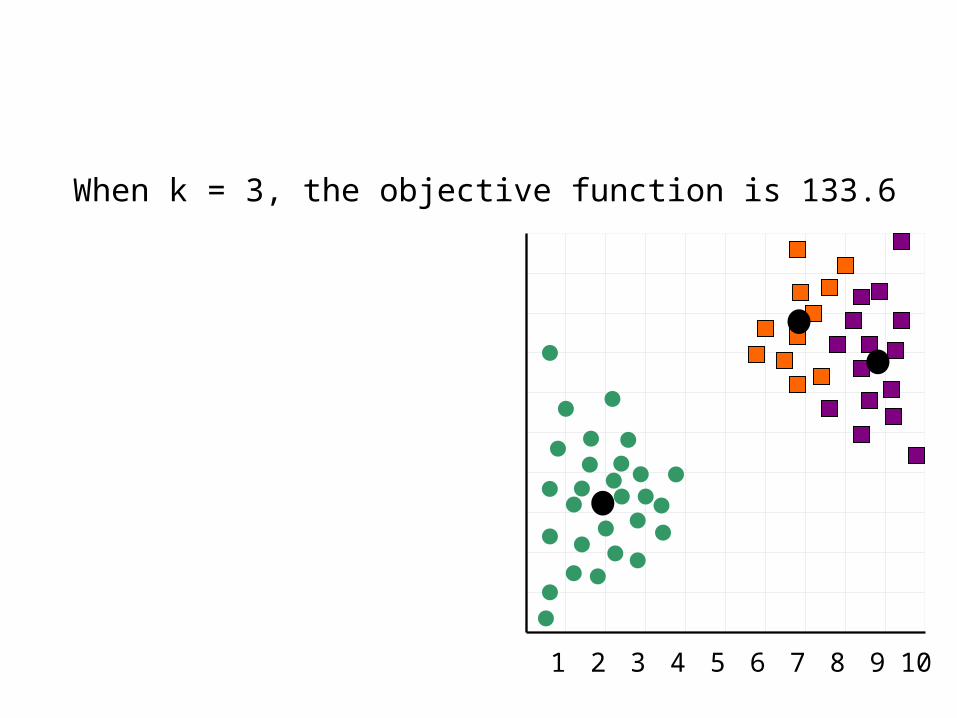
When k = 3, the objective function is 133.6

0.00E+00
1.00E+02
2.00E+02
3.00E+02
4.00E+02
5.00E+02
6.00E+02
7.00E+02
8.00E+02
9.00E+02
1.00E+03
1 2 3 4 5 6
We can plot the objective function values for k equals 1 to 6…
The abrupt change at k = 2, is highly suggestive of two clusters in the data. This technique for determining the number of clusters is known as “knee finding” or “elbow finding”.
Note that the results are not always as clear cut as in this toy example
k
Obj
ecti
ve F
unct
ion
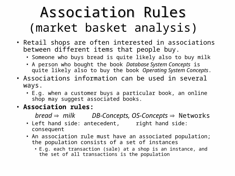
Association RulesAssociation Rules(market basket analysis)
• Retail shops are often interested in associations between different items that people buy. • Someone who buys bread is quite likely also to buy milk• A person who bought the book Database System Concepts is quite
likely also to buy the book Operating System Concepts.
• Associations information can be used in several ways. • E.g. when a customer buys a particular book, an online shop may
suggest associated books.
• Association rules: bread milk DB-Concepts, OS-Concepts Networks• Left hand side: antecedent, right hand side: consequent• An association rule must have an associated population; the
population consists of a set of instances• E.g. each transaction (sale) at a shop is an instance, and the set of all
transactions is the population

Association Rule DefinitionsAssociation Rule Definitions
• Set of items: I={I1,I2,…,Im}• Transactions: D={t1,t2, …, tn}, tj I• Itemset: {Ii1,Ii2, …, Iik} I• Support of an itemset: Percentage of
transactions which contain that itemset.• Large (Frequent) itemset: Itemset whose
number of occurrences is above a threshold.
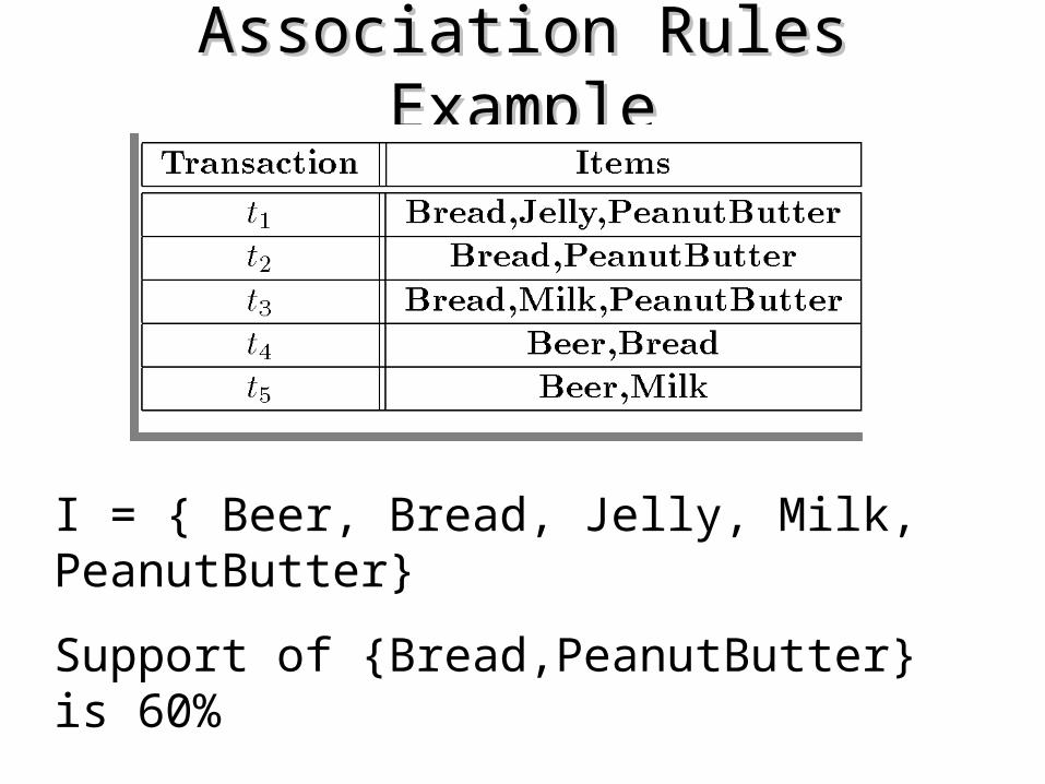
Association Rules ExampleAssociation Rules Example
I = { Beer, Bread, Jelly, Milk, PeanutButter}
Support of {Bread,PeanutButter} is 60%
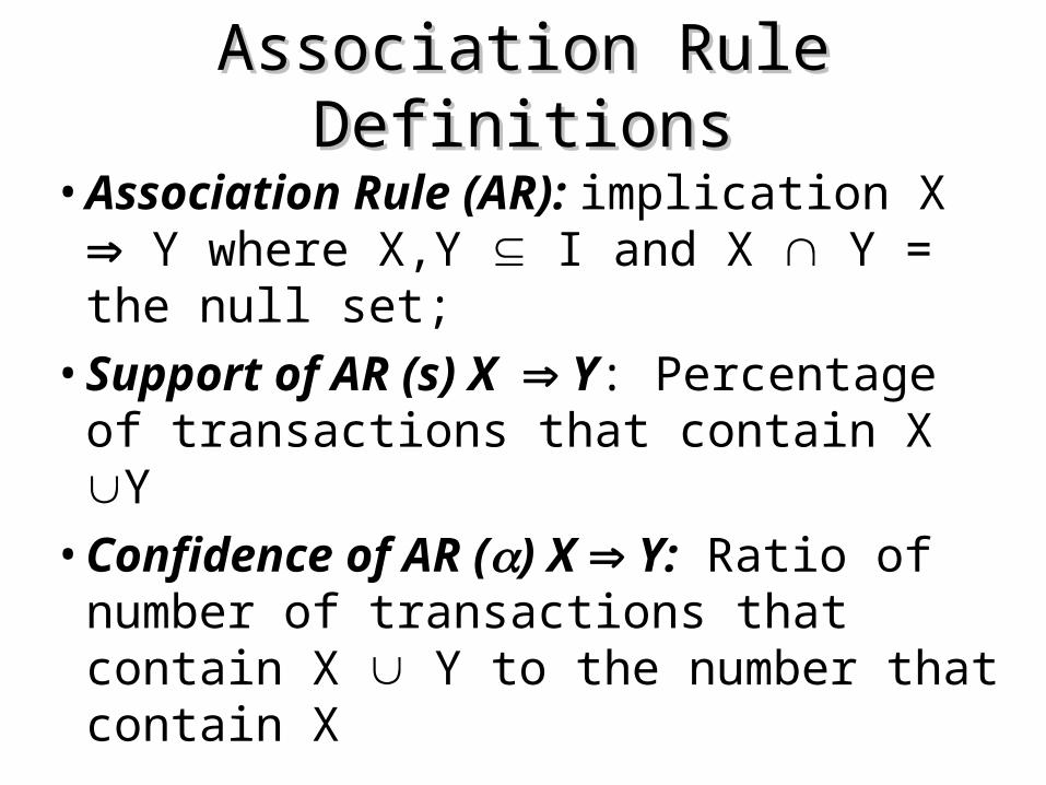
Association Rule DefinitionsAssociation Rule Definitions
• Association Rule (AR): implication X Y where X,Y I and X Y = the null set;
• Support of AR (s) X Y: Percentage of transactions that contain X Y
• Confidence of AR () X Y: Ratio of number of transactions that contain X Y to the number that contain X

Association Rules ExampleAssociation Rules Example
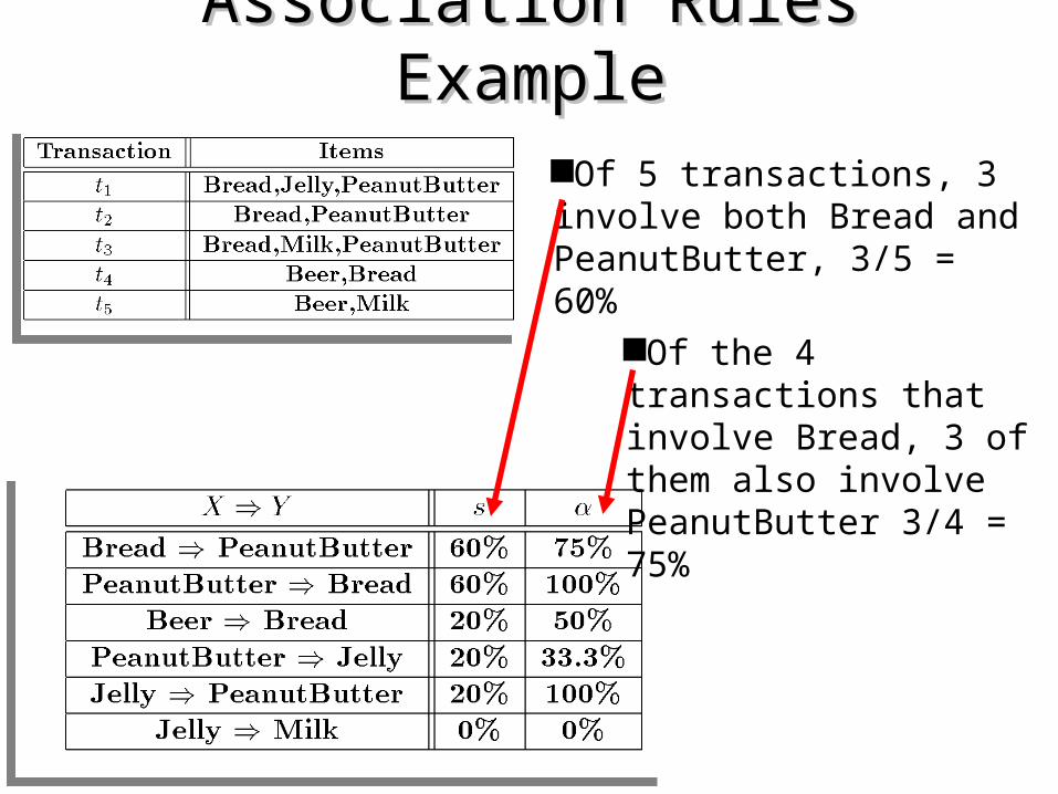
Association Rules ExampleAssociation Rules Example
Of 5 transactions, 3 involve both Bread and PeanutButter, 3/5 = 60%
Of the 4 transactions that involve Bread, 3 of them also involve PeanutButter 3/4 = 75%
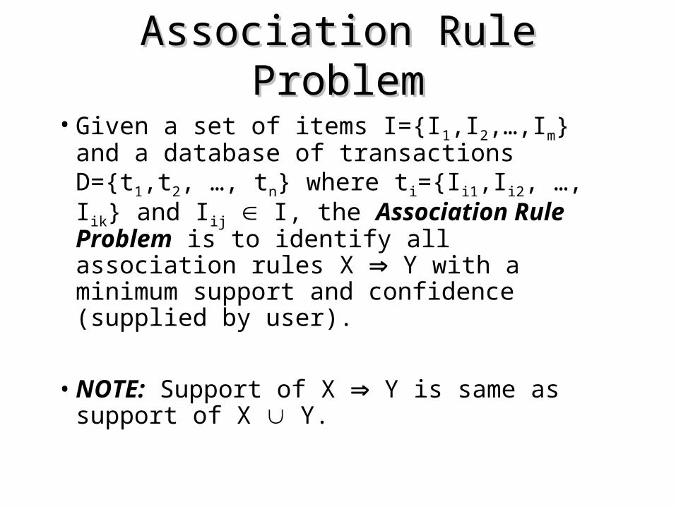
Association Rule ProblemAssociation Rule Problem
• Given a set of items I={I1,I2,…,Im} and a database of transactions D={t1,t2, …, tn} where ti={Ii1,Ii2, …, Iik} and Iij I, the Association Rule Problem is to identify all association rules X Y with a minimum support and confidence (supplied by user).
• NOTE: Support of X Y is same as support of X Y.
Association Rule Algorithm Association Rule Algorithm (Basic Idea)(Basic Idea)
1. Find Large Itemsets.2. Generate rules from frequent itemsets.
This is the simple naïve algorithm, better algorithms exist.

Association Rule AlgorithmAssociation Rule Algorithm We are generally only interested in association rules with
reasonably high support (e.g. support of 2% or greater)
Naïve algorithm
1. Consider all possible sets of relevant items.
2. For each set find its support (i.e. count how many transactions purchase all items in the set).
• Large itemsets: sets with sufficiently high support
• Use large itemsets to generate association rules.
• From itemset A generate the rule A - {b} b for each b A.
• Support of rule = support (A).
• Confidence of rule = support (A ) / support (A - {b})

• From itemset A generate the rule A - {b} b for each b A.
• Support of rule = support (A).
• Confidence of rule = support (A ) / support (A - {b})
Lets say itemset A = {Bread, Butter, Milk}
Then A - {b} b for each b A includes 3 possibilities
{Bread, Butter} Milk
{Bread, Milk} Butter
{Butter, Milk} Bread
Apriori AlgorithmApriori Algorithm
• Large Itemset Property:Any subset of a large itemset is
large.• Contrapositive:
If an itemset is not large, none of its supersets are large.
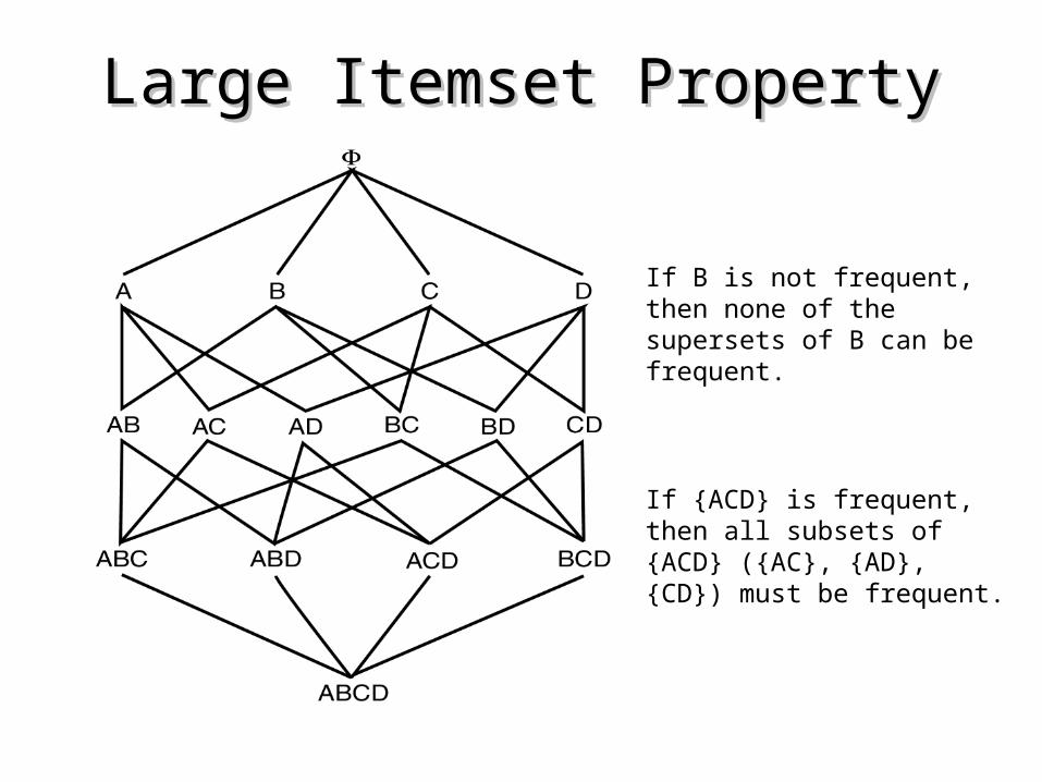
Large Itemset PropertyLarge Itemset Property
If B is not frequent, then none of the supersets of B can be frequent.
If {ACD} is frequent, then all subsets of {ACD} ({AC}, {AD}, {CD}) must be frequent.
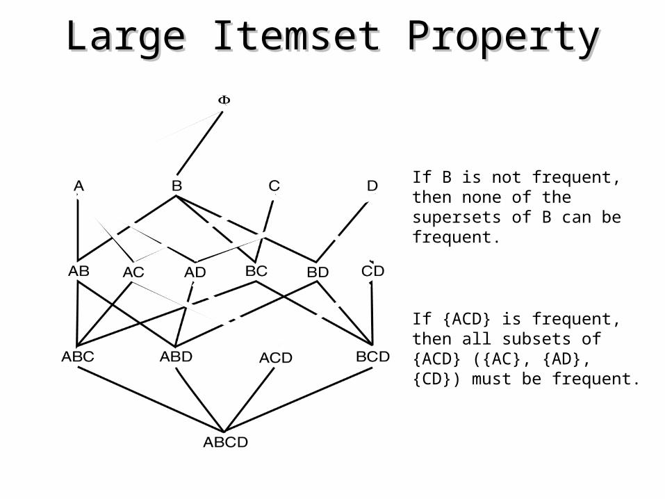
Large Itemset PropertyLarge Itemset Property
If B is not frequent, then none of the supersets of B can be frequent.
If {ACD} is frequent, then all subsets of {ACD} ({AC}, {AD}, {CD}) must be frequent.

ConclusionsConclusions• We have learned about the 3 major data mining/machine learning algorithms.• Almost all data mining research is in these 3 areas, or is a minor extension of one or more of them.
• For further study, I recommend.• Proceedings of SIGKDD, IEEE ICDM, SIAM SDM• Data Mining: Concepts and Techniques (Jiawei Han and Micheline Kamber)• Data Mining: Introductory and Advanced Topics (Margaret Dunham)