The Magellan Adaptive Secondary AO System IFS

Proposal Outline

Laird Close (PI), Victor Gasho (PM), Derek Kopon (Optical eng.), Jared Males (Software and simulations),

Kate Brutlag (Science) Steward Observatory, University of Arizona

Alan Uomoto (Magellan PM), Tyson Hare (Mech eng.) OCIW, Pasadena, CA

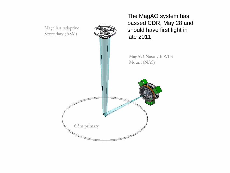
Magellan Adaptive Secondary (ASM)

MagAO Nasmyth WFS Mount (NAS)

6.5m primary

The MagAO system has passed CDR, May 28 and should have first light in late 2011.

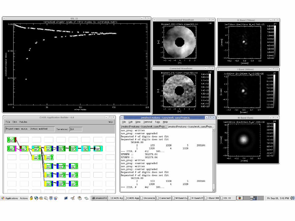
Our simulations suggest that MagAO will have some correction in the optical

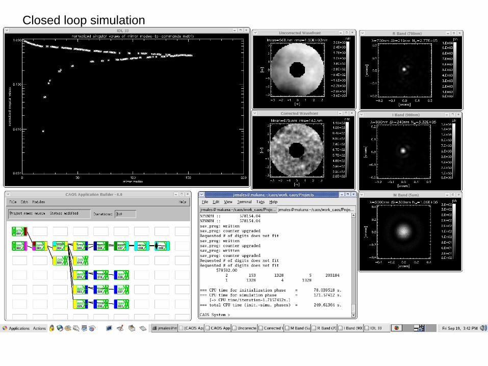
Closed loop simulation

Note the moderate Strehl at 0.7μm

AO OFF

AO ON

~25% SR

No SeeingVisible (0.7μm) Lab Test Results (0.7”

seeing)

These Strehls SURPASS OUR PREDICTED PERFORMANCE at 0.7μm

With ~10-20% Strelhs at 0.7μm and 20 mas resolutions a MagAO IFS

would be unique in world

1. Nothing like this in operation today.

2. Only similar future system is Palm3000 (2010? NGS, then LGS 2011?) at the 5m Palomar system in the north. SWIFT is palm3000’s IFS with R~3500, 0.65-1.05μm 44x89 spaxials: 80,160,240 mas. So spatial resolutions are >80mas (4x worst than MagAO IFS)

3. There is also the Keck NGAO system, ~2015-2016 if large amounts of funding is found

Why do we want to couple an IFS to the Magellan AO system?

IFS point design issues:

1. Need to have fibers sample the 20mas diffraction-limit at 0.7um

2. Need to have coarser ~60mas platescale

3. Need to have alignment camera and steering mirror

4. Need as many spaxials as possible

5. Need to cover 0.6-1.1um with high QE

6. Simultaneous PSF calibration

1. Need f/149 beam to feed 30x30 125um microarray coupled to 62.5um core/125um clad low OH “dry” Multi-Mode fibers

2. Need to have a f/49 beam as well

3. Use 5/95 fold mirror to feed IFS, then CCD47 as guider closed loop on steering mirror.

4. 4096/6pix/fiber ~ 680 =26x26 design fits.

5. LDSS3 red-sensitive spectrograph with fibers reformatted to f/11 longslit mode –700 4k spectra!

6. Use CCD47 for simultaneous PSF calibration

Top-level requirement Design solution

Adaptive y (ASM)

MagAO Nasmyth WFS Mount (NAS)

6.5m primary

IFS Fiber bundle

LDSS3 Spectrograph (not mounted on a port in IFS mode)

Cartoon Overview of the MagAO IFS Concept (note the IFS can be used with Mirac4 still mounted).

Preliminary 20 mas Fiber Coupling Lens Design

Modified from http://star-www.dur.ac.uk/~jra/integral_field.html

LDSS3

Preliminary 20 mas Fiber Coupling Lens Cartoon

Modified from http://star-www.dur.ac.uk/~jra/integral_field.html

f/149f/5

f/5 f/11

125um microlens array

62.5 um

LDSS3MagAO

Relay Lens Design

Derek Kopon8/22/09

Design Parameters

• x3 magnification (F/49 to F/148.8)• 0.6-1.1 um• 1 arcsec field (corner to corner)• Lens element(s) located 3 inches before nominal CCD47

F/45 focus• F/148.8 focus located 200mm past nominal F/45 focus• No lenslets included, but commercially available• Common glasses

3x expander Doublet

All sphere design converts f/49 to f/149, enables 23 mas sampling on square 125 μm microlenslet array

• 5 deg Zenith angle• Big circle is the diffraction limit (first Airy minimum of 0.6um)• Little circle is fiber (100 um diameter) – so diffraction-limited • Design can be optimized further, but is already diffraction limited

A 125 um square microlens array gives a 23 mas/spaxials

Spot diagrams at 50 deg Zenith. Current ADC design leaves only minor chromatic spread from 0.6-1.1 μm. This small a spread will not effect the spatial image quality of the IFS data cube.

Preliminary Mechanical Design

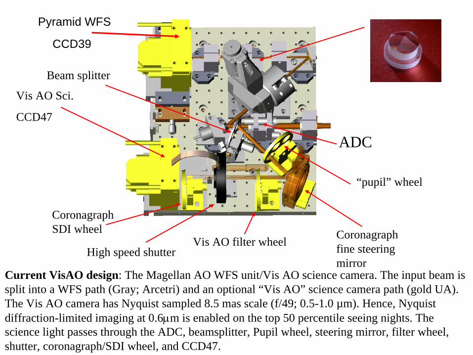
Pyramid WFS

CCD39

Current VisAO design: The Magellan AO WFS unit/Vis AO science camera. The input beam is split into a WFS path (Gray; Arcetri) and an optional “Vis AO” science camera path (gold UA). The Vis AO camera has Nyquist sampled 8.5 mas scale (f/49; 0.5-1.0 µm). Hence, Nyquist diffraction-limited imaging at 0.6μm is enabled on the top 50 percentile seeing nights. The science light passes through the ADC, beamsplitter, Pupil wheel, steering mirror, filter wheel, shutter, coronagraph/SDI wheel, and CCD47.

Vis AO Sci.

CCD47

Coronagraph SDI wheel Coronagraph

fine steering mirror

Vis AO filter wheel

ADC

High speed shutter

“pupil” wheel

Beam splitter

IFS with 69 mas/spaxials (“coarse” f/45 mode)

IFS with 23 mas spaxials (fine f/149 mode) with 3x expander lens in beam.

The LDSS3 spectrograph

LDSS3

Red sensitive, high QE, 0.6-1.05μm R~1800

spectra of 680 objects at once – shown is here

an R=18.5 esdM7.5 VLM star 2M1227 (10

min exposure, on LDSS3)

example from Burgasser et al. ApJ 657 494

Science Case #1

Circumstellar Disk Morphology

At 20mas resolutions we can actually spatially map the forbidden line emissions from the gas in

the disk (by Kate Brutlag)

Down sampled at LDSS3’s resolutions – for continuum subtraction

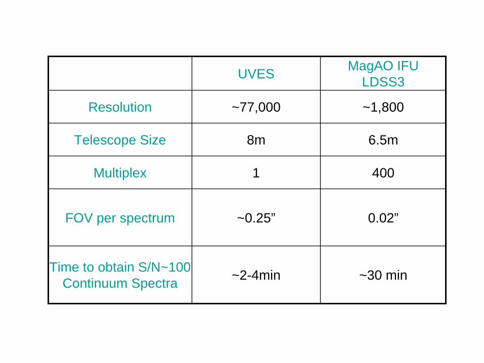
UVES MagAO IFULDSS3

Resolution ~77,000 ~1,800

Telescope Size 8m 6.5m

Multiplex 1 400

FOV per spectrum ~0.25” 0.02”

Time to obtain S/N~100 Continuum Spectra ~2-4min ~30 min

The range of expected simulated PSFs for VisAO

Simulated [OI] Emission from Disk of HD101412 Convolved with PSF

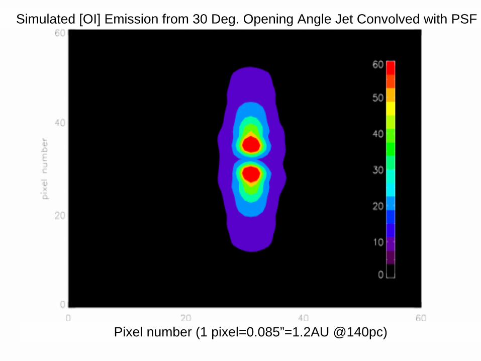
Pixel number (1 pixel=0.085”=1.2AU @140pc)

Simulated [OI] Emission from Disk of HD101412 Convolved with PSF

With 5-10AU Gap

Pixel number (1 pixel=0.085”=1.2AU @140pc)

Pixel number (1 pixel=0.085”=1.2AU @140pc)

Simulated [OI] Emission from 30 Deg. Opening Angle Jet Convolved with PSF

PSF for Model Convolution

PSF for Model Deconvolution

40% PSF Mismatch

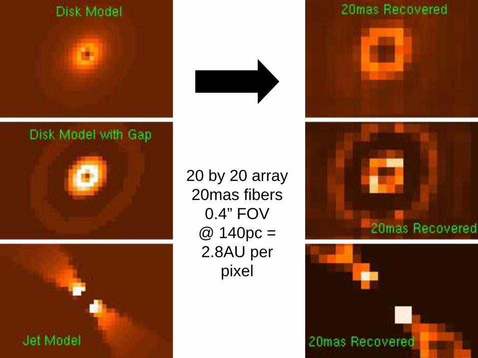
20 by 20 array20mas fibers

0.4” FOV@ 140pc = 2.8AU per

pixel

Jet + Disk: 10:1 Flux Scaling Model

Jet + Disk: 10:1 Flux Scaling Model after Deconvolution

More Science Cases

#2. Resolving tight astrometric binaries and the High-mass Mass-Function

Histogram of Candidate Binaries with Calculated Astrometric Orbits and Declinations<40

0

20

40

60

80

100

120

140

160

180

200

0.01 0.02 0.03 0.04 0.05 0.06 0.07 0.08 0.09 0.10 0.11 0.12 0.13 0.14 0.15 0.16 0.17 0.18 0.19 0.20

Separation (in arcseconds)

Calibrating the High Mass MF by accurate typing of the primary and secondary of astrometric binaries, 97% of which have separations <0.2”

Ephemerides Catalog341 Candidates with:

• Separations < 1 arcsecond in 2011

• Calculated Astrometric Orbits

• Declinations < +40• 330 have separations < 0.2”• 5<V<11 mag• ΔV<2

More Science Cases

#3. Highest resolution Black hole “sphere of influence” observations

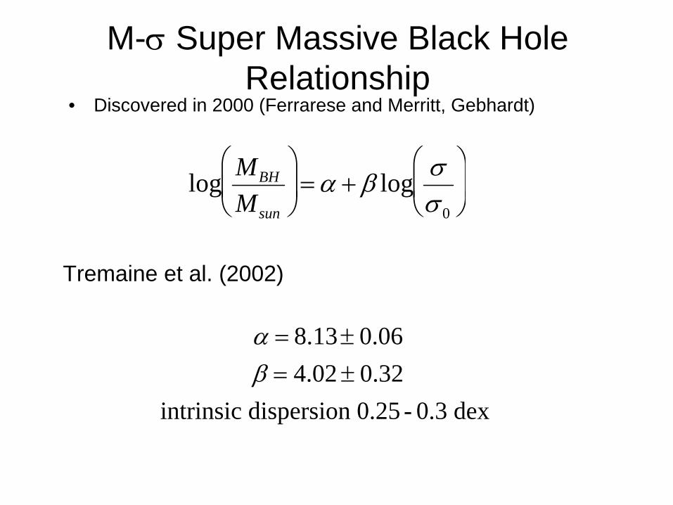
• Discovered in 2000 (Ferrarese and Merritt, Gebhardt)

log MBH

Msun

⎛

⎝ ⎜

⎞

⎠ ⎟ = α + β log σ

σ 0

⎛

⎝ ⎜

⎞

⎠ ⎟

Tremaine et al. (2002)

α = 8.13± 0.06β = 4.02 ± 0.32

intrinsic dispersion 0.25 - 0.3 dex

M-σ

Super Massive Black Hole Relationship

Accurate Black Hole Masses through high spatial resolution probe of BH “Sphere of Influence”

• Spatial resolution: need to resolve the black hole's dynamical sphere of influence to get mass rg = GMBH /σ2

• If you see the Keplerian rise in the rotation curve, mass determination becomes more accurate

Simulation: 108 Msun BH at 20 Mpc, inclination 60 deg to line of sight (Keck NGAO study figure)

MagAO IFS

VisAO advantage for BH mass VisAO advantage for BH mass determinationdetermination

• With MagAO, diffraction-limited PSF core at Ca II triplet is major improvement in spatial resolution (assuming a bright enough guide star in the AGN core can be used for MagAO guiding)

– Enables many more low-mass black holes to be detected

– Better for resolving rg in nearby galaxies, leading to more accurate measurements

– MagAO CaII or Hα

can study high-mass distant galaxies to pin down extreme end of M-σ

relation

– Minimum BH mass detectable distance is >2x better with MagAO compared to 10-m AO today -- assuming local M-σ

relation and >2 resolution elements across rg

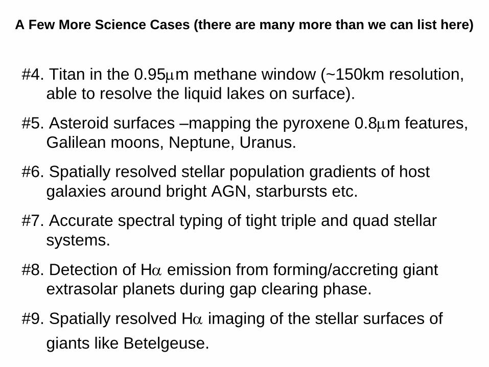
A Few More Science Cases (there are many more than we can list here)

#4. Titan in the 0.95μm methane window (~150km resolution, able to resolve the liquid lakes on surface).

#5. Asteroid surfaces –mapping the pyroxene 0.8μm features, Galilean moons, Neptune, Uranus.

#6. Spatially resolved stellar population gradients of host galaxies around bright AGN, starbursts etc.

#7. Accurate spectral typing of tight triple and quad stellar systems.

#8. Detection of Hα

emission from forming/accreting giant extrasolar planets during gap clearing phase.

#9. Spatially resolved Hα

imaging of the stellar surfaces of giants like Betelgeuse.

Schedule for ATI proposal Timeline

1. Delivery of documents to SAC - today2. Present plan to the SAC on Sept. 10 telecon.3. Andy give (hopefully) positive review to Council

during the Sept 18 meeting.4. Get positive statements from SAC and council in

Sept. 5. Submit ATI proposal in late October (Due Nov 1,

2009)