the life cycle of plants in india and...
TRANSCRIPT
1
The Life Cycle of Plants in India and Mexico*
Chang-Tai Hsieh University of Chicago and NBER
Peter J. Klenow
Stanford University, SIEPR and NBER
April 2012
Preliminary
Abstract
In the U.S., the average 40 year old plant employs almost eight times as many workers as the typical plant five years or younger. In contrast, surviving Indian plants exhibit little growth in terms of either employment or output. Indian plants start smaller and stay smaller. Most Indian manufacturing employment is at informal plants with fewer than 10 workers. In the U.S. most workers are at plants with more than 800 workers. Mexico is intermediate to India and the U.S. in these respects. The divergence in plant dynamics suggests lower investments by Indian and Mexican plants in process efficiency, quality, and variety, and in accessing markets at home and abroad. In simple GE models, we find that the difference in life cycle dynamics could lower aggregate manufacturing productivity on the order of 25%.
* We benefited from the superlative research assistance of Siddharth Kothari, Huiyu Li, and Pedro Jose Martinez Alanis. Ariel Burstein generously shared his Matlab programs. The paper incorporates many helpful comments from seminar participants and discussants. Hsieh thanks Chicago’s Initiative for Global Markets and the Templeton Foundation and Klenow thanks the Stanford Institute for Economic Policy Research for financial support. Emails: [email protected] and [email protected]. The results have been screened by the U.S. Census Bureau and Mexico’s INEGI to ensure no confidential information is released.
2
I. Introduction A well-established fact in the U.S. is that new businesses tend to start small and grow
substantially as they age.1 For example, forty year old manufacturing plants are almost eight
times larger than plants under the age of five in terms of employment (See Figure 1). Atkeson
and Kehoe (2005) suggest that this life cycle is driven by the accumulation of plant-specific
organizational capital. According to this interpretation, establishments grow with age as they
invest in new technologies, develop new markets, and produce a wider array of higher quality
products. Foster, Haltiwanger, and Syverson (2012) show that, even in commodity-like markets
(such as white bread), establishment growth is largely driven by rising demand for the plant’s
products as it ages.
This paper examines the importance of the accumulation of establishment-specific
intangible capital over the life cycle for understanding differences in aggregate TFP between
poor and rich countries. Specifically, we focus on a comparison of the life cycle in the Indian
and Mexican manufacturing sectors with the U.S. We choose India and Mexico because they
have comprehensive micro-data on manufacturing establishments that allows us to measure the
life cycle properly. Importantly, the data we use captures the large informal sector (as well as
the formal establishments) in these countries. Most other available datasets, such as the data on
Chinese manufacturing we used in Hsieh and Klenow (2009), are inadequate for measuring the
life cycle as they only survey large establishments.
As preliminary evidence, consider the relationship between establishment employment
and age in India and Mexico shown in Figure 1. In contrast to the U.S., in India old plants are no
larger than young plants. In Mexico, 25 year old plants are twice the size of new plants, not far
from the U.S. pattern. What differs between the U.S. and Mexico is that 40 year old plants in
Mexico are no larger than 25 year old plants, while 40 year old U.S. plants are almost four times
larger than their 25 year old counterparts. These facts are consistent with establishments
accumulating less organizational capital in India and Mexico than in the U.S.
Why would firms in India and Mexico invest less in organizational capital? The returns
to such investments might be lower in India and Mexico for a multitude of reasons. Large plants
could face higher taxes or higher labor costs. Levy (2008) argues that payroll taxes in Mexico
1 See, for example, Dunne, Roberts, and Samuelson (1989) and Davis, Haltiwanger, and Schuh (1996). Cabral and Matta (2003) provide similar evidence from Portugal.
3
are more stringently enforced on large plants. Bloom et. al. (2011) suggest difficulty in contract
enforcement makes it costly to hire the skilled managers necessary to grow in India. Financial
constraints are another possible contributor. Many authors have modeled the U.S. life cycle as
the result of relaxing financial constraints as the establishment grows.2 If large establishments
in India and Mexico still face financial constraints, this would diminish their incentive to grow.
Another force might be higher transportation and trade costs that make it more difficult for high
productivity establishments to reach more distant (internal or external) markets. Consistent with
these stories, the gap in the average revenue product of resources between high and low
productivity establishments is five to six times larger in India and Mexico than in the U.S. – as if
high productivity establishments face higher taxes or factor costs in India and Mexico.
To gauge the potential effect of the life cycle on aggregate productivity, we examine
simple GE models based on Melitz (2003) and Atkeson and Burstein (2010). We focus on three
mechanisms. First, if post-entry investment in intangible capital is lower in India and Mexico,
the productivity of older plants will be correspondingly lower. Second, lower productivity of
older plants due to lower life-cycle growth reduces the competition posed by incumbents to
young establishments. For this reason, slower life-cycle growth can boost the flow of entrants
and reduce average establishment size. Third, if potential entrants have some information about
their productivity ex ante, a larger flow of entrants may bring in marginal entrants who are less
productive than infra-marginal entrants. When moving from the U.S. life cycle to the Indian life
cycle, the net effect of these three forces could plausibly account for a 25% drop in aggregate
TFP and a 50% decline in establishment size.
The paper proceeds as follows. Section II describes the data. Section III presents the
basic facts about the life cycle of plants in India, Mexico, and the U.S. Section IV provides
suggestive evidence on forces that might be lowering the return to intangible capital in India and
Mexico. Section V lays out a GE model of heterogeneous firms with life-cycle productivity to
illustrate the potential consequences for aggregate productivity of differences in the life-cycle
profile between India and the U.S. Section VI concludes.
2 Cooley and Quadrini (2001), Albuquerque and Hopenhayn (2002), Cabral and Matta (2003), and Clementi and Hopenhayn (2006) are examples of models with this mechanism.
4
II. Data To measure the life cycle of a cohort of establishments, we need data that is
representative across the age distribution. A typical establishment-level dataset has information
only on plants above a certain size threshold. This is problematic for measuring the life cycle if
most new establishments are small. Our analysis focuses on the U.S., Mexico, and India as these
countries have establishment level data that are representative across the full size distribution of
manufacturing establishments.
For the U.S., we use the data from the quinquennial Manufacturing Census. This data is
available every five years from 1963 through 2002. The variables we use from the U.S. Census
are the wage bill, number of workers, value-added, the book value of the capital stock, and the
industry (four digit SIC from 1963 to 1997 and six digit NAICS in 2002). In each year, there are
slightly more than 400 industries. The U.S. Census does not provide information on the
establishment’s age. We impute an establishment’s age based on when the establishment
appeared in the Census for the first time. We have data every five years starting in 1963 so we
group establishments into five-year age groupings. For our analysis, we will use the Censuses
from 1992, 1997, and 2002 as these are the years with the most complete age information. We
also keep the administrative records in our sample. These are small plants where the Census
Bureau imputes plant employment and output from payroll data (using industry-wide averages of
the ratio of output and employment to the wage bill). In Hsieh and Klenow (2009) we omitted
administrative records as our focus there was on the dispersion of the ratio of plant output to
inputs. Here, our main focus is on plant employment which is not likely to be significantly
biased in the administrative record establishments.
The data we use for Indian manufacturing is the Annual Survey of Industries (ASI) and
the Survey of Informal Establishments of the National Sample Survey (NSS). The ASI is a
census of manufacturing establishments with more than 100 employees and a random sample of
formally registered establishments with less than 100 employees.3 The NSS is a survey of
informal establishments conducted once every five years as one of the modules of the Indian
National Sample Survey. The ASI and the NSS collect data over the fiscal year (July 1 through
June 30). We have the ASI for every year from 1980-81 to 2007-2008. The NSS is only
3 One third of the formal plants with less than 100 workers were surveyed in the ASI prior to 1994-95. The sampling probability of the smaller plants in the ASI decreased (to roughly one seventh) after 1994-95.
5
available for four years: 1989-1990, 1994-1995, 1999-2000, and 2005-2006. Our analysis will
therefore focus on the years for which both the ASI and the NSS are available, and we will refer
to the combined dataset as the ASI-NSS.
To make the Indian data comparable to the U.S., we restrict the analysis to sectors that
are also classified as manufacturing in the U.S. data.4 The variables we use are the number of
paid employees, contract workers, unpaid workers, wage and non-wage compensation (for the
establishments with paid employees or contract workers), total capital stock (and two of its
components -- machinery and equipment and value of land), value added, industry, and
establishment age.5 The ASI and the NSS use the same industry classification (about 400
industries each year). Establishment age is available for all years in the ASI but only available in
1989-90 and 1994-95 in the NSS. Establishment identifiers are provided in the ASI starting in
1998-99; the NSS does not have establishment identifiers. We also use information in the ASI
on electricity provided by the plant’s generator and purchased from the electric grid (the NSS
does not have information on generators).
For Mexico, we use data from the Mexican Economic Census. The Economic Census is
conducted every five years by Mexico's National Statistical Institute (known by its Spanish
acronym INEGI). The Census is a complete enumeration of all fixed establishments in Mexico.
The only establishments not in the Economic Census are street vendors, public sector entities,
and establishments in the agricultural sector. We have access to the micro-data of Mexican
Censuses from 1998, 2003, and 2008. To make the Mexican data comparable to the U.S., we
restrict our attention to establishments in the manufacturing sector.6 The variables we use from
this data are the number of paid employees, contract workers, unpaid workers, wage bill, labor
taxes (paid to Mexico’s Social Security Agency) and other non-wage compensation, total capital
stock, value-added, establishment age, and industry (roughly 350 industries in manufacturing).
In 2003, we also have information on machinery and equipment capital and the value of the land
4 This primarily removes auto and bicycle repair shops that are classified as manufacturing in the Indian data. Repair shops account for roughly 20 percent of all establishments in the Indian data. 5 The ASI does not have information on unpaid workers in 1999-2000. Unpaid workers account for 0.8 to 1.5 percent of total employment in the ASI plants in 1989-90, 1994-95, and 2005-06. 6 There are two industries classified as manufacturing in 1998 (CMAP 311407 and 321201) but later reclassified as agriculture in 2003 and 2008. We drop these industries from the 1998 sample.

6
used by the establishment. Finally, although the Mexican data is a complete census, there are no
establishment identifiers in the data and there is not enough information in the data to link
establishments between census years.
Table 1 presents the number of establishments and total employment in our data.7 We
focus on establishments rather than firms. We do not have information on firms in the Indian
and Mexican data. The number of workers in India and Mexico includes unpaid and contract
workers. According to Table 1, most Indian manufacturing establishments are in the informal
sector (i.e., in the NSS). Though informal establishments are smaller, they still account for 80
percent of total manufacturing employment in India.
III. The Life Cycle of Manufacturing Plants This section presents the stylized facts on the life cycle of manufacturing establishments
in India, Mexico, and the U.S. We control for four digit industries so all the facts we show are
within-industry patterns, where we present a weighted average across all the industries using the
value-added share of each industry as weights.
Life Cycle of Establishment Size
We begin by presenting evidence from the cross-section on the relationship between plant
employment and age in the cross-section (Figure 1). The data are the 1994-95 ASI-NSS for
India, 2003 Economic Census for Mexico, and the 2002 Manufacturing Census in the U.S. In
the U.S. cross-section, forty year old plants are almost eight times larger than plants under the
age of 5. In India, forty year old plants are no larger than young plants. Mexico is an
intermediate case: average employment doubles from age < 5 to age 25 but remains unchanged
after age 25.
Another way to illustrate the same fact is by looking at the distribution of employment by
establishment age (Figure 2). The employment distribution by establishment age is a function of
the size-age relationship, the size of each cohort at birth, and the exit probability with age. If the
7 We checked that the total number of workers in Indian manufacturing in Table 1 (from establishment level data) is consistent with data on manufacturing employment from India's labor force survey (Schedule 10 of the NSS). For example, the total number of manufacturing workers in the labor force survey was 35.7 million in 1999-2000 and 46 million in 2004-2005 (we computed these numbers from the NSS Schedule 10's micro-data). The corresponding numbers in Table 1 are 37 million in 1999-2000 and 45 million in 2005-2006.
7
latter two forces do not differ much between the U.S., India and Mexico, then differences in the
employment distribution by age will largely be driven by the cross-sectional relationship
between employment and age. It is well known (e.g., Atkeson and Kehoe, 2005) that
employment in the U.S. is concentrated in older plants. The bottom panel in Figure 2 illustrates
this fact. Old establishments in the U.S. (more than 40 years old) account for almost 30 percent
of total employment. Plants less than 10 years old account for slightly more than 20 percent of
total employment. India and Mexico look very different in that employment is concentrated in
young establishments. Establishments less than 10 years old account for 50 percent of
employment in India and Mexico, while older plants (older than 40 years) account for less than
10 percent of employment.
These patterns are remarkably robust. We see a similar relationship between average size
and age in all the other years of our data, when we measure plant size by value-added (instead of
employment), or when we use U.S. value-added shares to aggregate the patterns within four digit
industries in India and Mexico. The pattern also holds across most sectors. For example, in 17
out of the 19 two-digit industries in India, average employment is less than 20 percent higher for
plants more than 40 years old compared with plants under the age of five. In the U.S., average
employment is more than seven times higher in older plants (more than 40 years old) in 17 out of
19 two-digit industries.
Although suggestive, the relationship between plant employment and age in the cross-
section conflates size differences between cohorts at birth and employment growth of a cohort
over its life cycle. Ideally we want to measure the growth of a cohort of plants as it ages, rather
than make inferences about the life cycle from cross-sectional evidence. We have establishment
data from 1963 to 2002 for the U.S. so we can follow a cohort over 40 years in the U.S. In India,
we have data on establishment age only for 1989-90 and 1994-95 so we can only follow each
cohort over these five years only. In Mexico, we have data for 1998, 2003, and 2008 so we can
follow cohorts for up to ten years.
Given these data limitations, we measure the "life cycle" in the following manner. In
India, we compare the average size of establishments of a given cohort in 1989-90 with the size
of the same cohort five years later (in 1994-95). We do this for all the cohorts grouped into
five-year age bins. If we assume that every cohort experiences the same life-cycle growth, we
can impute the life cycle from the growth in average size of the different cohorts from 1989-90
8
to 1994-95. For comparability with the Indian data, we follow the same procedure for Mexico
and the U.S. For Mexico, we impute the life cycle from the employment growth of each cohort
from 1998 to 2003 and for the U.S. from the employment growth from 1992 to 1997.8
Figure 3 presents the life cycle of plant employment calculated in this manner. In India
the over-time evidence suggests, by age 35, average plant employment falls to one-fourth of its
level at birth. The evidence from cross-sectional data indicates a smaller decline in India. For
the U.S., the over time evidence suggests that average plant size increases by a factor of ten from
birth to age 35; the cross-sectional evidence suggests that average plant size experiences less
than an eight-fold increase. In Mexico, both the over-time and the cross-sectional evidence
suggest a similar increase in plant size with age.
We emphasize again that imputing the life cycle from two cross-sections is valid only if
all cohorts experience the same life-cycle growth. We can check this assumption in the U.S. and
Mexico. In the U.S., when we follow the cohort of new establishments in 1967 (recalling that
we have to impute aged based on when the establishment appears in the census for the first time)
until 1997, we get estimates of the life cycle that are similar to that imputed from employment
growth from 1992 to 1997. In Mexico, we can also impute the life cycle using the employment
change from 2003 to 2008. Again, we get estimates of the life cycle similar to that shown in
Figure 3.
Growth in average employment of a cohort can be driven by growth of survivors and by
the exit of small establishments. Several authors, including Ericson and Pakes (1995),
Hopenhayn (1992), Jovanovic (1982), and Luttmer (2007), model the evolution of the U.S. life
cycle via the selection mechanism rather than survivor growth. We now probe for evidence of
the importance of the selection effect in explaining the difference in the life cycle between the
U.S. and India. Figure 4 presents the growth in average employment of all establishments (as in
Figure 3) and the growth of surviving establishments in India and the U.S. The U.S. data is from
the Manufacturing Censuses of 1992 and 1997 and the Indian data is from the ASI (the survey of
formal establishments) from 1998-99 to 2003-04 (we have establishment identifiers in the ASI
starting in 1998-89). The ASI is not representative of all Indian manufacturing as it only
includes formal establishments, but we think the ASI evidence is still useful. In the U.S. and in
8 We did not use the employment growth from 1997 to 2002 in the U.S. because the U.S. industry classification changed from 1997 to 2002.

9
formal Indian plants, survivor growth is lower than overall growth, suggesting that exit in the
two countries is negatively correlated with size. The contribution of selection to the growth in
the average size of a cohort is about the same in formal Indian plants as in U.S. manufacturing.
We reiterate that the Figure 4 evidence is not conclusive as we do not have evidence from
informal Indian plants. However, it suggests that the flatter life cycle in India is not because
larger plants are more likely to exit (and smaller plants less likely to exit) than in the U.S.
Instead, what appears to differ between India and the U.S. is the growth of incumbents. In the
U.S, surviving establishments experience substantial growth. In India, incumbent firms become
smaller with age. This fact points to the anemic growth of incumbents in India as a force for the
flat life cycle in Indian plants.
Productivity over the life cycle
We now impose more structure on the data. Consider a closed economy version of
Melitz (2003). Suppose that aggregate output at time t is given by the following CES aggregate
of the output of individual establishments:
(1.1) 1 1
,1
aN
a ia i
Y Y
Here i indexes the establishment, a refers to the establishment’s age, aN the number of
establishments of age a (we suppress the subscripts for sector and time when possible), ,a iY is the
value added of plant i of age a, and 1 is the elasticity of substitution between varieties.
Each plant is a monopolistic competitor choosing its labor and capital inputs (and
therefore its output and price) to maximize current profits
(1.2) , ,, , , , ,(1 ) (1 )
a i a ia i Y a i a i a i K a iP Y wL RK ,
where ,a iP is the plant-specific output price, ,a iL is the plant’s labor input (measured as its wage
bill relative to a common wage w), ,a iK is the plant’s capital stock, and R is the common,
10
undistorted rental cost of capital. Here ,
1a iY denotes an establishment-specific distortion that
affects the private value of the marginal product of capital and labor equally, and ,
1a iK denotes
a distortion that affects the private value of the marginal product of capital relative to that of
labor. Such wedges might arise for any number of reasons, such as taxes, markups, adjustment
costs, transportation costs, size restrictions, labor regulations, and financial frictions.9
Suppose, further, that plant output is given by a Cobb-Douglas production function
(1.3) 1
, , , ,a i a i a i a iY A K L ,
where ,a iA is plant-specific productivity , or TFPQ in the terminology of Foster, Haltiwanger and
Syverson (2008). It is process efficiency here for concreteness, but in terms of the data we have
it will be observationally equivalent to plant-specific quality or variety under certain assumptions
(see the appendix in Hsieh and Klenow, 2009).
The equilibrium revenue of the plant is then proportional to
(1.4)
1
,, ,
,
a ia i a i
a i
AP Y
TFPR
where ,
,
,
1
1a i
a i
K
a iY
TFPR
is a weighted average of the marginal products of capital and labor.
See Hsieh and Klenow (2009) for additional details. Here we are building on the work of Foster,
Haltiwanger and Syverson (2008), who distinguish between “revenue” TFP (TFPR) and
“quantity” TFP (TFPQ, which is equivalent to ,a iA here).
As shown in (1.4), a plant’s revenue is increasing in its productivity (TFPQ) and
decreasing in the value of its marginal products (TFPR). More productive plants have lower
costs and therefore charge lower prices and reap more revenue (given 1 ), holding fixed
TFPR. Plants with higher TFPR charge higher prices and earn less revenue, for a given TFPQ.
More to the point of our analysis here, the growth of plant revenue with age (in the cross-section)
9 For a few recent examples see Restuccia and Rogerson (2008), Guner, Ventura and Xu (2008), Midrigan and Xu (2010), Moll (2010), Peters (2010), and Buera, Kaboski and Shin (2011).
11
then depends on the growth of plant productivity with age and the extent to which the value of
plant marginal product changes with age.
In this framework, aggregate output can be expressed as
(1.5)
11 1
1,
1 ,
aN
a ia i a i
TFPRY A K L
TFPR
TFP
where K and L are sums of capital and labor across all plants. TFPR is the inverse of revenue-
share-weighted average inverse plant TFPR.10
As emphasized in Hsieh and Klenow (2009), cross-plant dispersion in TFPR around
TFPR lowers aggregate TFP. But our focus here is on the life cycle behavior of TFPQ. So, for
simplicity, suppose TFPR does not vary within an age cohort. Then aggregate TFP simplifies to
a weighted average of the “representative” TFPQ in each cohort:
(1.6)
11 1
a aa a
TFPRTFP N A
TFPR
where a cohort’s representative TFPQ is
(1.7)
1
1
1,
1
aN
a a i ai
A A N
.
In sum, the two proximate forces that drive aggregate TFP and the establishment life cycle are
the life cycle of productivity (TFPQ) and marginal product (TFPR) of the representative plant.
10 , ,, , ,
,11 ,
1
1 1(1 ) (1 )
1
aa NNa i a iYa i a i a i
Ya ia ia i Ka i
R wTFPR
P YP Y
PYPY

12
Figure 5 plots the growth of productivity over the life cycle.11 12 For Mexico and the U.S.
the life cycle of plant productivity roughly tracks the life cycle of plant size. For India, it looks
quite different. Plant productivity in India increases with age, roughly doubling by age 35. The
reason why growing productivity does not translate into growing size in India is that the
marginal product of capital and labor (as summarized by TFPR) also grows with age. Figure 6
plots the average of the marginal product of capital and labor over the life cycle. Older Indian
establishments are smaller than they would be in an economy where marginal products were
equalized across plants by age. In Mexico and the U.S. the average of the marginal product of
capital and labor at age 35 is about the same as at age < 5.
We summarize the key findings. From birth to age 35, plant employment increases by a
factor of ten in the U.S., a factor of two in Mexico, and declines in India. In turn, these
differences can be traced to the fact that plant productivity increases by a factor of eight in the
U.S. by age 35, vs. only by a factor of two in India and Mexico. Why do Indian and Mexican
establishments experience so little productivity growth over their life cycle? This is the question
we turn to next.
IV. Why Don’t Plants Grow in India and Mexico? Consider a model wherein plant growth is the result of investment in organizational
capital. In such a model, low productivity growth for aging firms must be driven by low
investment in organizational capital. We do three things in this section. First, we provide
suggestive evidence that the returns to such investments are lower in India and Mexico than in
the U.S. Second, we provide circumstantial evidence on several mechanisms as to why this may
be the case. Third, we show that this mechanism can contribute to thin right tails of the plant
size distribution in India and Mexico.
11 This is actually life cycle TFPQ growth relative to the TFPQ growth of entering cohorts, as the TFPQ of the youngest cohort is normalized to one in each year. 12 In Hsieh and Klenow (2009), we measure labor input as the wage bill to capture differences in worker quality across establishments. We cannot that here because a significant number of workers in India and Mexico are unpaid. To account for worker heterogeneity in the data we use here, we assume that the elasticity of the average wage to total employment in the U.S. Census captures the elasticity of worker quality with plant size. In the 2002 U.S. Census, the elasticity of wages with respect to employment is 0.038 (with NAICS six digit industry fixed effects). We use this number to adjust for potential higher worker quality in larger establishments in our estimates of TFPR and TFPQ.
13
Consider the closed-economy Melitz model of the previous section, only now with
endogenous TFPQ growth. Plants are born with an exogenously given level of TFPQ.
Incumbents decide how much to invest to boost future TFPQ. For simplicity, assume no
uncertainty and that plants live for two periods. (The next section adds uncertainty and many
periods.) The marginal increase in profit from a proportional increase in TFPQ is
1
ii
i
AMB
TFPR
.
The return from investment in organizational capital is increasing in the ratio of TFPQ to TFPR.
Thus the elasticity of TFPR with respect to TFPQ will matter. To fix ideas, suppose we
parameterize the relationship as i iTFPR TFPQ . The return from a proportional increase in
TFPQ is then (1 )( 1)i iMB A , which is decreasing in (the elasticity of TFPR with respect to
TFPQ) for a given level of TFPQ.
Figure 7 plots average TFPR vs. TFPQ in the cross-section. TFPR rises much more
steeply with TFPQ in India and Mexico. In India and Mexico, a doubling in establishment
productivity is associated with a 50-60 percent increase in the average product of factor inputs.
In the U.S. the same two-fold productivity gap is associated with a 10 percent gap in average
products. This pattern could reflect larger markups in high productivity plants, but this
interpretation would imply that Indian and Mexican plants have more incentive to grow. We
instead pursue the possibility that more productive plants face higher marginal input costs in
India and Mexico.
We start by looking at the convexity of the cost of labor. There is a large literature on
contractual frictions that increase the cost of wage labor relative to family labor. Since the
marginal worker for a large plant is likely to be a wage worker, these frictions increase the
marginal cost of labor for large plants relative to smaller plants. Labor regulations and taxes that
apply to large firms (or that small firms find easy to evade) could also raise the cost of labor for
large firms. Indian labor regulations emphasized by Besley and Burgess (2004) are a prime
example. In Mexico, Levy (2008) argues that payroll taxes (roughly 18 percent of the wage bill)
are more stringently enforced on large firms.
14
If labor costs are more convex with size in India and Mexico, we expect to see more
firms choosing to remain small and informal to avoid higher labor costs associated with size.
Table 2 presents the facts on the prevalence of informal and family-owned establishments in the
Indian and Mexican manufacturing sector. Here, we define family establishments in India as
those that only employ unpaid workers and informal establishments as those not registered in
India. For Mexico we define informal establishments as those not registered with Mexico’s
Social Security Agency (IMSS). Establishments that only employ unpaid workers account for 72
percent of employment in India in 1989-90. The employment share of family owned firms in
Mexico is lower. But note that informality has increased in Mexico. For example, the
employment share of family plants increased from 10 in 1998 to almost 30 percent by 2008.
Family and informal plants are not only prevalent in India and Mexico, but smaller in
terms of employment. See Figure 8. Figure 9 plots the distribution of establishment size for
formal and informal establishments grouped together. Note the concentration of establishments
at establishments with less than 16 workers in India and Mexico.
In the U.S. there is some evidence that larger establishments have better access to capital,
and many papers have modeled the U.S. life cycle as driven by the endogenous relaxation of
financial constraints as the establishment grows. If financial markets do not work as well in
India and Mexico, this process could be attenuated in India and Mexico. Frictions in land
markets may also prevent high productivity firms from physically expanding as much as they
would like. Figure 10 plots the average product of land (top panel) and machinery and
equipment (bottom panel) against plant employment in India and Mexico. There is clear
evidence that the average product of land is rising with establishment size in India. This could
be evidence of technological differences (e.g., larger establishments are naturally less land
intensive), but it can also be evidence that frictions to land reallocation raise the marginal cost of
land faced by high productivity firms. In contrast, the Mexican data speak less clearly on the
importance of land market frictions. Turning to the cost of machinery and equipment, the
average product of machinery and equipment is increasing with size in Mexico. In India,
however, the average product of machinery and equipment is only marginally higher for larger
plants, suggesting that the marginal cost of capital in high productivity plants is not significantly
different from that in low productivity plants.

15
The cost of intermediate inputs can also be more convex in India and Mexico. Consider
electricity. The survey of formal establishments in India (the ASI) explicitly asks whether an
establishment has an electricity generator and the quantity of electricity produced from the
generator.13 In 1994-95, for example, about one-third of formal Indian establishments report
owning a generator. Figure 10 plots the establishment's electricity purchased from the grid as a
percent of its total consumption of electricity as a function of the establishment's employment.
We present this information separately for all ASI plants and for ASI plants that report owning a
generator. Looking at all plants, small plants purchase virtually all their power from the grid,
while the largest plants rely on generators for about 30 percent of their electricity use. When the
sample is restricted to establishments that operate a generator, small plants obtain roughly 20
percent of their electricity from their generator. Importantly, this share rises to almost 40 percent
for large plants. This evidence suggests that the supply of power from the electric grid is limited
and that the marginal cost of electricity for larger plants is more likely to be the higher unit cost
of generator supplied electricity.
In an appendix, we sketch two models to illustrate the idea that TFPR may be higher in
high TFPQ plants because they face high costs of obtaining skilled managers or in accessing
distant markets. The first model assumes that managerial inputs are important for large plants
but less important for smaller plants, and that managerial inputs are more costly to use in India or
Mexico. For example, Bloom et. al. (2011) suggests that textile plants in India cannot grow
because the owners find it difficult to delegate authority to their managers. In the model, we
model “delegation costs” as a fixed cost of setting up an additional layer of management. If
these costs are higher in India and Mexico, then high TFPQ firms in India and Mexico will be
less management intensive and will not be as large. We show that high delegation costs show up
in the data in two ways. First, it shows up as a positive elasticity of TFPR with TFPQ (which is
what we see in the data). Second, it increases the wage premium associated with large firms.
Consistent with this prediction, Figure 12 shows that the wage premium associated with size is
much larger in India and Mexico than in the U.S.
A second model is based on the idea that small firms only sell to local markets and larger
firms sell to more distant markets. Holmes and Stevens (2012) show that in the U.S., larger
establishments sell to more distant domestic markets. In this model, there is a continuum of
13 There is no equivalent information in the Indian NSS or the Mexican Census.
16
markets that differ in distance (from the firms) and transportation costs are higher the more
distant the market. Small firms only find it profitable to sell to nearby markets. Larger firms
also sell to the local market but also find it profitable to sell to more distant markets. If cost
associated with shipping goods over given distance is higher in India and Mexico, this lowers the
number of markets a firm with a given level of TFPQ sells to and lowers the profits from
investing in higher TFPQ. Higher shipping costs can therefore generate a larger cross-sectional
elasticity of TFPR with TFPQ.
The examples we discussed in this section are meant to be illustrative. Surely other
mechanisms play a role as well. Identifying which mechanisms are important is an important
agenda for future work, but we will not attempt to do that systematically here. Instead, we
merely want to stress the implication of the higher elasticity of TFPR with TFPQ, whatever the
source, for the return from investing in projects that boost firm TFPQ. To do this, we need to
specify the cost of investing in higher TFPQ. A natural benchmark is that the marginal cost of
proportional boost to TFPQ is proportional to 1A :
1ii iMC ex b gA p
Here, g denotes the proportional increase in TFPQ. Equating the marginal cost with the marginal
benefit of innovation, the equilibrium growth rate of TFPQ is
( 1)
logi ig TFPQb
There are two implications of this expression. First, conditional on the initial level of
TFPQ, the growth of TFPQ with age (in this model, the growth from period 1 to period 2) is
decreasing in . This was of course what we set out to explain. A second implication is that
also affects the relationship between growth rate and size, conditional on age. In turn, it is well
known that the dependence of growth rates on size affects the steady state plant size distribution
in the cross-section. When 0 growth rates are invariant to plant size and we get Zipf’s law.
If 0 , then growth rates are decreasing in size, as in Rossi-Hansberg and Wright (2007), and
the right tail of the plant size distribution will be thinner than that implied by Zipf's law. Gabaix
17
(1999) has a more general result. Gabaix (1999) shows that if growth follows a reflected
Brownian motion process where the expected growth rate is a function of size, the steady state
size distribution is characterized by a Pareto distribution where the shape parameter is less than
one over ranges where the expected growth rate is lower than the mean growth rate and greater
than one over ranges where the expected growth rate is greater than the mean.
In summary, there are three implications of being larger in Mexico and India. First, it
predicts that Mexican and Indian plants will invest less in productivity enhancing projects and
thus experience lower productivity growth with age. This is what we set out to explain in this
section, so this should be no surprise. Second, growth rates should be more scale dependent in
Mexico and India. Unfortunately, our Mexican data consists of repeated cross-sections so we
cannot directly test this hypothesis. And while we have establishment identifiers for a sample of
the formal Indian firms, we do not have such information for the informal establishments in
India. A third implication is that if growth rates are more scale dependent, the right tail of the
firm size distribution in India and Mexico will be more concave than implied by Zipf's law and
the left tail will be more convex than implied by Zipf's law.
Figure 13 plots the relationship between the share of establishments greater than a
particular employment size against employment size in the U.S., Mexico, and India. The data
are from the 2003 Mexican Census, the 1994-95 ASI-NSS, and the U.S. Census (taken from
Rossi-Hansberg and Wright (2007)). The straight line with a slope of -1 is Zipf's law. The right
tail of the U.S. plant size distribution is slightly thinner and the left tail is slightly thicker than
implied by Zipf's law.14 The same is true for India and Mexico, but the departure from Zipf's
law is every more striking. In particular, the relationship between the share of establishments
greater than a particular employment size against employment size in India and Mexico is more
concave for large establishments than in the U.S. and less concave than the U.S. for smaller
establishments.
To summarize, the cross-sectional relationship between TFPR and TFPQ suggests that
the returns to investments that boost firm productivity are lower in Mexico and India relative to
the U.S. This can explain two important facts. First, it can explain the flat life cycle in Mexico
and India. Second, it can explain the thinness on the right tail and the thickness on the left tail of
14 In addition to Rossi-Hansberg and Wright (2007), also see Dunne, Roberts, and Samuelson (1989) for evidence on the size dependence of growth rates in the U.S.
18
the plant size distribution in these two countries relative to the U.S. In the next section, we will
turn to a calibration of a more realistic model to see how far we can go in capturing these facts,
as well as an assessment of its effect on aggregate TFP.
V. Impact of the Life Cycle on Aggregate Productivity We now illustrate the potential impact of U.S. vs. Indian life cycle productivity growth
on the level of aggregate productivity.15 We do this for a sequence of simple GE models built
around monopolistic competitors with life cycle productivity. In addition to Melitz (2003), many
of our modeling choices follow Atkeson and Burstein (2010).
For all of the models we assume:
(a) additively time-separable isoelastic preferences over per capita consumption
(b) constant exogenous growth in mean entrant TFPQ
(c) labor as the sole input (including for entry and innovation when endogenous)
(d) fixed aggregate supply of labor (equal to the population)
(c) exit rates as a fixed function of a plant’s age (and TFPQ if it differs within cohorts)
(d) TFPR as a fixed function of a plant’s age (and TFPQ if it differs within cohorts)
(e) no aggregate uncertainty
(f) a closed economy
These assumptions imply two convenient properties about the resulting equilibria:
(g) a stationary distribution of plant size in terms of labor
(h) a balanced growth path for aggregate TFP, the wage, and per capita
output/consumption and (related) a fixed real interest rate
See Luttmer (2010) as well as Atkeson and Burstein (2010).
For each model, aggregate TFP is the same as output per capita, as there is no capital.
Aggregate TFP can therefore be expressed as
15 As Mexico is an intermediate case in most patterns (life cycle growth, size distribution, etc.), we set it aside for now in this section.
19
(1.8)
11 1
,1 ,
aNY
a ia i a i
LY TFPRTFP A
L TFPR L
where ,, , a ia i a iA LY and , ,
, ,, , ,
1
1a i a i
a i a ia i a i a i
P YTFPR P A
L
. As these models do not have
capital, we assume a single revenue distortion ,a i hitting each plant.16
In (1.8), /YL L is the fraction of the labor force working to produce current output. The
total workforce is fixed at Y RL L L each period. YL itself is the sum of production labor
across all plants, and RL is sum of people working in the research sector to improve process
efficiency for incumbents and/or come up with new varieties for entrants.
We start by assuming the flow of entrants is fixed over time, and requires no labor. We
first entertain a version in which TFPQ varies only by age. All entrants have the same TFPQ,
and it grows exogenously with age. Exit rates depend on age only. All plants have the same
TFPR. In this case we simply get
(1.9)
1
11
a aa
TFP N A
.
Implicit in (1.9) is allocation of labor to exploit variation in TFPQ across cohorts. We calculate
aggregate TFP in this way with U.S. representative TFPQ by age and, separately, with Indian
representative TFPQ by age. We normalize the mass of entrants to 1 1N , and keep the exit
rates by age at U.S. levels displayed in Figure 8.17 Table 3 lists the parameter values chosen for
this model and subsequent models.
The first column of Table 4 reports that, in this simplest GE model, going from U.S. to
Indian life cycle TFPQ growth lowers average TFP by 24%. To put this into perspective,
16 Here , ,
,1
1(1 )
aNa i a i
a ia i
wTFPR
P Y
PY
.
17 For the age 35+ cohorts, we estimate the exit rate and the growth rate of TFPQ by comparing the 35+ group to the 30+ group. We assume all plants die by age 100 years for computational convenience.
20
aggregate TFP in Indian manufacturing is about 62% below that in the U.S. (see Hsieh and
Klenow, 2009). So slower life cycle TFPQ growth might directly account for about one-fourth
of the aggregate TFP difference (ln(0.76)/ln(0.38) ≈ 0.28). But note that this assumes no
response of entry to life cycle growth. Holding entry and exit fixed, the pace of exogenous life
cycle growth has zero impact on average employment per plant. In this version of the model,
plants do not start small and stay small, but rather start medium-sized and stay so. To help
explain the size distribution in India vs. the U.S., life cycle growth would need to boost entry
(and/or slow exit).
In a Melitz-style model with endogenous incumbent innovation, Atkeson and Burstein
(2010) show that lower TFPQ growth of incumbents can indeed encourage entry. When entrants
face less competition from efficient incumbents, they enjoy higher discounted profits ceteris
paribus. Entrants will become incumbents, of course, but they discount their lower future profits
at the time of entry. The higher discounted profits increase entry and lower average plant size to
maintain the free entry condition (zero discounted profits) in equilibrium. Atkeson and Burstein
(2010) find that, in response to higher trade barriers, the benefits of higher entry can offset the
costs of lower average TFPQ.18
The second column in Table 4 shows what happens when we allow for endogenous entry
when moving from U.S. to Indian life cycle growth. Average TFPQ falls by a similar amount,
25%. Entry rises 17%. The net effect on aggregate TFP is still negative at around -19%. Even
with our low substitutability ( 3 ) and therefore strong love of variety, 17% more variety lifts
aggregate TFP only about 8%. And the additional entry diverts some labor from goods
production, lowering the share of people producing current output by over 4%.
Recall that TFPQ growth is not the whole story behind life cycle employment growth in
India than the U.S. TFPR increases with age in India, whereas it falls with age in the U.S. We
next add this variation to the model in the form of age-specific taxes and transfers – a reduced
form for not just tax rates but size restrictions, labor regulations, financing costs, and so on. The
penultimate column of Table 4 shows that this distortion has a modest effect on aggregate TFP
with fixed entry. Whereas moving from U.S. to Indian TFPQ by age lowers aggregate TFP by
24.4%, moving from U.S. to Indian TFPR by age at the same time lowers productivity 25.7%.
18 One can re-write (1.9) as 1
1 111 a
aa
NTFP N A
N
, the product of a variety term and an average TFPQ term.
21
The final column of Table 4 adds back free entry to this scenario. The steeper TFPR by age in
India galvanizes entry (now up 49%, vs. 17% with only TFPQ by age). Discounted profits rise
even more if older plants are restrained (in terms of TFPR) as well as growing slowly in terms of
TFPQ. Even though 11% of the labor force shifts from producing goods to producing new
varieties, the result is a more modest drop in aggregate TFP of 9% (vs. 19% with free entry and
only TFPQ changing with age). Fattal Jaef (2011) obtained a similar variety offset when
considering the costs of rising TFPR with age in a closely related model.
A few comments about the variety offset deserve mention here. First, the model assumes
a linear entry technology. Doubling entry of the same quality (TFPQ) requires twice as much
entry labor. If there are instead diminishing returns of some form, then variety might not
respond as flexibly to life cycle TFPQ and/or TFPR. We will provide a specific example below.
Second, the model assumes a final goods sector which buys every variety. Yet many small
manufacturers in India – for example those making food and furniture in rural areas – may sell
directly to only a small set of local consumers. Li (2011) provides evidence that households in
India do not consume all varieties of food, though richer and urban families consume more
varieties than poorer and rural households do. Arkolakis (2010) argues that a variety of trade
evidence supports convex costs of accessing buyers within countries. Third, the strength of the
variety offset may be sensitive to the way we are modeling rising TFPR with age. If rising TFPR
reflects rising tax rates with age, then steeper TFPR with age lowers future profits and raises
near-term profits for entrants. But suppose rising TFPR with age is partially due to, say, rising
markups with age. Without modeling the sources of markup variation in India vs. the U.S., it’s
not clear how this would affect entry.
Another missing ingredient from the Table 4 models is TFPQ dispersion within age
cohorts. So now suppose, as in Melitz (2003), entrants are homogenous ex ante (drawing from
the same log normal distribution of initial TFPQ) and heterogeneous ex post (based on
realizations of the TFPQ draws). We start with fixed entry. In this environment, the effects of
going from U.S. to Indian life cycle TFPQ are similar to those in the first two columns of Table
4, which feature no TFPR dispersion and TFPR dispersion only by age, respectively. So TFPQ
dispersion within cohorts, by itself, does not amplify or diminish the losses from slow life cycle
TFPQ growth. The same is true if we allow TFPR to differ by TFPQ within age groups in a
common way. In the U.S. the elasticity of TFPR with respect to TFPQ is 0.13. Perhaps not
22
surprisingly, this too has little effect on the productivity drop going from U.S. to Indian life cycle
TFPQ and TFPR.
In Table 5 we consider richer models in which there is not only TFPQ and TFPR
dispersion within cohorts, but also a different slope of TFPR with respect to TFPQ between the
U.S. baseline and the Indian alternative. In India, the slope of TFPR with respect to TFPQ is
much steeper at 0.56.19 Again, this might reflect some combination of size restrictions, tax rates,
labor regulations, markups and so on. The first column shows that going from U.S. to Indian
TFPQ by age and TFPR by both age and TFPQ results in 54.5% lower aggregate TFP when
entry is fixed. This figure is so much higher because of the static misallocation created by
greater TFPR dispersion across plants with different TFPQ levels in India.20 In the second
column of Table 5 we allow for endogenous entry. Entry surges 49%. As a result the share of
the workforce producing output falls 12%. The net effect is a similar drop in aggregate TFP of
51%. Thus, incorporating the steeper slope of TFPR with respect to TFPQ in India results in a
weaker variety offset.
So far we have set the standard deviation of the log normal distribution of initial entrant
TFPQ to match the U.S. data. But TFPQ is more dispersed for young plants in India than in the
U.S. The standard deviation of log TFPQ is 1.25 in India vs. 1.01 in the U.S. for plants age 0-4.
Greater entrant TFPQ dispersion in India could be a byproduct of greater entry in India. To
illustrate this possibility, suppose there is a fixed mass of potential entrants as in Chaney (2008).
These potential entrants observe their TFPQ ex ante. Instead of a free entry condition, wherein
expected profits are zero for all entrants, there is a marginal TFPQ entrant with zero discounted
profits. All those with initial TFPQ above the zero-profit threshold enter and earn positive
discounted profits. The penultimate column of Table 5 considers this case. We calibrated the
mass of potential entrants so that we can match the TFPQ dispersion in India when we go from
U.S. TFPQ and TFPR to Indian TFPQ and TFPR. As shown, we obtain a modestly larger drop
in aggregate TFP of -55% (vs. 51% in the previous column). There are two offsetting forces
19 If TFPR increases too rapidly with TFPQ, then plant employment is actually decreasing in plant TFPQ. The cutoff elasticity is ( 1) / , which is 2/3 when 3 . Given the elasticity is 0.56 in India, we do observe rising
employment with respect to TFPQ in India. 20 Although similar to the 40-60% figure in our earlier (2009) paper, they are not exactly comparable. There we considered going from Indian to U.S. TFPR dispersion, including TFPR dispersion that did not relate to either TFPQ or age. And we held fixed the distribution of TFPQ in our calculation.

23
here. Representative TFPQ of entrants falls by 49%, whereas it was previously fixed. This helps
drag down representative TFPQ of all plants by 65%. But variety is up 62%. Entry labor is now
quite small to explain why the low TFPQ marginal entrant has zero profits, so the surge of entry
in the “Indian” counterfactual does not require much labor.
The final column in Table 5 endogenizes incumbent TFPQ growth a la Atkeson and
Burstein (2010).21 Incumbents choose the probability q of taking a step up vs. down in
proportional TFPQ terms. (We use Atkeson and Burstein’s step size, chosen to match the 25%
standard deviation of employment growth of large plants in the U.S.) The cost of this investment
for a plant is
(1.10) 1
,1
, , ,, a ia i a i a iH A q hexp expA b q
In this formulation, it is exponentially more costly for higher TFPQ plants to boost their TFPQ
by a given percentage. Atkeson and Burstein make this assumption to satisfy Gibrat’s Law (a
plant’s growth rate is uncorrelated with its initial size) for large plants. The convex cost of
process innovation is counterbalanced by the greater incentive of big plants to innovate, as gains
are proportional to a plant’s size. We choose the levels of h and b to fit TFPQ by age in the U.S.
We then gauge the effect of moving from the joint distribution of TFPR with TFPQ and age in
the U.S. to the distribution of TFPR with TFPQ and age in India. Figure 18 plots the relationship
between average TFPR and TFPQ. The steeper slope of TFPR with respect to TFPQ in India
discourages incumbent innovation in the same way that trade barriers do in Atkeson and
Burstein’s analysis. The result is 55% lower TFPQ of the average plant.22 As entrants have less
competition from incumbents, entry rises 74%. We think this large increase is fueled by
reallocation of labor from incumbent innovation to entry. The share of the population working
falls 9%, less than the 12% under exogenous innovation precisely because some labor is freed up
from doing innovation for incumbents. Aggregate TFP falls 47%. Again, less than the 51%
21 For simplicity we revert to zero expected profits for entrants. 22 As with the variety offset, a “TFPR explanation” may be sensitive to the exact source of rising TFPR with respect to TFPQ in India. We have modeled it as rising tax rates. Rising markups, for example, might have ambiguous incentives for incumbent innovation.
24
when life cycle growth is exogenous because R&D labor is saved when innovation is
discouraged.
In Table 6 we collect the implications for average plant size in each model with
endogenous entry. We measure plant size in the model by production employment (i.e.,
excluding labor devoted to entry and innovation). The first column shows the data for the U.S.
in 2002 and India in 1994: 197 workers per plant in the U.S. vs. 18 in India.23 So plants are an
order of magnitude larger in the U.S. than India. In each model, the fixed entry cost (in terms of
labor) is chosen to match the average plant size in the U.S. – as shown redundantly in the table.
The models predict workers per plant between 102 and 160 for India. The minimum of 102 is in
the model with incumbent innovation, where R&D labor is freed up to finance more entry in
response to steeply rising TFPR with TFPQ in the India. Clearly, the models have limited
success in explaining the much smaller average size of plants in India than in the U.S.
VI. Conclusion
In contrast to the U.S., where manufacturing plants grow with age, manufacturing plants
in Mexico and India exhibit little growth in terms of employment or output. We use some simple
GE models to show that lower life-cycle growth in Mexico and India can have important effects
on aggregate TFP and on the plant size distribution. Moving from the U.S. life cycle to the
Indian life cycle could plausibly produce a 25% drop in aggregate TFP.
An important question is why the life cycle looks so different in India and Mexico. We
provide suggestive evidence on a number of barriers facing larger plants in India and Mexico vis
a vis the U.S., such as bigger contractual frictions in hiring non-family labor, higher tax
enforcement on larger firms, financial frictions, difficulty in buying land or obtaining skilled
managers, and costs of shipping to distant markets. We hope to investigate the driving forces
more systematically in future work.
23 Here we simply divide total employment by the number of plants.
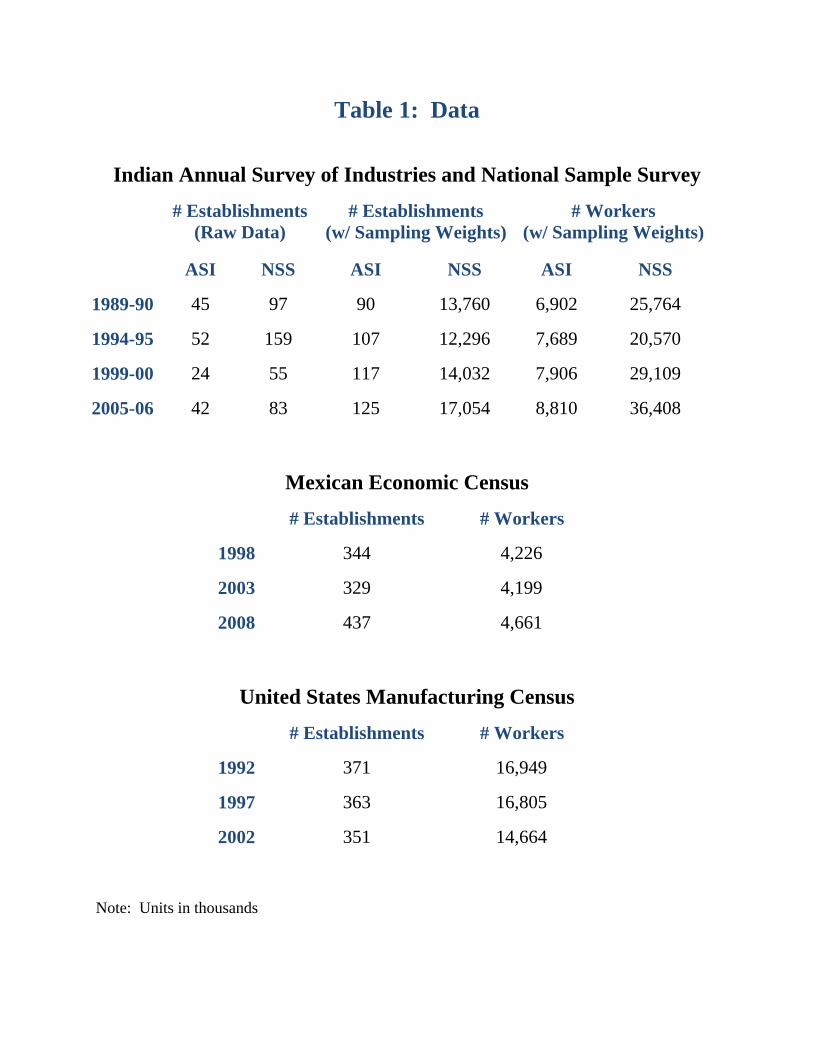
Table 1: Data
Indian Annual Survey of Industries and National Sample Survey
# Establishments (Raw Data)
# Establishments (w/ Sampling Weights)
# Workers (w/ Sampling Weights)
ASI NSS ASI NSS ASI NSS
1989-90 45 97 90 13,760 6,902 25,764
1994-95 52 159 107 12,296 7,689 20,570
1999-00 24 55 117 14,032 7,906 29,109
2005-06 42 83 125 17,054 8,810 36,408
Mexican Economic Census
# Establishments # Workers
1998 344 4,226
2003 329 4,199
2008 437 4,661
United States Manufacturing Census
# Establishments # Workers
1992 371 16,949
1997 363 16,805
2002 351 14,664
Note: Units in thousands
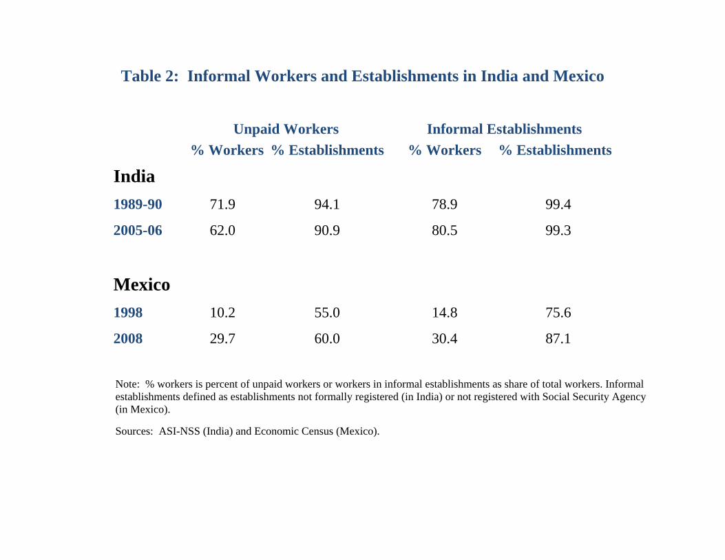
Table 2: Informal Workers and Establishments in India and Mexico
Unpaid Workers Informal Establishments
% Workers % Establishments % Workers % Establishments
India
1989-90 71.9 94.1 78.9 99.4
2005-06 62.0 90.9 80.5 99.3
Mexico
1998 10.2 55.0 14.8 75.6
2008 29.7 60.0 30.4 87.1
Note: % workers is percent of unpaid workers or workers in informal establishments as share of total workers. Informal establishments defined as establishments not formally registered (in India) or not registered with Social Security Agency (in Mexico).
Sources: ASI-NSS (India) and Economic Census (Mexico).

Table 3: Parameter Values
Parameter Definition Value or Target
Elasticity of substitution between varieties 3 for all models
ef Entry costs (in terms of labor) Average workers per plant in the U.S.
eg Growth of mean of entrant ln(TFPQ) 2.1% per year for all models (U.S. average TFP growth)
,a iA TFPQ across and within age groups Matches growth for each 5 year age cohort in the U.S. or India
,a i Exit by age, TFPQ Matches average rate for each 5 year age cohort in the U.S.;
slope with respect to ln(TFPQ) in the U.S. (‐0.0225)
,a i Tax rate on revenue by age, TFPQ Matches average ln(TFPR) in 5 year cohorts in the U.S. or India;
slope of ln(TFPR) wrt ln(TFPQ) in the U.S. (0.13) or India (0.56)
e S.D. of entrant ln(TFPQ) 1.01 (when not zero) to match U.S. entrant TFPQ dispersion
h Level parameter in the R&D cost function Set with b to match average U.S. TFPQ growth from age 0 to 30
b Convexity parameter in the R&D cost function Set to 100 to roughly match average Indian TFPQ growth by age
Coefficient of relative risk aversion 2 for all models
Discount rate Always 0.8% per year to arrive at a real interest rate of 5%
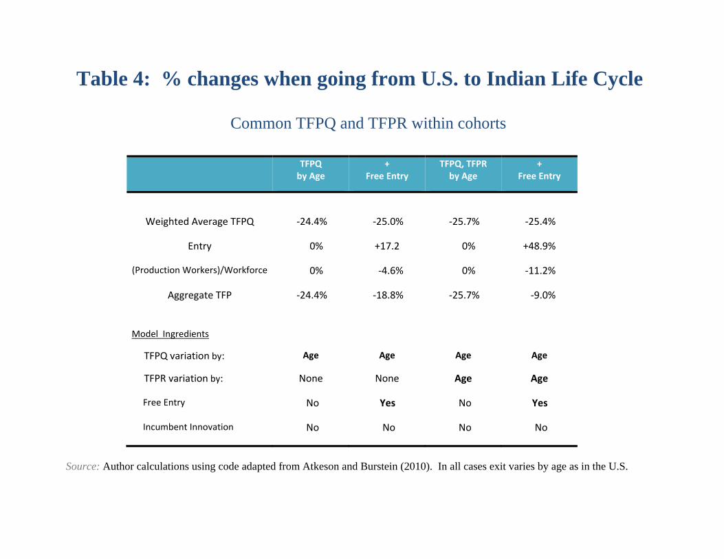
Table 4: % changes when going from U.S. to Indian Life Cycle
Common TFPQ and TFPR within cohorts
TFPQ by Age
+ Free Entry
TFPQ, TFPR by Age
+ Free Entry
Weighted Average TFPQ ‐24.4% ‐25.0% ‐25.7% ‐25.4%
Entry 0% +17.2 0% +48.9%
(Production Workers)/Workforce 0% ‐4.6% 0% ‐11.2%
Aggregate TFP ‐24.4% ‐18.8% ‐25.7% ‐9.0%
Model Ingredients
TFPQ variation by: Age Age Age Age
TFPR variation by: None None Age Age
Free Entry No Yes No Yes
Incumbent Innovation No No No No
Source: Author calculations using code adapted from Atkeson and Burstein (2010). In all cases exit varies by age as in the U.S.

Table 5: % changes when going from U.S. to Indian Life Cycle
Dispersion in TFPQ and TFPR within cohorts
Fixed Entry Free Entry
Endogenous Entrant Quality
Incumbent Innovation
Weighted Average TFPQ ‐54.5% ‐54.5% ‐64.6% ‐55.7%
Entry 0% +49.3% +62.1% +73.9%
(Production Workers)/Workforce 0% ‐12.3% ‐0.0% ‐9.4%
Aggregate TFP ‐54.5% ‐51.2% ‐54.9% ‐47.1%
Model Ingredients
TFPQ, TFPR variation by: Age, Within Age, Within Age, Within Age, Within
Free Entry No Yes Yes Yes
Endogenous Entrant Quality No No Yes No
Incumbent Innovation No No No Yes
Source: Author calculations using code adapted from Atkeson and Burstein (2010). Exit varies by both age and TFPQ as in the U.S.
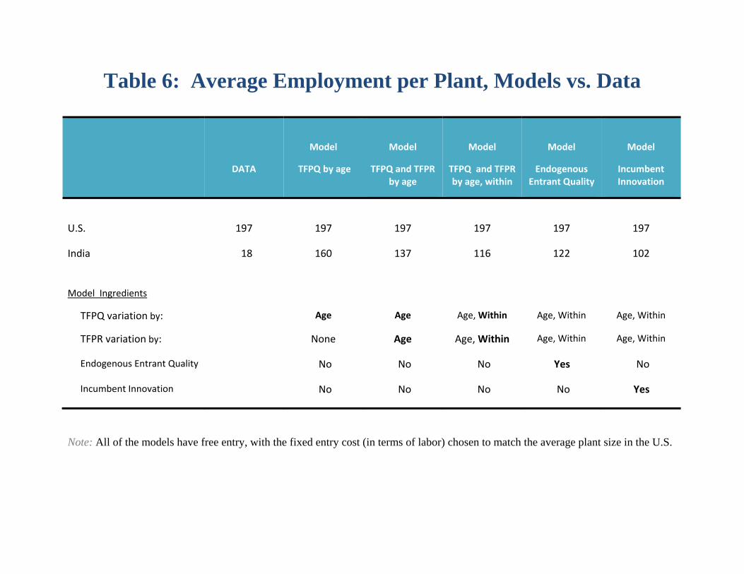
Table 6: Average Employment per Plant, Models vs. Data
DATA
Model
TFPQ by age
Model
TFPQ and TFPR by age
Model
TFPQ and TFPR by age, within
Model
Endogenous Entrant Quality
Model
Incumbent Innovation
U.S. 197 197 197 197 197 197
India 18 160 137 116 122 102
Model Ingredients
TFPQ variation by: Age Age Age, Within Age, Within Age, Within
TFPR variation by: None Age Age, Within Age, Within Age, Within
Endogenous Entrant Quality No No No Yes No
Incumbent Innovation No No No No Yes
Note: All of the models have free entry, with the fixed entry cost (in terms of labor) chosen to match the average plant size in the U.S.
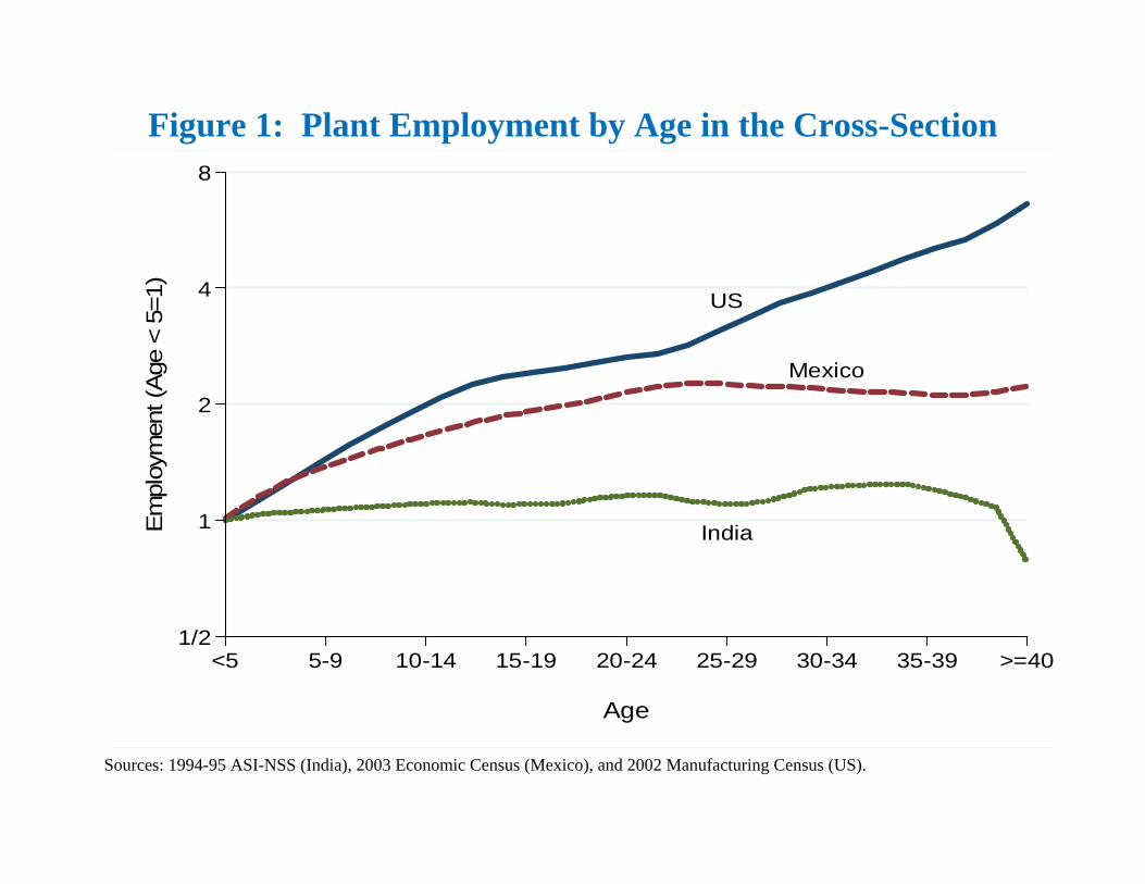
Figure 1: Plant Employment by Age in the Cross-Section
US
Mexico
India
1/2
1
2
4
8E
mplo
ymen
t (A
ge <
5=1)
<5 5-9 10-14 15-19 20-24 25-29 30-34 35-39 >=40
Age
Sources: 1994-95 ASI-NSS (India), 2003 Economic Census (Mexico), and 2002 Manufacturing Census (US).
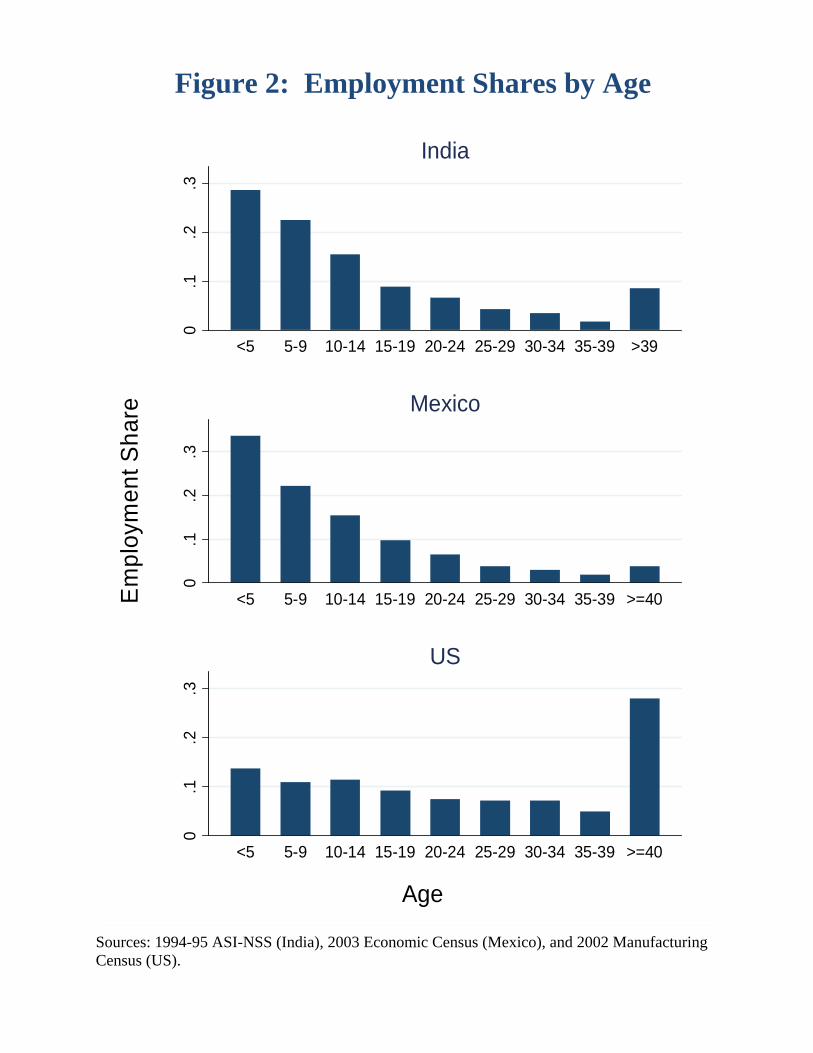
Figure 2: Employment Shares by Age
0.1
.2.3
<5 5-9 10-14 15-19 20-24 25-29 30-34 35-39 >39
India
0.1
.2.3
<5 5-9 10-14 15-19 20-24 25-29 30-34 35-39 >=40
Mexico
0.1
.2.3
<5 5-9 10-14 15-19 20-24 25-29 30-34 35-39 >=40
US
Em
plo
ymen
t Sh
are
Age
Sources: 1994-95 ASI-NSS (India), 2003 Economic Census (Mexico), and 2002 Manufacturing Census (US).

Figure 3: Employment Growth over the Life-Cycle
US
Mexico
India
1/4
1/2
1
2
4
8
16
Em
plo
ymen
t (A
ge <
5=1)
<5 5-9 10-14 15-19 20-24 25-29 30-34 >=35
Age
Notes: Employment growth with age imputed from 1992 and 1997 US Manufacturing Census, 1998 and 2003 Mexican Economic Census, and 1989-90 and 1994-95 Indian ASI-NSS.
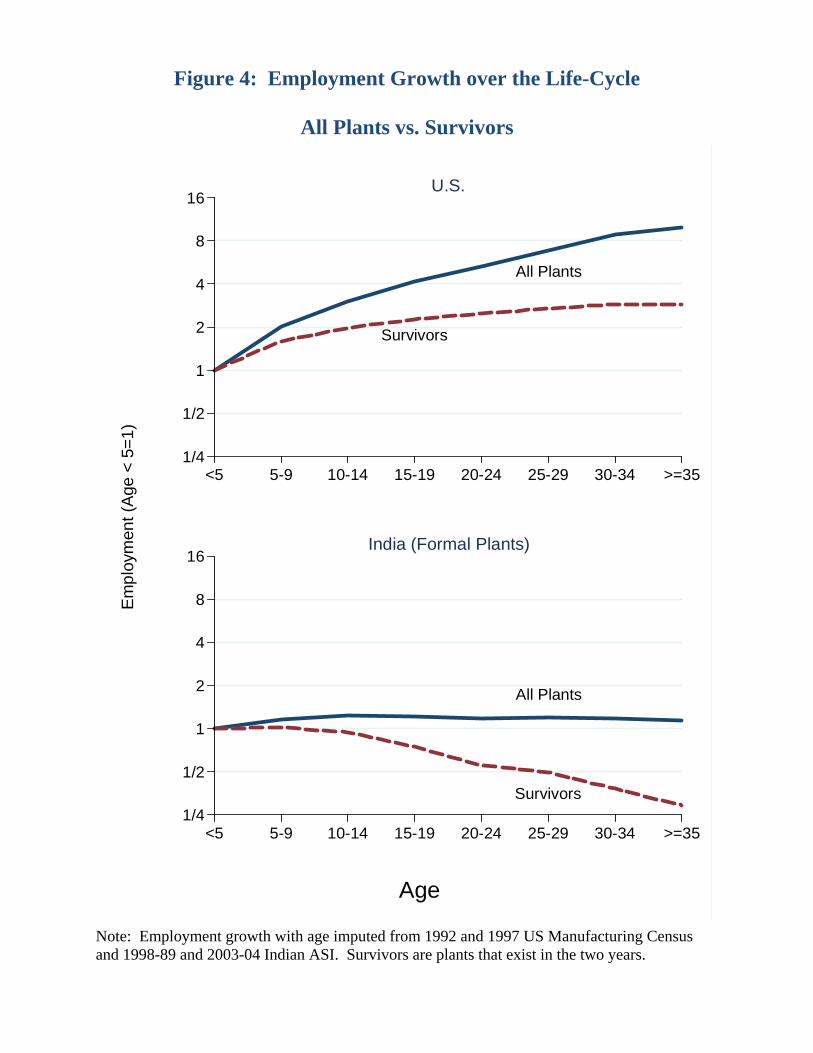
Figure 4: Employment Growth over the Life-Cycle
All Plants vs. Survivors
Survivors
All Plants
1/4
1/2
1
2
4
8
16
<5 5-9 10-14 15-19 20-24 25-29 30-34 >=35
U.S.
Survivors
All Plants
1/4
1/2
1
2
4
8
16
<5 5-9 10-14 15-19 20-24 25-29 30-34 >=35
India (Formal Plants)
Em
plo
ymen
t (A
ge <
5=
1)
Age
Note: Employment growth with age imputed from 1992 and 1997 US Manufacturing Census and 1998-89 and 2003-04 Indian ASI. Survivors are plants that exist in the two years.
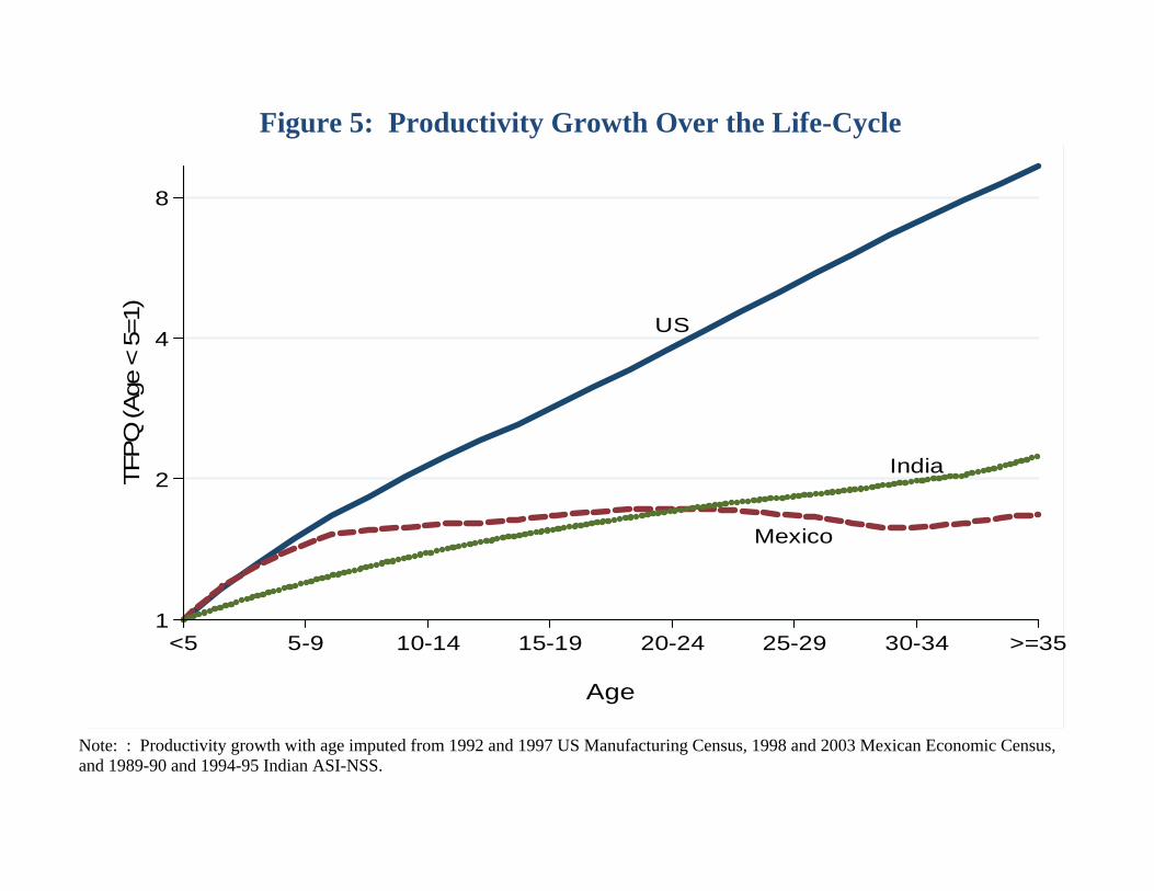
Figure 5: Productivity Growth Over the Life-Cycle
US
India
Mexico
1
2
4
8
TFP
Q (Age
< 5
=1)
<5 5-9 10-14 15-19 20-24 25-29 30-34 >=35
Age
Note: : Productivity growth with age imputed from 1992 and 1997 US Manufacturing Census, 1998 and 2003 Mexican Economic Census, and 1989-90 and 1994-95 Indian ASI-NSS.
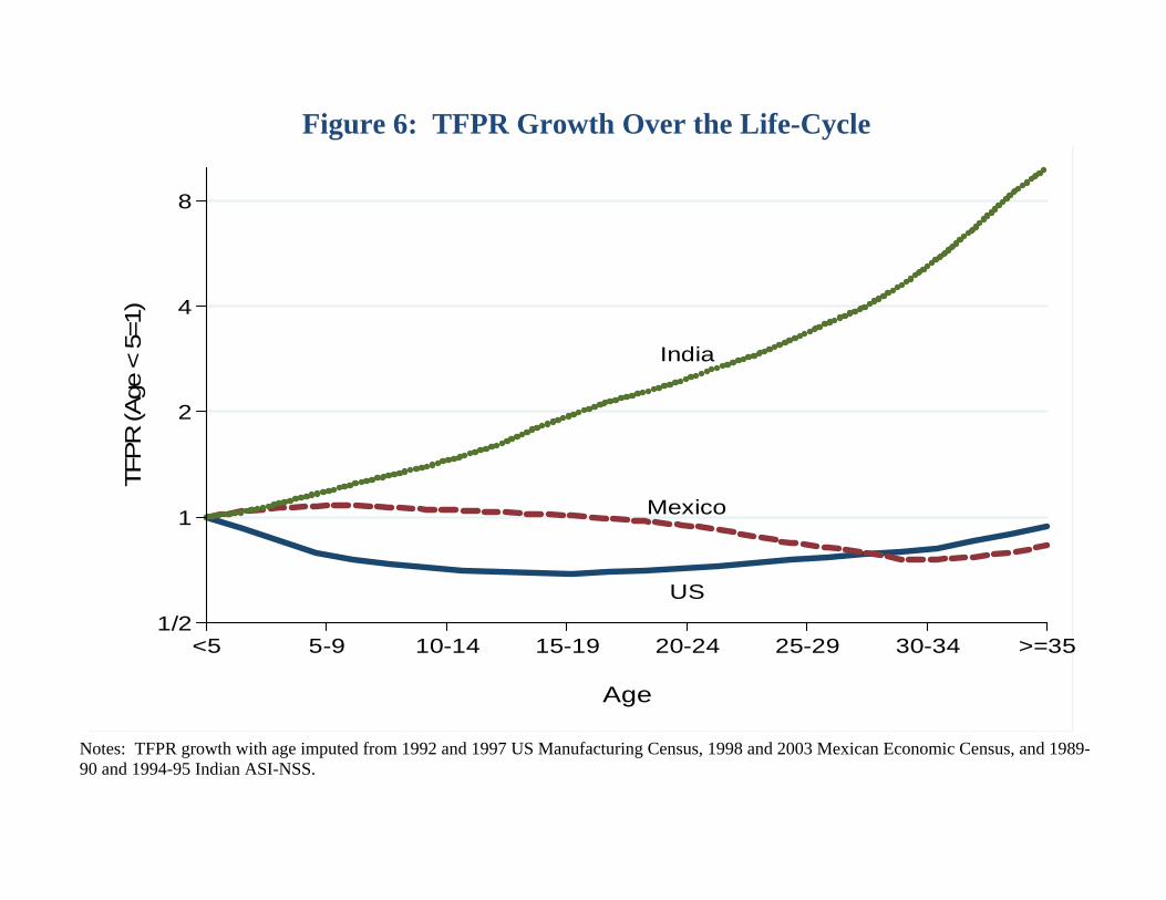
Figure 6: TFPR Growth Over the Life-Cycle
US
Mexico
India
1/2
1
2
4
8
TFPR
(Age
< 5
=1)
<5 5-9 10-14 15-19 20-24 25-29 30-34 >=35
Age
Notes: TFPR growth with age imputed from 1992 and 1997 US Manufacturing Census, 1998 and 2003 Mexican Economic Census, and 1989-90 and 1994-95 Indian ASI-NSS.
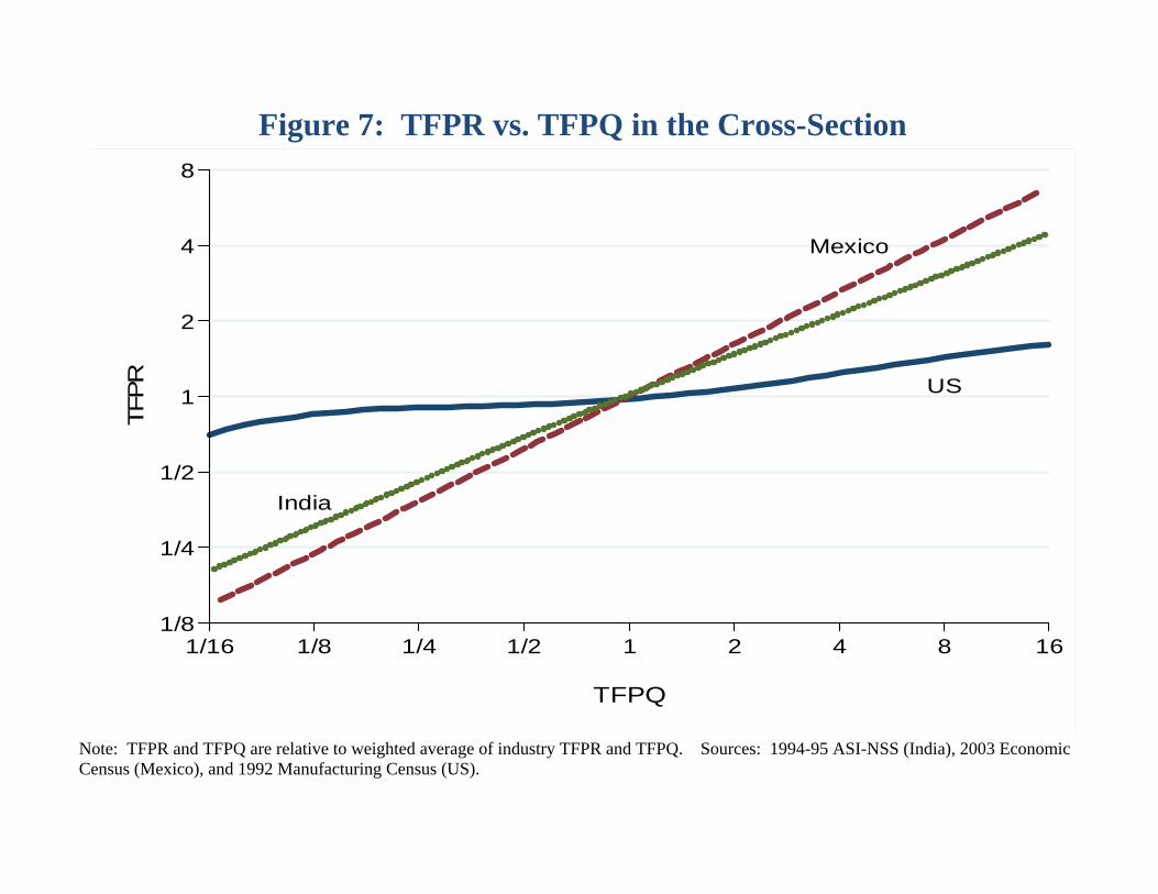
Figure 7: TFPR vs. TFPQ in the Cross-Section
US
Mexico
India
1/8
1/4
1/2
1
2
4
8
TFPR
1/16 1/8 1/4 1/2 1 2 4 8 16
TFPQ
Note: TFPR and TFPQ are relative to weighted average of industry TFPR and TFPQ. Sources: 1994-95 ASI-NSS (India), 2003 Economic Census (Mexico), and 1992 Manufacturing Census (US).
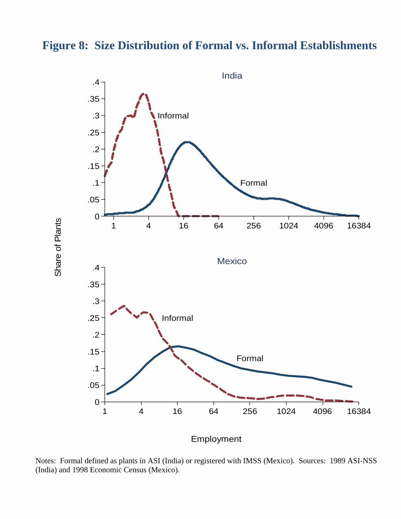
Figure 8: Size Distribution of Formal vs. Informal Establishments
Formal
Informal
0
.05
.1
.15
.2
.25
.3
.35
.4
1 4 16 64 256 1024 4096 16384
India
Formal
Informal
0
.05
.1
.15
.2
.25
.3
.35
.4
1 4 16 64 256 1024 4096 16384
Mexico
Sha
re o
f Pla
nts
Employment
Notes: Formal defined as plants in ASI (India) or registered with IMSS (Mexico). Sources: 1989 ASI-NSS (India) and 1998 Economic Census (Mexico).
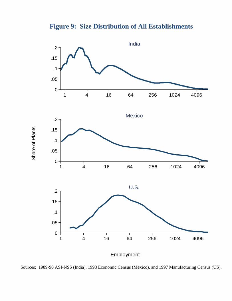
Figure 9: Size Distribution of All Establishments
0
.05
.1
.15
.2
1 4 16 64 256 1024 4096
India
0
.05
.1
.15
.2
1 4 16 64 256 1024 4096
Mexico
0
.05
.1
.15
.2
1 4 16 64 256 1024 4096
U.S.
Sha
re o
f Pla
nts
Employment
Sources: 1989-90 ASI-NSS (India), 1998 Economic Census (Mexico), and 1997 Manufacturing Census (US).
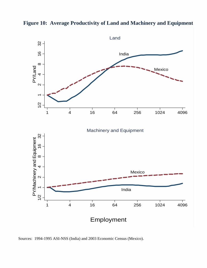
Figure 10: Average Productivity of Land and Machinery and Equipment
India
Mexico
1/2
12
48
16
32
PY
/Land
1 4 16 64 256 1024 4096
Land
Mexico
India
1/2
12
48
16
32
PY
/Mac
hin
ery
and
Equ
ipm
ent
1 4 16 64 256 1024 4096
Machinery and Equipment
Employment
Sources: 1994-1995 ASI-NSS (India) and 2003 Economic Census (Mexico).
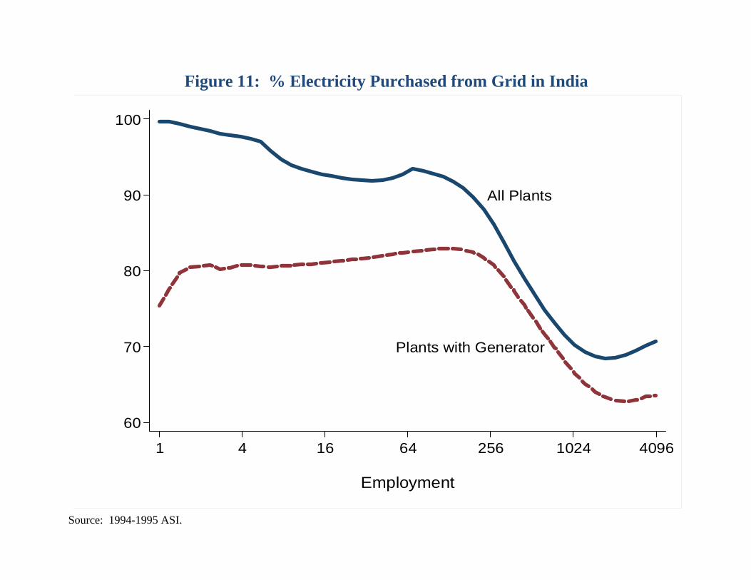
Figure 11: % Electricity Purchased from Grid in India
All Plants
Plants with Generator
60
70
80
90
100
1 4 16 64 256 1024 4096
Employment
Source: 1994-1995 ASI.
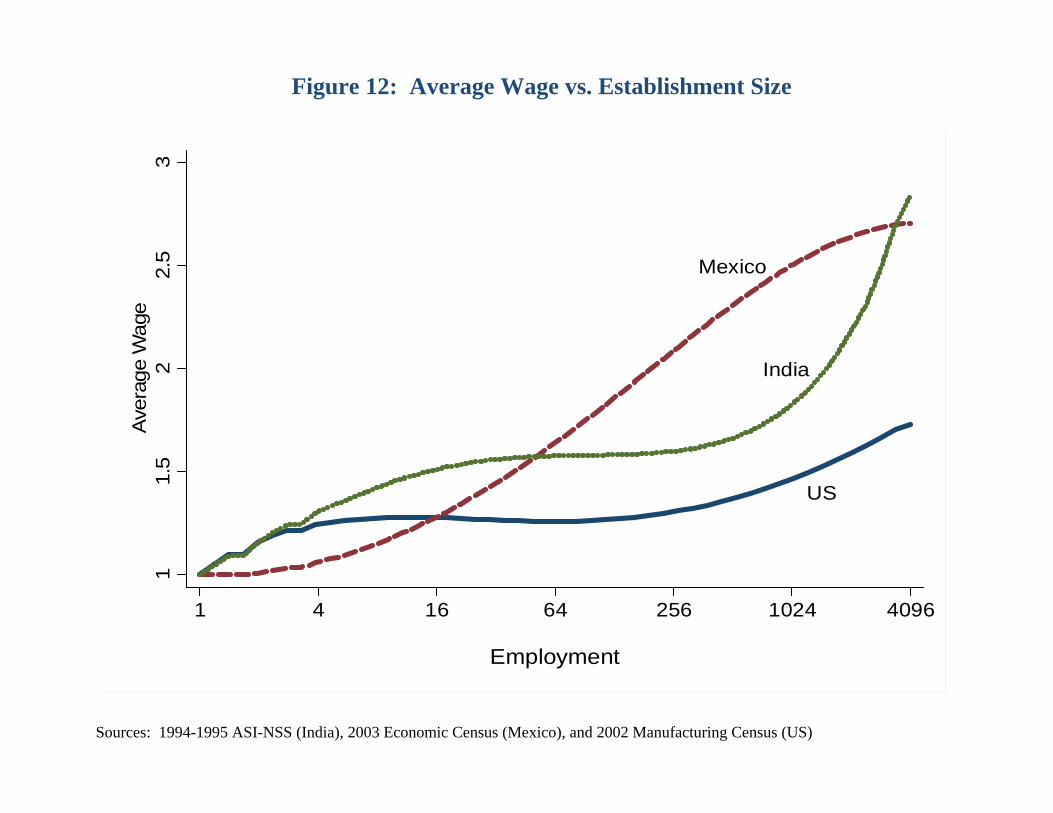
Figure 12: Average Wage vs. Establishment Size
Mexico
India
US
11.5
22.5
3A
vera
ge
Wage
1 4 16 64 256 1024 4096
Employment
Sources: 1994-1995 ASI-NSS (India), 2003 Economic Census (Mexico), and 2002 Manufacturing Census (US)
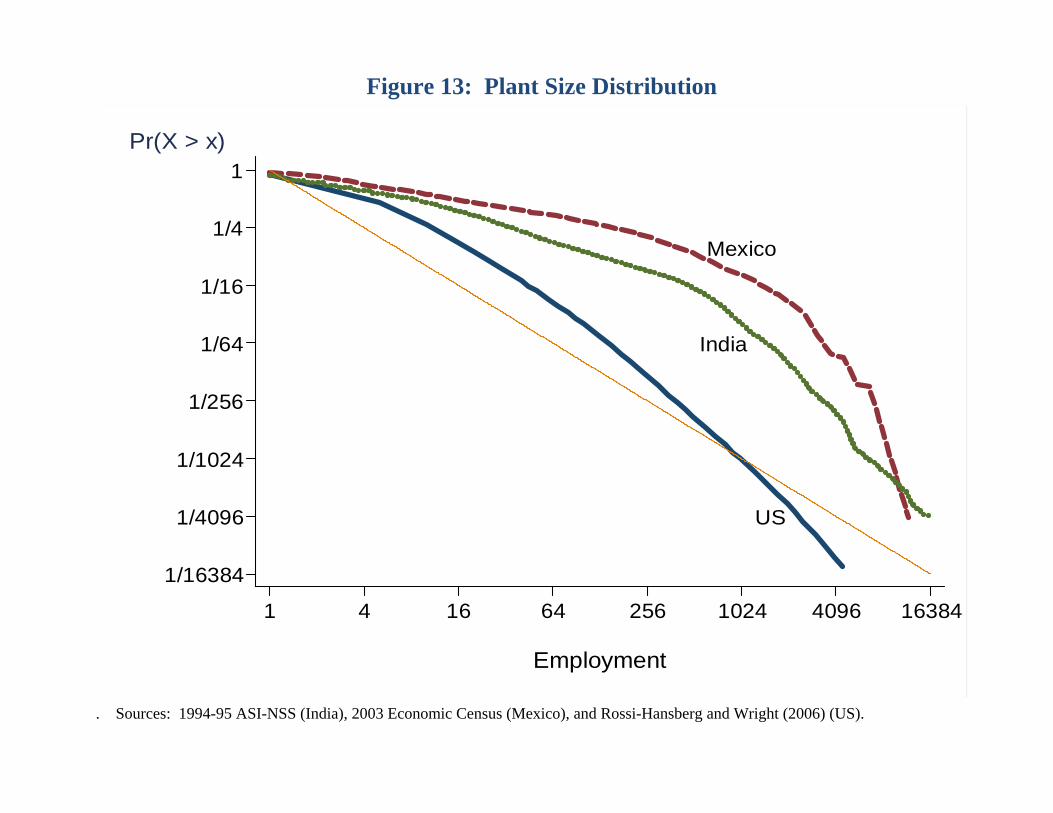
Figure 13: Plant Size Distribution
US
Mexico
India
1/16384
1/4096
1/1024
1/256
1/64
1/16
1/4
1
1 4 16 64 256 1024 4096 16384
Employment
Pr(X > x)
. Sources: 1994-95 ASI-NSS (India), 2003 Economic Census (Mexico), and Rossi-Hansberg and Wright (2006) (US).
25
References
Albuquerque, Rui and Hugo Hopenhayn (2004), "Optimal Lending Contracts and Firm Dynamics," Review of Economic Studies 71(2): 285-315. Arkolakis, Costas (2010), "Market Penetration Costs and the New Consumers Margin in International Trade," Journal of Political Economy 118 (June), 1151-1191. Atkeson, Andrew and Ariel Burstein (2010), “Innovation, Firm Dynamics, and International Trade,” Journal of Political Economy 118 (June), 1026-1053. Atkeson, Andrew G. and Patrick J. Kehoe (2005), “Modeling and Measuring Organizational Capital,” Journal of Political Economy 113 (October): 1026-1053. Besley, Timothy and Robin Burgess (2004), "Can Labor Regulations Hinder Economic Performance? Evidence from India," Quarterly Journal of Economics 119, 91-134. Bloom, Nicholas, Benn Eifert, David McKenzie, Aprajit Mahajan, and John Roberts (2011), “Does Management Matter: Evidence from India,” Stanford University. Buera, Francisco J., Joseph Kaboski, and Yongseok Shin (2011), “Finance and Development: A Tale of Two Sectors,” forthcoming in the American Economic Review. Cabral, Luis and Jose Mata (2003), "On the Evolution of the Firm Size Distribution: Facts and Theory," American Economic Review 93(4): 1075-90. Chaney, Thomas (2008), “Distorted Gravity: The Intensive and Extensive Margins of International Trade,” American Economic Review 98(4), 1707–1721. Clementi, Gian Luca and Hugo Hopenhayn (2006), "A Theory of Financing Constraints and Firm Dynamics," Quarterly Journal of Economics 121(1): 229-65. Cooley, Thomas and Vincenzo Quadrini (2001), "Financial Markets and Firm Dynamics," American Economic Review 91(5): 1286-1310. Davis, Steven, John Haltiwanger, and Scott Schuh (1996), Job Creation and Destruction. Cambridge, MA: MIT Press. Dunne, Timothy, Mark Roberts, and Larry Samuelson (1989), "The Growth and Failure of U.S. Manufacturing Plants," Quarterly Journal of Economics 104(4), 671-98. Ericson, Richard, and Ariel Pakes (1995), "Markov-Perfect Industry Dynamics: A Framework for Empirical Work," Review of Economic Studies 62(1): 53-82. Fattal Jaef, Roberto N. (2011), “Entry, Exit and Misallocation Frictions,” UCLA.
26
Foster, Lucia, John Haltiwanger, and Chad Syverson (2012), "The Slow Growth of New Plants: Learning about Demand?" University of Chicago mimeo. Gabaix, Xavier (1999), "Zipf's Law for Cities: An Explanation," Quarterly Journal of Economics 114(3): 739-767. Guner, Nezih, Gustavo Ventura, and Yi Xu (2008), “Macroeconomic Implications of Size- Dependent Policies,” Review of Economic Dynamics 11, 721–744. Holmes, Thomas and John Stevens (2012), "Exports, Borders, Distance, and Plant Size," Journal of International Economics, forthcoming. Hopenhayn, Hugo (1992), "Entry, Exit, and Firm Dynamics in Long Run Equilibrium," Econometrica 60(5): 1127-50. Hsieh, Chang-Tai and Peter J. Klenow (2009), “Misallocation and Manufacturing TFP in China and India,” Quarterly Journal of Economics 124 (4), 1403-1448. Levy, Santiago (2008), Good Intentions, Bad Outcomes, Washington, DC: Brookings Institution. Li, Nicholas (2011), “An Engel Curve for Variety,” University of California, Berkeley. Luttmer, Erzo (2007), "Selection, Growth, and the Size Distribution of Firms," Quarterly Journal of Economics 112 (3): 1103-1144. Midrigan, Virgiliu and Daniel Xu (2010), “Finance and Misallocation: Evidence from Plant-level Data,” Federal Reserve Bank of Minneapolis. Moll, Benjamin (2010), “Productivity Losses from Financial Frictions: Can Self-Financing Undo Capital Misallocation?”, Princeton University. Peters, Michael (2010), “Heterogeneous Mark-ups and Endogenous Misallocation”, MIT. Restuccia, Diego and Richard Rogerson (2008), “Policy Distortions and Aggregate Productivity with Heterogeneous Plants,” Review of Economic Dynamics 11, 707–720. Rossi-Hansberg, Esteban and Mark Wright (2007), "Establishment Size Dynamics in the Aggregate Economy," American Economic Review 97(5): 1639-1666. World Bank (2010), Doing Business 2011: Making a Difference for Entrepreneurs.