The International Association for the Properties of Water and Steam

Stockholm, Sweden July 2015

Guideline on the Fast Calculation of Steam and Water Properties with the Spline-Based Table Look-Up Method (SBTL)

2015 International Association for the Properties of Water and Steam Publication in whole or in part is allowed in all countries provided that attribution is given to the

International Association for the Properties of Water and Steam

Please cite as: International Association for the Properties of Water and Steam, Guideline on the Fast Calculation of Steam and Water Properties with the Spline-Based Table Look-Up Method (SBTL) (2015).

This Guideline has been authorized by the International Association for the Properties of Water and Steam (IAPWS) at its meeting in Stockholm, Sweden, 28 June – 03 July, 2015. The Members of IAPWS are: Britain and Ireland, Canada, the Czech Republic, Germany, Japan, Russia, Scandinavia (Denmark, Finland, Norway, Sweden), and the United States, plus Associate Members Argentina and Brazil, Australia, France, Greece, New Zealand, and Switzerland. The President at the time of adoption of this document was Dr. David Guzonas of Canada.

Summary The Spline-Based Table Look-Up Method (SBTL), described in this Guideline, is intended to be used for fast property calculations in extensive process simulations, such as Computational Fluid Dynamics (CFD), heat cycle calculations, simulations of non-stationary processes, and real-time process optimizations, where conventional multiparameter equations of state may be unsuitable because of their computing time consumption. Through the use of this method, the results of the underlying formulation (which may for example be IAPWS-IF97 or IAPWS-95) are accurately reproduced at high computational speed. The supporting document for this Guideline is an article by Kunick et al. [1].

This Guideline contains 68 pages, including this cover page.

Further information about this Guideline and other documents issued by IAPWS can be obtained from the Executive Secretary of IAPWS (Dr. R.B. Dooley, bdooley@structint.com) or from http://www.iapws.org.

IAPWS G13-15

2

Contents

1. List of Symbols and Nomenclature...................................................................................... 4 2. Introductory Remarks.......................................................................................................... 6 3. The Spline-Based Table Look-Up Method (SBTL)............................................................7

3.1. One-Dimensional Spline Functions.................................................................................7 3.1.1. Spline Functions...................................................................................................... 7

3.1.2. Transformations..................................................................................................... 10

3.1.3. Inverse Spline Functions........................................................................................11 3.1.4. Derivatives............................................................................................................. 12

3.2. Two-Dimensional Spline Functions.............................................................................. 13 3.2.1. Spline Functions.................................................................................................... 13 3.2.2. Transformations..................................................................................................... 17 3.2.3. Inverse Spline Functions........................................................................................19 3.2.4. Derivatives............................................................................................................. 21 3.2.5. Calculations in the Two-Phase Region.................................................................. 23

4. Spline Functions of (v,u) and Inverse Functions Based on IAPWS-IF97...................... 26 4.1. Range of Validity.......................................................................................................... 26 4.2. Spline Functions for the Single-Phase Region.............................................................. 27 4.3. Calculations in the Two-Phase Region......................................................................... 28 4.4. Derivatives..................................................................................................................... 28 4.5. Deviations from IAPWS-IF97....................................................................................... 28 4.6. Numerical Consistency at Region Boundaries.............................................................. 30 4.7. Computing-Time Comparisons..................................................................................... 31

5. Spline Functions of (p,h) and Inverse Functions Based on IAPWS-IF97...................... 33 5.1. Range of Validity.......................................................................................................... 33 5.2. Spline Functions for the Single-Phase Region.............................................................. 34 5.3. Calculations in the Two-Phase Region......................................................................... 34 5.4. Derivatives..................................................................................................................... 35 5.5. Deviations from IAPWS-IF97....................................................................................... 35 5.6. Numerical Consistency at Region Boundaries.............................................................. 37 5.7. Computing-Time Comparisons..................................................................................... 38

3

6. Spline Functions for the Metastable-Vapor Region Based on IAPWS-IF97................. 40 6.1.Spline Functions of (v,u)................................................................................................ 40

6.1.1. Deviations from IAPWS-IF97............................................................................... 40 6.1.2. Computing-Time Comparisons............................................................................. 42

6.2. Spline Functions of (p,h)............................................................................................... 42 6.2.1. Deviations from IAPWS-IF97............................................................................... 44 6.2.2. Computing-Time Comparisons............................................................................. 44

7. Spline Functions Based on IAPWS-95.............................................................................. 45 7.1. Spline Functions of (v,u)............................................................................................... 45

7.1.1. Range of Validity................................................................................................... 45 7.1.2. Spline Functions for the Single-Phase Regions..................................................... 46 7.1.3. Deviations from IAPWS-95.................................................................................. 46

7.2. Spline Functions of (p,h)............................................................................................... 48 7.2.1. Range of Validity................................................................................................... 48 7.2.2. Spline Functions for the Single-Phase Regions..................................................... 49 7.2.3. Deviations from IAPWS-95.................................................................................. 49

7.3. Computing-Time Comparisons..................................................................................... 49

8. Application of the SBTL Method in Computational Fluid Dynamics........................... 51 9. Application of the SBTL Method in Heat Cycle Calculation Software......................... 51 10. Generating Spline Functions for User-Specified Demands........................................... 51 11. References.......................................................................................................................... 52 APPENDIX.............................................................................................................................. 54

A1 Property Calculations in the Two-Phase Region from (p,h)...........................................54 A2 Property Calculations in the Two-Phase Region from (p,s)........................................... 54 A3 Property Calculations in the Two-Phase Region from (h,s)........................................... 54 A4 Property Calculations in the Two-Phase Region from (v,u)........................................... 55 A5 Property Calculations in the Two-Phase Region from (p,v)........................................... 57 A6 Property Calculations in the Two-Phase Region from (u,s)........................................... 57 A7 Transformations and Grid Dimensions...........................................................................59

4

1. List of Symbols and Nomenclature Symbol

a Spline polynomial coefficient f Function floor() Round down F Vector of functions h Specific enthalpy i Interval index in 1x direction (i) Node within the interval {i} {i} Interval K K

1, 1 1, 1+≤ <i ix x x (i, j) Node within the cell {i, j} {i, j} Cell defined by the intervals {i} and {j} I Number of nodes along 1x j Interval index in 2x direction {j} Interval K K

2, 2 2, 1+≤ <j jx x x J Number of nodes along 2x J Jacobian matrix p Pressure s Specific entropy T Absolute temperature TOL Tolerance for iterative procedures (typically less than or equal to 10−8) u Specific internal energy v Specific volume w Speed of sound x Vapor fraction

1x Independent variable

1x Transformed independent variable

2x Independent variable

2x Transformed independent variable X Vector of unknowns z Dependent variable z Transformed dependent variable η Dynamic viscosity

5

Superscript

AUX Auxiliary spline function G Spline function for the gas region HT Spline function for the high-temperature region INV Inverse spline function K Knot L Spline function for the liquid region MG Spline function for the metastable-vapor and the gas region SPL Spline function T Transposed

Subscript

i Interval index in 1x direction j Interval index in 2x direction min Minimum value max Maximum value perm Permissible value RMS Root-mean-square value of a quantity, see below s At saturation

The root-mean-square value is

2RMS

1

1 ( )=

∆ = ∆∑N

nn

x xN

,

where ∆xn can be either the absolute or percentage difference between the corresponding quantities x; N is the number of ∆xn values (depending on the property, between 10 million and 100 million points are uniformly distributed over the respective range of validity).

Definitions

Backward function Inverse function for 1( )x z , 1 2( , )x z x , or 2 1( , )x x z Forward function Explicit function for 1( )z x or 1 2( , )z x x Knot Connection point of neighboring spline polynomials Node Point to be intersected by a spline polynomial Spline function Continuous, piecewise-defined function consisting of several spline

polynomials Spline polynomial Polynomial whose coefficients are determined with a spline algorithm

6

2. Introductory Remarks In Computational Fluid Dynamics (CFD) and simulations of non-stationary processes, fast and

accurate algorithms for the calculation of thermodynamic and transport properties are often required. Fluid property functions and their first derivatives generally need to be continuous. Furthermore, forward and backward functions need to be numerically consistent with each other. In CFD, the independent variables of the required property functions are often the specific volume and the specific internal energy (v,u). Moreover, fluid properties are also calculated from pressure and specific volume (p,v) or specific internal energy and specific entropy (u,s). These functions need to be calculated by iteration from the underlying property formulation, which might be the IAPWS Industrial Formulation 1997 (IAPWS-IF97) [2, 3] or the IAPWS Formulation 1995 for General and Scientific Use (IAPWS-95) [4, 5]. This is computationally intensive, and therefore inappropriate for CFD. Backward equations, enabling calculations from alternative variable combinations, are available for IAPWS-IF97 for some functions, but not for functions of (v,u), (p,v), and (u,s).

The simulation of non-stationary processes in heat cycles often requires property calculations from pressure and specific enthalpy (p,h), pressure and specific entropy (p,s), and specific enthalpy and specific entropy (h,s). In order to avoid iterative procedures and to reduce the computing time, the industrial formulation IAPWS-IF97 and its supplementary releases [6, 7, 8, 9] contain backward equations for several pairs of variables, such as (p,h), (p,s), and (h,s). Due to the imperfect numerical consistency with the basic equations of IAPWS-IF97, the application of backward equations for simulating non-stationary processes can lead to convergence problems. In these situations, backward functions should be calculated by iteration from the basic equations with starting values determined from the available backward equations.

For fast property calculations from various inputs, IAPWS adopted the “Guideline on the Tabular Taylor Series Expansion Method for Calculation of Thermodynamic Properties of Water and Steam Applied to IAPWS-95 as an Example (TTSE)” [10] in 2003. The TTSE method is very fast, but adjacent Taylor series are not connected continuously. This characteristic leads to numerical problems in CFD and non-stationary simulations with very small spatial and time discretization.

In order to provide an alternative method for fast and numerically consistent property calculations in extensive numerical process simulations, the Spline-Based Table Look-Up method (SBTL) [1, 11] has been developed. This method is intended to be a supplement to existing property formulations, such as IAPWS-IF97 [2] and IAPWS-95 [4]. The use of the SBTL method results in good agreement with these and other standards, but with significantly reduced computing time. Additionally, with the SBTL method, backward functions are calculated with complete numerical consistency with their corresponding forward functions, e.g., the formulations for u(p,v) and p(v,u) are mathematically self-consistent.

This Guideline describes the fundamentals of the SBTL method and its application to the IAPWS-IF97 and IAPWS-95 formulations. It details computing-time comparisons between property functions calculated from IAPWS-IF97 and IAPWS-95 and the SBTL method. The advantage in computing speed in practical CFD and heat-cycle simulations has been evaluated. The results of these investigations are given in this document.

7

3. The Spline-Based Table Look-Up Method (SBTL)

The Spline-Based Table Look-Up method (SBTL) applies polynomial spline interpolation techniques to approximate the results of existing equations of state, with high accuracy and low computing time. The accuracy, computing time, and memory storage advantages are enabled with specialized coordinate transformations and simplified search algorithms as described below. The properties in the single-phase regions, such as T(p,h), are represented by two-dimensional spline functions in the common form SPL

1 2( , )z x x , whereas the phase boundaries, such as s ( )T p , are represented by one-dimensional spline functions SPL

1( )z x . Algorithms for calculating properties in the two-phase region that are consistent with the single-phase properties are also provided.

In this document, and in [1], the basic principles of the SBTL method are outlined. A more detailed description is given in the publication by Kunick [11].

3.1. One-Dimensional Spline Functions

3.1.1. Spline Functions A one-dimensional polynomial spline function SPL

1( )z x is a continuous, piecewise-defined function consisting of several spline polynomials. The spline function interpolates values between a series of discrete data points, the so-called nodes (see Fig. 1). The number I and the location 1,ix of the nodes are chosen to ensure the desired accuracy. The 1,( )i iz x values of the nodes are calculated from the underlying function 1( )z x . The spline polynomials are connected at knots, which can either be equal or unequal to the nodes. For the SBTL method, the knots are located at the midpoint between the nodes along 1x , which results in symmetric boundary conditions leading to superior accuracy [12]. A spline polynomial ranges over the interval {i} between two knots and intersects the node (i) within. The z positions of the knots result from the spline algorithm as explained below.

In most numerical process simulations, fluid property functions need to be continuously differentiable once. The quadratic spline function is the simplest approach to continuously represent a one-dimensional function and its first derivative. Furthermore, the quadratic spline polynomial can easily be inverted. This enables the calculation of numerically consistent backward functions, which are the so-called inverse spline functions. Therefore, in this document the calculation of properties with the SBTL method is carried out through the use of quadratic spline polynomials, as opposed to higher order polynomials, to create a spline function SPL

1( )z x from the underlying function 1( )z x .

In order to increase the accuracy of the spline function, both the independent variable 1x and the dependent variable z are transformed into 1x and z , respectively, so that the transformed spline function yields SPL

1( )z x . A description of the transformations for one-dimensional spline functions can be found in Sec. 3.1.2. More detailed information on this subject is given in [11].

8

The spline function is created in transformed coordinates through the use of quadratic spline polynomials

{ } ( ) ( )3 1

1 1 1,1

−

== −∑ k

ik iik

z x a x x , (1.1)

where 1x is the transformed independent variable and z is the transformed dependent variable in the interval {i}. In Eq. (1.1), 1,ix is the transformed value of the independent variable at the node (i), and ika are the three coefficients of the quadratic spline polynomial valid in the interval {i}. Eq. (1.1) can also be written as

{ } ( ) 21 1 2 1, 3 1,= + ∆ + ∆i i i i iiz x a a x a x (1.2)

with ( )1, 1 1,∆ = −i ix x x . (1.3)

The I polynomials are connected at knots aligned as shown in Fig. 1, where I denotes the number of nodes along 1x . Each polynomial { } ( )1iz x is used in an interval {i} and intersects the node (i) at 1,( )i iz x .

Figure 1: Series of nodes and series of knots with interval {i} and spline polynomial { } ( )1iz x .

The K

1,ix values of the I+1 knots are located at the midpoint between the nodes along 1x , so that

( )K1, 1 1, 1, 1

12+ += +i i ix x x , 1, ... , 1= −i I (1.4)

K1, 1+ix

( )Node i

iz

1x

1,∆ ix1x

z

1,ixK

1,ixK1∆x

{ } ( )1Spline polynomial iz x

K1,1x

( )1z x

Interval{ }i

Knot i

KnotNode

( )SPL1z x

{ } ( )1iz x

{ }in the interval i

9

( )K1,1 1,1 1,2 1,1

12

= − −x x x x , and ( )K1, 1 1, 1, 1, 1

12+ −= + −I I I Ix x x x . (1.5, 1.6)

The number of nodes I is chosen to ensure the required accuracy of the spline function over its full domain of definition ( ) ( )1,1 1 1,min 1, 1 1,max, = = Ix x x x x x . The nodes are distributed equidistantly along 1x so that a simple search algorithm can be used to determine the interval {i} in the series of knots that fulfills K K

1, 1 1, 1+≤ <i ix x x for a given transformed variable 1x . For equidistant nodes, and therefore equidistant knots, i can easily be calculated from

K1 1,1

K1

floor − = ∆

x xi

x . (1.7)

The distribution of nodes and knots can also be manipulated by piecewise equidistant nodes, in ranges for which 1 1, 1 1,+∆ = −i ix x x is constant. Furthermore, the node spacing along 1x depends on the transformation ( )1 1x x . Basic principles of transformation techniques are outlined in Sec. 3.1.2 and described in more detail in [11].

The 3I coefficients ika of the I spline polynomials are obtained from the following conditions. Each of the I polynomials { } ( )1iz x must intersect the node (i)

{ } ( ) ( )1, 1,=i i iiz x z x 1, ... , =i I . (1.8)

Furthermore, the z values at the inner I−1 knots have to be equal for the adjacent polynomials

{ } ( ) { } ( )K K1, 1 1, 11+ ++=i ii iz x z x 1, ... , 1= −i I . (1.9)

The derivative ( )d dz x at each of these knots must also be equal

{ }( )

{ }( )K K

1, 1 1, 11 1 1

d dd d+ +

+

=i ii i

z zx xx x

1, ... , 1= −i I . (1.10)

At the outer knots, these derivatives are to be calculated from the underlying function ( )1z x with

{ }( ) ( )K K

1,1 1,11 11

d dd d=

=i

z zx xx x

and { }

( ) ( )K K1, 1 1, 1

1 1

d dd d+ +

=

=I Ii I

z zx xx x

, (1.11, 1.12)

where 1

1 1 1

dd d dd d d d

=xz z z

x z x x.

The linear system of Eqs. (1.8 - 1.12) is solved in order to obtain the 3I coefficients ika of the spline polynomials. This ensures continuous behavior of the spline function and its first derivatives at the knots. A comprehensive solution of the mathematical problem is given in [12]. Once all the coefficients ika are determined, they are stored together with the values of the nodes and knots in a look-up table.

In order to calculate SPL1( )z x , the variable 1x is first transformed into 1x with the

transformation function 1 1( )x x . From Eq. (1.7), the index i of the interval is then determined.

10

Finally, the transformed variable z is calculated from the spline polynomial { } 1( )iz x , Eq. (1.1), and converted to z with the inverse transformation function ( )z z .

3.1.2. Transformations In order to increase the accuracy of a quadratic spline function, the coordinates are transformed

in such a way that the third derivative, i.e., the change in curvature, is reduced. Both the independent variable 1x and the dependent variable z can be transformed with functions of the form 1 1( )x x and ( )z z . If ( )z z is nearly proportional to 1 1( )x x , then the change in curvature of the transformed function 1( )z x is smaller than that of 1( )z x .

The transformation functions are continuous and monotonic. An analytic solution for the inverse transformation function ( )z z is provided. For the inverse spline function INV

1 ( )x z , the inverse transformation function 1 1( )x x should also be analytical.

Figure 2: Untransformed function 1( )z x with nodes equidistant in 1x , rather than in 1x .

Figure 3: Transformed function 1( )z x with nodes equidistant in 1x .

The effect of variable transformations is illustrated in Figs. 2 and 3. The untransformed function, see Fig. 2, exhibits a non-zero third derivative, which cannot be described with a quadratic function. If, for instance, z is nearly proportional to 1 1( )x x , see Fig. 3, the accuracy of the interpolation between the nodes increases because the spline polynomial can better reproduce the transformed function. In many cases, several alternatives of analogous transformations of z and

1x are feasible. Due to more suitable node distributions, the transformation of 1x into 1x is usually superior to the transformation of z. Another useful approach to efficiently reduce the change in curvature is a transformation of the form 1( , )z z x . If required, the accuracy and computing time of

Node

1∆x1∆x 1∆x1∆x

z

( )1z x

1∆x1x

1∆x1,1x 1,Ix

( )1z x Nodez

1x1,Ix1,1x

11

the spline function itself, and its inverse spline function, must be assessed for the different transformation approaches to determine the tradeoff between these criteria.

The concepts explained above offer several alternatives to create a spline function, and can be combined. Considering the requirements for accuracy, computing speed, range of validity, and memory consumption, different transformation techniques must be assessed and the most suitable variant must be chosen. More details on variable transformations are given in [11].

3.1.3. Inverse Spline Functions From the spline function ( )SPL

1z x , the inverse spline function INV1 ( )x z can be calculated with

complete numerical consistency. The transformed variable 1x is obtained by inverting the polynomial { } ( )1iz x , Eq. (1.1), in the interval {i}, which results in

{ } ( )( )( )2

INV1,1,

4

2

− ± −= +

i i i iii

i

B B A C zx z x

A (1.13)

with 3=i iA a ,

2=i iB a , and ( ) 1= −i iC z a z .

For a monotonic spline polynomial { } ( )1iz x in the interval {i}, the sign (±) in Eq. (1.13) is negative if ( ) 2 2

1 1sgn( ) d d (d d ) 0⋅ ⋅ <iA z x z x , otherwise it is positive. The inequality yields 0<iB . Therefore, the sign (±) in Eq. (1.13) equals sgn( )iB if the spline polynomial is monotonic

in the interval {i}.

In order to determine the interval index i from Eq. (1.7) along 1x for a given z , an auxiliary spline function AUX

1 ( )x z is used to calculate an estimate for 1x .

The procedure for calculating 1( )x z is as follows. First, the variable z is transformed into z . The index i of the interval that belongs to z is determined with the auxiliary spline function

( )AUX1x z and Eq. (1.7). The inverse spline polynomial { } ( )INV

1, ix z , Eq. (1.13), is then evaluated. The result must fulfill the condition K K

1, 1 1, 1+≤ ≤i ix x x ; otherwise, the index i needs to be incremented or decremented, and the calculation repeated. Eventually, 1x is converted to 1x with the inverse transformation function 1 1( )x x .

Non-monotonic functions have two valid solutions in the interval {i} where the extremum of ( )SPL

1z x is located. This extremum is calculated from

{ } 1,1,ˆ

2= − +i

iii

Bx xA

and { } { }( ) { }( )23 1, 2 1, 11, 1,

ˆ ˆˆ = ⋅ − + ⋅ − +i i i i ii i iz a x x a x x a . (1.14, 1.15)

12

The coefficients of the auxiliary spline polynomial are stored together with the coefficients of the original spline polynomial along with values of nodes and knots in the look-up table. This table, and the associated algorithm for calculating the inverse spline function, is written to a source code file for application in computer programs (see Sec. 10).

A comprehensive description of the calculation of the inverse spline functions is given in [11].

3.1.4. Derivatives The first derivative of the spline function SPL

1( )z x with respect to the independent variable 1x is calculated analytically from

{ } { }

1

1

1 1 1

d d dd d d

∂ = ⋅ ⋅ ∂

i i

x

z z xzx x z x

, (1.16)

where the derivative of the spline function with the transformed variables, Eq. (1.1), within interval { }i is calculated from

{ }2 3 1,

1

d2

d

= + ∆

ii i i

za a x

x. (1.17)

The derivative of the general transformation function 1( , )z z x is simplified to

1

dd

∂ = ∂ x

z zz z

(1.18)

if the transformation of z is independent of 1x , i.e., ( )=z z z .

13

3.2. Two-Dimensional Spline Functions

3.2.1. Spline Functions A two-dimensional polynomial spline function SPL

1 2( , )z x x is a continuous, piecewise-defined function consisting of several spline polynomials. The spline function interpolates values between a set of discrete data points, the so-called grid of nodes (see Fig. 4). The number of nodes IJ and their ( )1, 2,,i jx x locations are chosen to ensure the desired accuracy. The 1, 2,( , )ij i jz x x values of the nodes are calculated from the underlying function 1 2( , )z x x . The spline polynomials are connected at knots, which can either be equal or unequal to the nodes. For the SBTL method, the knots are located at the midpoint between the nodes along 1x and 2x respectively, which results in symmetric boundary conditions leading to superior accuracy [13]. A spline polynomial ranges over a rectangular cell {i,j} between four knots and intersects the node within. The z positions of the knots result from the spline algorithm as explained below.

In most numerical process simulations, fluid property functions need to be continuously differentiable once. The bi-quadratic spline polynomial is the simplest approach that is capable of fulfilling this requirement. Furthermore, the bi-quadratic spline polynomial can easily be inverted. This enables the calculation of numerically consistent backward functions, the so-called inverse spline functions. Therefore, in this document the SBTL method is carried out through the use of bi-quadratic spline polynomials as opposed to higher order polynomials to create a spline function

SPL1 2( , )z x x from the underlying function 1 2( , )z x x .

In order to increase the accuracy of the spline function, both the independent variables 1x and 2x , as well as the dependent variable z, are transformed into 1x , 2x , and z so that the transformed

spline function yields SPL1 2( , )z x x . The bi-quadratic spline interpolation across rectangular cells

with continuous first derivatives requires a rectangular grid of nodes in the 1 2( , )x x projection. Through the use of transformations, the irregularly shaped domain of validity of a function can be transformed into a rectangle, and the distribution of nodes can be controlled more effectively. Alternatively, the function 1 2( , )z x x must be extrapolated. A description of the transformations for two-dimensional spline functions can be found in Sec. 3.2.2. More detailed information on this subject is given in [11].

The spline function is created in transformed coordinates through the use of bi-quadratic spline polynomials

{ } ( ) ( ) ( )3 3 11

1 2 1 1, 2 2,,1 1

,−−

= == − −∑∑

lkijkl i ji j

k lz x x a x x x x , (2.1)

where 1x and 2x represent the transformed independent variables, { },i jz is the transformed dependent variable in the cell {i,j}, 1,ix and 2, jx are the transformed values of the independent variables at the node (i,j), and ijkla are the nine coefficients of the spline polynomial valid in the cell {i,j}. Equation (2.1) can also be written as

14

{ } ( ) 21 2 11 21 1, 31 1,,

212 2, 22 1, 2, 32 1, 2,

2 2 2 213 2, 23 1, 2, 33 1, 2,

,

= + ∆ + ∆

+ ∆ + ∆ ∆ + ∆ ∆

+ ∆ + ∆ ∆ + ∆ ∆

ij ij i ij ii j

ij j ij i j ij i j

ij j ij i j ij i j

z x x a a x a x

a x a x x a x x

a x a x x a x x

(2.2)

with

( )1, 1 1,∆ = −i ix x x and ( )2, 2 2,∆ = −j jx x x . (2.3, 2.4)

It is preferable to connect IJ polynomials at knots aligned as shown in the 1 2( , )x x projection of Fig. 4, where I and J denote the number of grid lines along 1x and 2x in the grid of nodes. Each polynomial is used in a cell {i,j} and intersects the node { } 1, 2,, ( , )i ji jz x x therein. The K

1,ix and K2, jx

values of the (I+1)(J+1) knots are located at the midpoint between the nodes along 1x and 2x , so that

( )K1, 1 1, 1, 1

12+ += +i i ix x x , 1, ... , 1= −i I (2.5)

( )K2, 1 2, 2, 1

12+ += +j j jx x x , 1, ... , 1= −j J (2.6)

( )K1,1 1,1 1,2 1,1

12

= − −x x x x , ( )K1, 1 1, 1, 1, 1

12+ −= + −I I I Ix x x x , (2.7, 2.8)

( )K2,1 2,1 2,2 2,1

12

= − −x x x x , and ( )K2, 1 2, 2, 2, 1

12+ −= + −J J J Jx x x x . (2.9, 2.10)

Figure 4: Grid of nodes and grid of knots in the ( )1 2,x x projection with cell {i,j}, where the

spline polynomial { } ( )1 2, ,i jz x x is valid.

2x

K1,ix

2, jx

K2, jx

K1x∆

{ } ( )1 2, , is validi jz x x

K1, 1ix +

{ }Cell , , where the spline polynomiali j

K2, 1jx +

K2,1x

K2x∆

K1,1x

1,ix 1x

{ }j

KnotNodeGrid of knotsGrid of nodes

( ) ( ), 1, 2,Node , at ,i j i ji j z x x

{ }i

15

The number of nodes IJ is chosen to ensure the required accuracy of the spline function over its full domain ( ) ( )1,1 1 1,min 1, 1 1,max, = = Ix x x x x x and ( ) ( )2,1 2 2,min 2, 2 2,max, = = Jx x x x x x . The nodes are distributed equidistantly along 1x and 2x , so that a simple search algorithm can be used to determine the cell {i,j} in the rectangular grid of knots that fulfills K K

1, 1 1, 1+≤ <i ix x x and K K2, 2 2, 1+≤ <j jx x x for a given pair of transformed variables 1 2( , )x x . For equidistant nodes, and

therefore equidistant knots, the indices i and j can easily be calculated from K

1 1,1K

1floor

− = ∆

x xi

x and

K2 2,1

K2

floor − = ∆

x xj

x. (2.11, 2.12)

The distribution of nodes and knots can also be manipulated by piecewise equidistant nodes, in ranges for which 1 1, 1 1,+∆ = −i ix x x and 2 2, 1 2,+∆ = −j jx x x , respectively, are constant. Furthermore, the node spacing along 1x and 2x depends on the transformations ( )1 1x x and ( )2 2x x . Basic principles of these transformations are outlined in Sec. 3.2.2 and described in more detail in [11].

The 9IJ coefficients ijkla of all spline polynomials are obtained from a linear system of equations. Figure 5 illustrates the boundary conditions at a cell, where the superscript K denotes the grid of knots.

Figure 5: Locations of points where boundary conditions are defined for a cell.

Each of the IJ polynomials { } ( )1 2, ,i jz x x intersects the node (i,j)

{ } ( ) ( )1, 2, , 1, 2,, , ,=i j i j i ji jz x x z x x 1, ... , =i I , 1, ... , =j J . (2.13)

The z values at the midpoints of the cell boundaries ( )K ,i j , ( )K 1,+i j , ( )K,i j , and ( )K, 1+i j , marked with gray circles in Fig. 5, are equal to the corresponding values of the adjacent cells

{ } ( ) { } ( )K K1, 1 2, 1, 1 2,, 1,, ,+ ++=i j i ji j i jz x x z x x 1, ... , 1= −i I , 1, ... , =j J , (2.14)

{ } ( ) { } ( )K K1, 2, 1 1, 2, 1, , 1, ,+ ++=i j i ji j i jz x x z x x 1, ... , =i I , 1, ... , 1= −j J . (2.15)

1x

iK 1i +

Kj

K 1j +

Ki

j

2x

K2, 1+jx

K2, jx

2, jx

K1,ix K

1, 1+ix1,ix

Cell { , }, where the spline polynomial i j{ } ( )1 2, , is validi jz x x

KnotNodeGrid of knotsGrid of nodes{ }j

{ }i

( ) ( ), 1, 2,Node , at ,i j i ji j z x x

16

Furthermore, the derivatives ( )2

1∂ ∂ xz x at ( )K ,i j and ( )K 1,+i j , as well as ( )1

2∂ ∂ xz x at ( )K,i j and ( )K, 1+i j , are equal to the corresponding derivatives of the adjacent cells

{ }( )

{ }( )

2 2

K K1, 1 2, 1, 1 2,

1 1, 1,

, ,+ +

+

∂ ∂= ∂ ∂

i j i jx xi j i j

z zx x x xx x

1, ... , 1= −i I , 1, ... , =j J , (2.16)

{ }( )

{ }( )

1 1

K K1, 2, 1 1, 2, 1

2 2, , 1

, ,+ +

+

∂ ∂= ∂ ∂

i j i jx xi j i j

z zx x x xx x

1, ... , =i I , 1, ... , 1= −j J . (2.17)

In addition, the z values and the crossed derivatives ( )( )21 2∂ ∂ ∂z x x at the four knots at the

corners ( )K K,i j , ( )K K, 1+i j , ( )K K1,+i j , and ( )K K1, 1+ +i j are equal to the corresponding values of the neighboring cells

{ } ( ) { } ( )K K K K1, 1 2, 1, 1 2,, 1,, ,+ ++=i j i ji j i jz x x z x x 1, ... , 1= −i I , 1, ... , =j J , (2.18)

{ } ( ) { } ( )K K K K1, 1 2, 1 1, 1 2, 1, 1,, ,+ + + ++=i J i Ji J i Jz x x z x x 1, ... , 1= −i I , (2.19)

{ } ( ) { } ( )K K K K1, 2, 1 1, 2, 1, , 1, ,+ ++=i j i ji j i jz x x z x x 1, ... , =i I , 1, ... , 1= −j J , (2.20)

{ } ( ) { } ( )K K K K1, 1 2, 1 1, 1 2, 1, , 1, ,+ + + ++=I j I jI j I jz x x z x x 1, ... , 1= −j J , (2.21)

{ }( )

{ }( )

2 2K K K K

1, 1 2, 1, 1 2,1 2 1 2, 1,

, ,+ ++

∂ ∂=

∂ ∂ ∂ ∂i j i ji j i j

z zx x x xx x x x

1, ... , 1= −i I , 1, ... , =j J , (2.22)

{ }( )

{ }( )

2 2K K K K

1, 1 2, 1 1, 1 2, 11 2 1 2, 1,

, ,+ + + ++

∂ ∂=

∂ ∂ ∂ ∂i J i Ji J i J

z zx x x xx x x x

1, ... , 1= −i I , (2.23)

{ }( )

{ }( )

2 2K K K K

1, 2, 1 1, 2, 11 2 1 2, , 1

, ,+ ++

∂ ∂=

∂ ∂ ∂ ∂i j i ji j i j

z zx x x xx x x x

1, ... , =i I , 1, ... , 1= −j J , (2.24)

{ }( )

{ }( )

2 2K K K K

1, 1 2, 1 1, 1 2, 11 2 1 2, , 1

, ,+ + + ++

∂ ∂=

∂ ∂ ∂ ∂I j I jI j I j

z zx x x xx x x x

1, ... , 1= −j J . (2.25)

At the outer boundaries of the grid of knots, the following values are provided

{ }( ) ( )

2 2

K K1,1 2, 1,1 2,

1 11,

, , ∂ ∂

= ∂ ∂ j j

x xj

z zx x x xx x

1, ... , =j J , (2.26)

{ }( ) ( )

2 2

K K1, 1 2, 1, 1 2,

1 1,

, ,+ + ∂ ∂

= ∂ ∂ I j I j

x xI j

z zx x x xx x

1, ... , =j J , (2.27)

{ }( ) ( )

1 1

K K1, 2,1 1, 2,1

2 2,1

, , ∂ ∂

= ∂ ∂ i i

x xi

z zx x x xx x

1, ... , =i I , (2.28)

17

{ }( ) ( )

1 1

K K1, 2, 1 1, 2, 1

2 2,

, ,+ + ∂ ∂

= ∂ ∂ i J i J

x xi J

z zx x x xx x

1, ... , =i I , (2.29)

{ }( ) ( )

2 2K K K K

1,1 2,1 1,1 2,11 2 1 21,1

, ,∂ ∂=

∂ ∂ ∂ ∂z zx x x x

x x x x, (2.30)

{ }( ) ( )

2 2K K K K

1, 1 2,1 1, 1 2,11 2 1 2,1

, ,+ +∂ ∂

=∂ ∂ ∂ ∂I I

I

z zx x x xx x x x

, (2.31)

{ }( ) ( )

2 2K K K K

1,1 2, 1 1,1 2, 11 2 1 21,

, ,+ +∂ ∂

=∂ ∂ ∂ ∂J J

J

z zx x x xx x x x

, (2.32)

{ }( ) ( )

2 2K K K K

1, 1 2, 1 1, 1 2, 11 2 1 2,

, ,+ + + +∂ ∂

=∂ ∂ ∂ ∂I J I J

I J

z zx x x xx x x x

. (2.33)

The continuous behavior of the spline function and its first derivatives at the boundaries between the cells is mathematically proven for the solution of the Eqs. (2.13-2.33), as explained in [13].

The number and distribution of nodes is optimized to ensure the required accuracy of SPL

1 2( , )z x x over the whole range of validity. Once all the coefficients ijkla are determined, they are stored together with the values of the nodes and knots in a look-up table. This table and the associated algorithm for calculating the spline function is written to a source code file for application in computer programs (see Sec. 10).

In order to calculate SPL1 2( , )z x x , the variables 1x and 2x are first transformed into 1x and 2x

with the corresponding transformation functions. Equations (2.11, 2.12) give the indices i and j of the corresponding cell. The transformed variable z is then calculated from the spline polynomial

{ } 1 2, ( , )i jz x x , Eq. (2.1), and is converted to z with the inverse transformation function.

3.2.2. Transformations In order to increase the accuracy of a bi-quadratic spline function, the coordinates are

transformed in such a way that the third derivatives, i.e., the change in curvature, is reduced. Both independent variables 1x and 2x , as well as the dependent variable z, can be transformed with functions of the form 1 1( )x x , 2 2( )x x , and ( )z z . If ( )z z is nearly proportional to 1 1( )x x at constant

2x and ( )z z is nearly proportional to 2 2( )x x at constant 1x , then the change in curvature of the transformed function 1 2( , )z x x is reduced as compared to that of 1 2( , )z x x .

The transformation functions must be continuous and monotonic. An analytic solution for the inverse transformation function ( )z z is needed. For the inverse spline functions INV

1 2( , )x z x and INV2 1( , )x x z , the inverse transformation functions 1 1( )x x and 2 2( )x x should also be analytical.

In Secs. 4 - 7, where the SBTL method is applied to several property functions, the increased accuracy resulting from transformations is demonstrated. In many cases, several alternative analogous transformations of z, 1x , and 2x are feasible. Due to more suitable node distributions,

18

transformations of 1x and 2x into 1x and 2x are usually superior to the transformation of z. If required, accuracy and computing time of the spline function itself and its inverse spline functions must be assessed for the different transformation approaches to determine the tradeoff between these criteria.

Fast, non-iterative algorithms to determine the cell {i,j} for a given pair of transformed variables 1 2( , )x x require a rectangular cell structure. In combination with the demands for the continuity of

the bi-quadratic spline function and its first derivatives, this leads to a grid of nodes with a rectangular outer boundary in the 1 2( , )x x plane. This rectangle must include the required range of validity. States beyond the range of validity must be extrapolated from the equation of state or with suitable extrapolation techniques.

In order to avoid extrapolations and to more efficiently control the node distribution across the grid within the range of validity, additional variable transformations can be applied. Through the use of these so-called scaling transformations of the form 1 1 2( , )x x x and/or 2 2 1( , )x x x , the irregular shaped range of validity is converted into a rectangle. For this purpose, the boundaries of the range of validity are described with auxiliary spline functions of the form 1,min 2( )x x , 1,max 2( )x x ,

2,min 1( )x x , and 2,max 1( )x x .

If, for instance, the variable 1x is to be scaled between the boundary curves 1,min 2( )x x and 1,max 2( )x x , see Fig. 6, the form of the scaled variable transformation reads

( )1 1 2 1 1 1,min 2 1,max 2( , ) , ( ), ( )=x x x x x x x x x . (2.34)

For example, Eq. (2.34) could be expressed as a linear scaling function for 1x between 1,min 2( )x x and 1,max 2( )x x with

( )1,max 1,min1 1 2 1 1,min 2 1,min

1,max 2 1,min 2( , ) ( )

( ) ( )−

= ⋅ − +−

x xx x x x x x x

x x x x, (2.35)

where 1,minx and 2,maxx are free parameters chosen appropriately as the minimum and maximum values of the transformed coordinate. Figure 7 shows the range of validity and the grid of nodes in transformed coordinates.

The spline functions for the liquid phase in the (v,u) plane (see Sec. 4) are insightful examples for these transformation techniques. Another useful transformation approach results from the combination of the dependent variable z and the independent variables 1x and/or 2x . A transformation of the form 1 2( , , )z z x x can be used in some cases to efficiently reduce the change in curvature. If, for instance, the specific volume in the gas phase is calculated from the pressure p and another property 2x , i.e., 1 2( , )=v x p x , the transformed specific volume ( , ) =v v p pv is preferably used as an independent variable. In Sec. 4, the spline-based property function G ( , )v p h shows how this variable transformation technique is applied.

The concepts explained above offer several alternatives to create a spline function, and can be combined. Considering the requirements for accuracy, computing speed, range of validity, and memory consumption, transformation techniques must be assessed and the most suitable variant must be chosen. More details on variable transformations are given in [11].

19

Figure 6: Projection of the grid of nodes in untransformed coordinates.

Figure 7: Projection of the grid of nodes in transformed coordinates.

3.2.3. Inverse Spline Functions From the spline function SPL

1 2( , )z x x , the inverse spline functions INV1 2( , )x z x and INV

2 1( , )x x z can be calculated with complete numerical consistency. This is demonstrated for INV

1 2( , )x z x . The transformed variable 1x is obtained by solving the polynomial { } ( )1 2, ,i jz x x , Eq. (2.1), which results in

{ } ( )( )( )2

INV2 1,1, ,

4,

2

− ± −= +

ij ij ij ijii j

ij

B B A C zx z x x

A (2.36)

with ( )31 2, 32 33 2,= + ∆ + ∆ij ij j ij ij jA a x a a x ,

( )21 2, 22 23 2,= + ∆ + ∆ij ij j ij ij jB a x a a x , and

( ) ( )11 2, 12 13 2,= + ∆ + ∆ −ij ij j ij ij jC z a x a a x z ,

where 2,∆ jx is calculated from Eq. (2.4).

2x

( )1,min 2x x

1x

( )1,max 2x x

2,maxx

2,minx

2x

1x1,minx 1,maxx

2,minx

2,maxx

Node

Grid of nodes

Range of validity

20

For a monotonic function { } ( )2

1,i j xz x in the cell {i,j}, the sign (±) in Eq. (2.36) is negative if( ) 2 2

1 1 22sgn( ) ( ) 0⋅ ∂ ∂ ⋅ ∂ ∂ <ijA z x z x xx , otherwise it is positive. The inequality yields 0<ijB . Therefore, the sign (±) in Eq. (2.36) equals sgn( )ijB if the spline polynomial is monotonic in the cell {i,j} for fixed values of 2x .

In order to determine the cell indices i and j from Eqs. (2.11, 2.12) in the 1 2( , )x x plane for given values of z and 2x , an auxiliary spline function AUX

1 2( , )x z x is used to calculate an estimate for 1x .

To calculate the value of 1x for given values of z and 2x , z and 2x are first transformed into z and 2x . The cell indices i and j that belong to the given values for 2( , )z x are then determined with the auxiliary spline function AUX

1 2( , )x z x and Eqs. (2.11, 2.12). Then, the inverse spline polynomial { } ( )INV

21, , ,i jx z x , Eq. (2.36), is calculated. The result must fulfill the condition K K

1, 1 1, 1+≤ ≤i ix x x ; otherwise, the index i needs to be incremented or decremented and the calculation repeated. Eventually, 1x is converted to 1x with the inverse transformation function 1 1( )x x .

Non-monotonic functions have two valid solutions in the cell {i,j} where the extremum of

{ } ( )2

1,i j xz x is located. This extremum is calculated from

{ } 1,1, ,ˆ

2= − +ij

ii jij

Bx x

A (2.37)

and

{ } { }( ) { }( ) ( )21, 1, 11 2, 12 13 2,, 1, , 1, ,

ˆ ˆˆ = ⋅ − + ⋅ − + + ∆ + ∆ij i ij i ij j ij ij ji j i j i jz A x x B x x a x a a x (2.38)

If a scaling transformation (see Sec. 3.2.2) is applied with the dependent variable of the inverse spline function, e.g., 1x , where 2x is scaled with 2 2 1( , )x x x , an analytic solution of the inverse spline function cannot be provided. Instead, a one-dimensional Newton iteration should be applied to solve

2

SPL1 1( ) 0 ( )= = −xf x z x z (2.39)

with the following procedure 1,

1, 1 1,

1,1

( )d ( )d

+ = − kk k

k

f xx x f x

x

, (2.40)

where

2

1, 1,1 1

d ( ) ( )d

∂= ∂

k kx

f zx xx x

. (2.41)

The calculation of spline-function derivatives is explained in Sec. 3.2.4.

The coefficients of the auxiliary spline polynomial are stored together with the coefficients of the original spline polynomial along with values of nodes and knots in the look-up table. This table, and the associated algorithm for calculating the inverse spline function, is written to a source code file for application in computer programs (see Sec. 10).

21

The inverse spline function INV2 1( , )x x z can be calculated in a similar manner with the equation

{ } ( )( )( )2

INV1 2,2, ,

4,

2

− ± −= +

ij ij ij ijji j

ij

B B A C zx x z x

A (2.42)

where ( )13 1, 23 33 1,= + ∆ + ∆ij ij i ij ij iA a x a a x ,

( )12 1, 22 32 1,= + ∆ + ∆ij ij i ij ij iB a x a a x , and

( ) ( )11 1, 21 31 1,= + ∆ + ∆ −ij ij i ij ij iC z a x a a x z ,

and 1,∆ ix is calculated from Eq. (2.3). For monotonic functions { } ( )1

2,i j xz x in the cell {i,j}, the sign (±) in Eq. (2.42) equals sgn( )ijB , as described earlier in this section.

Algorithms for the calculation of inverse functions in the two-phase region depend on the formulation of the equilibrium condition. Practical examples are given in the Appendix. A comprehensive description of the calculation of the inverse spline functions is given in [11].

3.2.4. Derivatives The first derivatives of the spline function SPL

1 2( , )z x x with respect to the independent variables 1x and 2x are calculated analytically from

{ }

{ } { }

1 22 1

2

2 1 1 2

, ,2 2

1 2 2 1,

1 1 2 1 2

1 2 2 1

∂ ∂ ∂ ∂⋅ − ⋅ ∂ ∂ ∂ ∂∂

= ∂ ∂ ∂ ∂ ∂ ⋅ − ⋅ ∂ ∂ ∂ ∂

i j i j

x xi j x x

x

x x x x

z zx xx x x xz

x x x x xx x x x

(2.43)

and

{ }

{ } { }

2 11 2

1

1 2 2 1

, ,1 1

2 1 1 2,

2 2 1 2 1

2 1 1 2

∂ ∂ ∂ ∂⋅ − ⋅ ∂ ∂ ∂ ∂∂

= ∂ ∂ ∂ ∂ ∂ ⋅ − ⋅ ∂ ∂ ∂ ∂

i j i j

x xi j x x

x

x x x x

z zx xx x x xz

x x x x xx x x x

, (2.44)

where

{ } { }

22 2

, ,

1 1

∂ ∂ ∂ = ⋅ ∂ ∂ ∂

i j i j

xx x

z z zx x z

and (2.45)

{ } { }

11 1

, ,

2 2

∂ ∂ ∂ = ⋅ ∂ ∂ ∂

i j i j

xx x

z z zx x z

. (2.46)

The derivatives of the general transformation functions 1 2( , , )z z x x are simplified to

22

1

dd

∂ = ∂ x

z zz z

and (2.47)

2

dd

∂ = ∂ x

z zz z

(2.48)

if the transformation of z is independent of 1x and 2x , i.e., ( )z z .

If no scaling transformations are applied, i.e., if 1x is independent of 2x and 2x is independent of 1x , the derivatives of the inverse transformation functions

1

1

2

∂ ∂ x

xx

and 2

2

1

∂ ∂ x

xx

become zero, and Eqs. (2.43, 2.44) are simplified to

{ } { }

2 2

, , 1

1 1 1

dd

∂ ∂ = ⋅ ∂ ∂

i j i j

x x

z z xx x x

(2.49)

and

{ } { }

1 1

, , 2

2 2 2

dd

∂ ∂ = ⋅ ∂ ∂

i j i j

x x

z z xx x x

. (2.50)

The derivatives of the spline function with transformed variables, Eq. (2.1), within cell {i,j} are calculated from

{ } ( )2

,1 2 21 31 1,

1

22 2, 32 1, 2,2 2

23 2, 33 1, 2,

, 2

2

2

∂ = + ∆ ∂

+ ∆ + ∆ ∆

+ ∆ + ∆ ∆

i jij ij i

x

ij j ij i j

ij j ij i j

zx x a a x

x

a x a x x

a x a x x

(2.51)

and

{ } ( )1

,1 2 12 13 2,

2

22 1, 23 1, 2,2 2

32 1, 33 1, 2,

, 2

2

2

∂ = + ∆ ∂

+ ∆ + ∆ ∆

+ ∆ + ∆ ∆

i jij ij j

x

ij i ij i j

ij i ij i j

zx x a a x

x

a x a x x

a x a x x

. (2.52)

23

3.2.5. Calculations in the Two-Phase Region In order to calculate properties in the fluid two-phase region, the equilibrium condition must be

described in a suitable manner. The saturation states could be calculated from the Maxwell criterion, i.e., equal pressures and specific Gibbs energies at constant temperature for both phases; but for the sake of simplicity, a function for the relation of pressure and temperature at saturation should be used instead.

If one of the variables 1x or 2x represents either pressure or temperature, the saturation curve can be described with the saturation temperature s ( )T p or the saturation pressure s ( )p T , respectively. For example, if spline functions are needed for the 1 2( , )x x plane, where 1x is the pressure and 2x is not the temperature, the saturation curve is described by s ( )T p . Additionally, spline functions for both the liquid and the vapor phases, L

1 2( , )=T x p x and G1 2( , )=T x p x , must

be provided. With their inverse spline functions L2 1( , )=x x p T and G

2 1( , )=x x p T , the saturated properties in the liquid phase 2′x and in the vapor phase 2′′x are calculated. Then, the desired mass-specific properties 1 2( , )=z x p x in the two-phase region can be calculated with the relation

( ) ( )2 21 2

2 2,

′−′ ′′ ′= + −′′ ′−

x xz x x z z zx x

, (2.53)

where 1 =x p , L1 2 2( , )′ ′= = =z z x p x x , and G

1 2 2( , )′′ ′′= = =z z x p x x .

Consequently, the calculation of 1 2( , )z x x in the two-phase region is numerically consistent with values in the single-phase regions, and a phase test to determine if a given state 1 2( , )x x is located either in the single-phase region or in the two-phase region is distinct and simple. As an example, an algorithm for calculating the properties in the two-phase region from (p,h) is given in Appendix A1. The inverse calculations from (p,s) and (h,s) are given in Appendices A2 and A3.

If 1x and 2x are neither pressure nor temperature, the properties in the two-phase region must be calculated by iteration. Again, the relationship between pressure and temperature at saturation can be described with a function s ( )T p . Then, for given properties 1x and 2x , the set of equations F(X), Eqs. (2.54 - 2.58),

( ) L1 1 2 s0 ( , )′ ′= = −p x x pF X , (2.54)

( ) G2 1 2 s0 ( , )′′ ′′= = −p x x pF X , (2.55)

( ) L3 1 2 s s0 ( , ) ( )′ ′= = −T x x T pF X , (2.56)

( ) ( )G4 1 2 s s0 ( , )′′ ′′= = −T x x T pF X , and (2.57)

( ) 1 1 2 25

1 1 2 20

′ ′− −= = −

′′ ′ ′′ ′− −x x x xx x x x

F X (2.58)

must be solved for the vector of unknowns ( )Ts 1 1 2 2, , , ,′ ′′ ′ ′′= p x x x xX . This can be done through the use of Newton’s method for non-linear systems of equations by solving

24

( ) ( )∆ =k k kJ X X F X and (2.59)

1+ = − ∆k k kX X X (2.60)

in each iteration step k until convergence is reached. The Jacobian matrix J(X) is given as

J(X) = (2.61)

( ) ( )

( ) ( )

( ) ( ) ( )

( )

2 1

2 1

2 1

2

L L

1 2 1 21 2

G G

1 2 1 21 2

L Ls

s 1 2 1 21 2

Gs

s1

1 , , 0 0

1 0 0 , ,

d , , 0 0d

d 0 0d

∂ ∂′ ′ ′ ′− ∂ ∂

∂ ∂′′ ′′ ′′ ′′− ∂ ∂

∂ ∂′ ′ ′ ′− ∂ ∂

∂ ′′− ∂

x x

x x

x x

x

p px x x xx x

p px x x xx x

T T Tp x x x xp x x

T Tpp x

( ) ( )

( ) ( )( )

( ) ( )( )

( )( )

( )( )

1

G

1 2 1 22

1 1 1 1 2 2 2 2 1 1 2 22 2 2 2

1 1 2 2 1 1 2 2

.

, ,

0

∂ ′′ ′′ ′′ ∂ ′ ′′ ′ ′ ′′ ′ ′ ′− − − − − − − − − − ′′ ′ ′′ ′ ′′ ′ ′′ ′− − − −

x

Tx x x xx

x x x x x x x x x x x x

x x x x x x x x

The derivatives in the Jacobian matrix are provided analytically as given in Sec. 3.2.4. Auxiliary spline functions for ( )s 1 2,p x x and for 1′x , 1′′x , 2′x , and 2′′x as functions of either temperature T or pressure p are recommended to provide initial values of the unknown variables. With the saturation properties, L

1 2( , )′ ′ ′=z z x x and G1 2( , )′′ ′′ ′′=z z x x , 1 2( , )z x x is calculated from Eq. (2.53).

In situations where state points are calculated in the vapor region and the two-phase region only, such as in CFD simulations of steam turbines, or where small inconsistencies at the saturated liquid line are tolerable, the following additional phase boundary conditions are recommended. Instead of using s ( )T p , the properties at saturation are described with spline functions for

1( )′′x p , (2.62)

1 2( )′x x , and (2.63)

2 ( )′x T . (2.64)

With this approach, the phase test at the saturation curves for a given state point 1 2( , )x x can be performed without iteration while the numerical consistency at the saturated vapor line is preserved.

25

Through the use of the inverse spline functions G2 1( , )x x p and s 1( )p x , obtained from G

1 2( , )p x x and Eq. (2.62), with

G2 1 2 1 s 1( ) ( , ( ))′′ = =x x x x p p x , (2.65)

it can be determined if the state point is located in the vapor phase or in the two-phase region.

The properties in the two-phase region are calculated by solving G

s 1 2( , )′′ ′′=p p x x , (2.66)

Gs 1 2( , )′′ ′′=T T x x , and (2.67)

1 1 2 2

1 1 2 2

′ ′− −=

′′ ′ ′′ ′− −x x x xx x x x

(2.68)

along with Eqs. (2.62 - 2.64). This can be carried out efficiently with Newton’s iterative procedure for one-dimensional problems as shown for calculations from (v,u) in Appendix A4. The corresponding algorithms for the inverse functions of (p,v) and (u,s) are given in Appendices A5 and A6.

Alternatively, explicit spline functions for the desired properties in the two-phase region can be generated. This is the fastest approach, but will produce small inconsistencies at the phase boundaries. Further information on the calculations in the two-phase region is given in [11].

26

4. Spline Functions of (v,u) and Inverse Functions Based on IAPWS-IF97 In order to provide fast and accurate property functions for Computational Fluid Dynamics

where water and steam properties are frequently calculated from (v,u), the SBTL method has been applied to IAPWS-IF97. Spline functions have been created for the calculation of

, , , , ( , )η =p T s w f v u in the single-phase region. Furthermore, numerically consistent property functions of (p,v) and (u,s) are calculable through the use of inverse spline functions as described in Sec. 3.2.3. The relations between the spline and inverse spline functions are illustrated in Fig. 8. The properties in the two-phase region are calculated as explained in Sec. 4.3.

4.1. Range of Validity The range of validity is bounded as follows: 273.15 K 1073.15 K≤ ≤T 611.212 Pa 100 MPa≤ ≤p , 1073.15 K 2273.15 K< ≤T 611.212 Pa 50 MPa≤ ≤p .

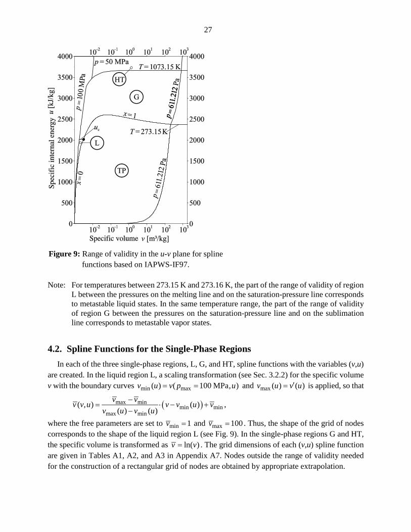
This range of validity corresponds to that of IAPWS-IF97, except for the lower pressure limit, which is set to s (273.15 K) 611.212 Pa.=p Figure 9 shows the range of validity and the defined regions of the spline functions with the variables (v,u). The single phase is divided into the liquid region L, the gas region G, and the high-temperature region HT. With regard to regions defined in IAPWS-IF97, the current liquid region L covers region 1 and a part of region 3. Region 2 and the remaining part of region 3 are included in the gas region G. The spline functions are smoothed at the IF97 region boundaries 1-3 and 2-3. The two-phase region TP corresponds to region 4 of IAPWS-IF97 and the high temperature region HT matches region 5 of IAPWS-IF97.

The specific internal energy at the critical point uc = 2019.025 106 kJ/kg is used to define the boundary between the L and G single-phase regions for supercritical state points. At the region boundaries L/G and G/HT in the single-phase region, small inconsistencies are unavoidable (see Sec. 4.6). These should be negligible for most purposes, but if needed the transition at these boundaries can be smoothed with simple interpolation equations.

Figure 8: Property calculations from (v,u), (p,v), and (u,s).

27

Note: For temperatures between 273.15 K and 273.16 K, the part of the range of validity of region L between the pressures on the melting line and on the saturation-pressure line corresponds to metastable liquid states. In the same temperature range, the part of the range of validity of region G between the pressures on the saturation-pressure line and on the sublimation line corresponds to metastable vapor states.

4.2. Spline Functions for the Single-Phase Regions In each of the three single-phase regions, L, G, and HT, spline functions with the variables (v,u)

are created. In the liquid region L, a scaling transformation (see Sec. 3.2.2) for the specific volume v with the boundary curves min max( ) ( 100 MPa, )= =v u v p u and max ( ) ( )′=v u v u is applied, so that

( )max minmin min

max min( , ) ( )

( ) ( )−

= ⋅ − +−

v vv v u v v u vv u v u

,

where the free parameters are set to min 1=v and max 100=v . Thus, the shape of the grid of nodes corresponds to the shape of the liquid region L (see Fig. 9). In the single-phase regions G and HT, the specific volume is transformed as ln( )=v v . The grid dimensions of each (v,u) spline function are given in Tables A1, A2, and A3 in Appendix A7. Nodes outside the range of validity needed for the construction of a rectangular grid of nodes are obtained by appropriate extrapolation.

Figure 9: Range of validity in the u-v plane for spline functions based on IAPWS-IF97.

28

From the single-phase spline functions SPL ( , )p v u and SPL ( , )s v u , the inverse spline functions INV ( , )u p v and INV ( , )v u s are determined as described in Sec. 3.2.3. With these inverse spline

functions, all remaining properties are calculated from (p,v) and (u,s), as illustrated in Fig. 8.

4.3. Calculations in the Two-Phase Region The properties in the two-phase region TP are calculated with the spline functions in the single-

phase regions L and G, along with additional constraints for the phase equilibrium. For process simulations where the range of states does not include the liquid region L or where small inconsistencies at the saturated liquid line are tolerable, the calculation can be simplified with spline functions for ( )′′v p , ( )′v u , and ( )′u T as discussed in Sec. 3.2.5. This simplification is applied to the spline functions of (v,u) and their inverse functions of (p,v) and (u,s) for the two-phase region TP described in this document. The algorithms are described in Appendices A4, A5, and A6. Auxiliary spline functions AUX

s ( , )p v u and AUXs ( , )p u s were created to provide initial

guesses for the calculations from (v,u) and (u,s). A comprehensive description of all algorithms for calculating the properties in the two-phase region is given in [11].

4.4. Derivatives The following derivatives are frequently required in CFD:

∂ ∂ u

pv

, ∂ ∂ v

pu

, ∂ ∂ p

uv

,

∂ ∂ u

Tv

, ∂ ∂ v

Tu

, and ∂ ∂ T

uv

.

These derivatives are calculated analytically from SPL ( , )p v u and SPL ( , )T v u . The derivatives are continuous and can therefore be applied in numerical calculations, e.g., to prepare a Jacobian matrix in CFD. However, any thermodynamic property where high accuracy is required should be obtained from a dedicated spline function, rather than using derivatives of other spline functions. A description of the calculation of derivatives is given in Sec. 3.2.4 and more detailed information is given in [11].

4.5. Deviations from IAPWS-IF97 The maximum (max) and root-mean-square (RMS) deviations between the spline functions

implemented as discussed in Secs. 4.2 and 4.3 and IAPWS-IF97, along with the permissible values (perm), are given in Tables 1 through 5. The permissible values were set by the IAPWS Task Group “CFD Steam Property Formulation” to ensure that the differences in the results of process simulations with the SBTL method from those obtained with the direct application of IAPWS-IF97 are negligible. The permissible values are less than or equal to the required numerical consistencies for the IAPWS-IF97 backward equations [2, 6, 7, 8, 9].

29

Table 1: Deviations in pressure p(v,u) from IAPWS-IF97

IF97 Region perm∆p

max∆p ( )RMS∆p

1 2.5MPa≤p 0.6 % 0.12 % 0.012 %

2.5MPa>p 15 kPa 0.61 kPa 0.0044 kPa

2 0.001 % 0.000 48 % 0.000 12 % 3 0.001 % 0.000 95 % 0.000 04 % 4 0.0035 % 0.0035 % 0.000 28 % 5 0.001 % 0.000 53 % 0.000 15 %

Table 2: Deviations in temperature T(v,u) from IAPWS-IF97

IF97 Region [ ]perm mK∆T [ ]max mK∆T ( ) [ ]RMS mK∆T

1 1 0.27 0.015 2 1 0.43 0.018 3 1 0.53 0.032

4 1 0.69 a 0.30 a

5 1 0.38 0.018 a Except for near-critical temperatures [(Tc−T) < 1.5 K].

Table 3: Deviations in specific entropy s(v,u) from IAPWS-IF97

IF97 Region ( )

m

6

per

10 kJ/ kg K−

∆

s

( )x

6ma

10 kJ/ kg K−

∆

s

( )

( )S

6RM

10 kJ/ kg K−

∆

s

1 1 0.74 0.049 2 1 0.34 0.045 3 1 0.52 0.022 4 1 0.34 0.044 5 1 0.87 0.056

30

Table 4: Deviations in speed of sound w(v,u) from IAPWS-IF97

IF97 Region perm∆w

max∆w ( )RMS∆w

1 0.001 % 0.000 92 % 0.000 007 % 2 0.001 % 0.000 77 % 0.000 008 %

3 0.001 % 0.000 56 % a 0.000 031 % a

5 0.001 % 0.000 42 % 0.000 005 % a In the vicinity of the critical point, the deviations of w are larger (< 0.02 %).

Table 5: Deviations in dynamic viscosity η(v,u) from IAPWS-IF97 and the IAPWS viscosity release with recommendations for industrial use [14]

IF97 Region permη∆

maxη∆ ( )RMSη∆

1 0.001 % 0.000 41 % 0.000 068 % 2 0.001 % 0.000 15 % 0.000 010 % 3 0.001 % 0.000 32 % 0.000 019 %

4.6. Numerical Consistency at Region Boundaries The specific internal energy at the critical point uc = 2019.025 106 kJ/kg defines the region

boundary between the liquid region L and the gas region G for supercritical state points (see Fig. 9). This boundary is within IAPWS-IF97 region 3. The numerical inconsistencies of the adjacent spline functions at the region boundary L-G result from the deviations between the spline functions and the basic equation of IAPWS-IF97 region 3 (see Sec. 4.5), and are given in Table 6.

Table 6: Numerical inconsistencies at the region boundaries L-G and G-HT

Region boundary max∆p max∆T max∆s max∆w maxη∆

L-G a 0.0011 % 0.38 mK 4.8×10-4 J kg-1 K-1 0.000 46 % 0.000 27 % G-HT b 0.023 % 82 mK 0.082 J kg-1 K-1 0.050 % - c

a These values were obtained from the corresponding (v,u)-spline functions for regions L and G at constant specific internal energy uc = 2019.025 106 kJ/kg.

b These values were obtained from the corresponding (v,u)-spline functions for regions G and HT at T = 1073.15 K.

c Since the upper temperature limit of the IAPWS viscosity release [14] is 1173.15 K, a spline function for the dynamic viscosity η in the high-temperature region is not provided.

31

The region boundary between the gas region G and the high-temperature region HT is identical to the IAPWS-IF97 region boundary 2-5 and follows the isotherm T = 1073.15 K. The underlying IAPWS-IF97 property functions have small discontinuities at the region boundary 2-5. The spline functions reproduce the results of the IAPWS-IF97 basic equations 2 and 5 with high accuracy. Thus, at the region boundary G-HT, the numerical inconsistencies of the IAPWS-IF97 basic equations (see [2]) are dominant; these are given in Table 6.

4.7. Computing-Time Comparisons The computing times of the spline functions have been evaluated and compared with those of

calculations with iterations of the IAPWS-IF97 basic equations. The Computing-Time Ratio (CTR) is defined as follows:

Computing time for the iterative calculation from IAPWS-IF97Computing time for the calculation from the SBTL function

=CTR .

IAPWS-IF97 property functions were computed from the Extended IAPWS-IF97 Steam Tables software [15]. Since the region definitions of the SBTL functions are different from the regions of IAPWS-IF97, the computing times of both formulations include the determination of the region that corresponds to the given state point. Neither IAPWS-IF97 nor the SBTL implementation takes advantage of information from previously calculated state points. The computing times were measured by means of software similar to NIFBENCH [2] with 100,000 randomly distributed state points in the corresponding region. All algorithms have been compiled into single-threaded software with the Intel Composer 2011 with default options. The tests were carried out on a Windows 8 computer equipped with an Intel Core i7-4500U CPU with 2.39 GHz and 8 GB RAM. The results of the computing-time comparisons are summarized in Table 7.

32

Table 7: Computing-time ratios (CTR) of spline-based property functions in comparison to the iterative calculations from IAPWS-IF97

IAPWS-IF97 Region SBTL function 1 2 3 4 5

p(v,u) 130 271 161 19.6 470 T(v,u) 161 250 158 20.6 442 s(v,u) 164 261 160 17.8 449 w(v,u) 199 310 234 - a 471

η(v,u) 197 309 239 - a - b

u(p,v) 2.0 6.4 2.8 5.6 3.2 v(u,s) 43.5 66.4 78.8 16.2 134

a Speed of sound w and dynamic viscosity η are not defined in the two-phase region. b Since the upper temperature limit of the IAPWS viscosity release [14] is 1173.15 K, a spline

function for the dynamic viscosity η in the high-temperature region is not provided.

33

5. Spline Functions of (p,h) and Inverse Functions Based on IAPWS-IF97 In heat cycle calculations, water and steam properties are frequently calculated from (p,h).

Therefore, another set of spline functions has been created for the calculation of , , , , ( , )η =T v s w f p h in the single-phase region. Furthermore, numerically consistent property

functions of (p,T), (p,s), and (h,s) are required. These are calculated through the use of inverse spline functions as described in Sec. 3.2.3. The relations between the spline and inverse spline functions are illustrated in Fig. 10. The properties in the two-phase region are calculated as explained in Sec. 5.3.

5.1. Range of Validity The range of validity is bounded as follows:

273.15 K 1073.15 K≤ ≤T 611.212 Pa 100 MPa≤ ≤p , 1073.15 K 2273.15 K< ≤T 611.212 Pa 50 MPa≤ ≤p .

This range of validity corresponds to IAPWS-IF97, except the lower pressure limit, which is set to s (273.15 K) 611.212 Pa.=p Figure 11 shows the range of validity and the defined regions of the

spline functions with the variables (p,h). The single phase is divided into the liquid region L, the gas region G, and the high temperature region HT. With regard to IAPWS-IF97, the liquid region L covers region 1 and a part of region 3. Region 2 and the remaining part of region 3 are included in the gas region G. The spline functions are smoothed at the IF97 region boundaries 1-3 and 2-3. The two-phase region TP corresponds to region 4 of IAPWS-IF97, and the high-temperature region HT matches region 5 of IAPWS-IF97.

The specific enthalpy at the critical point hc = 2087.546 845 kJ/kg is used to describe the boundary between the L and G single-phase regions for supercritical state points. At the region boundaries in the single-phase region, small inconsistencies are unavoidable (see Sec. 5.6). These should be negligible for most purposes, but if needed, the transition at these boundaries can be smoothed with simple interpolation equations.

Figure 10: Property calculations from (p,h), (p,T), (p,s), and (h,s).

34

Note: For temperatures between 273.15 K and 273.16 K, see the note at the end of Sec. 4.1.

5.2. Spline Functions for the Single-Phase Regions In each of the three single-phase regions, L, G, and HT, spline functions with the variables (p,h)

are created. These spline functions are constructed on rectangular grids without scaling transformations. Variable transformations have been applied to v(p,h), s(p,h), and w(p,h). The variable transformations and grid dimensions of each (p,h) spline function are given in Tables A4, A5, and A6 in Appendix A7. Nodes outside the range of validity needed for the construction of a rectangular grid of nodes are obtained by appropriate extrapolation.

From the spline functions SPL ( , )T p h and SPL ( , )s p h for the single phase, the inverse spline functions INV ( , )h p T , INV ( , )h p s , and INV ( , )p h s are determined as described in Sec. 3.2.3. All remaining properties can be calculated from these inverse spline functions with the input variables (p,T), (p,s), and (h,s) as illustrated in Fig. 11.

5.3. Calculations in the Two-Phase Region The properties in the two-phase region TP are calculated with the spline functions in the single-

phase regions L and G, along with additional constraints for phase equilibrium. For property

Figure 11: Range of validity in the p-h plane for spline functions based on IAPWS-IF97.

35

calculations from (p,h) and (p,s) in the two-phase region, the saturation temperature sT is calculated from a spline function s ( )T p based on the corresponding equation of IAPWS-IF97. The enthalpies of the saturated liquid and the saturated vapor are determined from the inverse spline functions

L ( , )h p T and G ( , )h p T . The corresponding algorithms are described in Appendices A1 and A2. For a given enthalpy and entropy (h,s), fluid properties in the two-phase region must be determined by iteration as shown in Appendix A3. For this purpose, an auxiliary spline function AUX

s ( , )p h s was created to provide an initial guess. A comprehensive description of all algorithms to calculate the properties in the two-phase region is given in [11].

5.4. Derivatives In heat cycle simulations, derivatives such as:

∂ ∂ h

Tp

, ∂ ∂ p

hT

, and ∂ ∂ T

hp

are frequently used. These derivatives are calculated analytically from SPL ( , )T p h . The derivatives are continuous and can therefore be applied in numerical calculations, e.g., to prepare a Jacobian matrix in heat cycle simulation software. However, any thermodynamic property where high accuracy is required should be obtained from a dedicated spline function. A description of the calculation of derivatives is given Sec. 3.2.4, and more detailed information is given in [11].

5.5. Deviations from IAPWS-IF97 The maximum (max) and root-mean-square (RMS) deviations between the spline functions and

IAPWS-IF97, along with the permissible values (perm), are given in Tables 8 through 12. The permissible values were set by the IAPWS Task Group “CFD Steam Property Formulation” to ensure that the differences in the results of process simulations with the SBTL method from those obtained with the direct application of IAPWS-IF97 are negligible. The permissible values are less than or equal to the required numerical consistencies for the IAPWS-IF97 backward equations [2, 6, 7, 8, 9].

Table 8: Deviations in temperature T(p,h) from IAPWS-IF97

IF97 Region [ ]perm mK∆T [ ]max mK∆T ( ) [ ]RMS mK∆T

1 25 0.63 0.073 2 10 0.81 0.026 3 25 0.65 0.045 5 10 0.34 0.042

36

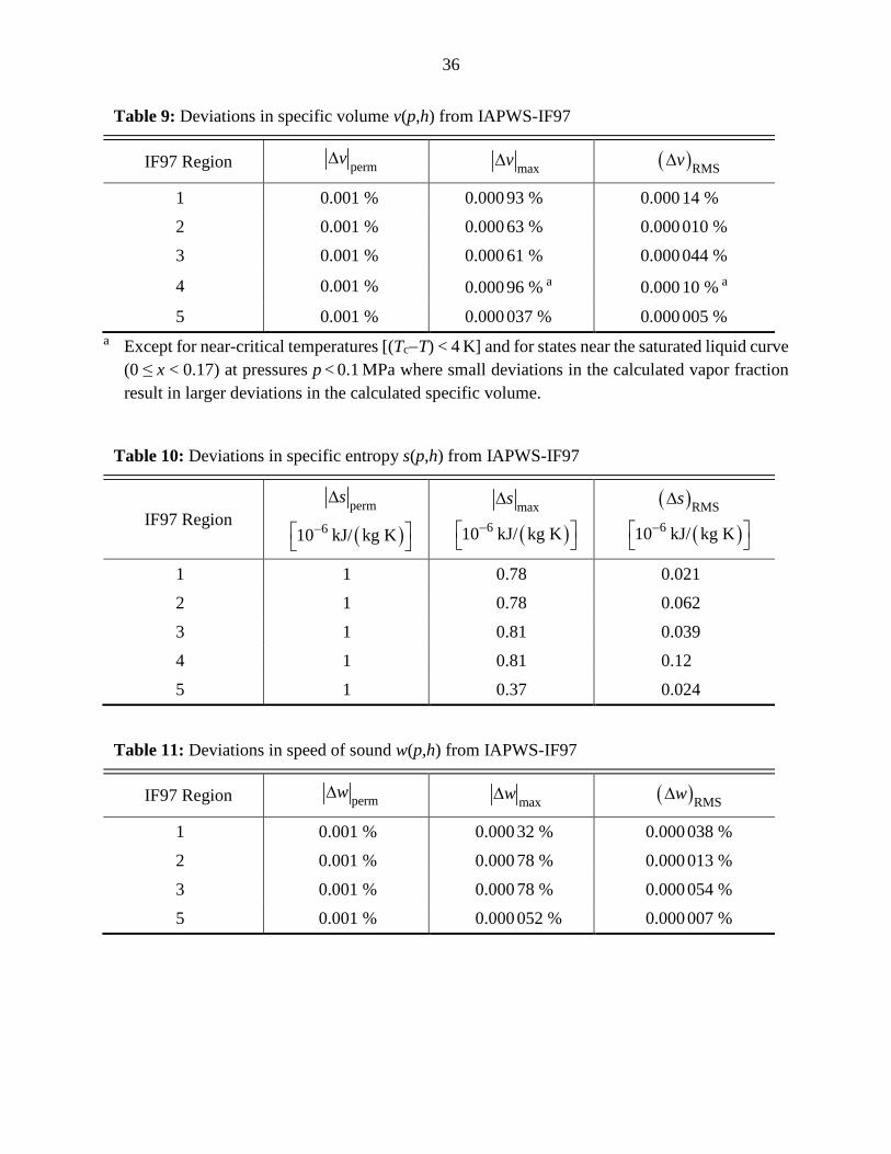
Table 9: Deviations in specific volume v(p,h) from IAPWS-IF97

IF97 Region perm∆v

max∆v ( )RMS∆v

1 0.001 % 0.000 93 % 0.000 14 % 2 0.001 % 0.000 63 % 0.000 010 % 3 0.001 % 0.000 61 % 0.000 044 %

4 0.001 % 0.000 96 % a 0.000 10 % a

5 0.001 % 0.000 037 % 0.000 005 % a Except for near-critical temperatures [(Tc−T) < 4 K] and for states near the saturated liquid curve

(0 ≤ x < 0.17) at pressures p < 0.1 MPa where small deviations in the calculated vapor fraction result in larger deviations in the calculated specific volume.

Table 10: Deviations in specific entropy s(p,h) from IAPWS-IF97

IF97 Region ( )

m

6

per

10 kJ/ kg K−

∆

s

( )x

6ma

10 kJ/ kg K−

∆

s

( )

( )S

6RM

10 kJ/ kg K−

∆

s

1 1 0.78 0.021 2 1 0.78 0.062 3 1 0.81 0.039 4 1 0.81 0.12 5 1 0.37 0.024

Table 11: Deviations in speed of sound w(p,h) from IAPWS-IF97

IF97 Region perm∆w

max∆w ( )RMS∆w

1 0.001 % 0.000 32 % 0.000 038 % 2 0.001 % 0.000 78 % 0.000 013 % 3 0.001 % 0.000 78 % 0.000 054 % 5 0.001 % 0.000 052 % 0.000 007 %

37

Table 12: Deviations in dynamic viscosity η(p,h) from IAPWS-IF97 and the IAPWS viscosity release with recommendations for industrial use [14]

IF97 Region permη∆

maxη∆ ( )RMSη∆

1 0.001 % 0.000 63 % 0.000 077 % 2 0.001 % 0.000 77 % 0.000 014 % 3 0.001 % 0.000 80 % 0.000 033 %

5.6. Numerical Consistency at Region Boundaries The specific enthalpy at the critical point hc = 2087.546 845 kJ/kg defines the boundary between

the liquid region L and the gas region G above the critical pressure (see Fig. 11). This boundary is within IAPWS-IF97 region 3. The numerical inconsistencies of the adjacent spline functions at the region boundary L-G result from the deviations between the spline functions and the basic equation of IAPWS-IF97 region 3 (see Sec. 5.5) and are given in Table 13.

The region boundary between the gas region G and the high-temperature region HT is identical to the IAPWS-IF97 region boundary 2-5 and follows the isotherm T = 1073.15 K. The underlying IAPWS-IF97 property functions have small discontinuities at the region boundary 2-5. The spline functions reproduce the results of the IAPWS-IF97 basic equations 2 and 5 with high accuracy. Thus, at the region boundary G-HT, the numerical inconsistencies of the IAPWS-IF97 basic equations (see [2]) are dominant; these are given in Table 13 and are in agreement with those from the IAPWS-IF97 basic equations at the region boundary 2-5.

Table 13: Numerical inconsistencies at the region boundaries L-G and G-HT

Region boundary max∆T or max∆h max∆v max∆s max∆w maxη∆

L-G a max∆T = 0.30 mK 0.000 70 % 3.9×10-5 J kg-1 K-1 0.000 51 % 0.000 33 %

G-HT b max∆h = 0.096 kJ kg-1 0.012 % 0.142 J kg-1 K-1 0.046 % - c a These values were obtained from the corresponding (p,h)-spline functions for regions L and G

at hc = 2087.546 845 kJ/kg. b These values were obtained from the inverse spline functions G ( , )h p T and HT ( , )h p T and the

corresponding (p,h)-spline functions at T = 1073.15 K. c Since the upper temperature limit of the IAPWS viscosity release [14] is 1173.15 K, a spline

function for the dynamic viscosity η in the high-temperature region is not provided.

38

5.7. Computing-Time Comparisons The computing times of the spline functions have been evaluated and compared with those of

IAPWS-IF97, where these functions are calculated from the basic equations, or, where available, from backward equations. The Computing-Time Ratio (CTR) is defined as follows:

Computing time of the calculation from IAPWS-IF97 basic eq. or backward eq.Computing time of the calculation from the SBTL algorithms

=CTR .

The IAPWS-IF97 property functions were computed from the Extended IAPWS-IF97 Steam Tables software [15]. Since the subdivision of the range of validity of the SBTL functions is different from the regions of IAPWS-IF97, the computing times of both formulations include the determination of the region that corresponds to the given state point. Neither IAPWS-IF97 nor the SBTL implementation takes advantage of information from previously calculated state points. The computing times were measured by means of software similar to NIFBENCH [2] with 100,000 randomly distributed state points in the corresponding region. The compiler and computer used were described in Sec. 4.7. The results of the computing-time comparisons are summarized in Table 14.

For the IAPWS-IF97 timing determinations, backward and boundary equations were used for calculations from (p,h), (p,s), and (h,s), and from (p,T) in region 3, where available (see [2, 6, 7, 8, 9]). The numerical consistency between the backward equations and the basic equations of IAPWS-IF97 might be insufficient for extensive heat cycle simulations and in particular for non-stationary processes. In such situations, backward functions are calculated by iteration from the IAPWS-IF97 basic equations with starting values obtained from the backward equations. The CTR values of the iteratively calculated backward functions are higher than the values in Table 14.

The test results given in [16, 17] show that the SBTL functions from (p,h), (p,s), and (h,s) are between 10 and 20 times faster than the iterative calculation from the IAPWS-IF97 basic equations with starting values from backward equations. More details on computing-time comparisons between calculations from backward equations and iterative calculations from the IAPWS-IF97 basic equations are summarized in [18]. With the SBTL method, the specific enthalpy h(p,T) is computed from the inverse spline function of T(p,h), thus being numerically consistent with this function. This procedure is slower than the calculation of h(p,T) in IAPWS-IF97 regions 1, 2, and 5 with the direct use of the basic equations. In heat cycle simulations, functions are generally less frequently calculated from (p,T). Analogously, the SBTL function h(p,s) is computed from the inverse spline function of s(p,h), and T(p,s) is calculated from T(p,h(p,s)). Therefore, these functions are numerically consistent with each other.

39

Table 14: Computing-time ratios (CTR) of spline-based property functions in comparison to the calculation from IAPWS-IF97 basic equations or backward equations

IAPWS-IF97 Region SBTL function 1 2 3 4 5

T(p,h) 2.9 4.7 3.0 4.4 26.5 v(p,h) 3.8 6.1 5.1 2.6 25.2 s(p,h) 3.8 5.7 5.7 2.9 12.8 w(p,h) 5.0 10.1 8.2 -a 30.0

η(p,h) 5.6 9.2 7.9 -a -b

h(p,T) 0.94 0.71 1.5 -c 0.34 h(p,s) 0.74 1.2 1.4 1.9 4.6 T(p,s) 0.50 0.94 0.76 1.0 3.8 p(h,s) 2.2 11.7 1.8 5.6 64.3 T(h,s) 2.0 8.6 1.7 5.8 52.6

a Speed of sound w and dynamic viscosity η are not defined in the two-phase region. b Since the upper temperature limit of the IAPWS viscosity release [14] is 1173.15 K, a spline

function for the dynamic viscosity η in the high-temperature region is not provided. c State points in the two-phase region are not uniquely defined with (p,T) inputs.

40

6. Spline Functions for the Metastable-Vapor Region Based on IAPWS-IF97 The industrial formulation IAPWS-IF97 [2, 3] provides a supplementary equation for part of

the metastable-vapor region. This equation is valid from the saturated vapor curve to the 5% equilibrium moisture line (determined from the equilibrium ′h and ′′h values) at pressures from the triple-point pressure up to 10 MPa.

Spline-based property functions of (v,u) and (p,h) have been developed for calculations in the metastable-vapor region described above. In order to avoid discontinuities at the saturated vapor curve, the range of validity of these spline functions has been extended to the gas region G as shown in Figs. 9 and 11. The spline functions are described in Sections 6.1 and 6.2, and are recommended for use in non-equilibrium process simulations. For simulating equilibrium processes, the spline functions described in Secs. 4 and 5 should be used.

6.1. Spline Functions of (v,u) Spline-based property functions for calculating , , , , ( , )η =p T s w f v u in both the metastable-

vapor region and the gas region G (see Fig. 9) have been created. For every spline-based property function of (v,u), the specific volume is transformed as ln( )=v v . The grid dimensions of these functions are equal to those given for the gas region G in Sec. 4.2 (see Table A2 in Appendix A7). Nodes outside the range of validity needed for the construction of a rectangular grid of nodes are obtained by appropriate extrapolation.

6.1.1. Deviations from IAPWS-IF97 The deviations of the developed spline-based property functions from the IAPWS-IF97

supplementary equation for the metastable-vapor region and from the IAPWS-IF97 basic equation for region 2, along with the permissible (perm) values, are given in Table 15. At the saturated vapor curve for pressures p < 10 MPa, increased deviations due to the small inconsistency between the IAPWS-IF97 supplementary equation for the metastable-vapor region and the IAPWS-IF97 basic equation for region 2 cannot be avoided. The maximum deviations (max) in the metastable-vapor region and in region 2 of IAPWS-IF97 outside the temperature ranges ( )s−T T p and the maximum deviations (max, sat) within these ranges are given in Table 15. The root-mean-square deviations (RMS) of the spline-based property functions from the IAPWS-IF97 supplementary equation for the metastable-vapor region and from the IAPWS-IF97 basic equation for region 2 are also given in Table 15.

41

Table 15: Deviations in pressure p(v,u), temperature T(v,u), specific entropy s(v,u), speed of sound w(v,u), and dynamic viscosity η(v,u) from the supplementary equation for the metastable-vapor region and the basic equation for region 2 of IAPWS-IF97 and the IAPWS viscosity release with recommendations for industrial use [14]

Spline function

Permissible deviation

Maximum deviation in the metastable-vapor region

and in region 2 of IAPWS-IF97 outside the range ( )s−T T pdefined in the next column

Range ( )s−T T p along the saturated vapor curve for p < 10 MPa RMS deviation

in the metastable-vapor region and in region 2 of

IAPWS-IF97 ( )s−T T p Maximum deviation

p(v,u) perm 0.001%∆ =p max 0.000 97 %∆ =p 7 K max, sat 0.016 %∆ =p ( )RMS 0.000 34 %∆ =p

T(v,u) perm 1 mK∆ =T max 0.60 mK∆ =T 10 K max, sat 25.2 mK∆ =T ( )RMS 1 mK.1∆ =T

s(v,u) ( )

m6

per

1 10 kJ/ kg K−

∆

×

=s

( )x

6ma

0.45 10 kJ/ kg K−×

∆ =s 12 K

( )max,

4 sat

0.81 10 kJ/ kg K−

=

×

∆s

( )( )

S6RM

0.83 10 kJ/ kg K−×

∆ =s

w(v,u) perm 0.001%∆ =w max 0.000 88 %∆ =w 10 K max, sat 0.05 %∆ =w ( )RMS 0.0017 %∆ =w

η(v,u) perm 0.001%η∆ = max 0.000 96 %η∆ = 6 K max, sat 0.0082 %η∆ = ( )RMS 0.000 31%η∆ =

42

6.1.2. Computing-Time Comparisons In the metastable-vapor region for pressures up to 10 MPa, the computing times of the spline

functions have been evaluated and compared with those of IAPWS-IF97, where these functions are calculated by iteration from the corresponding supplementary equation. The Computing-Time Ratio (CTR) is defined as follows:

Computing time for the iterative calculation from IAPWS-IF97Computing time for the calculation from the SBTL function

=CTR .

IAPWS-IF97 property functions were computed from the Extended IAPWS-IF97 Steam Tables software [15]. Since the region definitions of the SBTL functions are different from the regions of IAPWS-IF97, the computing times of both formulations include the determination of the region that corresponds to the given state point. Neither IAPWS-IF97 nor the SBTL implementation takes advantage of information from previously calculated state points. The computing times were measured by means of software similar to NIFBENCH [2] with 100,000 randomly distributed state points in the corresponding region. The compiler and computer used were described in Sec. 4.7. The results of the computing-time comparisons are summarized in Table 16.

Table 16: Computing-time ratios (CTR) of spline-based property functions compared to the iterative calculations from the IAPWS-IF97 supplementary equation for the metastable-vapor region

SBTL function

p(v,u) T(v,u) s(v,u) w(v,u) η(v,u)

CTR 88.3 86.4 89.5 87.0 90.0

6.2. Spline Functions of (p,h) Spline-based property functions for calculating , , , , ( , )η =T v s w f p h in both the metastable-vapor region and the gas region G (see Fig. 11) have been created. Variable transformations have been applied to v(p,h), s(p,h), and w(p,h). The variable transformations and grid dimensions of each (p,h) spline function are given in Table A7 in Appendix A7. Nodes outside the range of validity needed for the construction of a rectangular grid of nodes are obtained by appropriate extrapolation.

43

Table 17: Deviations in temperature T(p,h), specific volume v(p,h), specific entropy s(p,h), speed of sound w(p,h), and dynamic viscosity η(p,h) from the supplementary equation for the metastable-vapor region and the basic equation for region 2 of IAPWS-IF97 and the IAPWS viscosity release with recommendations for industrial use [14]

Spline function

Permissible deviation

Maximum deviation in the metastable-vapor region

and in region 2 of IAPWS-IF97 outside the range ( )s−T T pdefined in the next column

Range ( )s−T T p along the saturated vapor curve for p < 10 MPa RMS deviation

in the metastable-vapor region and in region 2 of

IAPWS-IF97 ( )s−T T p Maximum deviation

T(p,h) perm 1 mK∆ =T max 0.90 mK∆ =T 8 K max, sat 18.4 mK∆ =T

( )RMS 0.6 mK8∆ =T

v(p,h) perm 0.001%∆ =v max 0.000 60 %∆ =v 10 K max, sat 0.018 %∆ =v

( )RMS 0.000 28 %∆ =v

s(p,h) ( )m

6per

1 10 kJ/ kg K−

∆

×

=s

( )x

6ma

0.54 10 kJ/ kg K−×

∆ =s 16 K

( )max,

4 sat

0.84 10 kJ/ kg K−

=

×

∆s

( )

( )S

6RM

0.85 10 kJ/ kg K−×

∆ =s

w(p,h) perm 0.001%∆ =w max 0.000 89 %∆ =w

13 K max, sat 0.045 %∆ =w ( )RMS 0.0011 %∆ =w

η(p,h) perm 0.001%η∆ = max 0.000 80 %η∆ = 6 K max, sat 0.0061%η∆ =

( )RMS 0.00015 %η∆ =

44

6.2.1. Deviations from IAPWS-IF97 The deviations of the developed spline-based property functions from the IAPWS-IF97

supplementary equation for the metastable-vapor region and from the IAPWS-IF97 basic equation for region 2, along with the permissible (perm) values, are given in Table 17. At the saturated vapor curve for pressures p < 10 MPa, increased deviations due to the small inconsistency between the IAPWS-IF97 supplementary equation for the metastable-vapor region and the IAPWS-IF97 basic equation for region 2 cannot be avoided. The maximum deviations (max) in the metastable-vapor region and in region 2 of IAPWS-IF97 outside the temperature ranges ( )s−T T p and the maximum deviations (max, sat) within these ranges are given in Table 17. The root-mean-square deviations (RMS) of the spline-based property functions from the IAPWS-IF97 supplementary equation for the metastable-vapor region and from the IAPWS-IF97 basic equation for region 2 are also given in Table 17.

6.2.2. Computing-Time Comparisons In the metastable-vapor region for pressures up to 10 MPa, the computing times of the spline

functions have been evaluated and compared with those of IAPWS-IF97, where these functions are calculated by iteration from the corresponding supplementary equation. The Computing-Time Ratio (CTR) is defined as follows:

Computing time for the iterative calculation from IAPWS-IF97Computing time for the calculation from the SBTL function

=CTR .

IAPWS-IF97 property functions were computed from the Extended IAPWS-IF97 Steam Tables software [15]. Since the region definitions of the SBTL functions are different from the regions of IAPWS-IF97, the computing times of both formulations include the determination of the region that corresponds to the given state point. Neither IAPWS-IF97 nor the SBTL implementation takes advantage of information from previously calculated state points. The computing times were measured by means of software similar to NIFBENCH [2] with 100,000 randomly distributed state points in the corresponding region. The compiler and computer used were described in Sec. 4.7. The results of the computing-time comparisons are summarized in Table 18.

Table 18: Computing-time ratios (CTR) of spline-based property functions compared to the iterative calculations from the IAPWS-IF97 supplementary equation for the metastable-vapor region

SBTL function

T(p,h) v(p,h) s(p,h) w(p,h) η(p,h)

CTR 16.0 16.0 12.1 15.7 19.0

45

7. Spline Functions Based on IAPWS-95 The IAPWS-95 formulation for general and scientific use [4, 5] is the most accurate

representation of the thermodynamic properties of water and steam. The IAPWS-IF97 formulation for industrial use [2, 3] and the supplementary releases [6, 7, 8, 9] were developed based on IAPWS-95 to meet specific needs for higher computing speeds in many industrial applications, particularly for the steam power industry. The range of validity of IAPWS-IF97 is divided into five regions, resulting in small inconsistencies at the region boundaries. In situations where these inconsistencies cannot be tolerated, and/or for general and scientific use where the more accurate IAPWS-95 formulation is preferred, it may be useful to apply similar spline techniques to IAPWS-95. In order to demonstrate the applicability of the SBTL method to IAPWS-95, several spline-based property functions for calculations from (v,u) and (p,h) have been developed. For simplicity in developing this example, spline functions covering the region of temperatures from 273.15 K to 1273.15 K and pressures up to 1000 MPa are described. This excludes a small portion of the range of validity of IAPWS-95 at high pressures and low temperatures, but application of the SBTL method in that region would be a straightforward extension.

7.1. Spline Functions of (v,u) Spline functions based on IAPWS-95 for the calculation of , , , ( , )=p T s w f v u in the single-

phase region were created analogously to those based on IAPWS-IF97 (see Sec. 4). The results of the computing-time comparisons are summarized in Sec. 7.3.

7.1.1. Range of Validity The range of validity covers the fluid range of state bounded as follows: 273.15 K 1273.15 K≤ ≤T 611.212 Pa 1000 MPa≤ ≤p .

This range of validity corresponds to that of IAPWS-95, except for the lower temperature limit, which is 273.15 K, and the lower pressure limit, which is s (273.15 K) 611.212 Pa.=p Figure 12 shows the range of validity and the defined regions of the spline functions with the variables (v,u). The range of validity is divided into the liquid region L, the gas region G, and the two-phase region TP. This division is similar to the division for IAPWS-IF97 shown in Fig. 9, except that no separate high-temperature region HT is needed.

The specific internal energy at the critical point uc = 2015.734 524 kJ/kg is used to define the boundary between regions L and G for supercritical state points. At the region boundary in the single-phase region, small inconsistencies are unavoidable. These should be negligible for most purposes, but if needed the transition at this boundary can be smoothed using simple interpolation equations.

46

Note: For temperatures between 273.15 K and 273.16 K, see the note at the end of Sec. 4.1.

7.1.2. Spline Functions for the Single-Phase Regions In each of the single-phase regions L and G, spline functions with the variables (v,u) were

created. In the liquid region L, a scaling transformation (see Sec. 3.2.2) for the specific volume v with the boundary curves ( )min max( 1000 MPa, )= =v u v p u and ( )max ( )′=v u v u is applied, so that

( ) ( ) ( )( )max minmin min

max min( , ) −

= ⋅ − +−

v vv v u v v u vv u v u

,

where the free parameters are set to min 1=v and max 100=v . Thus, the shape of the grid of nodes corresponds to the shape of the liquid region L (see Fig. 12). In the gas region G, the specific volume is transformed as ln( )=v v . The grid dimensions of each (v,u) spline function are given in Tables A8 and A9 in Appendix A7. Nodes outside the range of validity needed for the construction of a rectangular grid of nodes are obtained by appropriate extrapolation.

7.1.3. Deviations from IAPWS-95 The maximum (max) and root-mean-square (RMS) deviations between the spline functions and

IAPWS-95, along with the permissible values (perm), are given in Tables 19 through 22. The permissible values were set by the IAPWS Task Group “CFD Steam Property Formulation” to ensure that the differences in the results of process simulations with the SBTL method from those

Figure 12: Range of validity in the u-v plane for spline functions based on IAPWS-95.

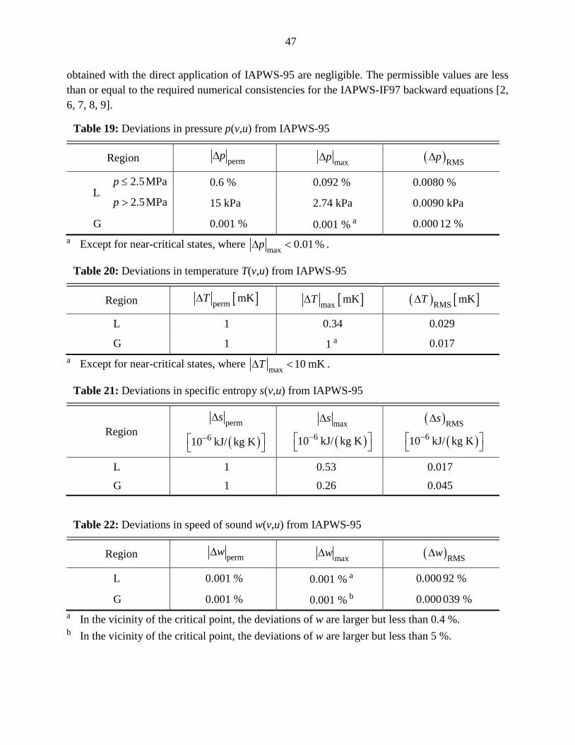
47

obtained with the direct application of IAPWS-95 are negligible. The permissible values are less than or equal to the required numerical consistencies for the IAPWS-IF97 backward equations [2, 6, 7, 8, 9].

Table 19: Deviations in pressure p(v,u) from IAPWS-95

Region perm∆p

max∆p ( )RMS∆p

L 2.5MPa≤p 0.6 % 0.092 % 0.0080 %

2.5MPa>p 15 kPa 2.74 kPa 0.0090 kPa

G 0.001 % 0.001 % a 0.000 12 % a Except for near-critical states, where max 0.01%∆ <p .

Table 20: Deviations in temperature T(v,u) from IAPWS-95

Region [ ]perm mK∆T [ ]max mK∆T ( ) [ ]RMS mK∆T

L 1 0.34 0.029

G 1 1 a 0.017 a Except for near-critical states, where max 10 mK∆ <T .

Table 21: Deviations in specific entropy s(v,u) from IAPWS-95

Region ( )

m

6

per

10 kJ/ kg K−

∆

s

( )x

6ma

10 kJ/ kg K−

∆

s

( )

( )S

6RM

10 kJ/ kg K−

∆

s

L 1 0.53 0.017 G 1 0.26 0.045

Table 22: Deviations in speed of sound w(v,u) from IAPWS-95

Region perm∆w

max∆w ( )RMS∆w

L 0.001 % 0.001 % a 0.000 92 %

G 0.001 % 0.001 % b 0.000 039 % a In the vicinity of the critical point, the deviations of w are larger but less than 0.4 %. b In the vicinity of the critical point, the deviations of w are larger but less than 5 %.

48

7.2. Spline Functions of (p,h) Spline functions based on IAPWS-95 for the calculation of , ( , )=T v f p h in the single-phase

region were created analogously to those based on IAPWS-IF97 (see Sec. 5). The results of the computing-time comparisons are summarized in Sec. 7.3.

7.2.1. Range of Validity The range of validity covers the fluid range of state bounded as follows: 273.15 K 1273.15 K≤ ≤T 611.212 Pa 1000 MPa≤ ≤p .

This range of validity corresponds to that of IAPWS-95, except for the lower temperature limit, which is 273.15 K, and the lower pressure limit, which is s (273.15 K) 611.212 Pa.=p Figure 13 shows the range of validity and the defined regions of the spline functions with the variables (p,h). The range of validity is divided into the liquid region L, the gas region G, and the two-phase region TP. This division is similar to the division for IAPWS-IF97 shown in Fig. 11, except that no separate high-temperature region HT is needed.

The specific enthalpy at the critical point hc = 2084.256 263 kJ/kg is used to define the boundary between regions L and G for supercritical state points. At the region boundary in the single-phase region, small inconsistencies are unavoidable. These should be negligible for most purposes, but if needed the transition at this boundary can be smoothed using simple interpolation equations.

Note: For temperatures between 273.15 K and 273.16 K, see the note at the end of Sec. 4.1.

Figure 13: Range of validity in the p-h plane for spline functions based on IAPWS-95.

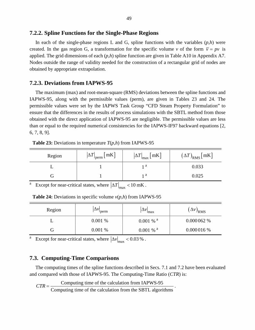
49

7.2.2. Spline Functions for the Single-Phase Regions In each of the single-phase regions L and G, spline functions with the variables (p,h) were

created. In the gas region G, a transformation for the specific volume v of the form =v pv is applied. The grid dimensions of each (p,h) spline function are given in Table A10 in Appendix A7. Nodes outside the range of validity needed for the construction of a rectangular grid of nodes are obtained by appropriate extrapolation.

7.2.3. Deviations from IAPWS-95 The maximum (max) and root-mean-square (RMS) deviations between the spline functions and

IAPWS-95, along with the permissible values (perm), are given in Tables 23 and 24. The permissible values were set by the IAPWS Task Group “CFD Steam Property Formulation” to ensure that the differences in the results of process simulations with the SBTL method from those obtained with the direct application of IAPWS-95 are negligible. The permissible values are less than or equal to the required numerical consistencies for the IAPWS-IF97 backward equations [2, 6, 7, 8, 9].

Table 23: Deviations in temperature T(p,h) from IAPWS-95

Region [ ]perm mK∆T [ ]max mK∆T ( ) [ ]RMS mK∆T

L 1 1 a 0.033

G 1 1 a 0.025 a Except for near-critical states, where max 10 mK∆ <T .

Table 24: Deviations in specific volume v(p,h) from IAPWS-95

Region perm∆v

max∆v ( )RMS∆v

L 0.001 % 0.001 % a 0.000 062 %

G 0.001 % 0.001 % a 0.000 016 % a Except for near-critical states, where max 0.03 %∆ <v .

7.3. Computing-Time Comparisons The computing times of the spline functions described in Secs. 7.1 and 7.2 have been evaluated

and compared with those of IAPWS-95. The Computing-Time Ratio (CTR) is:

Computing time of the calculation from IAPWS-95Computing time of the calculation from the SBTL algorithms

=CTR .

50

The IAPWS-95 property functions were computed from the internal routines of REFPROP [19] where the phase (liquid or vapor) is known and no phase tests are performed. Calculations from the IAPWS-95 fundamental equation and its derivatives are computationally intensive. In addition, depending on the considered property function, one- or two-dimensional iteration procedures are used in the REFPROP software. The resulting computing times are more than 100 times longer than for computations from SBTL functions. The computing times were measured by means of software similar to NIFBENCH [2] with 100,000 randomly distributed state points in the corresponding region. The compiler and computer used were described in Sec. 4.7. The results of the computing-time comparisons are summarized in Table 25.

Table 25: Computing-time ratios (CTR) of spline-based property functions compared to calculations from IAPWS-95

Region SBTL function L G

p(v,u) 243 434 T(v,u) 251 410

T(p,h) ≈15 000 6760

v(p,h) ≈14 500 6900

51

8. Application of the SBTL Method in Computational Fluid Dynamics In order to evaluate the usability of the SBTL method in extensive numerical process

simulations, the property functions described in Sec. 4 have been implemented into advanced CFD software and applied to several test cases [20, 21].

The numerical simulation of condensing steam flow around a fixed blade in a turbine stage, see [22], demonstrates the advantages of the SBTL method in CFD simulations for turbomachinery. Furthermore, turbulent steam flow through a duct has been simulated. Due to the numerical consistency of forward and backward spline functions, as well as consistency at the phase boundaries, the computation is very stable. In comparison to the direct IAPWS-IF97 implementation, the computing times of the CFD simulations were reduced by factors between 6 and 10 through the use of the SBTL functions. In comparison to CFD calculations where steam is considered to be an ideal gas, the computing time consumption with the SBTL functions is increased by a factor of only 1.4. The numerical results of the test cases described above show negligible differences from those obtained from simulations with the direct IAPWS-IF97 implementation, and are summarized in [20, 21].

9. Application of the SBTL Method in Heat Cycle Calculation Software In order to test the applicability of the SBTL method in heat cycle simulations, the property

functions described in Sec. 5 have been implemented in two different heat cycle simulation software tools [16, 17]. In comparison to the use of IAPWS-IF97, the overall computing time of a heat cycle calculation can be significantly reduced through the application of the SBTL method. The test calculations reported in [16] show that the computing times are reduced on average by a factor of 2. The engineering design parameters resulting from this different property calculation method differ negligibly (less than 0.02 %) from results obtained through the direct application of IAPWS-IF97.

10. Generating Spline Functions for User-Specified Demands The SBTL method has been developed for fast and accurate property calculations in extensive

process simulations. In order to apply this method to property functions for any fluid, the software FluidSplines [11, 23] has been developed. The fluid properties needed to generate the spline functions can be provided from external databases such as the property libraries from the Zittau/Goerlitz University of Applied Sciences or REFPROP [19] from NIST. FluidSplines implements all the features of the SBTL method (see Sec. 3 and [11]), and assists the user in generating spline functions and inverse spline functions for a given range of validity with a user-specified agreement with the underlying property formulations.

52

11. References [1] Kunick, M., Kretzschmar, H.-J., Gampe, U., di Mare, F., Hrubý, J., Duška, M., Vinš, V.,

Singh, A., Miyagawa, K., Weber, I., Pawellek, R., Novi, A., Blangetti, F., Friend, D.G., and Harvey, A.H., Fast Calculation of Steam and Water Properties with the Spline-Based Table Look-Up Method (SBTL), J. Eng. Gas Turbines & Power, in preparation.

[2] IAPWS, Revised Release on the IAPWS Industrial Formulation 1997 for the Thermodynamic Properties of Water and Steam (2007), available at http://www.iapws.org.

[3] Wagner, W., Cooper, J.R., Dittmann, A., Kijima, J., Kretzschmar, H.-J., Kruse, A., Mareš, R., Oguchi, K., Sato, H., Stöcker, I., Šifner, O., Takaishi, Y., Tanishita, I., Trübenbach, J., and Willkommen, Th., The IAPWS Industrial Formulation 1997 for the Thermodynamic Properties of Water and Steam, J. Eng. Gas Turbines & Power 122, 150-182 (2000).

[4] IAPWS, Revised Release on the IAPWS Formulation 1995 for the Thermodynamic Properties of Ordinary Water Substance for General and Scientific Use (2014), available at http://www.iapws.org.

[5] Wagner, W., and Pruß, A., The IAPWS Formulation 1995 for the Thermodynamic Properties of Ordinary Water Substance for General and Scientific Use, J. Phys. Chem. Ref. Data 31, 387-535 (2002).

[6] IAPWS, Revised Supplementary Release on Backward Equations for Pressure as a Function of Enthalpy and Entropy p(h,s) for Regions 1 and 2 of the IAPWS Industrial Formulation 1997 for the Thermodynamic Properties of Water and Steam (2014), available at http://www.iapws.org.

[7] IAPWS, Revised Supplementary Release on Backward Equations for the Functions T(p,h), v(p,h), and T(p,s), v(p,s) for Region 3 of the IAPWS Industrial Formulation 1997 for the Thermodynamic Properties of Water and Steam (2014), available at http://www.iapws.org.

[8] IAPWS, Revised Supplementary Release on Backward Equations p(h,s) for Region 3, Equations as a Function of h and s for the Region Boundaries, and an Equation Tsat(h,s) for Region 4 of the IAPWS Industrial Formulation 1997 for the Thermodynamic Properties of Water and Steam (2014), available at http://www.iapws.org.

[9] IAPWS, Revised Supplementary Release on Backward Equations for Specific Volume as a Function of Pressure and Temperature v(p,T) for Region 3 of the IAPWS Industrial Formulation 1997 for the Thermodynamic Properties of Water and Steam (2014), available at http://www.iapws.org.

[10] IAPWS, Guideline on the Tabular Taylor Series Expansion (TTSE) Method for Calculation of Thermodynamic Properties of Water and Steam Applied to IAPWS-95 as an Example (2003), available at http://www.iapws.org.

53

[11] Kunick, M., Fast Calculation of Thermophysical Properties in Extensive Process Simulations with the Spline-Based Table Look-Up Method (STBL), VDI Fortschritt-Berichte, in preparation.

[12] Späth, H., One Dimensional Spline Interpolation Algorithms, ISBN 1-56881-016-4, A K Peters (1995).

[13] Späth, H., Two Dimensional Spline Interpolation Algorithms, ISBN 1-56881-017-2, A K Peters (1995).

[14] IAPWS, Release on the IAPWS Formulation 2008 for the Viscosity of Ordinary Water Substance (2008), available at http://www.iapws.org.

[15] Wagner, W., and Overhoff, U., Extended IAPWS-IF97 Steam Tables, Springer-Verlag (2006).

[16] Bennoit, S., Test of the IAPWS SBTL Guideline in KRAWAL-modular, Report to IAPWS IRS Working Group (2014).

[17] Pawellek, R., Löw, T., and Maltsev, A., Evaluation of Spline Routines in EBSILON® Professional, Report to IAPWS IRS Working Group (2014).

[18] Wagner, W., and Kretzschmar, H.-J., International Steam Tables, Springer-Verlag (2008).

[19] Lemmon, E.W., Huber, M.L., and McLinden, M.O., NIST Standard Reference Database 23: Reference Fluid Thermodynamic and Transport Properties - REFPROP, National Institute of Standards and Technology, Standard Reference Data Program, Gaithersburg (2013).

[20] di Mare, F., Report on the Evaluation of the Spline-Based Table Look-Up Method (SBTL) in CPU-intensive 3D-CFD Applications, Report to IAPWS IRS Working Group (2014).

[21] Kunick, M., Kretzschmar, H.-J., di Mare, F., and Gampe, U., CFD Analysis of Steam Turbines with the IAPWS Standard on the Spline-Based Table Look-Up Method (SBTL) for the Fast Calculation of Real Fluid Properties, ASME Turbo Expo 2015: Turbine Technical Conference and Exposition, Vol. 8: Microturbines, Turbochargers and Small Turbomachines; Steam Turbines, ISBN: 978-0-7918-5679-6 (2015).

[22] White, A.J., Young, J.B., and Walters, P.T., Experimental Validation of Condensing Flow Theory for a Stationary Cascade of Steam Turbine Blades, Phil. Trans. R. Soc. Lond. A 354, 59-88 (1996).

[23] Kunick, M., and Kretzschmar, H.-J., FluidSplines – Software for Generating Spline Functions, information available at http://www.thermodynamics-zittau.de.

54

APPENDIX A1 Property Calculations in the Two-Phase Region from (p,h)

In order to calculate the properties in the two-phase region from (p,h), the following algorithm is recommended. In addition to the (p,h) spline functions in the liquid region L and gas region G, a function for s ( )T p and the inverse spline functions L ( , )h p T and G ( , )h p T are provided. From these functions, s s ( )=T T p , L

s( , )′ =h h p T , and Gs( , )′′ =h h p T are determined without iteration.

The vapor fraction x is calculated from ( ) / ( )′ ′′ ′= − −x h h h h and the desired mass-specific properties are calculated from ( )′ ′′ ′= + −z z x z z .

A2 Property Calculations in the Two-Phase Region from (p,s)

In order to calculate the properties in the two-phase region from (p,s), the following algorithm is recommended. In addition to the (p,h) spline functions in the liquid region L and gas region G, a function for s ( )T p and the inverse spline functions L ( , )h p T and G ( , )h p T are provided. From these functions s s ( )=T T p , L

s( , )′ =h h p T , Gs( , )′′ =h h p T , L ( , )′ ′=s s p h , and G ( , )′′ ′′=s s p h are

determined without iteration. The vapor fraction x is calculated from ( ) / ( )′ ′′ ′= − −x s s s s and the desired mass-specific properties are calculated from ( )′ ′′ ′= + −z z x z z .

A3 Property Calculations in the Two-Phase Region from (h,s)

In order to calculate the properties in the two-phase region from (h,s), the following algorithm is recommended. In addition to the (p,h) spline functions in the liquid region L and gas region G, a function for s ( )T p and the inverse spline functions L ( , )h p T and G ( , )h p T are provided.

With the use of a one-dimensional Newton iteration scheme, the equation

( ) ( ) ( )0= = −h sf p x p x p (A3.1)

is solved for the pressure p, where

( ) ( )( ) ( )

′−=

′′ ′−hh h p

x ph p h p

and ( ) ( )( ) ( )

′−=

′′ ′−ss s p

x ps p s p

. (A3.2, A3.3)

The iteration procedure is

( )( )

1 dd

+ = − kk k

k

f pp p f p

p

, (A3.4)

where

( ) ( ) ( )d ddd d d

= −h sk k k

x xf p p pp p p

. (A3.5)

In each iteration step k, s, s ( )=k kT T p is calculated with the corresponding spline function. From the inverse spline functions L ( , )h p T and G ( , )h p T , ( )′ kh p and ( )′′ kh p are determined as

55

Ls,( ) ( , )′ =k k kh p h p T and G

s,( ) ( , )′′ =k k kh p h p T . Then, L( ) ( , ( ))′ ′=k k ks p s p h p andG( ) ( , ( ))′′ ′′=k k ks p s p h p are subsequently calculated.

The derivatives in Eq. (A3.5) are calculated from

( )

d d dd d dd

d

′ ′′ ′ − − −

=′′ ′−

hh

h h hxp p px

p h h and

( )

d d dd d dd

d

′ ′′ ′ − − −

=′′ ′−

ss

s s sxp p px

p s s (A3.6, A3.7)

where

sddd d

′ ∂ ∂ = + ∂ ∂ pT

Th h hp p T p

, sddd d′′ ∂ ∂ = + ∂ ∂ pT

Th h hp p T p

, (A3.8, A3.9)

d dd d′ ′ ∂ ∂ = + ∂ ∂ ph

s s s hp p h p

, and d dd d′′ ′′ ∂ ∂ = + ∂ ∂ ph

s s s hp p h p

. (A3.10, A3.11)

In Eqs. (A3.8, A3.9, A3.10, A3.11), the derivatives

∂ ∂ T

hp

, ∂ ∂ p

hT

, ∂ ∂ h

sp

, and ∂ ∂ p

sh

are determined in the corresponding phase from L ( , )T p h , G ( , )T p h , L ( , )s p h , and G ( , )s p h . The saturation temperature gradient of the saturation curve is derived from s ( )T p . The iteration procedure is repeated until ≤f TOL and s = kp p , sT , x, ′h , ′′h , ′s , and ′′s are determined. A spline function for s ( , )p h s is used to initialize kp .

A4 Property Calculations in the Two-Phase Region from (v,u)

For property calculations where small inconsistencies at the saturated liquid line are tolerable, the following additional phase boundary conditions are recommended. In addition to the (v,u) spline functions in the liquid region L and the gas region G, spline functions for the properties at saturation ( )′′v p , ( )′v u , and ( )′u T are required. With the use of a one-dimensional Newton iteration scheme, the equation

( ) ( ) ( )0= = −v uf p x p x p (A4.1)

is solved for the pressure p, where

( ) ( )( ) ( )

′−=

′′ ′−vv v p

x pv p v p

and ( ) ( )( ) ( )

′−=

′′ ′−uu u p

x pu p u p

. (A4.2, A4.3)

The iteration procedure is

( )( )

1 dd

+ = − kk k

k

f pp p f p

p

, (A4.4)

56

where

( ) ( ) ( )d ddd d d

= −v uk k k

x xf p p pp p p

. (A4.5)

In each iteration step k, ( )′′ kv p is calculated with the corresponding spline function. From the inverse spline function G ( , )u p v , ( )′′ ku p is determined as G( ) ( , ( ))′′ ′′=k k ku p u p v p . Then,

Gs ( ) ( ( ), ( ))′′ ′′=k k kT p T v p u p , s( ) ( ( ))′ ′=k ku p u T p , and ( ) ( ( ))′ ′ ′=k kv p v u p are subsequently

calculated. The derivatives in Eq. (A4.5) are calculated from

( )

d d dd d dd

d

′ ′′ ′ − − −

=′′ ′−

vv

v v vxp p px

p v v and

( )

d d dd d dd

d

′ ′′ ′ − − −

=′′ ′−

uu

u u uxp p px

p u u, (A4.6, A4.7)

where

s

s

dd d dd d d d′ ′ ′=

′Tv v u

p u T p and s

s

dd dd d d

′ ′=

Tu up T p

. (A4.8, A4.9)

The derivatives

dd

′′

vu

and s

dd

′uT

in Eqs. (A4.8, A4.9) are derived from the spline functions ( )′v u and ( )′u T .

The saturation temperature gradient is calculated from

sd d dd d d

′′ ′′∂ ∂ = + ∂ ∂ u v

T T v T up v p u p

, (A4.10)

where

∂ ∂ u

Tv

and ∂ ∂ v

Tu

are determined in the gas phase from G ( , )T v u . The derivative

dd′′vp

is derived from ( )′′v p , and

d dd d′′ ′′ ∂ ∂ = + ∂ ∂ pv

u u u vp p v p

(A4.11)

is calculated with

∂ ∂ v

up

and ∂ ∂ p

uv

57

in the gas phase, which is derived from G ( , )p v u . The iteration procedure is repeated until ≤f TOL and s = kp p , sT , x, ′v , ′′v , ′u , and ′′u are determined. A spline function for s ( , )p v u is

used to initialize kp .

A5 Property Calculations in the Two-Phase Region from (p,v)

In order to calculate the properties in the two-phase region from (p,v) consistently with the calculations from (v,u) described in Appendix A4, the following algorithm is recommended. From the spline and inverse spline functions ( )′′v p , G ( , )u p v , G ( , )T v u , ( )′u T , and ( )′v u , the saturation properties are subsequently calculated from

( )′′ ′′=v v p , G ( , )′′ ′′=u u p v , Gs ( , )′′ ′′=T T v u , s( )′ ′=u u T , and ( )′ ′ ′=v v u

without iteration. The vapor fraction x is calculated from ( ) / ( )′ ′′ ′= − −x v v v v , and the desired mass-specific properties are calculated from ( )′ ′′ ′= + −z z x z z .

A6 Property Calculations in the Two-Phase Region from (u,s)

In order to calculate the properties in the two-phase region from (u,s) consistently with the calculations from (v,u) described in Appendix A4, the following algorithm is recommended. With the use of a one-dimensional Newton iteration scheme, the equation

( ) ( ) ( )0= = −u sf p x p x p (A6.1)

is solved for the pressure p, where

( ) ( )( ) ( )

′−=

′′ ′−uu u p

x pu p u p

and ( ) ( )( ) ( )

′−=

′′ ′−ss s p

x ps p s p

. (A6.2, A6.3)

The iteration procedure is

( )( )

1 dd

+ = − kk k

k

f pp p f p

p

, (A6.4)

where

( ) ( ) ( )d ddd d d

= −u sk k k

x xf p p pp p p

. (A6.5)

In each iteration step k, ( )′′ kv p is calculated with the corresponding spline function. From the inverse spline function G ( , )u p v , s,( )′′ ku p is determined as G

s, s, s,( ) ( , ( ))′′ ′′=k k ku p u p v p . Then, G

s, s, s,( ) ( ( ), ( ))′′ ′′ ′′=k k ks p s v p u p , Gs s, s, s,( ) ( ( ), ( ))′′ ′′=k k kT p T v p u p , s, s s,( ) ( ( ))′ ′=k ku p u T p ,

s, s,( ) ( ( ))′ ′ ′=k kv p v u p , and Ls, s, s,( ) ( ( ), ( ))′ ′ ′=k k ks p s v p u p are subsequently calculated. The

derivatives in Eq. (A6.5) are calculated from

58

( )

d d dd d dd

d

′ ′′ ′ − − −

=′′ ′−

uu

u u uxp p px

p u u and

( )

d d dd d dd

d

′ ′′ ′ − − −

=′′ ′−

ss

s s sxp p px

p s s (A6.6, A6.7)

where

s

s

dd dd d d

′ ′=

Tu up T p

and d d dd d d′ ′ ′∂ ∂ = + ∂ ∂ v u

s s u s vp u p v p

. (A6.8, A6.9)

In Eqn. (A6.8), the derivative

s

dd

′uT

is derived from the spline functions ( )′u T . The derivative

s

s

dd d dd d d d′ ′ ′=

′Tv v u

p u T p (A6.10)

is calculated with

dd

′′

vu

,

which is derived from ( )′v u . The saturation temperature gradient of the saturation curve is calculated from

sd d dd d d

′′ ′′∂ ∂ = + ∂ ∂ u v

T T v T up v p u p

, (A6.11)

where

∂ ∂ u

Tv

and ∂ ∂ v

Tu

are determined in the gas phase from G ( , )T v u . The derivative

dd′′vp

is derived from ( )′′v p , and

d dd d′′ ′′ ∂ ∂ = + ∂ ∂ pv

u u u vp p v p

(A6.12)

is calculated with

∂ ∂ v

up

and ∂ ∂ p

uv

59

in the gas phase derived from G ( , )p v u . The iteration procedure is repeated until ≤f TOL and s = kp p , sT , x, ′v , ′′v , ′u , ′′u , ′s , and ′′s are determined. A spline function for s ( , )p u s is used

to initialize kp .

A7 Transformations and Grid Dimensions

For each spline function described in Secs. 4, 5, 6, and 7, the transformations and dimensions of the grid of nodes are given in the tables below. For piecewise equidistant nodes, the domain of the considered transformed variable min max≤ ≤x x x is subdivided in several intervals with equidistant nodes. In the tables below, this is described with

min

max

nodes...

......

nodes

x

x,

where the boundaries of the intervals are given in the column on the left and the number of equidistant nodes between them is given in the column on the right.

60

Table A1: Transformations and dimensions of the grid of nodes of each (v,u) spline function for the liquid region L based on IAPWS-IF97 and the IAPWS viscosity release with recommendations for industrial use [13]

Spline function

v [m3/kg] u [kJ/kg]

( )max minmin min

max min( , ) ( )

( ) ( )−

= ⋅ − +−

v vv v u v v u vv u v u

min 1=v max 100=v

min

max

nodes...

......

nodes

v

v

min

max

nodes...

......

nodes

u

u

( )L ,p v u 1

10095

200100

8.489 68

250204

30

0. 1

02

025

−

( )L ,T v u [ ]1100

100

[ ]8.489 682040.

201

00

−

( )L ,s v u [ ]1100

100

8.489 68

2040.0

11

01

00

2 0

−

( )L ,w v u 1

10090

50100

8.489 68

2040.0

11

01

00

2 0

−

( )L ,η v u [ ]1100

100

8.489 68

2040.01

75300

150

−

61

Table A2: Transformations and dimensions of the grid of nodes of each (v,u) spline function for the gas region G based on IAPWS-IF97 and the IAPWS viscosity release with recommendations for industrial use [13]

Spline function

v [m3/kg] u [kJ/kg] ( ) ln( )=v v v

min

max

nodes...

......

nodes

v

v

min

max

nodes...

......

nodes

u

u

( )G ,p v u

( )G ,T v u

( )G ,s v u

( )G ,w v u

( )G ,η v u

( )( )( )

3

3

1.698 44 10150

8 10200

1004.42

−

−

×

×

v

v

v

2009.99

26503693.67

10075

Table A3: Transformations and dimensions of the grid of nodes of each (v,u) spline function for the high-temperature region HT based on IAPWS-IF97

Spline function

v [m3/kg] u [kJ/kg] ( ) ln( )=v v v

min

max

nodes...

......

nodes

v

v

min

max

nodes...

......

nodes

u

u

( )HT ,p v u

( )HT ,T v u

( )HT ,w v u

( )( )

[ ]37.456 81 10

2002212.94

− ×

v

v [ ]3432.75

756518.9

( )HT ,s v u ( )

( )[ ]

-37.344 62 10200

2112.08

×

v

v [ ]3408.16

1006364.93

62

Table A4: Transformations and dimensions of the grid of nodes of each (p,h) spline function for the liquid region L based on IAPWS-IF97 and the IAPWS viscosity release with recommendations for industrial use [13]

Spline function

p [MPa] h [kJ/kg]

( )p p

min

max

nodes...

......

nodes

p

p

min

max

nodes...

......

nodes

h

h

( )L ,T p h p

-4

-2

5 10100

1 10 7520 100

105

× ×

[ ]214

12.71 21 5

09

2

−

( )L ,v p h p

-4

-2

5 10100

1 10 7520 125

105

× ×

[ ]214

12.71 21 5

09

2

−

( )L ,s p h p

-4

-2

(5 10 )150

(1 10 ) 100(20) 100(105)

× ×

p

ppp

12.7192

100200

1502140

−

( )L ,w p h p

4

2

5 10100

1 10 7520 2525 75

105

−

−

× ×

12.719225

200125

170050

2140

−

( )L ,η p h p

-4

-2

5 10100

1 10 7520 100

105

× ×

12.7192

75300

1252140

−

63

Table A5: Transformations and dimensions of the grid of nodes of each (p,h) spline function for the gas region G based on IAPWS-IF97 and the IAPWS viscosity release with recommendations for industrial use [13]

Spline function

p [MPa] h [kJ/kg]

( )p p

min

max

nodes...

......

nodes

p

p

min

max

nodes...

......

nodes

h

h

( )G ,T p h p

-4

-2

5 10150

3 10 750.5 10020 75

105

× ×

2040

752850

754195.88

( )G

G

,

( , )

=v p h

v p hp

p

-4

-2

5 10125

3 10 500.5 5020 75

105

× ×

2040

752850

504195.88

( )G ,s p h ln(p)

-4(5 10 )150

(20)75

(110)

×

ppp

2040

752850

754219.44

( )G ,w p h p

-4

-2

(5 10 )100

(5 10 ) 75(20) 100(105)

× ×

p

ppp

2040

1502850

504195.88

( )G ,η p h p

-4

-2

5 10100

2 10 750.7 7520 75

105

× ×

2040

1002850

504195.88

64

Table A6: Transformations and dimensions of the grid of nodes of each (p,h) spline function for the high-temperature region HT based on IAPWS-IF97

Spline function

p [MPa] h [kJ/kg]

( )p p

min

max

nodes...

......

nodes

p

p

min

max

nodes...

......

nodes

h

h

( )HT ,T p h p [ ]-45 10 100

60

×

[ ]3833.08100

7420.98

( )HT

HT

,

( , )

=v p h

v p hp

p [ ]-45 10 100

60

×

[ ]3833.0875

7420.98

( )HT ,s p h ln(p) [ ]-4ln(5 10 ) 125

ln(60)

×

[ ]3817.25125

7450.34

( )HT ,w p h p [ ]-45 10 100

60

×

[ ]3817.2575

7420.98

65

Table A7: Transformations and dimensions of the grid of nodes of each (p,h) spline function for the metastable-vapor and gas region MG based on IAPWS-IF97 and the IAPWS viscosity release with recommendations for industrial use [13]

Spline function

p [MPa] h [kJ/kg]

( )p p

min

max

nodes...

......

nodes

p

p

min

max

nodes...

......

nodes

h

h

( )MG ,T p h p

-4

-3

5 10150

9 10 1250.2 752 100

20 75105

× ×

2040

1002850

754195.88

( )MG

MG

,

( , )

=v p h

v p hp

p

-4

-3

5 10125

9 10 750.2 502 75

20 75105

× ×

2040

1002850

504195.88

( )MG ,s p h ln(p)

-4(5 10 ) 125(8) 75

(20) 75(105)

×

pp

pp

2040

752850

754219.44

( )MG ,w p h p

-4

-2

(5 10 )100

(5 10 ) 100(20) 125(105)

× ×

p

ppp

2040

1502850

504195.88

( )MG ,η p h p

-4

-2

5 10150

2 10 750.7 10020 75

105

× ×

2040

1002850

504195.88

66

Table A8: Transformations and dimensions of the grid of nodes of each (v,u) spline function for the liquid region L based on IAPWS-95

Spline function

v [m3/kg] u [kJ/kg]

( )max minmin min

max min( , ) ( )

( ) ( )−

= ⋅ − +−

v vv v u v v u vv u v u

min 1=v max 100=v

min

max

nodes...

......

nodes

v

v

min

max

nodes...

......

nodes

u

u

( )L ,p v u 1

15098

200100

20

250204

3

0

50225

−

( )L ,T v u

( )L ,s v u

1150

9850

100

2010

20

20

40

025

−−

( )L ,w v u 1

15098

50100

2020

10150

1750100

2040

− −

67

Table A9: Transformations and dimensions of the grid of nodes of each (v,u) spline function for the gas region G based on IAPWS-95

Spline function

v [m3/kg] u [kJ/kg] ( ) ln( )=v v v

min

max

nodes...

......

nodes

v

v

min

max

nodes...

......

nodes

u

u

( )G ,p v u

( )G ,T v u

( )G ,s v u

( )G ,w v u

( )( )( )

3

3

1.027 96 10200

8 10200

1188.87

−

−

×

×

v

v

v

20052650

4085.27

100100

68

Table A10: Transformations and dimensions of the grid of nodes of each (p,h) spline function for the liquid region L and the gas region G based on IAPWS-95

Spline function

p [MPa] h [kJ/kg]

( )p p

min

max

nodes...

......

nodes

p

p

min

max

nodes...

......

nodes

h

h

( )L ,T p h p

-4

-2

4.84693 10100

1 10 7520 100

100 1251100

× ×

[ ]214

13.35 31 0

03

5

−

( )G ,T p h p

-4

-2

5 10150

3 10 750.5 10020 100

120 1501100

× ×

2040

752850

1004679.71

( )L ,v p h p

-4

-2

4.84693 10100

1 10 7520 100

100 1251100

× ×

[ ]214

13.35 31 0

03

5

−

( )G

G

,

( , )

=v p h

v p hp

p

-4

-2

5 10125

3 10 500.5 5020 85

120 901100

× ×

2040

752850

754679.71