the influence of braking strategy on brake temperatures in
TRANSCRIPT

Technical Report Documentation Page 1. Repor( No. 2 GommmtrrrY.l"nNa 3. R lc lph fs Camlog N a
4 mnd~ubtillr
The Influence of Braking Strategy on Brake Temperatures in Mountain Descents
7. Author(s)
P. Fancher, C. W i d e r , M. Campbell S. Perfodng O r g ~ U o n N.m nd m
The University of Michigan Transportation Research Institute 290 1 Baxter Road, AM Arbor, Michigan 48 109 1 2 S p o n s h g A g u q Nunr and A d d n u
Federal Highway Administration U.S. Department of Transportation 400 Seventh Street, S.W. Washington, D.C. 1% Supplemntuy Not#
r k p ~ ~ t o i r
March, 1992 6. Porfodng CfguJutlon Coda
a ~ n f o m ~ n g orgadution ~eport N a
UMTRI-92- 11 10. Work Unit No, (TRAIS)
11. Conbacl or Grant No. DTFH6 1 -89-C-00 106 13. Type of R e W and Pwiod Covered
Special Task 05/91 - 01/92 14. sponloring Agoncy coda
FHWA contract manager (COTR): Robert Hagan.
16. Aktnd
Findings concerning snubbing (pulsing) versus dragging strategies for braking trucks and buses to control speeds on downgrades are presented in this report. Vehicle tests were performed on a long steep grade (approximately six or seven percent for five miles). A mobile dynamometer was used to study individual brakes. A simplified heat flow model was used in planning the experiments and analyzing the results.
The basic findings are: (1) the average temperature per pound of brake drum is practically equivalent whether light dragging or snubbing is used to control speed; (2) the hottest brakes will be cooler if snubbing is used, and (3) on short downhill descents, the dragging strategy will cause hot spots to develop to a greater extent.
Recommendations concerning the wording of manuals used for commercial driver license (CDL) training are given.
17. b y Wwdr
Downhill braking, control speeds on downgrades, truck brake temperatures, truck runaway
18. Dk8ibuUon ShlHnmt
22. Prim 19. srarrfty a d . (of 1N. nporcl P. S.arWyW.(dW.pg.) 21. N a of P l g n
85


ACKNOWLEDGEMENTS
Thanks are due to the West Virginia Department of Transportation, Division of Highways, for their cooperation. For his cooperation in arranging for testing and his interest in the project, the help of Mr. Ken Kobetsky is gratefully acknowledged. The help and hospitality of Mr. Ben Stover at the Bragg facility greatly aided us in conducting an eflcient and successful test program.
We thank Mr. Mark Flick, Mr. Richard WoodrufS, and Mr. Doyle McPherson for preparing the NHTSA vehicle and performing the test runs. Mr. Richard Radlinski is thanked for his advice on vehicle testing.
We are grateful to Mr. Arnie Anderson for his advice on hot spotting of brakes.


THE INFLUENCE OF BRAKING STRATEGY ON BRAKE TEMPERATURES IN MOUNTAIN DESCENTS .
...................................................... 1.0 Introductory Summary 1-3
2.0 Background Information Concerning Project Planning. Test
Preparations. and Testing ................................................. 3-13
Results from Downhill Tests of Complete Vehicles .................. 14-41
Results from Mobile Dynamometer Tests of
Individual Brakes ......................................................... 42-59
Summary of Findings. Conclusions. and
Recommendations ..................................................... 60-62
'References ..................................................................... 63
Appendix A Mechanical Properties and Predictions
of Brake Temperatures ............................................... 64-69
Appendix B Instrumentation ........................................................... .7 0-72
Appendix C Vehicle Descriptions ...................................................... 73-83
Appendix D Heat Flow Equations .................................................... 84-85

THE INFLUENCE OF BRAKING STRATEGY ON BRAKE TEMPERATURES IN MOUNTAIN DESCENTS
Figure 1
Figure 2
Figure 3
Figure 4
Figure 5a
Figure 5b
Figure 5c
Figure 6a
Figure 6b
Figure 6c
Figure 7
Figure 8
Figure 9
Figure 10
Figure 11
Figure 12
Figure 13
Road Profile Elevation v . Distance ............................................... 4
UMTRI Truck on the Mountain .................................................. 8
NHTSA 3 4 2 Tractor-Semitrailer ................................................ 9
UMTRI Mobile Dynamometer ................................................... 12
UMTRI Truck Pulsing Test ...................................................... 15
........................................ UMTRI Truck Pulsing Test (continued) 16
........................................ UMTRI Truck Pulsing Test (continued) 17
UMTRI Truck Constant Drag .....................................,,..,.,.....,., 19
..................................... UMTRI Truck Constant Drag (continued) 20
UMTRI Truck Constant Drag (continued) .................................... 21
.............................. The Influence of Braking Strategy for the Truck 26
................................. The Influence of Misadjustment for the Truck 27
Exaggerated Snubbing 2 5 mph ................................................. 28
The Influence of a Front Limit Valve on Brake
Temperatures ................. ;. ................................................. 29
.................................................... NHTSA 3-S2 Constant Drag 31
NHTSA 3 4 2 Pulsing Test ....................................................... 32
Weighted Average Drum Temperatures (342) ............................... 33


T OF FIGURES (continued)
Figure 14 Average Temperatures by Suspension Group (342)
The Influence of Balance Level ................................................. 34
Figure 15 The Influence of Misadjustment on the 3-S2 .................................. 36
....................................... Figure 16 Pressure During Testing of the 3-S2 37-38
................ Figure 17 Stroke During Braking After a Mountain Descent (342) 39-40
...................................... Figure 18 Cooling Rate Experiment. Drag Test 43-45
...................... ..... Figure 19 Cooling Rate Experiment. Snub Test ...... 4 6 - 4 8
................ Figure 20 "3 O'clock" and "9 O'Clock" Views of 145A Drag 100 51-52
Figure 21 Tracings of Drum Discolorations Due to Hot Spots.
Pulse (Snub) and Drag Tests .................................................... 53
Figure 22 Pressure and Stroke for First Auto Slack Test ................................ 55
..................... Figure 23 Simulated Mountain Descent for Auto Slack Testing 57-58
................................ Figure 24 Stroke and Pressure After the Third "Descent" 59
Figure A . 1 Parametric Data and Predicted Brake Temperatures as a
Function of Distance Down the Mountain for the UMTRI Truck ....... 66-67
Figure A.2 Parametric Data and Predicted Brake Temperatures as a
Function of Distance Down the Mountain for the NHTSA 3 4 2 ........ 68-69
................................... Figure C.l Roller Dynamometer Results for the Truck 74
Figure C.2 Roller Dynamometer Results for the 3-S2 .................................. 76-8 1


THE INFLUENCE OF BRAKING STRATEGY ON BRAKE TEMPERATURES IN MOUNTAIN DESCENTS .
Table 1 Downhill Braking Tests . Average Threshold Pressures
....................................................... per SAE Practice J1505 5
Table 2 Brake Temperatures and Strokes for File 42 .............................. 22
.............................. Table 3 Brake Temperatures and Strokes for File 43 23
............................................... Table 4 Summary of UMTRI Results 24
Table 5 3432 Stopping Distances Attained in 60 psi Stops from
................................... 35 mph After Descending the Mountain 41
Table 6 Mobile Dynamometer Cooling Rate Experiments. 30 mp h .............. 49
Table 7 Martensite FomationDrum Discoloration ................................. 54
............................ Table B.l VRTC Data Channels for Downhill Tests 71
. ......................... Table C.l Threshold Pressures UMTRI Downhill Vehicle 75
. ............................. Table C.2 Threshold Pressures Downhill Test Vehicle 82
Table C.3 T i g Data . 'ITBRG/SaE/VRTC Commercial
Vehicle Brake Distribution ............................................ 8 3

THE INFLUENCE OF BRAKING STRATEGY ON BRAKE TEMPERATURES IN MOUNTAIN DESCENTS
1.0 INTRODUCTORY SUMMARY This report presents findings concerning snubbing and dragging strategies for braking
heavy vehicles (trucks and buses) to control speed on downgrades.
For many years, there has been controversy between those who recommend dragging
the brakes and those who recommend snubbing (pulsing) to control speed. Recently, interest in commercial driver license (CDL) training has stimulated discussions of the merits
of these two braking strategies. Specifically, the CDL manual [I] favors the dragging technique and states that the on-and-off method builds up more heat than a light, steady
braking method does.
However, experimental evidence supporting or refuting this position has not been generally available. Furthermore, theoretical considerations indicate that either method
should result in nearly the same average temperature across all brakes as long as the same
average speed is maintained. Consequently, to aid the Federal Highway Administration (FHWA) in advising the commercial vehicle community on downhill braking strategy, the
University of Michigan Transportation Research Institute (W), with cooperation from
the National Highway Traffic Safety Administration (NHTSA), performed the tests and
experiments described in this report from UMTRI.
The basic findings of these tests and experiments involving heavy vehicles with air-
actuated brakes are as follows:
*The average temperature per 100 lb of brake drum is practically equivalent whether the
light dragging or the snubbing strategy is used for controlling the speed of heavy
trucks on long steep downgrades. (Mobile dynamometer experiments show that
snubbing results in slightly lower temperatures than dragging but the difference is not
large.)
*The hottest brake will be cooler if the snubbing strategy is used. (Even though the
average temperature is approximately the same, the snubbing strategy provides for a
more even utilization of all brakes compared with that attained by the light pressure
involved in dragging.)
*On short (approximately one minute) downhill descents, the dragging strategy will
result in a higher level of martensite formation than that formed by a snubbing strategy. (The formation of martensite can lead to drum fragmenting and it is a
problem involving new brakes or recently relined brakes.)

Based on these findings, an important recommendation of this study concerns the
wording used in manuals for commercial vehicle driver licensing. The following wording
is suggested as a possibility for consideration in rewording CDL manuals: "The right way to go down long grades is to use a low gear and go slow. Use
close to rated engine speed to maximize drag. If you go slowly enough, the brakes will be able to get rid of enough heat so they will work as they should. The
driver's most important consideration is to pick a control speed that is not too fast
for the weight of the vehicle, the length of the grade, and the steepness of the grade.
Drivers who are unfamiliar with routes in mountainous regions need to select a
low speed to be safe. Ideally, the driver should be familiar with the route and
should be prepared by knowing the appropriate speed of descent for the vehicle as
loaded. However, if the driver is not familiar with which grades are long ones, the
driver needs to proceed with caution-perhaps at a low speed of no more than 20 mph on long grades.
If at all possible, the driver should plan ahead and obtain information on any
severe grades. Often severe grades are well marked ahead of time by highway
signs, and the driver of a heavily-laden vehicle needs to heed these warnings
because overheated brakes will result from travelling too fast for the severity of the
mountain and the condition of the vehicle and its braking system.
To control speed going down a mountain, some people favor using a light,
steady pressure to drag the brakes while others favor a series of snubs, each
sufficient to slow the vehicle by approximately 6 mph in about 3 sec. The snubbing
strategy uses pressures over 20 psi for heavy trucks while the light drag may
involve pressures under 10 psi. Tests have shown that either method will result in approximately the same average brake temperature at the bottom of the mountain as long as the same average speed is maintained. However, the snubbing method, due to the higher pressure involved, will aid in making each brake do its fair share of
the work. Hence, the snubbing method will result in more uniform temperatures from brake to brake and thereby aid in preventing brakes from overheating.
Furthermore, light, steady pressure at highway speeds on short grades of roughly one mi in length can lead to problems with "hot spotting" and drum cracking and fragmenting if the brake linings are new.
In summary, the most important considerations are to go slow enough and use
the right gear. Remember that compared to a strategy based upon a light pressure

dragging, the snubbing strategy will aid in making each brake do its fair share of
the work and reduce the tendency for hot-spotting and drum-cracking of new or recently relined brakes."
2 . 0 BACKGROUND INFORMATION CONCERNING PROJECT PLANNING, TEST PREPARATIONS, AND TESTING
Project plans called for completing the following activities:
(1) arranging for a test site, vehicles, and drivers (2) planning and evaluating braking strategies
(3) preparing the vehicles
(4) evaluating the pertinent mechanical properties of the vehicles (5) conducting the tests
(6) analyzing the results and
(7) reporting the findings
This section presents selected highlights of these activities as needed to provide
background information for helping to understand the vehicle and brake testing results
presented in later sections of this report.
2.1 Test Site. Vehicles. and Drivers The vehicle tests were performed on 1-64 going east from Beckley, West Virginia
between the Bragg and Sandstone interchanges. The elevation profile of the mountain is
presented in Figure 1. The slope is very important in determining the retarding power
needed to control speed at a preselected value. The power required is equal to the product of the slope times the velocity times the weight of the vehicle. Examination of Figure 1
indicates that the slope is 7 percent, then 6 percent, then 7 percent, then 6.2 percent, then 4.5 percent. These variations in grade are enough to cause the brake temperatures to change at noticeably different rates on different parts of the mountain.
The UMTRI truck utilized six brakes on three axles. The front brakes were 15x4 S-
cam brakes and the rear brakes were 16.5~7 S-cam brakes. The vehicle weighed 46,420
lb. Based upon analyses and preliminary runs down the mountain, a speed of 35 or 36
mph was selected as the control speed for these tests. The brake drums used on the front axle weighed 67 lb and those on the tandem rear
axles weighed 97 lb a piece. As will be shown by the downhill test results, the temperature balance of the brakes on this vehicle is very good and each brake is doing its "fair share" of
the work.

Figure 1. Road Profile Elevation v. Distance

Based upon preliminary testing of the vehicle, the cooling coefficient for a rear brake on
the UMTRI truck was 0.035 hp/OF at 35 mph, or in other units approximately, 20 ft
lb/sec°F. This means that a rear brake will cool at a rate of about 0.4Tlsec when the brake
temperature is about 300' F above ambient temperature. Very roughly, a rear brake drum
may take 20 min to cool from 600" F to 200" F with the vehicle travelling at 50 mph. Small
differences in cooling rate (as might be brought about by pulsing versus dragging brakes,
for example) will not have a large influence upon the maximum temperatures attained-
perhaps 30' F is possible, but that is not much for experiments of this type involving a
component as variable as truck brakes.
The NHTSA vehicle was a tractor semitrailer (3-S2) with characteristics that differed
from those of the UMTRI truck. The tractor semitrailer weighed nearly 80,000 Ib. It used
ten brakes. It was tested in three states of pneumatic balance (A, B, and C) as indicated in
Table 1. An important difference between the two vehicles was that the NHTSA vehicle
did not have a uniform temperature balance in any of its three states of balance. The trailer brakes did much more work than the brakes on the tractor's drive axles. This was due to the pneumatic balance tending to keep the brakes on the drive axles at lower pressures and
because the trailer brakes were more effective than the drive axle brakes. In addition, the cooling rates of the brakes and the natural retardation were less for the NHTSA vehicle than for the UMTRI truck. As will be seen, the characteristics of the NHTSA vehicle led to very high temperatures on the trailer brakes. In an attempt to control the maximum brake temperature, the NHTSA vehicle was driven down the mountain at 25 mph at first and then
at 20 mph later. (Some runs were aborted when the temperature of the hottest brake
reached approximately 1000' F.)
Table 1. Downhill Braking Tests. Average Threshold Pressures per SAE Practice J1505
I State Front Drive Trailer
Drivers who were experienced in conducting vehicle tests were used and they followed
well-defined braking strategies for controlling speed during the mountain descents. The
drivers did not pick the braking strategy. They followed directions (a) to maintain a
constant control speed using a light pressure or (b) to make snubs from 3 mph above a
selected control speed to bring vehicle speed to 3 mph below the selected control speed, then
allowing the vehicle to coast up to 3 mph above the control speed before applying the brakes
again.
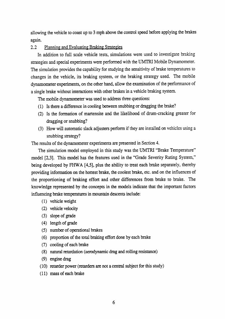
2.2 Planning and Evaluatiniz bra kin^ Strategie~
In addition to full scale vehicle tests, simulations were used to investigate braking
strategies and special experiments were performed with the UMTRI Mobile Dynamometer.
The simulation provides the capability for studying the sensitivity of brake temperatures to
changes in the vehicle, its braking system, or the braking strategy used. The mobile
dynamometer experiments, on the other hand, allow the examination of the performance of
a single brake without interactions with other brakes in a vehicle braking system.
The mobile dynamometer was used to address three questions:
(1) Is there a difference in cooling between snubbing or dragging the brake?
(2) Is the formation of martensite and the likelihood of drum-cracking greater for
dragging or snubbing?
(3) How will automatic slack adjusters perform if they are installed on vehicles using a
snubbing strategy?
The results of the dynamometer experiments are presented in Section 4. The simulation model employed in this study was the UMTRI "Brake Temperature"
model [2,3]. This model has the features used in the "Grade Severity Rating System,"
being developed by FHWA [4,5], plus the ability to treat each brake separately, thereby
providing information on the hottest brake, the coolest brake, etc. and on the influences of
the proportioning of braking effort and other differences from brake to brake. The knowledge represented by the concepts in the models indicate that the important factors
influencing brake temperatures in mountain descents include: (1) vehicle weight
(2) vehicle velocity
(3) slope of grade (4) length of grade (5) number of operational brakes (6) proportion of the total braking effort done by each brake
(7) cooling of each brake (8) natural retardation (aerodynamic drag and rolling resistance) (9) engine drag
(10) retarder power (retarders are not a central subject for this study)
(1 1) mass of each brake

Example sets of parametric data for representing the pertinent mechanical properties of
the UMTRI and NHTSA vehicles are presented in Appendix A. Example predictions of
brake temperatures on the Bragflandstone downgrade are also given in the Appendix A.
2.3 Vehicle Pre~aration, Vehicle preparations consisted primarily of (a) making sure the braking systems were
functioning properly; (b) loading the vehicles to the GCW's selected for the tests; (c) providing provisions for valve changes; and (d) instrumenting the vehicles.
The brake systems were thoroughly inspected. The linings had very little wear. The
brakes were adjusted. Preliminary testing of the vehicles included: (1) brake testing, including measurements of:
*brake timing (application and release times) *pressure balances (valve cracking and pushout pressures) *torque balances (chassis dynamometer tests) *stroke versus pressure without wheel rotation (and with wheel rotation)
*brake cooling rates at the control speed used in the mountain descents plus
cooling rates at zero velocity
(2) vehicle coast-down tests on a level surface to obtain measurements of parasitic drag ("natural retardation" and engine drag) with the clutch (a) engaged and (b)
disengaged.
(3) a stopping distance test from 45 mph on a good, level surface to demonstrate satisfactory braking capability.
The results of these tests assured that braking performance was normal and that there
were not any unusual properties that would influence brake temperatures in a strange
manner.
The UMTRI vehicle (see Figure 2) was loaded to 46,420 lb. to represent a heavily-
loaded straight truck. The tractor was loaded at its fifth wheel by the semitrailer.
However, the semitrailer's brakes were put on a separate braking circuit that was not used
in downhill testing. Hence, the UMTRI vehicle was operating like a heavily-laden straight
truck.
(The semitrailer's brakes were available for use as a safety measure in case the tractor's
brakes faded to the point that the driver felt that the truck was starting to runaway. It turned
out that the trailer's brakes were never needed in downhill testing. The semitrailer's brakes were connected to make a normal braking system for use in driving to and from the test
area.) The NHTSA vehicle was a three-axle tractor pulling a two-axle flatbed semitrailer. The
vehicle was loaded to 80,000 lb using cement blocks as shown in Figure 3. The

Figure 2. UMTRI Truck on tl
8
le Mountain

Figure 3. NHTSA 3-S2 Tractor-Semitrailer
tractor was equipped with a retarder for use in emergency situations. (No emergencies
arose and the retarder was only applied in a few runs to check its functionality.)
Both the UMTN and NHTSA tractors were "plumbed" so that different valves could
be employed to change the brake proportioning. The UMTN tractor had a front limiting
valve that could be introduced to reduce front braking effort. The NHTSA tractor had
high-flow, quick-release couplers between valves that could be used to change the braking
effort as indicated in Table 1. The vehicles were instrumented to measure:
(1) lining temperatures at each brake
(2) drum temperature at each brake
(3) brake chamber pressure at each axle or axle group (4) treadle pressure(s)
(5) velocity
(6) stroke at each brake
In addition, the NHTSA vehicle was equipped to measure stopping distance. (See
Appendix B for further information on the instrumentation. See Appendix C for more
information on the vehicles themselves.)

2.4 Conducting - the Test8 2.4.1 Background on Downhill Testing, The vehicles were driven to the
Bragg/Sandstone test site on 1-64 and the instrumentation and data gathering systems were
activated.
The plans for the downhill tests were based on an appreciation for the management of
the energy involved in descending a mountain. The total energy absorbed by the brakes
will depend upon the change in potential energy in descending the mountain. The change
in potential energy is equal to the weight of the vehicle multiplied by the change in elevation which is equal to the average slope multiplied by the length of the downgrade. For
example, the change in potential energy for the UMTRI truck descending the
Bragg/Sandstone mountain for 4 mi is equal to 58.5 million ft lb. If all of this energy were
to go uniformly into the brakes on the UMTRI truck, the change in average brake temperature would be approximately 1100° F. However, rolling resistance and engine drag might dissipate 20 to 30 million ft lb, resulting in maximum average temperature changes of
approximately 700' F to 500' F. In addition, the brakes are also cooling during the descent such that in practice the maximum average temperature change turned out to be
approximately 380' F at the bottom of the mountain for the UMTRI truck. Natural retardation from the rolling resistance of the tires and other sources of rolling
resistance is equal to approximately 1 to 1.5 percent of the weight. (It is like a 1 to 1.5
percent reduction in grade.) The engine provides additional retardation if the clutch is engaged. For a given speed down the hill, the driver should pick a gear that will result in
an engine speed near rated speed. This will provide a much higher level of engine drag than that which would be obtained if the driver had picked a gear that resulted in a low
engine speed. It is important that drivers understand that the use of a high engine speed
and a low vehicle speed is the way that they can control brake temperatures. Altogether
rolling resistance, engine drag, and aerodynamic drag may provide the equivalent of a 2
percent reduction in grade for speeds above 30 mph. At lower speeds, aerodynamic drag is
small and the natural retardation will amount to less than 2 percent. (These numbers are
approximations for new fuel-efficient vehicles and further advances in fuel economy will mean even less natural retardation.)
Given an appreciation for the need to allow enough time for the brakes to dissipate heat,
the first order of business after getting the vehicle ready was to determine the proper control speed for descending the mountain. The speed needs to be slow enough for sufficient
energy to flow from the brakes to keep brake temperatures Erom rising too much. If the

vehicle is driven too rapidly, the brakes will overheat since too much energy will be stored
in the brakes and not enough energy will have been dissipated from the brakes.
Preliminary runs down the mountain were made with the UMTRI vehicle at 25 mp h,
then 30 mph, and finally, 36 mph. Temperatures less than 600' F were achievable at 36
mph, and 36 rnph was chosen as the control speed for the UMTN vehicle.
Preliminary runs down the mountain were made at 25 rnph with the NHTSA vehicle.
High temperatures approaching 1000° F were recorded on some brakes and smoking was
observed before the bottom of the mountain was reached. Due to the proportioning of
braking effort on the NHTSA vehicle, the trailer brakes did more than their fair share of the
work. The initial control speed of 25 rnph was reduced to 20 rnph later.
These control speeds meant that the UMTRI vehicle took approximately 400 sec in
descending the mountain and the NI-l[TSA vehicle took almost 800 sec.
After descending the mountain, the vehicles were driven several miles to the next
interchange after Sandstone to provide time for the brakes to cool. By the time the UMTRI
vehicle had gone to the next interchange, turned around, and climbed to the top of the
mountain again, its brakes were cooled to 150' F or less. The vehicle was ready for
another test. The initial brake temperatures were low enough. Due to the high temperatures of some of the brakes of the NHTSA vehicle, further
driving was often needed to reach brake temperatures less than 150' F.
Basic equations explaining the influences of vehicle speeds and time periods on brake
temperatures are presented in Appendix D. The idea behind the equations is to describe the heat flow into and out of the brakes. The equations show that if the mountain is long and
steep enough (that is, the potentid energy change is large) and the vehicle speed is great enough, the brakes will overheat. This is because the heat flow out of the brakes (i.e., the
cooling) will not have enough time to dissipate the heat absorbed by the brakes. Travelling at a lower speed will allow more time for the brakes to cool and the vehicle will reach the
bottom of the mountain at lower brake temperatures. In driving without braking, higher speed will increase the heat flow from the brakes
and allow them to cool quicker. (Even though one has to drive further to lower the
temperature by the same amount, it will be quicker to drive faster.)
2.4.2 Mobile Dynamometer Studies, The UMTRI mobile dynamometer was used
to study a single brake. The brake was installed in the tire-wheel assembly located centrally
on the test trailer of the mobile dynamometer (see Figure 4).
Instrumentation was provided in the dynamometer to measure brake torque, wheel
speed, vertical load, and braking force. The brake was instrumented to measure pressure,
drum and lining temperatures, and stroke (much as was done for the vehicle tests).

Figure 4. UMTRI Mobile Dynamometer

The first series of mobile dynamometer tests involved simulated mountain descents.
The dynamometer was driven at 30 rnph to represent a typical control speed. Snubbing and
dragging strategies were used for periods of approximately 400 to 500 sec to represent long grades. The level of brake torque was controlled to simulate the amount of work done by
the brake in a mountain descent. These tests were used to study the influences of braking
strategies on cooling rates. Another set of mobile dynamometer tests was used to study the influences of braking
strategy on "hot-spotting" of brake drums. For these tests, the mobile dynamometer was driven at 60 mph and the brakes were applied (either snubbing or dragging) for one minute.
These tests simulated speed control on mild rolling hills. Areas of hot-spotting were
measured on the dnuns after 100 of these simulated tests, starting with green linings.
Finally, a limited study of the influence of the snubbing technique on the performance
of one type of automatic slack adjuster was performed using the mobile dynamometer. The
dynamometer was used to simulate mountain descents at 40 mph with a snubbing strategy
consisting of cyclic applications of the brake involving 3 see of braking at approximately 20
psi and then 6 sec off. These duty cycles of braking were continued for approximately 340
sec until the drum temperature ieached approximately 600' F. Brake pressures and strokes
were measured before and after four simulated mountain descents to determine if the
snubbing strategy had disrupted the functioning of the automatic slack adjuster.
3 . 0 RESULTS FROM DOWNHILL TESTS OF COMPLETE VEHICLES
3.1 ksul t s for the UMTRI truck,
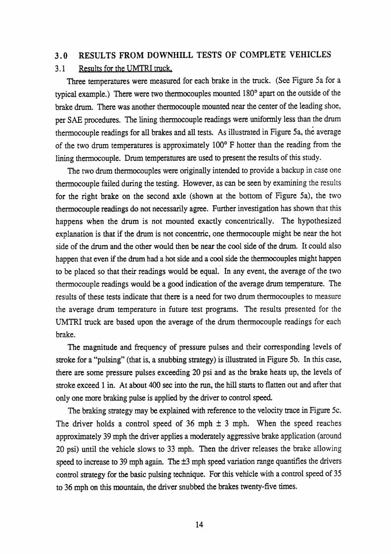
Three temperatures were measured for each brake in the truck. (See Figure 5a for a
typical example.) There were two thermocouples mounted 180' apart on the outside of the
brake drum. There was another thermocouple mounted near the center of the leading shoe,
per SAE procedures. The lining thermocouple readings were uniformly less than the drum
thermocouple readings for all brakes and all tests. As illustrated in Figure 5a, the average
of the two drum temperatures is approximately 100' F hotter than the reading from the
lining thermocouple. Drum temperatures are used to present the results of this study.
The two drum thermocouples were originally intended to provide a backup in case one
thermocouple failed during the testing. However, as can be seen by examining the results for the right brake on the second axle (shown at the bottom of Figure 5a), the two
thermocouple readings do not necessarily agree. Further investigation has shown that this happens when the drum is not mounted exactly concentrically. The hypothesized
explanation is that if the drum is not concentric, one thermocouple might be near the hot side of the drum and the other would then be near the cool side of the drum. It could also
happen that even if the drum had a hot side and a cool side the thermocouples might happen to be placed so that their readings would be equal. In any event, the average of the two
thermocouple readings would be a good indication of the average drum temperature. The
results of these tests indicate that there is a need for two drum thermocouples to measure
the average drum temperature in future test programs. The results presented for the
UMTRI truck are based upon the average of the drum thermocouple readings for each brake,
The magnitude and frequency of pressure pulses and their corresponding levels of stroke for a "pulsing9' (that is, a snubbing strategy) is illustrated in Figure 5b. In this case,
there are some pressure pulses exceeding 20 psi and as the brake heats up, the levels of
stroke exceed 1 in. At about 400 sec into the run, the hill starts to flatten out and after that
only one more braking pulse is applied by the driver to control speed
The braking strategy may be explained with reference to the velocity trace in Figure 5c.
The driver holds a control speed of 36 mph f 3 mph. When the speed reaches
approximately 39 mph the driver applies a moderately aggressive brake application (around
20 psi) until the vehicle slows to 33 mph. Then the driver releases the brake allowing
speed to increase to 39 mph again. The f 3 mph speed variation range quantifies the drivers
control strategy for the basic pulsing technique. For this vehicle with a control speed of 35
to 36 mph on this mountain, the driver snubbed the brakes twenty-five times.

Figure 5a. UMTRI Truck Pulsing Test

Brake tine Pressure, Axle 2 - PSI 40
30
a
10
0
0 290 400 6#] 800
Tim sac bhad8adrb3, ~ 3 S M P H ; T d I o e B L P a m r f i i t ~
Figure 5b. UMTRI Truck Pulsing Test (continued)

Pressure - PSI (Both lines at the treadle valve)
40
Figure 5c. UMTRI Truck Pulsing Test (continued)
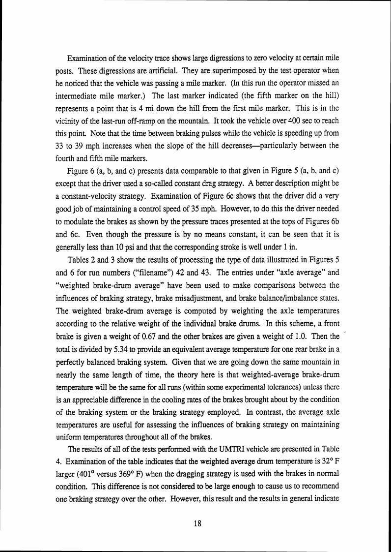
Examination of the velocity trace shows large digressions to zero velocity at certain mile
posts. These digressions are artificial. They are superimposed by the test operator when he noticed that the vehicle was passing a mile marker. (In this run the operator missed an intermediate mile marker.) The last marker indicated (the fifth marker on the hill)
represents a point that is 4 mi down the hill from the first mile marker. This is in the vicinity of the last-run off-ramp on the mountain. It took the vehicle over 400 sec to reach this point. Note that the time between braking pulses while the vehicle is speeding up from 33 to 39 mph increases when the slope of the hill decreases-particularly between the
fourth and fifth mile markers.
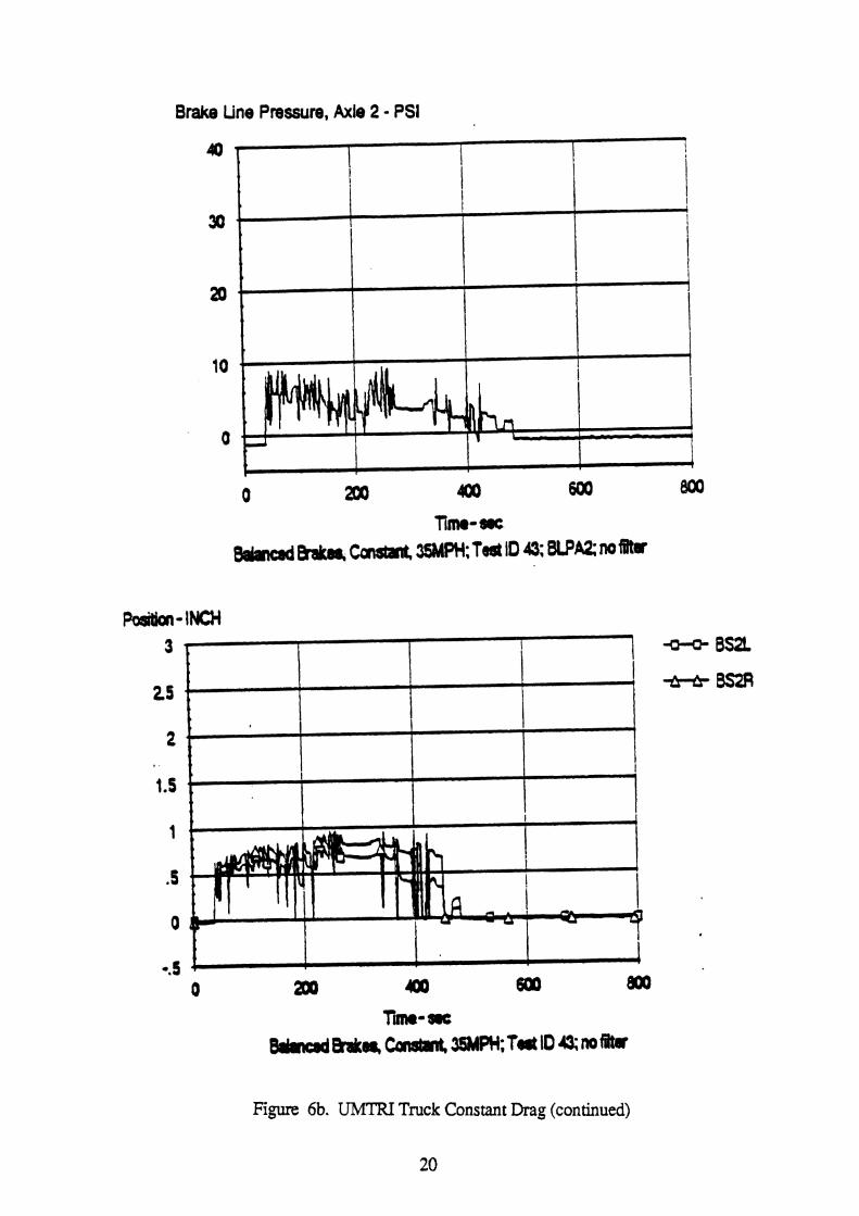
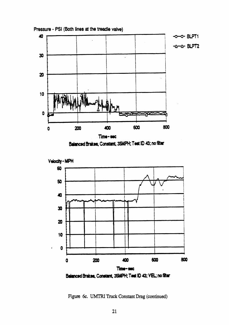
Figure 6 (a, b, and c) presents data comparable to that given in Figure 5 (a, b, and c)
except that the driver used a so-called constant drag strategy. A better description might be
a constant-velocity strategy. Examination of Figure 6c shows that the driver did a very
good job of maintaining a control speed of 35 mph, However, to do this the driver needed
to modulate the brakes as shown by the pressure traces presented at the tops of Figures 6b
and 6c. Even though the pressure is by no means constant, it can be seen that it is
generally less than 10 psi and that the corresponding stroke is well under 1 in.
Tables 2 and 3 show the results of processing the type of data illustrated in Figures 5 and 6 for run numbers ("filename") 42 and 43. The entries under "axle average" and
"weighted brake-drum average" have been used to make comparisons between the
influences of braking strategy, brake misadjustment, and brake balance/imbalance states.
The weighted brake-drum average is computed by weighting the axle temperatures
according to the relative weight of the individual brake drums. In this scheme, a front
brake is given a weight of 0.67 and the other brakes are given a weight of 1.0. Then the '
total is divided by 5.34 to provide an equivalent average temperature for one rear brake in a
perfectly balanced braking system. Given that we are going down the same mountain in
nearly the same length of time, the theory here is that weighted-average brake-drum temperature will be the same for all runs (within some experimental tolerances) unless there is an appreciable difference in the cooling rates of the brakes brought about by the condition
of the braking system or the braking strategy employed. In contrast, the average axle
temperatures are useful for assessing the influences of braking strategy on maintaining uniform temperatures throughout a l l of the brakes.
The results of all of the tests performed with the UMTRI vehicle are presented in Table 4. Examination of the table indicates that the weighted average drum temperature is 32' F
larger (401' versus 36g0 F) when the dragging strategy is used with the brakes in normal
condition. This difference is not considered to be large enough to cause us to recommend one braking strategy over the other. However, this result and the results in general indicate

Figure 6a. UMTRI Truck Constant Drag
Brake Line Pressure, Axle 2 - PSI
Figure 6b. UMTRI Truck Constant Drag (continued)
Pressure - PSI (Both lines at the treadle vatve) 413
Figure 6c. UMTRI Truck Constant Drag (continued)


Table 3. Brake Tem~eratures and Strokes for File 43 FILENAME: 43 I
I
BS3R I 0.58 1 49 1 Average Pressure from 50 to 375 sec
I ,TITLE: Balanced Brakes, Constant Drag, 35MPH, 6th Gear High, Rear Brakes 1.25 Stroke Average Velocity figured from 50 to 375 sec: 35 Brake Lining Temperature from 50 to 450 sec
Name BLPT1 BLPT2 BLPA1 BLPA2 BLPA3
Name LINER-1 L LINER-1 R LINER-2L
Average 6.8 6.0 6.5 5.5
. 5.5
Peak 110 304 31 3
Time 381 370 371

Table 4. Summarv of UMTRI Results
29
3 3
that pulsing is as good as dragging (or even slightly better) with regard to maintaining the
42
48
34
4 1
44
3 5
40
45
3 7
47
overall level of brake temperature for this vehicle. From an overall standpoint, the brakes
normal 6 6
absorb approximately the same proportion of the potential energy due to the mountain
1 4
6 6
misadjustment 66
66
misadjustment 6 1
6 6
normal 6 6
regardless of the strategy used, the level of adjustment, or the pressure balance of the
pulse 6 6
brakes.
6 6
6 1
pulse 6 6
6 6
drag 6 6
6 6
exaggerated snub 6 6
35 1
366
373
386
383
397
367
385
374
375
378
367
369 #3,389
382
378
372
#2,394
#2,400
#3,389

Inspection of Table 4 indicates that there are differences between the maximum (peak)
temperatures from axle to axle. The largest difference occurs when a front limiting valve is
used. This is because the front brakes do almost nothing when the limiting valve is
employed. The temperature differences from axle to axle are more readily understood
when they are plotted for each axle as in Figures 7 through 10. These results show that pulsing tends to result in more uniform temperatures from brake to brake. Even in the case
of a front limiting valve (see Figure lo), the pulsing strategy results in the front brakes
doing a little work as indicated by a slight temperature rise. From the uniformity of
temperature standpoint, pulsing is definitely a better strategy than dragging but the results
are not dramatic for this vehicle.

Change in Drum Temperature Baseline
a Run 3 1 Drag
+ Run 32 Drag
A Run 43 Drag
-0 Run 49 Drag
.+ Run 29 Pulse
A Run 33 Pulse
.+. Run 42 Pulse
+ Run 48 Pulse
200 --
100
0
--
I I I
Figure 7. The Influence of Braking Strategy for the Truck
Axle 1 Axle 2 Axle 3
m
200
100
0
-- 4 Pulse Average
-- 0 Drag Average
I I I Axle 1 Axle 2 Axle 3

Change in Drum Temperature Misadjusted Brakes
0 Axle 1 Axle 2 Axle 3
Run 35 Drag
O. Run 40 Drag
b Run 45 Drag
C Run 34 Pulse
IC Run 41 Pulse
* Run 44 Pulse
a Pulse Average
Drag Average
0 ! I I I
Axle 1 Axle 2 Axle 3
Figure 8. The Influence of Misadjustment for the Truck
27
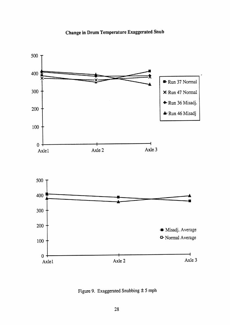
Change in Drum Temperature Exaggerated Snub
0 Axle 1 Axle 2 Axle 3
* Run 37 Normal
Xm Run 47 Normal
C Run 36 Misadj.
A Run 46 Misadj
Figure 9. Exaggerated Snubbing f 5 mph
200
100
0
-- .~c Misadj. Average
-- * Normal Average
I I I
Axle 1 Axle 2 Axle 3

Change in Drum Temperature Front Limit Values
+ Run 38 Drag
t Run 39 Pulse
Axle 1 Axle 2 Axle 3
Figure 10. The Influence of a Front Limit Valve on Brake Temperatures
3.2 Results for the NHTS A tractor semitrailer (3-S22 This vehicle also performed tests using both drag and snub strategies. Figures 11 and
12 provide examples of results. As illustrated in Figure 9, the constant-drag strategy
produced a wide diversity in temperatures from brake to brake. The brake temperatures
were much more uniform when the pulsing (snubbing) strategy was used (see Figure 12).
As indicated in these figures, the trailer brakes reached high temperatures. When the temperatures were quite high, the strokes became long-over 2 in when snubbing was
used. These results were obtained even though the control speed was at 20 mph in these runs. Almost 800 sec were needed to reach the bottom of the mountain.
The runs from the 3 4 2 tractor semitrailer have been processed for weighted average
temperature (see Figure 13). For this vehicle it appears that the dragging strategy maintains
lower temperatures in most cases. However, these differences are usually small and
sometimes the snubbing strategy is better. We do not consider the differences to be
grounds for recommending one strategy over the other. In fact, if some brakes get very hot they will cool more due to radiation, and this additional cooling may lead to a lower overall
weighted temperature.

When the constant-drag method was employed, the brakes on the tractor's drive axles of the 3-S2 did very little braking, as indicated by the low temperatures appearing for
the drive axles in Figure 14. Balance level B was particularly bad in this regard because the
threshold pressure was 12.1 psi (see Table 1). In contrast, when the pulsinglsnubbing
strategy was used, the drive-axle brakes did an appreciable amount of the braking and the
temperatures attained at the trailer's axles tended to be noticeably lower than those attained
when a dragging strategy was used. As in the case of the truck, the pulsing strategy
produced a more uniform distribution of brake temperatures and each brake came closer to
doing its fair share of the work.

Tcoc tor 0-wn Temps Q\ 20 be1 odj
lW.*
0. t I 1 I I
0. loo. PO. YO. #. 00.
TYms (see)
0. " I I I I i d. 10. PO. *). W. m.
Troller Strokes - b 20 bol odj
t i m e (sac) T i n (see)
Figure 1 1. NHTSA 342 Constant Drag

T r o c t ~ b Temps - Snk 20 bal odj 1OQO.
0. I 1 I 1 I i 0. 1m. PO. UQ. m. (00.
Tim (see)
0. 1 I
0. a. . i. . I T i m e (set)
Trailer Strokes - St?& 20 bal odj
/ Oist ( x l w ) - S& 20 bal odj
="**
Figure 12. NHTSA 342 Pulsing Test

Downhill Braking Tests M B r b Adjusted
600 I
Figure 13. Weighted Average Drum Temperatures (3-S2)

Downhlll Braklng Tests Balancs Level A, Adjusted Brakes, 20 & 25 mph
1
f '*: + Snub Method + Drag Method I ,
o O ~rbnt Drive Traller Me(s)
Balance Level 8, Adjusted Brakes, 20 & 25 mph
+ Snub Mettwd 1 Front Drtve Traller
Balance Level C, Adjusted Brakes, 20 mph @so0
1:: c 400
;: r: +Snub Method ' -c Drag Method
orhn Trailer Me(r1
Figure 14. Average Temperatures by Suspension Grwp (342) The Influence of Balance Level

Figure 15 provides results obtained when the drive axles7 brakes are set to have an
applied stroke of 2 in at 100 psi. (This did not change the temperatures much-partially
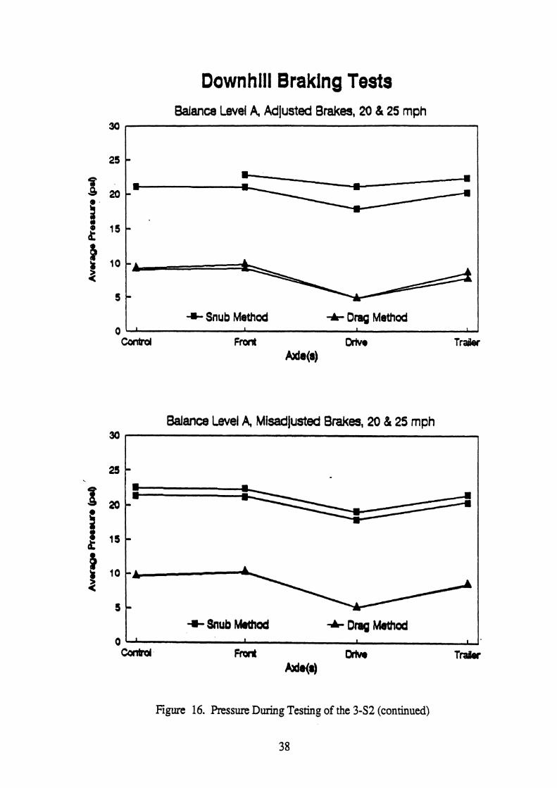
because the drive-axle brakes did a limited amount of the total braking on this vehicle.) Figure 16 gives an indication of the pressure levels used during the braking tests. The
low level of pressure at the drive axles is apparent for the constant drag strategy.
The NHTSA vehicle was equipped to obtain stopping distance measurements. Stopping distance tests were performed on a nearly level section of highway at the bottom of the mountain. These tests were from an initial velocity of 35 mph using 60 psi brake pressure. A complete set of results is presented in Table 5.
The results in Table 5 run from a minimum of 89 ft to a maximum of 130 ft (which
correspond to deceleration levels of 0.46 g and 0.32 g, respectively). The differences in
stopping performance may be related to (a) control speed and (b) whether the brakes are
misadjusted.
For those runs at 25 mph in which the brakes were not misadjusted, the distances were
longer than the comparable runs at 20 mph. This is to be expected since the brake
temperatures were higher at 25 mph than they were at 20 mph. The influence of
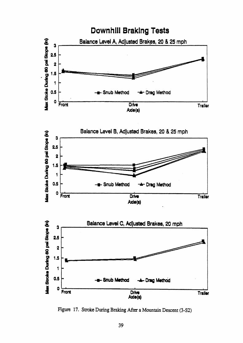
temperature on drum expansion and hence stroke is illustrated in Figure 17, which shows
stroke during the 60 psi stops.
The last graph on the second page of Figure 17 shows the strokes at each suspension
location for cases with misadjusted brakes. Examination of this graph for misadjusted
brakes indicates that the stroke is beyond the readjustment point and well into the range
where braking force will be considerably reduced at 60 psi for both the drive-axle and the
trailer axle brakes. The stroke is large at the drive-axle brakes because they are
misadjusted. The stroke is large at the trailer brakes because they are very hot. The
combination results in poor braking performance for those runs in which rnisadjustment
appears (runs e, f, k, 1, o, and p in Table 5). The results for runs o and p indicate that, under conditions of (a) misadjusted brakes on
the tractors drive axle and (b) pneumatic balance that reduces the relative amount of work
done by the front axle brakes (i.e., Case C), a longer stopping distance was measured after
snubbing as compared with dragging the brakes. However, it is not fair to compare runs o
and p because in the dragging run p the trailer brake temperature became large enough to
cause the driver to stop using the foundation brakes. The net effect was an incremental increase in stopping distance after the snubbing test.

Down hlll Braklng Tests Balance Level A, Adjusted Brakes, 20 & 25 mph
000
0 Ftont
0
- + Snub Method -.lc Drag Method
I I I
Balance Level A, Mlsadjusted Brakes, 20 & 25 mph 800
-
- .. 0
o + Snub Method 4 Drag Method
I 1 1 0 Ftont
Figure 15. The Influence of Misadjustment on the 342

Downhlll Braklng Tests 30
Bahncr Level A Adluaed Brakga, 20 & 25 mph
I -a- Snub Mettrod + Drag Mettrod Odaiml
J Fmnt Dtive Trailer
Balance Level 8, Adjusted %ekes, 20 & 25 rnph 30 1
~dkmd 1 hont D r h Trader
+ Snub Mathod -t Drag Method
Balancs Level C, Adfusbd Brakw, 20 rnph 30
I I
Front Dm Tdof
Figure 16. Pressure During Testing of the 342
Downh111 Braklng Tests Balance Level A, Adjusted Brakes, 20 & 25 mph
30 i
I
-
I)
+ Snub Method -+ Drag Method I I I I
Balance Lev4 A, Mlsadjwted Brakes, 20 & 25 mph 30
Figure 26. Pressure During Testing of the 3 4 2 (continued)
Downhill Braking Tests
2 Balance Level 8, Adjusted Brakes, 20 & 25 rnph
i 3
$ 3 9 Balance Level A, Adjusted Brakgg, 20 I% 25 rnph
O*" -c Snub Method i. Drag Mattrod
4 OFA 0 t h Traller MQ(~)
Bas II 2 - 8 * p l " - d l -
f 3 Balance Levd C, Adjusted Brakes, 20 mph
1 2."-
4
1 2 -
1 -
-
-t Snub M o d + Drag Mahd
-.- Snub Math4 -+. Drag Method
. Or tva Traller
Me(a)
# Lrh o r b trailer 1 Mda)
Figure 17. Stroke During Braking After a Mountain Descent (3-52)

Down hlll Braklng Tests
BaJanc8 Level A, Misadiusbd Brakes, 20 & 25 mph 3 I
Balance Level A, Adlusted Brakes, 20 & 25 rnph
Figure 17. Stroke During Braking Afta a Mountain Descent (342) (continued)
3
a 2.5
P 8 2
i " 1 8 1
8 0.5
S
- -
- + Snub Method + Olag Method

Table 5. 3 4 2 Stopping Distances Attained in 60 psi Stops from 35 mph After
"g aborted after descending 314 of the mountain
Aside from the circumstances associated with balance level C, the influence of
snubbing versus dragging on stopping distance was small. Key factors for producing
longer stopping distances are (1) misadjusted brakes on the tractor combined with
pneumatic balance that will produce very hot trailer brakes (of course, the same result could
be obtained with misadjusted trailer brakes combined with a pneumatic balance that
produced very hot brakes on the tractor) and (2) the control speed used in descending the
mountain.

4 . 0 RESULTS FROM MOBILE DYNAMOMETER TESTS OF INDIVIDUAL BRAKES
4.1 cool in^ rates for d ru ing : and snubbin? strate@es,
The first set of mobile dynamometer experiments provided data for use in comparing
cooling rates for dragging and snubbing strategies. In these experiments, the mobile dynamometer was traveling at 30 mph to simulate a mountain-descent control speed of 30
mph.
The brake under test was applied at a constant torque of 8,000 in lb to simulate a
constant dragging strategy. This torque was applied for a sufficient length of time
(approximately 400 sec) to raise the average outside drum-temperature to over 600" F. (See
Figure 18 for examples of time histories of data from a typical experimental run simulating
the dragging strategy on the mobile dynamometer,)
To simulate a snubbing (also referred to as "pulsing") strategy, the brake was applied in
"pulses" of torque reaching approximately 24,000 in lb. (See the brake-torque tirne-history
in Figure 19) Since the pulses last for about 3 sec followed by 6 sec with no braking, the
average torque during pulsing was approximately the same as the constant torque used in
the dragging experiments.
The data obtained from four repeats of the drag test and four repeats of the snub (pulse)
test have been analyzed to estimate the cooling rates of the brake during the experimental
runs. The analysis procedure is based upon the physical model of heat flow presented in
Appendix D. The computation of cooling rate involves calculating two integrals from the
time histories of the test data. The work done by the brake (i.e., the energy absorbed by
the brake) is the integral of the product of brake torque times rotational speed. The other
integral computed in processing the data is the integral of brake drum temperature. Using
these two integrals (and also data on the initial and final drum temperatures and braking
times; and values for ambient temperature, specific heat, and drum mass), the experimental
data can be used to determine the cooling rate while braking is occurring. The results are presented in Table 6.

7 - - -
0 200 400 600 , 800
Time - sec Type A Liners; Constant Drag; Test ID 37; VEI; no fitter
B. Temperature - DEGF
-0--CI- DRUM1
* DRUM2
Time - sec Type A Liners; Constant Drag; Test ID 37; Lopass = 5
Figure 18. Cooling Rate Experiment, Drag Test

E. Brake Stroke - INCH
Figure 18. Cooling Rate Experiment, Drag Test (continued)
44
-5 f
0 .,s
-.5
-1
-1.5
-2
-2.5
-3 b
0 200 400 600 800
Time - sec Type A Liners; Constant Drag; Test ID 37; BAP; no filter

C. Brake Torque - IN-LBS
Time - sec Type A Unen; Constant Drag; Test ID 37; TB; no fitter
D. Brake Line Pressure - PSI
Figure 18. Cooling Rate Experiment, Drag Test (continued)
30
20
10
.=
a -
*.
0 -
b
0 200 400 600 800
Time - sec Type A Liners; Constant Drag; Test 10 37; BLP; no filter

A Vekcity- MPH
60
0 200 400 600 800
Time - sec Type A Linen; Pulsed Brakes; Test ID 38; VEk no filter
B. Temperature - DEGF
Time - sec Type A Uners: Pulsed Brakes; Ted ID 38; Lopass = 5
Figure 19. Cooling Rate Experiment, Snub Test

C. Brake Toque - IN-LBS
0 200 400 600 000
Time - sec Type A Liners; Pulsed Brakes; Test ID 38; TB; no fitter
D* Brake Line Pressure - PSI
0 200 400 600 800
Time - sec Type A Liners; Pulsed Brakes; Test ID 38; BLP; no filter
Figure 19. Cooling Rate Experiment, Snub Test (continued)

E. Brake Stroke - INCH
Time - sec Type A Liners; Pulsed Brakes; Test 10 38; BAP; no filter
Figure 19. Cooling Rate Experiment, Snub Test (continued)
48

Table 6. Mobile Dvnamometer Cooling Rate Ex~eriments. 30 m ~ h
11 DRAG: 11
11 SNUB: 11
* This was taken from one thermocouple.
THf - Final temperature, O F THi - Initial temperature, OF tf- Final time (braking ends), sec ti- Initial time (braking starts), sec Energy - Total work done by the brake, ft lb IntTH - Integral of brake temperature from ti to tf, O F see H3o - Cooling rate at 30 mph, ft lb/ O F sec
Conditions used in analysis: -
H = Energy - mcp(THf - TH;) THa - ambient temperature: 80 OF
m - weight of heated mass: 100 lb I I. TH dt - THa (trti)
cp - Specific heat: 100 ft lb/ lb O F d
Cooling rates at 30 mph:
H30, drag average: 12.9 ft 1bJ lb ?F
H30, snub average: 15.3 ft 1bJ Ib OF (14.8 without file 40)
Examination of the results in Table 6 indicates that the estimated cooling rate for the
pulsing strategy was 15.3 ft lb compared to 12.9 ft lb for the dragging strategy. Tsec Tsec

According to these results, at the same average rate of doing work, it will take longer
for the brake to heat up using the snubbing strategy than it does using a dragging strategy.
However, the difference in cooling rate is not large. (It is approximately 15 percent larger
for the snubbing strategy.) The difference in cooling rate might appear to be large enough
to cause observable differences in temperature in practice, but it did not appear to be an
important factor in the downhill tests. In practice on an actual vehicle with several brakes
with various levels of proportioning and effectiveness, the cooling advantages of pulsinge
the brakes were not large enough to be noticed.
4.2 artensite and drum discolorization,
The mobile dynamometer was also used to simulate descending a short mountain (one
mile downgrade) for one minute at 60 mph. Both pulsing (snubbing) and dragging
strategies were used at an average torque level of 5,300 in lb. In the snubbing case, the
duty cycle consisted of 3 sec of brake application at 15,900 in lb followed by 6 sec of no braking. In the dragging case, a constant torque level of 5,300 in lb was maintained. Each
simulated descent was followed by 10-15 min of no braking, allowing the brake to cool
rapidly.
Two types of linings designated A and B were used. The lining designated A is a very common type of lining often used as original equipment. The B was chosen because it was known to be prone to promoting martensite formation by Mr. Anderson who is an expert in
drum-cracking [6]. Four drums were required for the combination of two strategies with two types of linings.
Results were obtained for one hundred repetitions of the mountain descent simulation starting with new (green) linings. In addition, results were also obtained after 150 repetitions in the worst case which was the drag strategy using the B lining.
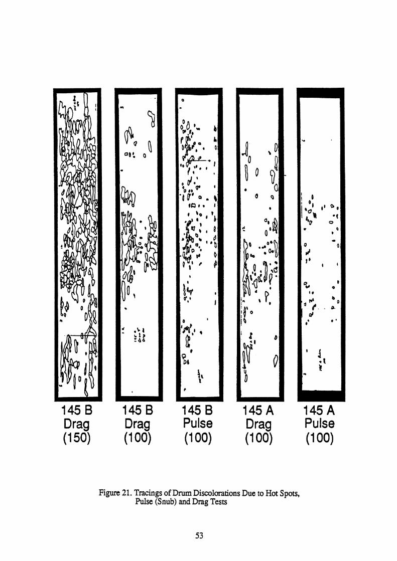
The results are expressed in terms of the amount of rubbing surface area that showed color change due to the formation of hot spots. Figure 20 provides an idea of the information that was recorded through a careful examination of the inside surface of the brake drum. To obtain a rough comparison between the results for different test conditions
(drag versus pulse and A versus B), the areas of color change were traced onto vellum and
measured (See Figure 21). Based upon a rubbing surface area of 389 in2 (250,900 rnm2), Table 7 presents results showing that after 100 simulated descents, the Alpulse case had the
least martensite formation. If dragging were used instead of pulsing, the amount of
discolored area increased seven times with the A lining. The B lining produced much
worse results and the B/drag case was eleven times worse than the A/pulse case after 100
discolored for the B/drag case. Evidence in the literature [5] indicates that drum failure may

Figure 20. "3 O'clock" and "9 O'clock" Views of Brake Drums


Figure 20. "3 O'clock" and "9 O'clock" Views of Brake Drums (continued)
52

. oDO )" r * 3,.
1, y:* fl
@. iy;* 4 1 I
8 dl ' 0 0 ' ' 0 4;
'00' 0 \! t R 8 r I
: pa: " b
0 1 , 4 '
* I+ l
0.I ' I
0 I
i ~ ' , l , I?
0 Q Dt
t
b
145 B 145 6 145 B 145 A 145 A Drag Drag Pulse Drag Pulse (1 50) (1 00) (100) (1 00) (1 00)
-
Figure 21. Tracings of Drum Discolorations Due to Hot Spots, Pulse (Snub) and Drag Tests
Y
I ! 0
O I (I * ( j b O I I
3, 0 w 0
b
0
0 0 d 1' , ,
Pu 0 0 ' e
d r' 0 f . . a.
d 8'
* *
' 1 * i t
i !
I

result soon if martensite formation continues to develop through dragging. The clear
implication of these experimental results is that the snubbing strategy is much better than
the dragging strategy when it comes to reducing the formation of hot spots.
Table 7. Martensite Formation/Drum Discoloration I I
4.3 The influence of ~ulsing on an automatic slack adiuster.
There has been concern that automatic slack adjusters might overadjust when a pulsing
strategy is used with hot brakes. After the brake cools, the brake would drag if it had been
overadjusted. This subsection presents data showing how one common type of automatic slack adjuster (a force sensitive type) performs during repeated brake applications involving the snubbing strategy.
The automatic slack adjuster was set to start with an initial adjustment of 2 inches of stroke at 80 psi brake pressure. (The characteristics of stroke versus pressure for the initial
state of the brakelslack adjuster combination are shown at 5, 10,20,40, and 80 psi along
with a gradual "sweep" of pressure from 0 to 80 psi in Figure 22.) This initial state of adjustment is at the readjustment point according to Federal Motor Carrier Safety Standards (that is where brake penalties for out of adjustment begin). Given this state of adjustment, the automatic slack adjuster is expected to reduce the stroke at 80 psi.
Number of
Simulated Descents
100
100
Case
Atpulse Bl~ulse
Discoloration
(m2) 1,880
9.840
% rubbing surface
area
0.8
3.9

Brake tine Pressure - PSI 100
20 40 60 80
Time - sec Auto Slack Test; Test ID 115; BLP; no fitter
Brake Stroke - INCH 2.5
20 40 60 80
7me - sec Auto Slack Test; Test ID 1 15; HAP; no filter
Figure 22. Pressure and Stroke for First Auto Slack Test

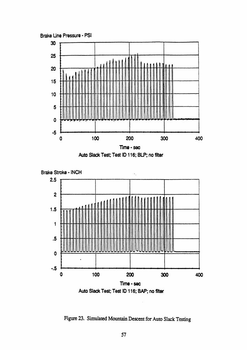
After a simulated mountain descent at 40 mph and of sufficient duration for the average
drum temperature to exceed 600° F (this involved 36 snubs at approximately 25,000 in lb,
see Figure 23), the cold stroke at 80 psi measured 1.75 in. After performing another
similar mountain descent, the cold stroke at 80 psi measured 1.6 in. After a third descent,
the cold stroke did not change fiom that attained after the second simulated mountain
descent, 1.6 in. Figure 24 shows the stroke versus pressure data after the third descent,
and comparison of these data with those presented in Figure 22 shows that the automatic
slack adjuster is performing as it should. The snubbing strategy and the high temperatures
involved did not adversely affect the performance of the automatic slack adjuster.
Brake Line Pressure - PSI 30
lime - sec Auto Slack Test; Test ID 1 16; BLP; no filter
Brake Stroke - INCH 2.5
1 00 200 300
Time - see Auto Slack Test; Test ID 1 16; BAP; no filter
Figure 23. Simulated Mountain Descent for Auto Slack Testing
57

Brake Torque - IN-US 5000
Time - sec Auto Slack Test; Test ID 1 16; TB; no fiiter
Figure 23. Simulated Mountain Descent for Auto Slack Testing (continued)
5 8

Brake Stroke - INCH
Brake tine Pressure - PSI
Time - sec Auto Slack Test; Test ID 121 ; BAP; no filter
100 -
8 0 .
6 0 .
40
20
Figure 24. Stroke and Pressure After the Third "Descent"
0 . " iT I
-20 +
0 20 40 60 80 100
Tme - sec Auto S W Test; Test .ID 121 ; BLP; no filter
I
I I
I I
.- 1 I I
-.
m

5.0 SUMMARY OF FINDINGS, CONCLUSIONS, AND RECOMMENDATIONS.
The findings from the mobile dynamometer experiments, described in Section 4,
indicate the following: *The snubbing (pulsing) strategy provides a higher cooling rate than that provided by
the dragging strategy. However, the difference is not large.
*The dragging strategy is more conducive to the formation of hot spots than the snubbing strategy when new linings are installed
*The use of a snubbing strategy for mountain descents will not cause a common type of
automatic slack adjuster to perform improperly. These findings all support the use of the snubbing strategy. The findings from the
mountain descent testing , described in Section 3, indicate the following:
*The overall level of brake temperature per pound of brake drum will be nearly the same
regardless of whether a constant dragging or a snubbinglpulsing strategy is used. The
test data did not indicate that one strategy provided significantly better cooling than the
other.
*The snubbing strategy involves higher pressures than the dragging strategy and
thereby tends to provide a more uniform temperature distribution from brake to brake
and from axle to axle. Through this mechanism, the snubbing strategy aids in making
each brake do its fair share of the work even if there is a gross pneumatic imbalance.
*Very high brake temperatures result if some brakes are not doing much work.
Tractors and trailers need to be matched through pressure and temperature balances if
high temperatures are to be avoided in mountain descents. (The grade severity rating
system is not conservative in this respect since it lumps all of the brakes together as if
each brake were doing approximately a fair share of the work.)
*Significant losses in stopping capability can be attributed to misadjustment combined
with pneumatic imbalance. Particularly poor stopping performance will occur after
mountain descents when the tractor's brakes are misadjusted and the trailer's brakes are very hot due to pneumatic imbalance, or vice versa with hot tractor brakes due to pneumatic imbalance and the trailer's brakes misadjusted.
*In some circumstances, with combined misadjustment and imbalance, the snubbing strategy has been found to lead to hotter brakes for the misadjusted brakes, which in turn leads to an additional increment in stopping distance after a mountain descent.
The findings from the mountain descent tests favor the snubbing strategy in that the hottest brake will be cooler if snubbing is used rather than dragging. However, the
differences in average brake temperature are not large enough or consistent enough to favor

either strategy. The snubbing strategy appears to have an advantage over the dragging
strategy because the snubbing strategy causes each brake to come closer to doing its fair
share of the work, particularly if there is a pressure imbalance at low brake pressure. It is interesting to observe that a pressure imbalance can result in a situation that warns
the driver that the brakes are overheating. If the brakes are imbalanced and the driver is
proceeding at too high of a speed, the brakes doing more than their fair share of the work
will heat up first. If the driver sees smoke or smells these hot brakes, the driver can use the
other brakes (the ones that have not overheated) to stop the vehicle safely. This situation was observed in practice many times on the mountain on 1-64, The
highway has broad shoulders. On many runs down the mountain with the test vehicle, other heavy trucks with one set of smoking brakes were seen stopped on the shoulder. The
drivers had apparently learned that they did not need to pull into the runoff ramps and get stuck. (The mountain has two runoff ramps, one at the middle and one at the bottom. The
one in the middle has been used about once a week since it was built.) The drivers chose to
pull over, stop, and wait on the shoulder for about 40 min for their brakes to cool.
There is a danger that a tire might explode at the bead due to the nature of the heat flow
while the vehicle is stopped. This is a particularly dangerous situation in that it may take
about 10 min for the wheel to explode after the vehicle has stopped. The driver should stay
clear of the wheels with hot brakes.
The point to be made is that there may be circumstances in which some brakes overheat
and the other brakes can easily stop the vehicle. This situation can be used as a safety
warning if the road has plenty of shoulder room to stop in. However, there is a significant
loss of time while waiting for the brakes to cool. Nevertheless, drivers of vehicles with
some (but not all) brakes overheated should stop to let the brakes cool before proceeding.
With regard to instructions in the Commercial Drivers License Manual, the results of
this study do not show that dragging is superior to pulsing. With respect to the overall
average temperature, the results indicate that either strategy is as good as the other. For a
given vehicle on a particular mountain, the total heat retained by the brakes after descending
the mountain will be nearly the same regardless of whether a pulsing or dragging strategy is
used. The important issue is to use a control speed that is appropriate for the slope of the
downgrade, the length of the downgrade, the weight of the vehicle, and the balance of the
braking system. A snubbing strategy that allows for approximately k3 mph speed variation about the
control speed has been found to be reasonable and practical. The owners and operators of commercial vehicles should be made aware that the snubbing strategy will produce more

uniform temperatures throughout the vehicle, thereby leading to less brake wear overall and less frequent need for readjustment and relining. They should also be made aware that after
mountain descents misadjustment on one set of brakes can lead to long stopping distances,
particularly if the brake system has a large pressure imbalance tending to reduce the work
done by the misadjusted brakes.
Although the snubbing strategy has been found to have advantages over the dragging
strategy, the main conclusion from this investigation of downhill braking is that heavy
trucks should proceed down the mountain at a speed (a controlled speed) that will be low
enough to prevent the brakes from overheating regardless of the braking strategy
employed. Given that a prudent control speed is used by the driver, the benefits of a
snubbing strategy can be safely attained. These conclusions support the recommended
wording of advice for commercial vehicle drivers as presented in Section 1 of this report.
Specifically, that advice is to go slowly in the proper gear and remember that a snubbing
strategy can aid in (a) making each brake do its fair share of the work and (b) reducing the
tendency for hot-spotting of brake drums.
REFERENCES
1 , Model Driver's Manual for Commercial Vehicle Driver Licensing, FHWA-MC-89-
051, January 3 1, 1989.
2. The University of Michigan Transportation Research Institute, Simplified Models of Truck ~raking'and Handling: A User's Manual for the Brake Temperature Model, April 1990.
3. University of Michigan College of Engineering, Mechanics of Heavy Duty Trucks and Truck Combinations, Chapters 10 and 18, July 8-12, 1991.
4. Myers, T.T., et al. Feasibility of a Grade Severity Rating System, Final Report, Contract No. DOT-FH- 1 1-9253, Systems Technology, Inc., August 1979.
5 . Bowman, B. Grade Severity Rating System (GSRS)--User's Manual, NTIS,
Report No. FHWA-1P-88-015, May 1988.
6. Anderson, A.E., Knapp, R.A. "Hot Spotting in Automotive Friction Systems."
Wear 135,319-337,1990.

APPENDIX A PREDICTIONS OF BRAKE TEMPERATURES
UMTRI MODEL FOR PREDICTING BRAKE TEMPERATURES
The predictions of brake temperature presented here were made using a simplified model [2] of the heat flow into the brakes of a heavy vehicle descending a mountain and/or changing
velocity. The model is based upon the simplified theory presented in Appendix D. It allows the total braking effort to be proportioned among the various brakes so that the temperature of
each brake can be computed.
The computer program, which is based on the model, uses input data describing the
mountain and the vehicle's speed profile; the vehicle's weight, aerodynamic properties, and
rolling resistance; and thermodynamic properties of the brakes, the proportioning of braking
effort between brakes, and the cooling rates of the brakes. (See Figure Al.)
EXAMPLE PREDICTION: UMTRI TRUCK
An example representing a dragging run is presented in Figure Al. This figure contains a
listing of the input data and graphical results for selected brakes.
In the project, these types of calculations were used in planning the tests and to see if the
test results seemed reasonable at the time they were being obtained at the mountain in West
Virginia (The program runs on personal computers. It can be easily used in the field.)
Although a velocity prof~le representative of the snubbing strategy could be input to the
program, the resulting temperatures would be nearly the same unless the cooling coefficients
were changed. If the cooling coefficients are changed, it should be obvious that the temperatures will change accordingly. Examination of the example predictions indicates that
I
the test results are in agreement with the theoretical understanding represented by the model.
EXAMPLE PREDICTION: NHTSA TRACTOR SEMITRAILER (332)
An example, representing a dragging run of the 342, is presented in Figure A2. This figure contains a listing of the input data and graphical results for selected brakes of the NHTS A vehicle.
Examination of the results indicate that the brakes on the NHTSA vehicle are predicted
to become much hotter than the temperatures predicted for the UMTRI truck. At first this seemed surprising because the amount of vehicle mass per pound of brake mass is nearly
equal between the two vehicles. However the NHTSA vehicle is much more fuel efficient in terms of less drag. In addition, the proportioning of braking effort on the NHTSA
vehicle is quite imbalanced with the trailer brakes doing more than their fair share of the work. Furthermore the cooling rate of the brakes on the NHTSA vehicle is much less than
that of the UMTRI truck. All of these factors combined to elevate the temperature of the hottest brake on the NHTSA vehicle. The brake imbalance was particularly damaging in this respect.

TEMP- 1 Left front brake TEMP-2 Right front brake TEMP-3 Left brake on the front drive axle
BRAKE TEMPERATURE
FILE NAME: C: SNDZ6AX3. EKT
Veh ic le Parameters
To ta l Weight = 46420.00 l b s F r o n t a l Area = lOI:).W:) f t 2 2 To ta l Number o f Axles = Type o f T l res : Blas P l y
Road and Amb 1 en t Parameters
Amb i en t Tamper'a tut'e = 90. (30 F A 1 r. Drag Coef f l c 1 ent = ,83:)0 Road Sur.facr Coef f i c i en t = 1. 2[:)0(> N~~mbrr- o f Po ln t s ln Rclad Pro f 1 l e = 17 Number. o f Po in t s - i n Aur. Retat'ding Power- Table = 2 Number o f Stops - U
A u x i l i a r Retard in Power Tabla V e l o c i t v (mox) ~ e ? a r d 1 ns Power ( h e )
Rr-ake Par*ameters I n i t i a l W a k e Brake Drum S p e c i f i c Heat
As le Brake Tempet*atutSe (F) Weight ( I b s ) Cp (hp-hr) / (lbs-F) ------ ------- ----------------- -------------- ------------------- 1 1 l(30. 00 67. 00 - - 1 ()(I. (:I() 67.00 L.l - 1 00 . O(3 97. I>(! - z 100. 00 97. Ocr .> 2 100 , 00
1 (:)I) , 00 97.00 97.00
Brake Parameters (Cont. ) Cool ln C o e f f i c i e n t s
Axle Brake K 1 ( h p / ~ ? K 2 (hp/F-mph) P ropo r t i on ing ------ ------- ----------- --------------- ---------------
R ad P r o f i l e Distance (Mi les) E l e v a t i o n ( F t ) Speed (MPH)
Stop Times Time (Minutes) --------------
Figure A. 1. Parametric Data and Predicted Brake Temperatures as a Function of Distance Down the Mountain for the UMTRI Truck

BRAKE TEMPERATURES IF 1 C : SWD36AX3 . BKT
/ TEMP 1 1
0 .5 1 1.5 2 2.5 3 3.5 4 4.5 5 TEMP 3 = 531.4991 F DISTANCE = 3.6364HILES 1
Figure A.1. Parametric Data and Predicted Brake Temperatures as a Function of Distance Down the Mountain for the UMTRI Truck (continued)
67

TEMP- 1 Left front brake TEMP4 Right brake on the h n t drive axle TEMP-7 Left brake on the front trailer axle TEMP-8 Right brake on the front mailer axle
BRAKE TEMPERATURE
FILE NFIME: C: SANDMF2O. BhT
Veh L C l e Far-ameter3s
Tot a 1 We i qh t = 8000i:l. r!(:r 1%:~ F r o n t a l Area = 00. (:)(:, f t A
Tota l Numbat, o f Axles = 5 Type o f T i res : R d d ~ a l s
Road and Arnblent Pat-ameters
A~nb en t T mprrature 90. O(I .F A : V Drag E o o f f r c ~ o n t = .75cl(.l Road Sur-f an-o Coef f ic en t = .750(? blunaber o f Po in t s I n Road Pro f l l e = 17 Number a f Po in t s i n Aux. Re ta rd ing Power Table = 2 Number o f Stops = LI
A u x i l lrr Retard ' n Power Tab I. V e l o c i t y (mpX) -------------- Re?ard l n g Power (hp) ....................
30: 88 44 : $888 ...............................................................................
Br ke Farsamet r s I n i t i a l Brake %rake D r u m S p e c i f i c H e a t
A x lo Br'ake Tempat*atur.e (F) Welght ( l b s ) Cp thp-hr.) / ( l b r - F ------ ------- ----------------- -------------- ------------------- 1 A 100. 00 * 100.00 2 ; 100. 00
1 0 1:) . (:It7 3 3 f 8:3: 88 4 100. 00 m 8
10 f 3: 88 180.00
Brake Parameters (Cont. 1 Coa l ln C o e f f i c i e n s
l::1 ( ~ P / F ? K 2 (hP/*-moh) Prooor t i on
R d Pr-of i l e Dis tance (M i les ) f f e v a t i o n ( F t ) Speed (MPH) .----------
~0.00 $. r2 +i) : l)i) 30. no Zf3,
4: $ ~ C I . I', 10. (50 *o , I-ICI 0 00 %*' C,
$30 1, ,+: b -1.8 . 00 20.00
Figure A.2. Parametric Data and Predicted Brake Temperatures as a Function of Distance Down the Mountain for the NHTSA 342

BRAKE TEMPERATURES (F 1 C : SANDflF20. BKT
0 .5 1 1.5 2 2.5 3 3.5 4 4 .5 5 TEMP 8 =I884 ,7658 F DISTANCE = 4.6591 NILES I
Figure A.2. Paramettic Data and Predicted Brake Temperatures as a Function of Distance Down the Mountain for the NHTSA 342 (continued)
69

APPENDIX B
INSTRUMENTATION UMTRI TRUCK
Data Collection System
The analog signals were filtered at 3Hz and then sampled at 6Hz with a digital data acquisition system. The data was then stored on disk in the ERD file format.
Downhill Test Truck
The vehicle velocity was measured with a DC tachometer type fifth wheel. Brake line
pressures were measured at five locations using strain-gauge-type pressure transducers.
The pressure transducers were located at the left brake chamber for each of the three tractor
axles, and at each of the two outlets on the treadle valve. Brake stroke was measured with
linear motion potentiometers at each of the six brake actuators. Brake temperatures were measured with type-K thermocouples. Three thermocouples were located in each of the six
brake assemblies. Each brake assembly had two thermocouples spot welded to the outside
of the drum, located on the center line 180' apart. Slip rings were used to carry the drum
temperature signals to the data storage unit. Each brake assembly had one thermocouple
embedded in the center of the upper pad of the liner on the leading brake shoe.
MOBILE TRUCK TIRE DYNAMOMETER
The vehicle velocity was measured with a DC-tachometer-type fifth wheel. Test wheel
rotation rate was measured with a DC tachometer. Fx, Fy, and braking torque were
measured with the mobile truck tire dynamometer's load cell. Brake line pressure was
' measured with a strain-gauge-type pressure transducer mounted at the brake chamber.
Brake stroke was measured with a linear motion potentiometer at the brake actuator. Brake
temperatures were measured with type-K thermocouples. The brake assembly had two thermocouples spot welded to the outside of the drum, located on the center line 180' apart. There were ten thermocoup~es embedded in the brake liners in the following locations: center of the upper pad on the trailing shoe, center of lower pad on the trailing shoe, center of the lower pad on the leading shoe, and a horizontal line of seven thermocouples across the center of the upper pad on the leading shoe.

NHTSA TRUCK The instrumentation used on the NHTSA tractor semitrailer was of much the same type
as that employed on the UMIW truck. The main differences were that there were many
more channels of data to record on the NHTSA vehicle since it had ten brakes. In addition
the fifth wheel was outfitted for measuring stopping distance. The following table lists the
quantities recorded for the downhill tests.
Table B. 1 VRTC Data Channels for Downhill Tests
The downhill braking data signals were sampled at ten samples per second for the NHTSA vehicle. The sampling rate was increased to fifty samples per second during the hot stops after descending the mountain. The data were stored on disks using a format developed at VRTC by NHT3A personnel.

APPENDIX C VEHICLE DESCRIPTIONS
UMTRI TRUCK This section provides further data (beyond that given in Section 2) pertaining to the
braking properties of the vehicle used to represent a straight truck in the downhill tests.
All six brakes had 5.5 in slack arm lengths. The front brakes had type-20 chambers
and the rear brakes had type-30 chambers.
The performance of these brakes was measured on the roller dynamometer at VRTC,
NHTSA's facility in East Liberty, Ohio. See Figure C1 for graphs of the results. These
results provide an indication of the proportioning of the brakes.
Characteristics of the valves used in the study are quantified by the results for threshold pressure measurements per SAE Practice J1505. See Table C1.
The UMTRI vehicle took approximately 23.5 sec to coast down from 40 to 25 mph in gear 6H. (The vehicle had a 13 speed transmission (Fuller model RT012513) and a Detroit
Diesel V8 engine model 8V92-PA. The rear axle ratio was 4.1 1.) The coast down deceleration was approximately 0.03g in this speed range.
NHTSA TRACTOR SEMITRAILER (342)
The pedormances of the brakes on the vehicle supplied by NHTSA are characterized by
data measured on the roller dynamometer at VRTC, NHTSA's facility in East Liberty,
Ohio. See Figure C2 for graphs of the results. These results provide an indication of the
proportioning of the brakes.
Characteristics of the valves used in the study are quantified by the results for threshold
I . pressure measurements per SAE Practice J1505. See Table C2.
Results of brake timing tests are presented in Table C3. (The timing was good for both
vehicles.)
The NHTSA vehicle had a coast down deceleration of approximately 0.014g in gear
and 0.01g in neutral at low speed
The cooling time for a trailer brake for cooling from 7W°F to 2000F was approximately
1.5 hr with the vehicle parked and 1.0 hr with the vehicle driving at 30 mph.
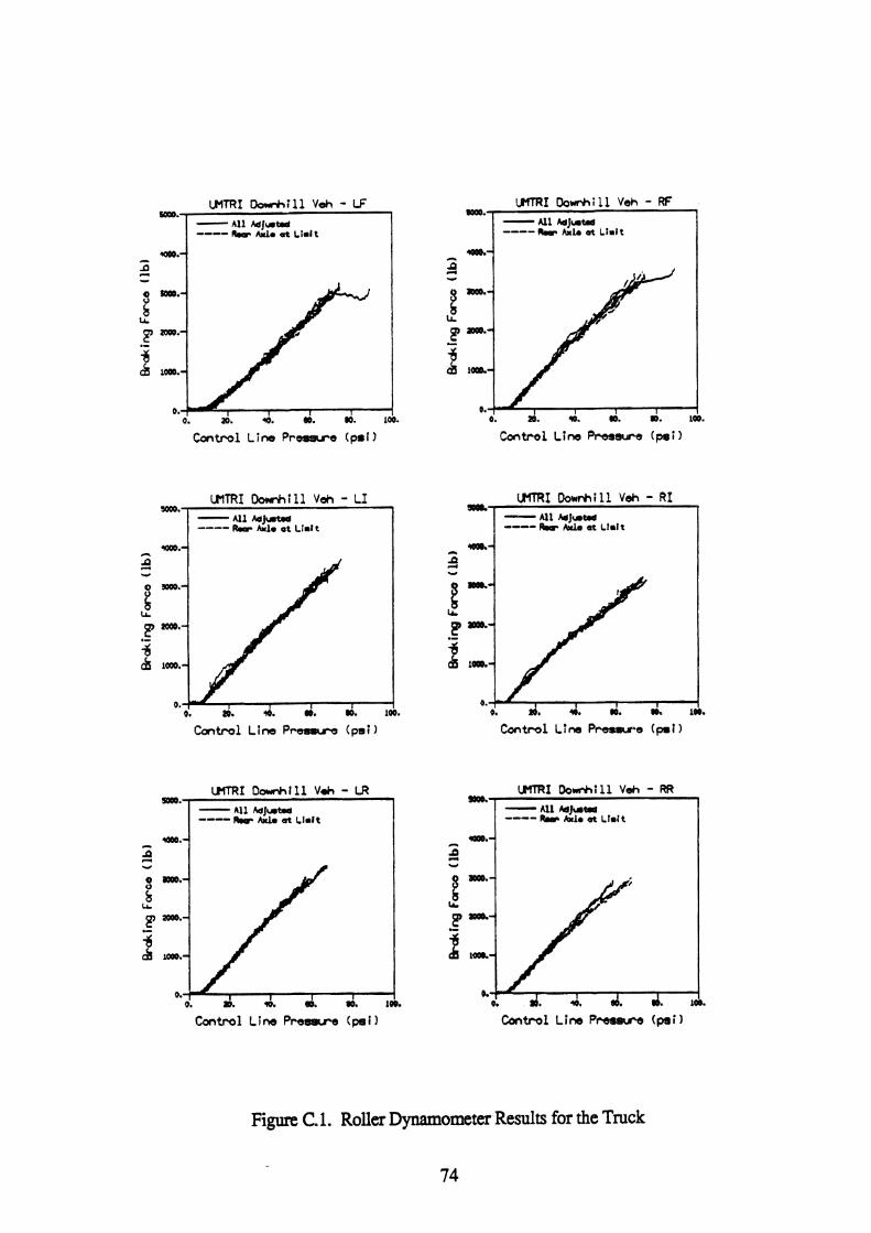
I - All M1wt.d ---- krr h l e a L i d t
5000. UlTRI M i l l Veh - LI - ---- All M j W
R.r A.1. at Lial r
h t r o l Line Pr- (psi)
sm. -1 Darnkt11 V o h - LR - ---- A l l AdJutad
w Axl. at Ll.It I
' - I o. id. i a d. IW.
Control Line P r e w e (psi)
w. CMRI Oowrhill Veh - RF - Ul ! d J ~ t d ---- b Axla at L i d t
Control Line Prosawe (pei 1
- CMTRI Dew* i ll Veh - RI - All MJwW ---- b ~ x l a cn L I U I ~
Contra1 Line Presswe (poi)
1000. LMTRI Dowrhlll vsh - RR - ---- All MJ-ta
Ru Awl* ot L1.l t
Control Line Preswra (wi)
Figure C- 1. Roller Dynamometer Results for the Truck
74

Table C.l
THRSSHOLD PRESSURES - UHTRI DOWNHILL VEHICLE Left
Auoly Release Avn Rieht
A p o l V b - a
Brakes Fully Adjusted Front
11.66 4.81 8.232 8.06 5.16 6.607 11.80 5.30 8.550 7.91 3.89 5.900 12.37 4.73 8.550 7.56 4.52 6.042
Intermediate 7.49 5.30 6.395 6.57 4.81 5.688 7.07 5.30 , 6.183 6.92 4.88 5.900 7.49 5.37 6.430 7.91 4.81 6.360
Avg
Rear
Rear Axle at Recommended Limit Front
12.86 5.65 9.257 8.69 4.31 6.501 13.07 5.09 9.080 8.48 4.45 6.466 11.52 4.73 8.126 8.69 4.03 6.360
Intermediate 8.69 5.02 6.854 7.00 4.88 5.936 7.56 5.30 6.430 6-92 4.81 5.865 8.13 5.58 6.854 7.21 5.51 6.360
Rear 8.27 6.22 7.243 6.78 5.16 5.971 7.00 5.65 6.324 7.00 4.95 5.971 7.84 5.23 6.536 7.07 4.45 5.759

Downhill - T r a c t o r L e f t F ron t
=Om**
3000.
2000.
1000. - -------. 0.
C o n t r o l Pressure ( p s i )
5000.
4000 A
4 - w
3000. a
LI 2000.
2 C 1000.
0.
C o n t r o l Pressure ( p s i )
Figure C.2. Roller Dynamometer Results for the 3-S3
76

5000. Qownhill - Tractor L e f t I n t e r
0
n d Y
3000.
E 7000.
P Lao.
0 . 0. 20. 40. W. 100.
Control Pressure (psi)
Downhill - Tractor Le f t R s c r wo. , 1
Control Pressure (psi) I
5000.
w.
20QO.
1000.
0. 0. 20. 40. LOO.
Control Pressure (psi 1
Downh f 11 - Tractor R i gh t Rear I
Control Presswe (ps i )
Figure C.2. Roller Dynamometer Results for the 3 4 3 (continued)
77

Oownhill - Trai ler Lef t Front SQ00.
Control Pressure ( p s i )
Oownhill - Trai lar L e f t Rear SOQO.
4000.
Control Prss8ure ( ps i )
Control Presswe ( ps i
wnhfll - Trallar R
h
n 4 Y
E 2ooo.
3 &
1000.
0.
Cmb-01 Presswe (psi)
Figure C.2. Roller Dynamometer Results for the 3 4 3 (continued)
78

Control Pressure ( p s i )
Hgurt C.2. Roller Dynamometer Results for the 343 (continued)
79
Trac to r R i g h t F ron t 3. :
2
2 •
. - Fuli ~ d ~ ~ ~ t i o p ---v -- ' -7-*~;i?ded~ ! f rn I it -.*....-...-
I I -.-.... +--.-----.+.-+.-d--.-" -.-- ! : I ..-.... -"++-+-..+ -.... i -.... ++-+-
---l-i-...i-4--i--...-..-i-" -+--+---4----
0. 20. 40. 60. 80. 100.
Cont ro l Pressure ( p s i )

Tractor L e f t I n termed i ate
C o n t r o l Pressure (pel
Tractor L e f t R e a r
i i i i i C-i.---..---$-..j-~----. I
". 1 4. 4. I I I 0. do. 80. 100.
C o n t r o l Pressure (psi)
Tractor Right In t e r m e d i ate 3.
, s t , ..... : ...... i ....- i ...... , I ,
, , , a , # , 1 6 , 2.*"-+ --..+...-.k.-.-I.-....i..*....)...... i......+......+.-.. -
I , I I I , I , ,
A I , I b I , I I / , I t I I I , I ..... C ..-...------ L &.............*.....a....................*..-.. .- : ! I : ! : : : :
Y , ( 0 . 0 $ 8 , 2,- .". -; ...... +...".+ ..*... ...... d'.'.. ........ 'I... " '4 ...... ;- ...... I I I 4 0 I
: I I 5 8 &++-*-- ----... ...... E ..-.-....--A-... , , # &-..-.;;..& f ie-- / .-....A # , S
, 6 I I I I ...... .... ' *ez &-..A ...-. 4 ...-. 4.- ....
V)
Control Presswe (psi)
Tractor Right Rear 1.
! . . I ! :
.... ...... .... ...... ..... 0. 1 I I
0. 20. 40. m. 4. LOO.
Control Presswe (psi )
Figure C.2. Roller Dynamometer Results for the 3 4 3 (continued)
80
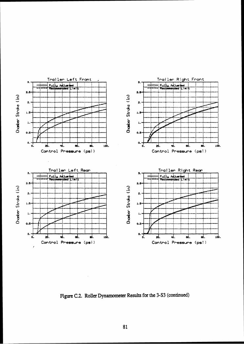
3 . . , . , . , . , r Trailer L e f t F r m t ,
I I I I I 0. 20. 40. 00- mn LOQ.
Con t r o 1 Pressure ( ps i )
3. Troller L e f t Rear
I...* - - - - < d l , m & F: !~ .M u+$. l.... i ! .-.. i : ...- L : ..... I
Control Pressure (psi ) I
T r a i l e r Right Front 3 . . . , , , , , t ~ , \
I I I I I 0. 20. 0. 00. 00. LOQ.
Control Pressure (ps i )
Trailer Right Rear 3. , I , I I.=-*.. ---7 "--ZIml* i ..... L-.L-..L : ! ! ....
" I I I I I I 0. 20. lo. 80. 80. 100.
Control Presswe (psi)
Figure C.2. R o l k Dynamometer Results for the 3 4 3 (continued)

Table C.2
TBBBSHOLD PRESSURES - DOWNHILL TEST VEUICLE
Valves Balmced, Brakes ~ d j w t e d Valves Balanced, Brake a t Linit V a h s Unbal.nmad, I r h Adjusted
& k B u n b n B B h ~ & B p b B P B O U h o B n B p B a B Y n
Trac tor Front 9.12 2.12 3.618 7.63 1.98 4.805 10.74 5.09 7.914 7.56 4.24 5.900- 16.25 4.45 10.352 14.70 3.96 9.328 9.61 2.69 6.148 7.84 2.61 5.229 9.47 3.89 6.678 7.98 4.24 6.112 15.40 4.52 9.963 14.27 4.03 9.151
10.25 3.89 7.066 6.71 2.40 4.558 9.12 4 .81 6.960 6.64 4.81 5.724 14.77 4.45 9.610 13.43 1.82 8.621
Trac to r Intermediate 13.71 2.61 8.162 12.58 2.61 7.596 14.84 3.60 9.222 12.65 3.46 8,056 17.74 8.4813.108 15.90 8.2712.083 13.36 3.32 8.338 12.22 2.54 7.384 14.06 3.25 8.656 11.94 2.90 7.420 17.10 7.84 12.472 15.62 7.07l1.341 14.13 3.46 8.798 12.51 2.83 7.667 13.92 3.67 8.798 12.37 3.18 7.773 17.95 7.21 12.578 15.69 6.7Sl1.235
Trac to r IL.u 12.44 3.18 7 .808 12.58 L. 84 7.208 13.21 4.24 8.727 12.58 2,97 7.773 17.10 7.63 12.366 15.83 6.2211.023 12 .223 .18 7.702 12.012.47 7.243 13.573.82 8.692 12 .513 .11 7.808 17.177.6312.401 15.766.6411.200 13.07 3.53 8.303 1 2 . a 2.47 7.278 12.65 3.32 7.985 12.15 3.25 7.702 16.46 7.21 11.836 15.33 6.2910.811 Avg 12.58 3.30 7.938 12.22 2.26 7.243
T r a i l e r Front 10.25 3.11 6.678 7277 3.32 5.547 9.89 4 .31 7.102 9.26 3.53 6.395
9.89 2.83 6.360 8.55 3.39 5.971 9.89 3.04 6.466 8.48 3.18 5.830 9.12 3.18 6.148 8.34 3.18 5.759 8.97 2.69 5.830 8.90 2.97 5.936
T r a i l e r Rear 8 .553 .25 5.900 8 . 4 1 1 . 9 1 5.158 11.593.67 7.632 8.693.60 6.148
1 0 . 1 8 3 . 3 2 6.748 8 .832 .05 5.44.- 9 .473 .60 6.536 8.623.60 6.112 9.47 3.25 6.360 8.55 2.19 5.370: 9.89 3.46 6.678 9.40 3.53 6.466

Table C.3 m o a t . - - T T ~ r c / w m r c Carrrdrl vchlclr (rake D l s t r i t u t im Test Prpp l~ l l
rrrtw: IJR- 7. State A in Table 1 r r a ~ ~ r :
Tractor brb
JO in5 ~nmoir r 3 11 . 3 t L
-1 (ul th d i i l a d mlnl truta at O.BiO.TV cr l lb r r t lon) ' I
YOfLS: 1) Uaa s h q rlr to wt t d to (in 100 prl I n a l l n r m o l m y p u k t q brku a t w t rrlrw M 1-t s h e I s at fl pi. 2) f u l l Conlblmttom U.. 8 dumoI r.corbr rt 56 .I/-.
lrutor QIlv: Us* 8 dlml mcordu rt 50 I/-. TrrIlu (My: u.. d I f l a d MI'S t r r r d x w rd d ia l le t rrrclout.
P
rrwtorr VQ-2 State B i n Table 1 I ra1 IU:
mts: 1) u.. *ap a i r to w( t d to g i n 100 pl I n a l l mnnlm; pktm bmkoa rr twrd: a t u t r r l r w r thm l awst cMw 11 at 9) pl. 2) f u l l C&Imtton: Uu 8 ckur*l r u m at 50 I/-.
l r u t o r Only: Uu 8 chml r.cadcr at 50 I/-. I r a i Lw mlv: rn &If lad IAllr t m r d c r r ad d l g l U l d t .
~ r t t hn: 6$ aZ -q r IOC~II~UI:

APPENDIX D
HEAT FLOW EQUATIONS
The heating of a brake is analyzed here as a simple process consisting of three parts: (1) the heat flow into the brake .due to the rate at which the brake is doing work, (2) the thermal capacity of the brake as determined by its mass (weight) and specific heat, and (3) the heat flow out of the brake (cooling) due primarily to conduction and convection.
The equations presented in this appendix pertain to this simple process. They are good
for predicting bulk temperatures of brake drums for slowly changing temperatures such as those that occur during mountain descents. More complicated equations are needed to predict the distribution of brake temperatures across the drum and in the linings as may be of interest in rapid stops. Also, if the brakes become very hot, cooling due to radiation
may be important enough to require special terms in the cooling characteristics. Experience, using the equations presented here, has shown that they will provide
reasonable predications of brake temperatures if thexalues of the cooling coefficients are determined experimentally.
The equation describing heat flow is as follows:
P = m Cp (dT1dt) - hv (T - Ta)
where
P = the energy rate, i.e., the rate of doing work, i.e., the power or heat flow into
the brake (ft-lblsec)
m = weight (lb) (100 lb for example)
Cp = specific heat (approximately 100 ft-lbAb % for cast iron drums)
dT/dt = the time rate of change of the bulk temperature (average temperature of the brake)
hv = cooling rate which is usually treated as a linear function of velocity starting
from a rate corresponding to the cooling at zero velocity (ft-lbfi sec)

T = bulk temperature eF)
Ta = ambient temperature (v Given values for m, Cp, Ta, and h, differential equation (Dl) can be solved for
temperature as a function of time if P is available as a function of time. The simplified
model, used for making the predictions used in Appendix A, performs this type of
calculation for each brake. The power to each brake is determined by the proportioning of
braking effort throughout the brake system plus the work rate required to maintain or
reduce speed on various sections of the vehicle's route.
In connection with Table 6, equation (Dl) has been "integrated" to obtain the following
expression which can be solved for the cooling rate (h) at a particular speed (see Table 6 for
the resulting equation). For approximately constant velocity,
Energy = m Cp (Thf - THi) - hv Ft(TH) + THA (tf - ti)] 0 2 )
where
THf = Final temperature, ?F
THi = Initial temperature, ?F
THa = Ambient temperature, 9
tf = Final time (braking ends), sec
ti = Initial time (braking starts), sec
Energy = Total work done by the brake, ft lb
Int(TH) = Integral of brake temperature from ti to tf, ?F sec
hv = cooling rate, ft 1bfF sec
To experimentally determine h, the energy into the brake (i.e., the work done by the brake) is evaluated (perhaps by integrating the product of brake torque multiplied by wheel
speed). The bulk temperature of the brake, as represented by the readings of the thermocouples installed on the outside of the drum, is measured and recorded. Then the integral of the bulk tempera& is computed from ti to tf. Once these steps are completed,
equation (D2) can be solved for the value of hv at the speed used in the experiment.
