the infamous upper tail

The Infamous Upper Tail

Svante Janson,1 Andrzej Rucinski2,*1Uppsala University, Uppsala, Sweden2A. Mickiewicz University, Poznan, Poland

Received 27 December 2000; accepted 26 September 2001Published online xx Month 2002 in Wiley InterScience (www.interscience.wiley.com).DOI 10.1002/rsa.10031

ABSTRACT: Let � be a finite index set and k � 1 a given integer. Let further � � [�]�k be anarbitrary family of k element subsets of �. Consider a (binomial) random subset �p of �, where p� ( pi : i � �) and a random variable X counting the elements of � that are contained in thisrandom subset. In this paper we survey techniques of obtaining upper bounds on the upper tailprobabilities �(X � � � t) for t � 0. Seven techniques, ranging from Azuma’s inequality to thepurely combinatorial deletion method, are described, illustrated, and compared against each otherfor a couple of typical applications. As one application, we obtain essentially optimal bounds for theupper tails for the numbers of subgraphs isomorphic to K4 or C4 in a random graph G(n, p), forcertain ranges of p. © 2002 Wiley Periodicals, Inc. Random Struct. Alg., 20: 317–342, 2002

1. INTRODUCTION

Let � be a finite index set and k � 1 a given number, and let [�]�k be the family of allsubsets A � � with �A� � k. Suppose that IA, A � [�]�k, is a family of nonnegativerandom variables such that each IA is independent of {IB : B � A � �}. Let X :� ¥A

IA and � :� �X � ¥A �IA.In this paper we survey techniques of obtaining upper bounds on the upper tail

probabilities �(X � � � t) for t � 0. In many instances such inequalities come togetherwith their lower tail counterparts as a two-sided concentration result. This is the case ofcelebrated Azuma’s and Talagrand’s inequalities (see the next section). The simplestsituation takes place when k � 1. Then X is a sum of independent summands, and if these

Correspondence to: Svante Janson; e-mail: [email protected].*Supported by KBN grant 2 P03A 032 16.© 2002 Wiley Periodicals, Inc.

317

happen to be 0–1 random variables, Chernoff’s bounds apply. With �( x) � (1 �x)log(1 � x) � x, x � �1 [and �( x) � � for x � �1], we have (see e.g., [1, 7, 9,Theorem 2.8])

��X � � � t � exp�� t

�� exp��t2

2�� t/3�, t � 0, (1)

��X � � � t � exp��t

� �� exp��t2

2��, t � 0. (2)

There is a little asymmetry between the lower and upper tail, but for t � � the order ofmagnitude of the exponents is the same.

For arbitrary k, a special case of our general framework can be described as follows.Suppose that �i, i � �, is a family of independent 0–1 random variables and that IA �i�A �i when A � � for a given family � � [�]�k, while IA � 0 when A � �. In otherwords, the indicator random variables �i describe a (binomial) random subset �p of �,where p � ( pi : i � �), pi � �(�i � 1) [we write �p if pi � p for all i], and X is thenumber of elements of � that are contained in this random subset. For the lower tail of thedistribution of X, the following analogue of the Chernoff bound holds ([8, 9, Theorem2.14]).

Theorem 0. Let X � ¥A�� IA as above, and let � � �X � ¥A �IA and �� ¥¥A�B��(IAIB). Then, with �( x) � (1 � x)log(1 � x) � x, for 0 � t � �,

��X � � � t � exp��t/��2

�� exp��t2

2�� .

It follows from the FKG inequality (see, e.g., [9]) that the above bound is tight: If t ��, �� o(�) and max pi � o(1), then

��X � 0 � exp ��1 � o�1�.

However, an upper tail analogue cannot be true in general. One slightly artificialcounterexample is presented in [9, Remark 2.17]. A more natural one is the followingfrom [20] (here slightly adapted).

(Counter) Example. Let � � [n]2, k � 3, and � be the family of the edge sets of alltriangles in Kn, the complete graph on [n]. Furthermore, let pi � p � p(n) for all i �[n]2. Then X is simply the number of triangles in the random graph G(n, p). Assuming

nlog n �� p � o(1), fix three disjoint subsets of vertices, each of order v � (2�)1/3, whererecall � � �X. Then with probability p3v2

there is a complete tripartite subgraph on thethree sets, yielding v3 � 2� triangles in G(n, p), and thus

�log ��X � 2� � 3v2log1

p� 3�2�2/3log n ��

318 JANSON AND RUCINSKI

so �(X � 2�) �� e�c� for every c � 0.

In the next section we present several techniques of obtaining exponential bounds onthe upper tail of X. Then, in the last section we illustrate them by a few examples andbased on these examples, we compare them against each other. For X being the numberof copies of K4 in a random graph G(n, p), one of our methods yields in a range of p anoptimal bound, which means a bound that up to a logarithmic factor in the exponentmatches the lower bound obtained by Vu’s (counter)example. For the number of copiesof C4, two of the methods yield an optimal bound for certain ranges of p.

We use ck to denote various positive constants depending on k only.This paper is meant to be an extension of Section 2.6 of [9]. We hope that the examples

treated here can serve as inspiration and suggestions for future applications of themethods.

2. METHODS

2.1. Inequalities Based on Lipschitz Condition

The first method is a version of Azuma’s inequality [7] tailored for combinatorialapplications (see e.g. [12], [13], and [9, Remark 2.28]).

Theorem 1. Let Z1, . . . , ZM be independent random variables, with Zj taking values ina set �j. Assume that a function f : �1 � �2 � . . . � �M 3 � satisfies, for someconstants bj, j � 1, . . . , M, the following Lipschitz condition:

(L) If two vectors z, z� � �1 � �2 � . . . ��M differ only in the jth coordinate, then� f(z) � f(z�)� � bj.

Then, the random variable X � f(Z1, . . . , ZM) satisfies, for any t � 0,

��X � � � t � exp��2t2��1

M

bj2�, (3)

��X � � � t � exp��2t2��1

M

bj2�. (4)

Returning to the random set �p, one typically defines the random variables Zj via therandom indicators �i, i � �. Given a partition A1, . . . , AM of �, each Zj is then takenas the random vector (�i : i � Aj) � {0, 1}Aj, and for a given function f : 2� 3 �, theLipschitz condition (L) in Theorem 1 is equivalent to saying that for any two subsets A,B � �, � f( A) � f(B)� � bj whenever the symmetric difference of the sets A and B iscontained in Aj.

When � � [n]2 and so �p � G(n, p), there are two common choices of the partition[n]2 � A1 � . . . � AM. The vertex exposure martingale corresponds to the choice M �n and Aj � [ j]2[ j � 1]2. The edge exposure martingale is one in which M�(2

n) and �Aj�

THE INFAMOUS UPPER TAIL 319

� 1 for each j. For example, with bj � 1, edge exposure is applicable provided therandom variable X changes by at most 1 if a single edge is added or deleted, while vertexexposure is applicable provided X changes by at most 1 if any number of edges incidentto a single vertex are added and/or deleted.

Talagrand [17] found another method that yields similar results. A combinatorialversion of the Talagrand inequality requires, besides the Lipschitz condition, one more,quite technical condition, but in return it yields very often stronger bounds than Azuma’sinequality. (For proof, see, e.g., [17] or [9, Theorem 2.29].)

Theorem 2 (Talagrand). Let Z1, . . . , ZM be independent random variables, with Zj

taking values in a set �j. Assume that a function f : �1 � �2 � . . . � �M3 � satisfies,for some constants bj, j � 1, . . . , M, and some function , the following two conditions:

(L) If two vectors z, z� � �1, . . . , �M differ only in the jth coordinate, then � f(z) �f(z�)� � bj.

(C) If z � � and r � � with f(z) � r, then there exists a set J � {1, . . . , M} with¥j�J bj

2 � (r), such that for all y � � with yj � zj when j � J, we have f(y) �r.

Then, the random variable X � f(Z1, . . . , ZM) satisfies, for any r � � and t � 0,

��X � r � t��X � r � e�t2/4�r. (5)

In particular, if m is a median of X, then for every t � 0,

��X � m � t � 2e�t2/4�m (6)

and

��X � m � t � 2e�t2/4�m�t. (7)

Remark 1. A recent inequality of Boucheron, Lugosi, and Massart [2] is sometimes aninteresting alternative to Talagrand’s inequality; in several applications it yields essen-tially the same result (with better constants). We do not, however, see any way to use theirinequality in the set-up treated here.

2.2. Kim–Vu Concentration via Average Smoothness

Inequalities from the previous section become weaker when the Lipschitz coefficient arelarge. Kim and Vu in [11] developed a method yielding concentration bounds whichdepend only on the “average” Lipschitz coefficients, typically much smaller than the“worst-case” ones. Very recently Vu wrote an excellent expository paper on that method[21].

Their setup is less general than that of Azuma’s and Talagrand [though, still moregeneral than that of Theorem 0]. Let X � X(�i : i � � � [N]) be a polynomial of degreek, where again �i are independent random 0–1 variables. For a nonempty set A � �[k] let


�AX be the partial derivative of X with respect to the variables in A and define, for j �0, . . . , k, �j(X) � max�A��j �(�AX). (Thus �0(X) � �(X) � �.)

We begin with the Main Theorem of [11], the first main theorem proved by thismethod.

Theorem 3A (Kim and Vu). For any � � 1, if � � �1(X), then

��X � �� ck�k��1�X � exp �� k � 1log N�. (8)

The above theorem is derived from a more general, but more technical, concentrationresult, also proved in [11]. Let, for each i � 1, . . . , M,

Ei � ��X��1, . . . , �i�1, �i � 1 � ��X��1, . . . , �i�1, �i � 0�.

[Note that, as a conditional expectation, Ei is a random variable which is a function of(�1, . . . , �i�1).] Let further M � maxi Ei, W � ¥i piEi and V � ¥i piqiEi

2.

Theorem 3B (Kim and Vu). Let a, v, � be positive numbers such that 0 � � � v/a2.Then

��X � �� v 2 exp ��/4� � ��M � a or V � v � 2 exp ��/4�

� �i

��Ei � a � ��W � v/a. (9)

These results have been developed further and successfully applied to a variety ofproblems by Kim and Vu (see, e.g., [11, 18, 19, 20], and the survey [21], where alsofurther references are given). In particular, Vu [21, Corollary 3.4] has proved thefollowing general and widely applicable result, using Theorem 3B and induction. Forfurther similar results see [18, 21]. It is easily seen that Theorem 3C always yields at leastas strong bounds as Theorem 3A; this is illustrated by the examples in Section 3.

Theorem 3C (Vu). Let �0 � �1 � . . . � �k and � be positive numbers such that �j ��j(X), 0 � j � k, and �j/�j�1 � � � j log n, 0 � j � k � 1. Then

��X � �� 0�1 � Ckexp �ck��. (10)

2.3. Combinatorial Techniques

In this subsection we collect techniques that require only an elementary, combinatorialargument. We will be assuming throughout that all elements of � have the same size k,and that for all i, pi � p for some 0 � p � 1. Thus � � �X � ��pk. For convenience,the deviation parameter t will be expressed here in the form t � ��X � ��, though �,in general, is not necessarily a constant, and we will for simplicity only consider the case0 � � � 1. Finally, set �� N.


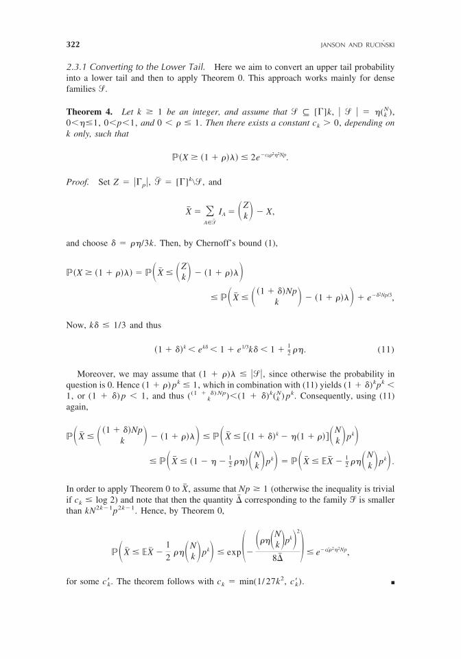
2.3.1 Converting to the Lower Tail. Here we aim to convert an upper tail probabilityinto a lower tail and then to apply Theorem 0. This approach works mainly for densefamilies �.

Theorem 4. Let k � 1 be an integer, and assume that � � [�]k, � � � � �(kN),

0��1, 0�p�1, and 0 � � � 1. Then there exists a constant ck � 0, depending onk only, such that

��X � �1 � �� 2e�ck�2�2Np.

Proof. Set Z � ��p�, �� [�]k�, and

X� � �A��

IA � �Zk� � X,

and choose � � ��/3k. Then, by Chernoff’s bound (1),

��X � �1 � �� X� � �Zk� � �1 � ��

� ��X� � � �1 � �Npk � � �1 � �� e��2Np/3,

Now, k� � 1/3 and thus

�1 � �k ek� 1 � e1/3k� 1 �12 ��. (11)

Moreover, we may assume that (1 � �)� � ��, since otherwise the probability inquestion is 0. Hence (1 � �) pk � 1, which in combination with (11) yields (1 � �)kpk �1, or (1 � �) p � 1, and thus ( k

(1 � �) Np)�(1 � �)k(kN) pk. Consequently, using (11)

again,

��X� � � �1 � �Npk � � �1 � �� X� � ��1 � �k � ��1 � ��N

k �pk�� X� � �1 � � �

12 ��N

k �pk� � ��X� � �X� �12 ��N

k �pk� .

In order to apply Theorem 0 to X� , assume that Np � 1 (otherwise the inequality is trivialif ck � log 2) and note that then the quantity �� corresponding to the family �� is smallerthan kN2k�1p2k�1. Hence, by Theorem 0,

��X� � �X� �1

2��N

k �pk� � exp��N

k�pk�2

8�� e�c�k�2�2Np,

for some c�k. The theorem follows with ck � min(1/ 27k2, c�k). �


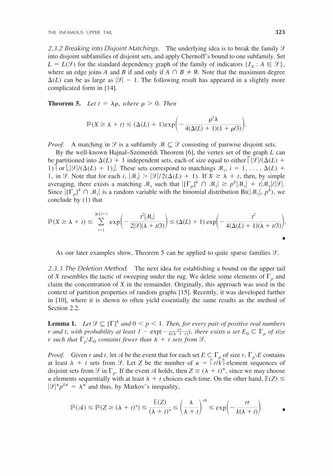
2.3.2 Breaking into Disjoint Matchings. The underlying idea is to break the family �into disjoint subfamilies of disjoint sets, and apply Chernoff’s bound to one subfamily. SetL � L(�) for the standard dependency graph of the family of indicators {IA : A � �},where an edge joins A and B if and only if A � B � �. Note that the maximum degree�(L) can be as large as �� 1. The following result has appeared in a slightly morecomplicated form in [14].

Theorem 5. Let t � ��, where � � 0. Then

��X � � � t � ��L � 1exp��2�

4��L � 1�1 � �/3�.

Proof. A matching in � is a subfamily � � � consisting of pairwise disjoint sets.By the well-known Hajnal–Szemeredi Theorem [6], the vertex set of the graph L can

be partitioned into �(L) � 1 independent sets, each of size equal to either ��/(�(L) �1) or ��/(�(L) � 1). These sets correspond to matchings �i, i � 1, . . . , �(L) �1, in �. Note that for each i, ��i� � ��/ 2(�(L) � 1). If X � � � t, then, by simpleaveraging, there exists a matching �i such that �[�p]k � �i� � pk��i� � t��i�/��.Since �[�p]k � �i� is a random variable with the binomial distribution Bi(��i�, pk), weconclude by (1) that

��X � � � t � �i�1

��L�1

exp��t2��i�

2�� t/3� � ��L � 1 exp��t2

4��L � 1�� t/3�.

�

As our later examples show, Theorem 5 can be applied to quite sparse families �.

2.3.3 The Deletion Method. The next idea for establishing a bound on the upper tailof X resembles the tactic of sweeping under the rug. We delete some elements of �p andclaim the concentration of X in the remainder. Originally, this approach was used in thecontext of partition properties of random graphs [15]. Recently, it was developed furtherin [10], where it is shown to often yield essentially the same results as the method ofSection 2.2.

Lemma 1. Let � � [�]k and 0 � p � 1. Then, for every pair of positive real numbersr and t, with probability at least 1 � exp(� k(� � t)

rt ), there exists a set E0 � �p of sizer such that �pE0 contains fewer than � � t sets from �.

Proof. Given r and t, let � be the event that for each set E � �p of size r, �pE containsat least � � t sets from �. Let Z be the number of � � r/k-element sequences ofdisjoint sets from � in �p. If the event � holds, then Z � (� � t)�, since we may choose� elements sequentially with at least � � t choices each time. On the other hand, �(Z) ��pk� � �� and thus, by Markov’s inequality,

�� Z � �� t� ��Z

�� t� � � �

� � t�r/k

� exp��rt

k�� t�. �


In subsection 3.3 we show a direct application of Lemma 1. Now we derive from it agenuine bound on the upper tail of X in terms of the maximum degree in the subhyper-graph �p � � � [�p]k. Let, for I � �, YI :� ¥J�I XJ and

Y*1 :�maxi��

Y i�.

Clearly, Y*1 � �(�p) and there are at most rY*1 elements of �p which could have beendestroyed by removing r elements from �p.

Theorem 6A. Let t � ��, 0 � � � 1. Then, for every real r � 0,

��X � � � t � exp ��r/3k� � ��Y*1 � t/2r.

Proof. If X � � � t and Y*1 � t/ 2r, then for every set E � �p with �E� � r, �pEcontains at least

X � rY*1 � � � t/2

sets from �. By Lemma 1 the probability of the latter event is at most

exp��rt/2

k�� t/2� � exp��r

3k �. �

The probability �(Y*1 � t/ 2r) can be annihilated by choosing r � t/ 2�(�). Thisgives as a corollary a bound in terms of maximum degree in �.

Theorem 6B. Let t � ��, 0 � � � 1. Then

��X � � � t � exp ��2�/�6k��.

Since �(�) � 1 � �(L(�)) � k�(�), this theorem yields almost the same boundas Theorem 5.

Alternatively, one can bound �(Y*1 � t/ 2r) � ¥ �(Y{i} � t/ 2r) in Theorem 6A andhope for the best. For k � 2, Y{i} is the number of surviving neighbors of vertex i, whichis a sum of independent random variables, so Chernoff’s inequality can be applied. Fork � 2 each Y{i} is a sum of dependent random variables but of the same type as X, whichgives room for induction. One way of doing it leads to the following result, the proof ofwhich is presented in [10] (cf. Corollary 4.1 there). Let �j � �j(�) be the maximumnumber of elements of � containing a given j-element set, j � 0, . . . , k.

Theorem 6C. Let �*j � �jpk�j [thus �*0 � �]. Then, with ck � 1/12k, and for all 0 �

� � 1,

��X � �1 � �� 2Nk�1exp��ck min1�j�k

��2�

�*j �1/j�.


2.3.4 Approximating by a Disjoint Subfamily. Our last method originates in Spencer[16] (cf. Example 1, below). Let X0 be the largest number of disjoint sets of � which arepresent in �p. Clearly, X � X0, but sometimes X is not much larger than X0. Intuitively,X0 should have a distribution similar to that of a sum of independent random variables,and thus a Chernoff-type bound could be true. Our next lemma makes it precise.

Lemma 2. If t � 0, then, with �( x) � (1 � x)log(1 � x) � x and � � �X,

��X0 � � � t � exp�� t

�� exp��t2

2�� t/3�. �

For the proof of Lemma 2, which is similar to the proof of Lemma 1, see [9, Lemma2.46].

In order to relate X to X0 we invoke a simple graph theoretic fact. For an arbitrary graphG set �(G) for its independence number, �(G) for the size of the largest inducedmatching in G, and �e(G) for the maximum of �NG(v) � NG(v�)� over all pairs (v, v�)of adjacent vertices of G. Note that �e(G) � 2�(G).

Lemma 3. For every graph G, we have �V(G)� � �(G) � �(G)�e(G).

Proof. Let M be the set of edges in a maximal induced matching of G. The verticesoutside M can be divided into two groups: those adjacent to M [at most �(G)(�e(G) �2) of them] and those which are not. The latter group of vertices form an independent setin G, and the lemma follows. �

Consider the intersection graph Lp � L(�p) of �p � � � [�p]k, in which everyvertex represents one set of �p, and the edges join pairs of vertices representing pairs ofintersecting sets. (Note that Lp is an induced subgraph of L defined above.) Then X is thenumber of vertices and X0 is the independence number of Lp. Thus Lemma 3 implies that

X � X0 � ��Lp�e�Lp � X0 � 2��Lp��Lp. (12)

We have already estimated the probability that X0 is large; hence estimates of �(Lp)and �(Lp) yield bounds on the upper tail of X. This leads to the following result. Recallthat �j � �j(�) is the maximum number of elements of � containing a given j-elementset, j � 0, . . . , k.

Theorem 7. Define R�� max1�j�k�1(jk)��jp

k�j, where ��j � �j � 1. Then, for everyt � 0 and r � R,

��X � � � t � exp��t2

8� � 2t� � �k � 1exp �r� � ��Y*1 �t

12k�k � 1r�. (13)

Remark 2. Very often the third term can be bounded (e.g., by a Chernoff inequality, seethe examples in Section 3) by exp(��(t/r)). Then, if, in addition, t � �(�) 3 �, thefirst term is smaller than the sum of the other two (either r or t/r is not greater than �t),


and therefore can be ignored. Also, note that for fixed �, if we ignore the first term, we areup to constants in the exponents left with the same bound as Theorem 6A, although nowonly for r � R. Hence the above bound then is never better (up to constants in theexponent) than that from Theorem 6A, and it yields essentially the same result when theoptimal r for Theorem 6A satisfies r � R.

Proof. By (12), for any � � 0,

��X � � � t � ��X0 � � � t/2 � ��Lp � � � ��Lp � t/�4�.

By Lemma 2, the first term is smaller than exp(�2(� � t/6)t2/4 ) � exp(�8��2t

t2

). For thethird term observe that �(Lp) � k�(�p) � kY*1, so �(�(Lp) � t/4�) � �(Y*1 �t/(4k�)).

It remains to estimate �(�(Lp) � �). First note that an induced matching in Lp withm edges corresponds to 2m distinct sets Ai, Bi � �p, 1 � i � m, such that Ai � Bi ��, but Ai � Aj � Ai � Bj � Bi � Bj � �, i � j. Consequently, if � � {A � B : A,B � �, A � B, A � B � �}, then �(Lp) is the maximum size of a disjoint subfamilyof �p, i.e., �(Lp) � �(L(�p)). Thus, �(Lp) is a random variable of the same type as X0,except that � is not a uniform hypergraph. To overcome this mild difficulty, we write �� j�1

k�1 �j, where �j � {A � B : A, B � �, �A � B� � j}, and thus have, with Y0j

� �(L(�pj )),

��Lp � ��L� �j�1

k�1

�pj��

j�1

k�1

Y0j .

Hence,

��Lp � � � �j�1

k�1

��Y0j � �/�k � 1.

In order to apply Lemma 2 to Y0j , we need to estimate the expected size of �p

j . For eachA � � there are at most (j

k)��j choices of B � � with �A � B� � j. Hence, setting Yj ��p

j �,

�Yj � � kj ��j��p2k�j � � k

j ��jpk�j� � R � r,

and, by Lemma 2, with � � 3(k � 1)r,

��Y0j � �/�k � 1 � ��Y0

j � 3r � ��Y0j � �Yj � 2r � e�r. �

Sometimes, �(Lp) and �(Lp) [or �e(Lp)] can be estimated with more ease. This is thecase of the next example from [16] where this technique originated.


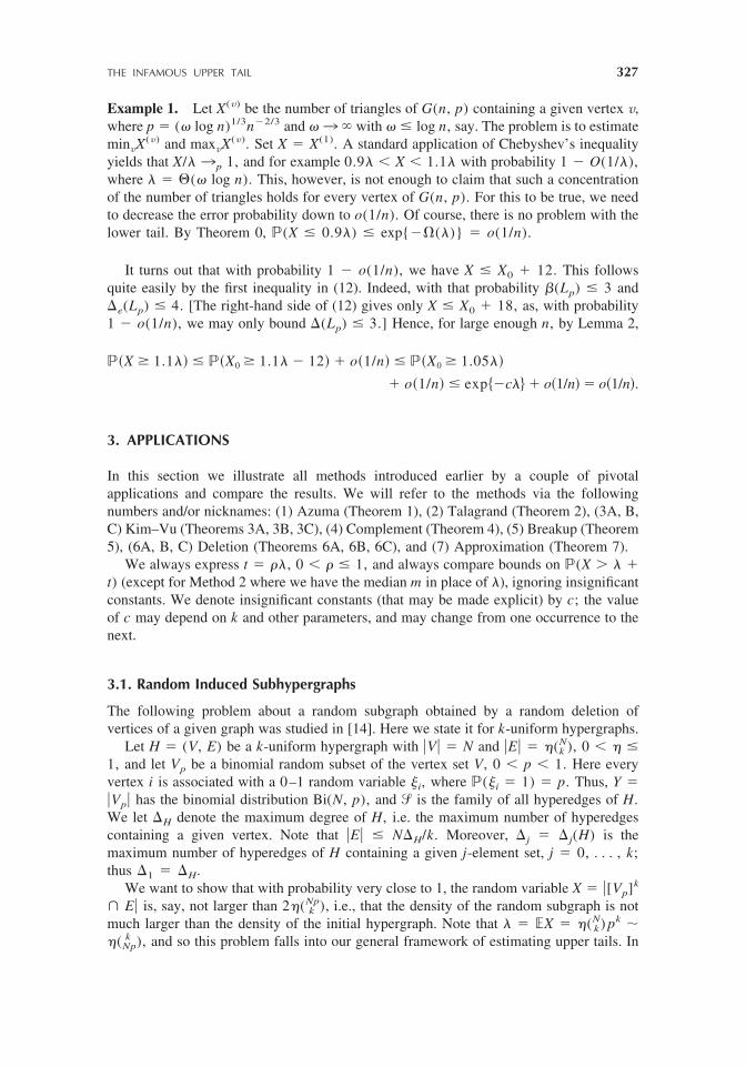
Example 1. Let X(v) be the number of triangles of G(n, p) containing a given vertex v,where p � (� log n)1/3n�2/3 and �3 � with � � log n, say. The problem is to estimateminvX(v) and maxvX(v). Set X � X(1). A standard application of Chebyshev’s inequalityyields that X/� 3p 1, and for example 0.9� � X � 1.1� with probability 1 � O(1/�),where � � �(� log n). This, however, is not enough to claim that such a concentrationof the number of triangles holds for every vertex of G(n, p). For this to be true, we needto decrease the error probability down to o(1/n). Of course, there is no problem with thelower tail. By Theorem 0, �(X � 0.9�) � exp{��(�)} � o(1/n).

It turns out that with probability 1 � o(1/n), we have X � X0 � 12. This followsquite easily by the first inequality in (12). Indeed, with that probability �(Lp) � 3 and�e(Lp) � 4. [The right-hand side of (12) gives only X � X0 � 18, as, with probability1 � o(1/n), we may only bound �(Lp) � 3.] Hence, for large enough n, by Lemma 2,

��X � 1.1� � ��X0 � 1.1� � 12 � o�1/n � ��X0 � 1.05�

� o�1/n � exp �c�� o�1/n � o�1/n.

3. APPLICATIONS

In this section we illustrate all methods introduced earlier by a couple of pivotalapplications and compare the results. We will refer to the methods via the followingnumbers and/or nicknames: (1) Azuma (Theorem 1), (2) Talagrand (Theorem 2), (3A, B,C) Kim–Vu (Theorems 3A, 3B, 3C), (4) Complement (Theorem 4), (5) Breakup (Theorem5), (6A, B, C) Deletion (Theorems 6A, 6B, 6C), and (7) Approximation (Theorem 7).

We always express t � ��, 0 � � � 1, and always compare bounds on �(X � � �t) (except for Method 2 where we have the median m in place of �), ignoring insignificantconstants. We denote insignificant constants (that may be made explicit) by c; the valueof c may depend on k and other parameters, and may change from one occurrence to thenext.

3.1. Random Induced Subhypergraphs

The following problem about a random subgraph obtained by a random deletion ofvertices of a given graph was studied in [14]. Here we state it for k-uniform hypergraphs.

Let H � (V, E) be a k-uniform hypergraph with �V� � N and �E� � �(kN), 0 � � �

1, and let Vp be a binomial random subset of the vertex set V, 0 � p � 1. Here everyvertex i is associated with a 0–1 random variable �i, where �(�i � 1) � p. Thus, Y ��Vp� has the binomial distribution Bi(N, p), and � is the family of all hyperedges of H.We let �H denote the maximum degree of H, i.e. the maximum number of hyperedgescontaining a given vertex. Note that �E� � N�H/k. Moreover, �j � �j(H) is themaximum number of hyperedges of H containing a given j-element set, j � 0, . . . , k;thus �1 � �H.

We want to show that with probability very close to 1, the random variable X � �[Vp]k

� E� is, say, not larger than 2�( kNp), i.e., that the density of the random subgraph is not

much larger than the density of the initial hypergraph. Note that � � �X � �( kN) pk �

�(Npk ), and so this problem falls into our general framework of estimating upper tails. In


fact, this is precisely the setup of our combinatorial methods 4–7 described in generalterms in Section 2. Below, we study asymptotics as N 3 �, where �, p, and � maydepend on N, with � � 1, while k � 2 is fixed. Throughout we assume that Np 3 �, andin particular Np � 1.

We will try all seven methods in two basic cases. In the general case, where noassumption is made on H, we will use the trivial bounds �j(H) � Nk�j, j � 1, . . . , k.In the highly regular case (and presumably sparse, meaning �3 0) we will be assumingthat �j � �(�Nk�j), j � 1, . . . , k � 1. (The unspecified constants c below may dependon the constants implicit in this �.) Note that �0 � �E� � �(�Nk) by definition, while�k � 1 unless H is empty.

As a warm-up consider first the special case in which H is the complete k-uniformhypergraph KN

k , i.e., � � 1. Then X � (kY) � Yk/k!, and � � (Np)k(1/k! � o(1/Np)).

Hence, assuming �Np is large enough,

��X � �1 � �� Yk � �1 � �/2�Npk

� ��Y � �1 � �/21/kNp � ��Y � �1 ��

3k�Np� ,

and by Chernoff’s bound (1), we obtain

��X � �1 � �� exp �cp2Np�. (14)

This bound is essentially sharp and we will use it to measure the accuracy of all ourmethods applied to the general case.

1. Azuma. Adding/deleting a vertex may change the value of X by at most the degreeof that vertex. Thus, applying Theorem 1 with bi � degH(i) we obtain the bound

exp��c�2�2N2k�1p2k

�H2 �.

2. Talagrand. Here again the Lipschitz condition is satisfied with bi � degH(i).However, the obvious choice (r) � N�H

2 yields only the same bound as Azuma,with an inferior constant. To get a better estimate, we have to modify X by a sortof truncation. Let

X� � max ��V��k � E� : V� � Vp, �V�� 2Np�.

Clearly, X� satisfies condition (L) with the same constants bi as X does, andcondition (C) with (r) � 2Np�H

2 . By Chernoff’s bound (1),

��X � X� � ��Vp� � 2Np � e�cNp.

This and (7) yield the bound

exp��c�2�2N2k�1p2k�1

�H2 � � e�cNp 2 exp��c

�2�2N2k�1p2k�1

�H2 � .


3A. Kim–Vu A. We can write

X � �A��

i�A

�i.

Thus,

�AX � �A�B��

i�BA

�i,

and,

�1�X � max1�j�k

�j�H pk�j � max1�j�k

�Npk�j � �Npk�1. (15)

Hence, (8) with l � ck�1/k�1/k�1/2k(�1(X))�1/2k implies (the case �1(X) � � is

trivial here, since then � is bounded)

��X � �� Nk�1exp �cp1/k��Np1/ 2k�. (16)

In the highly regular case, �1(X) � �(max[1, �(Np)k�1]) and the exponent in(16) is improved to �c�1/k(Np)1/2k if �(Np)k�1 � 1 and �cp1/k�1/2k(Np)1/2

otherwise.3B. Kim–Vu B. Observe that

Ei � �j�0

k�1 �i�A�E,�A�i��j

pj l�A��i�1�

�l.

This is a polynomial of degree k � 1, so in principle one could apply inductionhere. However, as this approach seems to be quite complicated, we referinstead to Theorem 3C (see below), where the work with the induction alreadyhas been done, in a general setting, by Vu [21].

We here thus focus on the case k � 2, i.e., the case of graphs, because onlythen Ei becomes a sum of independent variables ( j � 0) and a constant term( j � 1). Indeed, for k � 2,

Ei � �j�i

i, j��E

�j � �j�i

i, j��E

p � Z � p�H,

where Z � Bi(�H, p). Also,

W � p �i

Ei � p�HY � p2�E�.

By Chernoff’s bound (1), �(Y � 3Np) � e�Np, and so, with probability at least1 � e�Np, we have W � 4�HNp2. Now, choose a � bp�H, where b � 9, and v� 4a�HNp2. By (1), with �Z � �Hp,

��Ei � a � ��Z � �b � 1�Z � ��Z � �Z � �b � 2�Z

� exp��b � 2�Z,


where �(b � 2) � (b � 1)log(b � 1) � b � 2 � b, because log(b � 1) � 2.Hence, by Theorem 3B, setting � � �2�2/v and checking that � � v/a2 (thisfollows from � � N�Hp2), we obtain the estimate

��X � �1 � �� 2e��/4 � Ne�bp�H � e�Np. (17)

We have to choose b optimally. We would like �/4 � bp�H, i.e. b � 18 ��(N �

1)N1/2�H�3/2, but also b � 9. Thus, choosing b � max(1

8 ��(N/�H)3/2, 9) in (17)we find, since then �/4 � v/(4a2) � Np/b � Np,

��X � �1 � �� N � 3e��/4

� 2N exp��c��N3/ 2p

�H1/ 2 � if ��N/�H3/ 2 � 72,

2N exp��c�2�2N3p

�H2 � otherwise.

3C. (Kim–)Vu C. We have, generalizing (15),

�j�X � maxi�j

�i�Xpk�i.

We thus need to find � and �0, . . . , �k such that ��0�1 � ��, �j ��j(H) pk�j, 0 � j � k, and �j/�j�1 � � � j log N, 0 � j � k � 1.

It is easily checked that if Np � 2k log N, then these conditions are satisfiedwith �0 � � � �(�(Np)k), �j � (Np)k�j, 1 � j � k, and � � �2�2/�0�1 ��2�/�1 � �(�2�Np). (It is also easily checked that these choices are essentiallyoptimal without further assumptions.) Hence,

��X � �1 � �� C exp��c� � C exp��c�2�Np, Np � 2k log N.

As a trivial consequence, for any N and p,

��X � �1 � �� N exp��c�2�Np.

In the highly regular case, we instead choose �j � C max((2�)k�j, �(Np)k�j),0 � j � k, and � � c min(�2/k�1/kNp, �2Np); it is easily checked that theconditions then are satisfied, provided C is large, c is small, and � � k log N.Consequently, in the highly regular case,

��X � �1 � �� N exp��c min��2/k�1/kNp, �2Np.

4. Complement. By Theorem 4,

��X � �1 � �� 2e�c�2�2Np.

5. Breakup. By Theorem 5, with �(L) � k�H,

��X � �1 � �� k�Hexp��2�

4k�H�1 � �/3�.

6A. Deletion A. As for Theorem 3B, we consider only the case k � 2; for larger k onecan use induction, but we refer instead to Theorem 6C, where the induction


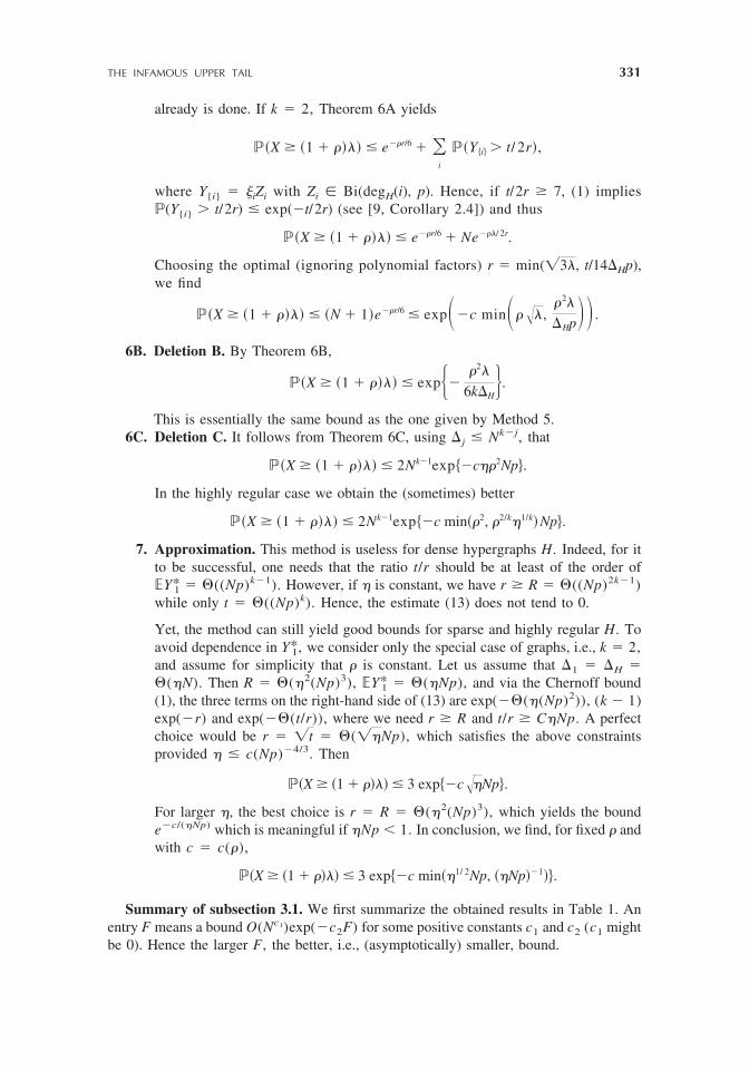
already is done. If k � 2, Theorem 6A yields

��X � �1 � �� e��r/6 � �i

��Y i� � t/ 2r,

where Y{i} � �iZi with Zi � Bi(degH(i), p). Hence, if t/2r � 7, (1) implies�(Y{i} � t/2r) � exp(�t/2r) (see [9, Corollary 2.4]) and thus

��X � �1 � �� e��r/6 � Ne��/ 2r.

Choosing the optimal (ignoring polynomial factors) r � min(�3�, t/14�Hp),we find

��X � �1 � �� N � 1e��r/6 � exp��c min��,�2�

�Hp�� .

6B. Deletion B. By Theorem 6B,

��X � �1 � �� exp��2�

6k�H�.

This is essentially the same bound as the one given by Method 5.6C. Deletion C. It follows from Theorem 6C, using �j � Nk�j, that

��X � �1 � �� 2Nk�1exp �c��2Np�.

In the highly regular case we obtain the (sometimes) better

��X � �1 � �� 2Nk�1exp �c min��2, �2/k�1/kNp�.

7. Approximation. This method is useless for dense hypergraphs H. Indeed, for itto be successful, one needs that the ratio t/r should be at least of the order of�Y*1 � �((Np)k�1). However, if � is constant, we have r � R � �((Np)2k�1)while only t � �((Np)k). Hence, the estimate (13) does not tend to 0.

Yet, the method can still yield good bounds for sparse and highly regular H. Toavoid dependence in Y*1, we consider only the special case of graphs, i.e., k � 2,and assume for simplicity that � is constant. Let us assume that �1 � �H ��(�N). Then R � �(�2(Np)3), �Y*1 � �(�Np), and via the Chernoff bound(1), the three terms on the right-hand side of (13) are exp(��(�(Np)2)), (k � 1)exp(�r) and exp(��(t/r)), where we need r � R and t/r � C�Np. A perfectchoice would be r � �t � �(��Np), which satisfies the above constraintsprovided � � c(Np)�4/3. Then

��X � �1 � �� 3 exp �c��Np�.

For larger �, the best choice is r � R � �(�2(Np)3), which yields the bounde�c/(�Np) which is meaningful if �Np � 1. In conclusion, we find, for fixed � andwith c � c(�),

��X � �1 � �� 3 exp �c min��1/ 2Np, ��Np�1�.

Summary of subsection 3.1. We first summarize the obtained results in Table 1. Anentry F means a bound O(Nc1)exp(�c2F) for some positive constants c1 and c2 (c1 mightbe 0). Hence the larger F, the better, i.e., (asymptotically) smaller, bound.


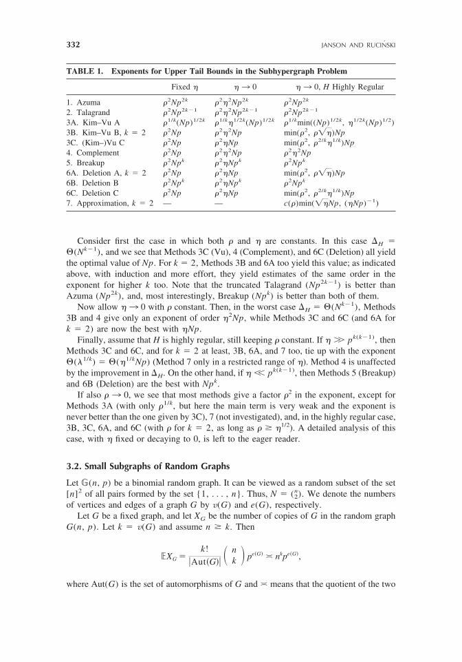
Consider first the case in which both � and � are constants. In this case �H ��(Nk�1), and we see that Methods 3C (Vu), 4 (Complement), and 6C (Deletion) all yieldthe optimal value of Np. For k � 2, Methods 3B and 6A too yield this value; as indicatedabove, with induction and more effort, they yield estimates of the same order in theexponent for higher k too. Note that the truncated Talagrand (Np2k�1) is better thanAzuma (Np2k), and, most interestingly, Breakup (Npk) is better than both of them.

Now allow �3 0 with � constant. Then, in the worst case �H � �(Nk�1), Methods3B and 4 give only an exponent of order �2Np, while Methods 3C and 6C (and 6A fork � 2) are now the best with �Np.

Finally, assume that H is highly regular, still keeping � constant. If � �� pk(k�1), thenMethods 3C and 6C, and for k � 2 at least, 3B, 6A, and 7 too, tie up with the exponent�(�1/k) � �(�1/kNp) (Method 7 only in a restricted range of �). Method 4 is unaffectedby the improvement in �H. On the other hand, if � �� pk(k�1), then Methods 5 (Breakup)and 6B (Deletion) are the best with Npk.

If also � 3 0, we see that most methods give a factor �2 in the exponent, except forMethods 3A (with only �1/k, but here the main term is very weak and the exponent isnever better than the one given by 3C), 7 (not investigated), and, in the highly regular case,3B, 3C, 6A, and 6C (with � for k � 2, as long as � � �1/2). A detailed analysis of thiscase, with � fixed or decaying to 0, is left to the eager reader.

3.2. Small Subgraphs of Random Graphs

Let �(n, p) be a binomial random graph. It can be viewed as a random subset of the set[n]2 of all pairs formed by the set {1, . . . , n}. Thus, N � (2

n). We denote the numbersof vertices and edges of a graph G by v(G) and e(G), respectively.

Let G be a fixed graph, and let XG be the number of copies of G in the random graphG(n, p). Let k � v(G) and assume n � k. Then

�XG �k!

�Aut�G� � nk � pe�G � nkpe�G,

where Aut(G) is the set of automorphisms of G and � means that the quotient of the two

TABLE 1. Exponents for Upper Tail Bounds in the Subhypergraph Problem

Fixed � � 3 0 � 3 0, H Highly Regular

1. Azuma �2Np2k �2�2Np2k �2Np2k

2. Talagrand �2Np2k�1 �2�2Np2k�1 �2Np2k�1

3A. Kim–Vu A �1/k(Np)1/2k �1/k�1/2k(Np)1/2k �1/kmin((Np)1/2k, �1/2k(Np)1/2)3B. Kim–Vu B, k � 2 �2Np �2�2Np min(�2, ��)Np3C. (Kim–)Vu C �2Np �2�Np min(�2, �2/k�1/k)Np4. Complement �2Np �2�2Np �2�2Np5. Breakup �2Npk �2�Npk �2Npk

6A. Deletion A, k � 2 �2Np �2�Np min(�2, ��)Np6B. Deletion B �2Npk �2�Npk �2Npk

6C. Deletion C �2Np �2�Np min(�2, �2/k�1/k)Np7. Approximation, k � 2 — — c(�)min(��Np, (�Np)�1)


sides is bounded from above and below by positive constants. The subgraph counts XG

have received a lot of attention from the pioneering paper by Erdos and Renyi [3] to thepresent day. Bounds for the upper tail (in the more general context of extensions) wereconsidered by Spencer [16], but the breakthrough with general exponential bounds camewith Vu [20].

In this subsection we try our techniques on estimates of the upper tail of XG for threesmall subgraphs: G � K3, G � K4, and G � C4. Throughout we for simplicity assumethat � � 1, i.e., t � �, and leave the case �3 0 to the reader. As a test of how good theseresults are, we compare them with the exponential lower bound on �(XG � (1 � �)�)obtained by Vu [20] (see Sec. 1 for the case K3) (see also [10, (6.2)]). For our three cases,G � K3, G � K4, and G � C4, Vu’s lower bound has the exponent �cn2p2log n,�cn2p3log n and �cn2p2log n, resp.

1. Azuma. Having a choice between vertex and edge exposure, we realize that thelatter is better. Indeed, although the martingale is longer, the Lipschitz con-stants tend to be smaller, as fixing one edge leaves less freedom for creating acopy of a given graph than when fixing just a single vertex. Ignoring constants,for G � K3, G � K4, and G � C4, we have bi � n, bi � n2, and again bi �n2, resp. Thus, the exponents in the estimates are of the order n2p6, n2p12, andn2p8, resp.

2. Talagrand. A truncation similar to that in 3.1.2, restricting the number ofedges to, say, n2p, plus a Chernoff inequality, allows us to apply (7) with bi asfor Azuma and (r) � n2p(max bi)

2. This provides the exponents n2p5,n2p11, and n2p7, resp., thus, by one power of p better than Method 1.

In the case G � K3, for p �� n�1/3, a direct application of the Talagrandinequality, with the certificate being the set of all edges of �(n, p) (they alla.a.s. belong to the copies of K3), yields only the exponent n2p6. For K4 andC4 too, a similar direct approach yields the same exponents as Method 1.

3A. Kim–Vu A. For G � K3, we have k � 3 and �1(X) � max{np2, 1}. Hence,by Theorem 3A,

��XK3 � 2� � n4 �exp �cn1/3p1/6� if p � n�1/ 2

exp �cn1/ 2p1/ 2� otherwise.

Similarly, with k � 6 and �1(X) � max{n2p5, 1},

��XK4 � 2� � n10�exp �cn1/6p1/12� if p � n�2/5

exp �cn1/3p1/ 2� otherwise.

and, with k � 4 and �1(X) � max{n2p3, 1},

��XC4 � 2� � n6�exp �cn1/4p1/8� if p � n�2/3

exp �cn1/ 2p1/ 2� otherwise.

3B, C. Kim–Vu. To apply Theorem 3B even to XK3, we have to use induction. As we

already know, one induction scheme leads to Theorem 3C. It is easily verifiedthat for our three examples, and more generally for any balanced graph G,Theorem 3C applies with k � e(G), � � �1/k, and �j � (C�)1�j/k, provided�1/k � log n, which leads to


��XG � 2� � n exp �c�1/e�G� � n exp �cnv�G/e�Gp�.

For K3, K4, and C4 this yields the exponents np, n2/3p, and np, resp.

The induction used to prove Theorem 3C means in this case adding one edgeat a time to G. However, there are better induction schemes. Vu [18, Theorem3] has shown, using Theorem 3B and an induction adding vertices one by one,the better estimate

��XG � 2� � n exp �c�1/�v�G�1�

for every balanced G. (The induction hypothesis is actually stated moregenerally for extension counts; see [18] for details.) In our three cases, thisyields the exponents n3/ 2p3/ 2, n4/3p2, and n4/3p4/3, resp.

4. Complement. This method works well for dense families �, which is not the casehere. There are �(n6) 3-element subsets of [n]2 and only �(n3) triangles. Thus,� � �(n�3) and so, the exponent in Theorem 4 is �2Np � O( p/n) � o(1).Things get only worse for G � K4 and G � C4.

5. Breakup. By Theorem 5, with �(L) � e(G)�H and �H equal to the Lipschitzconstants from 3.2.1 (Azuma), we obtain exponents n2p3, n2p6, and n2p4, resp.

6. Deletion. First, note that (ignoring constants in the exponent) Theorem 6B gives thesame bounds as Theorem 5, and that Theorem 6C gives the same bounds asTheorem 3C. For K3, K4, and C4 this yields the exponents n2p3, n2p6, and n2p4,resp., for 6B and np, n2/3p, and np, resp., for 6C.Recall that Theorem 6C is based on Theorem 6A and induction; in this case theinduction is over the number of edges in the graph G. Just as for the Kim–Vumethod, there are better induction schemes, and an induction over the number ofvertices in G yields the better estimate

��XG � 2� � n exp �c�1/�v�G�1�

for every balanced G, exactly as for Method 3. (Again the induction hypothesis ismore general; see [10] for details and a general theorem.) In our three cases, thisyields the exponents n3/ 2p3/ 2, n4/3p2, and n4/3p4/3, resp.

There are even more efficient ways to use Theorem 6A, although they so farrequire more effort and ad hoc arguments. First, Theorem 6A can be used directlyfor K3. In this case Y{i} � �iZi, where Zi � Bi(n � 1, p2) is the number of pathsof length 2 between the endpoints of edge i. The Chernoff bound (1) thus yields, see[9, Corollary 2.4], that if �/ 2r � 7np2, then

��Y i� � �/2r � ��Zi � �/2r � exp ��/2r�.

Consequently Theorem 6A yields, for any r such that �/ 2r � 7np2,

��XK3 � 2� � exp �r/9� � N exp ��/2r�.


Choosing r � c��, we obtain

��XK3 � 2� � n2exp �cn3/ 2p3/ 2�,

as obtained above from [10]. This can be slightly improved by choosing instead r �c�� log n, and, using (1) more carefully, leading to

��XK3 � 2� � n2exp �cn3/ 2p3/ 2�log n�

(for details see [10]). Note also that choosing r � �/ 2n in Theorem 6A leads toTheorem 6B, and thus the exponent n2p3, which is better when p �� n�1/3.

For G � K4, as shown in detail in [10], the term �(Y{i} � �/ 2r) can beestimated using a two-fold application of the Chernoff bound (1), which results inthe estimates

��XK4 � 2� � �n2exp �cn2p3� if np2 � 1,n2exp �cn4/3p5/3� otherwise.

(Actually, for p � n�1/ 2��, the exponent can be improved to cn2p3�log n [10].)For p � n�1/ 2, the exponent here differs by only a logarithmic factor from theexponent n2p3log n in Vu’s lower bound, so this estimate is essentially optimal.Here the advantage of the direct Chernoff application over induction is striking.

The case G � C4 was not treated in [10], but a twofold application of theChernoff bound (1) as for K4 yields an essentially optimal bound here too for acertain range of p. In this case Y{i} � �iZi, where Zi is the number of paths oflength 3 between the endpoints of edge i. Note that each such path is determined bythe middle edge and its orientation in the path. Thus, if U is the set of verticesadjacent to at least one of the endpoints of i, and W is the number of edges with bothendpoints in U, then Y{i} � 2W, and thus, for any a � 0,

��Y i� ��

2r� � ��W ��

4r� � ��U� � a � ��Bi�� a2 �, p� �

�

4r�,

where �U� � Bi(n � 2, 2p � p2).

If we choose r and a such that a � 14np � 7��U� and �/4r � 7a2

2p, then by

(1) (see [9, Corollary 2.4]) this yields

��Y i� � �/2r � exp��a � exp��/4r

and hence Theorem 6A yields

��XC4 � 2� � e�cr � � n2 ��e�a � e��/4r.

If p � n�2/3, we choose (for a small c) a � r � cn4/3p and obtain


��XC4 � 2� � n2exp �cn4/3p�, p � n�2/3.

For p � n�2/3, we choose a � cnp1/ 2 and r � cn2p2, and obtain

��XC4 � 2� � n2exp �cn2p2�, p � n�2/3.

Just as for K4, for small p (here p � n�2/3), the obtained exponent matches Vu’slower bound up to a logarithmic factor.

7. Approximation. As we already know, Theorem 7 is never better than Theorem 6A(for � constant as here, at least) (see Remark 2). Here they actually sometimes yieldthe same result. Indeed, for K3 we have R � � � 3��1p2 � �(n4p5), since �1 �n � 2 and �2 � 1, and thus ��2 � 0. We apply the Chernoff bound (1) to Y*1 as forMethod 6A. Since we now need r � R, we see that the essentially optimal choicer � c�� (n3/ 2p3/ 2) used above for Method 6A now is allowed if p � cn�5/7;otherwise, we must be content with the choice r � R. This yields the followingestimates:

��XK3 � 2� � �2 exp �cn3/ 2p3/ 2� if p � n�5/7,exp �c/�np2� otherwise.

For G � K4, Method 7 fares worse. Since �3 � n � 3, we have R � np� �� ,provided that � � 1 to avoid trivialities, and thus r � R implies �/r 3 0 and wedo not get any meaningful bound.

For G � C4 we have, assuming � � 1 and thus np � 1, R � �(�n2p3) ��(n6p7). If p � n�4/5, this allows the essentially optimal choice r � cn2p2 usedfor Method 6A above, and the same double application of the Chernoff bound yieldsagain the optimal bound

��XC4 � 2� � n2exp �cn2p2�, p � n�4/5,

although now for a smaller range of p only. For n�4/5 � p � cn�2/3 we have totake r � R, and can estimate the tail of Y{i} as for Method 6A, now using a �c/np2. We obtain

��XC4 � 2� � n2exp �c/n2p3�, p � n�4/5,

which is meaningful for p �� n�2/3.

Summary of subsection 3.2. The results of this subsection are summarized in Table2 and in Figs. 1–3. A point ( x, y) in the figures signifies a bound of the type c1exp(�c2ny)when p � n�x; in other words, the figures plot the asymptotic value of log�log(bound)�/log n as a function of �log p�/log n. Thus, the bigger y, the better bound. Note that alongthe x-axis, p decreases from constant values at the left end down to 1/n at the right end.The dotted line shows Vu’s lower bound.

We leave the direct comparison of the results obtained by various methods to theanxious reader. Instead, we check how close these estimates get to the lower boundmentioned earlier. For G � K3, none of them achieves it. The nearest are the boundsobtained by Methods 5 and 6 for rather dense graphs and Methods 3, 6 and 7 for sparsergraphs. In the cases G � K4 and G � C4, quite surprisingly, Methods 6 and 7, together


with the double Chernoff argument used above, both achieve the lower bound in somerange of p � p(n). (This can also be achieved by Method 3 [Vu, personal communica-tion].)

Note also that the simple combinatorial Method 5 (Breakup) again beats both Azumaand Talagrand, and together with 6B is the best for rather dense graphs.

TABLE 2. Exponents for Upper Tails in the Small Subgraphs Problem, IgnoringLogarithmic Factors

K3 K4 C4

1. Azuma n2p6 n2p12 n2p8

2. Talagrand n2p5 n2p11 n2p7

3A. Kim–Vu A min(n1/3p1/6, n1/2p1/2) min(n1/6p1/23, n1/3p1/2) min(n1/4p1/8, n1/2p1/2)3B. Kim–Vu B

[20] n3/2p3/2 n4/3p2 n4/3p4/3

3C. (Kim–)Vu C np n2/3p np4. Complement — — —5. Breakup n2p3 n2p6 n2p4

6A. Deletion A[10] max(n3/2p3/2, n2p3) min(n2p3, n4/3p5/3) min(n2p2, n4/3p)

6B. Deletion B n2p3 n2p6 n2p4

6C. Deletion C np n2/3p np7. Approximation min(n3/2p3/2, 1/(np2)) — min(n2p2, 1/n2p3)

Vu’s lower bound n2p2 n2p3 n2p2

Fig. 1. K3.


3.3. How Many Pairs Support Tepees?

Our last example is very special, but still worth mentioning. It shows the strength ofLemma 1 which gave rise to the Deletion Method 6, but so far has not been illustrated byany direct application. In the following problem we would like to obtain an upper bound

Fig. 2. K4.

Fig. 3. C4.


on the upper tail of XC4for p � �(n�1/ 2), which is of the order exp(��(n)), just as Vu’s

lower bound (ignore the logarithm, again). However, none of the Methods 1–7 gives that,and we do not know whether such a bound holds or not. Nevertheless, it turns out that ifwe apply Lemma 1 directly, and instead of proving a genuine bound on the tail allowourselves to discard some edges, we will achieve our task.

The problem itself arose in the study of the width of the threshold for a Ramseyproperty of random graphs [4]. The solution, however, has originated in [15], where theDeletion Method traces back its roots.

Let G be a graph. The base of G, denoted by Base(G), is the set of all pairs of verticesof G with a common neighbor in G. Thus, Base(G) is a graph with the vertex set V(G),but typically not a subgraph of G. It is a subgraph of G2, though.

In [4] the following lemma is needed.

Lemma 4. For every c � 0 and a � 0 there exists a� such that a.a.s. for any (spanning)subgraph F of the random graph �(n, cn�1/ 2) with �E(F)� � acn3/ 2, the graph Base(F)contains at least a�n3 triangles.

In the proof which we only outline here (for details see [5]), an application of a sparseregularity lemma (see [9, Lemma 8.19, p. 216]) to F yields, for a suitably chosen � � 0,the existence of a pair of disjoint subsets of vertices, U and V with an/ 2 � �U� � an,�V� � n/k, where k � K � K(�, a), such that for every W � V, �W� � ��V�, all butat most ��U� vertices of U have each at least

�1 � ��ap�W�/2 � �1 � ��ac��n/2k (18)

neighbors in W, where �� (�, a) � �.The next and last step is to show that a.a.s. every such W induces a subgraph BW of

Base(F)[V] with at least a�( 2�W�) edges, where a� � min{a3c2/ 20, a4/400} does not

depend on �. This will easily imply (see [15, Lemma 2]) that Base(F)[V] itself containsat least a��V�3 triangles, which proves Lemma 4 with a� � a�/K3. The same Lemma 2of [15] determines � � �(a�).

We will underestimate the edges of BW by counting only pairs of vertices of W witha common neighbor in U. So, let H � F[U, W], i.e., H is the bipartite subgraph of F withthe bipartition sets U and W and all the edges of F with one endpoint in U and the otherin W. Then BW � Base(H)[W].

How to count the edges of Base(H)[W]? Let us number the pairs of vertices in W by1, . . . , ( 2

�W�) and denote by xi the number of paths of length 2 in H connecting the verticesof the ith pair (such paths are called tepees in [4]). Set L for the number of those i �{1, . . . , ( 2

�W�)} for which xi � 0, i.e., for the sought number of pairs of vertices of W witha common neighbor in U. Assume that x1, . . . , xL � 0.

Observe that, denoting by du the degree of vertex u � U in H,

�i�1

L

xi � �u�U

�du

2 � and �i�1

L �xi

2� � XC4�H,

where XC4(H) is the number of copies of C4 in H.


If L � ¥i�1L xi/ 2, then by (18) (for � small)

L �1

2 �u�U

�du

2 � �1

33�1 � ��3a3c2�2�n/k2 �

1

20a3c2� �W�

2 � .

Otherwise, by the Cauchy–Schwarz inequality,

�i

�xi

2� � L��i xi /L

2 � ��i xi

2

4L,

and a decent upper bound on XC4(H) will give a lower bound on L and thus on the number

of edges of Base(H)[W].To get back to the genuine random graph not affected by a malicious choice of the

subgraph H, we may bound XC4(H) by XC4

(U, W)—the number of copies of C4 containedin the bipartite subgraph �(n, p)[U, W] of �(n, p) spanned by U and W. Obviously, theexpectation of XC4

(U, W) is equal to ( 2�U�)( 2

�W�) p4 � �(n4p4) � �(n2).To accommodate the number of choices of the sets U and W, which is bounded by 4n,

we would need an upper tail estimate on XC4(U, W) which is close to the lower bound

established by Vu. None of our methods provides such a bound. Fortunately, we may useLemma 1.

Define a random variable Y�k(U, W) � minE0�E(�(n,p)),�E0��kX�E0(U, W), where

X�E0(U, W) is the number of copies of C4 in the subgraph G(n, p)[U, W] � E0. It

follows quickly from Lemma 1 that a.a.s. for all U and W we have

Y�n log n�U, W 2�XC4�U, W � 2��U�2 ��W�

2 �p4 a2�2c4n2

2k2 .

The bottom line of this argument is that even after deleting the edges of E0 � E0(U,W), still all but, say, at most 2��U� vertices of U have each at least (1 � 2��)ap�W�/ 2 �(1 � 2��)ac��n/ 2k neighbors in W. Indeed, as �E0� � n log n, at most, say, n2/3

vertices of U may have each more than n1/3log n edges of E0 incident to them.Let du

0 be the degree of u in H � E0, u � U, and similarly, let xi0 and L0 be

modifications of the previously introduced quantities. Note that �E(Base(H)[W])� � L0

and consider two cases. If L0 � ¥i�1L0

xi0/ 2, then, as before (for � small),

L0 �1

2 �u�U

�du0

2 � �1

20a3c2� �W�

2 � .

If, on the other hand, L0 � ¥i�1L0

xi0/ 2, then

�i

�xi0

2 � � L0��i xi0/L0

2 � �

� �i xi0� 2

4L0


and, so

L0 �

1400 a6c4�4�n/k4

2a2c4�2�n/k2 �a4

400 � �W�2 � ,

as required.

ACKNOWLEDGMENT

This research was partly done during visits of the younger author to Uppsala and of bothauthors to the Department of Computer Science at Lund University; we thank AndrzejLingas for providing the latter opportunity, and Edyta Szymanska for providing her deskand her whiteboard. We further thank Van Vu for sending us unpublished preprints anddrafts.

REFERENCES

[1] G. Bennett, Probability inequalities for the sum of independent random variables, J Am StatAssoc 57 (1962), 33–45.

[2] S. Boucheron, G. Lugosi, and P. Massart, A sharp concentration inequality with applications,Random Struct Alg 16 (2000), 277–292.

[3] P. Erdos and A. Renyi, On the evolution of random graphs, Publ Math Inst Hung Acad Sci 5(1960), 17–61.

[4] E. Friedgut, V. Rodl, A. Rucinski, and P. Tetali, Sharp thresholds for Ramsey properties, inpreparation.

[5] E. Friedgut, Y. Kohayakawa, V. Rodl, A. Rucinski, and P. Tetali, Ramsey games againstone-armed bandit, in preparation.

[6] A. Hajnal and E. Szemeredi, Proof of a conjecture of Erdos, Combinatorial theory and itsapplications, Vol. II, P. Erdos, A. Renyi, and V. T. Sos (Editors), Colloq. Math. Soc. JanosBolyai 4, North-Holland, Amsterdam, 1970, pp. 601–623.

[7] W. Hoeffding, Probability inequalities for sums of bounded random variables, J Am Stat Assoc58 (1963), 13–30.

[8] S. Janson, Poisson approximation for large deviations, Random Struct Alg 1 (1990), 221–230.

[9] S. Janson, T. Łuczak, and A. Rucinski, Random graphs, Wiley, New York, 2000.

[10] S. Janson and A. Rucinski, The deletion method for upper tail estimates, Technical ReportU.U.D.M. 2000:28, Uppsala University, Uppsala, Sweden.

[11] J. H. Kim and V. Vu, Concentration of multivariate polynomials and applications, Combina-torica 20 (2000), 417–434.

[12] C. McDiarmid, On the method of bounded differences, Surveys in combinatorics (Proceedings,Norwich 1989), London Math. Soc. Lecture Note Ser. 141, Cambridge University Press,Cambridge, 1989, pp. 148–188.

[13] C. McDiarmid, Concentration, Probabilistic methods for algorithmic discrete mathematics, M.Habib, C. McDiarmid, J. Ramirez, and B. Reed (Editors), Springer-Verlag, Berlin, 1998, pp.195–248.


[14] V. Rodl and A. Rucinski, Random graphs with monochromatic triangles in every edgecoloring, Random Struct Alg 5(2) (1994), 253–270.

[15] V. Rodl and A. Rucinski, Threshold functions for Ramsey properties, J Am Math Soc 8 (1995),917–942.

[16] J. Spencer, Counting extensions, J Combin Theor A 55 (1990), 247–255.

[17] M. Talagrand, Concentration of measure and isoperimetric inequalities in product spaces, InstHautes Etudes Sci Publ Math 81 (1995), 73–205.

[18] V. H. Vu, On the concentration of multivariate polynomials with small expectation, RandomStruct Alg 16(4) (2000), 344–363.

[19] V. H. Vu, New bounds on nearly perfect matchings in hypergraphs: higher codegrees do help,Random Struct Alg 17(1) (2000), 29–63.

[20] V. H. Vu, A large deviation result on the number of small subgraphs of a random graph,Technical Report MSR-TR-99-90, Combin Probab Comput, to appear.

[21] V. H. Vu, Concentration of non-Lipschitz functions and applications, Random Struct Alg, toappear.


the infamous upper tail

Documents