Page | 1

THE IMPLEMENTATION OF A PORE PRESSURE AND FRACTURE

GRADIENT PREDICTION MODEL FOR THE NORTH SEA CENTRAL JUDY

AND JADE FIELDS

By

JAGADEESH KILAPARTHI

August 2013

A report submitted to the Department of Geography, Environment and

Society, Coventry University in partial fulfilment of the requirements for a

MSc in Petroleum and Environmental Technology

Page | 2

ABSTRACT

The purpose of this project is to implement a pore pressure and fracture gradient prediction strategy for the North Sea Central (Judy and Jade) fields. Measured porosity and pressure data of Judy and Jade fields will be studied and reviewed. This strategy will help to safe drilling, design and completion operations for future wells in these areas.

Judy and Jade field’s data will examine and review on two pore pressure prediction models and one fracture gradient prediction model.

The pore pressure prediction from porosity model was examined primarily in this project to predict the pore pressure and pore pressure gradient. This was new theoretical model of pore pressure prediction, utilizes porosity to predicting the pore pressure. The pore pressure prediction from porosity model allowing normal compaction trendline of porosity to predict the pore pressure.

The Tau model was examined secondarily in this project to predict the pore pressure and pore pressure gradient. This model was derived based on interval velocity and transit time data. Tau model was proposed by Shell, this method dependent on velocity to predict the pore pressure.

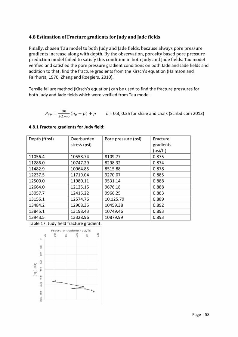
In this project, the fracture pressure and fracture gradient prediction was done based on Kirsch’s solution. The data required for this prediction strategy is overburden stress of formation, pore pressure and Poisson’s ratio. Generally, minimum stress method and tensile failure methods were used in drilling industry. Kirsch’s solution comes under tensile failure method, this prediction strategy delivered simple and accurate results to estimate the fracture pressure gradient.

The two pore pressure prediction strategies examined on available data, that two model pore pressure gradient results compared with the available pore pressure gradient data. Ultimately, Tau model based pore pressure prediction strategy delivered best results. Thus, the Tau model based pore pressure prediction strategy was preferred for future operations in Judy and Jade fields.

Page | 3

RESEARCH DECLARATION

I declare that this dissertation is completely my own work and any use of the others work

has been properly acknowledged. I also confirm that this project has been conducted in

accordance with the University’s ethics guide.

I agree that the research work can be made available as a Reference Document to other

students in the Department of Geography, Environment and Disaster Management.

Signed: ……………………………….. Date: …………………………………

Author’s Name: JAGADEESH KILAPARTHI

Page | 4

ACKNOWLEGEMENTS

I would like to thank Almighty God for making this research work possible and a successful

one. I would also like to express my profound gratitude to my supervisor Ndubuisi Okereke

for his guidance, assistance and at the same time for keeping me centered and able to

remain focused on the goal I set for myself. I am also very grateful to my course director Dr

Babatunde Anifowose, and Augustine Ifebuegu for their support in making sure that this

programme is a successful one.

Completion of this Master programme would not have been possible without the ceaseless

prayers from my parents Appala Paradesi Naidu and Satyavamma throughout this research

project.

My sincere gratitude goes to my friends and well-wishers which are numerous to mention

the names due to word count, thank you for your assistance, sharing knowledge, experience

and time with me. And to everyone who have contributed in one way or the other to the

success of this research but your name has not been mentioned, I say a big thank you to

you.

Page | 5

TABLE OF CONTENTS page numbers

ABSTRACT………………………………………………………………………………………………………………2

RESEARCH DECLARATION………………………………………………………………………………………3

ACKNOWLEDGEMENTS………………………………………………………………………………………….4

LIST OF TABLES………………………………………………………………………………………………………8

LIST OF FIGURES…………………………………………………………………………………………………….9

LIST OF PLOTS……………………………………………………………………………………………………….10

NOMENCLATURE………………………………………………………………………………………………….11

CHAPTER 1……………………………………………………………………………………………………………14

1.0 INTRODUCTION………………………………………………………………………………………………14

1.1. BACKGROUND……………………………………………………………………………………………….14

1.2. AIM………………………………………………………………………………………………………………..15

1.3. OBJECTIVES……………………………………………………………………………………………………15

CHAPTER 2……………………………………………………………………………………………………………16

2.0 LITERATURE REVIEW………………………………………………………………………………………16

2.1. PORE PRESSURE PREDICTION STRATEGIES…………………………………………………….16

2.2. PORE PRESSURE AND PORE PRESSURE GRADIENT…………………………………….....18

2.3. REVIEW OF SOME METHODS OF PORE PRESSURE PREDICTION…………………….20

2.3.1. Pore Pressure Prediction from Resistivity…………………………………………….21

2.3.2. Pore Pressure Prediction from Interval Velocity and Transit Time……….21

2.3.3. Adapted Eaton’s Methods with Depth-Dependent Normal Compaction Trendlines…………………………………………………………………………………………………………….24

2.3.4. New Theoretical Models of Pore Pressure Prediction…………………………..25

2.3.5. Formation Fracture Gradient Prediction Strategy…………………………………28

Page | 6

CHAPTER 3……………………………………………………………………………………………………………………..31

3.0 METHODOLOGY……………………………………………………………………………………………………….31

3.1. Pore Pressure Prediction from Porosity……………………………………………………………………31

3.2. Tau Model………………………………………………………………………………………………………..........31

CHAPTER 4………………………………………………………………………………………………………………………33

4.0 DISCUSSION AND ANALYSIS……………………………………………………………………………………….33

4.1. The Judy Field…………………………………………………………………………………………………………..35

4.2. The Jade Field…………………………………………………………………………………………………………..36

4.3. Analysis of Pore Pressure Prediction from Porosity Model……………………………………….37

4.3.1. Judy Field Pore Pressure Prediction………………………………………………………………..37

4.3.2. Jade Field Pore Pressure Prediction………………………………………………………………..41

4.4. Analysis of Tau Model………………………………………………………………………………………………45

4.4.1. Estimation of Overburden Stress of Judy and Jade field………………………………….45

4.4.2. Estimation of Pore Pressure and Pore Pressure Gradients of Judy and Jade fields……………………………………………………………………………………………………………………………….47

4.5 ANALYSIS OF AVAILABLE DATA………………………………………………………………………………….49 4.5.1 Pore pressure gradients for Judy field……………………………………………………………….50 4.5.2 Pore pressure gradients for Jade field……………………………………………………………….51 4.6 COMPARISON OF PORE PRESSURE GRADIENT RESULTS…………………………………………….52 4.6.1 Comparison of pore pressure gradient plots for Judy field………………………………..52 4.6.2 Comparison of pore pressure gradient plots for Jade field………………………..........54 4.7 COMPARISON OF PORE PRESSURE GRADIENTS INTERMS OF PERCENTAGE…….56 4.7.1 Judy field pore pressure gradients comparison in terms of percentage………………….56

Page | 7

4.7.2 Jade field pore pressure gradients comparison in terms of percentage…………………57 4.8 Estimation of Fracture gradients for Judy and Jade fields…………………………………………58 4.8.1 Fracture gradients for Judy field………………………………………………………………………58 4.8.2 Fracture gradients for Jade field………………………………………………………………………59 4.9 ANALYSIS OF PORE, FRACTURE AND OVERBURDEN GRADIENTS RESULTS……………….60 4.9.1 Judy field all gradients…………………………………………………………………………………….60 4.9.2 Jade field all gradients…………………………………………………………………………………….61 CHAPTER 5…………………………………………………………………………………………………………………….63

5.0 CONCLUSIONS AND RECOMMENDATIONS……………………………………………………………..63

5.1 CONCLUSIONS………………………………………………………………………………………………………..63

5.2 RECOMMENDATIONS…………………………………………………………………………………………….64

REFERENCES…………………………………………………………………………………………………………………65

Page | 8

LIST OF TABLES

Table 1. Judy field depth-porosity data from available diagram.

Table 2. Judy field porosity data from available diagram.

Table 3. Judy field normal porosity data from normal porosity equation.

Table 4. Judy field pore pressure gradient data from pore pressure prediction model.

Table 5. Jade field depth-porosity data from available diagram.

Table 6. Jade field porosity data from available diagram.

Table 7. Jade field normal porosity data from normal porosity equation.

Table 8. Jade field pore pressure gradient data from pore pressure prediction model.

Table 9. Judy field overburden pressure data from available diagram.

Table 10. Jade field overburden pressure data from available diagram.

Table 11. Judy field pore pressure gradient data from Tau model.

Table 12. Jade field pore pressure gradient data from Tau model.

Table 13. Judy field pore pressure gradient data from available diagram.

Table 14. Jade field pore pressure gradient data from available diagram.

Table 15. Judy field pore pressure gradients comparison of available data and Tau model.

Table 16. Jade field pore pressure gradients comparison of available data and Tau model

Table 17. Judy field fracture gradient data from minimum stress method. Table 18. Jade field fracture gradient data from minimum stress method. Table 19. Judy field pore, fracture and overburden gradients data. Table 20. Jade field pore, fracture and overburden gradients data.

Page | 9

TABLE OF FIGURES Figure 1. Hydrostatic pressure, pore pressure, overburden stress, and effective stress in a borehole. Figure 2. Pore pressure gradient, fracture gradient, overburden stress gradient (lithostatic gradient), mud weight, and casing shoes with depth. Figure 3. Schematic porosity (a) and corresponding pore pressure (b) in a sedimentary basin. Figure 4. Study area of Judy and Jade fields. Figure 5. Judy field area. Figure 6. Location of Jade field and its surrounding fields. Figure 7. Judy field porosity percentage. Figure 8. Judy field depth versus porosity graph. Figure 9. Jade field porosity percentage. Figure 10. Judy and Jade field’s lithostatic pressure data. Figure 11. Judy and Jade fields pore pressure data.

Page | 10

LIST OF PLOTS Plot 1. Judy field depth versus porosity. Plot 2. Judy field normal trend line. Plot 3. Judy field pore pressure gradient trend line. Plot 4. Jade field porosity trend line. Plot 5. Jade field normal porosity trend line. Plot 6. Jade field pore pressure gradient trend line. Plot 7. Judy field pore pressure gradient trend line. Plot 8. Jade field pore pressure gradient trend line. Plot 9. Judy field pore pressure gradient trend line. Plot 10. Jade field pore pressure gradient trend line. Plot 11. Judy field pore pressure gradients comparison of available data and porosity based pore pressure prediction model. Plot 12. Judy field pore pressure gradients comparison of available data and Tau model. Plot 13. Jade field pore pressure gradients comparison of available data and porosity based pore pressure prediction model. Plot 14. Jade field pore pressure gradients comparison of available data and Tau model. Plot 15. Judy field fracture gradient trend line. Plot 16. Jade field fracture gradient trend line. Plot 17: Comparison of pore, fracture and overburden gradients of Judy field. Plot 18: Comparison pore, fracture and overburden gradients of Jade field.

Page | 11

NOMENCLATURE pf = the formation fluid pressure (psi); σV = overburden stress (psi); αV = the normal overburden stress gradient (psi/ft); β = the normal fluid pressure gradient (psi/ft); Z = the depth below the mudline or below sea surface (ft); t = the sonic transit time (μs/ft); A, B = the constants; Ppg = the formation pore pressure gradient; OBG = the overburden stress gradient; Png = the hydrostatic pore pressure gradient (normally 0.45 psi/ft or 1.03 MPa/km, dependent on water salinity); R = the shale resistivity obtained from well logging; Rn = the shale resistivity at the normal (hydrostatic) pressure; n = the exponent varied from 0.6 to 1.5, and normally n =1.2; tn = the sonic transit time or slowness in shales at the normal pressure; t = the sonic transit time in shales obtained from well logging; vp = the compressional velocity at a given depth; vml = the compressional velocity in the mudline; tml = the compressional transit time in the mudline; U = the uplift parameter

σmax and vmax = the estimates of the effective stress and velocity at the onset unloading.

pulo = the pore pressure in the unloading case; vm = the sonic interval velocity in the matrix of the shale; vp = the compressional velocity at a given depth; λ = the empirical parameter;

Page | 12

dmax = the depth at which the unloading has occurred; As ,Bs = the fitting constants;

The best fitting parameters in the Gulf of Mexico are As = 1989.6 and Bs = 0.904 (Gutierrez et al, 2006), (for Judy and Jade fields As = 1391.5 and Bs = 0.302 are assumed);

τ = the Tau variable;

C = the constant related to the mudline transit time (normally C = 200 μs/ft);

D = the constant related to the matrix transit time (normally D = 50 μs/ft);

∆t = the compressional transit time (70 μs/ft);

Rn = the shale resistivity in the normal compaction condition; R0 = the shale resistivity in the mudline; b = the constant; Z = the depth below the mudline; R = the measured shale resistivity at depth of Z; R0 = the normal compaction shale resistivity in the mudline; b = the slope of logarithmic resistivity normal compaction trendline; v = the seismic velocity at depth of Z; v0 = the velocity in the ground surface or at the sea floor; k = a constant; tn = the acoustic transit time (μs/m);

tm = the compressional transit time in the shale matrix (with zero porosity); tml = the mudline transit time; c = the constant; ϕ = porosity; ϕ0 = the porosity in the mudline;

Page | 13

Z = the true vertical depth below the mudline; c = the compaction constant in 1/m or 1/ft. a = the stress compaction constant in 1/psi or 1/MPa; Cm = the constant related to the compressional transit time in the matrix and the transit time in the mudline;

∆𝑡𝑓 = the transit time of interstitial fluids;

σmin = the minimum in-situ stress or the lower bound of fracture pressure;

𝑣 = the Poisson's Ratio;

PFG is the formation fracture gradient; Ppg = the formation pore pressure gradient; OBG = the overburden stress gradient; K0 = the effective stress coefficient; σV′ = the maximum effective in-situ stress or effective overburden stress; PFPmax = the upper bound of fracture pressure; σH = the maximum horizontal stress; σmin = the minimum horizontal stress or minimum in-situ stress; σT = the thermal stress induced by the difference between the mud temperature and the formation temperature; T0 = the tensile strength of the rock; PFP = the fracture pressure. Ftbsf = feet below sea floor.

Page | 14

CHAPTER 1 1.0 INTRODUCTION 1.1 BACKGROUND Pore pressure and fracture pressure gradients determinations are vital considerations for the successful planning and drilling of North Sea Central Graben High Pressure High Temperature (HPHT) wells. Understanding of these downhole pressure limitations can have a substantial effect on drilling safety and economics. An exact estimate of the sub-surface pore pressures and fracture gradients is a crucial constraint to safely, economically and efficiently drill the wells required to test and produce oil and natural gas reserves. Pore pressures are simply predicted for normally pressure sediments. It is the prediction of pore pressures for the abnormally pressured (i.e. over pressured) sediments that is more difficult and more important. An understanding of the pore pressure is a requirement of the drilling plan in order to choose proper casing points and design a casing program that will allow the well to be drilled most effectively and maintain well control during drilling and completion operations. Well control events such as formation fluid kicks, lost circulation, surface blowouts and underground blowouts can be avoided with the use of accurate pore pressure and fracture gradient predictions in the design process (Fooshee, S. 2009). The pressure regime of the Central Graben in the North Sea presents a formidable challenge for both exploration drilling and field development. In this area, we apply a practical approach to improve pore-pressure and fracture pressure prediction from seismic velocities derived from amplitude variation with offset (AVO) information. The emphasis is placed on maximising both temporal and lateral resolution of the pressure estimates. Besides assisting exploration well planning, improved resolution may define local pressure variations around a reservoir that assists field appraisal and development. Pressure data from one well in the area is used to calibrate the pressure predictions from seismic velocities and to refine the parameters controlling the predictions. The refined laterally invariant parameters are applied to seismic velocities derived from non- proprietary data over an approximate 500 km2 area in the Central Graben (Hawkins, K. 2004). The variable pressure regime of the Central Graben in the North Sea presents a number of challenges. There are the deep high pressure – high temperature (HPHT) Jurassic and Triassic reservoirs, which are among the most overpressured in the world. Shallower, are the moderately overpressured porous Cretaceous Chalk reservoirs. They are encased in impermeable chalk that prevents accurate pressure measurement or prediction. Above the Chalk are Paleocene reservoirs, which although more normally pressured, exist beneath an overpressured younger Tertiary section. All of these reservoirs require careful adjustment of mud weight: (a) to avoid dangerous blowouts in the HPHT environment, (b) to avoid surprise kicks within the Chalk formations and (c) to limit mud invasion into the Paleocene and some Chalk reservoirs that could hinder appraisal, or even prevent discovery. High pressure – high temperature (HPHT) reservoirs are increasingly becoming the focus of petroleum exploration in the search for additional reserves. The processes leading to the accumulation and preservation of hydrocarbons in these extreme settings are still poorly constrained, especially also with respect to the occurrence of significant porosity at temperatures exceeding 150°C and pressures approaching lithostatic. The processes controlling the evolution of fluid pressure during reservoir burial have been studied by various authors. Overpressure generating mechanisms have been reviewed by Osborne and

Page | 15

Swarbrick (1997), who postulated that disequilibrium compaction is the main mechanism controlling overpressure in the Central Graben. This opinion is supported also by Mann and Mackenzie (1990), although the importance of additional overpressure generation due to gas generation is becoming increasingly acknowledged (Cayley, 1986; Isaksen, 2004; Swarbrick, et al. 2000). 1.2 Aim: The aim of this project to improve the knowledge and verification of pore pressure and fracture gradient prediction models for Judy and Jade fields in North Sea Central HPHT Wells. 1.3 Objectives: The main objectives of this project are: (1) To understanding pore pressure prediction in unconventional plays, is important for executing a safe drilling strategy and for accurate production modelling. (2) To clear understanding of the petro physical data. (3) To review of pore pressure prediction models. (4) To verify and determine suitable pore pressure and fracture gradient model for Judy and Jade fields in North Sea Central HPHT Wells. The purpose of this project is to develop a pore pressure and fracture gradient prediction strategy for the North Sea central HPHT wells, namely the Jade and Judy fields in Quadrant 30, UK North Sea, using petro physical and measured pressure data for wells previously drilled in North Sea central HPHT wells area will be examined and reviewed. The pore pressure and fracture gradient prediction strategy will be useful when designing future drilling and completion operations in the aforementioned area.

Page | 16

CHAPTER 2 2. 0 LITERATURE REVIEW Prediction of Pore-pressure depends greatly on understanding of seismic and well characteristics for instance velocity, resistivity, and density which capture porosity changes during shale compaction under vertical loading. Relationships were developed by Eaton (1975) in the Gulf of Mexico using a moderately simple lithological mix of geologically young sandstones and shale mud rocks at moderately low temperatures. An alternative method using data from the same region was more deterministic—also with vertical stress (e.g., Hottman and Johnson, 1965; Bowers, 1995). Another method using mean stress, developed by Harrold et al. (2000) used comparable sand and shale structures at moderately low temperatures from data in Southeast Asia basins. All the above methodologies can be shown to deliver satisfactory estimate of pore pressure in shale mud rocks in young, quickly placed siliciclastic arrangements, for instance the Baram Delta, Brunei (Tingay et al. 2009) and laterally the West African margin (Swarbrick et al. 2011). The results can be standardised, through cautious consideration to indication for adjacent drainage or adjacent transfer, by means of data from their related reservoir. Though, in higher-temperature environments (e.g., Malay Basin, Hoesni 2004) these approaches be unsuccessful to convey estimates which could be precise sufficient for actual well planning and safe drilling. The foremost determination of this literature review was accomplished to improvement understanding of diverse pore pressure and fracture gradient estimate approaches in an exertion to find the finest approach for this area. This review, though, is not fully thorough by means of there are a massive numeral of approaches that have been established meanwhile the middle of the twentieth century. This review is inadequate to a limited pore pressure estimate approaches and two fracture gradient estimate approaches. However realising the several pore pressure and fracture gradient estimate approaches, a determination was made to validate or conclude the petro physical data essential for a comprehensive estimate approach. Those approaches will also be comprised in the literature review. 2.1 PORE PRESSURE AND FRACTURE PRESSURE PREDICTION STRATEGIES Overpressures can be made through various mechanism, for instance compaction imbalance means Undercompaction, generation of hydrocarbons, cracking process of gas, aqua thermal expansion, lateral stress in formations, transformation of minerals (i.e., illitiza-tion), and process of osmosis, hydrostatic column and resistance of hydrocarbons ( Swarbrick and Osborne, 1998; Gutierrez et al. 2006). In all cases where compaction disequilibrium has been calculated to be the main reason of over pressuring, the time of life of the rocks is geologically young. Instances of regions where compaction disequilibrium is named as the crucial cause of abnormal pressure include the U.S. Gulf Coast, Alaska Cook Inlet, Beaufort Sea, Mackenzie Delta, North Sea, Adriatic Sea, Niger Delta, Mahakam Delta, the Nile Delta, Malay Basin, Eastern Venezuelan Basin (Trinidad) and the Pot war Plateau of Pakistan ( Powley, 1990; Burrus, 1998; Heppard et al. 1998; Law and Spencer, 1998; Nelson & Bird 2005; Morley et al. 2011). In these regions, the unusually pressured rocks are mostly situated in Tertiary and late Mesozoic sedimentary formations, the depositional setting is dominantly deltaic, and the lithology is dominantly shale.

Page | 17

Abnormal formation compaction such as compaction disequilibrium, Undercompaction are main causes for abnormal pore pressure. Pore fluid eviction and compression of formation porosity occurred generally where deposits compressed. The foremost cause of fluid barring is overburden pressure increasing with depth. The rate of sedimentation and normal compaction are vice versa, means if normal compaction rises, the rate of sedimentation is becoming slow. Fluids expel ability effects the equilibrium between overburden rise and volume of pore fluid reduction ( Mouchet & Mitchell 1989). The hydrostatic pore pressure generation depends on the normal compaction. Though, quick burial hints to quicker exclusion of fluids in answer to quickly growing overburden stress. At what time the deposits recede quickly, or else the formation has enormously little permeability, fluids in the deposits can only be incompletely ejected. That continued fluid in the pores of the deposits essential backing them or portion of the heaviness of excessively deposits, producing the pressure of pore fluid rises, unusually great pore pressure. Two pore pressure prediction strategies and one fracture gradient prediction strategy will be reviewed and applied to the available data. The two pore pressure prediction strategies require petro physical data, specifically formation resistivity or conductivity, to predict pore pressures. The fracture gradient prediction strategy requires an accurate estimate of pore Pressure. The first pore pressure prediction strategy reviewed was developed by seismic velocity pore pressure prediction model. This strategy utilizes a series of geologic age specific overlays, which indicate the normally pressured compaction trend lines for the respective geologic age. After plotting the observed resistivity/conductivity data on the geologic age specific overlay, the pore pressures can be predicted. A simple calibration of the data was required to establish the normal pressure trend line implemented in this method. The second pore pressure prediction strategy reviewed was developed by Ben Eaton (1975). Eaton developed a simple relationship that will predict the pore pressure knowing the normally pressured compaction trend line, the observed resistivity/conductivity data and a relationship for the overburden stress versus depth. The fracture pressure prediction strategy reviewed was also developed by Ben Eaton (1975). The data required for this prediction strategy is formation overburden stress, pore pressure and Poisson’s ratio of the formation. A relationship for the overburden stress and Poisson’s ratio can be developed based on field data, or one of Eaton’s generalized relationships can be used.

Page | 18

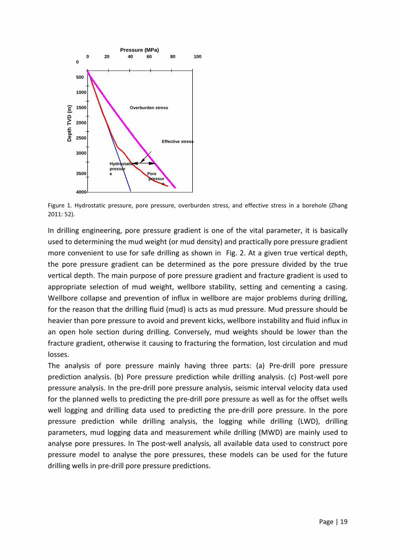
2.2 PORE PRESSURE AND PORE PRESSURE GRADIENT Estimation of Pore pressure plays key role in the planning of well drilling and for geomechanical, geological analysis. Pore pressure means the fluids exerted pressures in the pore spaces in porous formations. Some types of Pore pressures are hydrostatic pressure, abnormal pressure and overburden pressure, it be changes from hydrostatic pressure, to over burden pressure (48% to 95% of the overburden stress). Hydrostatic pressure is normally called normal pressure, if the pore pressure is lesser or upper than the hydrostatic pressure (normal pore pressure), it is called abnormal pore pressure and when pore pressure more than hydrostatic pressure (normal pore pressure), it is called overburden pressure. Pore pressure prediction’s basic theory derived from Terzaghi's and Biot's effective stress law ( Biot. 1941; Terzaghi et al. 1996). This fundamental theory represents the formation pore pressure is a function of overburden stress and effective stress. The Terzaghi's and Biot's effective stress law generated a correlation to explain the relationship of overburden stress, effective vertical stress and pore pressure. It can be expressed in the following form: p = (σV −σe) / α (1) Where pore pressure (p); overburden stress (σV); vertical effective stress (σe); and Biot effective stress coefficient (α). It is usually assumed α=1 in geo pressure community. Pore pressure calculation from equation (1) depends on overburden stress and effective stress. When these two stresses known, can be calculated pore pressure. Bulk density logs and well log data, for instance resistivity, sonic travel time/ velocity, bulk density and drilling parameters (e.g., D exponent) generally used to generate the data of overburden stress, effective stress. The hydrostatic pressure, vertical effective stress, overburden stress and formation pore pressure profiles demonstrated with the true vertical depth (TVD) in Fig. 1 of a characteristic oil and gas exploration well. The pore pressure trend line with true vertical depth in these fields are comparable to several sedimentary young fields where over pore pressure is come across at depth. Pore pressure is hydrostatic, that indicating continuous unified column of formation pore fluid spreads from surface to depth at moderately low depths (less than 2000 m). At more than 2000 m depths, pore pressure increases with true vertical depth quickly and overpressure is started, This represents the deeper formations hydraulically remote from shallower formations. If pore pressure value reaches by 3800 m near to the overburden stress value, that state mentioned as hard overpressure. The subtraction value of pore pressure (p) from overburden stress (σV) conventionally defined as effective stress (σe) as shown in Fig. 1. The overpressure increase represents the reduction of the effective stress.

Page | 19

Pressure (MPa) 0 20 40 60 80 100

0

500

1000

TVD

(m)

1500 Overburden stress

2000

Dept

h 2500

Effective stress

3000

3500 Hydrostatic

pressur

e Pore

pressur

e

4000

Figure 1. Hydrostatic pressure, pore pressure, overburden stress, and effective stress in a borehole (Zhang 2011: 52). In drilling engineering, pore pressure gradient is one of the vital parameter, it is basically used to determining the mud weight (or mud density) and practically pore pressure gradient more convenient to use for safe drilling as shown in Fig. 2. At a given true vertical depth, the pore pressure gradient can be determined as the pore pressure divided by the true vertical depth. The main purpose of pore pressure gradient and fracture gradient is used to appropriate selection of mud weight, wellbore stability, setting and cementing a casing. Wellbore collapse and prevention of influx in wellbore are major problems during drilling, for the reason that the drilling fluid (mud) is acts as mud pressure. Mud pressure should be heavier than pore pressure to avoid and prevent kicks, wellbore instability and fluid influx in an open hole section during drilling. Conversely, mud weights should be lower than the fracture gradient, otherwise it causing to fracturing the formation, lost circulation and mud losses. The analysis of pore pressure mainly having three parts: (a) Pre-drill pore pressure prediction analysis. (b) Pore pressure prediction while drilling analysis. (c) Post-well pore pressure analysis. In the pre-drill pore pressure analysis, seismic interval velocity data used for the planned wells to predicting the pre-drill pore pressure as well as for the offset wells well logging and drilling data used to predicting the pre-drill pore pressure. In the pore pressure prediction while drilling analysis, the logging while drilling (LWD), drilling parameters, mud logging data and measurement while drilling (MWD) are mainly used to analyse pore pressures. In The post-well analysis, all available data used to construct pore pressure model to analyse the pore pressures, these models can be used for the future drilling wells in pre-drill pore pressure predictions.

Page | 20

Gradient (SG) 1.0 1.2 1.4 1.6 1.8 2.0 2.2 2.4

0

500 Lithostatic gradient

1000

(m)

1500 Fracture

gradient

TVD

2000 Casing

Dep

th

2500 Mud weight

3000

3500 Pore pressure

gradient

4000

Figure 2. Pore pressure gradient, fracture gradient, overburden stress gradient (lithostatic gradient), mud weight, and casing shoes with depth (Zhang 2011: 52) 2.3 REVIEW OF SOME METHODS OF PORE PRESSURE PREDICTION The first pore pressure prediction approach was derived by Hottmann and Johnson (1965), they were derived this approach for shale formations based on well log data such as velocity, resistivity and acoustic travel time. Their approach derived and initiated in Upper Texas and Southern Louisiana Gulf Coast of Miocene and Oligocene shale formations, they specified one specification was related to porosity and depth. If depth increases, the porosity decreases means decreasing of porosity is function of depth. The relationship between porosity and depth was called normal compaction trend, this tendency signifies normal compaction trend was function of depth and fluid pressure in burial depths showed in normal trend is called hydrostatic pressure. The normal compaction trend’s subsequent data points are deviate, when the abnormal compaction intervals are penetrated. If fluid pressure in formation is abnormally high, the intervals of abnormal compaction are resisted the porosity of shale at abnormally high depths. Hottmann and Johnson (1965), Gardner et al. (1974) were proposed an equation to predict the formation pore pressure based on analysing the data. That can be written as in the following form:

Ƿf = σv - [(σv – β) (A1 – B1 ln ∆t)3 ÷ Z2 ] (2)

Where, the formation fluid pressure (pf) expressed in psi; the overburden stress (σV) expressed in psi; the normal overburden stress gradient (αV) expressed in psi/ft; the normal fluid pressure gradient (β) expressed in psi/ft; the depth (Z) expressed in ft; the sonic transit time (t) expressed in μs/ft; A, B are the constants, A1 =82,776 and B1 =15,695.

Afterward, many pore pressure prediction methods, models and empirical equations were obtained based on well logging data such as: resistivity, interval velocity, sonic transit time and other data. In the below sections explained and discussed the some normally used pore pressure prediction methods based on properties of shale.

Page | 21

2.3.1 Pore pressure prediction from resistivity

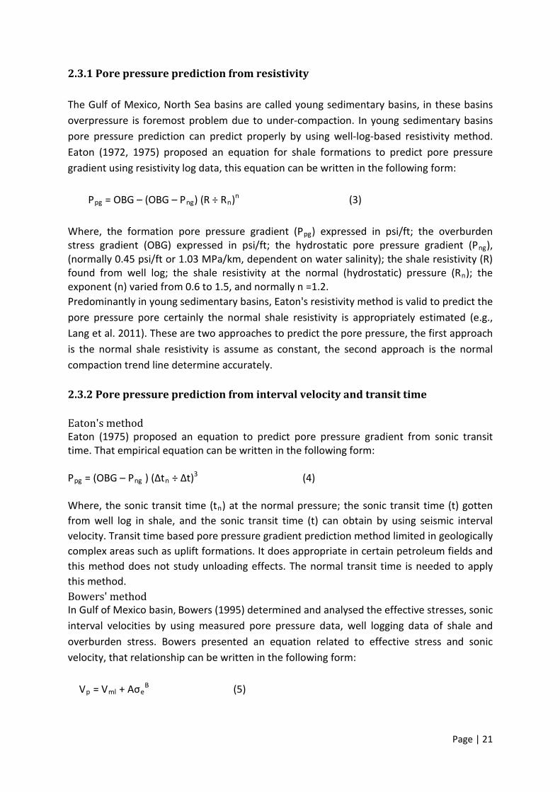
The Gulf of Mexico, North Sea basins are called young sedimentary basins, in these basins overpressure is foremost problem due to under-compaction. In young sedimentary basins pore pressure prediction can predict properly by using well-log-based resistivity method. Eaton (1972, 1975) proposed an equation for shale formations to predict pore pressure gradient using resistivity log data, this equation can be written in the following form:

Ppg = OBG – (OBG – Png) (R ÷ Rn)n (3)

Where, the formation pore pressure gradient (Ppg) expressed in psi/ft; the overburden stress gradient (OBG) expressed in psi/ft; the hydrostatic pore pressure gradient (Png), (normally 0.45 psi/ft or 1.03 MPa/km, dependent on water salinity); the shale resistivity (R) found from well log; the shale resistivity at the normal (hydrostatic) pressure (Rn); the exponent (n) varied from 0.6 to 1.5, and normally n =1.2. Predominantly in young sedimentary basins, Eaton's resistivity method is valid to predict the pore pressure pore certainly the normal shale resistivity is appropriately estimated (e.g., Lang et al. 2011). These are two approaches to predict the pore pressure, the first approach is the normal shale resistivity is assume as constant, the second approach is the normal compaction trend line determine accurately. 2.3.2 Pore pressure prediction from interval velocity and transit time Eaton's method Eaton (1975) proposed an equation to predict pore pressure gradient from sonic transit time. That empirical equation can be written in the following form: Ppg = (OBG – Png ) (∆tn ÷ ∆t)3 (4) Where, the sonic transit time (tn) at the normal pressure; the sonic transit time (t) gotten from well log in shale, and the sonic transit time (t) can obtain by using seismic interval velocity. Transit time based pore pressure gradient prediction method limited in geologically complex areas such as uplift formations. It does appropriate in certain petroleum fields and this method does not study unloading effects. The normal transit time is needed to apply this method. Bowers' method In Gulf of Mexico basin, Bowers (1995) determined and analysed the effective stresses, sonic interval velocities by using measured pore pressure data, well logging data of shale and overburden stress. Bowers presented an equation related to effective stress and sonic velocity, that relationship can be written in the following form:

Vp = Vml + Aσe

B (5)

Page | 22

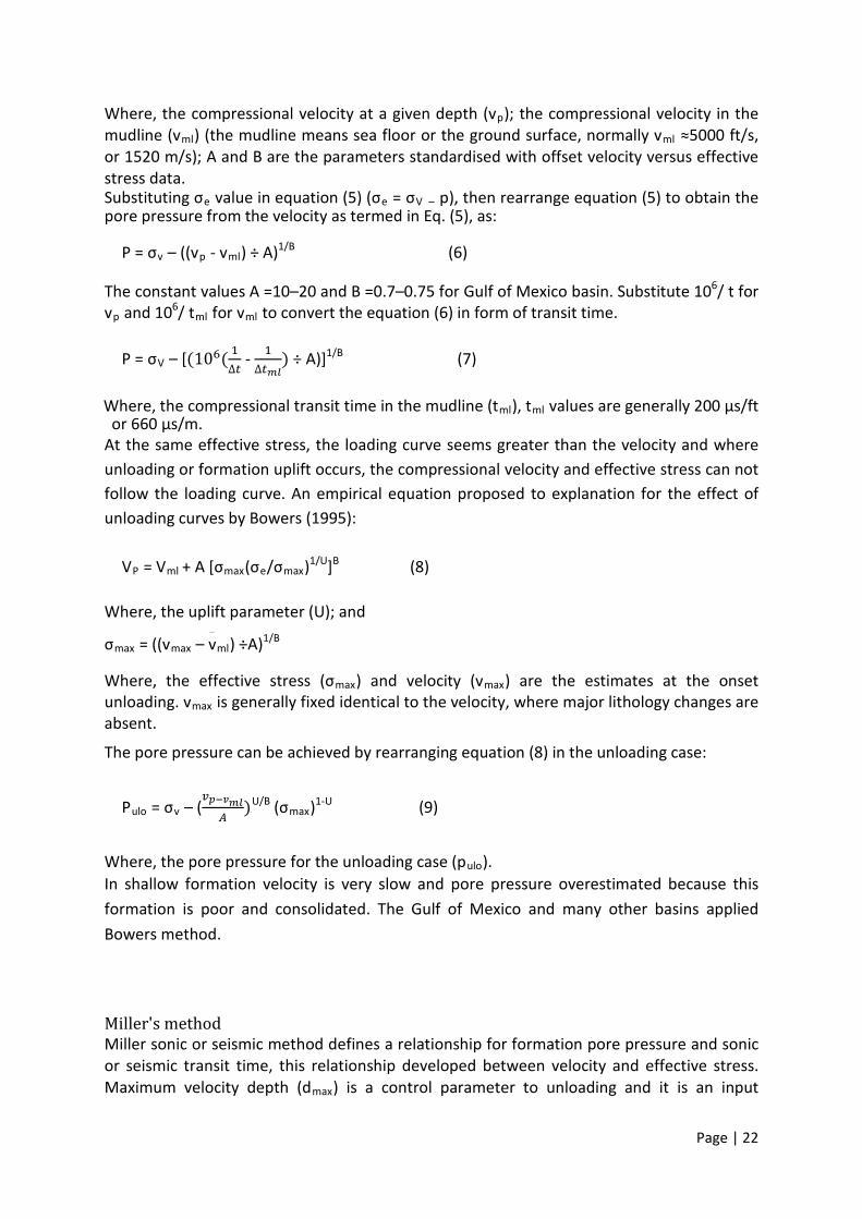
Where, the compressional velocity at a given depth (vp); the compressional velocity in the mudline (vml) (the mudline means sea floor or the ground surface, normally vml ≈5000 ft/s, or 1520 m/s); A and B are the parameters standardised with offset velocity versus effective stress data. Substituting σe value in equation (5) (σe = σV – p), then rearrange equation (5) to obtain the pore pressure from the velocity as termed in Eq. (5), as:

P = σv – ((vp - vml) ÷ A)1/B (6)

The constant values A =10–20 and B =0.7–0.75 for Gulf of Mexico basin. Substitute 106/ t for vp and 106/ tml for vml to convert the equation (6) in form of transit time.

P = σV – [(106( 1

∆𝑡 - 1∆𝑡𝑚𝑙

) ÷ A)]1/B (7)

Where, the compressional transit time in the mudline (tml), tml values are generally 200 μs/ft

or 660 μs/m. At the same effective stress, the loading curve seems greater than the velocity and where unloading or formation uplift occurs, the compressional velocity and effective stress can not follow the loading curve. An empirical equation proposed to explanation for the effect of unloading curves by Bowers (1995):

VP = Vml + A [σmax(σe/σmax)1/U]B (8)

Where, the uplift parameter (U); and σmax = ((vmax – vml) ÷A)1/B Where, the effective stress (σmax) and velocity (vmax) are the estimates at the onset unloading. vmax is generally fixed identical to the velocity, where major lithology changes are absent. The pore pressure can be achieved by rearranging equation (8) in the unloading case:

Pulo = σv – (𝑣𝑝−𝑣𝑚𝑙

𝐴)P

U/B (σmax)1-U (9)

Where, the pore pressure for the unloading case (pulo). In shallow formation velocity is very slow and pore pressure overestimated because this formation is poor and consolidated. The Gulf of Mexico and many other basins applied Bowers method.

Miller's method Miller sonic or seismic method defines a relationship for formation pore pressure and sonic or seismic transit time, this relationship developed between velocity and effective stress. Maximum velocity depth (dmax) is a control parameter to unloading and it is an input

Page | 23

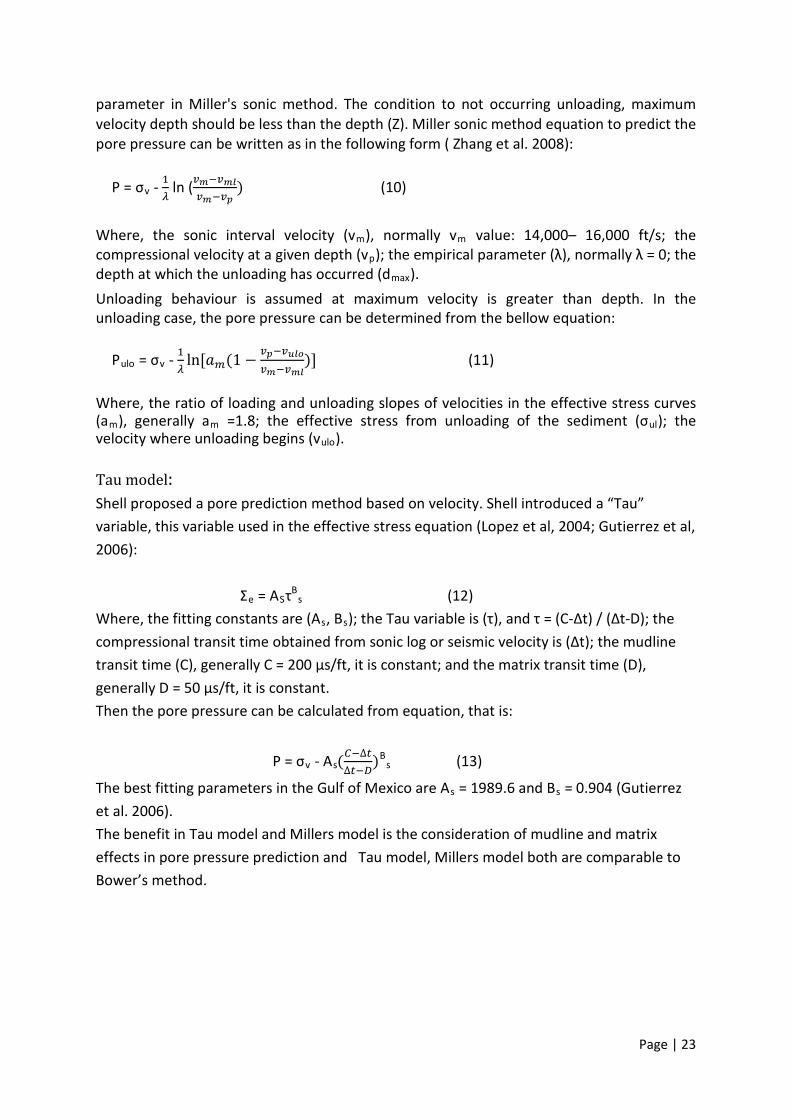
parameter in Miller's sonic method. The condition to not occurring unloading, maximum velocity depth should be less than the depth (Z). Miller sonic method equation to predict the pore pressure can be written as in the following form ( Zhang et al. 2008):

P = σv - 1

𝜆 ln (𝑣𝑚−𝑣𝑚𝑙

𝑣𝑚−𝑣𝑝) (10)

Where, the sonic interval velocity (vm), normally vm value: 14,000– 16,000 ft/s; the compressional velocity at a given depth (vp); the empirical parameter (λ), normally λ = 0; the depth at which the unloading has occurred (dmax). Unloading behaviour is assumed at maximum velocity is greater than depth. In the unloading case, the pore pressure can be determined from the bellow equation:

Pulo = σv - 1

𝜆ln[𝑎𝑚(1 − 𝑣𝑝−𝑣𝑢𝑙𝑜

𝑣𝑚−𝑣𝑚𝑙)] (11)

Where, the ratio of loading and unloading slopes of velocities in the effective stress curves (am), generally am =1.8; the effective stress from unloading of the sediment (σul); the velocity where unloading begins (vulo). Tau model: Shell proposed a pore prediction method based on velocity. Shell introduced a “Tau” variable, this variable used in the effective stress equation (Lopez et al, 2004; Gutierrez et al, 2006): Σe = ASτB

s (12) Where, the fitting constants are (As, Bs); the Tau variable is (τ), and τ = (C-∆t) / (∆t-D); the compressional transit time obtained from sonic log or seismic velocity is (∆t); the mudline transit time (C), generally C = 200 μs/ft, it is constant; and the matrix transit time (D), generally D = 50 μs/ft, it is constant. Then the pore pressure can be calculated from equation, that is:

P = σv - As(𝐶−∆𝑡∆𝑡−𝐷

)P

Bs (13)

The best fitting parameters in the Gulf of Mexico are As = 1989.6 and Bs = 0.904 (Gutierrez et al. 2006). The benefit in Tau model and Millers model is the consideration of mudline and matrix effects in pore pressure prediction and Tau model, Millers model both are comparable to Bower’s method.

Page | 24

2.3.3 Adapted Eaton's methods with depth-dependent normal compaction trendlines Eaton's resistivity method with depth-dependent normal compaction trendline: Eaton's primary equation in hydrostatic pore pressure case, is challenging to define the resistivity or normal resistivity of shale. A new approach to determine the normal resistivity of shale is assumed as constant of normal shale resistivity. Though, the normal resistivity of shale is a constraint of formation depth and it is in many cases not constant. Therefore for the pore pressure prediction the normal compaction trendline should be require to determine. Measured resistivity is a function of burial depth, based on this a relationship developed between burial depth and measured resistivity for normal pressured formations. The resistivity’s normal compaction trend line equation can be following in the form:

Ln Rn = ln Ro + bZ or Rn = R0ebZ (14)

Where, In the case of normal compaction, the shale resistivity is (Rn); the resistivity of shale in the sea floor is (R0); the constant is (b); and the depth below the sea floor is (Z). The Eaton's resistivity equation can be stated by substituting equation (14) into pFPmax = 2σmin – p in the following equation:

Ppg = OBG – (OBG – Png) ( 𝑅

𝑅0𝑒𝑏𝑍)P

n (15)

Where, at depth Z, the measured shale resistivity is (R); in the sea floor the normal compaction shale resistivity is (R0); the slope of logarithmic resistivity normal compaction trendline is (b).

Eaton's velocity method with depth-dependent normal compaction trendline: In the subsurface formations the velocity rises with burial depth. The phenomenon predicted by Slotnick (1936) was that represents the compressional velocity is depends on depth. Thus, the travel time’s normal compaction trendline must be a constraint of depth. Slotnick (1936) proposed a linear relationship of seismic velocity’s first and easy normal compaction trendline in the below equation:

V = V0 + kZ (16)

Where, at depth Z, the seismic velocity is (v); the velocity at the sea floor is (v0); constant is (k). The normal pressured velocity relationship proposed by Sayers et al. (2002) to predict the pore pressure. In Carnarvon Basin established a relationship for depth dependent shale acoustic travel time. This exponential relationship established from 17 normally pressured

Page | 25

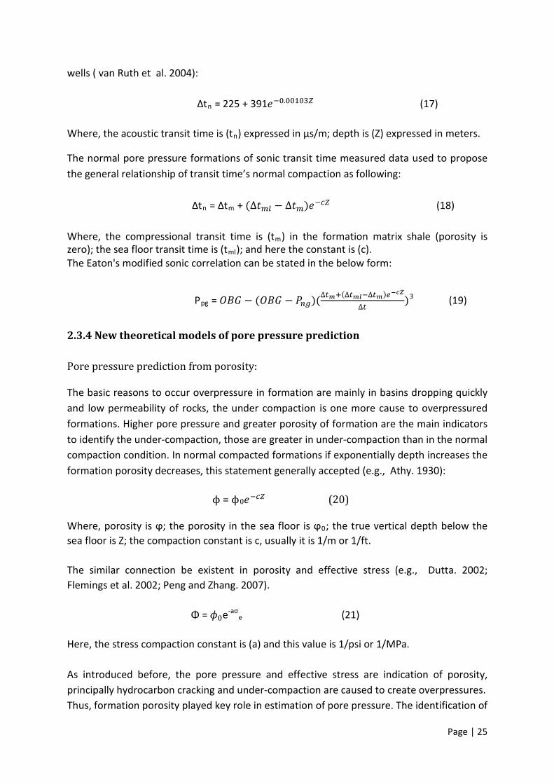
wells ( van Ruth et al. 2004): ∆tn = 225 + 391𝑒−0.00103𝑍 (17)

Where, the acoustic transit time is (tn) expressed in μs/m; depth is (Z) expressed in meters. The normal pore pressure formations of sonic transit time measured data used to propose the general relationship of transit time’s normal compaction as following:

∆tn = ∆tm + (∆𝑡𝑚𝑙 − ∆𝑡𝑚)𝑒−𝑐𝑍 (18)

Where, the compressional transit time is (tm) in the formation matrix shale (porosity is zero); the sea floor transit time is (tml); and here the constant is (c). The Eaton's modified sonic correlation can be stated in the below form:

Ppg = 𝑂𝐵𝐺 − (𝑂𝐵𝐺 − 𝑃𝑛𝑔)(∆𝑡𝑚+(∆𝑡𝑚𝑙−∆𝑡𝑚)𝑒−𝑐𝑍

∆𝑡)P

3 (19)

2.3.4 New theoretical models of pore pressure prediction Pore pressure prediction from porosity: The basic reasons to occur overpressure in formation are mainly in basins dropping quickly and low permeability of rocks, the under compaction is one more cause to overpressured formations. Higher pore pressure and greater porosity of formation are the main indicators to identify the under-compaction, those are greater in under-compaction than in the normal compaction condition. In normal compacted formations if exponentially depth increases the formation porosity decreases, this statement generally accepted (e.g., Athy. 1930): ϕ = ϕ0𝑒−𝑐𝑍 (20) Where, porosity is ϕ; the porosity in the sea floor is ϕ0; the true vertical depth below the sea floor is Z; the compaction constant is c, usually it is 1/m or 1/ft. The similar connection be existent in porosity and effective stress (e.g., Dutta. 2002; Flemings et al. 2002; Peng and Zhang. 2007). Φ = 𝜙0e-aσ

e (21) Here, the stress compaction constant is (a) and this value is 1/psi or 1/MPa. As introduced before, the pore pressure and effective stress are indication of porosity, principally hydrocarbon cracking and under-compaction are caused to create overpressures. Thus, formation porosity played key role in estimation of pore pressure. The identification of

Page | 26

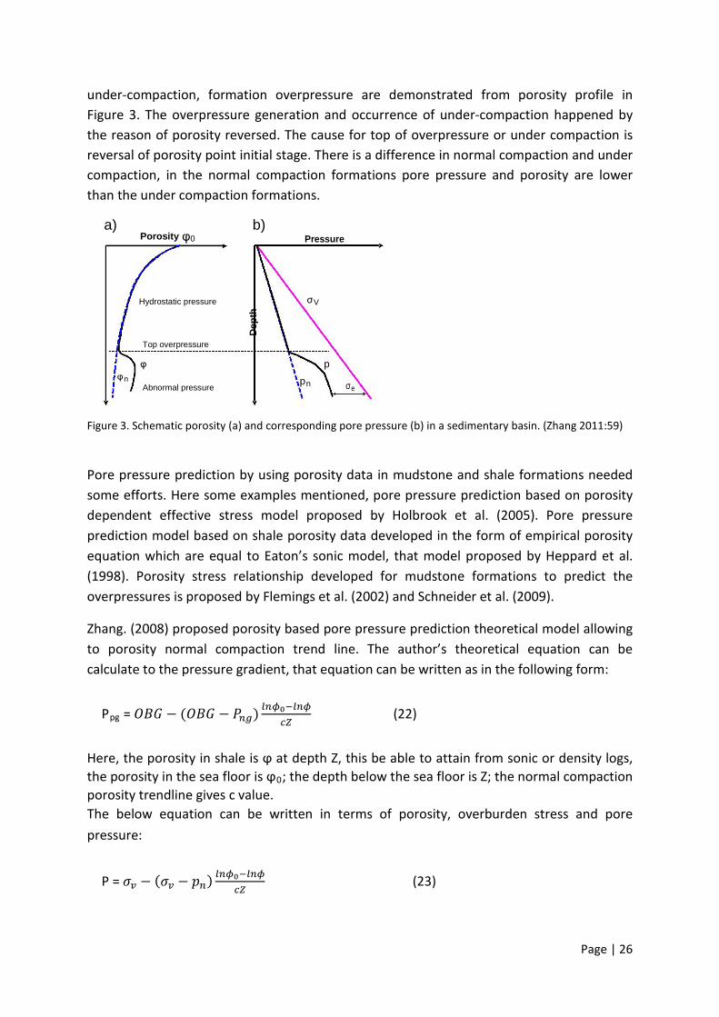
under-compaction, formation overpressure are demonstrated from porosity profile in Figure 3. The overpressure generation and occurrence of under-compaction happened by the reason of porosity reversed. The cause for top of overpressure or under compaction is reversal of porosity point initial stage. There is a difference in normal compaction and under compaction, in the normal compaction formations pore pressure and porosity are lower than the under compaction formations.

a) Porosity φ0

b) Pressure

Hydrostatic pressure σV

Dep

th

Top overpressure

φ p

φn pn σe Abnormal pressure

Figure 3. Schematic porosity (a) and corresponding pore pressure (b) in a sedimentary basin. (Zhang 2011:59) Pore pressure prediction by using porosity data in mudstone and shale formations needed some efforts. Here some examples mentioned, pore pressure prediction based on porosity dependent effective stress model proposed by Holbrook et al. (2005). Pore pressure prediction model based on shale porosity data developed in the form of empirical porosity equation which are equal to Eaton’s sonic model, that model proposed by Heppard et al. (1998). Porosity stress relationship developed for mudstone formations to predict the overpressures is proposed by Flemings et al. (2002) and Schneider et al. (2009). Zhang. (2008) proposed porosity based pore pressure prediction theoretical model allowing to porosity normal compaction trend line. The author’s theoretical equation can be calculate to the pressure gradient, that equation can be written as in the following form:

Ppg = 𝑂𝐵𝐺 − (𝑂𝐵𝐺 − 𝑃𝑛𝑔) 𝑙𝑛𝜙0−𝑙𝑛𝜙𝑐𝑍

(22)

Here, the porosity in shale is ϕ at depth Z, this be able to attain from sonic or density logs, the porosity in the sea floor is ϕ0; the depth below the sea floor is Z; the normal compaction porosity trendline gives c value. The below equation can be written in terms of porosity, overburden stress and pore pressure:

P = 𝜎𝑣 − (𝜎𝑣 − 𝑝𝑛) 𝑙𝑛𝜙0−𝑙𝑛𝜙𝑐𝑍

(23)

Page | 27

The above equation can be calculated pore pressure that is depth dependent equation to calculate the pore pressure. This is the basic difference to above equation and other porosity-pore pressure equations. In addition to that, porosity normal compaction trend line is indicator of depth. The indication of formation overpressured, if the porosity (ϕ) is greater at chosen depth compared with the normal porosity (ϕn) at the same chosen depth, this is called the formation is overpressured. The below equation used to generate the normal compaction porosity trendline for overpressured formations:

Φn = ϕ0𝑒−𝑐𝑍 (24)

Pore pressure prediction from transit time or velocity:

Density logs, sonic logs and seismic interval velocity data are required to collect Porosity data. Raiga-Clemenceau et al. (1988) proposed an equation to generate porosity by using transit time or compressional velocity. Porosity can be calculated from the following equation:

𝜙 = 1 − (∆𝑡𝑚∆𝑡

)P

1/x (25)

Here, the exponent (x) can be obtained from the data. Issler (1992) proposed exponent x value as 2.19 at fixed transit time value tm =67 μs/ft for Mackenzie Delta of northern Canada. From velocity or compressional transit time, the pore pressure calculated by rearranging equation (25) and (22):

𝑝𝑝𝑔 = 𝑂𝐵𝐺 − (𝑂𝐵𝐺 − 𝑃𝑛𝑔)𝐶𝑚−ln [1−�∆𝑡𝑚∆𝑡 �

1𝑥]

𝑐𝑍 (26)

Here, the compressional transit time in the matrix, the transit time in the sea floor is (Cm). Where, it can be written as Cm =ln[1 − ( tm/ tml)1/x]. Wyllie et al. (1956) proposed an empirical equation for porosity estimation. 𝜙 = ∆𝑡−∆𝑡𝑚

∆𝑡−∆𝑡𝑚 (27)

Here, the transit time of fluid is ∆𝑡𝑓 The pore pressure gradient and pore pressure are calculated from Wyllie's porosity-transit time equations. These equations can be written in following correlations:

Page | 28

𝑝𝑝𝑔 = 𝑂𝐵𝐺 − (𝑂𝐵𝐺 − 𝑃𝑛𝑔) ln(∆𝑡𝑚𝑙−∆𝑡𝑚)−ln (∆𝑡−∆𝑡𝑚)

𝑐𝑍 (28)

𝑝 = 𝜎𝑣 − (𝜎𝑣 − 𝑝𝑛) ln(∆𝑡𝑚𝑙−∆𝑡𝑚)−ln (∆𝑡−∆𝑡𝑚)

𝑐𝑍 (29)

The below equation can be used to calculate the normal compaction trendline of the transit time:

∆𝑡𝑛 = ∆𝑡𝑚 + (∆𝑡𝑚𝑙 − ∆𝑡𝑚)𝑒−𝑐𝑍 (30)

The advantages of this model is at higher depths normal transit time reaches the matrix transit time because of normal compaction trend, this method physically approved Chapman (1983). The main difference to other methods and this method, in this method normal compaction trendline is used and compaction mechanism better for sediments. The additional benefits of this method is depth dependent to calculate pore pressures and consideration of matrix, mudline transit time effects. 2.3.5 Formation Fracture Gradient Prediction Strategy Formation fracture pressure mandatory to crack the formation and the disadvantage of fracture pressure is mud losses, this is caused by high fracture pressure. If fracture pressure is high the mud entered from wellbore to made Fracture. Normally, fracture pressures are calculated by using models, however fracture gradients can be calculated by fracture pressure divided with the true vertical depth (TVD). The fracture gradient means maximum mud weight and the main advantage of fracture gradient generally used in three fields, which are drilling planning, while drilling and mud weight design. The wrong formation fracture gradient estimation leads to tensile failure, mud losses or lost circulation, these can be happened in the case of mud weight value is greater than the formation fracture gradient. Formation fracture pressure measured by using many tests and approaches, such as downhole leak-off test (LOT) and the minimum stress method, tensile failure method. In drilling industry basically used two methods, that are (1) the minimum stress method. (2) The tensile failure method. Minimum stress for lower bound of fracture gradient: The tensile strength of rock property does not discuss in the minimum stress method, it only discuss about the pressure to fracture the formation and extend the already fractured the formation. Hence, the lower bound of fracture pressure signifies the minimum stress. The

Page | 29

fracture closure pressure is naturally equal to the minimum stress, this principal detected in leak-off test resulting the breakdown pressure ( Zhang et al. 2008). Hubbert and Willis (1957), Eaton (1968) and Daines (1982) proposed methods are comparable to the minimum stress method.

𝜎𝑚𝑖𝑛 = 𝑣

1−𝑣(𝜎𝑣 − 𝑝) + 𝑝 (31)

Here, the lower bound of fracture pressure is σmin; the Poisson's ratio is ν. The fracture gradient is lesser than minimum stress, in the case of open fracture occur in the formation. The effective stress coefficient variable presented in fracture gradient prediction equation by Matthews and Kelly (1967).

𝑝𝐹𝐺 = 𝑘0�𝑂𝐵𝐺 − 𝑃𝑝𝑔� + 𝑃𝑝𝑔 (32)

Here, the formation fracture gradient is PFG; the formation pore pressure gradient is Ppg; the overburden stress gradient is OBG; the effective stress coefficient is K0, K0 = σmin′/σV′; the minimum effective in-situ stress is σmin’; the effective overburden stress is σV. The effective stress coefficient values resultant based on fracture threshold values, and obtained in the field from leak-off test. Formation breakdown pressure for upper bound of fracture gradient: The mud loss occurred in the wellbore first when the fractured occured in undamaged formations. Kirsch’s solution applied in the case of minimum tangential stress is equal to the tensile strength and to calculate the fracture pressure and fracture gradient ( Haimson and Fairhurst. 1970; Zhang and Roegiers. 2010). In leak-off test the fracture pressure is called fracture breakdown pressure ( Zhang et al. 2008). In vertical well drilling the upper bound fracture pressure can be calculated from following equation:

𝑝𝐹𝑃𝑚𝑎𝑥 = 3𝜎𝑚𝑖𝑛 − 𝜎𝐻 − 𝑝 − 𝜎𝑇 + 𝑇0 (33) Here, the upper bound of fracture pressure is PFPmax; the maximum horizontal stress is σH; the minimum horizontal stress is σmin; the thermal stress is σT; brought by the difference between the mud temperature and the formation temperature, and the tensile strength of the rock is T0. Assumed, the maximum horizontal stress is equal to the minimum horizontal stress and ignore tensile strength and temperature effect. Now, the equation (33) can be written in the following equation:

𝑝𝐹𝑃𝑚𝑎𝑥 = 2𝜎𝑚𝑖𝑛 − 𝑝 (34)

The upper bound of fracture pressure can be written by rearranging the equations (31) and (34) to express as:

Page | 30

𝑝𝐹𝑃𝑚𝑎𝑥 = 2𝑣1−𝑣

(𝜎𝑣 − 𝑝) + 𝑝 (35)

The single variation between the fracture pressure of upper bound and fracture pressure of lower bound is a constant value before effective vertical stress. The fracture gradient of upper bound is called the bound of lost circulation or the maximum fracture gradient ( Zhang et al. 2008). Hence, the fracture pressure of lower bound and the fracture pressure of upper bound average is probably considered fracture pressure. This fracture pressure equation can be expressed as follows:

𝑃𝐹𝑃 = 3𝑣2(1−𝑣)

(𝜎𝑣 − 𝑝) + 𝑝 (36)

Here, the probably fracture pressure is PFP. The suggested models have been applied in some petroleum basins such as Gulf of Mexico, North Sea, for validation of models. The pore pressures in the shale formations, deep fields and hydraulically not connected shales are overpressure. In the shale formations compaction disequilibrium occurred due to overpressures, thus the fluid flow theory cannot be predict the pore pressures. However, in shale formations to predict the pore pressures generally used shale petrophysical data and well logs. Normal compaction trend lines can be easily handled by using Eaton's resistivity and sonic methods. In the case of the compaction disequilibrium has been reason to overpressure generation, the pore pressure prediction depends on theoretical pore pressure-porosity model as the fundamental theory in shale formations. Pore pressure prediction model based on porosity and compressional velocity (sonic transit time) models are using this theoretical pore pressure-porosity model. Well logging data and suitable method selection provided accurate results with required calibrations in several case studies.

Page | 31

CHAPTER 3 3. 0 METHODOLOGY Based on literature review done, it is basically clear that there are two models of assessing pore pressure prediction on Judy and Jade fields in the Central Graben Area of the North Sea. These models are:

• Pore pressure prediction from porosity • Tau model

3.1 PORE PRESSURE PREDICTION FROM POROSITY Porosity based pore pressure prediction model is one of the new theoretical model. Conventional porosity-based pore pressure analysis using sonic or seismic velocity and resistivity data as a measure of porosity retention, under- estimates the overpressure effect of these secondary overpressure mechanisms. This methodology to identify overpressure generation mechanisms in the Judy and Jade fields by using depth versus porosity plotting, and discuss implications for pre-drill prediction, also review approaches to allow for these mechanisms. This model mechanism examine on available data of Judy and Jade fields to determine pore pressures. The calculated pore pressure data compare with the available pore pressure data of these both fields, to assess the validation of model in Judy, Jade fields. 3.2 TAU MODEL Tau model is a velocity dependent pore pressure prediction method, this model was proposed by Shell. The advantage of Tau model is the effects of both the matrix and mudline velocities are considered on pore pressure prediction. This model examined by calculating the pore pressures by using overburden stress data of Judy and Jade fields and plot the graph depth versus pore pressure gradient. Compare this generated plot with available data of these fields. The purpose of this project work, emphasis will be placed in exploring pore pressure prediction models, in order to predict and analyse as an approach to high pressure, high temperature wells. These two pore pressure prediction models are new and advanced approaches of pore pressure prediction from well logs. The verified and recommended model objective is to improve the drilling performance for these fields. The approach for this work is going to be based on the chart below, these steps are key for verifying the data and to deliver the best result.

Page | 32

Pore pressure prediction

Pore pressure prediction from porosity model

Tau model

Plot a graph porosity (vs.) depth

Calculate pore pressure from the equation

Calculate pore pressure gradient from the equation

Calculate the pore pressure gradient

Plot a graph depth (vs) pore pressure gradient

Plot a graph depth (vs) pore pressure gradient

Compare the pore pressure gradients with available data

Select the suitable model

Calculate the fracture gradients by using equation

Plot the graph depth (vs) gradients

Conclusion and Recommendations

Page | 33

CHAPTER 4 4. 0 DISCUSSION AND ANALYSIS The study zone is situated in quadrant 30 (Great Britain), 300 km east-southeast of

Aberdeen (Figure 4), and contains in its deeper sections a high-pressure high-temperature

region (HPHT). This region is portion of a greater field with HPHT environments, focussed in

the profounder Mesozoic segments of the Central Graben and in the southern portion of

the Viking Graben. The extremely overpressured Mesozoic (pre-rift) clastic reservoirs at 4-5 km burial depths

are of Triassic and Middle Jurassic age (Triassic Heron Group and Middle Jurassic Brent

Group), and range temperatures up to 194°C. These are highly overpressured reservoirs.

Petroleum accretions enclose wet gas condensates and black oils. The Upper Jurassic syn-

rift shales of the Humber Group, the major source rocks in the Central Graben area

(Kimmeridge Clay; Heather formation, Pentland coals), overlie the pre-rift strata. The

Upper Cretaceous Chalk Group, consisting primarily of chalks and marls, overlays the pre-

and syn-rift strata, and is provincially an operative pressure seal in the Central Graben area

(Darby, et al. 1996; Mallon and Swarbrick.2002; Swarbrick, et al. 2000).

Figure 4. Study area of Judy and Jade fields (International journal of earth sciences 2008).

Page | 34

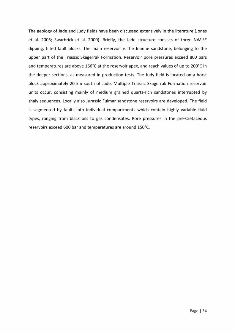
The geology of Jade and Judy fields have been discussed extensively in the literature (Jones

et al. 2005; Swarbrick et al. 2000). Briefly, the Jade structure consists of three NW-SE

dipping, tilted fault blocks. The main reservoir is the Joanne sandstone, belonging to the

upper part of the Triassic Skagerrak Formation. Reservoir pore pressures exceed 800 bars

and temperatures are above 166°C at the reservoir apex, and reach values of up to 200°C in

the deeper sections, as measured in production tests. The Judy field is located on a horst

block approximately 20 km south of Jade. Multiple Triassic Skagerrak Formation reservoir

units occur, consisting mainly of medium grained quartz-rich sandstones interrupted by

shaly sequences. Locally also Jurassic Fulmar sandstone reservoirs are developed. The field

is segmented by faults into individual compartments which contain highly variable fluid

types, ranging from black oils to gas condensates. Pore pressures in the pre-Cretaceous

reservoirs exceed 600 bar and temperatures are around 150°C.

Page | 35

4.1 THE JUDY FIELD

The Judy field located in Block 30/7a in Quadrant 30 of the UK North Sea, 175 miles east-southeast of Aberdeen. In 1985 hydrocarbons were discovered by the 30/7a-4a well on the Judy Field. Excellent flow rates were obtained from both the Pre-Cretaceous Jurassic and Triassic sands. These sands along with the Joanne formations were subsequently appraised by seven more wells drilled between 1985 and 1992, revealing the Judy Pre-Cretaceous reservoir as a complex fault compartmentalized structure.

Figure 5. Judy field area (Offshore technology.com 2012).

Page | 36

4.2 THE JADE FIELD

The Jade Field is an example of a high pressure high temperature heterogeneous fluvial reservoir which, at the time of development, appeared to be a straight-forward case of production by natural depletion. The Jade Field is a high pressure/high temperature (HPHT) gas/condensate field located in the East Central Graben of the North Sea in UKCS Licence Block 30/2c, 270km east of Aberdeen (Figure 6). The field is operated by ConocoPhillips (32.5%) and the remaining ownership consists of BG (35%), Chevron (19.93%), Eni (7%) and OMV (5.57%). The field was discovered in 1996 by well 30/2c-3 and appraised in 1997 by well 30/2c-4. First production was achieved in 2002 through a normally unmanned production wellhead platform connected to the Judy processing facilities in Block 30/7a by a 17km pipeline (Jones et al. 2005).

Figure 6. Location of Jade field and its surrounding fields (Charles 2010).

Page | 37

4.3 PORE PRESSURE PREDICTION BASED ON POROSITY MODEL:

4.3.1 Judy field:

Figure 7. Judy field porosity percentage (Nguyen 2013).

This figure gives the data of porosity (%) along with depth (mbsf). For better understanding

and convenience of calculations, change the units of porosity (fractions) and depth (ft mbsf).

DEPTH (mbsf) POROSITY (%) DEPTH (ftbsf) POROSITY (fraction)

3370 31.5 11056.4 0.135

3440 30.2 11286.0 0.302

3500 27.8 11482.9 0.278

3660 26.6 12007.8 0.266

3730 25.3 12237.5 0.253

3810 23.9 12500.0 0.239

3860 21.4 12664.0 0.214

3980 20.4 13057.7 0.204

4010 17.0 13156.1 0.170

4110 16.8 13484.2 0.168

4220 17.5 13845.1 0.175

4250 13.7 13943.5 0.137

Table 1. Judy field depth-porosity data.

Page | 38

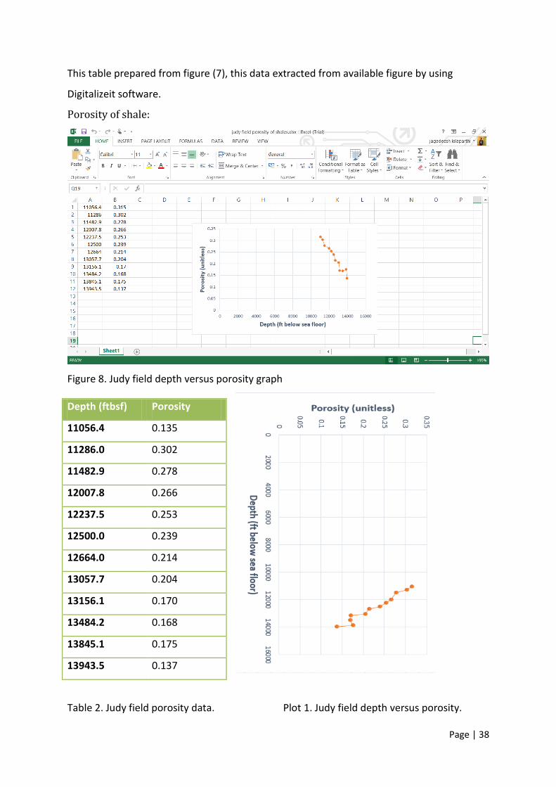
This table prepared from figure (7), this data extracted from available figure by using

Digitalizeit software.

Porosity of shale:

Figure 8. Judy field depth versus porosity graph

Table 2. Judy field porosity data. Plot 1. Judy field depth versus porosity.

Depth (ftbsf) Porosity

11056.4 0.135

11286.0 0.302

11482.9 0.278

12007.8 0.266

12237.5 0.253

12500.0 0.239

12664.0 0.214

13057.7 0.204

13156.1 0.170

13484.2 0.168

13845.1 0.175

13943.5 0.137

Page | 39

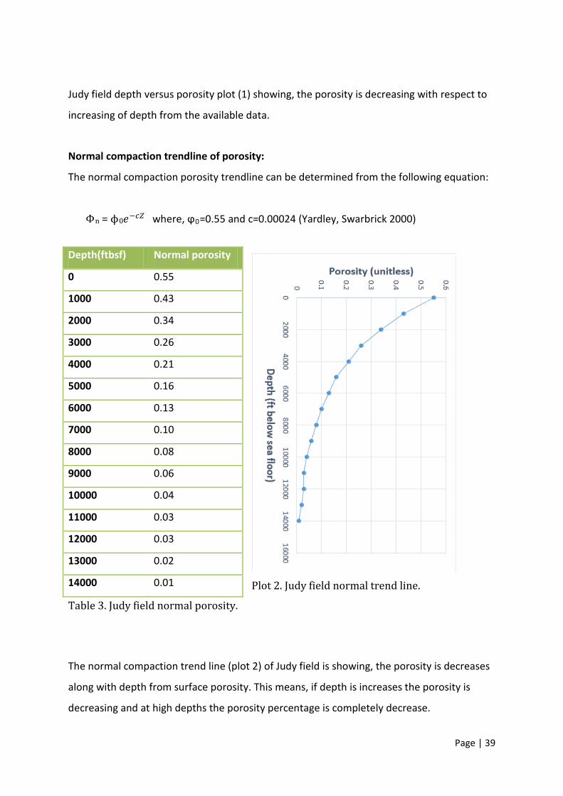
Judy field depth versus porosity plot (1) showing, the porosity is decreasing with respect to

increasing of depth from the available data.

Normal compaction trendline of porosity:

The normal compaction porosity trendline can be determined from the following equation:

Φn = ϕ0𝑒−𝑐𝑍 where, ϕ0=0.55 and c=0.00024 (Yardley, Swarbrick 2000)

Plot 2. Judy field normal trend line.

Table 3. Judy field normal porosity.

The normal compaction trend line (plot 2) of Judy field is showing, the porosity is decreases

along with depth from surface porosity. This means, if depth is increases the porosity is

decreasing and at high depths the porosity percentage is completely decrease.

Depth(ftbsf) Normal porosity

0 0.55

1000 0.43

2000 0.34

3000 0.26

4000 0.21

5000 0.16

6000 0.13

7000 0.10

8000 0.08

9000 0.06

10000 0.04

11000 0.03

12000 0.03

13000 0.02

14000 0.01

Page | 40

Pore pressure gradients:

The pore pressure gradient can be calculated from the following equation:

Ppg = 𝑂𝐵𝐺 − (𝑂𝐵𝐺 − 𝑃𝑛𝑔) 𝑙𝑛𝜙0−𝑙𝑛𝜙𝑐𝑍

where, 𝑃𝑛𝑔= 0.434psi/ft, 𝑂𝐵𝐺= 1psi/ft (Daniel 2000)

Table 4. Judy field pore pressure

gradient.

Plot 3. Judy field pore pressure gradient trend line.

Pore pressure prediction from porosity model gave the result for Judy field, the pore

pressure gradient values (plot 3) are decreasing with respect to depth. However, the

fundamental theory (figure 2) explained, the pore pressure gradient trend line increases

with depth. Thus, the porosity based pore pressure prediction model gave incorrect result

for Judy field.

Depth (ftbsf) Pore pressure

gradient

(psi/ft)

11056.4 0.881

11286.0 0.874

11482.9 0.859

12007.8 0.857

12237.5 0.850

12500.0 0.842

12664.0 0.824

13057.7 0.820

13156.1 0.789

13484.2 0.792

13845.1 0.804

13943.5 0.764

Page | 41

4.3.2 JADE FIELD:

Porosity based pore pressure prediction model verification on Jade field.

Figure 9. Jade field porosity percentage (Nguyen 2013).

Extracted data of depth (mbsf) and porosity (%) convert in terms of depth (ftbsf) and

porosity (fraction).

Depth (mbsf) Porosity (%) Depth (ftbsf) Porosity (fraction)

4390 28.5 14402.8 0.285

4470 27.0 14665.3 0.270

4560 26.4 14960.6 0.264

4660 24.3 15288.7 0.243

4760 22.1 15616.7 0.221

4870 19.9 15977.6 0.199

4910 18.9 16108.9 0.189

4970 18.2 16305.7 0.182

5080 15.9 16666.6 0.159

5130 14.6 16830.7 0.146

5220 12.5 17125.9 0.125

5260 11.0 17257.2 0.110

Table 5. Jade field depth-porosity data.

Page | 42

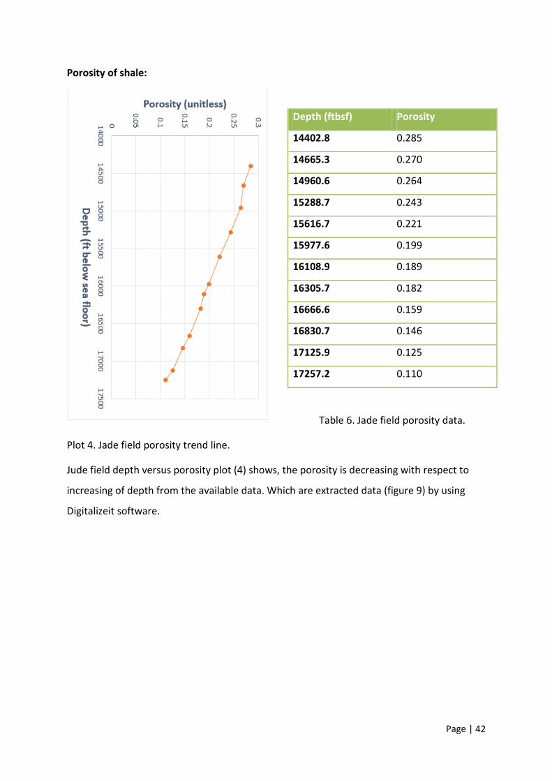
Porosity of shale:

Table 6. Jade field porosity data.

Plot 4. Jade field porosity trend line.

Jude field depth versus porosity plot (4) shows, the porosity is decreasing with respect to

increasing of depth from the available data. Which are extracted data (figure 9) by using

Digitalizeit software.

Depth (ftbsf) Porosity

14402.8 0.285

14665.3 0.270

14960.6 0.264

15288.7 0.243

15616.7 0.221

15977.6 0.199

16108.9 0.189

16305.7 0.182

16666.6 0.159

16830.7 0.146

17125.9 0.125

17257.2 0.110

Page | 43

Normal compaction trendline of porosity:

The normal compaction porosity trendline can be determined from the following equation:

Φn = ϕ0𝑒−𝑐𝑍 where, ϕ0=0.425 and c=0.00024 (Yardley, Swarbrick 2000)

Plot 5. Jade field normal porosity trend line.

Table 7. Jade field normal porosity.

The normal compaction trend line (plot 5) of Jude field is showing, the porosity is decreases

along with depth from surface porosity. This means, if depth is increases the porosity is

decreasing and at high depths the porosity percentage is completely decreased.

Depth (ftbsf) Normal porosity

0 0.425

1000 0.334

2000 0.262

3000 0.206

4000 0.162

5000 0.128

6000 0.100

7000 0.079

8000 0.062

9000 0.049

10000 0.038

11000 0.030

12000 0.023

13000 0.018

14000 0.014

15000 0.011

16000 0.009

17000 0.007

18000 0.005

Page | 44

Pore pressure gradients:

The pore pressure gradient can be calculated from the following equation:

Ppg = 𝑂𝐵𝐺 − (𝑂𝐵𝐺 − 𝑃𝑛𝑔) 𝑙𝑛𝜙0−𝑙𝑛𝜙𝑐𝑍

Where, 𝑃𝑛𝑔= 0.434psi/ft, 𝑂𝐵𝐺= 1psi/ft (Daniel 2000)

Table 8. Jade field pore pressure gradient. Plot 6. Jade field pore pressure gradient trend line

Pore pressure prediction from porosity model gave the result for Judy field, the pore

pressure gradient values (plot 6) are decreasing with respect to depth. However, the

fundamental theory (figure 2) explained, the pore pressure gradient trend line increases

with depth. Thus, the porosity based pore pressure prediction model gave incorrect result

for Jude field.

Depth (ftbsf) Pore pressure

gradient (psi/ft)

14402.8 0.934

14665.3 0.927

14960.6 0.924

15288.7 0.913

15616.7 0.901

15977.6 0.888

16108.9 0.881

16305.7 0.857

16666.6 0.848

17125.9 0.831

17257.2 0.815

Page | 45

4.4 ANALYSIS OF TAU MODEL:

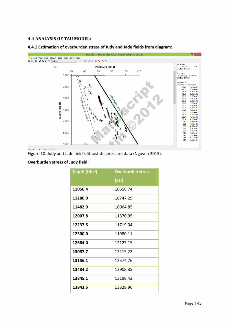
4.4.1 Estimation of overburden stress of Judy and Jade fields from diagram:

Figure 10. Judy and Jade field’s lithostatic pressure data (Nguyen 2013).

Overburden stress of Judy field:

Depth (ftbsf) Overburden stress

(psi)

11056.4 10558.74

11286.0 10747.29

11482.9 10964.85

12007.8 11370.95

12237.5 11719.04

12500.0 11980.11

12664.0 12125.15

13057.7 12415.22

13156.1 12574.76

13484.2 12908.35

13845.1 13198.43

13943.5 13328.96

Page | 46

Table 9. Judy field overburden pressure data.

Judy field overburden (lithostatic) pressure data generated by using the Digitalizeit software

from figure 10. This data (table 10) shows, the overburden pressure is increased along with

depth.

Overburden stress of Jade field:

Table 10. Jade field overburden pressure data. Jude field overburden (lithostatic) pressure data generated by using the Digitalizeit software

from figure 10. This data (table 11) shows, the overburden pressure is increased along with

depth.

Depth (ftbsf) Overburden stress

(psi)

14402.8 13764.07

14665.3 13981.63

14960.6 14271.70

15288.7 14648.80

15616.7 14938.88

15977.6 15228.95

16108.9 15373.99

16305.7 15519.03

16666.6 15954.14

17125.9 16389.26

17257.2 16534.29

Page | 47

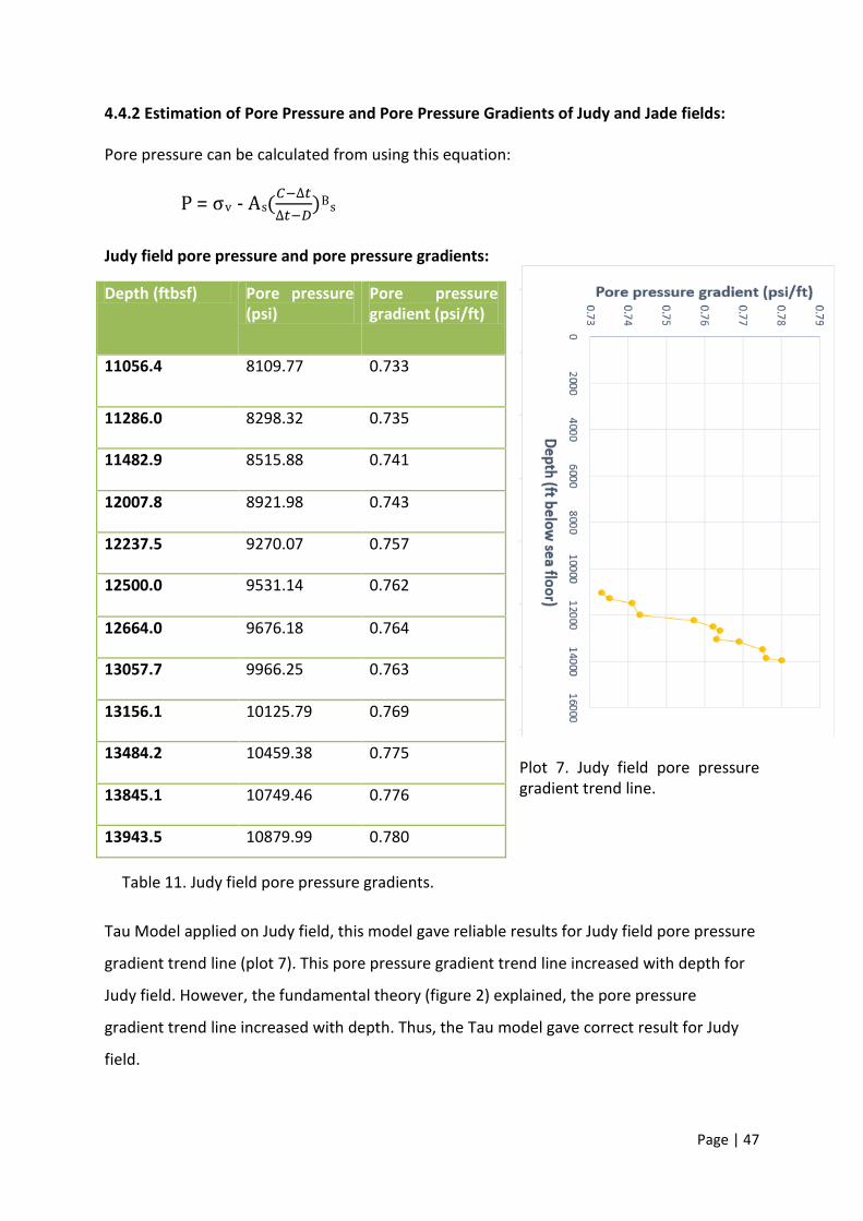
4.4.2 Estimation of Pore Pressure and Pore Pressure Gradients of Judy and Jade fields: Pore pressure can be calculated from using this equation:

P = σv - As(𝐶−∆𝑡∆𝑡−𝐷)P

Bs Judy field pore pressure and pore pressure gradients:

Plot 7. Judy field pore pressure gradient trend line.

Table 11. Judy field pore pressure gradients.

Tau Model applied on Judy field, this model gave reliable results for Judy field pore pressure

gradient trend line (plot 7). This pore pressure gradient trend line increased with depth for

Judy field. However, the fundamental theory (figure 2) explained, the pore pressure

gradient trend line increased with depth. Thus, the Tau model gave correct result for Judy

field.

Depth (ftbsf) Pore pressure (psi)

Pore pressure gradient (psi/ft)

11056.4 8109.77 0.733

11286.0 8298.32 0.735

11482.9 8515.88 0.741

12007.8 8921.98 0.743

12237.5 9270.07 0.757

12500.0 9531.14 0.762

12664.0 9676.18 0.764

13057.7 9966.25 0.763

13156.1 10125.79 0.769

13484.2 10459.38 0.775

13845.1 10749.46 0.776

13943.5 10879.99 0.780

Page | 48

Jade field pore pressure and pore pressure gradients:

Depth (ftbsf) Pore pressure (psi)

Pore pressure gradients (psi/ft)

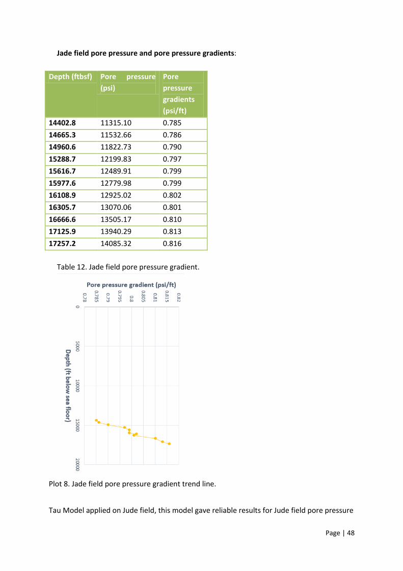
14402.8 11315.10 0.785 14665.3 11532.66 0.786 14960.6 11822.73 0.790 15288.7 12199.83 0.797 15616.7 12489.91 0.799 15977.6 12779.98 0.799 16108.9 12925.02 0.802 16305.7 13070.06 0.801 16666.6 13505.17 0.810 17125.9 13940.29 0.813 17257.2 14085.32 0.816

Table 12. Jade field pore pressure gradient.

Plot 8. Jade field pore pressure gradient trend line.

Tau Model applied on Jude field, this model gave reliable results for Jude field pore pressure

Page | 49

gradient trend line (plot 8). This pore pressure gradient trend line increased with depth for

Jade field. However, the fundamental theory (figure 2) explained, the pore pressure

gradient trend line increased with depth. Thus, the Tau model gave correct result for Jade

field.

4.5 ANALYSIS OF AVAILABLE DATA Pore pressure gradients from available data of Judy and Jade fields:

Figure 11. Judy and Jade fields pore pressure data (Nguyen 2013).

Page | 50

4.5.1 Pore pressure gradients for Judy field: From above diagram depths and pressures converted to feet and psi successively. Depth (ft below sea floor) Pore pressure (psi) Pore pressure gradient (psi/ft) 11056 5612.958 0.507 11286.0 5888.530 0.521 11482.9 6048.072 0.526 12007.8 6555.704 0.545 12237.5 6744.253 0.551 12500.0 7048.832 0.563 12664.0 7585.471 0.598 13057.7 8093.103 0.619 13156.1 8281.652 0.629 13484.2 8658.750 0.642 13845.1 8977.833 0.648 13943.5 9224.397 0.661 Table 13. Judy field pore pressure gradient.

Plot 9. Judy field pore pressure gradient trend line.

Page | 51

Judy field’s pore pressure gradient trendline (plot 9) showed, the pore pressure gradient values increased with respect to depth. This pore pressure gradient data for Judy field generated from figure 10, by using Digitalizeit software. 4.5.2 Pore pressure gradients for Jade field: Depth (ft below sea floor) Pore pressure (psi) Pore pressure gradient

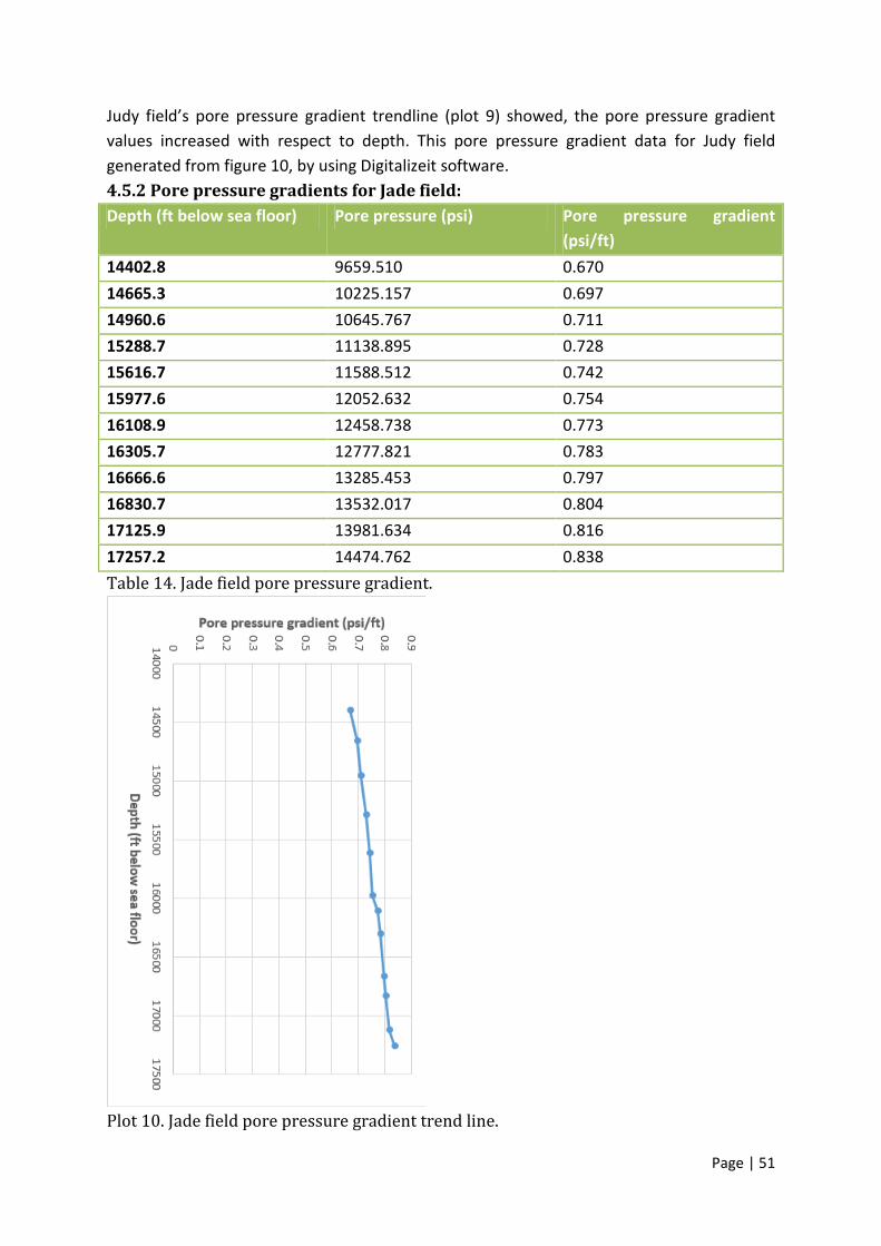
(psi/ft) 14402.8 9659.510 0.670 14665.3 10225.157 0.697 14960.6 10645.767 0.711 15288.7 11138.895 0.728 15616.7 11588.512 0.742 15977.6 12052.632 0.754 16108.9 12458.738 0.773 16305.7 12777.821 0.783 16666.6 13285.453 0.797 16830.7 13532.017 0.804 17125.9 13981.634 0.816 17257.2 14474.762 0.838 Table 14. Jade field pore pressure gradient.

Plot 10. Jade field pore pressure gradient trend line.

Page | 52

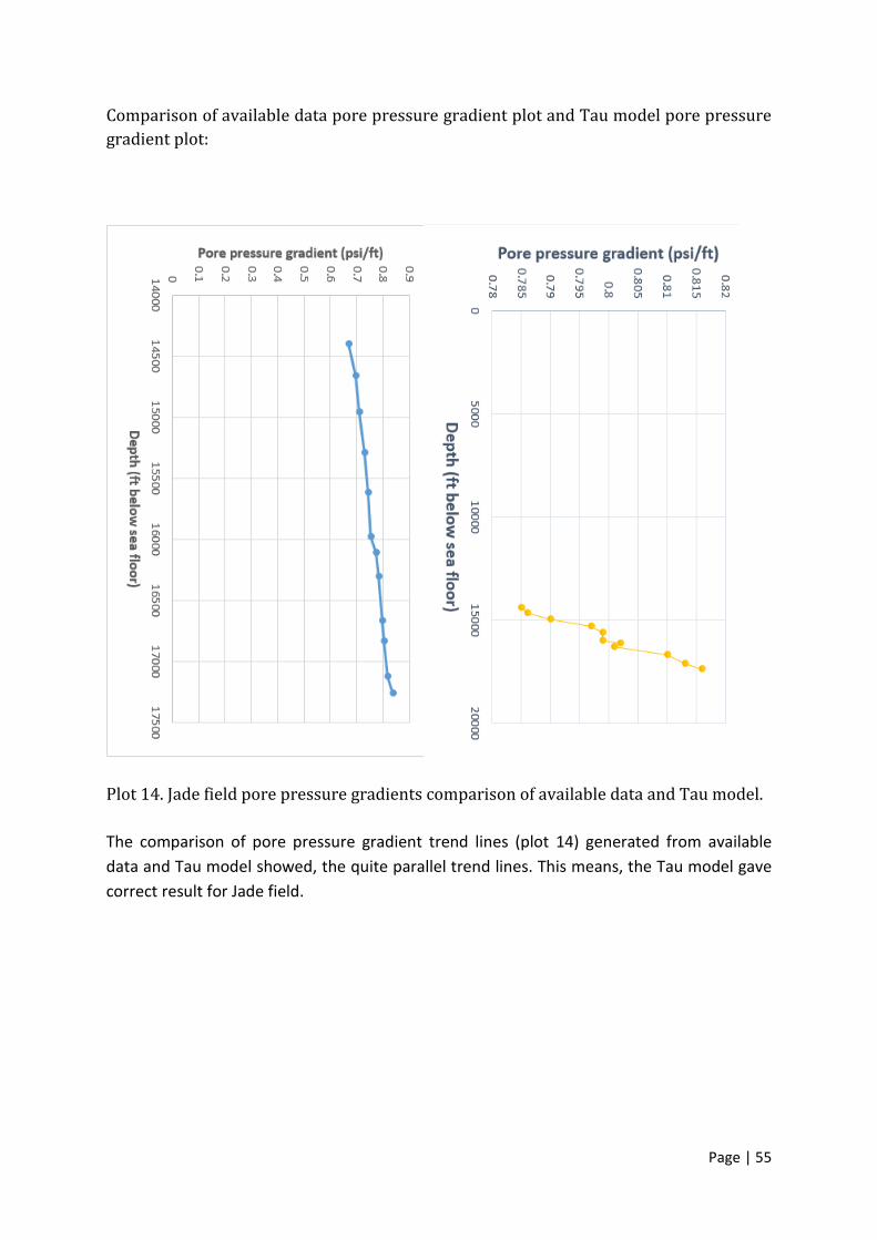
Jade field’s pore pressure gradient trendline (plot 10) showed, the pore pressure gradient values increased with respect to depth. This pore pressure gradient data for Jade field generated from figure 10, by using Digitalizeit software. 4.6 COMPARISON OF PORE PRESSURE GRADIENT RESULTS 4.6.1 Comparison of pore pressure gradient plots for Judy field: Comparison of available data pore pressure gradient plot and porosity based pore pressure prediction model plot:

Plot 11. Judy field pore pressure gradients comparison of available data and porosity based pore pressure prediction model. The comparison of pore pressure gradient trend lines (plot 11) generated from available data and pore pressure prediction from porosity model showed, the quite opposite trend lines. This means, the pore pressure prediction from porosity model gave incorrect result for Judy field.

Page | 53

Comparison of available data pore pressure gradient plot and Tau model pore pressure gradient plot:

Plot 12. Judy field pore pressure gradients comparison of available data and Tau model. The comparison of pore pressure gradient trend lines (plot 12) generated from available data and Tau model showed, the quite parallel trend lines. This means, the Tau model gave correct result for Judy field.

Page | 54

4.6.2 Comparison of pore pressure gradient plots for Jade field: Comparison of available data pore pressure gradient plot and porosity based pore pressure prediction model plot:

Plot 13. Jade field pore pressure gradients comparison of available data and porosity based pore pressure prediction model. The comparison of pore pressure gradient trend lines (plot 13) generated from available data and pore pressure prediction from porosity model showed, the quite opposite trend lines. This means, the pore pressure prediction from porosity model gave incorrect result for Jade field.

Page | 55

Comparison of available data pore pressure gradient plot and Tau model pore pressure gradient plot:

Plot 14. Jade field pore pressure gradients comparison of available data and Tau model. The comparison of pore pressure gradient trend lines (plot 14) generated from available data and Tau model showed, the quite parallel trend lines. This means, the Tau model gave correct result for Jade field.

Page | 56

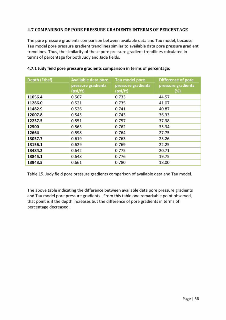
4.7 COMPARISON OF PORE PRESSURE GRADIENTS INTERMS OF PERCENTAGE The pore pressure gradients comparison between available data and Tau model, because Tau model pore pressure gradient trendlines similar to available data pore pressure gradient trendlines. Thus, the similarity of these pore pressure gradient trendlines calculated in terms of percentage for both Judy and Jade fields. 4.7.1 Judy field pore pressure gradients comparison in terms of percentage: Depth (Ftbsf) Available data pore

pressure gradients (psi/ft)

Tau model pore pressure gradients (psi/ft)

Difference of pore pressure gradients (%)

11056.4 0.507 0.733 44.57 11286.0 0.521 0.735 41.07 11482.9 0.526 0.741 40.87 12007.8 0.545 0.743 36.33 12237.5 0.551 0.757 37.38 12500 0.563 0.762 35.34 12664 0.598 0.764 27.75 13057.7 0.619 0.763 23.26 13156.1 0.629 0.769 22.25 13484.2 0.642 0.775 20.71 13845.1 0.648 0.776 19.75 13943.5 0.661 0.780 18.00 Table 15. Judy field pore pressure gradients comparison of available data and Tau model. The above table indicating the difference between available data pore pressure gradients and Tau model pore pressure gradients. From this table one remarkable point observed, that point is if the depth increases but the difference of pore gradients in terms of percentage decreased.

Page | 57

4.7.2 Jade field pore pressure gradients comparison in terms of percentage: Depth (Ftbsf) Available data pore

pressure gradients (psi/ft)

Tau model pore pressure gradients (psi/ft)

Difference of pore pressure gradients (%)

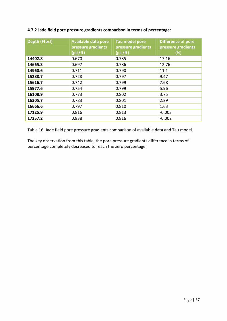
14402.8 0.670 0.785 17.16 14665.3 0.697 0.786 12.76 14960.6 0.711 0.790 11.1 15288.7 0.728 0.797 9.47 15616.7 0.742 0.799 7.68 15977.6 0.754 0.799 5.96 16108.9 0.773 0.802 3.75 16305.7 0.783 0.801 2.29 16666.6 0.797 0.810 1.63 17125.9 0.816 0.813 -0.003 17257.2 0.838 0.816 -0.002 Table 16. Jade field pore pressure gradients comparison of available data and Tau model. The key observation from this table, the pore pressure gradients difference in terms of percentage completely decreased to reach the zero percentage.

Page | 58

4.8 Estimation of Fracture gradients for Judy and Jade fields Finally, chosen Tau model to both Judy and Jade fields, because always pore pressure gradients increase along with depth. By the observation, porosity based pore pressure prediction model failed to satisfy this condition in both Judy and Jade fields. Tau model verified and satisfied the pore pressure gradient conditions on both Jade and Jade fields and addition to that, find the fracture gradients from the Kirsch’s equation (Haimson and Fairhurst, 1970; Zhang and Roegiers, 2010). Tensile failure method (Kirsch’s equation) can be used to find the fracture pressures for both Judy and Jade fields which were verified from Tau model. 𝑃𝐹𝑃 = 3𝑣

2(1−𝑣)(𝜎𝑣 − 𝑝) + 𝑝 𝑣 = 0.3, 0.35 for shale and chalk (Scribd.com 2013)

4.8.1 Fracture gradients for Judy field: Depth (ftbsf) Overburden

stress (psi) Pore pressure (psi) Fracture

gradients (psi/ft)

11056.4 10558.74 8109.77 0.875 11286.0 10747.29 8298.32 0.874 11482.9 10964.85 8515.88 0.878 12237.5 11719.04 9270.07 0.885 12500.0 11980.11 9531.14 0.888 12664.0 12125.15 9676.18 0.888 13057.7 12415.22 9966.25 0.883 13156.1 12574.76 10,125.79 0.889 13484.2 12908.35 10459.38 0.892 13845.1 13198.43 10749.46 0.893 13943.5 13328.96 10879.99 0.893 Table 17. Judy field fracture gradient.

Page | 59

Plot 15. Judy field fracture gradient trend line. Minimum stress method applied on Judy field, this model gave reliable results for Judy field fracture gradient trend line (plot 15). This fracture gradient trend line increased with depth for Judy field. However, the fundamental theory (figure 2) explained, the fracture gradient trend line increased with depth. Thus, the minimum stress method gave correct result for Judy field. 4.8.2 Fracture gradients for Jade field: Depth (ftbsf) Overburden stress

(psi) Pore pressure (psi) Fracture gradients

(psi/ft) 14402.8 13764.07 11315.10 0.922 14665.3 13981.63 11532.66 0.921 14960.6 14271.70 11822.73 0.922 15288.7 14648.80 12199.83 0.927 15616.7 14938.88 12489.91 0.926 15977.6 15228.95 12779.98 0.923 16108.9 15373.99 12925.02 0.925 16305.7 15519.03 13070.06 0.922 16666.6 15954.14 13505.17 0.928 17125.9 16389.26 13940.29 0.929 17257.2 16534.29 14085.32 0.930 Table 18. Jade field fracture gradient.

Plot 16. Jade field fracture gradient trend line.

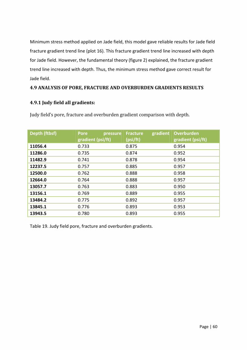
Page | 60

Minimum stress method applied on Jade field, this model gave reliable results for Jade field

fracture gradient trend line (plot 16). This fracture gradient trend line increased with depth

for Jade field. However, the fundamental theory (figure 2) explained, the fracture gradient

trend line increased with depth. Thus, the minimum stress method gave correct result for

Jade field.

4.9 ANALYSIS OF PORE, FRACTURE AND OVERBURDEN GRADIENTS RESULTS

4.9.1 Judy field all gradients: Judy field’s pore, fracture and overburden gradient comparison with depth. Depth (ftbsf) Pore pressure

gradient (psi/ft) Fracture gradient (psi/ft)

Overburden gradient (psi/ft)

11056.4 0.733 0.875 0.954 11286.0 0.735 0.874 0.952 11482.9 0.741 0.878 0.954 12237.5 0.757 0.885 0.957 12500.0 0.762 0.888 0.958 12664.0 0.764 0.888 0.957 13057.7 0.763 0.883 0.950 13156.1 0.769 0.889 0.955 13484.2 0.775 0.892 0.957 13845.1 0.776 0.893 0.953 13943.5 0.780 0.893 0.955 Table 19. Judy field pore, fracture and overburden gradients.

Page | 61

Plot 17: Comparison of pore, fracture and overburden gradients of Judy field. All pressure gradients such as pore pressure gradient, fracture gradient and overburden pressure gradients compared with depth in the plot 17, this trend lines similar to fundamental theory (figure 2) trend lines. Thus, the chosen models gave correct results and verified on Judy field. 4.9.2 Jade field all gradients: Jade field’s pore, fracture and overburden gradient comparison with depth.

Table 20. Jade field pore, fracture and overburden gradients.

Depth (ftbsf) Pore pressure gradient (psi/ft)

Fracture gradient (psi/ft)

Overburden gradient (psi/ft)

14402.8 0.785 0.922 0.955 14665.3 0.786 0.921 0.953 14960.6 0.790 0.922 0.953 15288.7 0.797 0.927 0.958 15616.7 0.799 0.926 0.956 15977.6 0.799 0.923 0.953 16108.9 0.802 0.925 0.954 16305.7 0.801 0.922 0.951 16666.6 0.810 0.928 0.957 17125.9 0.813 0.929 0.956 17257.2 0.816 0.930 0.958

Page | 62

Plot 18: Comparison pore, fracture and overburden gradients of Jade field All pressure gradients such as pore pressure gradient, fracture gradient and overburden pressure gradients compared with depth in the plot 18, this trend lines similar to fundamental theory (figure 2) trend lines. Thus, the chosen models gave correct results and verified on Jade field.

Page | 63

CHAPTER 5 5.0 CONCLUSIONS AND RECOMMENDATIONS 5.1 CONCLUSIONS: The purpose of this project was to develop a pore pressure and fracture gradient prediction strategy for the Judy and Jade fields in the North Sea Central Graben. The offset well data consisted of Judy and Jade HPHT fields. Multiple pore pressure prediction strategies were reviewed that gave reasonable results: Pore pressure prediction from porosity model and Tau model equations for both porosity and seismic velocity data. Attempts were made to verify the validity of these approaches by comparing the results with pressure depth for sediments. Those attempts gave reasonable results in both fields. However, porosity based pore pressure prediction model does not always deliver a satisfactory pore pressure estimation. There were several reasons for failure to the porosity based method, especially in high temperature basins and higher depths. Pore pressure prediction from porosity model, gave the pore pressure gradients for both Judy and Jade fields were fluctuated and decreased along with depth increased. Tau model gave the good results in both fields, those pore pressure gradients increased along with depths increased. The significant point was the Tau model more appropriate at high depths, because from table 15 and table 16, the pore pressure gradients at high depths similar to available pore pressure gradients, thus the Tau model more suitable to predict the pore pressure gradients at higher depths and overpressured fields. This scenario explained and supported the fundamental lithostatic gradient plot. Therefore, the Tau model was concluded to be the best pore pressure prediction method for future wells in Judy and Jade fields. The fracture gradient prediction method proposed by Kirsch’s solution (tensile failure method) was practical using area precise information and an autonomous foundation for the connection between Poisson’s ratio and pore pressure. This method allows fracture gradient prediction and was concluded to be appropriate for future use in these areas.

Page | 64

5.2 RECOMMENDATIONS: While the above-mentioned pore pressure and fracture gradient prediction methods were allowed for the limited availability and quality of data, there was certain improbability in the precision of the forecasts. The following commendations concerning those uncertainties should be addressed when planning and conducting future drilling operations.

• Porosity based pore pressure prediction method can deliver suitable pore pressure prediction where the overpressure is under compaction and the deposits are young and at low temperatures. Identifying the petroleum systems are both complex and varied, and constantly postulate a series of improbability in pore pressure prediction for future wells.

• Calibration using offset wells, emerging local consideration of wireline and rock

characteristics to standardise prediction results. Retaining field modelling seismic and wireline based prediction techniques deliver balancing outcomes and appreciated perceptions into the accurate series of improbability in prediction.

• The best fitting parameters of the Tau model varies from region to region, the

assumed fitting parameters to be depends on region lithology. Realistic pore pressures are required to make reliable fracture gradient calculations.

Page | 65

REFERENCES

Ashton, K., Sylte, J.E., Thomas, L.K., and Dixon, T.N. (1998) ‘Judy/Joanne Field Development.’ [online] available from: < http://www.onepetro.org/mslib/app/Preview.do?paperNumber=00049128&societyCode=SPE> [27-30 Sep. 1998]

Bowers, G.L. (2001) ‘Determining an Appropriate Pore-Pressure Estimation Strategy.’ [online] available from: < http://www.onepetro.org/mslib/servlet/onepetropreview?id=OTC-13042-MS>[30 April-3 May 2001]

Bowers, G.L. (1995) ‘Pore Pressure Estimation from Velocity Data: Accounting for Overpressure Mechanisms besides Undercompaction.’ Journal of SPE Drilling & Completion 10, 89-95

Burrus, J. (1998) ‘Overpressure models for clastic rocks, their relation to hydrocarbon expulsion: a critical reevaluation.’ In: Law, B.E., Ulmishek, G.F., Slavin, V.I. (Eds.), Abnormal pressures in hydrostatic environments: AAPG Memoir, 70, pp.35-63

Chatterjee, A., Mondal, S., Basu, P., Patel, B.K., and Reliance Industries Limited (Petroleum E&P). (2012) ‘Pore Pressure Prediction Using Seismic Velocities for Deepwater High Temperature- High Pressure Well in Offshore Krishna Godavari Basin, India.’ [online] available from: <http://www.onepetro.org/mslib/app/Preview.do?paperNumber=SPE-153764-MS&societyCode=SPE> [28-30 Mar.2012]

Daines, S.R. (1982) ‘Prediction of Fracture Pressures for Wildcat Wells.’ [online] available from: <http://www.onepetro.org/mslib/servlet/onepetropreview?id=00009254>[April 1982]

Daniel, R.B. (2001) ‘Pressure prediction for a Central Graben wildcat well, UK North Sea.’ Marine and Petroleum Geology, 18, 235-250

Dickinson, G. (1951) ‘Geological Aspects of Abnormal Reservoir Pressures in the Gulf Coast Region of Louisiana, U.S.A.’ [online] available from: <http://www.onepetro.org/mslib/servlet/onepetropreview?id=WPC-4001>[May 28 - June 6, 1951]

Dutta, N.C. (2002) ‘Geopressure prediction using seismic data: Current status and the road ahead.’ Geophysics, 67, 2012-2041

Eaton, B.A. (1968) ‘Fracture Gradient Prediction and Its Application in Oilfield Operations.’ Petroleum Technology, 21, 1353-1360

Page | 66

Eaton, B.A. (1972) ‘The Effect of Overburden Stress on Geopressure Prediction from Well Logs.’ Petroleum Technology, 24, 929-934

Eaton, B.A. (1975) ‘The Equation for Geopressure Prediction from Well Logs.’ [online] available from: < http://www.onepetro.org/mslib/servlet/onepetropreview?id=00005544>[ September-1 October 1975]

Flemings, P.B., Stump, B.B., Finkbeiner, T., Zoback, M. (2002) ‘Flow focusing in overpressured sandstones: theory, observations, and applications. Am. J. Sci.302, 827-855

Fooshee, J.S. (2009) ‘The development of a pore pressure and fracture gradient prediction model for the Ewing banks 910 area in THE Gulf of Mexico.’ [online] available from: <http://etd.lsu.edu/docs/available/etd-01202009-143411/> [20 Jan. 2009]

Gardner, G.H.F., Gardner, L.W., Gregory, A.R. (1974) ‘Formation velocity and density-the diagnostic basis for stratigraphic traps.’ Geophysics, 39, 2085-2095

Gutierrez, M.A., Braunsdor, N.R., and Couzens, B.A. (2006) ‘Calibration and ranking of pore-pressure prediction models.’ The Leading Edge, 25, 1516–1523

Haimson, B.C., Fairhurst, C. (1970) ‘In situ stress determination at great depth by means of hydraulic fracturing.’ In: Somerton, W.H. (Ed.), Rock Mechanics-theory and practice. Am. Inst. Mining. Eng., pp. 559-584

Hawkins, K., Ratcliffe, A., Roberts, G., Went, D. and DGC, V. (2004) High Resolution Pore-pressure Prediction from AVO Derived Velocities; a North Sea Case Study [online] available from <http://www.onepetro.org/mslib/servlet/onepetropreview?id=SEG-2004-0366>

Heppard, P.D., Cander, H.S., Eggertson, E.B. (1998) ‘Abnormal pressure and the occurrence of hydrocarbons in offshore eastern Trinidad, West Indies.’ In: Law, B.E., Ulmishek, G.F., Slavin, V.I. (Eds.), Abnormal Pressures in Hydrocarbon Environments: AAPG Memoir, 70, pp. 215-246

Holbrook,P.W., Maggiori, D.A. (1995) ‘Real-Time Pore Pressure and Fracture Gradient Evaluation in All Sedimentary Lithologies.’ SPE Formation Evaluation, 10, 215-222

Hottmann, C.E., Johnson, R.K. (1965) ‘Estimation of Formation Pressures from Log-Derived Shale Properties.’ Petroleum Technology, 17, 717-722

Law, B.E., Spencer, C.W. (1998) ‘Abnormal pressures in hydrocarbon environments.’ In: Law, B.E., Ulmishek, G.F., Slavin, V.I. (Eds.), Abnormal Pressures in Hydrocarbon Environments: AAPG Memoir, 70, pp. 1-11

Morley, C.K., King, R., Hillis, R., Tingay, M., Backe, G. (2011) ‘Deepwater fold and thrust belt classification, tectonics, structure and hydrocarbon prospectivity: A review.’ Earth-Science Review, 104, 41-91

Page | 67

Mouchet, J.C., Mitchell, A. (1989) ‘Abnormal Pressure while Drilling.’ Editions TECHINIP, Paris

Nelson, H.N., Bird, K.J. (2005) ‘Porosity-Depth Trends and Regional Uplift Calculated from Sonic Logs, National Reserves in Alaska.’ Scientific Investigation Report 2005-5051 U.S. Dept. of the Interior and USGS

Nguyen, T.T.B; Jones, J.S; Goulty, N.R; Middleton, A.J; Grant, N; Ferguson, A; Bowen, L. (2013) ‘The role of fluid pressure and diagenetic cements for porosity preservation in Triassic fluvial reservoirs of the Central Graben, North Sea.’ the American Association of Petroleum Geologists, 97, 1273-1302

Nygaard, R., Karimi, M., Hareland, G., Tahmeen, M., and Munro, H. (2008) ‘Pore Pressure Prediction in Overconsolidated Shales.’ [online] available from: < http://www.onepetro.org/mslib/app/Preview.do?paperNumber=SPE-116619-MS&societyCode=SPE>[11-15 Oct. 2008]

Ovens, J., Charles, R. (2010) ‘Jade field: Late - life development challenges in a Triassic HPHT gas condensate reservoir.’ [online] available from : < http://petex.pesgb.org.uk/cgi-bin/somsid.cgi?page=html/abstracts/abstractid49> [18 Aug. 2013]

Offshore technology (2012) ‘Jasmine Field, North Sea, United Kingdom.’ [online] available from: < http://www.offshore-technology.com/projects/jasminefieldnorthsea/> [18 Aug.2013]

Powley, D.E. (1990) ‘Pressures and hydrogeology in petroleum basins.’ Earth-Science Reviews, 29, 215-226

Primio, R. D., Neumann, V. (2008) ‘HPHT reservoir evolution: a case study from Jade and Judy fields, Central Graben, UK North Sea.’ Earth Sciences, 97, 1101-1114

Sborne, M.J., Swarbrick, R.E. (1999) ‘Diagenesis in North Sea HPHT clastic reservoirs — consequences for porosity and overpressure prediction.’ Marine and Petroleum Geology, 16, 337-353

Sayers, C.M., Johnson, G.M., Schlumberger., Denyer, G., and EEX Corporation. (2000) ‘Predrill Pore Pressure Prediction Using Seismic Data.’ [online] available from : < http://www.onepetro.org/mslib/servlet/onepetropreview?id=00059122> [23-25 Feb. 2000]

Swarbrick, R.E., Osborne, M.J., Grunberger, D., Yardley, G.S., Macleod, G., Aplin, A.C., Larter, S.R., Knight. V. and Auld, H.A. (2000) ‘Integrated study of the Judy Field (Block 30/7a) — an overpressured Central North Sea oil/gas field’. Marine and Petroleum Geology, 17, 993–1010

Page | 68

Swarbrick, R.E. (2001) ‘Challenges of porosity – based pore pressure prediction.’ [online] available from: <http://www.earthdoc.org/publication/publicationdetails/?publication=4437>

Swarbrick, R. (2012) ‘Review of pore-pressure prediction challenges in high-temperature areas’. The Society of Exploration Geophysicists, 31, 1288-1294

Swarbrick, R.E., Osborne, M.J. (1998) ‘Mechanisms that generate abnormal pressures: an overview. In: Law, B.E., Ulmishek, G.F., Slavin, V.I. (Eds.), Pressure Regimes in Sedimentary Basins and their Prediction: AAPG Memoir, 70, pp. 13-34

Swarbrick, R.E., Osborne, M.J., Yardley, G.S. (2002) ‘Comparison of overpressure magnitude resulting from the main generating mechanisms. In: Huffman, A.R., Bowers, G.L. (Eds.), Pressure Regimes in Sedimentary Basins and their Prediction: AAPG Memoir, 76, pp. 1-12

Ward, C.D., Sperry-Sun Drilling Services; Coghill, K., BP Norge U.A.; Broussard, M.D., and Amoco Norway Oil Company. (1994) ‘The Application of Petrophysical Data to Improve Pore and Fracture Pressure Determination in North Sea Central Graben HPHT Wells.’ [online] available from:< http://www.onepetro.org/mslib/app/Preview.do?paperNumber=00028297&societyCode=SPE>[25-28 Sep.1994]

Winthaegen, P.L.A., Verweij, J.M. (2003) ‘Estimating regional pore pressure distribution using 3D seismicvelocities in the Dutch Central North Sea Graben.’ Geochemical Exploration, 78-79, 203–207

Yardley, G.S., Swarbrick, R.E. (2000) ‘Lateral transfer: a source of additional overpressure?.’ Marine and Petroleum Geology, 17, 523-537

Zhang, J. (2011) ‘Pore pressure prediction from well logs: Methods, modifications, and new approaches.’ Earth-Science Reviews, 108, 50–63