Computers, Environment and Urban Systems 34 (2010) 400–408

Contents lists available at ScienceDirect

Computers, Environment and Urban Systems

journal homepage: www.elsevier .com/locate /compenvurbsys

The impact of variation in scale on the behavior of a cellular automata usedfor land use change modeling

Ying Pan a, Andreas Roth b, Zhenrong Yu a,*, Reiner Doluschitz b

a College of Resources and Environmental Sciences, China Agricultural University, Beijing 100193, Chinab Computer Applications and Business Management in Agriculture, University of Hohenheim (410C), 70593 Stuttgart, Germany

a r t i c l e i n f o

Article history:Received 6 October 2009Received in revised form 13 March 2010Accepted 13 March 2010

Keywords:Land use changeCellular automata modelScaleNeighborhoodParameterNorth China Plain

0198-9715/$ - see front matter � 2010 Elsevier Ltd. Adoi:10.1016/j.compenvurbsys.2010.03.003

* Corresponding author. Tel.: +86 10 62731293; faxE-mail addresses: alanpan1224@gmail.com (Y. Pa

(A. Roth), yuzhr@cau.edu.cn (Z. Yu), agrarinf@uni-hoh

a b s t r a c t

The cellular automata (CA) model is an important tool in land use studies. Scale is a central concept inboth land use research and CA models. To better understand the connection between different scalesand processes of land use change, more studies on the behavior of a CA model at different scales are nec-essary and urgent. The objective of this study was to explore the impact of variation in scale on thebehavior of a CA employed for land use change modeling. The scale variation was represented by the var-iation in the spatial extent of the images used, in the cell size and in the neighborhood configuration,including the size and shape. Two aspects of the behavior of the model were examined: the algorithmsexpressing the land use transitions, and the precision of the model’s output. The average enrichment fac-tor, which generates the transition rules, was used to quantify the interpretation of the land use transi-tions. The kappa index was used to quantify the precision of the model’s output. The results showed thatthe variation of the spatial extent, cell size, and neighborhood size and shape influenced the model’sbehavior in different ways. A combination of small cell size and small neighborhood size generatedimproper expressions of the land use transitions. Here, we believe that an increase in the neighborhoodsize might be the solution. However, the precision of the simulation decreased when the neighborhoodsize increased with ring shape. In addition, the precision first increased and then decreased once theneighborhood size reached a certain value for a scope-shaped neighborhood. Based on these results,we recommend the finest resolution and a neighborhood size of 9 � 9 cells arranged in a scope shape.This set of parameters reflects the most accurate land information. The model interprets well the landuse transitions that are identical to those found in actual ‘‘real” land transitions and also provideshigh-precision outputs. For different model applications at different spatial scales, a preliminary discus-sion of the scale parameter setting is recommended.

� 2010 Elsevier Ltd. All rights reserved.

1. Introduction

1.1. Background

Land use activities have transformed a large proportion of theplanet’s land surface, mainly for agronomic reasons, seeking tosatisfy increasing human needs at the expense of environmentalconditions (Foley et al., 2005). Many projects have focused on landuse and cover change (LUCC) since the end of the last century(Lambin et al., 1999; Turner et al., 1995). The key issues outlinedby the LUCC agenda include the study of integrated global andregional models and the development of databases on landsurfaces, biophysical process and their drivers (Lambin et al.,1999).

ll rights reserved.

: +86 10 6273 2430.n), a.roth@uni-hohenheim.deenheim.de (R. Doluschitz).

The cellular automata (CA) model is frequently used in land sur-face studies. The cell representation of CA is similar in its spatialcharacteristics to remote sensing images and raster GIS, which of-ten provide the land surface data (Ménard & Marceau, 2005). TheCA model also provides explicit handling of dynamic spatial mod-els with time (Wagner, 1997). The background of a CA is in the sim-ulation of processes of neighboring interacting cells. This approachis similar to land use activities, which are often characterized bythe interaction of neighboring landscape patterns. Several exam-ples of land use change based on neighborhood interaction arefound in the literature, such as (1) urbanization due to the neigh-boring road network attraction (Clarke, Hoppen, & Gaydos, 1997),(2) growth of existing residential centers due to centripetal forces(Verburg, van Eck, de Nijs, Visser, & de Jong, 2004) and (3) defores-tation due to new residential development (Schneider & Pontius,2001). The land use transition being modeled is entirely encapsu-lated in the transition rules, allowing a link between the patternsand the underlying process (Ménard & Marceau, 2005).

Y. Pan et al. / Computers, Environment and Urban Systems 34 (2010) 400–408 401

1.2. Scale issue in land use modeling

Scale is a central concept in describing and explaining the com-plex hierarchical organization of the geographic world (Marceau,1999). Many environmental problems connected with land usechange cannot be handled at one single scale of observation, suchas environmental degradation due to agricultural activities, waterresource management, timber extraction and deforestation, globalwarming and air quality, and infectious diseases (Foley et al.,2005). An understanding of how processes operate at various spa-tial scales and how they can be linked across scales is thus a primarygoal in investigating these complex phenomena (Marceau, 1999).

In a CA, scale is defined by three components: the spatial extent,the cell size, and the neighborhood configuration (Ménard & Mar-ceau, 2005). The extent is the total length, area or volume that existsor is observed or analyzed (Dungan et al., 2002). In a CA, the extentrefers to the dimension of the area that is modeled (Ménard & Mar-ceau, 2005). The cell size is the actual area of the landscape each cellwill cover. Most CA models possess a homogeneous cell space. Eachcell has either one or a set of values to represent aspects that charac-terize the land surface, such as land use type, land use degree state orsoil quality. Neighborhood configuration determines the distribu-tion and number of neighbors that will have an impact on the evolu-tion of each cell (Ménard & Marceau, 2005). Neighborhoodconfiguration in a CA is generally characterized by neighborhoodshape, size and/or distance (radius) (Barredo & Demicheli, 2003;Kocabas & Dragicevic, 2006; Ménard & Marceau, 2005; Samat, 2006).

The scale decisions involved in the application of a CA oftendepend on the region and data availability. Ménard and Marceau(2005) concluded, from the scale decisions in 17 different studiescovering nearly 10 years, that the applicable cell size ranged fromless than 50 m to 1 km. The spatial extent of the 17 studies rangedfrom the watershed level to an entire country, and the neighbor-hood configurations also differed. Many scientists have argued thatCA models are sensitive to variations in scale (Kocabas & Dragic-evic, 2006; Ménard & Marceau, 2005; Samat, 2006).

Pontius and Neeti (2010) grouped the sources of the sensitivityand uncertainty under three headings: data, model and future landuse change processes. Future land use change processes can beuncertain because decision making involves human free will(Pontius & Neeti, 2010). The other two headings, the data and mod-el, can be uncertain due to scale variations among different studies.First, data rasterization and aggregation are often used on thevector data and the original remote sensing images to producethe model input data. Dendoncker, Schmit, and Rounsevell (2008)evaluated errors and uncertainties in representing landscapes thatarise from different data rasterization methods and spatial resolu-tions. The results showed that, for example, the use of the pointmethod of rasterization created more fragmented landscapes,while the majority method of rasterization underestimated minorLU classes; this underestimation effect increased with the cell size(Dendoncker et al., 2008). These uncertainties in the input datathat arise from data aggregation will influence the precision ofthe model output. To reduce the uncertainties, fine resolutionmaps seem to be a better choice, but they can also increase thecomputational demand.

Models contain various types of uncertainty, associated withhow accurately their algorithms express important processes anduse those relationships to simulate land use transitions (Pontius &Neeti, 2010). These relationships, expressed with algorithms forland use transitions, are affected by scale variations, including cellsize and neighborhood configurations. Ménard and Marceau(2005) explored the spatial scale sensitivity of a CA model for landuse modeling. Four resolutions and six different neighborhood con-figurations were considered. The results showed that the spatialscale had a considerable impact on the simulation results, including

the land cover area and the spatial structure. As regards the level ofdetail, the simulations with a small cell size generated more than 30times the number of patches present in the original map, whereasother larger cell sizes remained relatively close to the original. Vari-ations in the cell size contributed more uncertainties to the simula-tion results than those in the neighborhood configuration. Samat(2006) characterized the scale sensitivity of the CA model simulat-ing urban growth. The results showed that the model performance,including the precision tested by kappa indices and the modeled ur-ban morphology tested by shape index, will be influenced by thecell size variation, and the model performance is better at the smallcell size. Kocabas and Dragicevic (2006) assessed CA model behav-ior using a sensitivity analysis approach. The results showed that inaddition to the cell size, the neighborhood size and type configura-tions also had a significant influence on the CA model output. Dif-ferent sizes and types of neighborhoods will generate differentsimulated patterns and different numbers of patches.

1.3. Evaluation on scale effects

There are several methods to evaluate the impact of scale varia-tion on the model performance. These methods include using a kap-pa index and an extended kappa index to evaluate the quantificationand location errors in a comparison between two cellular maps(Pontius, 2000). Another method of evaluation is to use the percent-age of landscape agreement or disagreement to compare the predic-tive map with the null model at multiple resolutions (Pontius,Huffaker, & Denman, 2004). Comparisons can also be made betweenthe reference map of the initial time and the reference map of asubsequent time along with the prediction map for the subsequenttime in order to evaluate the model (Pontius & Neeti, 2010; Pontiuset al., 2008). Sensitivity analysis can also be applied, by evaluatingthe effect of changing one variable or a combination of factors onthe overall performance of the model (Kocabas & Dragicevic,2006; Ménard & Marceau, 2005; Samat, 2006). The value of theevaluation is in the quantificational comparison. The percent oflandscape or area in agreement and disagreement, along with thekappa index, which focuses on the pixel-by-pixel analysis, and thelandscape metrics, which focus on the pattern-by-pattern analysis,are the most commonly used quantificational indices.

1.4. Our objective

The objective of this study was to evaluate the impact of varia-tion in scale on the behavior of the CA model. The scale variationwas represented by the variation of spatial extent, cell size andneighborhood configuration including shape and size. The impactof variations in cell size on the model precision has been discussedin many studies (Ménard & Marceau, 2005; Samat, 2006), as hasthe neighborhood configuration variation (Kocabas & Dragicevic,2006). Our aim was to study the impact of scale on the overallmodel behavior. First, we evaluated the response of the algorithmexpression of important land use transitions to the scale variationincluding spatial extent, cell size, neighborhood shape and size.Second, we evaluated the impact of scale variation on the modelprecision by comparing the reference map and the predictionmap for the identical time period. The scale variation in the secondapproach focused more on the neighborhood shape and size.

2. Data and methods

2.1. The CA model – CLUE-S

The model used in this study, CLUE-S (The Conversion of LandUse and its Effects), was developed by the CLUE group (Veldkamp

Fig. 1. Characterization of neighborhood. (a) Ring shape neighborhood with a size of 3 � 3 cells. (b) Ring shape neighborhood with a size of 5 � 5 cells. (c) Scope shapeneighborhood with a size of 3 � 3 cells. (d) Scope shape neighborhood with a size of 5 � 5 cells (modified from Fonstad (2006)).

402 Y. Pan et al. / Computers, Environment and Urban Systems 34 (2010) 400–408

& Fresco, 1996; Verburg, de Koning, Kok, Veldkamp, & Bouma,1999; Verburg et al., 2002; Verburg, Eickhout, & van Meijl, 2008).CLUE-S is a grid-based, multi-scale, spatially-explicit and dynamicsimulation model. It is used to analyze land use patterns and tosimulate near-future changes. The original CLUE-S model is basedon empirical characterizations of location suitability for typicalland use types. Verburg et al. (2004) introduced a simple methodfor exploring and quantifying the neighborhood characteristics ofland use patterns and discussed the ability to assist the definitionof transition rules for CA models. Duan, Verburg, Zhang, and Yu(2004) introduced this method to the CLUE-S model and simulatedthe urban expansion of the Haidian district of Beijing City in China.In that approach, the transition rules were generated as functionsof the neighborhood interactions combined with land suitability,such as accessibility and slope (Verburg et al., 2002). In this paper,the transition rules were generated as the function of neighbor-hood interactions only.

2.2. Characterization of a model neighborhood

A neighborhood is any set of one or more locations that arewithin a specified distance and/or have a directional relationshipto a particular location (Tomlin, 1990; in Verburg, de Nijs, vanEck, Visser, & de Jong (2004)). In this study, the ‘specified distance’is characterized by the definition of a neighborhood shape and size(Fig. 1). The directional relationship is identified by the neighbor-hood interaction algorithm (Eq. (1)).

The neighborhood shapes assumed in this study are scope andring shapes. The scope shape is identical to both the Moore neigh-borhood and the extended Moore neighborhood (Fonstad, 2006),which is defined as a square-shaped neighborhood. The central cellof the square is the simulated core cell defined by its neighbor-hood. The ring neighborhood shape is characterized by the outer-most circle cells within a defined distance, similar to the scopeneighborhood. The size of a neighborhood is equal to the numberof cells of one side row/column. The smallest neighborhood sizein our study was a rectangle of three columns by three row cells(3 � 3). The enlarged neighborhood sizes, in turn, should be5 � 5, 7 � 7, 9 � 9, 11 � 11, 13 � 13, 15 � 15, and so on.

2.3. The transition rules used

The transition rules are the core variables of a CA model, repre-senting the logarithmic expression of the land use transitions beingmodeled. These rules effectively determine the dynamic spatial re-sults of a CA approach (White & Engelen, 2000).

In this research, the transition rules of the CLUE-S model werecalculated based on neighborhood interactions. These interactionsare generated based on the layout of land use patterns at one spe-cific time. Verburg et al. (2004) introduced a method to calculate

the interactions based on land use patterns. The enrichment factor(F) defines the abundance of a land use type in the neighborhood ofthe central cell. This factor is determined in relation to the occur-rence of the land use type in the entire landscape as follows (Eq.(1)) (Verburg, de Nijs et al., 2004):

Fi;k;d ¼nk;d;i=nd;i

Nk=N; ð1Þ

where i is the cell location, k is the land use type, d is the neighbor-hood size, Fi,k,d is the relative enrichment of the land use type kwithin a size d in the neighborhood of the cell in location i, nk,d,I

is the grid amount of land use type k in the neighborhoods d of celli, nd,i is the total amount of cells in the neighborhood with size d, Nk

is the amount of cells of land use type k in the whole landscape, N isthe total number of cells.

The interaction between different land use types is determinedwith the average enrichment factor derived from Fi,k,d as follows(Eq. (2)):

�Fl;k;d ¼1Nl

X

i2L

Fi;k;d; ð2Þ

where �Fl;k;d is the interaction between land use type k and l, Nl is thetotal grid amount that is equal to land use type l, L is the set of allgrids of land use type l, �Fl;k;d is a positive floating number.

The average enrichment factor is a positive value with0 < �Fl;k;d < 1, which means that the two land types are repulsive,and 1 < �Fl;k;d < +1 indicates the opposite attractive effects. To nor-malize the positive or negative value of �Fl;k;d; the log (�Fl;k;d) was usedin our study to evaluate the neighborhood interaction. If the valueof log (�Fl;k;d) calculated from one twin-counteracting land type isnegative, then the interaction between the two land types at thelandscape level is repulsive. The repulsive effect becomes weakeras the value nears zero. If log ð�Fl;k;dÞ ¼ 0, then the interaction is nei-ther attractive nor repulsive. If the value of log (�Fl;k;d) is positive,then the interaction is attractive, and the attracting effect growsstronger as the value increases.

The transition rules in the CLUE-S model are formulated as fol-lows (Eq. (3)). The central cell will be transformed to the type ofland use with the highest probability. The probability is a functionof a set of enrichment factors (Verburg, de Nijs et al., 2004).

logðPi; k; t=ð1� Pi; k; tÞÞ ¼ b0 þ bK1;dEnrichmentK1;i;t;d

þ bK2;dEnrichmentK2;i;t;d

þ bK3;dEnrichmentK3;i;t;d þ . . .

þ bKn;dEnrichmentKn;i;t;d; ð3Þ

where t is the simulation time step number, Pi,k,t is the combinedprobability of grid i for the occurrence of land use type k in timestep t, EnrichmentKn,i,t,d are the enrichment factors of the individual

Y. Pan et al. / Computers, Environment and Urban Systems 34 (2010) 400–408 403

grid-cells i of neighborhood d with land use Kn, K1 to Kn are all ofthe land use types considered in the simulation, b is the coefficientto be estimated, with the maximum likelihood estimated by the ac-tual land use map, and the enrichment factors calculated from theactual land use map.

The model allows the enrichment factor to be updated for eachtime step t based on the result of the simulation’s last step.

2.4. The simulation process

The simulation process results in the allocation of cells for eachrespective land type within a certain spatial extent. Before themodel operation, the parameters should be calibrated for the studyregion and the individual aim. This calibration includes the cellsize, the spatial extent, the neighborhood size and shape, the timestep, and the starting and simulated years, with the land areas foreach year.

The time step of the simulation in our study was determined tobe 1 year. The actual, or scenario, area of each land type for everyyear from the initial year to the target year was used as an inputparameter. The area was transferred to a certain number of cellsbased on the cell size. The aim of the simulation was to transformthe cells based on the transition rules to identify the total numberof cells belong to each land type in the input area.

The input and output maps are the spatial layout of land use.The input map of the actual land use in the starting year was usedto analyze the neighborhood interactions, and the neighborhoodinteractions were iteratively calculated by the simulated map forthe previous year.

The transformation of each cell was determined by the neigh-borhood interactions, based on the transition rules describedabove. The simulation ends when the area of each land typematches the input parameter for the land type area at the targetyear. Therefore, the total area and the area of each land type ofthe simulated map are the same as those in the reference map ofthe simulated year.

2.5. Study area and data

Two study regions with different spatial scales were chosen forour study. First, the Beijing province (115.4�–117.5�E, 41.0�–39.4�N) is located in the north part of the North China Plain. Theother region, the suburb county of Beijing Provinces’ MiyunCounty, is located in the northeast of Beijing (Fig. 2). The total areaof Beijing Province is 16,410 km2, and Miyun County is 2229 km2.

Three reference maps were used in our study for the compari-son and evaluation of the results. These maps included the landuse classification map of Miyun County for 1991 and 2004 andthe land use classification map of Beijing province for 2004. Mapscales were 1:10,000, compiled from Spot images1 with a resolutionof 2.5 � 2.5 m. Unsupervised classification was used to pre-processthe satellite images to generate a land use map. The land use mapwas verified by ground truth data derived by the Project of Con-structing Land Survey Database operated by the Bureau of ChinaLand Surveying and Planning (CLSPI, 2005). The original land usedata set recorded 51 land use types. To facilitate calculation andmodel operation, the land use types were reclassified into sixtypes: water, construction land, arable land, orchard, unused landand forest.

In this study, the land use maps of Miyun County and BeijingProvince were converted to raster maps with the following cellsizes: 25 � 25 m, 50 � 50 m, 100 � 100 m, 200 � 200 m, 300 �300 m, 500 � 500 m and 800 � 800 m, respectively. Although it

1 SPOT Image S.A., http://www.spotimage.fr.

might underestimate minor land use classes, in our study, themajority rasterization method was used, which has demonstratedreliability in maintaining the landscape pattern (Dendonckeret al., 2008). The cell neighborhood characterization sizes appliedwere 3 � 3, 5 � 5, 7 � 7, 9 � 9, 11 � 11 and 13 � 13 cells (refer toFig. 1).

2.6. Scale sensitivity scenarios

There were three groups of scenarios in this study (Table 1). Thefirst and second groups evaluated the sensitivity in algorithmexpression of land use transitions affected by the scale variation.The first group examined changes in spatial resolution whenneighborhood size was kept constant. There were 28 scenarios inthe first group of two locations, with different spatial extents andseven different cell sizes, matched with a constant neighborhoodsize in two types of neighborhood shapes. The second group exam-ined changes in neighborhood size when the spatial resolution waskept constant. There were 24 scenarios in the second group of twolocations, with different spatial extents and a constant cell size,matched with six different neighborhood sizes in two types ofneighborhood shapes.

The third group scenario evaluated the impact of scale variationon the model precision. In general, in land use case studies, weneed to first confirm the data sources to satisfy the aims of theapplication of land use change modeling. The resolutions and ex-tents are also usually confirmed before the model operation. Themodel is then calibrated to confirm the optimal neighborhood sizeand shape. Therefore, this group of scenarios changed the neigh-borhood size when the spatial resolution was kept constant andonly operated in Miyun County. There were 12 scenarios in thethird group from one location, with a constant spatial extent andcell size, matched with six different neighborhood sizes in twotypes of neighborhood shapes. Within these three groups of sce-narios, except for combinations of scale parameters, the otherparameters (Eq. (3)) are identical.

In the first and second group of scenarios, the logarithms of theaverage enrichment factors for each twin-counteracting land type(c.p. Section 2.3, Eq. (3)) were used to quantify land use transitions.The variation of the logarithms of average enrichment factors rep-resent the sensitivity of the algorithm expression of important landuse transitions affected by the scale variation. One run of the sce-nario generated 21 values for the six combinations depicting therelationship of the origin to the destination and vice versa. To illus-trate the scale sensitivity, the logarithm of the average enrichmentfactors calculated between arable land and other land types, aswell as the other arable land in the Miyun case, is shown in Table2.

In the third group of scenarios, the agreement between the ref-erence and prediction map of the subsequent time was used topresent the scale sensitivity of the model precision.

The model was set up based on the actual land use map ofMiyun County for 1991 and simulated forward year by year, endingin 2004. The data did not include the water body of the reservoir,which was not simulated and remained unchanged in the modeloperation.

The kappa index was used to quantify the agreement. The totalarea and the area of each land type in the simulated map are thesame as in the reference map of the simulated year. Therefore,the error of the reference map and simulated map is primarilydue to the location error. The kappa index and landscape metricare the two most commonly used methods of quantifying locationerror (Barredo & Demicheli, 2003; Barredo, Kasanko, McCormick, &Lavalle, 2003; Kocabas & Dragicevic, 2006; Pontius, 2000; Samat,2006; Schneider & Pontius, 2001). The kappa index focuses on apixel-by-pixel comparison, while the landscape metric focuses on

Fig. 2. The study area of Beijing Province and Miyun County.

Table 1The parameters of each analysis for the scale sensitivity scenarios.

Scenariogroups

Location Cell size (m) Neighborhood size (cells) Neighborhoodshape

Group 1 Miyun, Beijing 25 � 25, 50 � 50, 100 � 100, 200 � 200, 300 � 300, 500 � 500, 800 � 800 5 � 5 Ring and scopeGroup 2 Miyun, Beijing 25 � 25 3 � 3, 5 � 5, 7 � 7, 9 � 9, 11 � 11, 13 � 13 Ring and scopeGroup 3 Miyun 200 � 200 3 � 3, 5 � 5, 7 � 7, 9 � 9, 11 � 11, 13 � 13 Ring and scope

Table 2Logarithm (enrichment factors) calculated from twin-counteracting land types.

Interaction of arable land to: Water Construction land Arable land Orchard Unused land Forest

Cell size: 25 � 25 m; neighborhood shape: scope; neighborhood size: 5 � 5 cells�0.914 �0.224 0.902 �0.591 �0.648 �0.998

404 Y. Pan et al. / Computers, Environment and Urban Systems 34 (2010) 400–408

a pattern-by-pattern comparison. Some scientists argue that it isnot wise to expect the output of a CA model to match the actualdata cell by cell (White & Engelen, 2000). The kappa index is a sim-ple and promising way to quantify location errors. In our study, thescale sensitivity of the CA model is what we want to explore, butthe landscape metric itself is a scale-dependent index (Wu, 2004;Wu, Shen, Sun, & Tueller, 2002). Therefore, the kappa index waschosen in our study.

3. Results

3.1. Impact of scale variation on algorithm expression of land usetransitions

3.1.1. Impact of spatial extent and cell size variation on algorithmexpression of land use transitions

As a pre-condition, actual land use data of Miyun County from1991 to 2004 were compared (Table 3). Construction land andorchards in Miyun County increased significantly, to 163% and244%, from 1991 to 2004. Meanwhile, arable land and unused landdecreased to 66% and 77%, respectively. The detailed land use tran-sition matrix was derived by overlaying the actual land use map of1991 on that of 2004. Some land use transitions are explainable bythis transition matrix. For example, 12.5% of arable land was trans-

ferred to construction land and 20.8% of arable land was trans-ferred to orchards. Moreover, this matrix depicts urbanexpansion to arable land and change in agricultural structures fromarable land to orchards. Our hypothesis is that these transitiontasks express the actual land use transitions. These tasks were laterused as references for the evaluation of the algorithm expressionsensitivity of the land use transitions.

The spatial extent varies greatly from the county level (e.g.,Miyun, 2229 km2) to the province level (e.g., Beijing, 16,410 km2)in this part of the study. This variation can be seen by comparingpictures (a) and (c) or (b) and (d) in Fig. 3. When the cell sizeand neighborhood configuration are kept constant, the increasedspatial extent will change the value of the logarithm’s averageenrichment factors. Furthermore, the qualitative change in algo-rithm expression of land use transitions occurred by increasingthe spatial extent. For example, in our case study, the logarithm’saverage enrichment factors for arable land and orchards increasedfrom negative to positive when the spatial extent enlarged fromMiyun County to Beijing Province. The variation in the values ofthe enrichment factor affects the transition rules. The land typemost frequently simulated in the neighborhood of the arable landin Miyun was orchards, changing to other arable land during thespatial extent enlargement. The process of arable land transfer toorchard in Miyun County will not be interpreted herein in the lar-ger extent. An increase in the spatial extent changes the algorithm

Table 3Land use of Miyun County.

Area, km2 Construction land Arable land Orchard Unused land Forest

Year 1991 95.0 374.8 80.4 395.8 1083.2Year 2004 154.7 247.6 196.3 306.4 1102.3

Fig. 3. Selected neighborhood interaction variations due to cell size variation. Neighborhood interaction analysis (a) of Miyun using a ring neighborhood size of 5 � 5 cells, (b)of Miyun using a scope neighborhood size of 5 � 5 cells, (c) of Beijing using a ring neighborhood size of 5 � 5 cells and (d) of Beijing using a scope neighborhood size of 5 � 5 cells.

Y. Pan et al. / Computers, Environment and Urban Systems 34 (2010) 400–408 405

expression for some special land use transitions of hot spots to theaverage level.

During the cell size increasing process, the values of the loga-rithms of average enrichment factors varied as well. We observedthat the calculated logarithms of the average enrichment factorsincreased from repulsion (negative) to attraction (positive)(Fig. 3). This is the case for arable land and construction land inMiyun and Beijing, as well as for arable land and orchards for theBeijing study. For calculations based on a small cell size(25 � 25 m), the arable land only attracted other arable land andrepelled all other land use types. Transferring the interactions cal-culated based on the small cell size to the transition rules, thismeans that the land type frequently simulated in the neighbor-hood of the arable land must be other arable land. This result isnot true when looking at actual land use transitions of urbanexpansion occupying arable land from 1991 to 2004. Simulationsbased on this transition rule did not suitably reflect the same tran-sition as the reference gained from the land use transition matrix.A small cell size, such as 25 � 25 m in this study, will lead to im-proper transition rules and incorrect land use simulations. Thesolution is to increase the cell size used in this study to more than50 m.

These results show that spatial extent and cell size both haveindividual impacts on the algorithm expression of land use transi-tions. A small cell size can lead to improper transition rules. How-ever, a finer resolution always improves the accuracy of the

representation of the actual land use. Next, we wanted to examinethe possibility of avoiding the negative effects on the algorithmexpression of the land use transition by small size cells.

3.1.2. Impact of neighborhood configuration variation on algorithmexpression of land use transitions

In this part of the study, the neighborhood size and type variedwhen a small cell size of 25 m � 25 m was used and kept constantin both locations. By comparing pictures (a) and (b) or (c) and (d) inFig. 4, the different neighborhood shapes do not seem to influencethe interpretation of land use transitions significantly.

The response to variations in neighborhood size was similar tothe response to cell size enlargement; the interaction betweenconstruction land and arable land changed from repulsion toattraction when the neighborhood size increased from 9 to 13 cellsin the case of Miyun County, as shown in Fig. 4a and b. Due to theabove results (Section 3.1.1), we see that small cell sizes can lead toimproper transition rules and incorrect land use simulations. Aproper solution might be to increase the cell size, but this wouldlead to a decreased accuracy of detailed land use information.Based on the results in this chapter, increasing the neighborhoodsize on a small cell size map might solve the improper algorithmexpression of land use transitions.

Small cell size and small neighborhood size generated impropertransition rules and failed in the interpretation of actual land usetransitions. We argue that this finding is mainly due to the land

Fig. 4. Neighborhood interaction variations due to neighborhood size variation. Neighborhood interaction analysis (a) for Miyun County using a ring neighborhood with a cellsize of 25 � 25 m, (b) for Miyun County using a scope neighborhood with a cell size of 25 � 25 m, (c) for Beijing using a ring neighborhood with a cell size of 25 � 25 m and (d)for Beijing using a scope neighborhood with a cell size of 25 � 25 m.

406 Y. Pan et al. / Computers, Environment and Urban Systems 34 (2010) 400–408

use types, as these tend to cluster because of the positive spatialautocorrelation within one type of land (Overmars, de Koning, &Veldkamp, 2003). Small cell sizes and small neighborhood sizescause the scope of the neighborhood to fall within the patch ofthe original particular land. The interaction expressed within thisneighborhood scope cannot reflect the entire regional level. Whenthe cell size or neighborhood size increases, the actual scope of theneighborhood increases and comprises several patches. Then, theaverage of the enrichment factors generated from each cell’s neigh-borhood can reflect the entire regional level and lead to the properinterpretation of land use transitions. The proper size of the celland neighborhood still depend on the landscape features and thegeneral patch size of different land types. In this case study, ininterpreting the proper land use transitions, it is best to ensure thatthe actual scope of the neighborhood to be larger than approxi-mately 250 m (cell size of 50 m � a neighborhood size of five cells,Fig. 3a, or a cell size of 25 m � a neighborhood cell size of ninecells, Fig. 4a), by increasing the cell size or neighborhood size. Ifwe consider the input data accuracy, a 25-m cell size and at leasta 9-cell neighborhood size would be helpful. This set of scaleparameters can properly express the actual land use transitionswhile maintaining the advantage of precisely interpreting the ac-tual land use information by fine resolution. However, the poten-tial shortcomings of a large neighborhood size cannot beexplored sufficiently in this section.

3.2. Impact of scale variation on the precision of the simulation results

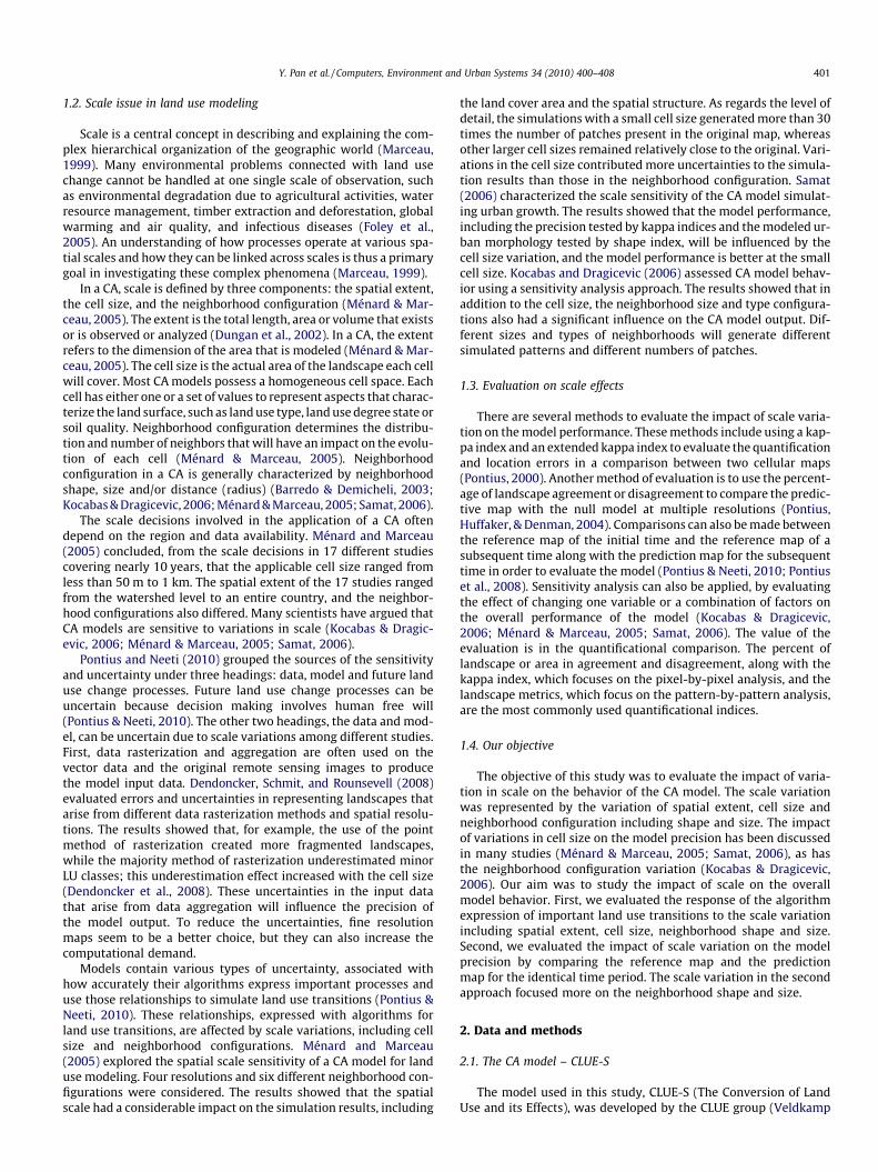
Fig. 5 depicts six spatial simulation results from Miyun Countyusing ring neighborhoods and the actual spatial distribution ofland use types in Miyun County in 2004. The kappa coefficient isused to measure the accuracy of the simulation results and, during

this study, to evaluate each simulation result by comparing the re-sults with the actual map of the model target year 2004. The calcu-lations of the kappa index were executed by the confusion matrixmodule of the ENVI4.4 software.

For both the ring and scope neighborhood shape types, the sim-ulation precision varied due to the neighborhood size variation(Fig. 6). The general trend is a decrease in precision with increasingneighborhood size when using the ring neighborhood shape type.When using scope-shaped neighborhoods, the precision increasesto a maximum when the neighborhood size increases to 7 � 7 cells,and then a decreasing trend is observed. In comparing the twocurves, the resulting precision using scope neighborhoods of anyneighborhood size is higher than the resulting curve using a ringshape neighborhood. An exception is seen with the neighborhoodsize of 3 � 3 cells, where the shapes of the two neighborhood typesare the same (Fig. 1).

In the model used herein, and within the neighborhood, theland interacts with its neighbors with the same weight of effects,independent of the positions or directions of the neighbors. As longas the scope is just outside the definition of the neighborhood witha particular size, and assuming that there is no interaction, theneighbors just beyond the edge of the neighborhood will bedefined.

In most cases, the interactions become weaker as the distanceincreases, based on the theory of distance-decay effects (Smith,1976). It is assumed that the near neighbors with strong interac-tions are important to the status or the change of the land. Thisrelationship, in our case, means that for new construction land,the existing construction land is the most attractive neighbor forthe small neighborhood size scenario. We therefore declare theself-organization as the most important function. If the neighbor-hood size increases to 11 cells or 13 cells (Fig. 4a curve of arable

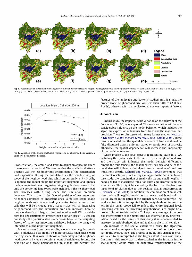
Fig. 5. Result maps of the simulation using different neighborhood sizes for ring shape neighborhoods. The neighborhood size for each simulation is: (a) 3 � 3 cells, (b) 5 � 5cells, (c) 7 � 7 cells, (d) 9 � 9 cells, (e) 11 � 11 cells, and (f) 13 � 13 cells. (g) The actual map of year 2004, and (h) the actual map of year 1991.

0.612

0.614

0.616

0.618

0.620

0.622

0.624

0.626

3 5 7 9 11 13Neighbourhood size (amount of cells)

Kapp

a co

effic

ient

Ring Scope

Location: Miyun; Cell size: 200 m

Fig. 6. Variation of the kappa coefficient response to neighborhood size variationusing two neighborhood shapes.

Y. Pan et al. / Computers, Environment and Urban Systems 34 (2010) 400–408 407

– construction), the arable land starts to depict an appealing effectto new construction land. We assume that the arable land attrac-tiveness was the less important determinant of the constructionland expansion. During the simulation, as the smallest ring orscope of the neighborhood size, which in our study is 3 � 3 cells,is applied, the model favors the important neighbors and ignoresthe less important ones. Large-sized ring neighborhoods mean thatonly the borderline land types were included. If the neighborhoodsize increases with a ring shape, the simulation precisiondecreases. This is due to the favored position of less importantneighbors compared to important ones. Large-size scope shapeneighborhoods are characterized by a central to borderline extentcells that will be included. For a scope shape with an increasingneighborhood size, the simulation precision increases becausethe secondary factors begin to be considered as well. With a neigh-borhood size enlargement greater than a certain size (7 � 7 cells inour study), the precision starts to decrease because the weightingfactors of many less important neighbors balance the weight ofinteractions of the important neighbors.

As can be seen from these results, scope shape neighborhoodswith a moderate size might be more accurate than those withthe ring shape. It is wise to choose a moderately-sized neighbor-hood scope to include a certain amount of neighbors. Second, thebest size of a scope neighborhood must take into account the

features of the landscape and patterns studied. In this study, theproper scope neighborhood size was less than 1400 m (200 m �7 cells); otherwise, it may involve too many less important factors.

4. Conclusion

In this study, the impact of scale variation on the behavior of theCA model (CLUE-S) was explored. The scale variation will have aconsiderable influence on the model behavior, which includes thealgorithm expression of land use transitions and the model outputprecision. These results agree with many former studies (Kocabas& Dragicevic, 2006; Ménard & Marceau, 2005; Samat, 2006). Theseresults indicated that the spatial dependence of land use should befully discussed across different scales or resolutions of analysis,otherwise, the spatial dependence will increase the uncertaintyof the model outcomes.

More precisely, the four aspects representing scale in a CA,including the spatial extent, the cell size, the neighborhood sizeand the shape, will influence the model behavior differently.Among the four aspects, the spatial extent, cell size and neighbor-hood size will influence the algorithm’s expression of land usetransitions greatly. Ménard and Marceau (2005) concluded thatthe finest resolution is not always an appropriate decision. In ourcase study, the combination of small cell size and small neighbor-hood size led to inaccurate transition rules and incorrect land usesimulations. This might be caused by the fact that the land usetypes tend to cluster due to the positive spatial autocorrelation(Overmars et al., 2003). In addition, the combination of small cellsizes and small neighborhood sizes can create a neighborhood thatis still located in the patch of the original particular land type. Theland use transitions interpreted by the neighborhood interactionwithin this small scope fail to reflect the entire regional level.Increasing cell size or increasing neighborhood size might be aproper solution to this problem. To keep the advantage of the pre-cise interpretation of the actual land use information by fine reso-lution, based on the results of this study it is recommended toincrease the neighborhood size and maintain the small cell size.

An increase in the spatial extent will cause the algorithmexpression of some special land use transitions of hot spots to re-vert to the average level. The process of arable land change to orch-ard failed to be interpreted in the larger extent in our case study.Our aim in this study was to detect whether the increase in thespatial extent would cause the qualitative transformation of the

408 Y. Pan et al. / Computers, Environment and Urban Systems 34 (2010) 400–408

algorithm expression of land use transitions. However, we recom-mend, in future research, including scenarios on continued in-creases in spatial extent, which might be helpful to evaluate towhat extent the variation of spatial extent will cause a qualitativetransformation of land use transitions expression.

Many studies have concluded that the model output precisionwould also be affected by cell size variation (Kocabas & Dragicevic,2006; Ménard & Marceau, 2005; Samat, 2006). In our study, we at-tempted to further explore the impact of neighborhood size andshape variation on the model output precision. The neighborhoodsize and shape variation affect the model output precision. If theneighborhood size increases with ring shape, the simulation preci-sion decreases. For a scope shape with increasing neighborhoodsize, the simulation precision will first increase and then decreasewhen the size is larger than a certain value (7 � 7 cells in thisstudy). The average precision for each neighborhood size of scopeshape was higher than for ring shaped neighborhoods. However,the scope-shaped neighborhood may also smooth the definitionof land use change (Barredo & Demicheli, 2003; de Nijs, de Niet,& Crommentuijn, 2004). These problems could be solved by usinga multi-ring neighborhood (Duan et al., 2004; White & Engelen,2000). The near ring neighbors can be assigned with high weights,and the farther ring can be assigned with less weight. However,this multi-ring neighborhood will also potentially increase thecomplexity and uncertainty of the model.

A proper set of scale parameters recommended in our caseconsists of a possible finest resolution of 25 m and a neighborhoodsize of 9 � 9 cells with a scope shape. This scale type parameter setreflects the most accurate land information and the best interpreta-tion of land use transitions achieving the highest model precision.For different model applications at different spatial scales, a preli-minary discussion of the scale parameter setting is recommended.

Acknowledgements

This paper is based on both the Research Project(2006BAJ10B05) supported by the Chinese Ministry of Scienceand Technology, and on the First Sino-German International Re-search Training Group (IRTG) – Sustainable Resource Use in NorthChina, jointly supported by the German Research Council(GRK1070, DFG) and the Chinese Ministry of Education. We alsothank Dr. P.H. Verburg and Dr. Zengqiang Duan for helpful sugges-tions and provision of the CLUE-S model and the three anonymousreviewers for their very useful comments.

References

Barredo, J. I., & Demicheli, L. (2003). Urban sustainability in developing countries’megacities: Modeling and predicting future urban growth in Lagos. Cities, 20,297–310.

Barredo, J. I., Kasanko, M., McCormick, N., & Lavalle, C. (2003). Modelling dynamicspatial processes: Simulation of urban future scenarios through cellularautomata. Landscape and Urban Planning, 64, 145–160.

Clarke, K. C., Hoppen, S., & Gaydos, L. (1997). A self-modifying cellular automatonmodel of historical urbanization in the San Francisco Bay area. Environment andPlanning B: Planning and Design, 24, 247–261.

CLSPI (2005). The project of constructing land survey data base. Bureau of Chinaland surveying and planning. <http://www.clspi.org.cn>.

de Nijs, T. C. M., de Niet, R., & Crommentuijn, L. (2004). Constructing land-use mapsof the Netherlands in 2030. Journal of Environmental Management, 72, 35–42.

Dendoncker, N., Schmit, C., & Rounsevell, M. (2008). Exploring spatial datauncertainties in land-use change scenarios. International Journal ofGeographical Information Science, 22(9), 1013–1030.

Duan, Z., Verburg, P. H., Zhang, F., & Yu, Z. (2004). Construction of a land-use changesimulation model and its application in Haidian District, Beijing. Acta GeograSinica, 59, 1037–1047 [in Chinese].

Dungan, J. L., Perry, J. N., Dale, M. R. T., Legendre, P., Citron-Pousty, S., Fortin, M.-J.,et al. (2002). A balanced view of scale in spatial statistical analysis. Ecography,25, 626–640.

Foley, J. A., DeFries, R., Asner, G. P., Barford, C., Bonan, G., Carpenter, S. R., et al.(2005). Global consequences of land use. Science, 309, 570–574.

Fonstad, M. A. (2006). Cellular automata as analysis and synthesis engines at thegeomorphology–ecology interface. Geomorphology, 77, 217–234.

Kocabas, V., & Dragicevic, S. (2006). Assessing cellular automata model behaviorusing a sensitivity analysis approach. Computers, Environment and UrbanSystems, 30, 921–953.

Lambin, E. F., Baulies, X., Bockstael, N., Fischer, G., Krug, T., Leemans, R., et al. (1999).Land-use and land-cover change: Implementation strategy, IGBP Report No. 48/IHDP Report No. 10. Stockholm: IGBP. p. 125.

Marceau, D. (1999). The scale issue in social and natural sciences. Canadian Journalof Remote Sensing, 25(4), 347–356.

Ménard, A., & Marceau, D. J. (2005). Exploration of spatial scale sensitivity ingeographic cellular automata. Environment and Planning B: Planning and Design,32(5), 693–714.

Overmars, K. P., de Koning, G. H. J., & Veldkamp, A. (2003). Spatial autocorrelation inmulti-scale land use models. Ecological Modelling, 164, 257–270.

Pontius, R. G. Jr., (2000). Quantification error versus location error in comparison ofcategorical maps. Photogrammetric Engineering & Remote Sensing, 66(8),1011–1016.

Pontius, R. G., Jr., & Neeti, N. (2010). Uncertainty in the difference between maps offuture land change scenarios. Sustainability Science., 5, 39–50.

Pontius, R. G., Jr., Boersma, W., Castella, J. C., Clarke, K., de Nijs, T., Dietzel, C., et al.(2008). Comparing the input, output, and validation maps for several models ofland change. Annals of Regional Science, 42(1), 11–47.

Pontius, R. G., Jr., Huffaker, D., & Denman, K. (2004). Useful techniques of validationfor spatially explicit land-change models. Ecological Modelling, 179(4), 445–461.

Samat, N. (2006). Characterizing the scale sensitivity of the cellular automatasimulated urban growth: A case study of the Seberang Perai Region, PenangState, Malaysia. Computers, Environment and Urban Systems, 30, 905–920.

Schneider, L. C., & Pontius, R. G. Jr., (2001). Modeling land-use change in the Ipswichwatershed, Massachusetts, USA. Agriculture, Ecosystems and Environment, 85,83–94.

Smith, T. E. (1976). Spatial discounting and the gravity hypothesis. Regional Scienceand Urban Economics, 6, 331–356.

Tomlin, C. D. (1990). Geographic information systems and cartographic modeling.Englewood Cliffs, NJ: Prentice Hall [In ‘journal’ Verburg, P. H., de Nijs, T. C. M.,van Eck, J. R., Visser, H., de Jong, K. (2004). A method to analyse neighborhoodcharacteristics of land use patterns. Computers, Environment and Urban Systems,28, 667–690].

Turner II, B. L., Skole, D. L., Sanderson, S., Fischer, G., Fresco, L. O., Leemans, R. (1995).Land-use and land-cover change. Science/research plan. IGBP Report No. 35 andHDP Report No. 7, Stockholm and Geneva. p. 132.

Veldkamp, A., & Fresco, L. O. (1996). CLUE: A conceptual model to study theconversion of land use and its effects. Ecological Modelling, 85, 253–270.

Verburg, P. H., de Koning, G. H. J., Kok, K., Veldkamp, A., & Bouma, J. (1999). A spatialexplicit allocation procedure for modelling the pattern of land use change basedupon actual land use. Ecological Modelling, 116, 45–61.

Verburg, P. H., de Nijs, T. C. M., van Eck, J. R., Visser, H., & de Jong, K. (2004). Amethod to analyse neighborhood characteristics of land use patterns.Computers, Environment and Urban Systems, 28, 667–690.

Verburg, P. H., Eickhout, B., & van Meijl, H. (2008). A multi-scale, multi-modelapproach for analyzing the future dynamics of European land use. Annals ofRegional Science, 42, 57–77.

Verburg, P. H., Soepboer, W., Veldkamp, A., Limpiada, R., Espaldon, V., & Mastura, S.(2002). Modeling the spatial dynamics of regional land use: The CLUE-S model.Environmental Management, 30, 391–405.

Verburg, P. H., van Eck, J. R., de Nijs, T. C. M., Dijst, M. J., & Schot, P. (2004).Determinants of land-use change patterns in the Netherlands. Environment andPlanning B: Planning and Design, 31, 125–150.

Wagner, D. F. (1997). Cellular automata and geographic information system.Environment and Planning B: Planning and Design, 24(2), 219–234.

White, R., & Engelen, G. (2000). High-resolution integrated modeling of the spatialdynamics of urban and regional systems. Computers, Environment and UrbanSystems, 24, 383–400.

Wu, J. G. (2004). Effects of changing scale on landscape pattern analysis: Scalingrelations. Landscape Ecology, 19, 125–138.

Wu, J. G., Shen, W. J., Sun, W. Z., & Tueller, P. T. (2002). Empirical patterns of theeffects of changing scale on landscape metrics. Landscape Ecology, 17, 761–782.