the impact of a national minimum wage on the … · the impact of a national minimum wage on the...
TRANSCRIPT

The impact of a national minimum wage on the South Africa economy
Asghar Adelzadehand
Cynthia AlvillarJuly 2016
Working Paper Series, No. 2National Minimum Wage Research Initiative
www.nationalminimumwage.co.za
University of the Witwatersrand

i
Abstract
In South Africa today, nearly 50 percent of the population lives in poverty, the Gini-‐coefficient is close to 0.7, and almost one third of full-‐time workers earn less than R2 500 a month. As the South African government considers introducing a national minimum wage (NMW) to spark an economic growth path with lower inequality and poverty, we provide an impact analysis of alternative NMW scenarios. While linked macro-‐micro models have been used internationally, including in South Africa, to examine the potential impact of minimum wages, they have predominantly relied on computable general equilibrium (CGE) techniques to produce projections of employment, wages and prices. However, empirical CGE models have been extensively criticised in the literature from analytical, functional and numerical perspectives, raising serious doubts about the validity of their assessments of the potential impact of policies such as the national minimum wage. We utilise DIMMSIM which links a multi-‐sector macro econometric model of South Africa with a full household micro-‐simulation model of the country to capture the dynamic two-‐way interactions between the macroeconomic performance and household level poverty and income distribution. Our results include: A NMW in South Africa can potentially yield positive overall macro-‐ and micro-‐economic outcomes, when taking into account direct, indirect and dynamic responses in the labour market, income, expenditure, prices, and production. It has the potential to meaningfully achieve its core goals of reducing poverty and income inequality, especially among bottom household quintiles. The net effect of the NMW includes an upward shift of aggregate demand (due to increased income and expenditure of more than four million full-‐time workers) and an outward shift of aggregate supply (due to improved labour productivity), thus spurring modest stable macroeconomic growth. The policy will directly and indirectly stimulate demand for and output of economic sectors, especially in manufacturing. For more than 85 percent of economic sectors, the positive employment impacts of sector output increases outweigh the direct relatively small negative employment impact of marginally higher sectoral average real wage rates.
Key words: national minimum wage, South Africa, linked macro-‐micro model, econometric modelling, poverty, inequality.
Authors and Acknowledgements
Asghar Adelzadeh is Director and Chief Economic Modeller at Applied Development Research Solutions (ADRS). Email: asghar@adrs-‐global.com.
Cynthia Alvillar is CEO and Senior Labour Market Specialist at ADRS. Email: c.alvillar@adrs-‐global.com
The authors would like to express their gratitude to the Friedrich-‐Ebert-‐Stiftung (FES) of South Africa for providing financial support for this project. We also thank Gilad Isaacs, Ilan Strauss, Alan Manning, Mike Rogan, Arden Finn, Jeremy Seekings and many participants at the National Minimum Wage Symposium hosted by CSID, the seminar participants at the UCT economics department, UWC economics department, the Parliamentary Budget Office, and the South African Revenue Service, and the NEDLAC constituencies for their valuable comments and suggestions on the earlier presentations of the findings of this study. Any
opinions and conclusions expressed herein are those of the authors.

ii
Table of Contents
1. Background .............................................................................................................................. 1
2. Literature review ................................................................................................................... 2
3. Basic structure and features of DIMMSIM ..................................................................... 5 3.1. DIMMSIM’s macroeconomic component ................................................................. 6 3.2. Model Specification ....................................................................................................... 10 3.3. MEMSA Data Sources and Preparation .................................................................. 11 3.4. Parameter Estimation Method .................................................................................. 12 3.5. DIMMSIM’s microsimulation component .............................................................. 21 3.6. Accounting consistency within DIMMSIM ............................................................. 21 3.7. Macro-‐micro interactions in DIMMSIM .................................................................. 22
4. National minimum wage scenarios ................................................................................ 23 4.1. Base or “Business-‐as-‐Usual” scenario .................................................................... 23 4.2. NMW scenario 1: the ‘Minimal’ scenario ............................................................... 24 4.3. NMW scenario 2: the ‘Index 40%’ scenario .......................................................... 24 4.4. NMW scenario 3: the Index 45% scenario ............................................................ 25 4.5. NMW scenario 4: the ‘Maximal’ scenario ............................................................... 26
5. National minimum wage module .................................................................................... 26
6. Structure of sector employment ..................................................................................... 27
7. Analysis of results ................................................................................................................ 29 7.1. National minimum wage and sector shocks ......................................................... 30 7.2. Wage effect ...................................................................................................................... 32 7.3. Household income effect ............................................................................................. 34 7.4. Household consumption effect ................................................................................. 35 7.5. Growth effect ................................................................................................................... 37 7.6. Employment effect ........................................................................................................ 41 7.7. Labour productivity effect .......................................................................................... 46 7.8. Inflation effect ................................................................................................................ 47 7.9. Inequality and poverty effects .................................................................................. 48 7.10. Comparison of NMW scenario performances .................................................... 53
8. Conclusion .............................................................................................................................. 53
References ...................................................................................................................................... 56

1
1. Background “We need to ensure that the benefits of growth are more equitably shared. We need to confront poverty and inequality…We need to examine and understand income inequality, and develop measures to reduce it. Among other things, we need to examine the value and possible challenges of implementing a national minimum wage.”
-‐-‐Address by Deputy President Cyril Ramaphosa at the 19thNEDLAC Annual Summit, 5 September 2014
“The NEDLAC constituencies recognize: [2.2.3] that unemployment and underemployment, including the legacy of low wages, are the biggest causes of poverty and inequality in South Africa…Therefore, the NEDLAC constituencies resolve to: [2.2.6] engage on the modalities of introducing a national minimum wage in South Africa.”
-‐-‐EKURHELENI DECLARATION, NEDLAC Declaration of the Labour Relations Indaba, Promoting Employment and Strengthening Social Dialogue: Towards Transformation of the South African
Labour Relations Environment, 4 November 2014
To even the casual observer, there is no doubt that the notion of a national minimum wage is a politically contentious issue. It always has been. When it was first introduced in South Africa as a goal of workers in the 1930s, articulated in the Freedom Charter, and reiterated again in the era of transformation, it was intended as a means to level the playing field for workers at the bottom of the income distribution.
More than 20 years into South Africa’s new democracy, the instruments for wage determination in the labour market have yet to lift all workers out of poverty and yield a more equitable distribution of wealth. Successive rounds of initiatives, efforts, discussion and debate to spur growth have taken place, often targeting the labour market as the chief obstacle to a desired trajectory, or pinning hopes on its deregulation to unleash employment creation, investment, growth and economic stability. Though it is abundantly clear that labour market transformation has always been a key prerequisite to the new dispensation promised by post-apartheid South Africa, apartheid’s legacy of poverty, discrimination and inequality has proven difficult to dismantle.
In recent years, the government has given impetus to overcoming the constraining three-headed hydra of poverty, unemployment, and inequality in order to improve the economic position of the working poor and their families, and to improve economic outcomes for the economy as a whole. Importantly, discussion and debate among stakeholders, including constituent representatives at NEDLAC have embarked on structured engagement that has the potential to move the process forward. However, as the stakeholders at the bargaining table can attest, adherents and detractors often have visceral reactions to calls for a national minimum wage, often without ample information or understanding of the full effects that such a policy could have. This report attempts to fill that void by examining the consequences of introducing a national minimum wage in South Africa.
To interrogate and understand the impact of a national minimum wage policy, economic modelling techniques are used to quantify the potential impact of introducing a national minimum wage in South Africa. The ADRS Dynamically Integrated Macro-Micro Simulation Model of South Africa (DIMMSIM) is the model used to run simulations on alternative minimum wage scenarios, and to generate forecasts of likely impacts on a range of

2
macroeconomic variables and poverty and inequality indicators. The findings are presented below.
This report thus examines the likely consequences of introducing a national minimum wage in South Africa. In order to do so, it will first review representative literature, before proceeding to describe the report’s empirical methodology. We then describe the minimum wage scenarios that are tested followed by an analysis of the simulation’s results and concluding remarks. The goal of the paper is not only to assess the potential impact, but ultimately to help assess whether instituting a national minimum wage is good economic policy.
2. Literature review During the last 30 years, poverty analysis and the challenge of designing ‘pro-‐poor’ policies have gradually occupied the central attention of development research.1 This is partly attributed to worsening inequality and the persistence of high rates of poverty in many parts of the world. An important dimension of the current research, which has received particular attention from economic modellers, is increased recognition of the need for a better understanding of the interactions between macroeconomic dynamics and household level poverty and inequality. As Bourguignon et al. (2008) point out, macro models do not account for the poverty and distribution effects of policy changes at the household level, and micro models cannot explain the impact of macroeconomic policy changes on poverty.
While new techniques have been developed to use economic modelling as a tool for designing concrete and country-‐specific pro-‐poor policies, awareness is mounting that the effects of policies need to be traced to changes in the income and expenditure of individuals and households, and that changes in household welfare has an important bearing on economic growth. Thus, economic models have been developed to capture the interactions between the macroeconomy and household poverty and inequality. This improvement has paved the way for a more holistic approach to the design of anti-‐poverty policies. Pioneering works in the early 1980s by Dervis et al. (1982), and Gunning (1983) paved the way for a significant leap in linking household level poverty-‐distribution analysis and the dynamics of the macroeconomy through what is now known as linked macro-‐micro modelling.2
The range of linked macro-‐micro techniques is varied and has expanded over time.3 There are at least four categories of linked macro-‐micro models. The main distinction between the four rests on the technique used to either represent households in the model or to extend the scope and nature of the dynamic interactions between
1 Kakwani and Pernia (2000) define pro-‐poor policies as policies that are deliberately biased in favour of the poor so that the poor benefit proportionately more than the non-‐poor. 2 The idea of linking micro and macroeconomic simulation models goes back to Orcutt (1967). The next set of important contributions in this area include: Thorbecke (1991), Bourguignon et al. (1991), de Janvry et al. (1991) and Morrisson (1991). More recent contributions include Decaluwe et al. (1999a) and Decaluwe et al. (1999b), Cogneau and Robilliard (2000), Agenor et al. (2003), Cockburn (2001), Bourguignon et al. (2003), and Savard (2003). 3 Estrades (2013) reviews the different linked macro-‐micro techniques and presents a brief description of their pros and cons.

3
macroeconomics and households.4 The first approach is the traditional CGE modelling technique that utilises a small number of representative households5 to capture households in their design. Though it is widely used, the main shortcomings of this approach are generally that it assumes no changes in intra-‐group income distribution or imposes restrictions on the distribution. The second type of model is a variation of the first with the incorporation of a larger number of representative households into the CGE. This is an attempt to better represent the existing socioeconomic stratification within the population.6 Examples of this approach are found in the work of Decaluwe et al. (1999b) and Cockburn (2001). This approach clearly avoids the problem of selecting ‘representative households’ and, furthermore, allows for detailed analyses of distribution and poverty. However, as Piggot and Whalley (1985) point out, there are important intra-‐group heterogeneities that a high number of representative households do not capture. The third approach combines microsimulation modelling techniques, pioneered by Orcutt et al. (1961), with CGE modelling to further enhance the rigour and flexibility of household behaviour in the overall model. Examples of this approach include Bourguignon et al. (2003).
Traditional CGE models with ‘representative households’ allow feedback effects from household behaviour but given the significant heterogeneity between households, this approach’s usefulness for the purpose of pro-‐poor policy design is severely limited. On the other hand, most CGE models that incorporate large household surveys do not capture two-‐way interactions between the economy and households. This clearly weakens their overall appeal within the current development discourse since they fall into the traditional approach of allowing the macroeconomy to influence income distribution and poverty, but do not allow changes in income distribution and poverty to influence macroeconomic performance.
Savard (2003) represents a fourth approach within the CGE framework. His work aims to overcome some of the shortcomings of the previously described approaches inasmuch as his model is designed to keep the feedback mechanism between households and the economy while using microsimulation techniques for households. He addresses some of the issues related to the coherence between the household model and the CGE model, introduces two-‐way links between the two, and develops an approach to achieve convergence between the results from the two models.
In practice, international applications of linked macro-‐micro modelling techniques have predominantly relied on empirical CGE approaches to represent the working of the economy. Similarly, in South Africa, CGE-‐based linked macro-‐micro techniques have been used for policy analyses, including minimum wage studies. These models have relied on CGE techniques to produce projections of employment, wages and prices that are transmitted to the micro component of the model to estimate the poverty and distribution impact.7
4 The following review uses Savard (2003). 5 See for example Dervis et al. (1982), de Janvry et al. (1991) and Agenor et al. (2003). 6 The three commonly used criteria to disaggregate households in a social accounting matrix are geographical location, household resources, and occupation of the head of household (Thorbecke 2000). 7 Pauw and Leibbrandt (2012) use a linked CGE micro model to study the impact of a national minimum wage in South Africa. The National Treasury, MacLeod (2015), has also used the CGE based linked macro-‐micro model that was developed by Pauw (2007) and Alton et al. (2012) to examine the impact of the

4
Yet, empirical CGE models have been extensively criticised in the literature from analytical, functional and numerical perspectives. The analytical criticisms centre on the theoretical foundation of CGE models which informs the specification of variables used in the models and their causal relationships. Since CGE models are quantitative expressions of neo-‐classical general equilibrium theory, they embody strong theoretical assumptions about the working of the economy that do not necessarily reflect the reality of market economies, especially those in developing economies. These assumptions include perfect competition and flexible markets with inherent tendencies to self-‐correct and achieve full employment general equilibrium, i.e. to simultaneously clear all goods and factor markets. These assumptions are among CGE’s highly debatable depiction of the working of the economy. De Canio (2003) and Ackerman (2002) review these assumptions, Barker (2004) examines their influence on the development of CGE models, and Taylor et al. (2006) provides a critique of CGE models as used in studies of the impact of trade liberalisation.
Another set of criticisms of CGE models centres on the calibration method used to develop the model’s parameters (i.e., elasticities). The method is a deterministic approach to calculating parameter values from a benchmark equilibrium data set. Shoven and Whalley (1992) point out that the techniques are less than ideal and undermine the reliability of the results derived from the model since the parameters are arbitrary, based on the empirical literature, or are a set of values that “force the model to replicate the data of a chosen benchmark year.” Similarly, Jorgensen (1984), Lau (1984), Jorgensen et al. (1992), and Diewert and Lawrence (1994), among others, point out flaws they have found in the parameter setting techniques in CGE models. This includes the use of industry or commodity level elasticities that are methodologically inconsistent, and/or are from other countries, and/or are old and obsolete estimates, and/or are outright guesses.8 They correctly point out that without reliable or credible parameter values, the utility of the empirical CGE models is compromised. Since calibration is a process through which a model’s parameters are adjusted until the model reproduces the national account for the benchmark year, the quality of the data is critical. Yet, one year of data, which empirical CGE models are usually built upon, provides insufficient grounds upon which to base generalised results. Thus, an important criticism regarding the inherently limited scope of CGE models hinges on the calibration technique itself, which causes the quality of the model to be at least partly dependent on the quality of the data for an arbitrarily chosen benchmark year. Critics also note that the calibration techniques are susceptible to errors and biases as a result of subjecting the data matrices to various scaling processes to force micro-‐consistency. These errors and biases will directly influence the parameters of a calibrated model.9 Another important criticism of the CGE model’s calibration approach is that it tends to be based on a ‘one-‐size-‐fits-‐all’ approach to all industries by using the Constant NMW. Bhorat et al. (2015) refers to the use of a CGE model for its examination of the feasibility of a NMW for South Africa. However, the specifics of the model have not been provided. 8 The “expediencies” they identify include the use of “elasticities estimated for commodity and/or industry classifications which are inconsistent with those maintained in the model, and/or for countries other than the one(s) represented by the model, and/or obsolete estimates from past literature, not to mention outright guesses when no published figures are available.” 9 See Mansur and Whalley (1984) and Lau (1984) for an extensive review of the calibration method.

5
Elasticity of Substitution (CES) class of functions. Utilising restrictive assumptions about the industry elasticities not only have a bearing on the way in which industries are incorporated into the model but also on the validity of the results derived. McKitrick (1998) demonstrates that changing from CES functions to flexible forms modifies the performance of a CGE model so much that the two models seem to represent entirely distinct descriptions of the economy. He finds that the choice of functional forms influences both industry-‐specific results and aggregate results, even for small policy shocks. McKitrick (1998) calls the above critique of the functional and numerical structure of calibrated CGE models the ‘econometric critique’ of CGE modelling, which is separate from criticisms directed at the analytical structure of these models. These critiques raise serious doubts about the validity of the functional and numerical structures of calibrated CGE models that are currently being used, including the CGE models used in South Africa. The econometric critique of CGE modelling provides a priori reasons for doubting the validity of the functional and numerical structures of many CGE models used in South Africa and raises serious questions about both their industry-‐specific and aggregate results. It is the combination of both the underlying theoretical assumptions of CGE models, e.g. perfect competition and general equilibrium, and their functional and empirical shortcomings that raises serious questions about the utility of empirical CGE models for analysis of the proposed national minimum wage policy in South Africa. In this paper, we utilise a linked macro-‐micro model of South Africa that is neither based on the neo-‐classical theory of perfect competition and general equilibrium nor uses calibration methods to develop the model’s parameters. The Dynamically Integrated Macro-‐Micro Simulation Model (DIMMSIM) links a multi-‐sector macroeconometric model of South Africa with a household microsimulation model of the country to capture the dynamic two-‐way interactions between the macroeconomic performance and household level poverty and income distribution. DIMMSIM’s analytical approach is in the tradition of pluralism of heterodox economics and uses modern time-‐series specification and estimation methods to estimate the parameters of the model’s behavioural equations.
The substantial theoretical, functional and empirical differences between DIMMSIM and CGE-‐based models translate into critical differences of how a NMW transmits and impacts the economy and its sectors. The methodological differences between the two types of modelling also lead to key differences in the interpretation of results and to potentially different conclusions.
3. Basic structure and features of DIMMSIM The Dynamically Integrated Macro-‐Micro Simulation Model (DIMMSIM) is one of the four economic models of South Africa built by Applied Development Research Solutions and available on the ADRS website through their user-‐friendly web-‐platforms

6
(www.adrs-‐global.com).10 DIMMSIM integrates a macroeconometric model of South Africa with a household microsimulation model of the country to capture the dynamic interactions between the macroeconomic performance and the poverty and income distribution at household level. Following is a brief introduction to the DIMMSIM’s two underlying models.
3.1. DIMMSIM’s macroeconomic component One of the two economic models that underlie DIMMSIM is the non-‐linear Macroeconometric Model of South Africa (MEMSA) that captures the structure and the working of the South African economy. It allows design and analyses of macroeconomic and industrial policies and produces projections of the paths of key indicators related to the economy and its economic sectors under various domestic and international contexts and policy options.
MEMSA is a bottom-‐up model with more than 3200 equations that captures the structure of the National Income and Product Account (NIPA) at sector and aggregate levels and produces projections that are consistent with various national accounting identities in nominal and real terms. The model includes more than 400 estimated equations that analytically and empirically capture the behaviour of the private and household sectors as part of capturing the working and dynamics of the economy from its production, expenditure and income perspectives. DIMMSIM’s equation system (Figures 1 and 2) can be broken down into a number of blocks that include:
§ The Final Demand Block encompasses 769 equations. It includes sets of estimated equations that capture the behaviour of the private sector as it relates to sectoral-‐level investment, exports, and imports in 45 sectors; households in terms of expenditure on 27 categories of consumption goods and services; and the public sector in terms of final consumption expenditure and investment. The expenditure block of equations therefore produces projections of various components of aggregate demand in the economy that facilitate the model’s projection of real and nominal GDP from the expenditure side.11
§ The Production Block includes 712 equations that represent sector and aggregate production-‐related activities in the economy. It includes sets of equations that produce projections of sector outputs, potential outputs, capital stock, and capital productivity, all in nominal and real terms. Private sector decisions on how much to produce in various sectors of the economy are captured through 40 estimated equations that link the decisions to various demand, supply and price factors in the economy. Therefore, the equations of the production block generate consistent projections of nominal and real values for sector and aggregate outputs, i.e., value added at basic prices. The aggregate of
10 The list of ADRS’ current models of South Africa include: multi-‐sector macroeconometric model of South Africa (MEMSA); linked macro-‐micro models (DIMMSIM); linked macro-‐education model (LM-‐EM); provincial macroeconomic models (NPMM); social security models; direct and indirect tax models; poverty-‐inequality models; public employment models; and an economy-‐energy-‐emissions model. 11 GDP from the expenditure side is the sum of final consumption expenditure by households and general government, gross investment, exports and imports of goods and services, and the GDP residual item.

7
sectoral value added at basic prices plus the net taxes and subsidies on products provide the model’s annual projections of GDP from the production side.12
§ The Price and Wage Block is comprised of 413 equations that include time-‐series estimated behavioural equations for sector output prices (45), consumer prices (30), and investment prices (45). It also includes equations for sector import and export prices, sector and economy-‐wide inflation rates, and 45 estimated equations for the sector-‐level real wage rate (i.e., average remuneration rates) and 45 calculated sectoral-‐level nominal wage rates.
§ The Labour Market Block is comprised of 186 equations that include 40 estimated equations that capture factors that determine short-‐ and long-‐term demand for sector-‐level employment. In addition, this block includes equations for sectoral labour productivity, labour force, unemployment rate, and other labour market indicators.
§ The Income, Expenditure, and Savings Block includes 569 equations that capture a detailed breakdown of income, expenditure, and saving of households, incorporated businesses and government, in both nominal and real terms. A combination of variables from this block, the labour market block, the price and wage block, and the production block provide forecasts of the real and nominal GDP from the income side.13
§ The Financial Block embodies 88 equations for indicators related to the financial and monetary side of the economy, such as the interest rate, exchange rates, money supply, credit extensions, household financial assets and liabilities, and foreign direct and portfolio investments. The financial block variables are especially important determinants of variables in other equation blocks and include policy variables and time-‐series estimated variables.
§ The National Account Block incorporates more than 470 equations. This block of equations is responsible for ensuring consistency and enforcing national-‐income and product-‐account relationships within the economic system captured by the model. For example, it ensures that in the model, the calculation of GDP, both real and nominal, from the income, production and expenditure sides are comprised of relevant NIPA components and are consistent with each other at aggregate and sector levels, in nominal and real terms.
The model’s list of exogenous variables includes a number of domestic and international variables. Among exogenous inputs to the model are:
• General government and public corporation investment • Monetary and fiscal policy rules • Government current spending • Tax and subsidy rates
12 GDP from the production side is equal to the sum of sectoral value added at basic prices and net taxes on products. 13 GDP from the income side is calculated as the sum of gross value added at factor cost plus net taxes on production and products.

8
• Population • Oil prices • OECD annual growth rates • Sub-‐Saharan annual growth rates • U.S. interest and inflation rates
Figure 1: Dynamically Integrated Macro-‐Micro Model of South Africa (DIMMSIM)
TrrfffffffA Graphical Presentation of DIMMSIM South Africa
Final Demand Blocks (769 equations)
Consumption
Investment
Government
Output Blocks (712 equations)
GVA at basic prices
GVA at Market Prices GDP at Factor Cost
Labour Market Block
(186 equations)
Financial Block Monetary Policy
(88 equations)
Interest rates Exchange rates Money supply
Credit, Wealth, Debt Financial account
Long Term Blocks
Income/Expend/Savings Blocks
(569 equations)
Exports
Imports
Prices/Wages Blocks (413 equations)
Wage rates
Sector prices Consumption deflators Investment deflators
GDP deflator Consumer Price Index Producer Price Index
Inventory
Microsimulation Modules
Income Tax and Indirect Taxes Old Age Pension
Child Support Grant Disability Grant
Care Dependency Grant Care Giver Grant
Basic Income Grant Income/Expenditure/Saving
Poverty Income Distribution
Output
Accounting Consistency Blocks
(470+ equations)
Primary sector
Secondary sector
Tertiary sector
Households
Business
Government
Macroeconomic
Microeconomic
Linked Macro-Micro
Exogenous and Parameter Block
Population Oil price
Gold price OECD Growth Rate
Sub-Sahara Growth Rate U.S. Interest Rate
Import prices Policy variables
Policy parameters Other variables
Investment Consumption Employment
Exports & Imports Wage rate/Prices/Deflators
Source: Adelzadeh, A.. Applied Development Research Solutions (ADRS), www.adrs-global.com

9
The macroeconomic module of DIMMSIM generates annual forecasts of a relatively large number of aggregate, sector level, nominal and real variables and indictors. It includes indicators related to production, labour market, prices, wages, financial variables, and incomes and expenditures of households, businesses and government. The model’s projections are consistent across aggregation levels both in nominal and real terms. Key outputs of the model include projections of:
• Key macroeconomic indicators • Demand for employment and the real and nominal average wage rates for 45
economic sectors • Output, investment, exports, imports, wages, and prices for 45 economic sectors • Financial indicators such as the interest rate, credit extensions, and money
supply • Trade indicators • Income and expenditure indicators • Sustainability indicators • Labour market indicators • Production indicators • Demand (expenditure) indicators
Figure 2: Macro-‐Econometric Model of South Africa (MEMSA) Sectors
1. Agriculture, Forestry and Fishing2. Coal Mining3. Gold, uranium and ore mining4. Other mining
5. Food6. Beverage7. Tobacco8. Textiles9. Wearing Apparel10. Leather and Leather products11. Footwear12. Wood and wood products13. Paper and paper products14. Printing, publishing & recorded media15. Coke & refined petroleum products16. Basic chemicals17. Other chemicals & man made fibres18. Rubber products19. Plastic products20. Glass and glass products21. Non-‐metalic minerals22. Basic iron & steel23. Basic non-‐ferrous metals24. Metal products excl.machinery25. Machinery and equipment 26. Electrical equipment27. Tv, radio & communication equipment28. Professional & scientific equipment29. Motor vehicles, parts & accessories30. Other transport equipment31. Furniture32. Other industries
Primary Manufacturing Services
Model's Economic Sectorswith 7 variables for each sector
(output, employment, investment, exports, imports, prices, wage rates)
33. Electricity, Gas and water34. Building construction and engineering35. Wholesale, retail trade, catering &
accomodation services36. Transport, storage, and communication37. Financial services, business
intermediation, insurance & real estate38. Community, social & personal services39. Other services40. Households41. General government
Aggregate Sectors
42. Total primary (sum of sectors 1 to 4)43. Total manufacturing (sum of sectors 5 to 32)44. Total services (sum of sectors 33 to 41)45. Total economy (sum of sectors 1 to 41)

10
3.2. Model Specification
Specification refers to the selection of a model’s functional form, that is, specifying the perceived nature of relations between variables in the economy. In the case of macroeconomic models, model specification generally is based on a good theoretical and empirical knowledge of how an economy functions and evolves over time. A model’s specification therefore must include sufficient structural detail to approximate the system and its multiple interactions while ensuring conformity between economic theory and econometric test criteria. Finally, model specification should provide sufficient detail to generate forecasts and should include relevant policy variables and their transmission channels.
The specification of MEMSA can be described in terms of the specification of its time-‐series estimated behavioural equations and a large number of real and nominal accounting and other relationships that together constitute the overall model. Specification of MEMSA’s Behavioural Equations: The latest version of MEMSA includes more than 400 estimated behavioural equations. It is composed of industry-‐level specification of output, employment, investment, wage rate, export and import, investment prices, sector prices, and export and import prices. The rest of the model’s estimated equations include detailed specification of real private household consumption expenditure, consumption prices, credit extension, money supply, exchange rates and other behavioural equations of the model. Given the heterogeneity among sectors of the economy, for the specification of each sector level variable (e.g., employment, investment), we considered the broad theoretical and empirical literature on the subject. Therefore, the specification of the model’s behavioural equations avoids a priori imposition of one theoretical stand on the determination of a given sector level variable. The adapted broad specification approach is especially appropriate since the focus of MEMSA is not to test or assert the validity of a particular theoretical proposition, but to capture the potential differences in the law of motion (i.e., behavioural differences) among sectors of the economy, using a combination of econometric test criteria and economic theory.14
The model therefore has used the theoretical and empirical literature to identify a range of sector and economy-‐wide variables that are found significant in explaining the long-‐term trend and short-‐term fluctuations of the model’s behavioural equations. In general form, the specification of the model’s behavioural variables includes demand-‐side (d), supply-‐side (s), price and expectation variables:
( , , , , )tv v h j k q uY f s d p e x= [1]
Where:
tvY represents estimated variables in MEMSA with v=1,2,...,V;
hs represents supply side variables with h = 0,1,..,H;
14 At the same time, the adopted approach reduces the risk of working with mis-‐specified regression equations.

11
jd represents demand side variables with j = 1,2,...,J; kp represents various aggregate and sector level prices with k=0,1,…,K; qe represents various expressions of expectations with e=0,1,…, E; and ux represents other variables with u=0,1,…,U.
Space limitation does not allow a full presentation of the specification of all of MEMSA’s large number of estimated equations. Table 1 provides a summary list of variables used in the specification and estimation process and their classification as demand side, supply side, prices, expectation, and other variables. It is important to note that the classification of variables is for ease of presentation.
To provide an example of the procedure that was followed to specify and estimate particular blocks of economic variables, section 3.1.4 describes the process for estimating the model’s 41 sector employment equations.
Specification of MEMSA’s Non-‐behavioural Equations: A significant number of MEMSA equations are designed to capture a wide range of nominal-‐real conversions and accounting relationships at sector and aggregate levels and to ensure inter-‐temporal consistency. MEMSA’s iterative process of generating each period’s forecast ensures that the accepted simulation results for each period satisfies all the specified accounting relationships. For example, within MEMSA, the components of the product account add up, and the income and product sides of the accounts are equal. Moreover, the price-‐quantity relationships are consistent.
3.3. MEMSA Data Sources and Preparation The specification of the model’s equations informs the range and the detail of its data requirements. MEMSA, as a multi-‐sectoral macroeconometric model, uses extensive amounts of data as inputs. The model’s main sources of data for its endogenous variables include the Reserve Bank’s electronic historical National Income and Product Account (NIPA) dataset and Quantec’s industry database, which is based on Statistics South Africa data. The model’s datasets start from 1970. As part of building the model’s database, the process included cross-‐checking industry time-‐series data with the Reserve Bank time-‐series data in order to ensure data consistency. The Standard Industrial Classification (SIC) for agriculture, mining (comprising three sectors) and services (comprising seven sectors) is aggregated at the 2-‐digit SIC level. Manufacturing (comprising 28 sectors) is aggregated at the 3-‐digit level. The data for the model’s
Supply SideProductivity
Capital labour ratioTax rates
Table 1: Classification of Sample of Variables Used in Specification of
Government Expenditure Import prices
Income Exchange rates Debt/GDPInvestment Export prices
Imports Sector prices Profit expectations OutputConsumption Investment prices Output expectations Deficit/GDP
Demand Side Prices Expectations OthersExports Consumption prices Price expectations Employment

12
aggregate sector – primary, manufacturing, services and total economy – are the sum of data from relevant subsectors.
The model’s database of exogenous variables includes domestic and international economic and policy indicators whose values are not determined within the model but are either a necessary part of the national accounting of the South African open economy or found to have statistically significant impact on particular endogenous variables of the economy. This includes, for example, the growth rates of OECD countries and Sub-‐Saharan countries, oil prices, metal prices, the U.S. interest rate, foreign investment, population growth, etc. For these and other similar data, MEMSA uses various international databases, such as the electronic databases and publications of the International Monetary Fund, the World Bank, the OECD, the European Union, the African and Asian Development Banks, OPEC, and other similar sources.
3.4. Parameter Estimation Method
The parameter estimation process refers to the utilisation of historical data and suitable econometric techniques to establish the explicit forms of the model’s behavioural equations. The process is expected to yield theoretically acceptable and statistically significant values for the parameters of the model equations.
The range of available regression techniques has expanded with the evolution of econometrics and the availability of more and more data. Empirical literature has also expanded the choices that are available for estimating parameters of an economic model. For the specific functional form of its estimated equations, MEMSA uses the cointegration technique, in which relationships among a set of economic variables are specified in terms of error correction models (ECM) that allow dynamic convergence to a long-‐term outcome.15 The independent variables of the estimated equation act as the ‘long-‐run forcing’ variables for the explanation of the dependent variable.16 The cointegration technique has been the preferred method used globally to build national macroeconometric models.
Among the several such techniques available, MEMSA uses the Autoregressive Distributed Lag (ARDL) estimation procedure, developed by Pesaran (1997) and Pesaran et al. (1996, 1999). The advantages of this technique are that it offers explicit tests for the existence of a unique cointegrating vector, and, since the existence of a long-‐run relationship is independent of whether the explanatory variables are integrated of order one, I(1), or of order zero, I(0), the ARDL remains valid irrespective of the order of integration of the explanatory variables.17
The ARDL approach hinges on the existence of a cointegrating vector among the chosen variables, selected on the basis of economic theory and a priori reasoning. If a cointegrating relationship exists, then the second stage regression is known as the error-‐correction representation and involves a dynamic, first-‐difference, regression of all the variables from the first stage, along with the lagged difference in the dependent
15 Engle et al. (1987). 16 Pesaran and Pesaran (1997), p.306. 17 Another advantage of the technique is that the endogenous variables are valid explanatory variables.

13
variable, and the error-‐correction term (the lagged residual from the first stage regression).18
The following equation represents the relevant ARDL formula used for the estimation of the model’s behavioural equations such as
ty with a range of explanatory variables
,i t jx
−.
It includes the computation of the long run coefficients and the associated error correction model (ECM).
1 2
0 , , 1 , 11 1 0 1
ln ln ln (ln ln )l ln n
t j t j i j i t j t n i t tj i j i
y y x y xβ η γ ρ β ε− − − −= = = =
Δ = + Δ + Δ + + +∑ ∑∑ ∑ [2]
A successful single equation estimation of the above model includes acceptable theoretical relationships among the estimated variables and values for parameters 0 ,, , ,j i j nβ η γ β ρ that are statistically significant and can be used to write the specific
functional form ofty in MEMSA. Moreover, each estimated ARDL equation that has been
integrated into the MEMSA’s system of equations had to pass all the diagnostic tests.19 For example, the coefficient of the lagged error correction term had to be negative and statistically significant, as a confirmation of a cointegrating relationship existed among the variables in the estimated equation. It signifies the rate of adjustment to the long-‐run tendency of the dependent variable after a disturbance. F-‐Stat was used to test whether the overall regression was significant, that is, whether the explanatory variables in the model are good predictors of the dependent variable. The cumulative sum of recursive residuals (CUSUM) and CUSUMSQ of recursive residuals stability tests have been used to check the stability of the coefficients of the model, as suggested by Pesaran and Pesaran (1997). The Lagrange Multiplier was used to test for residual serial correlation, Ramsey’s RESET test was used for Functional Form misspecification. Normality was tested based on a test of skewness and kurtosis of residuals, and heteroscedasticity was tested based on the regression of squared residuals on squared fitted values.
In order to provide a more concrete understanding of the procedures that were used to specify and estimate each of more than 400 behavioural equations of MEMSA, the next section presents the process of estimating the model’s 41 employment equations.20
3.4.1. Application of Empirical Method: Employment In MEMSA, the block of behavioural equations that capture the working of the labour market includes 40 sector-‐level estimated equations for employment and 45 estimated 18 The existence of a cointegrating vector (CV) is tested by the variable addition test, a technique that utilises the F-‐tests developed by Perron. Where a CV exists, both short-‐ and long-‐run estimates of the regression model are computed. It is an established fact that wherever there is a long-‐run relationship, there must exist a valid error correction mechanism that depicts the adjustment process towards this long-‐run relationship. The critical test for the validity of this adjustment process is that the coefficient of adjustment must be negative, between 0 and 1, and statistically significant. 19 Hansen (1992) provides the rational for parameter testing. 20 We have chosen to present a detailed discussion of the estimation of sectoral employment since the project committee has been especially interested in employment-‐wage elasticities. In the main part of the report, these elasticities are presented for all the sectors we used for the estimation purpose.

14
equations for the real wage rate. Since industry level employment is affected by the NMW policy and is one of the main channels that links the DIMMSIM’s macroeconomic module to the microsimulation component, this section focuses on specifications and estimations of the employment equations within MEMSA.
First, in MEMSA, employment in the total economy is broken down into three aggregate categories (Primary, Manufacturing and Services) that have been further disaggregated into 41 sectors composed of 4 primary, 28 manufacturing, and 9 services.21 There is significant diversity within the 41 economic sectors in terms of economic activity (e.g. agriculture versus banking sectors), size, production techniques (i.e. their utilisation of different mix of factors of production), and links to and dependency on other sectors, the rest of the economy, and the rest of the world.
As explained earlier, given the diversity of economic sectors, at the specification stage, MEMSA uses a broad theoretical perspective to define, compile and process a number of variables that have been proposed to explain long-‐term trends and short-‐term fluctuations in employment. This allows the estimation process, which is the next step, to capture the differences in factors that determine employment of various sectors. The list of explanatory variables for the estimation of sector employment includes sector-‐specific and macroeconomic variables. The hypothesised relationships are consistent with a pluralistic approach to labour market theory and empirical research, such as Neoclassical supply-‐side determination of employment, Keynesian consideration of the direct relationship between employment and aggregate demand, and the Phillips curve’s depiction of the negative relationship between the inflation and unemployment rates. Therefore, on the supply side, the specification of employment equations include: the real average remuneration rate, the technique of production represented by a sector’s capital-‐labour ratio, and a sector’s labour productivity represented by the real output per unit of labour. On the demand side, we have included: sectoral real output, imports, exports, and the real gross domestic expenditure. Finally, the specification of this group of endogenous variables includes economy-‐wide price levels represented by the GDP deflator.22
Overall, the following equation presents the broad specification of the sector employment equations in MEMSA in a general form.
/( , , , , , , , , , , , )e
i ii i i tot i i i iL f rw rw cl lp ex im I GDE GDP REER q P+− − − − + + − − + + + −
= [3]
Where iL represents employment in sector i where i=1,2,…,41, and the signs above the independent variables reflect the hypothesised relationship between the variables and the sector employment. The variables are:
irw represents the real wage rate in sector i
icl represents the capital-‐labour ratio in sector i
21 Four employment equations are for the total primary, manufacturing, and services sectors, and the total economy. Each aggregate variable is the sum of those in its subsectors. 22 Ashworth, MacNulty and Adelzadeh (2002) and Adelzadeh (2016) provide explanation of the theoretical propositions that underlie the inclusion of different independent variables in the specification of employment equations of MEMSA.

15
ilp represents labour productivity in sector i
iex represents real exports (in 2010 prices) of sector i
iim represents real imports (in 2010 prices) of sector i
iI represents real investment (in 2010 prices) of sector i
iGDE represents real gross domestic expenditure (in 2010 prices)
iGDP represents real gross domestic product (in 2010 prices) REER represents the real effective exchange rate eiq represents one period ahead expectation of the real output of sector i P represents economy-‐wide general price index
After visual inspection of the plots of each dataset to assess whether the data should be run in logs or levels, two separate regressions were run, one in log form and one in level form. Using the Schwartz-‐Bayesian Criterion, it was possible to draw a final conclusion about each variable’s level of transformation. The results highlighted the fact that almost all variables used in the regressions should be run in log form.
Next a combination of Augmented Dickey Fuller tests, auto-‐correlation functions and Box-‐Pierce statistics were used to test for the existence of unit roots (i.e. the stationarity of data) and the order of integration of each variable. The results indicated that all the variables used in the specification of employment were integrated of order one, implying that the data series had to be differenced once, in order to render them stationary. Since one of the major advantages of the ARDL technique is that the exact order of integration is not important when running co-‐integration tests (see Pesaran et. al. 1996, 2001), the above information was used specifically to ensure the careful choice of variables for the application of the OLS technique where co-‐integrating vectors did not exist. Needless to say, the employment data (the dependent variable in all our estimations) was found to be integrated of order one, I(1), at all levels of aggregation.
The specification equation [3] and above data analysis were used to formulate, run and diagnose sector specific ARDL models using Microfit 5.0 software. Since the ARDL approach involves multiple steps that include diagnostic information, the following provides an example of the process and the outcome for the Metal Products Excluding Machinery (Metal Products) sector.
The ARDL approach involves two stages. At the first stage, the existence of the long-‐run relation between the variables under investigation is tested by computing the F-‐statistic for testing the significance of the lagged levels of the variable in the error correction form of the underlying ARDL model. The F-‐statistics for testing the joint null hypothesis that the coefficients of the level variables used in the equation are zero (i.e., there exists no long run relationship between them) is 6.9918 in Table 2. The critical value bounds for the F-‐test are computed by Pesaran et al. (1996) and are provided in Table 2. The relevant critical value bounds for the present application are also given in Table 2, and at the 95 percent level are given by 2.9346 to 4.2868. Since the F-‐statistic of 6.9918 exceeds the upper bound of the critical value band, we can reject the null hypothesis of no long-‐run relationship between the variables in the equation, irrespective of the order of their integration. Therefore, the test results suggest that there exists a long-‐run relationship between all selected variables, and that the explanatory variables can be

16
treated as the ‘long-‐run forcing’ variables for the explanation of the employment in the Metal Products sector.
The estimation of the long-‐run coefficients and the associated error correction model could then be accomplished using the ARDL. The Schwarz Bayesian Criterion (SBC) was used to select the ARDL(2,0,1,0) specification, and the estimates of the long-‐run coefficients based on this model is provided in Table 3. The point estimates include expected signs and magnitudes with acceptable estimated standard errors.
Table 2: Testing for existence of a level relationship among the variables in the ARDL model
********************************************************************************** F-statistic | 95% Lower Bound | 95% Upper Bound |90% Lower Bound | 90% Upper Bound 6.9918 2.9346 4.2868 2.4839 3.6694 W-statistic | 95% Lower Bound | 95% Upper Bound | 90% Lower Bound | 90% Upper Bound 41.9510 17.6075 25.7210 14.9032 22.0164 ********************************************************************************** If the statistic lies between the bounds, the test is inconclusive. If it is above the upper bound, the null hypothesis of no level effect is rejected. If it is below the lower bound, the null hypothesis of no level effect can't be rejected. The critical value bounds are computed by stochastic simulations using 20000 replications.

17
Table 3: Estimated Long Run Coefficients using the ARDL Approach
ARDL(2,1,0,0,0,0) selected based on Schwarz Bayesian Criterion ***************************************************************************** Dependent variable is LE447ME 42 observations used for estimation from 1972 to 2013 ***************************************************************************** Regressor Coefficient Standard Error T-Ratio[Prob] LRW494MP -0.36529 0.089335 -4.0890[.000] LVA541MP 0.49840 0.10185 4.8936[.000] LFI353MP 0.096780 0.036150 2.6772[.011] LGDE11 0.23965 0.048622 4.9288[.000] LRM635ME -0.11681 0.032709 -3.5711[.001] C 3.0384 1.3841 2.1953[.035] **************************************************************************** Testing for existence of a level relationship among the variables in the ARDL model ***************************************************************************** F-statistic 95% Lower Bound 95% Upper Bound 90% Lower Bound 90% Upper Bound 6.9918 2.9346 4.2868 2.4839 3.6694 W-statistic 95% Lower Bound 95% Upper Bound 90% Lower Bound 90% Upper Bound 41.9510 17.6075 25.7210 14.9032 22.0164 ***************************************************************************** If the statistic lies between the bounds, the test is inconclusive. If it is above the upper bound, the null hypothesis of no level effect is rejected. If it is below the lower bound, the null hypothesis of no level effect can't be rejected. The critical value bounds are computed by stochastic simulations using 20000 replications.
Table 4: Error Correction Representation for the Selected ARDL Model
ARDL(2,1,0,0,0,0) selected based on Schwarz Bayesian Criterion ***************************************************************************** Dependent variable is dLE447ME 42 observations used for estimation from 1972 to 2013 ***************************************************************************** Regressor Coefficient Standard Error T-Ratio[Prob] dLE447ME1 0.18683 0.10336 1.8076[.080] dLRW494MP -0.59903 0.096409 -6.2134[.000] dLVA541MP 0.33417 0.067121 4.9786[.000] dLFI353MP 0.064889 0.024748 2.6220[.013] dLGDE11 0.16068 0.042716 3.7616[.001] dLRM635ME -0.078318 0.026322 -2.9754[.005] ecm(-1) -0.67048 0.087384 -7.6727[.000] ***************************************************************************** List of additional temporary variables created: dLE447ME = LE447ME-LE447ME(-1) dLE447ME1 = LE447ME(-1)-LE447ME(-2) dLRW494MP = LRW494MP-LRW494MP(-1) dLVA541MP = LVA541MP-LVA541MP(-1) dLFI353MP = LFI353MP-LFI353MP(-1) dLGDE11 = LGDE11-LGDE11(-1) dLRM635ME = LRM635ME-LRM635ME(-1) ecm = LE447ME + .36529*LRW494MP -.49840*LVA541MP -.096780*LFI353MP -.23 965*LGDE11 + .11681*LRM635ME -3.0384*C ***************************************************************************** R-Squared 0.73716 R-Bar-Squared 0.67345 S.E. of Regression 0.030567 F-Stat. F(7,34) 13.2220[.000] Mean of Dependent Variable 0.005909S.D. of Dependent Variable 0.053491 Residual Sum of Squares 0.030834 Equation Log-likelihood 91.9578 Akaike Info. Criterion 82.9578 Schwarz Bayesian Criterion 75.1382 DW-statistic 2.0934 ***************************************************************************** R-Squared and R-Bar-Squared measures refer to the dependent variable dLE447ME and in cases where the error correction model is highly restricted, these measures could become negative.
18
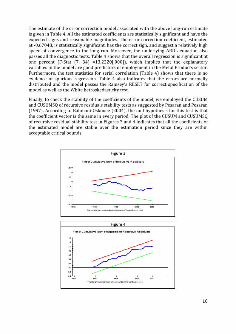
The estimate of the error correction model associated with the above long-‐run estimate is given in Table 4. All the estimated coefficients are statistically significant and have the expected signs and reasonable magnitudes. The error correction coefficient, estimated at -‐0.67048, is statistically significant, has the correct sign, and suggest a relatively high speed of convergence to the long run. Moreover, the underlying ARDL equation also passes all the diagnostic tests. Table 4 shows that the overall regression is significant at one percent (F-‐Stat (7, 34) =13.2220[.000]), which implies that the explanatory variables in the model are good predictors of employment in the Metal Products sector. Furthermore, the test statistics for serial correlation (Table 4) shows that there is no evidence of spurious regression. Table 4 also indicates that the errors are normally distributed and the model passes the Ramsey’s RESET for correct specification of the model as well as the White hetroskedasticity test.
Finally, to check the stability of the coefficients of the model, we employed the CUSUM and CUSUMSQ of recursive residuals stability tests as suggested by Pesaran and Pesaran (1997). According to Bahmani-‐Oskooee (2004), the null hypothesis for this test is that the coefficient vector is the same in every period. The plot of the CUSUM and CUSUMSQ of recursive residual stability test in Figures 3 and 4 indicates that all the coefficients of the estimated model are stable over the estimation period since they are within acceptable critical bounds.
Figure 3
-20
-10
0
10
20
1972 1983 1994 2005 2013
The straight lines represent critical bounds at 5% significance level
Plot of Cumulative Sum of Recursive Residuals
Figure 4
-0.4
-0.2
0.0
0.2
0.4
0.6
0.8
1.0
1.2
1.4
1972 1983 1994 2005 2013
The straight lines represent critical bounds at 5% significance level
Plot of Cumulative Sum of Squares of Recursive Residuals

19
Finally, we have used the generalized impulse response function (Koop et al. 1996; Pesaran and Shin 1998; and Potter 1998) to examine the responses of employment in the Metal Product sector to one standard deviation shock in independent variables in the ARDL equation for employment in the Metal Products sector. It captures how quickly the long-‐run relations in sector employment converge to their steady-‐state values. Figure 5 shows that near-‐complete adjustments are achieved after approximately (or less than) 10 years.
Figures 6 and 7 show the statistical tests of the estimated error correction model’s forecast performance conducted by splitting the data set into an in-‐sample period, used for the initial parameter estimation and model selection, and an out-‐of-‐sample period, used to evaluate forecasting performance. The root mean squares of forecast errors of around 0.67 percent per year compares favourably with the value of the same criterion computed over the estimation period.
The estimated ARDL equation for the Metal Product sector shows that employment in this sector is determined by several demand and supply factors. For example, ceteris paribus, a one percent increase in the sector real wage rate is expected to reduce sector employment by 0.6 percent. And, a one percent increase in the Gross Domestic Expenditure (GDE) is expected to lead to an increase in employment in the Metal Products sector of 0.16 percent in the short run and 0.24 percent in the long run. Moreover, a one percent increase in the real imports of Metal Products is expected to reduce the sector employment by 0.08 percent in the short run and 0.12 percent in the long run.
Figure 5
-0.04
-0.02
0.00
0.02
0.04
0.06
0 13 26 39 50
Generalised Impulse Responses to one SE shock in the equation for DLE447ME
DLE447ME DLRW494MP DLVA541MPDLFI353MP DLGDE11 DLRM635ME

20
Overall, the econometric estimation of MEMSA’s employment equations captures the short-‐ and long-‐term responsiveness of the sector’s demand for labour to various independent variables, including the real wage rate. Out of 40 estimated employment equations, employment in 36 sectors was found to have a statistically significant negative relationship with the sector real wage rate. The values of all the short-‐term wage elasticities are between minus one and zero. The estimated employment equation for the Rubber Product sector has the lowest estimated wage elasticity of -‐0.11028 and the Households sector has the largest wage elasticity of -‐0.84953. The wage elasticities of the remaining 34 sectors fall between the above two values. At the same time, the results show consistency between short-‐ and long-‐run wage elasticities within the sectors. This means that the sizes of the short-‐run elasticities are in line with the corresponding long-‐run elasticities, i.e. when the latter is relatively high in a sector, the short-‐run elasticity is likewise relatively high.
The above procedure was followed for the specification and estimation of the rest of the MEMSA equations associated with production, prices, labour market, trade sector, financial market, and others. The sectoral estimations were conducted for 40 sectors of the economy.
Figure 6
11.5
11.6
11.7
11.8
11.9
12.0
12.1
12.2
1972 1983 1994 2005 2013
Dynamic forecasts for the level of LE447ME
LE447ME Forecast
Figure 7
-0.2
-0.1
0.0
0.1
0.2
0.3
1972 1983 1994 2005 2013
Dynamic forecasts for the change in LE447ME
LE447ME Forecast
21
3.5. DIMMSIM’s microsimulation component The modelling principle employed to build the South African household model is the microsimulation modelling technique, whose application to socio-‐economic modelling was pioneered by Guy Orcutt in the United States in the late 50s and early 60s (Orcutt, 1957; Orcutt et al., 1961). The South African model, which was originally built as a static model (Adelzadeh, 2001), has been expanded and complemented with dynamic properties for the purpose of building DIMMSIM.
The main components of the model are its database and its tax and social policy modules that have been regularly updated and upgraded over the last 10 years. The South African model uses a micro-‐database of individuals and households comprising data from the official annual October Household Survey (1995 to 1999), the Income Expenditure Survey (1995 and 2000), the Census (1996, 2001 and 2011), Community Survey (2007), and the Quarterly Labour Force Survey, which are key sources of countrywide individual and household microdata. The model’s database is prepared in terms of family units, because it relates closely to the definition of the financial unit used by many of the government tax and transfer programmes. The model’s database includes 125 830 individuals, making up 61 684 families or 29 800 households. The database includes weights for individuals, families and households, which are used to translate each of the three samples to their corresponding populations for a given year. Each unit record includes more than 400 columns of information for each individual in the family – including demographic, labour force, marital status, housing, education, and income and expenditure information.
The data ageing is obtained by ‘reweighting’ and ‘uprating’ each record. Reweighting is used to modify the demographic, family and labour force characteristics of the model’s population. Uprating is used to update individual and family income and expenditure. CALMAR (caliberation of margins) is a reweighting algorithm that has been used to alter weights in a sample dataset to reflect a new population of reference. It applies given marginal totals to a set of initial weights on a survey record file. DIMMSIM endogenously uprates various categories of income and expenditure of individuals and families.
The South African microsimulation model includes three government taxation policies (i.e. personal income tax, excise tax, and value added tax), government’s expanded public work programme (EPWP), and six transfer programmes (i.e. old age grant, child support, disability grant, care dependency grant, care giver support, and the basic income grant). Four of the programs constitute government’s main social security programmes.
3.6. Accounting consistency within DIMMSIM Technically, two important distinguishing features of DIMMSIM relate to establishing two-‐way interactions between its underlying models and generating the model’s macro and household level results that embody the necessary accounting requirements for each period related to linked macro-‐micro models.

22
A considerable part of the model is concerned with enforcing the necessary accounting relationships both within and between the two models to ensure simulation results are consistent, meaningful and reliable. DIMMSIM’s iterative process of generating each period’s forecast ensures that the accepted simulation results for each period satisfies all the specified accounting relationships. For example, with regard to the macroeconomic model, the components of the product account add up, and the income and product sides of the accounts are equal. Moreover, the price/quantity relationships are consistent. Some of these relationships include:
• The income tax module of the microsimulation part of DIMMSIM estimates family-‐level income tax for each period, and feeds the information to the equation for the calculation of household disposable income, and the equation that captures sources of government current income, where the government’s overall revenue from taxes on income and wealth is made up of household and business enterprise contributions.
• Similarly, the VAT module of the microsimulation component of the DIMMSIM uses detailed household level expenditure to calculate the contribution of households to the government’s revenue from the VAT and excise taxes.
• The social security modules of the microsimulation model provide for the
estimation of households’ income from government’s direct transfers. For each year of the forecast, the model’s policy modules that capture the government’s current old age pension, child support, disability, care dependency, and war veteran grants, estimates the total number of eligible persons for each grant and the required budget allocation. Changes to the eligibility and entitlement conditions of either of these policies and changes in the overall poverty rate in the country (e.g. due to a rise in the unemployment rate) implies changes in the budgetary requirements of these programs. In turn, the estimated budgetary requirement of the above government programmes feed into the households’ income accounts and government’s expenditure account in the macroeconomic model.
3.7. Macro-‐micro interactions in DIMMSIM The model establishes two-‐way interactions between its macro and micro components such that (a) changes in macroeconomic variables (e.g., changes in prices, employment, and wage rates) influence welfare of individuals and families, and (b) changes in household level economic conditions (e.g., poverty, inequality, consumption, taxes, eligibility for social grant, etc.) influence macroeconomic outcomes. The Gauss-‐Seidel’s iterative method is used to solve the overall system. The procedure runs the two models for a number of interactions, allowing interactions between the macro and micro parts of the model, before it converges and generates the final results for each year of the forecast period. This ensures that each period’s results reflect convergence of the macroeconomic variables and household level variables at the aggregate level. Therefore, the two models are dynamically integrated and generate time-‐based results that reflect the actual process of policymaking and evaluation. Later on, the above

23
interaction between the macro and micro parts of the model helps explain how a national minimum wage ultimately affects households.
4. National minimum wage scenarios This section provides a basic description of five economic scenarios that were developed for this project. With the exception of the base (‘Business-‐As-‐Usual) scenario, which we specified to capture the current status quo without a NMW, the other four NMW scenarios were developed by the National Minimum Wage Research Initiative in CSID, at the University of Witwatersrand. These represent four distinct possible NMW policy choices, emanating from the scope of the policy debate. The aim of this project is neither to provide an exhaustive list of possibilities for the NMW in South Africa nor to establish a specific NMW for the country. ADRS’ mandate was to examine the potential impact of four scenarios, using a modelling approach that could take account of the direct, indirect and dynamic impacts of the NMW policy within the South African economy.
4.1. Base or “Business-‐as-‐Usual” scenario
The Base scenario, which is referred to as the Business-‐As-‐Usual (BAU) scenario, captures the economy ‘as it is’ currently, with no NMW. It posits what if economic performance continues its current path over the next 10 years, with the average real growth rate and the unemployment rate hovering around 2 percent and 24 percent, respectively. In order to isolate the impact of a NMW policy, this scenario establishes an overall economic policy outlook for the country that is assumed to remain unchanged with or without a NMW policy. The BAU scenario reflects a combination of the status quo in domestic economic policy and a relatively low-‐growth path for the rest of the world, especially among the OECD countries.
Key features of the Base scenario:
§ Fiscal Policy: The scenario captures the Treasury’s concern about the potential increase in the Debt-‐to-‐GDP ratio.23 It therefore sets low annual targets for the deficit-‐to-‐GDP ratio as a mechanism the Treasury will use to gradually bring down the debt-‐to-‐GDP ratio. In the model, as in practice, this implies closely aligning government expenditure with government revenue. Therefore, the scenario strives for achieving a balanced or close to balanced annual budget.
§ Monetary Policy: The scenario adheres to government’s current inflation-‐targeting policy and assumes that the policy will remain unchanged over the next 10 years. In the model, this means the interest rate varies in order to keep the inflation rate within the 3 to 6 percentage target band over time.
§ Public Investment: Nominal investment by general government and public corporations is designed to annually increase by 6 percent in order to keep pace with inflation.
23 MacLeod (2015).

24
§ Government Final Consumption (GFC) Expenditure: GFC is expected to grow by 6.2 percent annually in nominal terms, which closely corresponds to the MTEF’s average annual rate.
§ International Outlook: The scenario assumes that average real annual growth rate for the OECD and Sub-‐Saharan countries will be 1 percent and 5 percent respectively, over the next 10 years. The price of a barrel of crude oil is set to gradually increase to 70 US Dollars by 2025.
§ Taxes, Social Grants and EPWP: The scenario assumes that all nominal parameters related to direct and indirect taxes, social grants and EPWP (e.g., tax brackets, grant amounts) annually increase by 6 percent to keep up with inflation during the projection period.
§ Poverty Line: The scenario adopts a poverty line of R720 per capita and R930 per adult equivalent per month for 2015. Both poverty lines are adjusted by 6 percent annually.
4.2. NMW scenario 1: the ‘Minimal’ scenario This scenario examines what occurs if a relatively low NMW is added to the economy’s BAU scenario. It is referred to as a ‘Minimal’ scenario because it sets the NMW at a level close to the lowest sectoral determination for 2015, which amounts to R2 250 per month for full-‐time workers in 2016. The NMW is designed to annually adjust for inflation over the next 10 years.24
4.3. NMW scenario 2: the ‘Index 40%’ scenario This is one of two scenarios that examine what if a NMW is added to the BAU scenario using the wage indexation approach, as is used internationally.25 Indexing the minimum wage to the mean or median wage would automatically increase the minimum wage to keep pace with the typical worker’s wage while linking it to overall conditions in the labour market. In this way, minimum wage earners experience annual wage gains in line with overall demand for labour in the market. Moreover, wage indexing improves the ability of the national minimum wage policy to reduce inequality by ensuring that minimum wage earners do not increasingly fall behind the typical worker, thereby preventing widening disparities between the lowest paid and other workers.26
24 For the processing of the scenarios, the NMW module of DIMMSIM (Section 5) includes steps that ensure that only the wage rate of full-‐time workers in each sector of the economy is allowed to directly adjust to the NMW. See Finn 2015 for a methodological discussion on the issue of the NMW and full-‐time and part-‐time workers. 25 Castel-‐Branco (2016), and Konopelko (2015). 26 From ILO (2014:127-‐128, footnotes removed): “Several member States expressly establish a link between the minimum wage and the mean wage. For example, in Azerbaijan, measures have to be taken to gradually raise the minimum wage to the minimum subsistence level and 60 per cent of the mean wage. The minimum wage cannot be less than one third of the mean wage in Belarus, or below 55 per cent of the minimum wage in Bosnia and Herzegovina (Federation of Bosnia and Herzegovina). In the former Yugoslav Republic of Macedonia, the minimum wage corresponds to 39.6 per cent of the average wage, as established by the State Statistical Office for the preceding year. In France, the annual increase in

25
For ease of reference, we refer to this scenario as the NMW ‘Index 40%’.
Key features:
§ In 2016, the NMW is indexed to 40 percent of the inflation-‐adjusted average real wage rate for all full-‐time workers in 2015, or R3 467.
§ The index is increased annually by 1 percent until it reaches 45 percent of the inflation-‐adjusted 2015 mean real wage rate. After 2021, the index will remain at 45 percent.
§ For three very low-‐wage sectors different rates are set as a percentage of the NMW for each year. For agriculture, the rate is set to 80 percent of the NMW. For domestic workers and the EPWP workers, the rate is set at 70 percent of the NMW.27
4.4. NMW scenario 3: the Index 45% scenario This scenario adopts a similar approach to Scenario 2. However, by setting the index to 45 percent of the mean real wage rate of full-‐time formal workers, it seeks to use the NMW policy to improve the living standards of a larger portion of workers. Based on the Labour Force Survey of 2014, it is expected to impact 55 to 60 percent of full-‐time workers.
Key features:
§ In 2016, the NMW is indexed to 45 percent of the inflation-‐adjusted average real wage rate for full-‐time formal sector workers in 2015, excluding agriculture and domestic work, or R4 623.
§ The index increases annually by 1 percent until it reaches 50 percent of the inflation-‐adjusted 2015 mean real wage rate. After 2021, the index will remain at 50 percent.
§ For the agriculture sector, the rate is set to 80 percent of the NMW, while for domestic workers and the EPWP the rate is set at 70 percent of the NMW.
the purchasing power of the SMIC cannot be less than half the increase in the purchasing power of the average hourly wages recorded by the quarterly survey of the Ministry of Labour. In Israel, according to the Government, the minimum wage is fixed at 47.5 per cent of the mean wage. In Montenegro, the minimum wage cannot be less than 30 per cent of the mean wage for the preceding six months, as established by the Statistical Office. In the Netherlands, the minimum wage is indexed to the average rate of wage increases in the public and private sectors, as calculated by the Netherlands Bureau for Economic Policy Analysis (CPB). In Poland, according to the Government’s report, the increase in the minimum wage, which cannot be less than that of the forecast CPI, is increased by two-‐thirds of the forecast growth in GDP when the minimum wage is less than half the mean wage. The mean wage is also taken into account in fixing minimum wages in the Republic of Moldova, Serbia, Slovakia, Ukraine, and some provinces of Canada, as well as in Hungary, New Zealand and the United Kingdom, according to their Governments’ reports.” 27 The basis for these ‘tiers’ is discussed in detail in Konopelko (2015) and Castel-‐Branco (2016).

26
4.5. NMW scenario 4: the ‘Maximal’ scenario
This scenario examines what occurs if a relatively high NMW is added to the economy’s BAU scenario. The scenario is referred to as the ‘Maximal’ scenario because it tests the impact of an aggressive NMW policy to possibly transform South Africa’s wage structure significantly.
Key features:
§ The NMW begins in 2016 at R6 000 per month for full-‐time workers.
§ It adjusts annually for inflation plus 2 percent until 2021. After 2021, the NMW is expected to annually adjust to inflation.
§ The minimum wage for three very low-‐wage sectors is set as a percentage of the national minimum wage each year. For agriculture, the rate is set to 80 percent of the NMW. For domestic work the rate is pegged at 70 percent of the NMW. For EPWP workers, the rate is set at 60 percent of the NMW.
Figures 8 and 9 present the evolution of the NMW under the above four scenarios over the next 10 years. They show that after 2016, nominal NMW rates increase between 6 percent and 7.4 percent average annually, and real NMW rates increase between zero percent and 1.32 percent, average annually.28
5. National minimum wage module For the purpose of this research, a new module was added to DIMMSIM to facilitate the design and simulation of various formulations of the NMW for South Africa. The module’s computer codes capture the features of the NMW scenarios, and estimate and transmit the magnitudes of annual shocks to the 45 sector average real wage equations of DIMMSIM. The module is designed to accommodate variations of a given NMW, such as temporary or permanent sectoral exemptions, annual adjustments to the NMW, and the introduction of NMW as a flat rate or in indexed form. Finally, in the microsimulation component of DIMMSIM, the module is responsible for adjusting the wage income of existing full-‐time workers whose current wage rates are below the scenario’s NMW rate.
28 Between 2016 and 2021, nominal NMW rates increase between 6 percent and 8.5 percent average annually, and real NMW rates increase between zero percent and 2.38 percent average annually
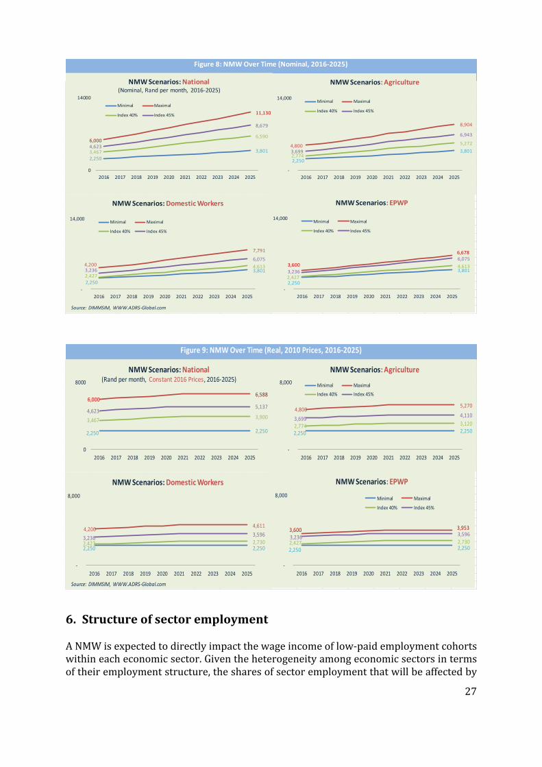
27
6. Structure of sector employment A NMW is expected to directly impact the wage income of low-‐paid employment cohorts within each economic sector. Given the heterogeneity among economic sectors in terms of their employment structure, the shares of sector employment that will be affected by
Figure 8: NMW Over Time (Nominal, 2016-‐2025)
2,250 3,801
6,000
11,130
3,467
6,590
4,623
8,679
0
14000
2016 2017 2018 2019 2020 2021 2022 2023 2024 2025
NMW Scenarios: National(Nominal, Rand per month, 2016-‐2025)
Minimal Maximal
Index 40% Index 45%
2,250
3,801 4,800
8,904
2,774
5,272 3,699
6,943
-‐
14,000
2016 2017 2018 2019 2020 2021 2022 2023 2024 2025
NMW Scenarios: Agriculture
Minimal Maximal
Index 40% Index 45%
2,250
3,801 4,200
7,791
2,427
4,613 3,236
6,075
-‐
14,000
2016 2017 2018 2019 2020 2021 2022 2023 2024 2025
Source: DIMMSIM, WWW.ADRS-‐Global.com
NMW Scenarios: Domestic Workers
Minimal Maximal
Index 40% Index 45%
2,250
3,801 3,600
6,678
2,427
4,613 3,236
6,075
-‐
14,000
2016 2017 2018 2019 2020 2021 2022 2023 2024 2025
NMW Scenarios: EPWP
Minimal Maximal
Index 40% Index 45%
Figure 9: NMW Over Time (Real, 2010 Prices, 2016-‐2025)
2,250 2,250
6,000 6,588
3,467 3,900 4,623
5,137
0
8000
2016 2017 2018 2019 2020 2021 2022 2023 2024 2025
NMW Scenarios: National(Rand per month, Constant 2016 Prices, 2016-‐2025)
2,250 2,250
4,800 5,270
2,774 3,120 3,699 4,110
-‐
8,000
2016 2017 2018 2019 2020 2021 2022 2023 2024 2025
NMW Scenarios: Agriculture
Minimal Maximal
Index 40% Index 45%
2,250 2,250
4,200 4,611
2,427 2,730 3,236 3,596
-‐
8,000
2016 2017 2018 2019 2020 2021 2022 2023 2024 2025
Source: DIMMSIM, WWW.ADRS-‐Global.com
NMW Scenarios: Domestic Workers
2,250 2,250
3,600 3,953
2,427 2,730 3,236 3,596
-‐
8,000
2016 2017 2018 2019 2020 2021 2022 2023 2024 2025
NMW Scenarios: EPWP
Minimal Maximal
Index 40% Index 45%

28
the NMW differ. DIMMSIM’s sector employment time series database does not include the employment structure within each sector. Arden Finn, commissioned by the NMW Research Initiative, used the Labour Market Dynamics in South Africa 2014 (LMDSA 2014) dataset to calculate the share of full-‐time workers in total employment of each sector and to break down DIMMSIM’s sector employment into 8 cohorts, each with its own average wage income. Table 5 shows the share of full-‐time workers employed in each sector, the share of the eight cohorts in full-‐time employment in each sector, and the corresponding average wage incomes. As expected, the table shows significant variation in economic sectors in terms of the share of low-‐wage full-‐time workers in total full-‐time employment within the sectors. For example, the wage income of 64 percent of full-‐time workers in the Agriculture sector was below R2 250 a month in 201, compared to the zero percent share of employment in the “Motor vehicles, parts and accessories” sector. On average, the wage income of 25.2 percent of full-‐time workers of all economic sectors was below R2 250 a month. However, a high standard deviation of 12.9 reflects a large variation among sectors. Overall, the monthly wage incomes of 2.93 million out of 10.2 million full-‐time workers, i.e., 28.8 percent, were below R2 250 in 2014, with about three-‐fourths (73.4 percent) working in the service sector, 14.3 percent in the primary sector and 12.3 percent in the manufacturing sector.
For the simulation of the NMW scenarios, it is assumed that the share of full-‐time workers in total sector employment and the eight employment shares within each sector will not change over the forecast period.29 The model uses the annual NMW value related to a given scenario to replace the average wage rates of employment cohorts whose rates are below the relevant NMW for that period. This provides the basis for estimating the magnitudes of shocks to the sector average real wage rates as a result of introducing a NMW. After the initial year, the model takes account of previous year’s adjustments of wage rates of low-‐paid cohorts in each sector and only adjusts particular cohorts’ average wage rates, if the NMW scenario requires.
29 The justification for this assumption is that the composition of employment, by occupations or skills, in a given sector remains relatively stable over time.

29
7. Analysis of results In preparing to run simulations of the NMW scenarios, various data sets of DIMMSIM were fully updated using the latest available Reserve Bank and Statistics South Africa data.30 In this section of the report, analysis of the potential impact of the NMW over the next ten years (2016-‐2025) is centred on aspects of the model’s dynamics that are relevant for understanding how the NMW policy ultimately influences the economy and households. The section is divided into nine headings. Sections 7.1 and 7.2 compare 30 Both macro and micro model components of DIMMSIM are annually updated. The macro model database is updated using South African Reserve Bank time-‐series data and Quantec’s industry time-‐series data. The values of the model’s exogenous variables are also updated using various data sources. The microsimulation model’s demographic and income and expenditure data sets are also annually aged and uprated. Therefore, DIMMSIM always runs with the latest available annual data. This is different from the CGE models that are calibrated for a benchmark year and do not reflect latest macro and micro data. For example, the model used by the Treasury Department is calibrated for 2009 and the model used by Pauw and Leibbrandt (2012) is calibrated for 2000 data.
Share (%) Mean Income Share Mean Share Mean Share Mean Share Mean Share Mean Share Mean Share Mean1 Agriculture, Forestry and Fishing 92.7 9.2 R507 9.1 R1,066 9.8 R1,481 35.9 R2,125 20.3 R2,637 7.6 R3,750 2.3 R5,380 5.7 R22,2452 Coal Mining 97.6 13.1 R1,235 13.9 R3,691 8.8 R4,834 14.3 R6,386 13.7 R8,898 9.3 R14,258 17.5 R18,511 9.5 R31,4203 Gold, uranium and ore mining 95.4 16.3 R1,220 9.7 R3,180 5.4 R4,307 17.0 R5,900 23.7 R7,985 12.0 R11,251 7.5 R15,735 8.4 R39,8444 Other mining 82.0 13.5 R1,568 8.5 R3,525 7.9 R5,217 14.7 R6,469 20.2 R8,400 21.9 R11,765 5.8 R16,562 7.5 R46,9135 Food 94.5 17.8 R782 12.1 R2,047 10.9 R2,753 21.4 R3,504 11.4 R5,148 10.0 R6,996 3.4 R10,463 12.9 R23,2196 Beverages 94.6 32.0 R1,755 14.0 R4,279 10.5 R5,884 14.7 R8,269 9.6 R11,000 2.7 R15,855 7.1 R22,379 9.4 R79,2567 Tobacco 98.6 17.8 R782 12.1 R2,047 10.9 R2,753 21.4 R3,504 11.4 R5,148 10.0 R6,996 3.4 R10,463 12.9 R23,2198 Textiles 93.7 40.1 R2,581 19.9 R2,846 7.0 R4,497 14.3 R5,994 2.0 R7,137 5.3 R11,639 2.1 R22,650 9.4 R99,5279 Wearing Apparel 95.9 15.5 R631 23.0 R1,628 11.7 R2,204 22.2 R3,080 8.0 R4,135 5.7 R6,056 3.4 R8,040 10.5 R25,74310 Leather and Leather products 90.8 8.3 R347 1.4 R1,248 8.7 R1,907 24.9 R2,306 31.1 R3,728 11.9 R4,535 6.2 R7,951 7.4 R18,29011 Footwear 90.8 8.3 R347 1.4 R1,248 8.7 R1,907 24.9 R2,306 31.1 R3,728 11.9 R4,535 6.2 R7,951 7.4 R18,29012 Wood and wood products 97.5 25.4 R1,611 18.9 R2,960 7.3 R3,915 16.8 R3,561 10.7 R4,944 11.3 R5,421 2.1 R13,968 7.5 R57,68013 Paper and paper products 97.3 20.8 R436 7.3 R2,102 7.8 R3,081 18.7 R3,912 17.1 R5,651 5.6 R7,983 10.9 R11,374 11.8 R24,26714 Printing, publishing and recorded media 93.7 27.5 R924 9.7 R2,339 7.8 R3,161 9.7 R4,221 8.0 R6,072 12.2 R8,524 11.6 R12,144 13.5 R24,26715 Coke and refined petroleum products 95.5 26.4 R1,656 8.6 R4,532 5.1 R6,316 7.3 R8,723 6.2 R12,947 26.2 R16,261 10.6 R23,558 9.6 R54,97216 Basic chemicals 95.0 28.9 R564 3.2 R2,379 8.2 R3,080 20.8 R4,121 3.6 R5,748 15.7 R7,622 1.3 R12,481 18.3 R21,00317 Other chemicals and man made fibres 94.3 20.7 R1,175 17.7 R3,186 4.7 R4,344 17.3 R5,882 7.1 R8,311 14.1 R12,375 4.6 R17,431 13.8 R35,36918 Rubber products 92.1 12.9 R706 3.7 R2,467 0.0 R0 25.5 R4,716 19.8 R6,196 22.2 R8,897 6.2 R12,541 9.7 R18,69519 Plastic products 98.4 18.1 R841 12.3 R2,288 6.0 R3,144 25.8 R4,043 15.4 R5,812 9.6 R8,665 3.3 R12,129 9.4 R34,18320 Glass and glass products 98.4 17.9 R915 13.6 R2,760 7.6 R3,468 26.7 R4,649 4.3 R6,827 4.4 R8,848 4.1 R12,312 21.5 R22,29321 Non-‐metalic minerals 96.0 24.6 R845 22.6 R1,952 9.6 R2,642 10.5 R3,544 6.9 R5,190 7.6 R7,135 4.7 R10,393 13.5 R24,36222 Basic iron and steel 96.7 17.1 R1,332 19.0 R3,689 11.2 R5,158 15.9 R6,535 9.9 R9,434 9.2 R13,768 9.6 R19,300 8.1 R54,52523 Basic non-‐ferrous metals 95.6 18.8 R1,392 15.9 R3,910 8.1 R5,806 17.9 R6,762 9.8 R10,442 3.6 R14,893 5.4 R20,268 20.6 R33,49224 Metal products excluding machinery 95.4 15.6 R1,029 13.4 R2,382 14.6 R3,543 18.5 R4,746 8.6 R6,366 14.2 R8,713 4.3 R12,818 10.8 R33,80025 Machinery and equipment 96.1 20.7 R1,156 6.7 R3,410 9.9 R4,369 20.7 R5,053 6.8 R7,628 16.7 R10,939 3.8 R16,802 14.8 R28,40226 Electrical equipment 89.5 20.7 R1,156 6.7 R3,410 9.9 R4,369 20.7 R5,053 6.8 R7,628 16.7 R10,939 3.8 R16,802 14.8 R28,40227 Television, radio and communication equipment 100.0 14.4 R834 9.0 R2,995 17.3 R4,069 10.4 R4,899 16.9 R7,300 13.3 R11,128 5.6 R16,130 13.0 R28,72628 Professional & scientific equipment 93.5 14.4 R834 9.0 R2,995 17.3 R4,069 10.4 R4,899 16.9 R7,300 13.3 R11,128 5.6 R16,130 13.0 R28,72629 Motor vehicles, parts & accessories 97.1 33.7 R2,798 13.9 R7,818 10.3 R7,681 13.6 R10,546 5.0 R10,380 7.7 R16,579 5.9 R31,231 9.8 R134,81230 Other transport equipment 86.0 33.7 R2,798 13.9 R7,818 10.3 R7,681 13.6 R10,546 5.0 R10,380 7.7 R16,579 5.9 R31,231 9.8 R134,81231 Furniture 96.9 17.6 R981 23.9 R1,927 15.6 R2,730 14.3 R3,868 6.7 R5,459 5.8 R6,604 1.6 R10,909 14.5 R25,14732 Other manufacturing 93.2 9.7 R772 9.6 R1,619 18.2 R2,372 30.4 R3,225 10.2 R4,363 7.3 R5,946 4.4 R8,000 10.2 R20,21633 Electricity, Gas and water 93.1 24.4 R1,703 13.3 R4,128 7.3 R5,943 14.4 R8,269 11.0 R11,828 12.6 R17,421 8.4 R22,886 8.6 R64,89434 Building construction and engineering 85.1 18.5 R991 19.0 R2,146 16.0 R2,991 19.0 R4,072 7.9 R5,820 8.0 R8,206 3.0 R11,654 8.7 R39,13435 Wholesale, retail trade, catering and accomodation services 91.6 20.7 R1,164 22.1 R2,561 10.2 R3,318 17.9 R4,195 7.6 R5,994 6.6 R9,018 4.6 R12,993 10.3 R39,09036 Transport, storage, and communication 93.3 19.6 R1,120 14.4 R2,478 9.1 R3,741 16.2 R4,556 9.2 R6,732 14.9 R10,835 5.3 R15,386 11.4 R32,06237 Financial services, business intermediation, insurance & real estate 92.9 19.0 R1,714 14.2 R3,475 11.3 R3,660 19.6 R5,337 9.3 R9,674 10.9 R13,867 5.5 R19,520 10.1 R49,86338 Community, social & personal services 76.6 23.1 R1,224 10.7 R2,118 7.7 R3,034 14.9 R3,912 12.2 R5,693 15.9 R8,727 8.2 R15,055 7.2 R41,13839 Other services 80.4 28.7 R1,379 13.1 R3,215 7.9 R4,100 14.0 R5,544 8.5 R9,085 11.9 R13,277 6.8 R17,336 9.1 R49,91840 Other producers 57.7 6.0 R354 8.6 R749 11.1 R1,005 24.6 R1,407 21.7 R1,950 18.9 R2,670 5.5 R3,752 3.7 R14,82441 General government services 87.5 27.3 R1,466 10.1 R4,190 5.8 R5,704 10.9 R8,521 10.3 R11,269 17.4 R15,259 10.7 R20,662 7.4 R60,33842 Total Primary 91.4 16.6 R826 24.0 R1,940 17.2 R2,515 10.0 R3,485 5.6 R5,076 10.9 R7,371 5.7 R9,899 10.0 R27,77043 Total manufacturing 95.3 26.7 R1,204 17.0 R2,911 10.9 R4,056 14.9 R5,673 6.6 R7,834 8.1 R11,301 4.9 R16,141 10.9 R43,48944 Total services 84.8 28.6 R1,253 19.0 R2,814 9.0 R3,931 10.5 R5,376 6.4 R7,721 8.2 R10,919 7.2 R15,560 11.0 R41,84845 Total economy 86.6 28.1 R1,232 19.8 R2,750 8.7 R3,889 11.1 R5,319 6.7 R7,592 8.2 R10,748 6.0 R15,244 11.3 R40,207
Source: Authors' preparation based on A. Finn (2015). Data Source: Labour Market Dynamics in South Africa 2014.
[75%; 100%) [100%; 150%) [150%; 200] >200%Full Employment Share (%)
Table 5: Sector Employment Cohorts with Monthly Mean IncomeADRS Sector Codes
<25% [25%; 40%) [40%; 50%) [50%; 75%)

30
scenarios in terms of the magnitudes of shocks to sector wage rates due to the introduction of the NMW and the model results for sector wage rates under the five NMW scenarios over the forecast period. Section 7.3 analyses the impact of the NMW scenarios on household income. The focus of Section 7.4 is on the effects of the NMW on household consumption expenditure. Section 7.5 presents model results for GDP and sector outputs. The employment impact of the NMW scenarios is presented in Section 7.6, followed by a comparison of scenarios in terms of their impact on other key macroeconomic indicators, such as labour productivity (Section 7.7), and the inflation rate (Section 7.8). Section 7.9 is dedicated to the impact of the NMW scenarios on poverty and inequality indicators, and Section 7.10 provides an overall comparison of performances of the scenario results.
7.1. National minimum wage and sector shocks As explained in Section 3.1, DIMMSIM’s industry structure includes 45 estimated equations for the average real wage rates and 45 equations for the average nominal wage rates.31 The introduction of a NMW in 2016 is expected to impact sector nominal and real average wage rates. The magnitude of the first year shock (i.e., 2016) to a sector’s average wage rate is calculated based on the employment share of cohorts with average wage rates below the NMW for the sector and the differences between the NMW for the sector and the average wage rates of the same employment cohorts.
DIMMSIM’s estimate of the initial (first year) shock to the economy-‐wide average real wage rate ranges from 0.32 percent (Minimal scenario), 0.76 percent (Index 40% scenario), 1.57 percent (Index 45% scenario), and 2.54 percent (Maximal scenario). At sector level, the average magnitudes of the initial shocks to the sector real wage rates range from 0.27 percent (Minimal scenario) to 2.16 percent (Maximal scenario). The list of sectors whose average wage rates will be most (or least) affected vary slightly across the NMW scenarios, since the distribution of low-‐wage workers across sectors and across wage bands within sectors differ, see Table 6. Therefore, under the Minimal Scenario, the top four sectors with the highest initial (first year) shocks to their average real wage rates include the household sector, basic chemicals, non-‐metallic minerals and wearing apparel. Under the Maximal Scenario, the top four sectors with the highest shocks to their average real wage rates change to wearing apparel, non-‐metallic minerals, furniture and footwear.
Under both the Minimal and Index 40% Scenarios, the average real wage rates for the primary, manufacturing and services sectors are expected to increase by less than one percent, with relatively higher percentage changes for the Index 40% Scenario. Under the Index 45% Scenario, the introduction of the NMW is estimated to increase the average real wage rates for the primary, manufacturing, and services sectors by between 1.43 percent and 1.98 percent. The corresponding increases under the Maximal Scenario are expected to range between 2.34 percent and 3.1 percent.
31 In DIMMSIM, the 45 sectoral nominal wage rates are calculated as the product of the 45 estimated average real wage rate and 45 estimated sector prices.

31
Minimal Index 40 Index 45 MaximalAgric, Forestry and Fishing 0.44 0.70 1.73 2.86Coal Mining 0.15 0.30 0.65 1.18Gold, uranium and ore mining 0.19 0.39 0.80 1.31Other mining 0.10 0.26 0.57 0.98Food 0.32 0.73 1.63 2.71Beverage 0.18 0.55 1.09 1.82Tobacco 0.32 0.73 1.63 2.71Textiles 0.17 0.41 1.34 2.38Wearing Apparel 0.45 1.08 2.23 3.49Leather and Leather products 0.23 0.71 1.71 3.05Footwear 0.23 0.71 1.71 3.05Wood and wood products 0.18 0.54 1.48 2.75Paper and paper products 0.44 0.78 1.48 2.40Printing, publishing and recorded media 0.41 0.84 1.58 2.43Coke & refined petroleum products 0.18 0.48 0.90 1.44Basic chemicals 0.55 0.93 1.67 2.63Other chemicals & man made fibres 0.25 0.51 1.11 1.80Rubber products 0.23 0.41 0.66 1.29Plastic products 0.29 0.64 1.37 2.37Glass and glass products 0.27 0.55 1.14 2.15Non-metalic minerals 0.47 1.08 2.08 3.19Basic iron & steel 0.18 0.37 0.84 1.51Basic non-ferrous metals 0.18 0.40 0.81 1.37Metal products excl.machinery 0.22 0.53 1.15 2.09Machinery and equipment 0.26 0.50 0.93 1.74Electrical equipment 0.26 0.50 0.93 1.74Tv, radio & communication equipment 0.23 0.42 0.89 1.65Professional & scientific equipment 0.23 0.42 0.89 1.65Motor vehicles, parts & accessories 0.00 0.18 0.70 1.22Other transport equipment 0.00 0.18 0.70 1.22Furniture 0.34 0.91 1.91 3.07Other industries 0.23 0.65 1.72 2.94Electricity, Gas and water 0.15 0.43 0.88 1.48Building construction and engineering 0.29 0.77 1.71 2.85Wholesale, retail trade, catering and accomodation services 0.25 0.67 1.56 2.67Transport, storage, and communication 0.25 0.60 1.23 2.15Financial services, business intermediation, insurance & real estate0.12 0.33 0.93 1.77Other services 0.28 0.62 1.31 2.16Households 0.74 0.69 1.63 2.68General government 0.24 0.25 0.44 0.45Total Primary 0.35 0.96 1.98 3.09Total manufacturing 0.32 0.69 1.43 2.34Total services 0.32 0.75 1.55 2.51Total economy 0.32 0.76 1.57 2.54
Maximum 0.74 1.08 2.23 3.49Minimum 0.00 0.18 0.44 0.45Average 0.27 0.59 1.28 2.16
Standard Deviation 0.13 0.22 0.45 0.71Source: ADRS Dynamically Integrated Macro-‐Micro Simulation Model (DIMMSIM)
Table 6: Initial Shocks to Sector Average Real Wage Rates (2016, %)
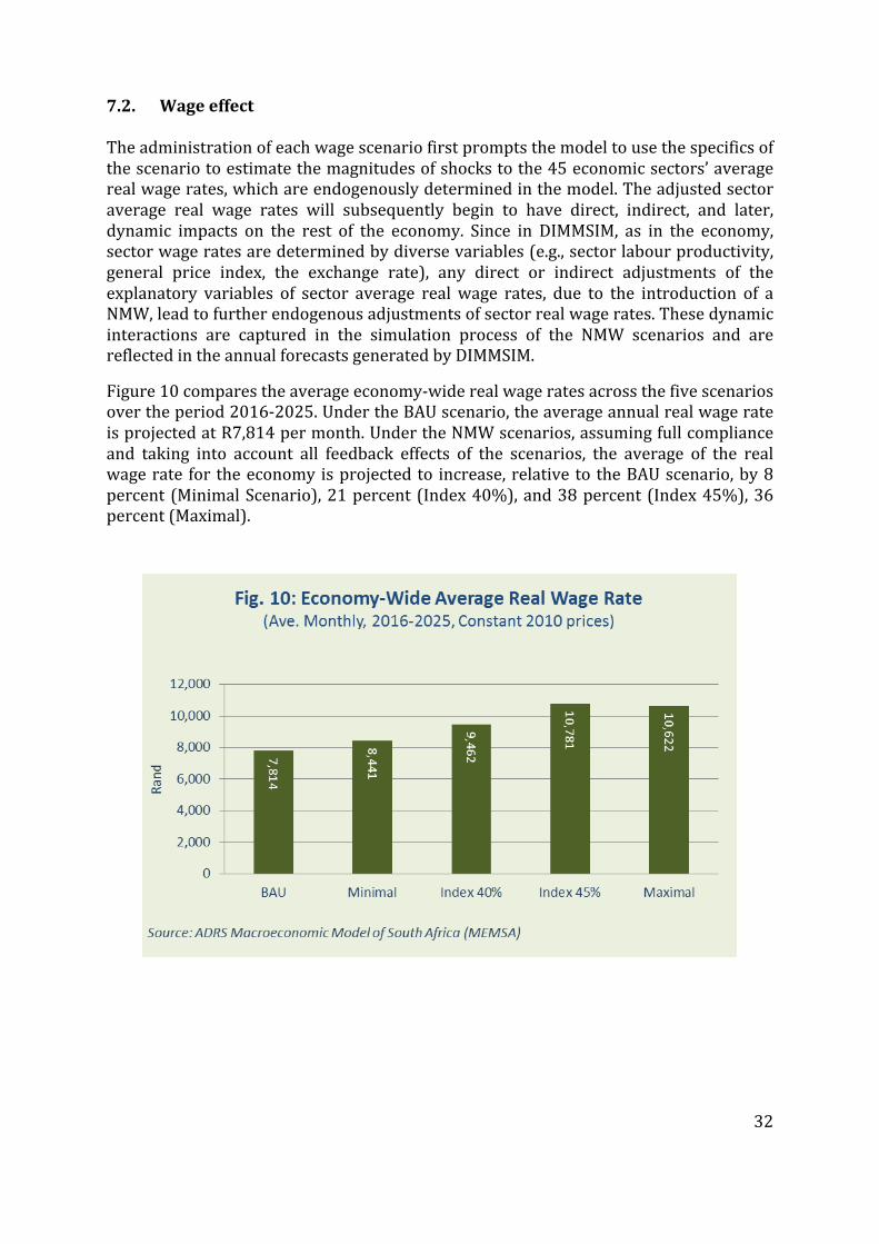
32
7.2. Wage effect The administration of each wage scenario first prompts the model to use the specifics of the scenario to estimate the magnitudes of shocks to the 45 economic sectors’ average real wage rates, which are endogenously determined in the model. The adjusted sector average real wage rates will subsequently begin to have direct, indirect, and later, dynamic impacts on the rest of the economy. Since in DIMMSIM, as in the economy, sector wage rates are determined by diverse variables (e.g., sector labour productivity, general price index, the exchange rate), any direct or indirect adjustments of the explanatory variables of sector average real wage rates, due to the introduction of a NMW, lead to further endogenous adjustments of sector real wage rates. These dynamic interactions are captured in the simulation process of the NMW scenarios and are reflected in the annual forecasts generated by DIMMSIM.
Figure 10 compares the average economy-‐wide real wage rates across the five scenarios over the period 2016-‐2025. Under the BAU scenario, the average annual real wage rate is projected at R7,814 per month. Under the NMW scenarios, assuming full compliance and taking into account all feedback effects of the scenarios, the average of the real wage rate for the economy is projected to increase, relative to the BAU scenario, by 8 percent (Minimal Scenario), 21 percent (Index 40%), and 38 percent (Index 45%), 36 percent (Maximal).

33
Under the NMW scenarios, the average annual increase in the primary sector’s mean real wage rate is projected to increase from 2.7 percent under the BAU scenario to 4 percent (Minimal), 5.9 percent (Maximal), 6.9 percent (Index 40%) and 5.7 percent (Index 45%).
The service sector employed 78 percent (about 7.95 million) of all full-‐time workers in 2014, which included about 3.8 million workers (47.6 percent) that earned less than R2 815 a month.32 The average wage rate in the sector will therefore be significantly affected by the introduction of a NMW. Relative to the BAU scenario, the average annual increase in the service sector’s mean real wage rate is projected to be higher by between 2.6 percent (Minimal) and 10.9 percent (Maximal).
Relative to the primary and service sectors, manufacturing has a smaller portion of full-‐time workers that earn wage rates below the NMW scenarios. Therefore, the average wage rate in the manufacturing sector will be less directly affected by the introduction of the NMW. Only under the Maximal NMW scenario, which covers a large portion of full-‐time workers, will the average annual real wage rate in manufacturing be significantly higher (Figure 11).33
Our findings that the introduction of a NMW in South Africa will especially increase wages at the bottom of the distribution, mainly in the primary and service sectors, are supported by similar findings of Lee (1999), Autor et al. (2015), and Dube et al.(2010). Our general finding that a NMW will positively impact the economy-‐wide average wages in South Africa through its effect on the wage distribution is also in line with findings from DiNardo et al.(1996), Lee (1999), Harris and Kearney (2014). According to
32 Based on Finn (2015) calculations using theLabour Market Dynamics in South Africa 2014. 33 Dube et al. (2010) reach similar conclusion with respect to the effect of minimum wages changes on manufacturing wages.
2.7
2.3
0.5
1.3
4.0 2.4
3.1 2.5
5.9
2.4
6.4
4.1
6.9
2.4
7.9
5.6
5.7 4.3
11.4
8.5
0
2
4
6
8
10
12
14
Primary Manufacturing Services Total economy
( % )
Source: DIMMSIM, www.ADRS-‐Global.com
Fig. 11: NMW and Real Wage Rate Growth(Avg. annual growth rate, 2016-‐2025)
BAU Minial Index 40 Index 45 Maximal

34
Cunningham (2007), in Latin America, a 10 percent increase in minimum wages results an increase in average wages of between 1 and 6 percent.
Overall, the introduction of the NMW and the subsequent wage adjustments of more than 4 million full-‐time workers across sectors of the economy help increase the average sector wage rates from below. This contrasts with historical trends of increases in sector average wage rates resulting from disproportionate increases in the remuneration of high-‐level occupations and high skilled workers.
7.3. Household income effect
Figure 12 presents the model’s results for household income under the BAU and the four NMW scenarios. The results reflect the net effect of direct and indirect channels that short-‐ and long-‐term forces bring to bear on the evolution of household income under each scenario. They also reflect interactions between the macroeconomic and microsimulation parts of DIMMSIM.
The model results show that the implementation of a NMW will directly increase the wage income of millions of workers. The number of beneficiaries of the policy and the extent of the benefits over time depend on the evolution of the sector employment, the sector average wage rates, and the eight average wage rates within each sector. As stated earlier, with the NMW, at least 4.26 million (Minimal Scenario) workers are expected to benefit from the implementation of the policy. Since the negative impact of the NMW on employment, calculated as the difference between the average annual level of employment under the NMW scenarios and the BAU scenario, is projected to be relatively small, between 1 600 (minimal) and 43 000 (Index 45%),34 the overall number of workers that are projected to benefit from the policy far exceeds the relatively small number of workers that may lose their jobs as a result. This, in turn, is reflected in the model’s projection of significant increases in real household gross income under the NMW scenarios, which is fully in line with international studies. For example, the Alonso (2015) study of US data shows that the minimum wage has a significant and positive impact at the bottom of the labour-‐income distribution. He shows that a 10 percent increase in the minimum wage would raise labour income by 0.8 percent at the 10th percentile and by 0.6 percent at the 25th. The Dube et al. (2010), and Allegretto et al. (2011) studies of the effects of minimum wages on earnings in low-‐wage sectors find strong positive earning effects as a result of minimum wage increases.
34 See section 7.6.

35
With the BAU scenario, household real gross income is projected to increase by an average annual rate of 3.3 percent.35 Relative to the BAU scenario, implementation of the NMW over the next 10 years is projected to increase the rate of growth of household income by 0.16 percent (Minimal Scenario), 1.3 percent (Index 40%), 1.25 percent (Index 45%) and 3.3 percent (Maximal Scenario), Figure 12.
Importantly, the contribution of a NMW to the increase in household income mainly reflects its positive impact on the income of more than four million low-‐wage full-‐time workers36 (i.e., the bottom of the distribution) and much less on the increase in the income of higher earner population groups (i.e., the top of the distribution).37 This distinction between the BAU scenario and the NMW scenarios has significant implications for the evolution of poverty and inequality over the next 10 years, which will be discussed in Section 7.9.
7.4. Household consumption effect The boost to real household income that follows the introduction of the NMW will positively impact household expenditure (i.e., demand) on goods and services. DIMMSIM uses 27 equations to represent real household consumption expenditure. Twenty-‐two of these are time-‐series estimated equations that capture the expenditure behaviour of households related to 5 categories of durable goods, 5 categories of semi-‐durable goods, 6 categories of non-‐durable goods, and 6 categories of services. The remaining 5 equations aggregate the model’s relevant equations to generate
35 Over the period between 2004 and 2014, the real gross primary income of households increased at compound annual growth rate of 2.5 percent. 36 As stated earlier, the Minimal scenario is projected to benefit 4.26 million full-‐time workers during the first year of implementing the NMW policy. 37 To the extent that in DIMMSIM, total sector employment is a function of the average real remuneration rate in that sector, the positive impact of a NMW on the average real wage rates of economic sectors affect total estimated sector employment and remunerations.

36
households’ total expenditure and its breakdown between durable, semi-‐durable, non-‐durable, and services.
Figure 13 depicts trends in household real consumption expenditure under alternative NMW scenarios. It shows that even though the Minimal scenario is able to result in higher annual household consumption expenditure, the scenario does not significantly change the pace (slope) at which real household consumption expenditure grows over time. On the other hand, the projections of trends for the two index scenarios and the Maximal scenario show both higher levels and faster rates of growth of household consumption expenditure relative to the BAU and the Minimal scenarios.38
The model’s results also depict the longer-‐term dynamic effect of the NMW on household consumption expenditure. This is illustrated in Figure 13. It shows that even though the levels of various NMW are kept constant in real terms after 2021, relative to a 1.9 percent average annual growth rate of real household consumption under the BAU scenario during 2022-‐2025, the corresponding growth rates under the four NMW scenarios will be higher at 2.0 percent (Minimal), 2.68 percent (Index 40%), 2.63 percent (Index 45%) and 3.64 percent (Maximal). This reflects the positive impact of the NMW on the expected long-‐term household income, which is one of the determinants of the household annual consumption expenditure in DIMMSIM.39
38 Kantor (2015) has argued that: “The essential condition for any step up in growth rates is an increased willingness of households to spend and borrow more.” 39 The cointegration estimation technique that has been used in DIMMSIM captures the impact of the trend in household real disposable income on the annual projections of household real consumption expenditures. The permanent income hypothesis, Friedman (1957) and Sargent (1987), posits that the household consumption expenditure at a point in time is partly determined by the expected income in future years.

37
Figure 14 presents a comparison of scenarios in terms of the growth of total household consumption expenditure and its four aggregate categories. It shows that over the next 10 years, total household consumption expenditure (in 2010 prices) is projected to annually grow by an average rate of 2 percent under the BAU scenario.40 Relative to the BAU, the average annual growth rate of total household real consumption expenditure is projected to be between 0.3 and 2.1 percentage points higher under the four NMW scenarios. Moreover, the overall dynamic effects of the NMW on four categories of household consumption expenditure are expected to be positive over the next 10 years.
On average, over the next 10 years, the share of household consumption expenditure in the GDP is projected to increase from 59.2 percent under the BAU scenario to 60.6 percent (Minimal), 62.6 percent (Index 40%), 62.7 percent (Index 45%) and 64.2 percent (Maximal).41
The above results are in line with the latest study of the impact of minimum wages on household consumption expenditure. Alonso (2015) examines the impact of the minimum wage on nondurable consumption in the United States. He finds that a 10 percent rise in the minimum wage increases sales by 1.1 percent. Moreover, he directly links the increase in household consumption expenditure to the increase in the household labour income due to the rise in the minimum wage.
7.5. Growth effect DIMMSIM’s projection of outputs for economic sectors reflect the net effect of NMW 40 Based on the Reserve Bank’s historical data (March 2016), total real household consumption expenditure grew by an average annual rate of 2.8 percent between 2010 and 2015. 41 In 2015, the share of household consumption expenditure in the GDP was 60.8 percent (Reserve Bank Quarterly Bulletin, March 2016).

38
scenarios on diverse positive and negative, demand and supply, economy-‐wide and sector variables that are captured by the model’s sector level time-‐series estimated equations.42 Among the three aggregate sectors of the economy, the four NMW scenarios will be most effective in boosting the primary and manufacturing sector output, especially manufacturing output (Figure 15). Relative to the BAU scenario, the average annual manufacturing output is projected to be higher by 5.1 percent (Minimal), 12.8 percent (Index 40%), 14.5 percent (Index 45%) and 18.9 percent (Maximal).43
Since the NMW scenarios have the least effect on the average wage rate in the manufacturing sector, their negative effects on the sector’s employment and output are relatively weak.44 This means that the future paths of manufacturing sector outputs are mainly influenced by the impact of the NMW scenarios on demand side variables, as discussed earlier. Moreover, through its forward and backward linkages to agriculture and mining sectors, the improvement in manufacturing performance also induces better output performance in the primary sector, relative to the BAU scenario, Figure 15.
In real terms, the value of total service sector output, calculated as an average annual level for the next 10 years, will be lower than in the BAU scenario results by a maximum of -‐0.2 percent under the Minimal, Index 40% and Index 45% scenarios. The results for the 6 subsectors of the service sector show that, relative to the BAU Scenario, the outputs of four sub-‐sectors will grow faster under the four NMW scenarios. However, it is the outputs of “Building construction and engineering” and “Wholesale, retail trade, catering and accommodation services” sectors that are expected to be lower than the BAU results and that account for the overall negative results for the total service sector.
42 Changes in employment, labour productivity, production techniques (capital-‐labour ratio), and sector and general prices are among the price and supply-‐side factors that impact the evolution of sector output. These, together with the impact of changes in demand factors determine DIMMSIM’s annual projections of sector and total economic outputs. 43 For example, the model’s projection of the average annual output of the manufacturing sector under the BAU and Index 45% are about R483 billions and R545 billions respectively. 44 See Section 7.2 on the impact of the NMW on the wage rate.

39
Figure 15 shows that the implementation of NMW policy is expected to help increase total output in the economy (i.e., gross value added at basic prices), especially under the Index 40%, Index 45%, and Maximal scenarios. Relative to the BAU scenario results, domestic production in the Minimalist scenario is expected to be higher by 0.7 percent on average, annually. The results for the two scenarios that use the indexing approach are more significant. Both scenarios are projected to raise annual output above the BAU scenario by an average of 2.1 percent, while the Maximal scenario is projected to increase output by an average of 4.1 percent.
Figure 16 depicts the likely real GDP trends under the four NMW scenarios. Each scenario’s projection of the future GDP trend is consistent across the three measures of GDP, reflecting (in terms of) the scenario’s income distribution outcome (GDP in factor cost), total expenditure on domestic goods and services (GDP at market price), and total output (GDP at basic prices).
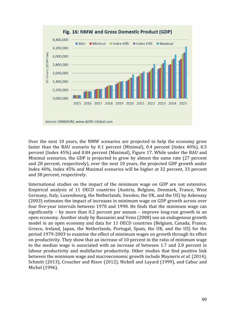
40
Over the next 10 years, the NMW scenarios are projected to help the economy grow faster than the BAU scenario by 0.1 percent (Minimal), 0.4 percent (Index 40%), 0.5 percent (Index 45%) and 0.84 percent (Maximal), Figure 17. While under the BAU and Minimal scenarios, the GDP is projected to grow by almost the same rate (27 percent and 28 percent, respectively), over the next 10 years, the projected GDP growth under Index 40%, Index 45% and Maximal scenarios will be higher at 32 percent, 33 percent and 38 percent, respectively.
International studies on the impact of the minimum wage on GDP are not extensive. Empirical analysis of 11 OECD countries (Austria, Belgium, Denmark, France, West Germany, Italy, Luxembourg, the Netherlands, Sweden, the UK, and the US) by Askenazy (2003) estimates the impact of increases in minimum wage on GDP growth across over four five-‐year intervals between 1970 and 1990. He finds that the minimum wage can significantly – by more than 0.2 percent per annum – improve long-‐run growth in an open economy. Another study by Bassanini and Venn (2008) use an endogenous growth model in an open economy and data for 11 OECD countries (Belgium, Canada, France, Greece, Ireland, Japan, the Netherlands, Portugal, Spain, the UK, and the US) for the period 1979-‐2003 to examine the effect of minimum wages on growth through its effect on productivity. They show that an increase of 10 percent in the ratio of minimum wage to the median wage is associated with an increase of between 1.7 and 2.0 percent in labour productivity and multifactor productivity. Other studies that find positive link between the minimum wage and macroeconomic growth include Mayneris et al. (2014), Schmitt (2013), Croucher and Rizov (2012), Nickell and Layard (1999), and Cahuc and Michel (1996).
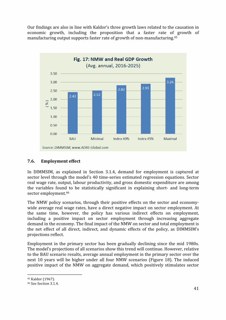
41
Our findings are also in line with Kaldor’s three growth laws related to the causation in economic growth, including the proposition that a faster rate of growth of manufacturing output supports faster rate of growth of non-‐manufacturing.45
7.6. Employment effect In DIMMSIM, as explained in Section 3.1.4, demand for employment is captured at sector level through the model’s 40 time-‐series estimated regression equations. Sector real wage rate, output, labour productivity, and gross domestic expenditure are among the variables found to be statistically significant in explaining short-‐ and long-‐term sector employment.46
The NMW policy scenarios, through their positive effects on the sector and economy-‐wide average real wage rates, have a direct negative impact on sector employment. At the same time, however, the policy has various indirect effects on employment, including a positive impact on sector employment through increasing aggregate demand in the economy. The final impact of the NMW on sector and total employment is the net effect of all direct, indirect, and dynamic effects of the policy, as DIMMSIM’s projections reflect.
Employment in the primary sector has been gradually declining since the mid 1980s. The model’s projections of all scenarios show this trend will continue. However, relative to the BAU scenario results, average annual employment in the primary sector over the next 10 years will be higher under all four NMW scenarios (Figure 18). The induced positive impact of the NMW on aggregate demand, which positively stimulates sector
45 Kaldor (1967). 46 See Section 3.1.4.

42
production and employment, is found to exceed the negative direct impact of the rise in sector average real wage rates on employment. Overall, the net effect of the two opposite forces on annual employment in the primary sector leads to improving the demand for employment, relative to the BAU scenario. Therefore, even though the downward trend in primary sector employment is expected to continue, the NMW policy will slow the decline. As a result, under all four NMW scenarios primary sector employment will be, on average, between 0.5 percent and 4.0 percent higher annually, relative to the BAU scenario results, as shown in Figure 18.
Relative to primary and service sectors, the NMW policy has the least effect on average wage rates in the manufacturing sectors (Section 7.2). Hence, the negative direct effect of the policy on manufacturing sector employment is limited, which allows for the policy’s positive effect on employment through the increase in aggregate demand to be unmitigated by a significant negative effect. Therefore, the impact of the NMW on manufacturing sector employment is projected to be positive and increasing over time. Relative to the BAU results, with a NMW policy, annual employment in the manufacturing sector is expected to gain momentum after 2017, and the gaps between the BAU likely future trend and the NMW results growing wider over time (Figure 19). However, even though the positive gap between the Minimal scenario results and BAU results is expected to stabilise after 2021, the corresponding gaps for the remaining NMW scenarios will continue to grow (Figure 19). Overall, the NMW scenario results show that, relative to the BAU scenario, annual manufacturing employment will be, on average, higher by 3.4 percent (Minimal), 7.2 percent (Index 40%), 7.4 percent (Index 45%) and 8.3 percent (Maximal). By 2025, these differences translate into 91 000 (Minimal), 234 000 (Index 40%), 260 000 (Index 45%) and 318 000 (Maximal) more employment in the manufacturing industries, relative to the BAU scenario.

43
In the service sector, relative to the BAU, the NMW policy scenarios are projected to lead to small positive increases in demand for employment for all service subsectors except two; in the case of Building Construction and Engineering and Wholesale, Retail Trade, Catering and Accommodation Services,’ the impact on their employment are projected to be negative. Overall, relative to the BAU results, average annual employment in the service sector is projected to be lower by 0.4 percent and 1.16 percent (Figures 18 and 19).
For the economy, as Figure 18 shows, the average annual employment effect of the NMW, relative to the BAU scenario, is projected to be zero (Minimal) to -‐0.3 percent (Index 40% and Index 45%). This translates into lower annual employment of 1 600 (Minimal) to 43 000 (Index 40% and Index 45%). In the case of the Maximal scenario, the scenario’s net effect on total employment is projected to be small and positive of about 30 000 or a 0.18 percent increase in total employment relative to the BAU scenario.
The unemployment outcomes of the NMW policy scenarios are presented in Figure 21 in terms of the average annual unemployment rate under the five scenarios. Overall, relative to the BAU scenario, the average annual unemployment rate under the four
Fig. 19: NMW and Employment
95
100
105
110
115
120
2015 16 17 18 19 20 21 22 23 24 2025
( BAU
= 100 )
NMW and TOTAL Employment(Relative to the BAU)
Minimal Index 40%Index 45% Maximal
95
100
105
110
115
120
2015 16 17 18 19 20 21 22 23 24 2025
( BAU
= 100 )
NMW and Primary Sector Employment(Relative to the BAU)
95
100
105
110
115
120
2015 16 17 18 19 20 21 22 23 24 2025
( BAU
= 100 )
Source: DIMMSIM, www.ADRS-‐Global.com
NMW and Manufacturing Employment(Relative to the BAU)
95
100
105
110
115
120
2015 16 17 18 19 20 21 22 23 24 2025
( BAU
= 100 )
NMW and Services Employment(Relative to the BAU)

44
NMW scenarios is projected to be between 0 percent (Minimal) to 0.2 percent (Index 40%) higher. Under the Maximal scenarios, the unemployment rate is projected to be 0.1 percent lower than the BAU scenario.
Our findings on the potential impact of the NMW on employment in South Africa are in line with the international consensus on the impact of minimum wages on employment. Although the debate on whether minimum wages negatively affect employment has been lengthy, the outcomes have been strikingly similar. Freeman (1995) summarised the earlier debate by stating, “The debate is over whether modest minimum wage increases have “no” employment, modest positive effects, or small negative effects. It is
Share (2014) Minimal Index 40% Index 45% Maximal Key Range (%)Agriculture, Forestry and Fishing 5.4% >5
Coal Mining 0.6% 3-‐4Gold, uranium and ore mining 0.8% 2-‐3
Other mining 1.9% 1-‐2Food 1.2% 0-‐1
Beverage 0.4% -‐1 -‐ 0Tobacco 0.0% (-‐2) -‐ (-‐1)Textiles 0.3% (-‐3) -‐ (-‐2)
Wearing Apparel 0.5% (-‐4) -‐ (-‐3)Leather and Leather products 0.0%
Footwear 0.1%
Wood and wood products 0.4%
Paper and paper products 0.3%
Printing, publishing and recorded media 0.4%
Coke & refined petroleum products 0.2%
Basic chemicals 0.2%
Other chemicals & man made fibres 0.4%
Rubber products 0.1%
Plastic products 0.3%
Glass and glass products 0.1%
Non-metalic minerals 0.4%
Basic iron & steel 0.2%
Basic non-ferrous metals 0.1%
Metal products excl.machinery 1.0%
Machinery and equipment 0.8%
Electrical equipment 0.3%
Tv, radio & communication equipment 0.0%
Professional & scientific equipment 0.1%
Motor vehicles, parts & accessories 0.6%
Other transport equipment 0.1%
Furniture 0.2%
Other industries 0.4%
Electricity, Gas and water 0.4%
Building construction and engineering 7.8%
Wholesale, retail trade, catering and accomodation services 24.1%
Transport, storage, and communication 5.4%
Financial services, business intermediation, insurance & real estate 15.1%
Community, social & personal services 29.6% 0.00% 0.00% 0.00%Other services 2.7%
Households 13.2% 0.00000% 0.00000% 0.0000% 0.00000%General government 13.7% 0.00000% 0.00000% 0.0000% 0.00000%
Total mining 8.7%
Total manufacturing 8.9%
Total services 82.4%
Total economy 100.0%
Fig. 20: EMPLOYMENT: NMW Scenarios vs. Base Scenario(NMW CAGR minus Base CAGR, 2015-‐2025)
Source: ADRS, Dynamically Integrated Macro-‐Micro Simulation Model (DIMMSIM), www.ADRS-‐Global.com
* Compound Annual Growth Rate (CAGR)
45
not about whether or not there are large negative effects.”47 Kuddo et al. (2015) synthesises findings from the more recent debate as follows:
“Although the range of estimates from the literature varies considerably, the emerging trend is that the effects of minimum wages on employment are usually small or insignificant (and in some cases positive).48 For example, based on a meta-‐study of 64 minimum wage studies published between 1972 and 2007 and measuring the impact of minimum wages on teenage employment in the United States, the most precise estimates were heavily clustered at or near zero employment effects.49 A meta-‐analysis of 16 U.K. studies found no significant adverse employment effect.50 In its re-‐examination of the job strategy, the OECD came to a similar conclusion, basing its policy advice on the considerable number of studies that have found that the adverse impact of minimum wages on employment is modest or non existent.51 Recent studies using natural experiments or detailed payroll data also point toward no significant effects on employment and some positive benefits such as reduced turnover and increased productivity.52”
Additionally, Belman and Wolfson (2014) use meta-‐analysis to provide a comprehensive evaluation of more than 200 published papers since 1991 on the effects of minimum wage increases. Their findings indicate that minimum wage increases result in “small and vanishingly small” declines in employment.53
47 Freeman (1995), p. 833; emphasis in original. 48 See Betcherman (2014); Belman and Wolfson (2014). 49 Doucouliagos and Stanley (2009). 50 Leonard et al. (2013). 51 OECD (2006). 52 Card and Krueger (1995, 2000); Dubeet al. (2010); Hirsch et al. (2011). 53 Dube et al.(2010) examine the impact of minimum wage increases on the most intensive users of minimum wage workers in the US, namely, accommodation and food services (hotels and other lodging places, restaurants, bars, catering services, mobile food stands, and cafeterias) and retail. They find a positive and significant treatment of minimum wages on earnings for the accommodations and food services sector and the estimated effect on employment is positive but not statistically significant. Overall, they find that “the estimated treatment effects [on earnings] are smaller in sectors with higher average wages, and no significant employment effects are discernible in any of these sectors. We conclude that our key findings hold when we examine the low-‐wage sectors more broadly.” (p. 961).
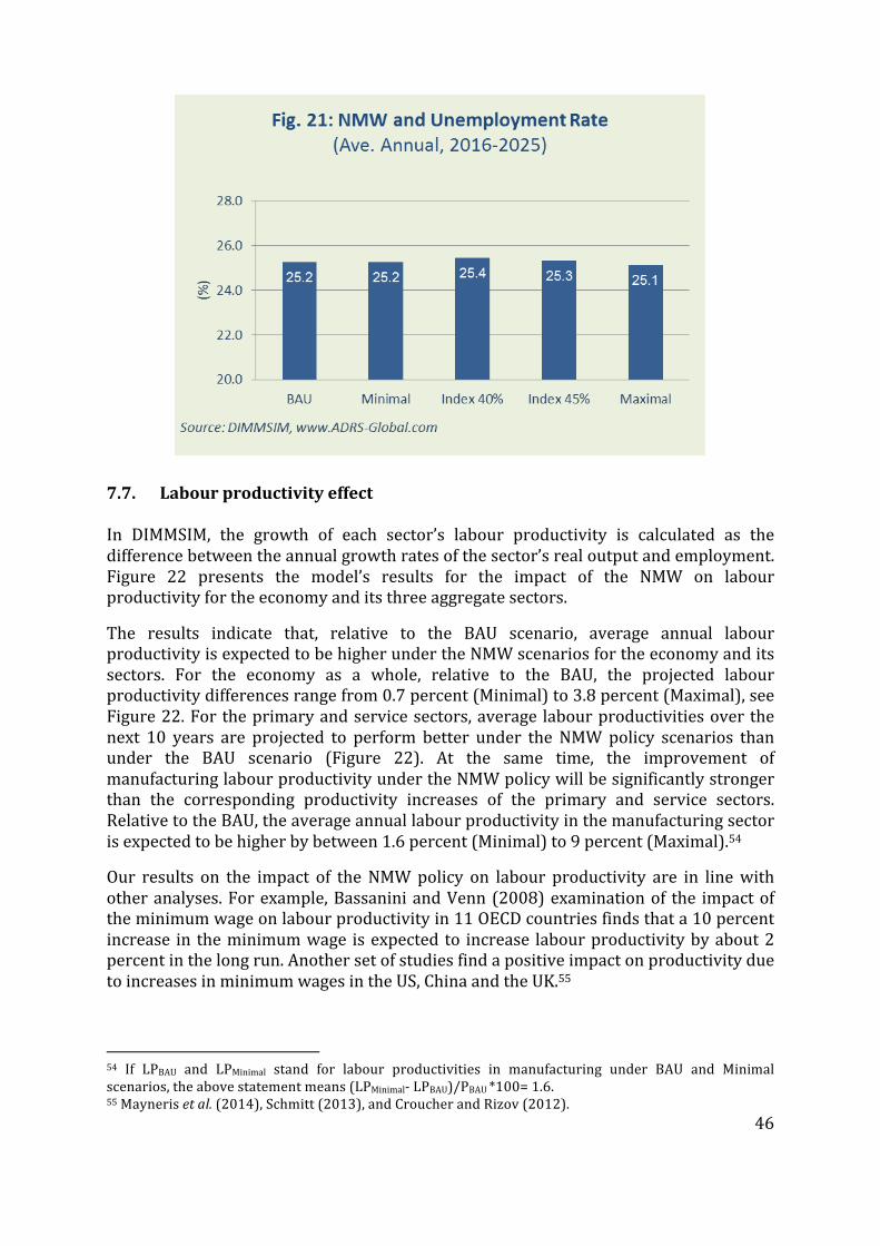
46
7.7. Labour productivity effect In DIMMSIM, the growth of each sector’s labour productivity is calculated as the difference between the annual growth rates of the sector’s real output and employment. Figure 22 presents the model’s results for the impact of the NMW on labour productivity for the economy and its three aggregate sectors.
The results indicate that, relative to the BAU scenario, average annual labour productivity is expected to be higher under the NMW scenarios for the economy and its sectors. For the economy as a whole, relative to the BAU, the projected labour productivity differences range from 0.7 percent (Minimal) to 3.8 percent (Maximal), see Figure 22. For the primary and service sectors, average labour productivities over the next 10 years are projected to perform better under the NMW policy scenarios than under the BAU scenario (Figure 22). At the same time, the improvement of manufacturing labour productivity under the NMW policy will be significantly stronger than the corresponding productivity increases of the primary and service sectors. Relative to the BAU, the average annual labour productivity in the manufacturing sector is expected to be higher by between 1.6 percent (Minimal) to 9 percent (Maximal).54
Our results on the impact of the NMW policy on labour productivity are in line with other analyses. For example, Bassanini and Venn (2008) examination of the impact of the minimum wage on labour productivity in 11 OECD countries finds that a 10 percent increase in the minimum wage is expected to increase labour productivity by about 2 percent in the long run. Another set of studies find a positive impact on productivity due to increases in minimum wages in the US, China and the UK.55 54 If LPBAU and LPMinimal stand for labour productivities in manufacturing under BAU and Minimal scenarios, the above statement means (LPMinimal-‐ LPBAU)/PBAU *100= 1.6. 55 Mayneris et al. (2014), Schmitt (2013), and Croucher and Rizov (2012).

47
7.8. Inflation effect In DIMMSIM, prices are represented by more than 120 time-‐series estimated equations that capture diverse demand and supply factors that determine various prices in the system. Therefore, the model’s 45 production, 27 consumption, and 45 investment price equations represent the influences of real, nominal, production, demand, and distribution factors on prices. A NMW policy is thus expected to affect various price categories not only through its direct effects on the cost of labour but also its indirect effects on income, expenditure, and production variables. Given space limitations, we present the model results solely for the economy-‐wide producer price index.
The results capture differences among scenarios in terms of the economy-‐wide producer price inflation, as shown in Figure 23. The average inflation rates for the BAU and the Minimal NMW scenarios are projected to be almost indistinguishable, which imply that, in the final analysis, the Minimal scenario’s NMW trajectory will have subdued effects on the average inflation rate over the next 10 years. In this case, a combination of relatively small increases in the average wage rate and labour productivity effectively annul their contradictory effects on price inflation. For the other NMW scenarios, their lower average inflation rates over the next 10 years, relative to the BAU scenario, reflect the extent that the negative effects of labour productivity increases on sector prices prevail over the positive effects of the scenarios’ average wage rate increases.

48
7.9. Inequality and poverty effects The main rationale for a NMW policy for South Africa is to reduce poverty and income inequality and to deter their future growth. In previous sections, the likely impact of four NMW policy scenarios on the wage rate, prices, employment, and household income and consumption were presented using the results from the macroeconomic module of DIMMSIM. However, since poverty and inequality analyses are conducted at individual and household levels in order to take account of important heterogeneities within the population, an assessment of the effectiveness of a NMW policy to achieve its main objective requires micro-‐level analysis of its impact. As discussed in section 3.2, DIMSSIM’s microsimulation component enables it to quantify the impact of policy scenarios on indicators of economic wellbeing of individuals, families and households, including poverty and inequality indicators. This section presents the outcome of the above process in terms of the impact of NMW policy scenarios on poverty and inequality.
Figure 24 shows that relative to the BAU results, in which there is no NMW, income inequality, measured by the Gini index, is projected to be lower under the four NMW scenarios. This reflects the effectiveness of economic growth paths that include the NMW policy to benefit the poor more than the non-‐poor. At the national level, the inequality indices for the four NMW scenarios in 2025 are projected to be lower than the BAU results by -‐0.4 percent (Minimal), -‐0.7 percent (Index 40%), -‐1.2 percent (Index 45%), and -‐1.7 (Maximal).
Figure 25 shows that the NMW policy is expected to produce lower rates of inequality among both urban and non-‐urban population. At the same time, the projections show that relative to the BAU results, for each NMW scenario, the decline in income inequality among the non-‐urban population will be more significant than the decline in the income inequality among the urban population. In other words, not only are both rates of

49
inequality projected to decline, but the difference in inequality between the urban and non-‐urban population is also projected to narrow with the NMW policy.
The model results on household poverty are summarised in Figures 26 to 29. We used the adult equivalent poverty line of R930 per month for 2016 that annually adjusts to the average inflation rate of 6 percent. At national level, relative to the BAU scenario, the model’s projections for the four NMW scenarios show improvements in the headcount poverty rate. The national poverty rate will be lower than the BAU scenario results for
-‐0.4
-‐0.7
-‐1.2
-‐1.7
-‐1.8 -‐1.6 -‐1.4 -‐1.2 -‐1
-‐0.8 -‐0.6 -‐0.4 -‐0.2
0 Minimal Index (40%) Index (45%) Maximal
( % )
Source: DIMMSIM, www.ADRS-‐Global.com
Fig. 24: NMW and Income Inequality (Difference with BAU, 2025)
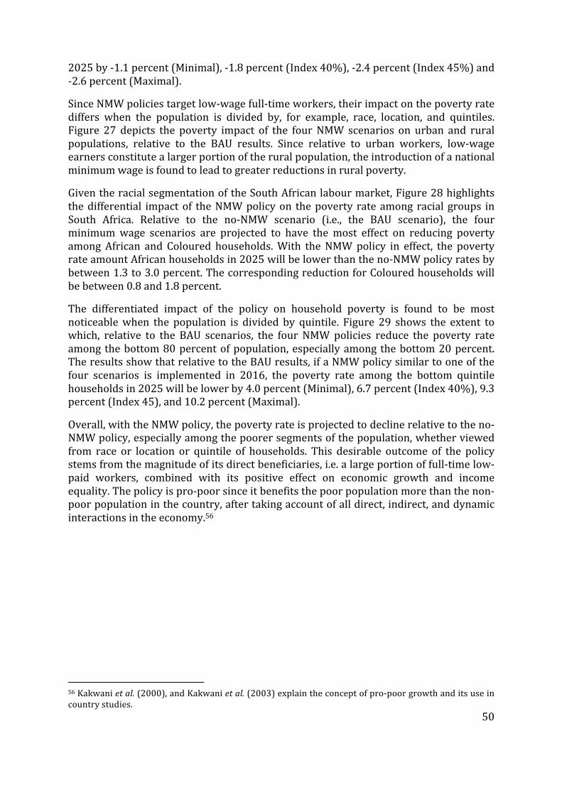
50
2025 by -‐1.1 percent (Minimal), -‐1.8 percent (Index 40%), -‐2.4 percent (Index 45%) and -‐2.6 percent (Maximal).
Since NMW policies target low-‐wage full-‐time workers, their impact on the poverty rate differs when the population is divided by, for example, race, location, and quintiles. Figure 27 depicts the poverty impact of the four NMW scenarios on urban and rural populations, relative to the BAU results. Since relative to urban workers, low-‐wage earners constitute a larger portion of the rural population, the introduction of a national minimum wage is found to lead to greater reductions in rural poverty.
Given the racial segmentation of the South African labour market, Figure 28 highlights the differential impact of the NMW policy on the poverty rate among racial groups in South Africa. Relative to the no-‐NMW scenario (i.e., the BAU scenario), the four minimum wage scenarios are projected to have the most effect on reducing poverty among African and Coloured households. With the NMW policy in effect, the poverty rate amount African households in 2025 will be lower than the no-‐NMW policy rates by between 1.3 to 3.0 percent. The corresponding reduction for Coloured households will be between 0.8 and 1.8 percent.
The differentiated impact of the policy on household poverty is found to be most noticeable when the population is divided by quintile. Figure 29 shows the extent to which, relative to the BAU scenarios, the four NMW policies reduce the poverty rate among the bottom 80 percent of population, especially among the bottom 20 percent. The results show that relative to the BAU results, if a NMW policy similar to one of the four scenarios is implemented in 2016, the poverty rate among the bottom quintile households in 2025 will be lower by 4.0 percent (Minimal), 6.7 percent (Index 40%), 9.3 percent (Index 45), and 10.2 percent (Maximal).
Overall, with the NMW policy, the poverty rate is projected to decline relative to the no-‐NMW policy, especially among the poorer segments of the population, whether viewed from race or location or quintile of households. This desirable outcome of the policy stems from the magnitude of its direct beneficiaries, i.e. a large portion of full-‐time low-‐paid workers, combined with its positive effect on economic growth and income equality. The policy is pro-‐poor since it benefits the poor population more than the non-‐poor population in the country, after taking account of all direct, indirect, and dynamic interactions in the economy.56
56 Kakwani et al. (2000), and Kakwani et al. (2003) explain the concept of pro-‐poor growth and its use in country studies.
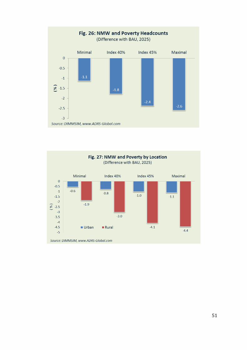
51

52
Similar to our results for South Africa, almost all national and comparative studies have found that minimum wages lead to a compression of the earnings distribution.57 They have also found that minimum wages help lower earning differentials across demographic groups, as have been reported for Brazil and Costa Rico.58 Since the minimum wage has significantly smaller impact on higher earnings, raising the
57 See overviews in Katz and Murphy (1992), DiNardo et al. (1996), Katz and Autor (1999), Card and DiNardo (2002), Autor et al.(2008), Goldin and Katz (2008), Lemieux (2008), and Acemoglu and Autor (2011). 58 Lemos (2007), Gindling and Terrell (1995), and Fajnzylber (2001).

53
minimum wage would effectively reduce earning inequality.59 Moreover, our results, that show a significant reduction in the poverty rate among the households in the bottom quintiles and a much smaller poverty reduction among households in higher quintiles, are in line with international studies that find between 40 and 60 percent of poverty benefits is concentrated in bottom households and that the benefits gradually die out. For example, Mishel et al. (1995) found that some 60 percent of the gains from minimum wage increases would accrue to the bottom 40 percent of families with at least one worker, and that the remaining gains persist across the entire distribution of families with one worker. Burkhauser et al. (1996) found that workers who live in poor families are 3.6 times more likely to be helped by a minimum wage hike than is the average worker.60
7.10. Comparison of NMW scenario performances The aim of the scenarios used in this study was to use a range of possibilities for the NMW that are distinct from each other in terms of the level of the NMW and/or mechanism that the scenario uses to annually update the national minimum wage rate(s) over time. The purpose therefore was neither to provide an exhaustive list of possibilities for the NMW in South Africa nor to arrive at a specific NMW for the country.
As we reviewed and analysed the model results for the BAU and four NMW scenarios, we noticed possible differences between the scenarios in terms of the volatility of indictors that were analysed in this report. We therefore estimated the degree of volatility of various indicators by calculating the standard deviations of various indicators used in the report for all the economic sectors over the forecast period of 2016-‐2025. The results show that relative to the BAU scenario, the Maximal scenario generates results that are relatively more volatile than all other scenarios. For half of indicators, the Maximal scenario exhibits highest volatility. High volatilities of economic indicators usually translate into increased uncertainty with regard to the future path of the economy, especially in the short run.
8. Conclusion The purpose of this research was to use economic modelling techniques to quantify the macro and micro-‐economic impact of four specific NMW policy scenarios for South Africa that were provided by the National Minimum Wage Research Initiative at CSID in the University of Witwatersrand who commissioned the study.
We have shown that a NMW in South Africa has the potential to yield positive overall macro-‐ and micro-‐economic outcomes. The introduction of the NMW would prompt direct, indirect and dynamic responses in the labour market, household income and 59 This was a result of a study on the British Wages Councils by Machin and Manning (1994). 60 Other important studies include Gindling’s (2014) study of the effectiveness of the minimum wage to reduce poverty and inequality in developing countries. Alaniz et al. (2011) and Gindling and Terrell (2010) found that a 1 percent increase in minimum wages lowered the incidence of poverty by 0.12 percentage points in Nicaragua and by 0.22 percentage points in Honduras. See also Card and Krueger (1995), Neumark and Wascher (1997), and Fields and Kanbur (2007).

54
expenditure, and production. Depending on its initial value(s) and its future evolution, it could meaningfully achieve its core goals of reducing poverty and income inequality. The net effect of the policy includes an upward shift of the aggregate demand curve and an outward shift of the aggregate supply curve, thus spurring modest stable macroeconomic growth. This overall macroeconomic outcome will be the result of the positive income distribution impact of the policy which is represented by an improvement in the income share and spending power of households in the bottom quintiles that have a relatively higher marginal propensity to consume (spend a relatively larger portion of each additional rand in income) but also spend a relatively larger portion of each additional rand on domestically produced goods and services. This redistributive impact of the policy will directly and indirectly, through the forward and backward linkages, stimulates demand for and output of economic sectors, specially the manufacturing sector. For more than 85 percent of economic sectors, this positive force outweighs the direct negative impact of marginally higher sectoral average wage rates on employment.
The study advances the current literature on the NMW in at least three ways:
First, it assesses the impact of the policy using a linked macro-‐micro model whose macroeconomic component’s analytical foundation, functional specification, and empirical estimation are based on neither neo-‐classical perfect competition and general equilibrium economics nor the calibration methods used in empirical CGE models. The model links a heterodox macroeconometric model of South Africa to a full household microsimulation model of taxes, transfers, poverty and inequality.
Second, the model used for the study takes account of heterogeneity in sectors of the economy, not just in terms of classification but more importantly in terms of significant variations in their economic performance. It captures the sectoral heterogeneity within the South African economy through time-‐series regression analysis of 7 sector level variables, thus making the model a truly bottom-‐up multi-‐sectoral macroeconomic model. Especially important for this study is the inclusion of sector-‐specific time-‐series estimated wage and employment equations, which include sector-‐specific estimated elasticities.
Third, relative to other South African and international studies, we have assessed the potential impact of a NMW policy on a much larger set of indicators within an integrated framework. This includes the examination of its impact on indicators related to the labour market (wages, employment, labour productivity), macroeconomy (income, consumption, inflation, GDP), and household poverty and inequality wages (headcount poverty, income inequality). The report therefore provides a more holistic view of the policy’s potential impact, which is especially useful for deciding whether a NMW is a good policy for South Africa.
Important findings include:
§ The report confirms other studies that the minimum wage is an effective policy to (modestly) foster aggregate demand and provides evidence of the positive spill-‐overs beyond the very bottom of the earnings distribution.

55
§ The results reported here cast, as in the majority of international studies, severe doubt on the claims that the introduction of a NMW in South Africa will seriously hinder employment.
§ The findings of this report also point to the importance of the role of demand as a determinant of growth in the long run.
§ The policy will make a demonstrable contribution in terms of reducing poverty and inequality, but it is not a silver bullet to fully overcome the three-‐pronged challenges of high poverty, inequality, and unemployment in the country.
§ Introduction of a NMW in South Africa has the potential to reduce poverty by enhancing economic growth and reducing income inequality.
§ The small negative effects on employment in few economic sectors neither threaten macroeconomic balance nor hinder economic growth. That seems an acceptable trade-‐off for a policy with significant positive contributions to household real disposable income, poverty alleviation, income equality, and economic growth.

56
References
Acemoglu, D., and D.H. Autor (2011). “Skills, Tasks and Technologies: Implications for Employment and Earnings.” in O. Ashenfelter and D. Card, eds. Handbook of Labor Economics. Vol 4B. Amsterdam: Elsevier-‐North Holland. Adelzadeh, A. (2001). “Social Policy Model for Fighting Poverty in South Africa.” Report prepared for the UNDP. -‐-‐-‐-‐-‐-‐-‐-‐-‐ (2016). “Macroeconometric Model of South Africa: Model Specification and Estimation.” Applied Development Research Solutions. Forthcoming. Agenor, P.R., A.Izquierdo, and H.Fofack (2003). The Integrated Macroeconomic Model for Poverty Analysis: A Quantitative Macroeconomic Framework for the Analysis of Poverty Reduction Strategies. World Bank Policy Research Working Paper No. 3092. Washington DC: The World Bank. Alaniz, E., T.H. Gindling, and K. Terrell (2011). “The Impact of Minimum Wages on Wages, Work and Poverty in Nicaragua.”Labour Economics, 18 (S1). Alonso, C. (2015). “Beyond Labour Market Outcomes: The Impact of the Minimum Wage on Nondurable Consumption.” Alton, T., A. Channing, R. Davies,F. Hartleya, K. Makrelova, J. Thurlowc, and D.Ubogu (2012).“The economic implications of introducing carbon taxes in South Africa.” UNU-‐WIDER Working Paper No. 2012/46, May 2012. National Treasury and United Nations University–World Institute for Development Economics Research. Available at: http://www.wider.unu.edu/publications/working-‐papers/2012/en_GB/wp2012-‐046/ Ashworth, S.G.E., N.M.H. MacNulty, and A. Adelzadeh (2002).“National and Sector Specific Social and Economic Implications of Selecting Capital or Labour Intensive Methods of Coal Production.” COALTECH 2020, Task 7.14.1. Askenazy, P. (2003). “Minimum wage, exports and growth.” European Economic Review, 47(1), pp. 147−164. Autor, D.H., L.F. Katz and M.S. Kearney (2008). “Trends in U.S. Wage Inequality: Re-‐Assessing the Revisionists.” Review of Economics and Statistics, 90(2), 300-‐ 323. Bassanini, A. and D. Venn (2008). “The impact of labour market policies on productivity in OECD countries.” International Productivity Monitor, 17(11). Belman, D. and P.J. Wolfson (2014). “What Does the Minimum Wage Do?” Kalamazoo, Michigan, U.S.A.: W.E. Upjohn Institute Employment Research. Betcherman, G. (2014). “Labor Market Regulations: What Do We Know about Their Impacts in Developing Countries.” The World Bank Research Observer.

57
Bhorat, H., B. Jourdan, R. Kanbur, C. Rooney, B. Stanwix, and I. Woolard (2015). “Investigating the Feasibility of a National Minimum Wage for South Africa.” DPRU. December. Böhringer, C. and T. Rutherford (2006). “Combining Top-‐Down and Bottom-‐up in Energy Policy Analysis: A Decomposition Approach.” ZEW Discussion Paper, No. 06-‐007. Bourguignon, F. (2004). “The Poverty-‐Growth-‐Inequality Triangle”, Paper Presented at the Indian Council for Research on International Economic Relations, New Delhi, February. Bourguignon, F., M. Bussolo, L.A. Pereira da Silva (eds.) (2008). The Impact of Macroeconomic Policies on Poverty and Income Distribution: Macro-‐micro Evaluation Techniques and Tools. Washington: Palgrave MacMilland and The World Bank. Bourguignon, F., J. de Melo, and A. Suwa, (1991). “Modelling the effects of adjustment programs on income distribution.” World Development, 19(11), pp. 1527-‐1544. Bourguignon, F., A.S. Robilliard, S. Robinson (2003).“Representative Versus Real Households in the Macro-‐economic Modeling of Inequality.” Working Paper. DIAL, CIPRE. Burkhauser, R.V., K.A. Couch and D.C. Wittenburg (1996). “Who Gets What from Minimum WageHikes: A Re-‐Estimation of Card and Krueger’s Distributional Analysis in Myth and Measurement: The New Economics of the Minimum Wage.’’ Industrial and Labor Relation Review, April, pp. 547-‐553. Cahuc, P. and P. Michel (1996.) “Minimum wage unemployment and growth.” European Economic Review, 40(7): 1463-‐1482. Card, D. and J. DiNardo (2002). “Skill Biased Technological Change and Rising Wage Inequality: Some Problems and Puzzles.” Journal of Labor Economics, 20(4), 733-‐783. Card, D. and A. Krueger (1994). “Minimum Wages and Employment: A Case Study of the Fast Food Industry in New Jersey and Pennsylvania.” American Economic Review, 84(4), September. -‐-‐-‐-‐-‐-‐-‐-‐-‐ (1995). Myth and Measurement: The New Economics of the Minimum Wage. Princeton: Princeton University Press. -‐-‐-‐-‐-‐-‐-‐-‐-‐ (2000). “Minimum Wages and Employment: A Case Study of the Fast-‐Food Industry in New Jersey and Pennsylvania: Reply.” American Economic Review, 90 (5). Castel-‐Branco, R. (2016). “Policy Considerations for the Design and Implementation of a National Minimum Wage for South Africa.” University of the Witwatersrand, Summary Report No. 2.

58
Cockburn, J. (2001). Trade Liberalization and Poverty in Nepal: A Computable General Equilibrium Micro-‐Simulation Analysis. Working Paper 01-‐18.CREFA, University of Laval. Cogneau, D. and A.S. Robillard (2000). “Income Distribution, Poverty and Growth in Madagascar: Micro simulations in a General Equilibrium Framework.” IFPRI TMD Discussion Paper No.61. Croucher, R. and M. Rizov (2012). “The Impact of the National Minimum Wage on Labour Productivity in Britain.” E-‐Journal of International and Comparative Labour Studies, Vol. 1, No. 3–4. In: http://adapt.it/EJCLS/index.php/ ejcls_adapt/article/view/43. Decaluwé, B., J.C. Dumont and L. Savard (1999). “How to Measure Poverty and Inequality in General Equilibrium Framework.” Laval University, CREFA Working Paper #9920. deJanvry, A., E. Sadoulet and A. Fargeix (1991). “Adjustment and Equity in Ecuador.” OECD Development Center, Paris. Dervis, K., J. de Melo and S. Robinson (1982). General Equilibrium Models for Development Policy. Cambridge: Cambridge University Press. DiNardo, J., N.M. Fortin and T. Lemieux (1996). “Labor Market Institutions and the Distribution of Wages, 1973-‐1992: A semiparametric approach.” Econometrica, 64(5), September, 1001-‐1044. Doucouliagos, H. and T.D. Stanley (2009). “Publication Selection Bias in Minimum-‐Wage Research? A Meta Regression Analysis.” British Journal of Industrial Relations. Dube, A., T. W. Lester, and M. Reich (2010). “Minimum Wage Effects Across State Borders: Estimates Using Contiguous Counties.” IRLE Working Paper, No. 157-‐07. http://irle.berkeley.edu/workingpapers/157-‐07.pdf Engle, R. and C. Granger (1987). "Co-‐integration and error correction: Representation, estimation and testing". Econometrica, 55 (2): 251–276. Estrades, C. (2013). “Guide to Microsimulations Linked to CGE Models: How to Introduce Analysis of Poverty and Income Distribution in CGE-‐based Studies.” AGRPDEP Technical Note TN 09, May. Fajnzylber, P. (2001). “Minimum Wage Effects throughout the Wage Distribution: Evidence from Brazil’s Formal and Informal Sectors.” Working Paper Series 151, Centro de Desenvolvimento e Planejamento Regional, Belo Horizonte, Brazil. Fields, G.S. and R. Kanbur (2007). “Minimum Wages and Poverty with Income-‐Sharing.” Journal of Economic Inequality, 5: 135-‐147
59
Finn, A. (2015). “A national minimum wage in the context of the South Africa labour market.” University of the Witwatersrand, Working Paper Series No. 1. Friedman, M. (1957). “The Permanent Income Hypothesis." InM. Friedman, A Theory of the Consumption Function. Princeton University Press. Freeman, R. (1995). “What will a 10%...50%...100% Increase in the Minimum Wage Do?” Industrial Labor Relations Review, 48(4): 830-‐834. Gindling, T.H. (2014). “Does Increasing the Minimum Wage Reduce Poverty in Developing Countries?” IZA World of Labor. Gindling, T.H. and K. Terrell (1995). “The Nature of Minimum Wages and Their Effectiveness as a Wage Floor in Costa Rica, 1976–91.” World Development, 23(8): 1439–1458. Gindling, T.H. and K. Terrell (2010). “The Impact of Minimum Wages on Wages, Work and Poverty in Nicaragua.” UMBC Economics Department Working Papers, 10-‐126, UMBC Department of Economics. Goldin, C. and L. Katz (2008). The Race between Education and Technology. Cambridge: Harvard University Press. Gunning, W.J. (1983). “Income Distribution and Growth: A Simulation Model for Kenya.” in D.G. Greene (principal author), Kenya: Growth and Structural Change. 2 vols. Washington, DC: World Bank, pp. 487-‐621 Hansen, B. (1992). “Efficient Estimation and Testing of Cointegrating Vectors in the Presence of Deterministic Trends.” Journal of Econometrics, 53, pp. 87-‐121. Harris B. and M. Kearney (2014). “The ‘Ripple Effect’ of a Minimum Wage Increase on American Workers.” Brookings, Up Front. http://www.brookings.edu/blogs/up-‐front/posts/2014/01/10-‐ripple-‐effect-‐of-‐increasing-‐the-‐minimum-‐wage-‐kearney-‐harris. Hirsch, B., B. Kaufman, and T. Zelenska (2011). “Minimum Wage Channels of Adjustment.” IZA Discussion Papers, 6132, Institute for the Study of Labor (IZA). ILO (2014). “Minimum Wage Systems.” International Labour Organisation Office, Geneva. http://www.ilo.org/wcmsp5/groups/public/-‐-‐-‐ed_norm/-‐-‐-‐relconf/documents/meetingdocument/wcms_235287.pdf Kakwani, N., S. Khandker and H. Son (2003). “Pro Poor Growth Strategies in Africa: Poverty Equivalent Growth Rates with applications to Korea and Thailand.” Economic Commission for Africa, Economic Policy Research Center, Expert Group Meeting, June. Kakwani, N. and E. Pernia (2000). ”What is Pro Poor Growth?” Asian Development Review, 18, 1–16.

60
Kaldor, N. (1967). Strategic Factors in Economic Development. New York: Ithaca. Kantor, B. (2015). “Unleashing the Household Sector.” Business Day Live (BDlive), 30 July.
Katz, L. and D. Autor (1999). “Changes in the Wage Structure and Earnings Inequality.” O. Ashenfelter and D. Card, eds. The Handbook of Labor Economics. Volume III, Amsterdam: Elsevier. Katz, L.F. and K.M. Murphy (1992). “Changes in Relative Wages, 1963-‐1987: Supply and Demand Factors.” Quarterly Journal of Economics, 107(1), 35-‐78 Konopelko, E. (2015). “Setting and Adjusting a National Minimum Wage.” University of the Witwatersrand, Policy Brief, No. 6. Koop, G., M.H. Pesaran and S.M. Potter (1996). “Impulse response analysis in nonlinear multivariate models.” Journal of Econometrics, 74, 119-‐47 Kuddo, A., D. Robalino, and M. Weber (2015). “Balancing Regulations to Promote Jobs: from employment contracts to unemployment benefits.” World Bank Group, 101596. Lau, L. (1984). Comments on Mansur and Whalley (1984), in H. Scarf and J. B. Shoven (eds), Applied General Equilibrium Analysis, Cambridge University Press, New York, pp. 127– 137. Lemieux, T. (2008). “The Changing Nature of Wage Inequality.” Journal of Population Economics, 21(1), January, 21-‐48. Lemos, S. (2007). “The Effects of the Minimum Wage in the Private and Public Sectors in Brazil.” Journal of Development Studies. Leonard, M., T.D. Stanley, and H. Doucouliagos (2013). “Does the UK Minimum Wage Reduce Employment? A Meta Regression Analysis.” British Journal of Industrial Relations.http://www.hendrix.edu/uploadedFiles/Departments_and_Programs/Business_and_Economics/AMAES/ UkMinWage%20final%20edits.pdf. Machin, S. and A. Manning (1994), “The Effects of Minimum Wages on Wage Dispersion and Employment: Evidence from the U.K. Wage Councils.” Industrial and Labour Relations Review, January, pp. 319-‐329. MacLeod, C. (2015). “Measuring the Impact of a National Minimum Wage.” Power Point presentation to NEDLAC. Mansur, A. and J. Whalley (1984). “Numerical Specification of Applied General Equilibrium Models: Estimation, Calibration and Data.” in H. Scarf and J. B. Shoven (eds). Applied General Equilibrium Analysis. Cambridge University Press, New York, pp. 69–127.

61
Mayneris, F., S. Poncet and T. Zhang (2014). “The cleansing effect of minimum wage: Minimum wage rules, firm dynamics and aggregate productivity in China.” CEPII Working ,No. Paper 2014-‐16. Mishel, L., J. Bernstein, E. Rassell (1995). “Who Wins with a Higher Minimum Wage.” Economic Policy Institute Briefing Paper, Washington D.C., February. Morrisson, C. (1991). “Adjustment, Incomes and Poverty in Morocco.” World Development, Vol. 19. No 11. pp. 1633-‐1651. Neumark, D. and W. Wascher (1997). “Do Minimum Wages Fight Poverty?” NBER Working Paper Series, No. 6127.August. Nickell, S. and R. Layard(1999). “Labor market institutions and economic performance,” Handbook of Labor Economics, in: O. Ashenfelter and D. Card (ed.), Handbook of Labor Economics. Vol. 3, pp. 3029-‐3084. OECD (Organisation for Economic Co-‐operation and Development) (2006). “OECD Employment Outlook 2006.” Paris. OECD (1998). “OECD Employment Outlook 1998: June.” OECD Publishing, Paris. DOI: http://dx.doi.org/10.1787/empl_outlook-‐1998-‐en Orcutt, G. (1957). “A New Type of Socio-‐economic System.” Review of Economics and Statistics, 58, pp. 773-‐797. Orcutt, G. (1967). “Microeconomic Analysis for Prediction of National Accounts.” in H. Wold, G.H. Orcutt, E.A. Robinson, D. Suits and P. de Wolff (eds), Forecasting on a Scientific Basis -‐ Proceedings of an International Summer Institute, Gulbenkian Foundation, Lisbon. Orcutt, G., M. Greenberg, J., Korbel, and A. Rivlin (1961). Microanalysis of Socioeconomic Systems: A Simulation Study. New York: Harper and Row. Pauw K. (2007). “Economy-‐wide modelling: an input into the long term mitigation scenarios process. Long-‐term mitigation scenarios input,” Report 4. University of Cape Town, South Africa: Energy Research Centre, 2007. Pauw, K. and M. Leibbrandt (2012). “Minimum wages and household poverty: General equilibrium macro-‐micro simulations for South Africa.” World Development, Elsevier, 40(4): 771-‐783. Pesaran, B. and M.H. Pesaran (1997). Working with Microfit 4.0: Interactive Econometric Analysis. Oxford: Oxford University Press. Pesaran, M.H. (1997).“The Role of Economic Theory in Modelling the Long Run”, Economic Journal, 107.

62
Pesaran, M.H., and Y. Shin (1998). “Generalized impulse response analysis in linear multivariate models.” Economics Letters. Elsevier, vol. 58(1), pages 17-‐29, January.
Pesaran, M.H., Y. Shin, and R.J. Smith (1996). “Testing for the Existence of a Long-‐Run Relationship.” DAE Working Paper No. 9622. Department of Applied Economics, University of Cambridge. Pesaran M.H., Y. Shin, and R.J. Smith (1999). "Bounds Testing Approaches to the Analysis of Long Run Relationships." ESE Discussion Papers 46, Edinburgh School of Economics, University of Edinburgh. Pesaran, M. H., Y. Shin, and R.J. Smith (2001). “Bounds testing approaches to the analysis of level relationships.” Journal of Applied Econometrics, 16, 289-‐-‐326. Piggott, J. and J. Whalley (1985). U.K. Tax Policy and Applied General Equilibrium Analysis New Developments in Applied General Equilibrium Analysis. Cambridge: Cambridge University Press.
Potter, S. (1998). “Nonlinear Impulse Response Functions.” Domestic Research Function. Federal Reserve Bank of New York.
Sargent, T.J. (1987). "The Consumption Function." In T.J. Sargent, Macroeconomic Theory. New York: Academic Press.
Savard, L. (2003). “Poverty and Income Distribution in a CGE-‐Household Micro-‐ Simulation Model: Top-‐Down/Bottom Up Approach.” CIRP´EE Centre interuniversitaire sur le risque, les politiques economiques et l’emploi. Working Paper 03-‐43. Schmitt, J. (2013). “Why Does the Minimum Wage Have No Discernible Effect on Employment?” Center for Economic and Policy Research. http://www.cepr.net/documents/publications/min-‐wage-‐2013-‐02.pdf. Statistics South Africa (2008). “Labour Force Survey.” September 2007, Statistical Release P0210, March, Pretoria. Taylor, L. and R. von Arnim (2006). “Modelling the Impact of Trade Liberalisation: A Critique of Computable General Equilibrium Models.” Oxfam Research Report.file:///C:/Users/Asghar/Downloads/rr-‐modelling-‐impact-‐trade-‐liberalisation-‐010707-‐en.pdf Thorbecke, E. (1991). “Adjustment Growth and Income Distribution and Equity in Indonesia.” World Development, 19(11), pp. 1595-‐1614. ______. (2000). “The Use of Social Accounting Matrices in Modeling.” Paper Prepared for the 26th General Conference of The International Association for Research in Income and Wealth Cracow, Poland, 27 August to 2 September 2000.

63
Wells, H. and A.P. Thrilwall (2003). “Testing Kaldor’s Growth Laws Across the Countries of Africa.” African Development Review, Vol. 15, Issue 2-‐3, pp. 89-‐105, December