WORKING PAPER SERIESNumber 44

Southern Africa Labour and Development Research Unit

byTaryn Dinkelman and Vimal Ranchhod

Evidence on the impact of minimum wage laws in an informal sector:

Domestic workers in South Africa

About the Author(s) and Acknowledgments

Dinkelman is at Princeton University. Ranchhod is a senior lecturer at the University of Cape Town. Without implicating them in any way, this paper has beneted from discussions with John Bound, Char-lie Brown, John DiNardo, David Lam, James Levinsohn, Justin McCrary, Jerey Smith and Gary Solon. We are very grateful to Nicola Branson for sharing her data on LFS sample weights with us.We also thank Debbie Budlender for helpful discussions about the South African labor regulation.

Recommended citation

Dinkelman. T and Ranchhod. V (2010) Evidence on the impact of minimum wage laws in an informal sector: Domestic workers in South Africa. A Southern Africa Labour and Development Research Unit Working Paper Number 44. Cape Town: SALDRU, University of Cape Town

ISBN: 978-0-9814451-5-1

© Southern Africa Labour and Development Research Unit, UCT, 2010

Working Papers can be downloaded in Adobe Acrobat format from www.saldru.uct.ac.za. Printed copies of Working Papers are available for R15.00 each plus vat and postage charges.

Contact DetailsVimal RanchhodEmail Addy: vimal.ranchhod@gmail.com

Orders may be directed to: The Administrative Officer, SALDRU, University of Cape Town, Private Bag, Rondebosch, 7701, Tel: (021) 650 5696, Fax: (021) 650 5697, Email: brenda.adams@uct.ac.za

Evidence on the impact of minimum wage laws in aninformal sector: Domestic workers in South Africa∗

Taryn Dinkelman and Vimal Ranchhod

Version: July 2010

What happens when a previously uncovered labor market is regulated? We exploit theintroduction of a minimum wage in South Africa and variation in the intensity of this law toidentify increases in wages and formal contract coverage, and no significant effects on employmenton the intensive or extensive margins for domestic workers. These large, partial responses to thelaw are somewhat surprising, given the lack of monitoring and enforcement in this informal sector.We interpret these changes as evidence that external sanctions are not necessary for new laborlegislation to have a significant impact on informal sectors of developing countries, at least in theshort-run. [107 words] (Keywords: Minimum wage, informal sector, Africa)

∗tdinkelm@princeton.edu, vimal.ranchhod@gmail.com. Dinkelman is at Princeton University. Ranchhod is asenior lecturer at the University of Cape Town. Without implicating them in any way, this paper has benefited fromdiscussions with John Bound, Charlie Brown, John DiNardo, David Lam, James Levinsohn, Justin McCrary, JeffreySmith and Gary Solon. We are very grateful to Nicola Branson for sharing her data on LFS sample weights with us.We also thank Debbie Budlender for helpful discussions about the South African labor regulation.

1

1 Introduction

What happens to wages and employment in the informal sector after the introduction of a

minimum wage in that sector? The vast minimum wage literature in economics has remarkably

little to say on this question, since the informal sector has more often represented the uncovered

sector in this research and has been used to help distinguish between models of the labor market.

For example, if the wage and employment effects of a formal sector minimum are mirrored by

opposite-signed responses in the informal sector, this is consistent with a segmented two-sector

labor market model.1 However, if informal sector wages increase (and employment decreases)

when a formal sector minimum is adjusted upwards, this is consistent with spillovers in an

integrated labor market, or possibly with “lighthouse effects”.2 In this paper, we extend the

minimum wage literature and investigate whether a minimum wage floor can have any effect when

directly applied to the informal sector, where the institutional environment for monitoring and

enforcement of penalties is weak. We use the introduction of the first minimum wage in South

Africa’s domestic worker sector in November 2002 to analyze what can happen in the short-run.

Whether a minimum wage can have any impact in the informal sector is broadly relevant

for understanding more about the process of labor market formalization in developing countries.

As economies develop, labor relationships shift from rural to urban areas and take place in larger

and larger firms; employees or their employers start to pay taxes and workers gain legal

protections, often including a guaranteed minimum rate of pay. Such protections, when enforced,

may improve working conditions and reduce poverty among the least skilled workers (Lustig and

McLeod (1997) summarize results from several studies), or may hinder the operation of markets

and negatively affect productivity (as in Besley and Burgess, 2004) and employment.3 For many

1See Brown (1988) for a discussion of two sector models in minimum wage studies.2Spillover effects into the informal sector or other formal uncovered sectors have been documented by many

researchers, particularly in Latin American countries. See Lemos (2009) for Brazil, Gindling and Terrell (2004) forCosta Rica, Maloney and Menendez (2004) for a variety of Latin American countries, Bell (1997) for Mexico andColombia. See also Cortes (2004) for the USA. Brown (1988) notes that in the US, a large fraction of workers earnthe minimum wage, even though they are employed by establishments not subject to the minimum wage law.

3In that paper, Besley and Burgess (2004) show how active and costly pro-worker regulation in the formalmanufacturing sector in India led to increased informality, reduced investment and lower labor productivity.

2

developing countries contemplating such regulation, resources for monitoring and enforcement are

limited. Most economic models of employer behavior require some penalty and a non-zero

probability of being audited to predict any effects of minimum wage regulations (see Ashenfelter

and Smith (1979) for the canonical model of minimum wage compliance).4 A first-order question

for many developing countries then is: what effects can be expected from new labor legislation

that is not monitored or enforced?

In this paper, we shed light on the effects of new labor regulation in a context without

active enforcement or clear penalties. We present an empirical example in which domestic work

employers face an extremely high minimum wage (set at the 70th percentile of the pre-law wage

distribution) with no effective penalties and no monitoring, and show that employers still choose

to respond to the law. We document immediate, large and partial adjustment of wages upwards in

the wake of the law and find no significant effects on the intensive or extensive margins of work, at

least in the short-run, 16 months after the law is introduced.5 We also show dramatic increases in

the fraction of domestic workers who have a formal contract of employment, after the law. This

South African case indicates that labor legislation may not require a degree of market formality in

order to be effective; rather, the introduction of the law may serve as a focal point for shifting

markets in the direction of becoming more formal.6

The domestic work sector is important in its own right, and is under-studied given its

4Despite the greater availability of resources for enforcement in developed countries, non-compliance with mini-mum wage laws is widespread. Ashenfelter and Smith (1979) note that compliance with the US Federal minimumwage was only 65% in 1973; Cortes (2004) reports that in 1997, as many as 40% of US workers who qualified werepaid less than the minimum wage; and non-compliance rates in excess of 50% have been reported for Mexico, Mo-rocco (Squire and Suthiwart-Narueput 1997) and other developing countries. See Neumark and Wascher (2007) for acomprehensive review of the literature on minimum wages from developing countries. All of the theoretical literatureon compliance with a minimum wage hinges on employers choosing an optimal level of compliance in the face ofpenalties and enforcement. See Grenier (1982), Chang and Ehrlich (1985), Bloom and Grenier (1986), Chang (1992),Lott and Robert (1995) and Weil (2005).

5One benefit of focussing on short-run effects is that there is little time for workers to sort across areas and relocatee.g. from rural to urban areas in search of higher wage jobs. In our data, roughly the same fraction of domesticworkers report starting their current job in the past year, both before and after the law (12% in September 2001 and14% in September 2003). The remainder had longer tenure. Unfortunately, we are unable to analyze tenure lengthin this paper, as this information was not collected in every year of the survey.

6The first minimum wage law introduced in the US in 1912 (in Massachussetts, for women) had some similarfeatures to our setting. One penalty involved newspapers “naming and shaming” non-compliant firms by publishingtheir names (Thiess, 1991).

3

prevalence over space and time. Historically, this sector has been important in developed

countries. Rubinow (1906) uses census data to show that over 1.2 million women were employed

in domestic work in the US in 1900. World-wide, the market for domestic workers currently

employs many millions of women: foreign workers employed in private households currently make

up around 10% of the labor force in a number of Middle Eastern countries (Kremer and Watt,

2006); Cortes and Pan (2009) document that foreign domestic workers constitute 6% of the

workforce in Hong Kong; while ILO data for OECD countries record an average of 100,000 female

domestic workers per country. The UK and Germany are at the high end of this range with

400,000 and 460,000 female domestic workers respectively. In South Africa, close to one in five

women– about one million women– work as domestic workers.

In most of these labor markets, the domestic work sector clearly fits the ILO’s definition

of ‘informal’, as it consists of one-employee enterprizes (households) in which labor relations are

predominantly uncontracted and without formal minimum wage or other protections. The small

scale of employers makes this sector costly for unions to organize.7 Work often extends beyond

simple housekeeping services and can require a great deal of trust, particularly when child-care is

involved or when the employer is absent during working hours. Additionally, and particularly in

Asia, Latin America and the USA, domestic workers are often foreign migrant workers with

tenuous legal status. This increases their vulnerability in the labor market.8 For example, in the

USA, domestic workers are largely undocumented and are not yet guaranteed all of the

protections of the National Labor Standards Act (e.g. they are not currently entitled to overtime

pay).9 We believe our analysis of the South African case sheds light on the short-run effects of

7The ILO defines “informal employment” as “all remunerative work (i.e. both self-employment and wage em-ployment), that is not registered, regulated or protected by existing legal or regulatory frameworks, as well as non-remunerative work undertaken in an income-producing enterprize. Informal workers do not have secure employmentcontracts, worker’s benefits, social protection or workers’ representation” (http://www.ilo.org/public/libdoc/ILO-Thesaurus/english/tr1746.htm).

8This idea of heightened vulnerability is not new. In 1906, Rubinow (1906) writes about the “servant girl’sproblem” and describes American preferences for hiring foreign women for domestic work as being related to the“greater ease of managing them”, which translates into “longer hours, perhaps lowers wages, more work and, ingeneral, conditions of service more favorable to the employer”.

9Recently, the state of New York became the first state in the USA to sign into law a Domestic Work-ers Bill of Rights. Among other rights, the new law ensures that domestic workers have notice of termina-

4

introducing minimum wage legislation to these informal and uncovered work relationships that are

globally prevalent.

The empirical exercise in this paper is straightforward. We evaluate the effects of South

Africa’s 2002 minimum wage law for domestic workers by exploiting time-series variation in the

application of the law and pre-existing cross-sectional variation related to the intensity of the law

to identify wage and employment effects. We use six waves of a biannual labor force survey (LFS)

from 2001 to 2004 to capture worker-reported wages, hours of work and employment over time at

relatively high frequency. Large shifts in the wage and earnings distributions of domestic workers

are evident in non-parametric kernel densities. We complement this with an analysis that adopts

the methods in Lee (1999).10 We combine the before-after variation in the law with cross-sectional

variation in the intensity of the minimum wage law to implement a difference-in-differences

strategy to statistically examine the effects of the law. Using just the before-after variation, the

analysis shows that domestic worker wages increase by about 20% in the 16 months after the law.

Comparing the change in wages (and hours of work) of domestic workers in places where the

median wage was far below the wage floor in the pre-period, to places where the median wage was

closer to the minimum, we find that wages increased by a significant and additional 10-15%,

post-law. In contrast, we find no significant reduction in hours of work (although measurement

error in this variable makes it difficult to precisely estimate any hours effects), nor any significant

change in the probability of a low-skilled female worker being employed as a domestic worker in

the pre- versus post-period, in high wage gap compared to lower wage gap areas.11

In the typical difference-in-differences research design that exploits a change in policy at

tion, receive paid sick days and holidays, and other basic labor protections that are standard in the Fair La-bor Standards Act. See the editorial “The Rights of Domestic Workers”, The New York Times June 15, 2009.httP : //www.nytimes.com/2009/06/15/opinion/15mon3.html Also the article “Senate Passes Historic Bill To Pro-tect Domestic Workers” at http : //www.nysenate.gov/press− release/senate− passes−historic− bill− protect−domestic− workers posted on June 2, 2010.

10In that paper, Lee (1999) uses regional differences in the relative level of the US federal minimum wage to identifythe effects of the minimum wage law on wage inequality in the 1980s, separately from the effects of national trendsin wages.

11While there are changes in the observable characteristics of domestic workers after the law, adjusting for thiscompositional change does not account for the entire shift in the distribution of domestic worker wages in the wakeof the law. We show this in an appendix.

5

one point in time, a key identification assumption is that both the exposed and unexposed groups

are on the same trend in the absence of the policy change. In our scenario, all areas are exposed

to the law, but we make use of the fact that this law is more demanding of employers in areas

with lower pre-law wages. However, since the minimum wage is set so high in the pre-law wage

distribution, we expect to see (and do find) that domestic workers in all areas experience higher

wages in the immediate months after the law. Unlike other difference-in-differences approaches to

minimum wage policy changes, we are interested in the simple pre-post “difference” in wages as a

potential outcome of the new law. To provide evidence that the generalized wage increases we find

for all domestic workers is not solely the result of economy-wide shocks, we perform one placebo

experiment. We estimate the difference-in-differences specification for a set of similar workers who

are unlikely to compete over jobs with domestic workers, but whose job conditions likely reflect

general economic conditions: low-skilled male manufacturing workers in urban areas. We find that

in the period after the law, male manufacturing wages increase by about 10%, suggesting some

improvement in the economy after 2002. However, we can reject that these pre-post changes for

manufacturing workers are the same as for domestic workers: domestic workers as a group still

experience a significantly larger gain in wages (10%) in the period after the law. Furthermore, we

find no evidence that wages for male manufacturing workers rise more in areas where the

minimum wage law was more binding on domestic workers. This gives us more confidence that the

difference-in-differences results we estimate for domestic workers are not being driven by

differential wage trends between high and low wage gap areas.

One limitation of our analysis is that the data do not allow us to rule out that employers

achieved these wage increases by making offsetting reductions in non-wage in-kind benefits. These

benefits, mainly in the form of free food, were fairly substantial for some workers before the law,

as we describe. In order to show that the new law did have a substantive impact on the conditions

of work for domestic workers (outside of any wage increases), we also examine the probability that

a domestic worker has a formal job contract with their employer, after the law. We find that the

probability of an employee having a formal contract doubles in the 16 months after the law,

6

regardless of the intensity of the minimum wage floor in their area of work. This evidence on

contract coverage reflects the beginning of the formalization of this industry, which could have

far-reaching consequences for the nature of domestic work in the country.

Given the weak institutional environment for enforcement of the law, which we describe,

it is somewhat surprising that we see such large wage responses and no employment effects in this

informal sector. Isolating the exact reasons for the employer response is not easy; however, we

propose two pieces of evidence that suggest that employers were voluntarily and only partially

responding to the law. First, we develop a test for partial compliance, which shows that some

workers get increases bringing their wages closer to, but not nearly up to, compliant levels. This

partial compliance probably contributes to the lack of employment effects of the law.12 Second, we

show that the wage response of employers is not significantly different across places with different

audit probabilities, where we use the presence of a local Labour Centre (LC) as a proxy measure

of this probability. Partial compliance that does not appear responsive to the likelihood of audit is

consistent with the idea that employers may not have been primarily motivated by threat of

external sanctions.

Two related and unpublished papers have examined the effect of the minimum wage law

for domestic workers in South Africa: Hertz (2006) and Yamada (2007). Our study differs from

these studies in several dimensions. First, we focus on urban workers only, because we believe that

identification of the impact of the new minimum wage law for rural domestic workers is likely

confounded by the concomitant introduction of a minimum wage for agricultural workers, a

plausible alternative sector for low-skilled workers in rural areas.13 Second, we use an updated and

consistent set of survey weights for the LFS data (Branson, 2009) which were not available for

these studies.14 Third, we use a higher level of aggregation (the province) to define areas in which

12This finding relates to a theoretical point made in a recent paper by Basu, Chau and Kanbur (2007). Theauthors develop a model in which governments accept some non-compliance with minimum wage legislation toachieve distributional goals.

13Agricultural workers received protection under a minimum wage law, also for the first time, 6 months after thedomestic worker minimum wage floor was imposed.

14Details of this choice are discussed in the data section.

7

the new law was more or less binding, based on pre-law characteristics. This choice presents other

challenges for inference, which we describe in detail in our empirical approach section.15 Our

results for the wage effects of the minimum wage law turn out to be quite a bit smaller than the

estimates in Hertz (2006) and Yamada (2007) and, unlike these studies, we find very little evidence

for a negative employment effect of the law on either the intensive or extensive margins of work.

The paper begins with a description of the domestic worker industry in South Africa

before the law and describes the characteristics of the new law introduced in 2002. After

describing the data and presenting summary statistics of our sample, we turn to documenting the

wage, earnings, employment and hours of work effects of the law using a combination of kernel

densities for wages and earnings and difference-in-differences regressions. We discuss our test for

and present evidence of partial compliance with the law. We show that wage increases are not

larger in places with higher probability of audit, and that the law increased the probability of a

domestic worker having a formal employment contract, regardless of how large the initial wage

gap in the province of residence was. We conclude with a discussion and interpretation of results.

2 The domestic worker industry in South Africa

The domestic worker industry in South Africa employs 18% of all women, and 80% of all domestic

workers are female. Poorly educated African and coloured women make up the vast majority of

these domestic workers.16 In each year of our study, about 15% of urban African and coloured

female workers were in the domestic work sector. Unlike many Latin American and Middle

Eastern settings, and more like countries in the rest of Africa and parts of India, the majority of

15Hertz’s 2006 working paper uses some of the same LFS cross-sectional data to estimate the impact of the law onwages and employment using a difference-in-differences approach that relies on a much smaller unit of analysis (themagisterial district). He relates the intensity of the minimum wage law to the fraction of workers in a magisterialdistrict who initially earned below the minimum (following Card and Krueger, 1997). We choose not to use magisterialdistricts as the unit of analysis, since many districts contain only a few (under 10) individuals in each wave who areemployed as domestic workers.

16Following much of the economic literature on South Africa, we use apartheid-era racial classifications: Africanfor Black South African, and coloured for individuals of mixed race.

8

domestic workers in South Africa are not foreigners. Table 1 presents means and standard

deviations of female domestic worker demographics for each survey period before the law is

enacted (September 2001, March 2002), the “cusp” survey wave of September 2002, and the three

surveys after the law (March 2003, September 2003 and March 2004). All statistics are weighted,

and the data sources are described in more detail in the next section.

Immediately obvious from Table 1 is the remarkable stability of worker characteristics in

this industry. About 60% of domestic workers are urban workers, and within the urban group –

our sample of interest – the average age of workers is around 40. The majority are African and

have between 6.3 and 7.1 years of education (completed primary school). This is 0.8 to 2 years

below the average education of women working in the most closely related skill-groups: women in

elementary occupations (e.g. newspaper vendors, office cleaners, hawkers, building caretakers,

garbage collectors etc) and the female self-employed. 76% or more of domestic workers report

working full-time, defined as 28 hours or more per week, making the majority subject to the

full-time minimum wage.

Domestic workers are poorly remunerated. Mean wages are lower in this occupational

group than in any other: the ratio of the mean domestic worker wage to the mean wage for other

low-skilled African and coloured elementary workers (self-employed women) was 0.49 (0.64) in

September 2001. Prior to November 2002, there was no minimum wage in the domestic worker

sector and no formal mechanism existed for domestic workers to negotiate wages. Wages were

typically set unilaterally by the employer household or in consultation with other local employers

(see Cock (1989) for a qualitative description of this process). Some aspects of the 1997 South

African Basic Conditions of Employment Act governed overtime provisions, leave considerations,

minimum notice periods, fair dismissal procedures and severance pay for all workers (Department

of Labour, 1997). However, these were rarely adhered to in this informal market (Louw and Van

der Berg, 2004). Only 10% of domestic workers had a formal contract of employment in 2001,

compared to 55% of elementary occupation workers.

9

Remuneration for domestic work often combines cash and in-kind benefits. In another

survey (the 2000 South African Income and Expenditure survey, results not shown) which

captures information from employers about the value of food, clothing, accommodation and

unemployment benefits provided to the worker, about 25% of domestic worker employers report

providing the employee with some housing; 3% report unemployment insurance (UI) benefits, 34%

report some clothing provided to the employee, and the vast majority of employers, 80%, report

providing free food to employees. Averaging over all domestic worker households, we find that the

fraction of total remuneration accounted for by these benefits is low for UI (0.6%), clothing (6%)

and housing (5%), and highest for food (20%).17 Since a large fraction of total remuneration

comes from in-kind benefits before the law, it is plausible that employers may adjust benefits

downward to afford the wage increases. This will be an important caveat to the interpretation of

our wage results.

In setting the first national minimum wage for domestic workers, the Department of

Labour (DoL) took into account the recommendations of a government-appointed Employment

Conditions Commission. This group of government representatives and academics defined the

scope of the Domestic Worker Sector and concluded that any wage floor should “improve the

livelihoods of those worst off” and “retain jobs”. Their recommendation for the actual minimum

wage level was higher than that initially proposed by the government, and was the one eventually

adopted (Budlender et al, 2002).

Under the new law, which became effective on 1 November 2002, domestic workers and

gardeners working in private homes had the right to a minimum wage and to 8% annual wage

increases.18 The urban full-time hourly minimum wage was set at ZAR4.10 (USD 0.410) in

November 2002; the part-time wage was ZAR4.51 (USD 0.451) where part-time work is defined as

17We get these fractions by dividing the employer-reported value of food, accommodation, clothing and UI providedper month by the total monthly remuneration (cash plus benefits) reported by the employer. The more recent IESin 2005/2006 does not contain these data and so we cannot compare how these in-kind benefits may have changedover time.

18Garden workers, most of whom are men, are also covered as domestic workers under this law. However, theymake up a minority of domestic workers and so we omit them from our analysis.

10

fewer than 28 hours per week. In addition, the new law enabled employers to deduct up to 10% of

the total salary for rental value of any accommodation provided. A separate and related piece of

legislation, introduced shortly afterwards on April 1, 2003, additionally required employers to

register domestic workers with the DoL in order to pay unemployment insurance (UI).19

It is important to note that the changes introduced in this industry are an order of

magnitude larger than typical changes in the value of the minimum that economists typically

study: the wage floor was set at 1.5 times the median monthly earnings of domestic workers in

2002. Full compliance in this context would have entailed massive wage increases for a majority of

workers and potentially large employment effects for most employees either on the extensive or

intensive margin. Given existing high levels of unemployment in South Africa, this would be one

possible reason for why the government did not commit substantial resources towards enforcement

of the law.

In fact, in the first ten months after the law, both the audit probability and penalty for

first time violators were very small.20 As far as we have been able to establish, no inspections were

carried out until August 2003, ten months after the law. At this time, 1,600 households in five

provinces were earmarked for inspection and 25% of them were found to be in compliance with the

law.21 We have not been able to obtain further statistics on household inspections from the DoL.

There were also no documented rules about penalties or back-pay for non-compliers at the

time of implementation. Press releases from the DoL in February 2003 indicated that

“Non-compliance with the UI law will result in penalties of up to ZAR5,000 (USD500) per

19The average Rand/USD exchange rate from June 2002-January 2003 of ZAR10=USD1.20During this time, employers might have expected a vanishingly small audit probability for two reasons. First,

the chances of random inspection are small since inspections are labor intensive and each household yields only asingle worker inspection. If each domestic worker works in only one household, this yields over one million employersthat are subject to the minimum wage law. Second, logistical difficulties in gaining access to employer premises makeany inspection costly. A non-compliant employer can legally refuse to allow an inspector into their private residence,or simply not be present at the time of the inspection. A court order from a Labor Court is then required to enterthe residence. There are also physical barriers to entry: inspectors have reported difficulties with impenetrable gatesand “the presence of dogs” (Official release by the DoL, 27th August 2003. Available at www.labour.gov.za).

21See media release at www.labour.gov.za/media/statement.jsp?statementdisplayid = 9685

11

household or five years imprisonment”22. However, we have not been able to find formal

documentation of this or other penalties, nor has our search of newspaper archives revealed any

reports of fines or prison sentences being imposed on non-compliant employers.23 What we do

know is that non-compliers might have expected three progressively more threatening warnings

(telephonic, written, court order) before appearing at a court of law. At this time, they would

have had a right of appeal, which would be well exercised as it is unclear how evidence for

non-compliance would be substantiated in this predominantly cash payment industry.24

All evidence from the DoL website and various legal documents and reports related to the

law suggest that the general monitoring and enforcement regime in the domestic worker industry

was weak and presented employers with an almost zero expected cost of non-compliance. Despite

this lack of compliance incentive, the timing of the law coincides with substantial rightward shifts

in the wage and earnings distributions of domestic workers. We document this after describing our

data.

3 Data description and empirical methods

3.1 LFS Surveys

We use six cross sections of data from the nationally representative South African Labour Force

Surveys (LFS): September 2001, March 2002, September 2002, March 2003, September 2003 and

March 2004. These LFS surveys are biannual rotating panel surveys, conducted in

February/March and September each year and include detailed data on work and unemployment

experiences of 60,000 to 70,000 working-age individuals living in 30,000 households. The six waves

22http://www.info.gov.za/speeches/2003/03050809461001.htm23The Basic Conditions of Employment Act (1997) which covers all formal sector workers states that underpayment

violations are penalized in the following manner: first offence - 25% of the gap plus interest; second offence within 3years - 50% of the gap plus interest; third offence within 3 years or second offence within 2 years - 75% of the gapplus interest; fourth offence within 3 years - 100% of the gap plus interest; fifth offence within 3 years - 200% of thegap plus interest.

24Pay slips are now required as part of the minimum wage legislation.

12

we use span the period just before and just after the minimum wage law becomes effective in

November 2002. The survey instrument is similar to the US Current Population Survey, although

the rotation pattern differs. In each wave, 20% of households interviewed in the previous wave are

rotated out of the survey entirely.25 These LFS data are high frequency and can be used to

examine differences over a six month window. They help us to estimate the immediate impacts of

the law while controlling for observable characteristics of domestic workers (i.e. age, race and

years of education) and to see whether pre- versus post comparisons are sensitive to these controls.

We also model the probability of being employed as a domestic worker in each wave, using the set

of employed and unemployed women with similar age and education profiles to domestic workers.

We use these LFS data as repeated cross sections and exploit the cross-sectional variation in

intensity of the law at the province level (9 provinces in total) in combination with the time-series

variation in the law’s intensity to identify the effects of the law. 26

3.2 Sample weights

One further aspect of the data that is worth noting concerns the appropriateness of the sample

weights available in the LFS. Survey weights for LFS 2001 and 2002 are benchmarked to the 1996

Census; while survey weights for LFS 2003 are benchmarked to the later 2001 Census. With

different benchmark years, this series of weights is potentially inconsistent over time. Hertz (2006)

provides a detailed discussion of how these inconsistencies in the weights may affect any analysis

25Although there are three earlier waves of data going back to 2000, the baseline sample was drawn anew for theSeptember 2001 round which is why we begin our analysis with data from this round. And, although the LFS surveyhas continued biannually since March 2004, we cannot use additional waves of post-data in our analysis since thesurvey stopped reporting whether the individual resides in an urban or a rural area, thus making it impossible forus to condition our sample on urban domestic workers.

26There is a panel data component of the LFS survey, but we have some concerns about the representativenessand quality of the panel data set of workers. First, since the design of the panel includes a 20% out-rotation ofdwellings in each six month period, in order to appear in the panel a worker needs to be living continuously in thesame place for six waves and needs to escape the out-rotation group. We expect that workers who are more likelyto retain employment are also more likely to appear in the panel, making the estimation of the effects of the law onsuch a selected sample difficult. Second, we learned from Statistics South Africa (the organization that collects theLFS data) that some panel matches could not be made, because some fraction of questionnaires from the pre-periodwere lost in a flood. We have no way to know what impact this would have on the representativeness of the panel.

13

of the minimum wage law. He points out that the 2001 Census under-counted the fraction of

women of working age and that the extrapolations between 1996 and 2001 overestimated growth

in the adult population by underestimating the effect of the HIV epidemic on adult totals. He

notes that “no consistent official series of sampling weights is available. This poses a serious

problem, as both the changes in scale and the changes in the age, gender, province, and race

group distributions result in artifactual changes in the measured employment of domestic workers

that are too large to be ignored.” Indeed, the original sample weights that he refers to have been

shown to produce inconsistent aggregate statistics over time. More formally, Branson (2009)

explains that “The StatsSA weights presented in the data are problematic for analyses over time

... the auxiliary data used as a benchmark in the post-stratification adjustment are unreliable and

inconsistent over time and hence result in temporal inconsistencies even at the aggregate level.”

For these reasons, we do not use the weights provided with the LFS data. Rather, our

results use new (individual-level) survey weights that have been constructed by Nicola Branson

(2009) using entropy estimation.27 These weights produce “consistent demographic and

geographic trends”, as Branson (2009) shows.

3.3 Sample selection, key variables and empirical strategy

Our sample of workers includes all urban African and coloured woman aged 20 to 59, who report

domestic work, who do not also own their own business and who have no more than high school

education. For the employment analysis, we use an expanded sample of all African or coloured

woman aged 20 to 59 who live in urban areas, who have no more than a high school level of

education and who are employed or looking for work. For the placebo test, we make use of a

sample of male urban African and coloured workers, aged 20 to 59, who have no more than a high

27These methods are described in Branson (2009). Briefly, the idea is to create a new set of weights that are asclose to the original weights as possible (to preserve the main features of the sample design) but that are adjustedto account for errors arising from time inconsistent benchmarks, from inconsistencies between household and personweights, and for errors in the trimming of weights in earlier survey years. We are grateful to Branson for makingthese weights available to us.

14

school education and who report working in the manufacturing sector.

In the LFS, all workers are asked about earnings, pay frequency and usual weekly hours of

work. Most workers report earnings and a corresponding pay frequency. The vast majority– 89%

of domestic workers – report a monthly pay frequency. We convert all earnings to monthly

amounts using the pay frequency information. About 8-9% of domestic workers in any one wave

do not report earnings at all and we exclude these individuals from our analysis.28 To capture

hours of work, we use the response to the question “How many hours do you usually work in a

week?” We construct hourly wage measures by dividing monthly earnings by monthly hours. We

construct monthly hours as Usual hours worked per week∗Average weeks in a month. Just over

5% of workers report working more than 70 hours a week and we exclude these individuals from

our analysis.

We describe the impact of the minimum wage law in two ways. First, we estimate

non-parametric kernel densities of domestic worker wages and earnings and test for differences in

the domestic worker distributions over time using Kolmogorov-Smirnov tests of the equality of

distributions. Then, we statistically test for whether outcomes changed in the period after the law

compared to before the law, and for whether these changes are larger in areas where the minimum

wage initially had more “bite”. We specify the following difference-in-differences regression model:

yijt = α0 + α1POSTt + α2WGj + α3POSTt ∗WGj +Xijtγ + νijt (1)

where yijt is one of four main outcome variables for individual i living in province j in

period t: log hourly wages, weekly hours of work, the possession of a formal job contract for the

set of domestic workers, and whether the individual is employed as a domestic worker or not,

among the set of demographically similar women. Equation (1) is estimated with and without

controls for worker characteristics (Xijt), including age, years of education and an indicator

variable for whether the person is African. We group data from the September 2001, March 2002

28The fraction of domestic workers with no earnings information is not significantly different across waves.

15

and September 2002 surveys into a “Pre” period and the remaining three waves into the “POST”

period. Because the law was formally announced on August 30, 2002, but employers were only

expected to be compliant from 1 November 2002, there is some ambiguity about whether the

September 2002 wave belongs in the pre- or post-period. There was substantial publicity in the

months prior to the law becoming effective, making it plausible that some employers started to

react even before the November 1st deadline. For this reason, we also present results from

regressions that omit the September 2002 cusp wave, for which “POSTt” is not well-defined.

These are our preferred estimates.

To construct a measure of the intensity of the minimum wage law, we follow other

examples in the minimum wage literature (notably Lee, 1999) that use aggregate (rather than

individual) data on workers over time and construct a locally-specific wage gap using data on

wages from the “PRE” period. We define the province-level wage gap as:

WGj = log[min(w)] − log[median(wj)] (2)

where min(w) is the urban full-time minimum wage in November 2002 and median(wj) is

the median wage of all urban domestic workers in the province before the law. That is, the

intensity of the minimum wage law is measured according to domestic worker conditions in local

labor markets in September 2001 and March 2002.

The parameter α2 represents the average difference in outcomes for domestic workers in

low wage gap versus high wage gap areas across the entire period. α3 is the

difference-in-differences parameter and tells us how much more outcomes changed, in areas where

the minimum wage was most binding. In order for α3 to identify the effect of the minimum wage

law in high WGj areas, we must assume that in the absence of the law change, low wage gap

provinces would be on the same trend in outcomes as high wage gap provinces.

In addition to α3, α1 is also a parameter of interest as it tells us how wages (and other

16

outcomes) for domestic workers changed on average after the law. In most difference-in-differences

analyses this parameter is not directly of interest and the POSTt variable is included simply to

absorb common, contemporaneous shocks to outcomes or common trends. However, in the context

of this study, the minimum wage floor cuts so high in the distribution of domestic worker wages

that we expect at least a portion of α1 to reflect the impact of the law on average domestic worker

outcomes. This claim is, of course, difficult to make in the absence of evidence on economy-wide

trends in other wages. So, as a placebo test, we implement the same regression model as in (1) for

a set of workers for whom the minimum wage law is irrelevant and who do not directly compete

with domestic workers for jobs. These workers are male, low-skilled manufacturing workers in

urban areas. The minimum wage law for domestic workers does not apply to them and, moreover,

is set at a level far below their median wage. Changes in male manufacturing wages and hours of

work give us some indication of what is going on in the South African economy at the same time

as the new minimum wage law comes into place. We will be interested in testing whether α1 and

α3 are the same for the sample of manufacturing workers and domestic workers. If α1 is different,

this implies that the coefficient on POSTt in the domestic worker regression captures some of the

impact of the new law, over and above any economy-wide shocks to wages. If α3 is different, this

implies domestic worker wages (or other outcomes) are changing more in high wage gap relative to

low wage gap areas, and that these differential changes are not simply a reflection of broad trend

differences across high wage gap and low wage gap areas.

Note that our measure of the intensity of the law, WGt, is captured at the provincial level.

This means that in estimating (1), we exploit variation at the group (province) level to identify

the effects of the law. The fact that there are only nine groups (provinces) presents a challenge for

inference. Consider the following error components model for the error term νijt in (1):

νijt = vj + εijt (3)

Standard OLS without adjustment of the standard errors treats each individual as if they

17

contribute equally and independently to the variation in outcomes. Since σν = σv + σε and vj is

the same for each individual in the same province (the main policy change occurs at an aggregated

level), this approach overstates the amount of variation in our data. The situation is not quite as

dire as only having nine observations, since we also have individual-level control variables that

differ within provinces and which account for a large part of the variation in outcomes. However,

it is clear that some adjustment for the grouped nature of the error term is called for.

We take two approaches. First, we follow the common recommendation in the literature

to estimate Eicker-White clustered standard errors at the level of the group (province).29

However, the standard asymptotic arguments for the consistency of clustered standard errors may

not apply with the small number of groups in our context, even given the additional variation

found in the demographic controls. We still run the risk of underestimating standard errors (and

over-rejecting the null) using this approach.

As a second approach, we follow Donald and Lang’s (2007) suggestion and implement

their two-step estimator which, under some conditions, produces standard errors that

appropriately take into account the group-specific term in (3). To implement this, we first regress

outcomes on all individual level variables, the POSTt variable, a full set of province dummy

variables and a full set of POSTt*province interaction dummy variables. Then, we take the

estimated coefficients from these province indicators and from the POSTt*province interaction

terms and use them as the outcomes in a second stage regression. This second stage involves

regressing the estimated coefficients on a POSTt indicator, the WGj measure and the interaction

POSTt ∗WGj. The resulting standard errors from this second stage model are calculated with

the group-component of σν taken into account and, together with the second stage coefficients,

form t statistics that have the t distribution when the number of groups is small.30 There is a nice

29This approach to estimating appropriate standard errors in a difference-in-differences specification is discussedin Bertrand, Duflo and Mullainathan (2004) and in Donald and Lang (2007), among others.

30The conditions required for this result are that the number of individuals in each province is large and that theunderlying vj ’s are normally distributed. We must assume the latter condition, and have at least 600 observationsin each “group” giving us some confidence in the former condition. For more details on this procedure, see Donaldand Lang (2007).

18

intuition for this estimator: the first stage regression produces estimates of the group-level means

in the post-period (these are the coefficients on the province indicator variables and the

POSTt*province interactions) after taking into account variation in the other individual controls.

In the second stage, we estimate how much of this variation in these group-level (estimated)

means is predicted by variation in POSTt, WGj and POSTt ∗WGj.31

In addition to the graphical evidence from the kernel densities and the

difference-in-differences statistical tests, we implement two tests to investigate the mechanisms

through which the new minimum wage law had an effect. We are particularly interested in

understanding whether or not employers are complying with the law primarily because they are

concerned with penalties and external enforcement.

Our first test shows that there is only partial compliance with the law. That is, some

employers are responding to the law, but their response is insufficient for compliance. In the

absence of individual-level panel data which we could use to test whether a worker experiences

only partial wage adjustment to the law, we devise a related test for partial compliance using

repeated cross-sections. First, we classify domestic workers into each of three bins, where the ‘near

compliant’ bin consists of workers earning the minimum or up to 10% below the minimum, the

‘compliant’ bin contains all workers who earn above the minimum and the non-compliant bin

contains workers that are earning more than 10% below the minimum. We estimate an ordered

probit model of the log of hourly wages on a constant, a POSTt indicator and a set of demographic

and geographic controls (in a first specification) and then also include controls for the wage gap

and the POSTt ∗WGj interaction (in a second specification). We then predict the relevant

marginal effects to estimate the change in the probability of being in the ‘near compliant’ bin and

test for whether this change is positive. Appendix 1 sets out the details of how we derive this test

as the relevant one for partial compliance. The intuition behind the test is that if the probability

31In the absence of demographic or other controls that vary within province, this two-step estimator is equivalentto collapsing the data to the province-year level and estimating a form of the difference-in-differences specificationon these province-level means. However, we use the two-step estimator here to take advantage of the fact that wehave individual level controls that do matter for outcomes, while not overstating the amount of policy variation wehave to identify the impact of the law.

19

of workers reporting wages in the non-compliant bin falls by more than the probability of workers

reporting wages in the compliant bin rises, then some workers are earning more than they were

before (shifting to the near-compliant region), but not enough more to make them compliant with

the law. Such a result would be consistent with an argument whereby employers are responding,

but not because they are law-abiding. Note that this interpretation of the test relies on there

being no large employment adjustment to the law, a fact that our earlier estimates demonstrate.

Our second test shows that the size of the wage effect is not related to a proxy for the

probability of being audited by the DoL. Although we have described above how the probability of

being monitored was very small, it is still possible that domestic workers themselves may have

threatened to report non-compliant employers to the authorities. Indeed, Hertz (2006) reports an

immediate increase in the number of domestic worker complaints made to the Commission for

Conciliation, Mediation and Arbitration (CCMA) after the law is introduced. The relevant labor

authorities we consider here are housed in local LCs. We use the presence of an LC in the worker’s

local labor market as a proxy for higher probability of audit, and we control for this proxy and its

interactions with POSTt, WGj and POSTt ∗WGj. Here, the local labor market is defined as the

magisterial district in which the domestic worker resides; which is a more disaggregated measure

than the province. If employers respond to the law because they fear external enforcement, we

should see wages rising by more in places with an LC, compared to places without.

4 Results

4.1 Before-After and Difference-in-Differences comparisons

The introduction of a minimum wage in the domestic worker industry appears to have had

immediate and substantial effects on earnings and wages of the average domestic worker, yet

limited effects on hours of work. Table 1 shows the large jump in mean wages and earnings

between September 2002 and March 2003 (16 cents and 48ZAR respectively) and an even larger

20

increase by March 2004 (70 cents and 124ZAR). In the 16 months after September 2002, nominal

monthly earnings increase by 22% and nominal wages by 18%. In a market that was previously

experiencing decreases in nominal wages in September 2001 and March 2002, this is a phenomenal

increase in a very short space of time. The fraction of workers paid above the minimum increases

from about one-quarter in September 2001 and March 2002, to 45% in the last wave of the data.

Another striking result from Table 1 is that the variance of wages and earnings in the

post periods indicate a significant increase in dispersion relative to the pre-period. This is

unusual, since wage compression is typically observed in response to increases in binding minimum

wage laws. This stretching out of the distribution for domestic workers suggests that either some

employers at the lowest end are not responding to the law at all, or that employers at the high end

are also increasing wages even though they are already compliant with the law, or both.

Figures 1 and 2 underscore the findings in Table 1. Each figure is a kernel

density-smoothed plot of the earnings and wage densities in September 2001 (14 months before

the law), March 2002 (8 months before the law) September 2002 (2 months before the law), March

2003 (5 months after the law), September 2003 (10 months after the law) and March (2004) (16

months after the law). The vertical line represents the urban full-time minimum. Pre-law, there is

no evidence in the graph that earnings are shifting, despite inflation rates of 6-7% per annum.32

However, each figure shows that the entire (log) earnings and wage distributions shift to the right,

in March 2003 with a pronounced mass in the lower tail moving towards the minimum wage line.

The shift is even more pronounced by September 2003 and March 2004. We tested for significant

differences between these distributions using Kolmogorov-Smirnov tests in all pairwise

comparisons of each wave. Each of the post-law distributions is significantly different from each of

the pre-law distributions. In addition to the prominent shift in wages and earnings after the law,

it is clear from these figures that a large fraction of domestic workers continue to earn less than

the minimum, and that there is no spike at the minimum that is characteristic of US data for low

32From the CPIX index provided by Statistics South Africa.

21

wage workers (Dinardo, Fortin and Lemieux, 2002).33

We consider the shifting of the wage distributions in Figure 1 to be strong evidence that

domestic worker wages increased in response to the law, since the shifts are large and line up well

with the timing of the law. However, it is still possible that other factors might affect the level of

wages in the POST period and confound the effect of the law. For this reason, we would like to

know whether wages increased to a larger extent in places where the minimum wage was more

binding. Figure 3 provides the basic information we use in our difference-in-differences regression.

The figure shows the mean (log) hourly wage for domestic workers in each wave, for each of the

nine provinces. The black dashed vertical lines demarcate the pre-, cusp and post-periods, while

the red dashed horizontal line denotes the urban full-time minimum hourly wage set in November

2002. The graph shows that all but one province had mean hourly wages far below the minimum

wage prior to the law. There is no clear evidence of pre-trends in wages that differ between

provinces; in a couple of provinces, mean wages look like they increase somewhat in the “cusp”

wave of September 2002 (WC, NP and MP). And, although all provinces evidence an increase in

mean wages after September 2002, this increase appears to be steeper for provinces falling further

below the minimum prior to the law. The figure shows clearly that mean log hourly wage measures

are “bunching together” for provinces further away from the minimum in the post-law period.

In Table 2, we statistically test for these changes. The table presents our main

difference-in-differences results for domestic worker wages. Results from the OLS regression of (1),

with robust standard errors clustered at the province level, are shown in columns 1, 2, 5 and 6. In

columns 3, 4, 7 and 8 we present the results from the two-step estimator of Donald and Lang

(2007). The first four columns contain results for the full sample of domestic workers and the last

four columns restrict the sample by excluding domestic workers in the “cusp” wave of September

2002. We present results without demographic controls (age, education and African indicator) in

33We rule out the possibility that these shifts in the wage distribution are driven by compositional changes inthe type of domestic workers employed after the law is imposed. In Appendix 2, we use a simple propensity scorere-weighting technique (as in Dinardo, Fortin and Lemieux (1996)) to show that the shift in the distribution ofobservable characteristics (Appendix 2, Figure 1) for workers accounts for a small fraction of the actual shift inwages (Appendix 2, Figure 2).

22

each odd-numbered column and results from regressions that include the demographic controls in

each even-numbered column. All regressions are weighted.34

Across all columns, there is a large, significant increase in wages in the post period, of

between 18.9 and 21.7%. This reflects the information in Table 1 and in Figure 3: average wages

across all domestic workers increase significantly.35 Recall that the pre-law wage gap (WGj) is

defined so that the further below the median wage in a province is from the national minimum,

the larger (more positive) value this gap variable takes on. Not surprisingly, in places with larger

WGj, average wages are significantly lower in the pre-period. However, in the POST period,

provinces that were further behind are the ones where the wage response is the largest, as was

indicated in Figure 3. The coefficient on POSTt ∗WGj is large and positive in each specification

and significantly different from zero in both OLS and two-step estimator results, for the sample

that excludes September 2002.36 For a worker who lives in the province with the largest

(demeaned) pre-law wage gap (0.36), the average increase in wages after the law is about 25%

using either the OLS (0.203 + 0.36*0.145) or the two-step (0.201 + 0.36*0.15) results.

In contrast to these large wage effects that appear shortly after the law, hours of work for

domestic worker do not exhibit similar significant declines in the POST period.37 Table 3 presents

results of the form in Table 2, but where the outcome is usual weekly hours of work. Across

specifications, the point estimate on the POSTt indicator is between -0.9 and -1.1 and never

statistically significant. Regardless of the method of estimation, the coefficient on POSTt ∗WGj

is larger and negative, suggesting that hours declined more (between -2.8 and -5.1 hours more) in

areas where the initial wage gap was larger. This is between a 7 and 12% fall in employment on

the intensive margin. However, we cannot reject that these estimated changes in hours of work are

34Results from the unweighted regressions for log hourly wages are presented in Appendix Table 1 for comparison.35The wage gap measure is demeaned; so the coefficient on POSTt can be interpreted as the average change in

wages for domestic workers in areas with the average wage gap measure.36The relevant critical values from the t distribution for a one-tailed test with 5 degrees of freedom are 2.05 (p<0.05

significance) and 1.47 (p<0.1 significance). For a two-tailed test, the relevant critical values are 2.57 (p <0.05) and2.05 (p<0.1). We use the t distribution because the number of observations in the second step estimation is small.

37Sample size changes across tables as more workers report hours of work information than report monthly earnings.Results from the unweighted regressions for weekly hours of work are presented in Appendix Table 2 for comparison.

23

zero; none of the coefficients on the POSTt ∗WGj variable is close to being precisely estimated.

Of course, it is possible that measurement error in reports of hours of work undermines our ability

to precisely estimate the effect of the law on hours of work. Nevertheless, we find no strong

statistical evidence that employers adjusted labor demand on the intensive margin in order to

afford the massive increase in wages that are evident in the data.

There is also no evidence that employers adjusted on the extensive margin. If domestic

workers lose jobs as a result of the law, we should see different probabilities of low-skilled African

and coloured women being employed as domestic workers POST -law. Table 4 presents

difference-in-differences results for the binary outcome “Does the individual work as a domestic

worker?”. The sample here includes domestic workers and demographically similar women who

are working or searching for work. Defining the sample in this way allows for the possibility that

domestic workers may switch to other jobs or lose jobs altogether in the POST period. None of

the estimated coefficients on the POSTt or POSTt ∗WGj variables is large, or statistically

significant, under any specification.38

4.2 Placebo test: difference-in-differences for other workers

One of the points that differentiates our study from other difference-in-differences approaches to

estimating the impact of the minimum wage law is what we are interested in the POSTt

parameter α1 as well as the difference-in-differences parameter α3. The reason for this is that the

38Other types of extensive margin adjustments (of type rather than number of domestic workers) may have alteredthe composition of domestic workers and contributed to observed earnings shifts. For example, in the POST -period,employers might try harder to select higher quality workers once the law is in place and as a result pay these higherquality domestic workers more. That these changes drive the results we see is ruled out in our propensity-scorereweighting exercise in Appendix 2. We check whether the distribution of observable characteristics of domesticworkers changes significantly over the period by estimating a probit model of the probability of being a domesticworker in the PRE-period (yi = 0) or the POST period (yi = 1) and plotting the distribution of predicted probabil-ities for each period in Appendix Figure 1. There is substantial overlap in the propensity scores in the two periodsbut also a noticeable rightwards shift in the distribution of scores POST -law. To check whether these changes canaccount for the large shifts in earnings we see after the law, we apply a propensity score weight to the earnings dataof observations in the pre-period and graph three kernel density plots of the distribution of earnings reported byworkers: the pre-law distribution, the POST distribution and the POST distribution re-weighted for the distributionof characteristics observed in the pre-period (as in Dinardo, Fortin and Lemieux, 1996). Appendix 2 Figure 2 showsthat re-weighting in this way does not eliminate the shift in wages from the PRE- to the POST -period.

24

minimum wage was set so high in the distribution of domestic worker wages, potentially having

effects on workers in all provinces, not just those with the largest pre-law gap between median and

minimum wage. We saw from Table 2 that wages increase by about 20% for all domestic workers,

suggesting that this law had a large impact for the average worker. However, we would like to be

more confident that this 20% increase is not solely the result of a large, positive, economy-wide

shock to wages occurring at the same time as the minimum wage is introduced.

In Table 5, we present results from our placebo experiment. We implement our main

estimating equation in (1) for a group of workers that work in the same areas where our sample of

domestic workers are employed (urban areas) but who are not subject to the minimum wage law.

These workers are male manufacturing African or coloured workers, who have low levels of

education.39 The first four columns present OLS and two-step estimator results for log hourly

wages, and the final four columns present OLS and two-step estimator results for weekly hours of

work. For brevity, we only present the results that exclude individuals appearing in the “cusp”

wave of September 2002 (results for the full sample are available upon request).

For the sample of manufacturing workers, wages increase by 9 to 10% in the POST

period, although this change is not significant once we take into account the grouped nature of the

data (columns 3 and 4). Moreover, the change in wages for manufacturing workers in high wage

gap areas does not seem to be significantly higher in the POST period. These estimates suggest

that our difference-in-differences estimates of the wage effects of the law for domestic workers in

Table 2 do actually reflect the full impact of the law and not simply differential wage trends in

high and low wage gap provinces. They also suggest that we may not be able to attribute the

entire 20% increase in domestic worker wages in the POST period to the new law. If we take the

OLS regression results in columns 1 and 2, Table 5, seriously, we are able to reject that the change

in mean wages from pre- to post-periods is the same for female domestic workers and male

manufacturing workers (the confidence interval for the estimate of α1 for domestic workers does

not contain 10%). However, what we learn from combining the results of Tables 2 and 5 is that

39Recall from the discussion of the domestic worker sector that the majority of domestic workers are female.

25

only about one-half (10%) of the wage increase for domestic workers after the law reflects the

impact of this law.

Turning to hours of work: these are decreasing somewhat for male manufacturing workers

in the post period, and by similar magnitudes - although these changes are not significant in our

two-step results. Hours of work increase in the post period in high wage gap areas, although these

are again, not significantly different from zero once we take into account the grouped nature of the

error term in (1) in the presence of a small number of groups. Overall then, the evidence from the

sample of male manufacturing workers does not point to differential trends in wages or hours of

work across high and low wage gap provinces; nor does it seem that the entirety of the 20%

increase in domestic worker wages after the law can be accounted for by contemporaneous shocks

that these manufacturing workers are also experiencing.40

4.3 Testing for partial compliance

In this section, we provide suggestive evidence that some of the wage increases that occur after

the law are only in partial compliance with the minimum. This is important to show, because it

gives us some sense of how this informal labor market operates. It suggests that the effects of the

law are not simply driven by a subset of employer-types who are law-abiding; rather that some

employers are voluntarily choosing whether and how much to comply with the law.

Table 6 presents results from the ordered probit model we estimated for an outcome

variable that classifies a worker’s wage into a range below, near or above the minimum in each

wave. Since the choice of cut-offs for being “near” the minimum is arbitrary, we perform this test

defining “near” in two different ways: a wage 10% or less than the minimum and a wage 20% or

less than the minimum. Recalling from the discussion above and as described in Appendix 1, the

idea of the test is that if the probability of a worker reporting a wage in the non-compliant bin

40Tests for the differences in coefficients across domestic worker and manufacturing worker samples are implementedin a difference-in-difference-in-differences specification. Estimates not shown for brevity.

26

falls by more than the probability of a worker earning a wage in the compliant bin rises, then

some workers are earning more than they were before, but not enough more to bring them into

compliance with the law. This test is informative as long as there are no large employment

responses to the law, which we showed above in Table 4. The first three columns of Table 6

present results for the specification that includes only a POSTt indicator and a constant (in

column (1)) and other demographic control variables including age, education and race of worker

(in columns (2) and (3)). Results presented are the marginal effects from the ordered probit.

To interpret results, consider the coefficients in column (1). In the POST period, the

probability of a worker reporting hourly wages below 10% below the minimum falls by 14.9%. In

the same period, the probability of earning above the minimum increased by only 14.2%. This

means that a significant 0.7% of the reduction in mass at the lower end of the distribution shifted

into the narrow band near the minimum. Adding controls does not change this result

substantially (column (2)), although changing the definition of “near” compliant does result in a

larger increase in the fraction of domestic workers earning wages near the minimum (column (3)):

1.2%. The coefficient on POSTt is significantly different from zero, suggesting that some of the

shift in wages is indeed only in partial compliance with the law.

The last three columns in Table 5 present marginal effects from the ordered probit model

of domestic worker wage categories that includes controls for POSTt, the log wage gap in the

province before the law, the interaction of these two variables, a constant (in column (4)) and age,

education and race (in columns (5) and (6)). The only marginal effects we show here are the

coefficients on the POSTt term (top three rows) and the coefficients on the interaction of

POSTt ∗WGj (bottom three rows). The message from these results is the same: between 0.8%

and 1% of domestic workers shifted from the lower part of the wage distribution towards (but not

up to) the new minimum. This partial response to the law does not appear to be significantly

larger in the provinces where the minimum wage had the most bite. The change in fraction with

near-compliant wages in high wage gap provinces is between 0.4% and 0.5% larger than in

27

provinces with the mean wage gap but these differences are not statistically different from zero.41

The results of this test indicate partial compliance from the lower part of the wage

distribution, in all provinces. The evidence on increasing dispersion in wages and earnings in

Table 1 and the increases in mean log hourly wages for domestic workers in the Western Cape

(Figure 3)– the only province where the mean wage was initial above the minimum– point toward

an employer response at levels much higher in the distribution. Together, these pieces of evidence

suggest that some employers are responding to the law in ways different to those predicted by

conventional compliance models. In the next section, we present a final test that tries to rule out

the possibility that employer responses are driven by a desire to avoid penalties associated with

non-compliance.

4.4 Testing for compliance related to probability of audit

To learn more about how much employer behavior may be driven by the threat of external

sanction, we investigate the responsiveness of wages to the presence of a local LC. Having a LC

nearby should increase the actual probability of audit as well as employer beliefs about their

likelihood of being monitored. While this is not the only aspect of a local labor market that could

increase the likelihood of being caught for non-compliance, it is a plausible feature that

distinguishes markets and it is feasible to obtain data on these offices. Having a nearby LC

represents a lower cost of complaint for the domestic worker. We tracked down the physical

addresses of these LCs and matched each one to a unique magisterial district in the LFS, a

geographic unit that is more disaggregated than the province. Since the LCs were primarily

established to serve formal sector workers in the rest of the economy, it is unlikely that their

location is endogenous to the prevalence of domestic worker employers or to the presence of

non-compliant employers of domestic workers; however, the LCs are likely to be over-represented

in areas with more economic activity in the formal sector. Across all waves, 75% of domestic

41We estimate ordered probits for log earnings and find similar evidence of partial compliance behavior. Resultsavailable upon request.

28

workers live in magisterial districts where there is at least one LC.

In Table 7, we estimate wage regressions of the form in Table 2, now including a control

for whether the domestic worker lives in a magisterial district with an LC, the interaction of this

indicator with POSTt, with WGj and the triple interaction POSTt*WGj*LCijt. We estimate

equation (1) again using OLS (and clustered standard errors) as well as using the two-step

estimator. Interestingly, the OLS results indicate that domestic worker wages are about 11-12%

higher in areas that have an LC (in columns (1), (2), (5), (6)) and that LCs tend to offset the

effect of working in a province where the median wage in the pre-period is below the minimum

(coefficient on LC ∗WG). However, neither of these differences are evident once we estimate the

model using the two-step procedure. Furthermore, there seems to be no evidence that having an

LC in one’s local labor market increases the impact of the minimum wage for domestic workers;

employers who raise wages are not doing so differentially in areas where the likelihood of being

caught for non-compliance is higher. Although it is never possible to precisely estimate the

coefficient on LC ∗WG ∗ POST , the coefficient on this triple-difference term is negative, pointing

in the “wrong direction” for the mechanism that has employers responding more in areas with a

higher probability of audit.

4.5 Contract coverage

Historically, remuneration for domestic workers has included a combination of cash and in-kind

benefits. It is therefore possible that the entire shift in the wage distribution could have been

facilitated by a change in the structure of remuneration: increases in wages in response to the law

may have been offset by decreases in in-kind payments. Ideally, we would like to know whether

the minimum wage law and all of its components had any real effects on conditions of employment

for domestic workers. The minimum wage determination also mandated formal labor contracts in

the domestic work sector; hence, we consider the impact of the law on this important

non-pecuniary aspect of the work relationship.

29

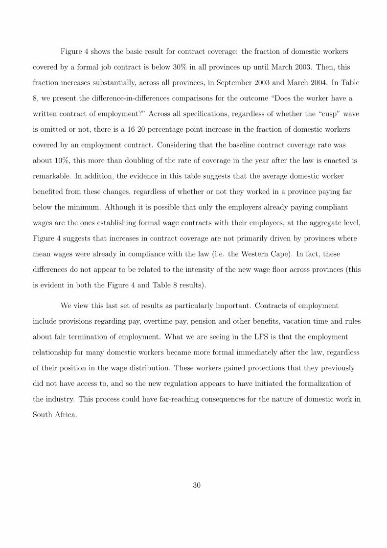
Figure 4 shows the basic result for contract coverage: the fraction of domestic workers

covered by a formal job contract is below 30% in all provinces up until March 2003. Then, this

fraction increases substantially, across all provinces, in September 2003 and March 2004. In Table

8, we present the difference-in-differences comparisons for the outcome “Does the worker have a

written contract of employment?” Across all specifications, regardless of whether the “cusp” wave

is omitted or not, there is a 16-20 percentage point increase in the fraction of domestic workers

covered by an employment contract. Considering that the baseline contract coverage rate was

about 10%, this more than doubling of the rate of coverage in the year after the law is enacted is

remarkable. In addition, the evidence in this table suggests that the average domestic worker

benefited from these changes, regardless of whether or not they worked in a province paying far

below the minimum. Although it is possible that only the employers already paying compliant

wages are the ones establishing formal wage contracts with their employees, at the aggregate level,

Figure 4 suggests that increases in contract coverage are not primarily driven by provinces where

mean wages were already in compliance with the law (i.e. the Western Cape). In fact, these

differences do not appear to be related to the intensity of the new wage floor across provinces (this

is evident in both the Figure 4 and Table 8 results).

We view this last set of results as particularly important. Contracts of employment

include provisions regarding pay, overtime pay, pension and other benefits, vacation time and rules

about fair termination of employment. What we are seeing in the LFS is that the employment

relationship for many domestic workers became more formal immediately after the law, regardless

of their position in the wage distribution. These workers gained protections that they previously

did not have access to, and so the new regulation appears to have initiated the formalization of

the industry. This process could have far-reaching consequences for the nature of domestic work in

South Africa.

30

5 Discussion and conclusions

The introduction of a new minimum wage law in a previously unregulated informal market

presents a unique opportunity to examine important issues around responses to legal wage floors.

It also allows us a window into how informal labor markets operate and the conditions under

which they might formalize.

Although conditions in and characteristics of the domestic worker industry in South

Africa were stable before the introduction of a minimum wage, wages in this sector rose

significantly and substantially – at least 10% compared with other workers – POST -law. When

we consider the difference-in-differences results, it is clear that domestic workers who work in

areas where the pre-law median wage is below the minimum (i.e. where the new law has more

“bite”) experienced even larger increases in wages in the POST -period. Despite the absence of

full compliance and a sharp wage spike at the minimum, we find evidence of a strong wage

response to the law, and little statistical evidence that the law had a negative effect on work on

the intensive or extensive margin. The main purpose of our paper has been to document these

changes and to provide evidence that labor market regulation in an informal sector of considerable

importance can have real impact, even without monitoring or enforcement.

Given that issues of compliance are not often at the center of empirical work on minimum

wages42, it is worthwhile considering how our results should be interpreted. One possible reason

that the law had an effect is that some fraction of employers erroneously believed that the

government was going to enforce the new minimum and penalize non-compliers. A difficulty with

this explanation is that it cannot account for wage or earnings increases for domestic workers

already paid more than the minimum before the law. Although we do not have a panel data set of

workers to test this directly, the fact that the wage and earnings distribution fanned out (the

variance increased) rather than compressing after the law suggests that some employers increased

42For comprehensive reviews of the minimum wage literature, see Brown (1999), Card and Krueger (1997) andNeumark and Wascher (1995, 2007).

31

wages in excess of the minimum, despite already being compliant with the law.

A second reason that an unenforced law may have been effective relates to models of

fairness in wage-setting. A theoretical literature in labor economics posits that the notion of a fair

wage is important in incentivizing workers to provide high effort in tasks for which effort is

unobservable (Akerlof, 1982, 1984 and Akerlof and Yellen, 1988). These models are difficult to

test empirically, since defining and measuring a fair wage, or a reference wage, is tricky in

practice.43 Experimental studies have separately established the importance of gift exchange and

fairness intentions in employer-employee relationships.44 In the case of the domestic worker

industry in South Africa, it is plausible that the announcement of a wage floor defined, or

re-defined, what the fair wage was and set in motion voluntary employer responses, even though

the two traditional channels for encouraging compliance– enforcement and penalties– were closed

off.45 What we take from our analysis is that in the initial stages of labor market formalization,

governments may need to accept partial compliance with new legislation in order to bring about

real changes in outcomes without significant disemployment.46 Even without enforcement, such

legislation can move the market towards a more formal setting, if, for example, it increases

contract coverage, as in the South African case.

We emphasize that our conclusions are valid for the domestic worker industry, which is

one example of an informal sector. The dynamics of the employment relationship between a single

employer and a single employee no doubt condition the response to the law and so may only be

43Mas (2006) is an exception.44See for example Brandts and Charness (2004), who show that a minimum wage may undermine the efficiencies

that gift-exchange can achieve, Falk et al (2000) discuss how fairness intentions matter for behavior and Fehr etal (1997) model how reciprocity in response to fair behavior expands the set of enforceable contracts that can besustained in an economy. Konow (2003) reviews the large body of experimental evidence on fairness. Falk, Fehrand Zehnder (2005) provide a model and experimental evidence that the announcement of a minimum wage raisesworkers’ reservation wages in a persistent way. Reservation wages remain high even after the wage floor is removed,suggesting that policy interventions may have direct and indirect effects on behavior by altering the meaning of afair transaction and by creating ‘entitlement’ effects.

45Rebitzer and Taylor (1995) present a theoretical model of a labor market in which employment increases whenthe minimum wage increases, as a result of an efficiency wage. However, they assume compliance with the law intheir model. They focus on showing how an efficiency wage model can predict an increase in labor demand followinga minimum wage change.

46See Basu, Chau and Kanbur (2007) for a theoretical discussion of why non-compliance with a minimum wagecould be acceptable.

32

relevant in some types of informal enterprizes. However, this characterization of the informal

sector may not be too far from a description of the typical small-scale firm that generates much

informal sector employment in developing countries.47 Also, our analysis is only relevant for the

short-run effects of a new minimum wage policy: while we find clear effects in the 16 months after

the law, as employers face annual increases in this minimum (often above inflation in the case of

South Africa) and as workers sort across space in response to these new protections, the wage,

earnings and employment effects of the policy may change as the sector itself becomes more

formal over time. For example, employers may decide to contract child-care out to day-care

centers which could have feedback effects on equilibrium wages, earnings, hours of work and

number of jobs for domestic workers. We leave questions about the longer-term effects of

formalizing the domestic worker market for future research.

47Banerjee and Duflo (2006)) show that small-scale firms and entrepreneurial activities are an important source ofincome for the poor.

33

References

Akerlof, George, “Labor contracts as partial gift exchange,” Quarterly Journal of Economics,

1982, 97 (4), 543–569.

, “Gift exchange and efficiency-wage theory: Four views,” American Economic Review, 1984,

74 (2), 79–83.

and Janet Yellen, “Fairness and unemployment,” American Economic Review, 1988, 78 (2),

44–49.

Ashenfelter, Orley and Richard Smith, “Compliance with the minimum wage law,” Journal

of Political Economy, April 1979, 2, 333–350.

Banerjee, Abhijit and Esther Duflo, “The economic lives of the poor,” October 2006. Mimeo,

MIT.

Basu, Arnab K., Nancy H. Chau, and Ravi Kanbur, “Turning a blind eye: Costly

enforcement, credible commitment and minimum wage laws,” August 2007. IZA Discussion

Paper No. 2998.

Bell, Linda A., “The impact of minimum wages in Mexico and Colombia,” Journal of Labor

Economics, 1997, (15: 2).

Bertrand, Marianne, Esther Duflo, and Sendhil Mullainathan, “How much should we

trust difference-in-differences estimates?,” Quarterly Journal of Economics, 2004, 119 (1),

249–275.

Besley, Timothy and Robin Burgess, “Can labor regulation hinder economic performance?

Evidence from India,” Quarterly Journal of Economics, 2004.

Bloom, David and Georges Grenier, “Models of Firm Behavior under Minimum Wage

Legislation,” NBER Working Paper, 1986, (1877).

Brandts, Jordi and Gary Charness, “Do labour market conditions affect gift exchange? Some

experimental evidence,” 2004. Universitat Pompeu Fabra Working Paper No. 491.

Branson, Nicola, “Re-weighting the OHS and LFS National Household Survey Data to create a

consistent series over time: A Cross Entropy Estimation Approach,” 2009. SALDRU/DataFirst

34

Working Paper Series number 38.

Brown, Charles, “Minimum wage laws: Are they overrated?,” Journal of Economic

Perspectives, 1988, 2 (3).

, Handbook of Labor Economics, Vol. 3, Elsevier Science, 1999.

Budlender, D., E. Kalula, B. Letsoela, B. Ntshalintshali, and Z. Rustomjee,

“Recommendations of the Employment Conditions Commission on the Investigation into the

Domestic Worker Sector,” Technical Report, South African Department of Labour 2002.

Card, David and Alan Krueger, Myth and Measurement: The New Economics of the

Minimum Wage, Princeton University Press, 1997.

Chang, Yangming, “Noncompliance behavior of risk averse firms under the minimum wage

law,” Public Finance Quarterly, 1992, 20 (3), 390–402.

and Isaac Ehrlich, “On the economics of compliance with the minimum wage law,” Journal

of Political Economy, 1985, 93 (1), 84–91.

Cock, Jacklyn, Maids and madams : Domestic workers under apartheid, London : Women’s

Press, 1989.

Cortes, Kalena, “Wage Effects on Immigrants from an Increase in the Minimum Wage Rate: An

Analysis by Immigrant Industry Concentration,” Working Paper, IZA Discussion Paper No.

1064 2004.

Cortes, Patricia and Jessica Pan, “Outsourcing household production: Foreign domestic

helpers and native labor supply in Hong Kong,” 2009. Mimeo, Chicago Booth School.

DiNardo, John, Nicole Fortin, and Thomas Lemieux, “Labor Market Institutions and the

Distribution of Wages, 1973-1992 : A Semiparametric Analysis,” Econometrica, September

1996, 64, 1001–1044.

Donald, Stephen G. and Kevin Lang, “Inference with difference-in-differences and other

panel data,” Review of Economics and Statistics, 2007, 89 (2), 221–233.

Falk, Armin, Ernst Fehr, and Christian Zehnder, “The behavioral effects of the minimum

wage,” June 2005. IZA Discussion Paper No. 1625.

35

, , and Urs Fischbacher, “Testing Theories of Fairness-Intentions Matter,” 2000.

University of Zurich.

Fehr, Ernst, Simon Gachter, and Georg Kirschteiger, “Reciprocity as a contract

enforcement device: experimental evidence,” Econometrica, 1997, 65 (4).

Gindling, T. H. and Katherine Terrell, “Legal minimum wages and the wages of formal and

informal sector workers in Costa Rica,” February 2004. IZA Discussion Paper No. 1018.

Grenier, Georges, “On compliance with the minimum wage law,” Journal of Political Economy,

1982, 90 (1), 184–187.

Hertz, Tom, “Have minimum wages benefited South Africa’s domestic service workers?,” 2006.

Working Paper, Department of Economics, American University.

Konow, James, “Which is the fairest one of all? A positive analysis of justice theories,” Journal

of Economic Literature, 2003, 41 (4).

Kremer, Michael and Stanley Watt, “The globalization of household production,” September

2006. Mimeo, Harvard University.

Lee, David, “Wage inequality in the United States during the 1980s: Rising dispersion or falling

minimum wage?,” Quarterly Journal of Economics, August 1999, 114 (3), 977–1023.

Lemos, Sara, “Minimum wage effects in a developing country,” Labour Economics, 2009, 16.

Lott, John R. and Russell D. Roberts, “The Expected Penalty for committing a crime: An

Analysis of Minimum Wage Violations,” Journal of Human Resources, 1995, 30 (2), 397–408.

Louw, Megan and Servaas van der Berg, “Labour trends observed in South Africa:

1995-2002,” Technical Report, The World Bank and University of Stellenbosch 2004.

DIFID-WB Collaboration on Knowledge and Skills in the New Economy.

Lustig, Nora and Daniel McLeod, Labor markets in Latin America, Brookings Institution

Press, 1997.

Maloney, W. and J. Menendez, Law and Employment: Lessons from Latin America and the

Caribbean, NBER and University of Chicago, 2004.

Mas, Alex, “Pay, reference points and policy performance,” Quarterly Journal of Economics,

36

August 2006.

Neumark, David and William Wascher, “Minimum Wage Effects on School and Work

Transitions of Teenagers,” American Economic Review Papers and Proceedings, May 1995, 85

(2), 244–49.

and , “Minimum wages and employment,” January 2007. IZA Discussion Paper No. 2570.

Rebitzer, James B. and Lowell J. Taylor, “The consequences of minimum wage laws: Some

new theoretical ideas,” Journal of Public Economics, 1995, 56, 245–255.

Rubinow, I. M., “The problem of domestic service,” Journal of Political Economy, 1906, 14: 8,

502 – 519.

South African Department of Labor, “Labor Relations Act 1995,” Technical Report, South

African Government 1995.

Squire, Lyn and Sethaput Suthiwart-Narueput, “The impact of labor market regulations,”

World Bank Research Observer, 1997, 11 (1), 119–143.

Statistics South Africa, “Labor Force Surveys Waves 4-8,” Technical Report, South African

Government 2000-2003.

, “Income and Expenditure Surveys 2000 and 2005,” Technical Report, South African

Government 2000, 2005.

Thiess, Clifford F., “The first minimum wage laws,” CATO Journal, 1991, Winter (10).

Weil, David, “Public Enforcement/Private Monitoring: Evaluating a new approach to regulating

the minimum wage,” Industrial and Labor Relations Review, January 2005, 58.

37

Figure 1: Distribution of log hourly wages for urban domestic workers

Figure 2: Distribution of log monthly earnings for urban domestic workers

Kernel density plots of log hourly wages (bandwidth 0.02) and log monthly earnings (bandwidth 0.08). Data are from South AfricanLabor Force Surveys (March 2001-March 2004). The vertical line is at the level of the full-time minimum wage (monthly income) forurban domestic workers. Each wave of data contains between 996 and 1,260 observations. Kolmogorov-Smirnov tests of equality ofdistributions reject at the 5% level for each pairwise comparison of waves in the before and after periods.

38

Figure 3: Mean hourly domestic worker wages by province over time

Each dot represents a province-wave level mean hourly wage for domestic workers, for waves before and after the law. The black verticaldashed lines demarcate the period before (to the left) and the period after (to the right) the law, with the “cusp” period falling betweenthese lines. The red horizontal dashed line represents the urban full-time minimum wage (ZAR4.1) established in November 2002. Alldata are from the South African Labor Force Surveys (March 2001-March 2004) and means are weighted. Provinces are: Western Cape(WC), Eastern Cape (EC), Northern Cape (NC), Free State (FS), Kwazulu-Natal (KZN), Northern Province (NP), Gauteng (Gau),Mpumalanga (MP) and Limpopo (LIM).

39

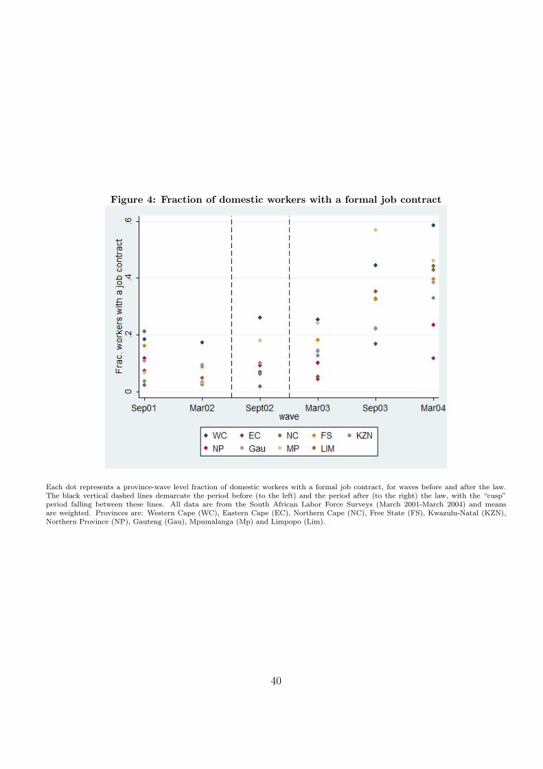
Figure 4: Fraction of domestic workers with a formal job contract

Each dot represents a province-wave level fraction of domestic workers with a formal job contract, for waves before and after the law.The black vertical dashed lines demarcate the period before (to the left) and the period after (to the right) the law, with the “cusp”period falling between these lines. All data are from the South African Labor Force Surveys (March 2001-March 2004) and meansare weighted. Provinces are: Western Cape (WC), Eastern Cape (EC), Northern Cape (NC), Free State (FS), Kwazulu-Natal (KZN),Northern Province (NP), Gauteng (Gau), Mpumalanga (Mp) and Limpopo (Lim).

40

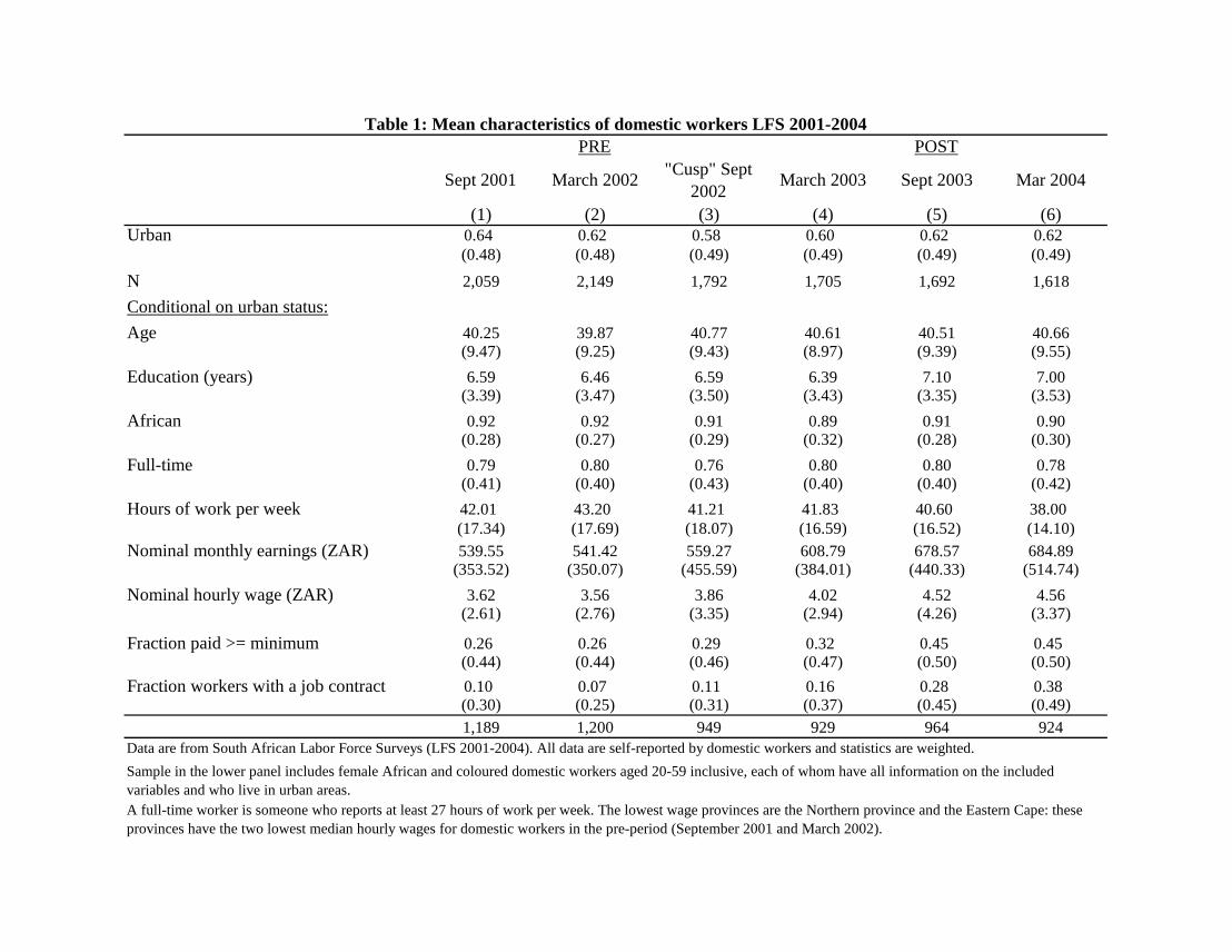
(1) (2) (3) (4) (5) (6)Urban 0.64 0.62 0.58 0.60 0.62 0.62

(0.48) (0.48) (0.49) (0.49) (0.49) (0.49)

N 2,059 2,149 1,792 1,705 1,692 1,618Conditional on urban status:Age 40.25 39.87 40.77 40.61 40.51 40.66

(9.47) (9.25) (9.43) (8.97) (9.39) (9.55)Education (years) 6.59 6.46 6.59 6.39 7.10 7.00

(3.39) (3.47) (3.50) (3.43) (3.35) (3.53)African 0.92 0.92 0.91 0.89 0.91 0.90

(0.28) (0.27) (0.29) (0.32) (0.28) (0.30)Full-time 0.79 0.80 0.76 0.80 0.80 0.78

(0.41) (0.40) (0.43) (0.40) (0.40) (0.42)Hours of work per week 42.01 43.20 41.21 41.83 40.60 38.00

(17.34) (17.69) (18.07) (16.59) (16.52) (14.10)Nominal monthly earnings (ZAR) 539.55 541.42 559.27 608.79 678.57 684.89

(353.52) (350.07) (455.59) (384.01) (440.33) (514.74)Nominal hourly wage (ZAR) 3.62 3.56 3.86 4.02 4.52 4.56

(2.61) (2.76) (3.35) (2.94) (4.26) (3.37)

Fraction paid >= minimum 0.26 0.26 0.29 0.32 0.45 0.45(0.44) (0.44) (0.46) (0.47) (0.50) (0.50)

Fraction workers with a job contract 0.10 0.07 0.11 0.16 0.28 0.38(0.30) (0.25) (0.31) (0.37) (0.45) (0.49)

1,189 1,200 949 929 964 924

Table 1: Mean characteristics of domestic workers LFS 2001-2004

Data are from South African Labor Force Surveys (LFS 2001-2004). All data are self-reported by domestic workers and statistics are weighted.Sample in the lower panel includes female African and coloured domestic workers aged 20-59 inclusive, each of whom have all information on the included variables and who live in urban areas.A full-time worker is someone who reports at least 27 hours of work per week. The lowest wage provinces are the Northern province and the Eastern Cape: these provinces have the two lowest median hourly wages for domestic workers in the pre-period (September 2001 and March 2002).

POSTPRE

Sept 2001 March 2002 March 2003 Sept 2003 Mar 2004"Cusp" Sept 2002

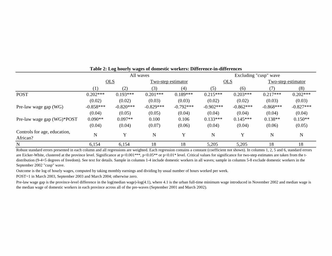
(1) (2) (3) (4) (5) (6) (7) (8)POST 0.202*** 0.193*** 0.201*** 0.189*** 0.215*** 0.203*** 0.217*** 0.202***

(0.02) (0.02) (0.03) (0.03) (0.02) (0.02) (0.03) (0.03)Pre-law wage gap (WG) -0.858*** -0.820*** -0.829*** -0.792*** -0.902*** -0.862*** -0.868*** -0.827***

(0.04) (0.05) (0.05) (0.04) (0.04) (0.04) (0.04) (0.04)Pre-law wage gap (WG)*POST 0.090** 0.097** 0.100 0.106 0.133*** 0.145*** 0.138** 0.150**

(0.04) (0.04) (0.07) (0.06) (0.04) (0.04) (0.06) (0.05)Controls for age, education, African? N Y N Y N Y N N

N 6,154 6,154 18 18 5,205 5,205 18 18

Outcome is the log of hourly wages, computed by taking monthly earnings and dividing by usual number of hours worked per week.POST=1 in March 2003, September 2003 and March 2004; otherwise zero.

Table 2: Log hourly wages of domestic workers: Difference-in-differences

Robust standard errors presented in each column and all regressions are weighted. Each regression contains a constant (coefficient not shown). In columns 1, 2, 5 and 6, standard errors are Eicker-White, clustered at the province level. Significance at p<0.001***, p<0.05** or p<0.01* level. Critical values for significance for two-step estimates are taken from the t-distribution (9-4=5 degrees of freedom). See text for details. Sample in columns 1-4 include domestic workers in all waves; sample in columns 5-8 exclude domestic workers in the September 2002 "cusp" wave.

Pre-law wage gap is the province-level difference in the log(median wage)-log(4.1), where 4.1 is the urban full-time minimum wage introduced in November 2002 and median wage is the median wage of domestic workers in each province across all of the pre-waves (September 2001 and March 2002).

OLSOLS Two-step estimatorAll waves Excluding "cusp" wave

Two-step estimator

(1) (2) (3) (4) (5) (6) (7) (8)POST -0.887 -0.901 -0.848 -0.761 -1.149 -1.111 -0.874 -0.77

(0.82) (0.81) (1.58) (1.39) (1.18) (1.14) (1.62) (1.40)Pre-law wage gap (WG) 5.151 3.98 5.758** 4.996** 5.383 4.1 6.675** 5.729**

(3.21) (2.58) (2.52) (2.17) (3.84) (3.01) (2.94) (2.48)Pre-law wage gap (WG)*POST -2.832 -3.309 -4.157 -4.283 -3.064 -3.579 -5.074 -5.128

(2.17) (2.28) (3.79) (3.50) (3.20) (3.23) (4.08) (3.70)Controls for age, education, African? N Y N Y N Y N Y

N 6,876 6,876 18 18 5,824 5,824 18 18

Outcome is usual number of hours worked per week.POST=1 in March 2003, September 2003 and March 2004; otherwise zero.

Robust standard errors presented in each column and all regressions are weighted. Each regression contains a constant (coefficient not shown). In columns 1, 2, 5 and 6, standard errors are Eicker-White, clustered at the province level. Significance at p<0.001***, p<0.05** or p<0.01* level. Critical values for significance for two-step estimates are taken from the t-distribution (9-4=5 degrees of freedom). See text for details. Sample in columns 1-4 include domestic workers in all waves; sample in columns 5-8 exclude domestic workers in the September 2002 "cusp" wave.

Pre-law wage gap is the province-level difference in the log(median wage)-log(4.1), where 4.1 is the urban full-time minimum wage introduced in November 2002 and median wage is the median wage of domestic workers in each province across all of the pre-waves (September 2001 and March 2002).

Table 3: Usual weekly hours of work of domestic workers: Difference-in-differencesAll waves Excluding "cusp" wave

OLS Two-step estimator OLS Two-step estimator

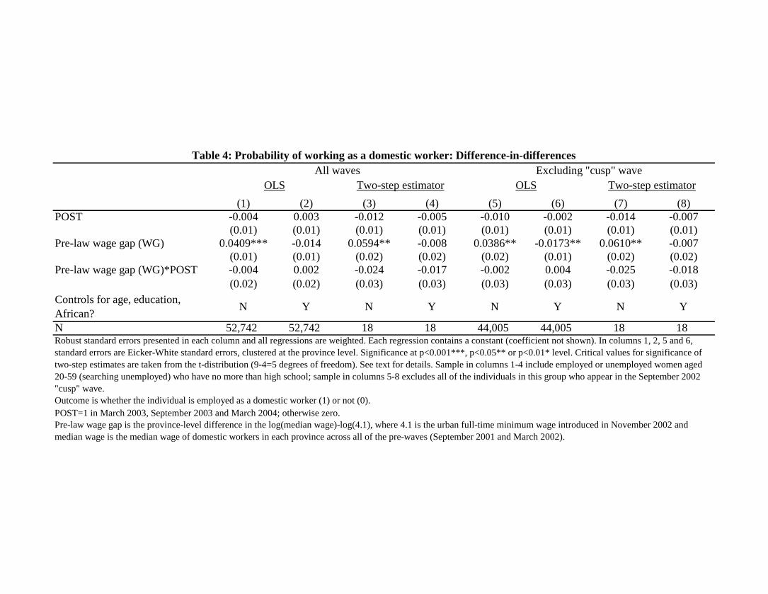
(1) (2) (3) (4) (5) (6) (7) (8)POST -0.004 0.003 -0.012 -0.005 -0.010 -0.002 -0.014 -0.007

(0.01) (0.01) (0.01) (0.01) (0.01) (0.01) (0.01) (0.01)Pre-law wage gap (WG) 0.0409*** -0.014 0.0594** -0.008 0.0386** -0.0173** 0.0610** -0.007

(0.01) (0.01) (0.02) (0.02) (0.02) (0.01) (0.02) (0.02)Pre-law wage gap (WG)*POST -0.004 0.002 -0.024 -0.017 -0.002 0.004 -0.025 -0.018

(0.02) (0.02) (0.03) (0.03) (0.03) (0.03) (0.03) (0.03)Controls for age, education, African? N Y N Y N Y N Y

N 52,742 52,742 18 18 44,005 44,005 18 18

Outcome is whether the individual is employed as a domestic worker (1) or not (0).POST=1 in March 2003, September 2003 and March 2004; otherwise zero.

Robust standard errors presented in each column and all regressions are weighted. Each regression contains a constant (coefficient not shown). In columns 1, 2, 5 and 6, standard errors are Eicker-White standard errors, clustered at the province level. Significance at p<0.001***, p<0.05** or p<0.01* level. Critical values for significance of two-step estimates are taken from the t-distribution (9-4=5 degrees of freedom). See text for details. Sample in columns 1-4 include employed or unemployed women aged 20-59 (searching unemployed) who have no more than high school; sample in columns 5-8 excludes all of the individuals in this group who appear in the September 2002 "cusp" wave.

Pre-law wage gap is the province-level difference in the log(median wage)-log(4.1), where 4.1 is the urban full-time minimum wage introduced in November 2002 and median wage is the median wage of domestic workers in each province across all of the pre-waves (September 2001 and March 2002).

Table 4: Probability of working as a domestic worker: Difference-in-differencesAll waves Excluding "cusp" wave

OLS Two-step estimator OLS Two-step estimator

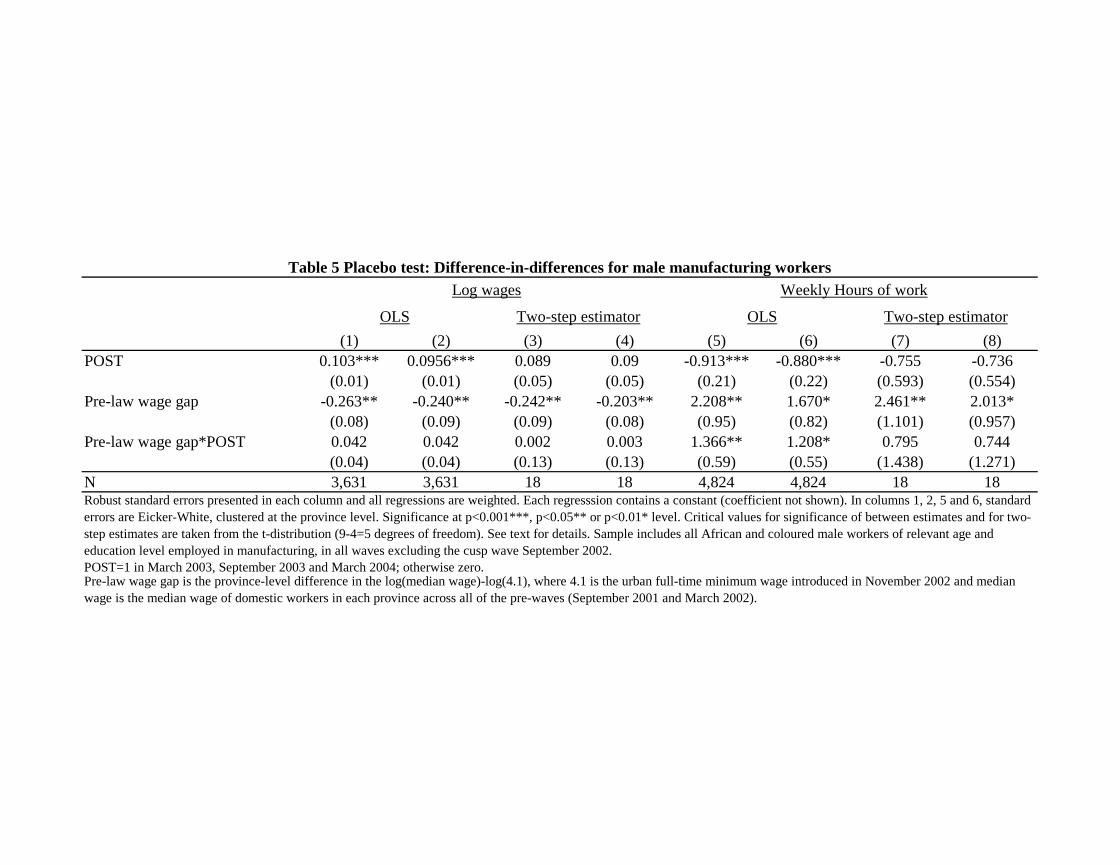
(1) (2) (3) (4) (5) (6) (7) (8)POST 0.103*** 0.0956*** 0.089 0.09 -0.913*** -0.880*** -0.755 -0.736

(0.01) (0.01) (0.05) (0.05) (0.21) (0.22) (0.593) (0.554)Pre-law wage gap -0.263** -0.240** -0.242** -0.203** 2.208** 1.670* 2.461** 2.013*

(0.08) (0.09) (0.09) (0.08) (0.95) (0.82) (1.101) (0.957)Pre-law wage gap*POST 0.042 0.042 0.002 0.003 1.366** 1.208* 0.795 0.744

(0.04) (0.04) (0.13) (0.13) (0.59) (0.55) (1.438) (1.271)N 3,631 3,631 18 18 4,824 4,824 18 18

POST=1 in March 2003, September 2003 and March 2004; otherwise zero.

Table 5 Placebo test: Difference-in-differences for male manufacturing workers

Robust standard errors presented in each column and all regressions are weighted. Each regresssion contains a constant (coefficient not shown). In columns 1, 2, 5 and 6, standard errors are Eicker-White, clustered at the province level. Significance at p<0.001***, p<0.05** or p<0.01* level. Critical values for significance of between estimates and for two-step estimates are taken from the t-distribution (9-4=5 degrees of freedom). See text for details. Sample includes all African and coloured male workers of relevant age and education level employed in manufacturing, in all waves excluding the cusp wave September 2002.

Pre-law wage gap is the province-level difference in the log(median wage)-log(4.1), where 4.1 is the urban full-time minimum wage introduced in November 2002 and median wage is the median wage of domestic workers in each province across all of the pre-waves (September 2001 and March 2002).

OLS Two-step estimator

Log wages Weekly Hours of work

OLS Two-step estimator

δ1=0.8*wmin δ1=0.8*wmin

No controls All controls All controls No controls All controls All controls

(1) (2) (3) (4) (5) (6)Change in fraction with non-compliant wagesPr(w*=0|POST)-Pr(w*=0|PRE) -0.149*** -0.139*** -0.147*** -0.141*** -0.134*** -0.141***

(0.016) (0.016) (0.016) (0.026) (0.026) (0.026)Change in fraction with near-compliant wagesPr(w*=1|POST)-Pr(w*=1|PRE) 0.007*** 0.007*** 0.012*** 0.008*** 0.008*** 0.010***

(0.001) (0.001) (0.002) (0.002) (0.002) (0.002)Change in fraction with compliant wagePr(w*=2|POST)-Pr(w*=2|PRE) 0.142*** 0.132*** 0.138*** 0.133*** 0.127*** 0.131***

(0.015) (0.015) (0.015) (0.025) (0.025) (0.024)

Change in fraction with non-compliant wagesPr(w*=0|POST*WG)-Pr(w*=0|PRE*WG) -0.077 -0.084* -0.085*

(0.051) (0.051) (0.050)Change in fraction with near-compliant wagesPr(w*=1|POST*WG)-Pr(w*=1|PRE*WG) 0.004 0.004 0.005

(0.003) (0.003) (0.003)Change in fraction with compliant wagePr(w*=2|POST*WG)-Pr(w*=2|PRE*WG) 0.073 0.080* 0.080*

(0.048) (0.048) (0.047)

N workers 5,206 5,206 5,206 5,206 5,206 5,206Robust standard errors in parentheses. Significant at p<0.001***, p<0.05** or p<0.01* level. All regressions weighted.

Each specification includes a constant and an indicator for whether the observation is captured PRE or POST law. Columns (2) and (3), (5) and (6) present results from models which control for age, race, years of education. Columns (4), (5) and (6) present results from the specification that controls for a POST indicator, a measure of the log wage gap in the province before the law was in effect, and the interaction of POST with wage gap (WG). The estimates in the lower panel of columns (4)-(6) are the coefficients and standard errors on the interaction of POST*WG.

Sample restricted to urban female domestic workers ages 20-59 in pre- and post-periods (Sep 01-Mar 04), excluding the cusp wave (September 2002).

δ1=0.9*wmin δ1=0.9*wmin

Results are predicted changes in the probability of falling into one of three groups generated from an ordered probit model. The three groups are: non-compliant (w=0), near-compliant (w=1) and compliant (w=2). The near-compliant group is defined as the set of wages 10% below the minimum or less; 20% below the minimum or less in each of columns (1-2) and (3). Marginal effects are calculated using STATA's mfx command, which computes the "effect" of switching a binary variable from 0 to 1.

Table 6: Testing for partial compliance in response to the law: Marginal effects from ordered probit

Average change in predicted probability of domestic worker reporting nominal wages in the non-compliant, near-compliant or compliant region

Before-After comparison Before-After comparison by intensity of the law

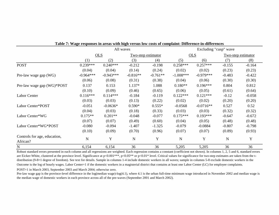
(1) (2) (3) (4) (5) (6) (7) (8)POST 0.239*** 0.240*** -0.212 -0.198 0.258*** 0.257*** -0.155 -0.164

(0.04) (0.04) (0.14) (0.24) (0.02) (0.02) (0.23) (0.23)Pre-law wage gap (WG) -0.964*** -0.943*** -0.816** -0.761** -1.008*** -0.979*** -0.483 -0.422

(0.06) (0.08) (0.31) (0.38) (0.04) (0.06) (0.30) (0.30)Pre-law wage gap (WG)*POST 0.137 0.153 1.137* 1.088 0.180** 0.196*** 0.804 0.812

(0.10) (0.09) (0.46) (0.65) (0.06) (0.05) (0.61) (0.64)Labor Center 0.116*** 0.114*** -0.184 -0.119 0.122*** 0.121*** -0.12 -0.058

(0.03) (0.03) (0.13) (0.22) (0.02) (0.02) (0.20) (0.20)Labor Center*POST -0.051 -0.0636* 0.590* 0.555* -0.0568 -0.0716** 0.527 0.52

(0.04) (0.03) (0.18) (0.33) (0.03) (0.03) (0.32) (0.32)Labor Center*WG 0.175** 0.201** -0.048 -0.077 0.175*** 0.193*** -0.647 -0.672

(0.07) (0.07) (0.49) (0.60) (0.04) (0.05) (0.48) (0.48)Labor Center*WG*POST -0.080 -0.094 -1.407 -1.325 -0.079 -0.0884 -0.807 -0.798

(0.10) (0.09) (0.70) (0.96) (0.07) (0.07) (0.89) (0.93)Controls for age, education, African? N Y N Y N Y N Y

N 6,154 6,154 36 36 5,205 5,205 36 36

POST=1 in March 2003, September 2003 and March 2004; otherwise zero.

Table 7: Wage responses in areas with high versus low costs of complaint: Difference-in-differencesAll waves Excluding "cusp" wave

OLS Two-step estimator OLS Two-step estimator

Robust standard errors presented in each column and all regressions are weighted. Each regression contains a constant (coefficient not shown). In columns 1, 2, 5 and 6, standard errors are Eicker-White, clustered at the province level. Significance at p<0.001***, p<0.05** or p<0.01* level. Critical values for significance for two-step estimates are taken from the t-distribution (9-8=1 degree of freedom). See text for details. Sample in columns 1-4 include domestic workers in all waves; sample in columns 5-8 exclude domestic workers in the

Pre-law wage gap is the province-level difference in the log(median wage)-log(4.1), where 4.1 is the urban full-time minimum wage introduced in November 2002 and median wage is the median wage of domestic workers in each province across all of the pre-waves (September 2001 and March 2002).

Outcome is the log of hourly wages. Labor Center=1 if the domestic workers in a magisterial district that contains at least one Labor Center (LC) for employee complaints.

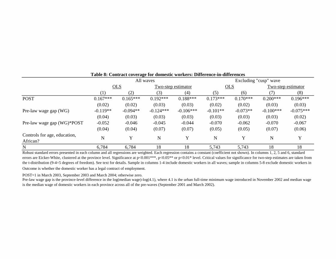
(1) (2) (3) (4) (5) (6) (7) (8)POST 0.167*** 0.165*** 0.192*** 0.188*** 0.173*** 0.170*** 0.200*** 0.196***

(0.02) (0.02) (0.03) (0.03) (0.02) (0.02) (0.03) (0.03)Pre-law wage gap (WG) -0.119** -0.094** -0.124*** -0.106*** -0.101** -0.073** -0.100*** -0.075***

(0.04) (0.03) (0.03) (0.03) (0.03) (0.03) (0.03) (0.02)Pre-law wage gap (WG)*POST -0.052 -0.046 -0.045 -0.044 -0.070 -0.062 -0.070 -0.067

(0.04) (0.04) (0.07) (0.07) (0.05) (0.05) (0.07) (0.06)Controls for age, education, African? N Y N Y N Y N Y

N 6,784 6,784 18 18 5,743 5,743 18 18

Outcome is whether the domestic worker has a legal contract of employment.

POST=1 in March 2003, September 2003 and March 2004; otherwise zero.

Robust standard errors presented in each column and all regressions are weighted. Each regression contains a constant (coefficient not shown). In columns 1, 2, 5 and 6, standard errors are Eicker-White, clustered at the province level. Significance at p<0.001***, p<0.05** or p<0.01* level. Critical values for significance for two-step estimates are taken from the t-distribution (9-4=5 degrees of freedom). See text for details. Sample in columns 1-4 include domestic workers in all waves; sample in columns 5-8 exclude domestic workers in

Pre-law wage gap is the province-level difference in the log(median wage)-log(4.1), where 4.1 is the urban full-time minimum wage introduced in November 2002 and median wage is the median wage of domestic workers in each province across all of the pre-waves (September 2001 and March 2002).

Table 8: Contract coverage for domestic workers: Difference-in-differencesAll waves Excluding "cusp" wave

OLS Two-step estimator OLS Two-step estimator

Appendix 1: Testing for evidence of incomplete wage

adjustment

Consider the figure below which shows the wage distribution F(.) of domestic worker wages in theperiod before and after the law. FAfter is shifted to the right of FBefore and the solid black verticalline at δ2 represents the minimum wage level. Define δ1 as 90% of the minimum wage. Then,classify all worker wages into one of three groups: wages below δ1 are non-compliant, wagesbetween δ1 and δ2 are nearly compliant, and wages at or above δ2 are compliant.

We would like to know whether the shift in the wage distribution in response to the law isconsistent with incomplete adjustment up to compliant levels. That is, are wages shifting up outof the bottom part of the distribution, but not enough to get most workers up to or over theminimum threshold? Some shifts in the distribution are consistent with this idea and some arenot. In example 1 below, the first set of changes in the fraction of workers in each region would beconsistent with complete adjustment for some workers up to compliance: 10% of workers in eachof the non-compliant and near-compliant regions leave these regions; and 20% of workers join thecompliant region. The second example is, however, not consistent with full compliance for workerswho experience wage changes: 20% of workers leave the non-compliant region, and thenear-compliant region grows by 10% of workers as does the compliant region. While we cannot saywhich exact workers are getting wage increase, as long as jobs are not being lost as a result of thelaw change, then such shifts in the overall distribution reflect partial adjustments in response tothe law.

Example 1Non-compliant region Near compliant Compliant

Before 0.3 0.3 0.4After 0.2 0.2 0.6

Example 2Non-compliant region Near compliant Compliant

Before 0.3 0.3 0.4After 0.1 0.4 0.5

Intuitively, we would like to know whether or not the fall in the fraction of domesticworkers in the non-compliant region is fully offset by the increase in fraction of workers in thecompliant region. We do this by implementing an ordered probit model and testing a specifichypothesis. To describe the appropriate hypothesis, consider the following linear model of the logof the individual worker’s wage (wi) (ignoring covariates for now) where εi ∼ N(0, 1):wi = β0 + tβ1 + εi, where t = 1 if the worker is observed in the after period and t = 0 if observedin the before period. We define an ordered categorical variable, w∗

i that captures the region thateach wage falls into:

w∗i = 0 if wi ≤ δ1 (1)

A test for partial compliance

w∗i = 1 if δ1 < wi ≤ δ2 (2)

w∗i = 2 if wi > δ2 (3)

Then, the probability that any worker’s wage falls into a particular bin can be describedas:

Pr(w∗i = 0) = Pr(wi ≤ δ1) = Pr(β0 + tβ1 + εi ≤ δ1) = Φ(δ1 − β0 − tβ1) (4)

Pr(w∗i = 1) = Pr(δ1 < β0 + tβ1 + εi ≤ δ2) = Φ(δ2 − β0 − tβ1)− Φ(δ1 − β0 − tβ1) (5)

Pr(w∗i = 2) = Pr(β0 + tβ1 + εi ≥ δ2) = 1− Pr(β0 + tβ1 + εi ≤ δ2) = 1− Φ(δ2 − β0 − tβ1) (6)

The hypothesis we would like to test is the following:

H0 :∂Pr(w∗

i = 2)

∂t+∂Pr(w∗

i = 0)

∂t≥ 0 (7)

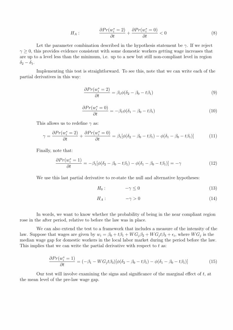
HA :∂Pr(w∗

i = 2)

∂t+∂Pr(w∗

i = 0)

∂t< 0 (8)

Let the parameter combination described in the hypothesis statement be γ. If we rejectγ ≥ 0, this provides evidence consistent with some domestic workers getting wage increases thatare up to a level less than the minimum, i.e. up to a new but still non-compliant level in regionδ2 − δ1.

Implementing this test is straightforward. To see this, note that we can write each of thepartial derivatives in this way:

∂Pr(w∗i = 2)

∂t= β1φ(δ2 − β0 − tβ1) (9)

∂Pr(w∗i = 0)

∂t= −β1φ(δ1 − β0 − tβ1) (10)

This allows us to redefine γ as:

γ =∂Pr(w∗

i = 2)

∂t+∂Pr(w∗

i = 0)

∂t= β1[φ(δ2 − β0 − tβ1)− φ(δ1 − β0 − tβ1)] (11)

Finally, note that:

∂Pr(w∗i = 1)

∂t= −β1[φ(δ2 − β0 − tβ1)− φ(δ1 − β0 − tβ1)] = −γ (12)

We use this last partial derivative to re-state the null and alternative hypotheses:

H0 : −γ ≤ 0 (13)

HA : −γ > 0 (14)

In words, we want to know whether the probability of being in the near compliant regionrose in the after period, relative to before the law was in place.

We can also extend the test to a framework that includes a measure of the intensity of thelaw. Suppose that wages are given by wi = β0 + tβ1 +WGjβ2 +WGjtβ3 + εi, where WGj is themedian wage gap for domestic workers in the local labor market during the period before the law.This implies that we can write the partial derivative with respect to t as:

∂Pr(w∗i = 1)

∂t= (−β1 −WGjtβ3)[φ(δ2 − β0 − tβ1)− φ(δ1 − β0 − tβ1)] (15)

Our test will involve examining the signs and significance of the marginal effect of t, atthe mean level of the pre-law wage gap.

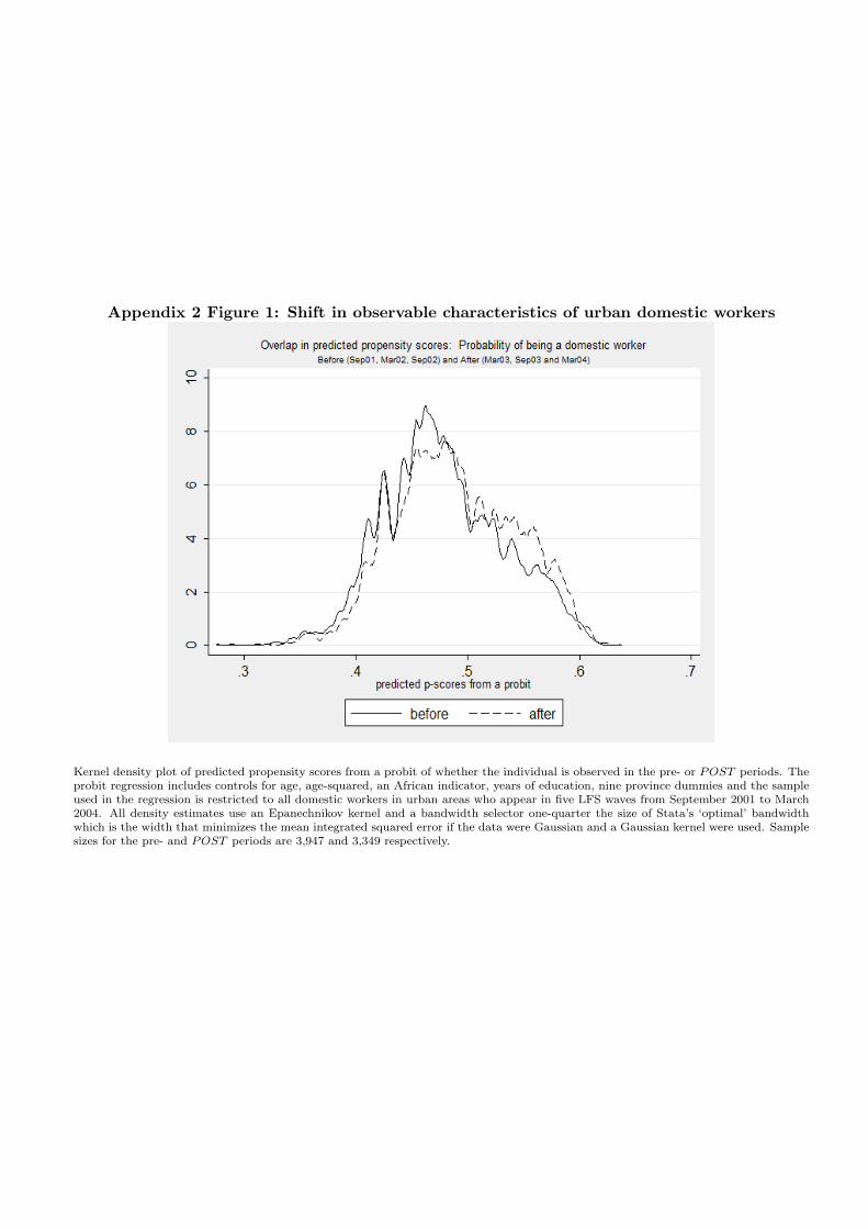
Appendix 2 Figure 1: Shift in observable characteristics of urban domestic workers

Kernel density plot of predicted propensity scores from a probit of whether the individual is observed in the pre- or POST periods. Theprobit regression includes controls for age, age-squared, an African indicator, years of education, nine province dummies and the sampleused in the regression is restricted to all domestic workers in urban areas who appear in five LFS waves from September 2001 to March2004. All density estimates use an Epanechnikov kernel and a bandwidth selector one-quarter the size of Stata’s ‘optimal’ bandwidthwhich is the width that minimizes the mean integrated squared error if the data were Gaussian and a Gaussian kernel were used. Samplesizes for the pre- and POST periods are 3,947 and 3,349 respectively.

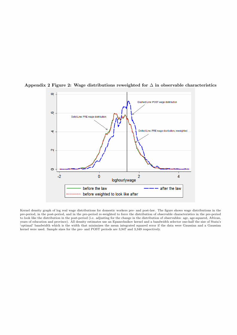
Appendix 2 Figure 2: Wage distributions reweighted for ∆ in observable characteristics

Kernel density graph of log real wage distributions for domestic workers pre- and post-law. The figure shows wage distributions in thepre-period, in the post-period, and in the pre-period re-weighted to force the distribution of observable characteristics in the pre-periodto look like the distribution in the post-period (i.e. adjusting for the change in the distribution of observables: age, age-squared, African,years of education and province). All density estimates use an Epanechnikov kernel and a bandwidth selector one-half the size of Stata’s‘optimal’ bandwidth which is the width that minimizes the mean integrated squared error if the data were Gaussian and a Gaussiankernel were used. Sample sizes for the pre- and POST periods are 3,947 and 3,349 respectively.

(1) (2) (3) (4) (5) (6) (7) (8)POST 0.198*** 0.188*** 0.194*** 0.183*** 0.209*** 0.197*** 0.209*** 0.197***

(0.01) (0.01) (0.03) (0.03) (0.01) (0.01) (0.03) (0.03)Pre-law wage gap (WG) -0.829*** -0.808*** -0.808*** -0.787*** -0.874*** -0.850*** -0.848*** -0.822***

(0.05) (0.05) (0.05) (0.04) (0.05) (0.05) (0.04) (0.04)Pre-law wage gap (WG)*POST 0.109*** 0.111*** 0.102 0.103* 0.154*** 0.157*** 0.142** 0.147**

(0.03) (0.03) (0.07) (0.06) (0.03) (0.03) (0.06) (0.06)Controls for age, education, African? N Y N Y N Y N N

N 6,154 6,154 18 18 5,205 5,205 18 18

Outcome is the log of hourly wages, computed by taking monthly earnings and dividing by usual number of hours worked per week.POST=1 in March 2003, September 2003 and March 2004; otherwise zero.

Appendix 3 Table 1: Log hourly wages of domestic workers: Difference-in-differences, unweighted

Robust standard errors presented in each column. In columns 1, 2, 5 and 6, standard errors are Eicker-White, clustered at the province level. Significance at p<0.001***, p<0.05** or p<0.01* level. Critical values for significance for two-step estimates are taken from the t-distribution (9-4=5 degrees of freedom). See text for details. Sample in columns 1-4 include domestic workers in all waves; sample in columns 5-8 exclude domestic workers in the September 2002 "cusp" wave.

Pre-law wage gap is the province-level difference in the log(median wage)-log(4.1), where 4.1 is the urban full-time minimum wage introduced in November 2002 and median wage is the median wage of domestic workers in each province across all of the pre-waves (September 2001 and March 2002).

OLSOLS Two-step estimatorAll waves Excluding "cusp" wave

Two-step estimator

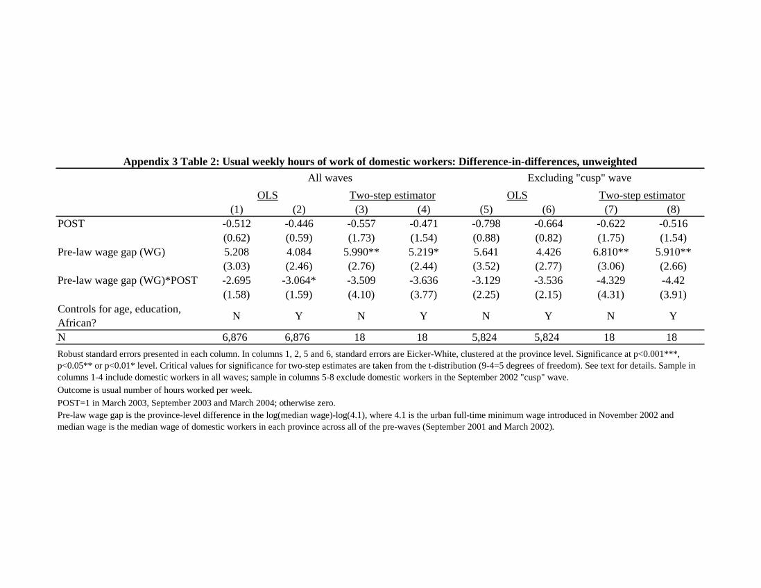
(1) (2) (3) (4) (5) (6) (7) (8)POST -0.512 -0.446 -0.557 -0.471 -0.798 -0.664 -0.622 -0.516

(0.62) (0.59) (1.73) (1.54) (0.88) (0.82) (1.75) (1.54)Pre-law wage gap (WG) 5.208 4.084 5.990** 5.219* 5.641 4.426 6.810** 5.910**

(3.03) (2.46) (2.76) (2.44) (3.52) (2.77) (3.06) (2.66)Pre-law wage gap (WG)*POST -2.695 -3.064* -3.509 -3.636 -3.129 -3.536 -4.329 -4.42

(1.58) (1.59) (4.10) (3.77) (2.25) (2.15) (4.31) (3.91)Controls for age, education, African? N Y N Y N Y N Y

N 6,876 6,876 18 18 5,824 5,824 18 18

Outcome is usual number of hours worked per week.POST=1 in March 2003, September 2003 and March 2004; otherwise zero.

Robust standard errors presented in each column. In columns 1, 2, 5 and 6, standard errors are Eicker-White, clustered at the province level. Significance at p<0.001***, p<0.05** or p<0.01* level. Critical values for significance for two-step estimates are taken from the t-distribution (9-4=5 degrees of freedom). See text for details. Sample in columns 1-4 include domestic workers in all waves; sample in columns 5-8 exclude domestic workers in the September 2002 "cusp" wave.

Pre-law wage gap is the province-level difference in the log(median wage)-log(4.1), where 4.1 is the urban full-time minimum wage introduced in November 2002 and median wage is the median wage of domestic workers in each province across all of the pre-waves (September 2001 and March 2002).

Appendix 3 Table 2: Usual weekly hours of work of domestic workers: Difference-in-differences, unweightedAll waves Excluding "cusp" wave

OLS Two-step estimator OLS Two-step estimator

The Southern Africa Labour and Development Research UnitThe Southern Africa Labour and Development Research Unit (SALDRU) conducts research directed at improving the well-being of South Africa’s poor. It was established in 1975. Over the next two decades the unit’s research played a central role in documenting the human costs of apartheid. Key projects from this period included the Farm Labour Conference (1976), the Economics of Health Care Conference (1978), and the Second Carnegie Enquiry into Poverty and Development in South Africa (1983-86). At the urging of the African Na-tional Congress, from 1992-1994 SALDRU and the World Bank coordinated the Project for Statistics on Living Standards and Development (PSLSD). This project provide baseline data for the implementation of post-apartheid socio-economic policies through South Africa’s first non-racial national sample survey. In the post-apartheid period, SALDRU has continued to gather data and conduct research directed at informing and assessing anti-poverty policy. In line with its historical contribution, SALDRU’s researchers continue to conduct research detailing changing patterns of well-being in South Africa and assessing the impact of government policy on the poor. Current research work falls into the following research themes: post-apartheid poverty; employment and migration dynamics; family support structures in an era of rapid social change; public works and public infrastructure programmes, financial strategies of the poor; common prop-erty resources and the poor. Key survey projects include the Langeberg Integrated Family Survey (1999), the Khayelitsha/Mitchell’s Plain Survey (2000), the ongoing Cape Area Panel Study (2001-) and the Financial Diaries Project.

Southern Africa Labour and Development Research UnitSchool of Economics

University of Cape TownPrivate Bag, Rondebosch, 7701

Cape Town, South Africa

Tel: +27 (0) 21 650 5696Fax: +27 (0) 21 650 5697

Email: brenda.adams@.uct.ac.zaWeb: www.saldru.uct.ac.za

School of EconomicsUNIVERSITY OF C A P E T O W N

SALDRU