Climatic ChangeDOI 10.1007/s10584-011-0023-y

The identification of distinct patterns in Californiatemperature trends

Eugene C. Cordero · Wittaya Kessomkiat ·John Abatzoglou · Steven A. Mauget

Received: 28 August 2009 / Accepted: 4 November 2010© Springer Science+Business Media B.V. 2011

Abstract Regional changes in California surface temperatures over the last 80 yearsare analyzed using station data from the US Historical Climate Network and theNational Weather Service Cooperative Network. Statistical analyses using annualand seasonal temperature data over the last 80 years show distinctly different spatialand temporal patterns in trends of maximum temperature (Tmax) compared totrends of minimum temperature (Tmin). For trends computed between 1918 and2006, the rate of warming in Tmin is greater than that of Tmax. Trends computedsince 1970 show an amplified warming rate compared to trends computed from 1918,and the rate of warming is comparable between Tmin and Tmax. This is especiallytrue in the southern deserts, where warming trends during spring (March–May) areexceptionally large. While observations show coherent statewide positive trends inTmin, trends in Tmax vary on finer spatial and temporal scales. Accompanying theobserved statewide warming from 1970 to 2006, regional cooling trends in Tmaxare observed during winter and summer. These signatures of regional tempera-ture change suggest that a collection of different forcing mechanisms or feedbackprocesses must be present to produce these responses.

E. C. Cordero (B) · W. KessomkiatDepartment of Meteorology and Climate Science, San José State University,San José, CA 95192-0104, USAe-mail: cordero@met.sjsu.edu

J. AbatzoglouDepartment of Geography, University of Idaho, Moscow, ID 83844-3021, USA

S. A. MaugetU.S. Department of Agriculture-Agricultural Research Service, USDA Plant Stress and WaterConservation Laboratory, Lubbock, TX 79415, USA

Climatic Change

1 Introduction

Global average surface temperatures have increased +0.74◦C ± 0.18◦C between1906–2005 (e.g., IPCC 2007). Variations in interannual to multi-decadal tempera-tures are important to understand as they provide clues about the relationship be-tween different forcing mechanisms (e.g., Cordero and Forster 2006). Observationssuggest an acceleration in the rate of warming of global average surface temperaturesover the twentieth century, with the trend over the last 50 years of the twentiethcentury (+0.13◦C ± 0.03◦C dec−1) being nearly twice the magnitude of the first50 years (+0.07◦C ± 0.03◦C dec−1), with an even greater warming rate observed forthe last 25 years (+0.18◦C ± 0.05◦C dec−1). While various forcing mechanisms havebeen identified, increasing greenhouse gas concentrations appear to be primarilyresponsible for this enhanced global-scale warming (IPCC 2007).

There have also been differences in the trend of minimum temperatures (Tmin)and maximum temperatures (Tmax). Vose et al. (2005) found that the global Tminincreased more rapidly than the global Tmax (+0.20◦C dec−1 vs. +0.14◦C dec−1)

during 1950–2004, although from 1979–2004, global Tmin and Tmax increased atnearly the same rate (+0.29◦C dec−1). Various forcing agents have been suggestedfor observed differential warming rates of Tmin and Tmax including the role ofurbanization and land-use change (Bonan 2001; Kalnay and Cai 2003), and regionalaerosol loading (Wild et al. 2007). Resolving differences between the time varyingtrends in Tmin and Tmax is critical in uncovering the source of recent temperaturetrends and improving projections of future climate change.

In addition to both time varying and diurnal asymmetries in temperature trends,spatial differences in temperature trends have been observed. For example, over thecontinental U.S., Lund et al. (2001) found annual warming trends in the Northeast,Northern Midwest, and West Coast, but cooling trends in the Southeast. Componentsof these warming trends have been attributed to changes in land-surface feedbackprocesses (e.g., Yang et al. 2001) and large-scale climate dynamics (e.g., Abatzoglouand Redmond 2007), while the cooling in the Southeast has been attributed to highaerosol levels associated with regional energy and industrial production (Saxena andYu 1998).

Most studies have focused on large-scale temperature trends; however, advancingour understanding of temperature changes at finer spatial scales represents a pressingscientific question needed in climate change assessment. The state of Californiais a suitable test-bed for examining regional and local temperature trends giventhe complex physical controls on regional climate across the state. Furthermore, asCalifornia’s ecology and economy appear sensitive to changes in climate (Hayhoeet al. 2004), analysis and understanding of observed trends is important for refiningfuture climate projections for climate sensitive sectors and natural resources withinthe state.

A number of prior studies have examined California temperature trends fromstatewide to local levels. LaDochy et al. (2007) analyzed surface station data inCalifornia from 1950–2000 and found greater warming in Tmin compared to Tmaxfor most regions in California and concluded that warming trends were most pro-nounced in urban areas due to the influence of the urban heat island effect. Christyet al. (2006) suggested that warming in Tmin over the Central Valley during summer,and a lack of warming at the higher elevation stations in the Sierra Nevada, were

Climatic Change

primarily due to the influence of irrigation. Later studies by Bonfils et al. (2006)and Bonfils and Lobell (2007) found that trends in the Central Valley were due toboth irrigation and anthropogenic greenhouse gases (GHGs). Lebassi et al. (2009)found summertime Tmax cooling trends near the coast over the last 30 years in theLos Angeles and San Francisco basins. Their analysis suggested that these coolingtrends were a result of an enhanced sea breeze circulation driven by warming overthe interior. Understanding how various forcings (both natural and anthropogenic)affect California’s climate remains an area of active research (e.g., Bonfils et al. 2008).

While it is clear that temperatures across California are changing, several out-standing questions remain. How have temperatures changed across California andare there distinct regional signatures in those changes? In addition, are trends inTmin and Tmax different, and what do these trends tell us about the possibleforcing agents? This study aims to address these questions by applying analyticaltechniques to investigate the spatial and temporal structure of California surfacetemperature trends using two different datasets. The study also suggests that some ofthese analytical techniques could serve as valuable diagnostics for model attributionstudies.

2 Data and methodology

Monthly temperature observations from the US Historical Climate Network(USHCN) (USHCN urban heat-adjusted, Williams et al. 2007) and the daily temper-ature observations from National Weather Service Cooperative Network (COOP)network were obtained from the National Climatic Data Center (NCDC). Obser-vations from 58 USHCN stations (54 California stations and 4 additional USHCNstations from neighboring states) spanning the period 1918–2006 and 272 COOPstations (in California) spanning the period 1950–2006 provide coverage across thestate as shown in Figs. 1 and 2. While the USHCN is a high quality dataset thatincludes adjustments for changes in station location and urbanization, the COOPnetwork provides a more detailed view due to a greater density of stations. However,uncertainties in COOP data exist since the data are prone to climate inhomogeneities(e.g., changes in observational methods and/or location) and periods of missing orincomplete data.

Seasonal and annual averages for each dataset were computed using data com-pleteness assurance methods described in Stafford et al. (2000) and Vose et al. (2005).For daily COOP station data, no month was used if more than 6 days in the monthwere missing daily data and no COOP station was used if more than 20% of datawere missing during the entire time period or more than 4 years of data in a decadewere missing. Also, for both datasets, no 3-month seasons were used if a single monthwas missing and no year was used if more than 1 month was missing. While weacknowledge the potential for biases when using station data (e.g., Peterson 2003),these data completeness assurance measures help minimize misinterpretation.

Statewide and regional average temperature trends were computed for each ofthe datasets. For regional trends, we used an 11 region partitioning of California (seeFig. 4) based on patterns of co-variability using monthly temperature and precipita-tion data from COOP stations (Abatzoglou et al. 2009). Regional temperature trendswere computed by averaging all of the stations for each of the 11 defined climate

Climatic Change

1 berkeley2 blythe3 brawley_2sw4 cedarville5 chico_univ6 chula_vista7 colfax8 cuyamaca9 davis10 death_valley11 electra_ph12 eureka_wso13 fairmont14 fort_bragg15 fresno_wso16 hanford17 happy_camp18 healdsburg19 independence20 indio_fire21 lake_spaulding22 lemon_cove23 livermore24 lodi25 marysville26 merced27 mount_shasta28 napa29 needless30 newport_beach31 ojai32 orland33 orleans34 pasadena35 paso_robles36 petaluma37 quincy38 redding39 redlands40 san_luis_obispo41 santa_barbara42 santa_cruz43 santa_rosa44 susanville45 tahoe_city

46 tejon_rancho47 tustin_irvine48 ukiah49 vacaville50 wasco51 weaverville52 wil6_willows53 yosemite54 yreka55 brookings56 searchlight57 parker58 yuma_citrus

Fig. 1 Map of the USHCN stations used in this study, where each station name is indicated onthe left

regions, as well as the northern and southern portions of the state delineated by the36◦N parallel following NCDC. For spatial averages, monthly data were reported asmissing if more than 50% of the stations failed to report a monthly mean.

Monthly Tmin and Tmax were analyzed in this study. Seasonal and annualaverages were calculated using monthly averages, where seasons were definedusing standard meteorological definitions of winter (DJF), spring (MAM), summer(JJA), and fall (SON). For Tmin and Tmax, monthly, seasonal, and annual trendswere computed using a linear least-square regression for two time periods: 1918–2006 (USHCN data only), and 1970–2006 (USHCN and COOP data). The start ofthe first time period (1918) corresponds to the period when a significant numberof stations have continuous records. The start of the second time period (1970)broadly corresponds to a period of recent warming globally (IPCC 2007). Statisticalsignificance in the trends was determined by computing the standard error of thetrend estimate, where temporal autocorrelation is taken into account by adjustingthe degrees of freedom, as described in Santer et al. (2000). Hereafter, statisticallysignificant trends at the 95% confidence level are referred to as warming (positive)

Climatic Change

Fig. 2 Map of the COOPstations used in this study

and cooling (negative), whereas trends identified as positive or negative are simplythe sign of the trend.

2.1 Mann–Whitney Z analysis method

California temperature time series were evaluated using the running Mann–WhitneyZ (MWZ) analysis method of Mauget (2003a, b). This approach ranks a time series’data values, samples those rankings over moving time windows of fixed duration(Ns), then converts each sample of rankings into a Mann–Whitney U (MWU) statis-tic. At a fixed sample size, randomly sampled MWU statistics are normally distrib-uted and proportional to the incidence of high rankings in the sample (Mendenhallet al. 1990; Wilks 1995). Thus, the MWU statistics from sequences of a time series’ranked values can be normalized into MWZ statistics using the parameters of anappropriate MWU null distribution. Using the Monte-Carlo generated MWU nulldistributions described in Mauget (2003a), temperature rankings with significantpositive (negative) MWZ values show a significant incidence of warm (cool) yearsin a sample relative to a null hypothesis that assumes a stationary climate. Thus thesignificant MWZ statistics from moving time windows can identify warm and coolperiods of Ns years’ duration in a temperature data record. To identify temperatureregimes of more arbitrary length this process is repeated using sampling windows ofNs = 6–30 years, and the running MWU statistics from each of those 25 analyses arenormalized into MWZ statistics by null parameters appropriate for each sample size.The positive and negative MWZ statistics from all 25 tests that exceed a two-sided95% confidence threshold are then pooled and ordered according to the absolute

Climatic Change

value of their significance. Finally, the periods resulting in the greatest absolutesignificance over non-overlapping time windows are identified.

The running MWZ method is robust because it avoids limiting assumptions abouthow climate varies throughout time. Climate data is frequently subjected to trendanalysis, but may not be suitable when climate variation is clearly non-linear. BothFourier and wavelet analyses can identify non-linear cyclic behavior in a time series,but assumes that climate varies in an idealized cyclic manner. The running MWZapproach makes less-limiting assumptions about how low frequency climate vari-ability occurs; specifically, that such variation consists of non-cyclic intra-to-multi-decadal (IMD) temperature regimes of arbitrary onset and duration. Because of thisassumption’s generality, the method can detect a wide range of climate variability.A simple positive linear trend in temperature in a time series might be markedby a significant negative MWZ period at the series’ beginning, and a significantpositive period at the end. A significant warm period immediately preceded by acool period would show a more abrupt climate shift. Cyclic regimes might be seen inalternating periods of significant high- and low-ranked annual temperature. Givena shading scheme for significance, the simplicity of the method’s results—a timeseries’ most significant non-overlapping ranking sequences—makes it possible tographically identify consistent patterns of IMD temperature variation in groups oftime series. One limitation of this method is that complete time series are requiredfor the ranking algorithm. Thus, for using the MWZ method on the USHCN climatedata of California, we focus our analysis on the 52 USHCN stations (out of 58) thathave continuous records between 1918–2006.

3 Statewide California temperature trends using USHCN data

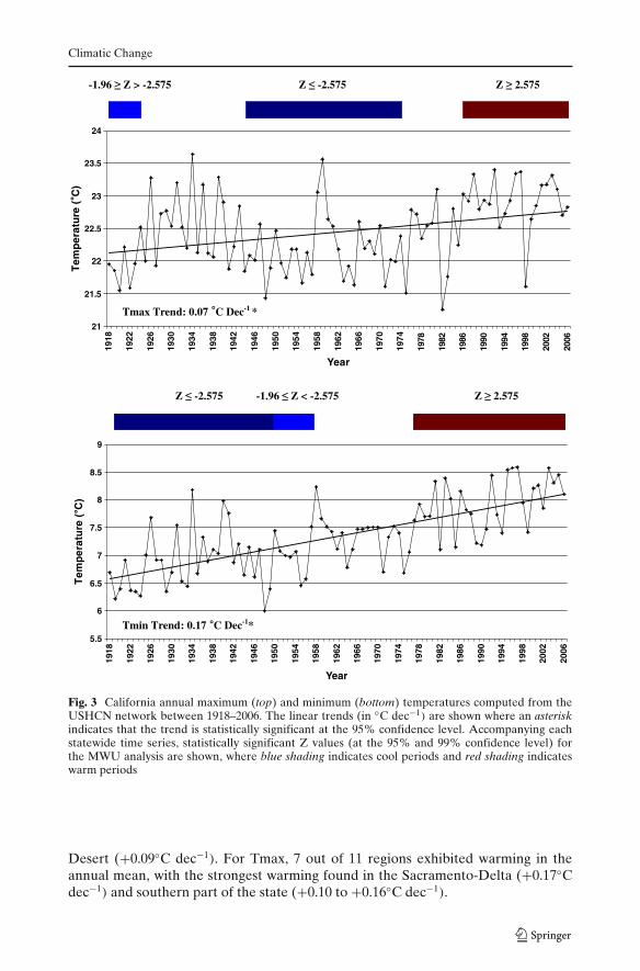
Time series of annual California Tmin and Tmax temperatures from USHCNdata between 1918–2006 are shown in Fig. 3. Annual temperature trends showedstatistically significant warming (95% confidence level) for both Tmin and Tmax, butwith a much larger warming in Tmin (+0.17◦C dec−1) compared to Tmax (+0.07◦Cdec−1). Despite significant differences in long-term trends, annual Tmin and Tmaxwere significantly correlated (r = 0.61), suggesting the influence of common forcingmechanisms.

4 Regional temperature trends using USHCN data

4.1 Annual analysis: 1918–2006

While distinct warming trends were observed for the state, a more detailed in-vestigation was conducted by spatially stratifying the trends. Annual temperaturetrends computed for the 1918–2006 period for each of the 11 defined climateregions using USHCN data are shown in Fig. 4. For Tmin, annual trends for eachregion showed warming (statistically significant at the 95% confidence level), withthe largest warming found in parts of the Central Valley and Southern California(i.e., Sacramento-Delta (+0.26◦C dec−1), South Interior (+0.22◦C dec−1)) and theweakest significant warming found in the Sierras (+0.06◦C dec−1) and the Mojave

Climatic Change

-1.96 Z > -2.575 Z -2.575 Z 2.575

21

21.5

22

22.5

23

23.5

24

1918

1922

1926

1930

1 934

1938

1942

1946

1950

1954

1958

1962

1966

1970

1974

1978

1982

1986

1990

1994

1998

2002

2006

Year

Tem

per

atu

re (˚C

)

Z -2.575 -1.96 Z < -2.575 Z 2.575

5.5

6

6.5

7

7.5

8

8.5

9

1918

1922

1926

1930

1934

1938

1942

1946

1950

1954

1958

1962

1966

1970

1974

1978

1982

1986

1990

1994

1998

2002

2006

Year

Tem

per

atu

re ( ˚

C)

Tmax Trend: 0.07 ˚C Dec-1 *

Tmin Trend: 0.17 ˚C Dec-1*

Fig. 3 California annual maximum (top) and minimum (bottom) temperatures computed from theUSHCN network between 1918–2006. The linear trends (in ◦C dec−1) are shown where an asteriskindicates that the trend is statistically significant at the 95% confidence level. Accompanying eachstatewide time series, statistically significant Z values (at the 95% and 99% confidence level) forthe MWU analysis are shown, where blue shading indicates cool periods and red shading indicateswarm periods

Desert (+0.09◦C dec−1). For Tmax, 7 out of 11 regions exhibited warming in theannual mean, with the strongest warming found in the Sacramento-Delta (+0.17◦Cdec−1) and southern part of the state (+0.10 to +0.16◦C dec−1).

Climatic Change

Fig. 4 Annual temperature trends (◦C dec−1) for the 11 climate regions labeled A-K computedbetween 1918–2006 for Tmax (left) and Tmin (right), where the trends that are statistically significantat the 95% confidence level are indicated with an asterisk

4.2 Comparison of annual trends: 1918–2006 with 1970–2006

It is understood that forcings (i.e., natural and anthropogenic) may interact ina nonlinear fashion, thus affecting temperatures across different time and spatialscales. To evaluate this, we compared annual trends across different regions for twodifferent time periods, 1918–2006 and 1970–2006. The most prominent feature inthis comparison (Fig. 5) was accelerated warming trends from 1970–2006. StatewideTmax trends between 1970–2006 (+0.27◦C dec−1) were more than three times aslarge as the trend between 1918–2006 (+0.07◦C dec−1), while Tmin trends between1970–2006 (+0.31◦C dec−1) were almost twice as large as trends between 1918–2006 (+0.17◦C dec−1). The finding that trends for Tmin were larger than Tmaxfor the entire period, while trends in Tmin were nearly the same as Tmax since1970 is qualitatively similar to results observed for global temperature (Vose et al.2005).

Climatic Change

-0.1

0

0.1

0.2

0.3

0.4

0.5

0.6 C

alifo

rnia

N

orth

ern

CA

Sout

hern

CA

Nor

th C

oast

N

orth

Cen

tral

Nor

thea

st

Sier

ra

Sacr

amen

to-D

elta

C

entr

al C

oast

Sa

n Jo

aqui

n Va

lley

Sout

h C

oast

So

uth

Inte

rior

Moh

ave

Des

ert

Sono

ran

Des

ert

Tren

ds

(C

Dec

-1)

Region

1918-2006 1970-2006

0

0.1

0.2

0.3

0.4

0.5

0.6

Cal

iforn

ia

Nor

ther

n C

A So

uthe

rn C

A N

orth

Coa

st

Nor

th C

entr

al

Nor

thea

st

Sier

ra

Sacr

amen

to-D

elta

C

entr

al C

oast

Sa

n Jo

aqui

n Va

lley

Sout

h C

oast

So

uth

Inte

rior

Moh

ave

Des

ert

Sono

ran

Des

ert

Tren

ds

(C

Dec

-1)

Region

1918-2006 1970-2006

˚˚

a

b

Fig. 5 A comparison of the statewide and regional annual a Tmax and b Tmin trends (◦C dec−1)

for two time periods, 1918–2006 and 1970–2006, where the bars are solid when the computed trendis statistically significant (95% confidence level) and hashed when the trend is not statisticallysignificant

Although statewide trends in temperature for Tmin and Tmax were about thesame since 1970, there were distinct regional differences. In the northern part of thestate (North Coast, North Central, and Northeast regions), the average Tmax trend

Climatic Change

was +0.20◦C dec−1 while the average Tmin trend was +0.27◦C dec−1. In the southernpart of the state (South Interior, Mojave Desert and Sonoran Desert regions),the average Tmax trend was +0.41◦C dec−1 while the average Tmin trend was+0.37◦C dec−1. The difference in warming trends between these northern andsouthern regions was statistically significant and most pronounced in Tmax. Addi-tionally, since 1970, warming Tmin trends were statistically significant in 10 out of11 regions, while warming Tmax trends were statistically significant in only 6 out of11 regions. Regions that did not observe a statistically significant warming of Tmaxincluded both coastal (North Coast, Central Coast, and South Coast) and montane(Northeast and Sierra) regions of the state.

4.3 Mann–Whitney Z analysis of annual temperatures

To further explore the timing and duration of annual temperature change in Cali-fornia, Mann–Whitney U statistics were used to identify significant warm and coolperiods during 1918–2006 for the USHCN stations. Figures 3 and 6 show the resultsof this analysis for both Tmin and Tmax, where significant sequences of low- andhigh-ranked annual temperatures are indicated at 90%, 95%, and 99% confidencelevels by blue or red shaded bars.

In Fig. 3, the original statewide time series and accompanying MWU statisticsare shown together for Tmax and Tmin. For Tmax, cool periods were identifiedaround 1920 and then between the 1940s and the mid-1970s, while a warm periodwas found after 1986. In contrast, for Tmin there were cool periods between the1920s and the 1950s, and a warm period after the mid-1970s. In the case of Tmin, thepatterns of warm and cold years followed a somewhat linear increase in temperaturesas seen in the time series. However Tmax temperatures were quite different, withtwo distinct cold periods accompanied by a warmer recent period. Note that in thecase of Tmax, a number of warm years around 1960 were embedded within a 30-year cool period. Since the MWZ method identifies maximum Z values for periodsbetween 6–30 years, in this case the 30-year cool period was more significant thanthe individual cool periods before or after 1960. This analysis also highlights how theuse of linear least-squares regression is insufficient to capture the highly non-linearchanges observed in temperature, while the MWZ method, which quantifies both thetiming and duration of decadal-scale warm and cold periods, is clearly an improvedmethod of characterizing California temperature variability.

Running MWZ statistics were calculated for each of the USHCN stations forTmax and Tmin and are shown in Fig. 6. For Tmax (Fig. 6a), there appear to be twoperiods when a series of warm calendar years were recorded. The first was during∼1925–1942, when approximately 50% of all stations in California experienceda warm Tmax regime, particularly in the northern part of the state. The secondwarm period was between ∼1985–2006, when approximately 80% of all stationsexperienced a warm Tmax regime. Cool Tmax regimes were generally found between1945–1975, but the start and end years of those regimes differ between the stations.In addition, about 50% of the stations showed cool Tmax periods early in the record(1918–1925). For Tmin (Fig. 6b), over 80% of the stations showed significant coolperiods between 1918–1958, and over 85% of the stations showed warm periodsbetween 1978–2006.

Climatic Change

1920 1930 1940 1950 1960 1970 1980 1990 2000

Z < -2.575 -2.575 < Z < -1.96 -1.96 < Z < -1.645 1.645 < Z < 1.96 1.96 < Z < 2.575 2.575 < Za

Fig. 6 Z values computed using running Mann–Whitney U statistics for annual temperaturesduring 1918–2006 for a Tmax and b Tmin from the USHCN stations. Red colors denote warmingtemperatures while blue colors denote cooling temperatures, with the shading from darkest to lightestindicating statistical significance at the 99%, 95% and 90% confidence level respectively. Each ofthe individual station names is given on the right, while the corresponding regions are indicated onthe left

4.4 Seasonal and regional analysis: 1918–2006 and 1970–2006

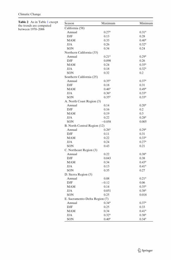
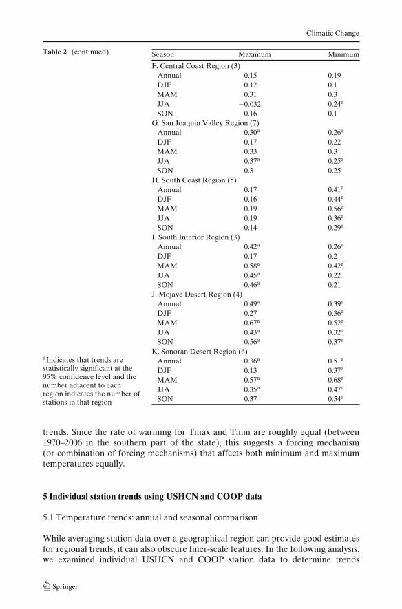
Seasonal trends at the statewide and regional level were analyzed to better under-stand the results from the annual analysis. Tables 1 and 2 provide the statewide andregional Tmax and Tmin trends for each season using the USHCN data for the periodof 1918–2006 and 1970–2006.

Climatic Change

1920 1930 1940 1950 1960 1970 1980 1990 2000

Z < -2.575 -2.575 < Z < -1.96 -1.96 < Z < -1.645 1.645 < Z < 1.961.96 < Z < 2.575 2.575 < Zb

Fig. 6 (continued)

In the period since 1918 (Table 1), the statewide seasonal trends were onlystatistically significant for Tmin and range from +0.14◦C dec−1 (DJF) to +0.21◦Cdec−1 (JJA). In the period since 1970 (Table 2), the statewide seasonal trends werelarger in magnitude, but again only significant for Tmin and during MAM (+0.40◦Cdec−1) and JJA (+0.32◦C dec−1).

At the regional level, Tmax trends were primarily statistically significant in thesouthern part of the state. From 1970–2006 (Table 2), the largest warming in Tmaxoccurred in MAM in the southern part of the state, whereas statistically significantwarming was identified in relatively few regions apart from the southern interiorregions (South Interior, Mojave Desert, and Sonoran Desert) during MAM (+0.61◦Cdec−1), JJA (+0.41◦C dec−1), and SON (+0.46◦C dec−1). For Tmin, the strongest

Climatic Change

Table 1 Annual and seasonalmaximum and minimumtemperatures trends(◦C dec−1) during 1918–2006for California and the 11defined climate regions basedon the USHCN network

Season Maximum Minimum

California (58)Annual 0.071a 0.17a

DJF 0.078 0.14a

MAM 0.088 0.15a

JJA 0.069 0.21a

SON 0.045 0.18a

Northern California (33)Annual 0.05 0.17a

DJF 0.058 0.12a

MAM 0.067 0.15a

JJA 0.053 0.22a

SON 0.024 0.17a

Southern California (25)Annual 0.10a 0.17a

DJF 0.1 0.17a

MAM 0.11a 0.16a

JJA 0.11a 0.17a

SON 0.078a 0.18a

A. North Coast Region (3)Annual 0.085a 0.12a

DJF 0.096a 0.13a

MAM 0.098a 0.15a

JJA 0.11a 0.13a

SON 0.028 0.053B. North Central Region (12)

Annual 0.026 0.17a

DJF 0.045 0.12a

MAM 0.002 0.12a

JJA 0.009 0.20a

SON 0.039 0.17a

C. Northeast Region (3)Annual −0.044 0.20a

DJF 0.091 0.12MAM −0.004 0.18a

JJA −0.081 0.30a

SON −0.19a 0.19a

D. Sierra Region (5)Annual −0.036 0.058a

DJF −0.074 0.002MAM 0.01 0.077JJA 0.062 0.13a

SON −0.097 0.023E. Sacramento-Delta Region (7)

Annual 0.17a 0.26a

DJF 0.14a 0.19a

MAM 0.21a 0.23a

JJA 0.16a 0.32a

SON 0.17a 0.29a

Climatic Change

Table 1 (continued)

aIndicates that trends arestatistically significant at the95% confidence level and thenumber adjacent to eachregion indicates the number ofstations in that region

Season Maximum Minimum

F. Central Coast Region (3)Annual 0.12a 0.15a

DJF 0.12a 0.12a

MAM 0.17a 0.17a

JJA 0.13a 0.20a

SON 0.059 0.10a

G. San Joaquin Valley Region (7)Annual 0.016 0.17a

DJF −0.016 0.12a

MAM 0.065 0.14a

JJA −0.003 0.21a

SON 0.008 0.21a

H. South Coast Region (5)Annual 0.13a 0.18a

DJF 0.16a 0.22a

MAM 0.12a 0.14a

JJA 0.15a 0.19a

SON 0.074a 0.18a

I. South Interior Region (3)Annual 0.16a 0.22a

DJF 0.26a 0.19a

MAM 0.21a 0.20a

JJA 0.057 0.21a

SON 0.092 0.27a

J. Mojave Desert Region (4)Annual 0.13a 0.093a

DJF 0.13a 0.13a

MAM 0.16a 0.12a

JJA 0.095 0.085SON 0.12a 0.012

K. Sonoran Desert Region (6)Annual 0.10a 0.17a

DJF 0.05 0.18a

MAM 0.066 0.17a

JJA 0.18a 0.13a

SON 0.11a 0.22a

warming trends occurred during MAM and were largest in the southern part of thestate. While statewide trends during MAM (+0.40◦C dec−1) were at least 25% largerthan any other season, the largest regional trends were found in the southern interiorregions during MAM (+0.54◦C dec−1), although relatively strong warming (+0.3 to+0.4◦C dec−1) was also apparent during the other seasons in this region. The trendtowards a warmer spring in California has also been noted in other studies (e.g.,Cayan et al. 2008). In contrast, the majority of regional trends during DJF were notsignificant for either Tmin or Tmax trends.

This seasonal analysis offers distinct signatures of the regional climate that mayoffer clues as to the source of these changes. In California, by far the largest warmingbetween 1970–2006 occurred in the southern part of the state (i.e., South Interior,Mojave Desert, and Sonoran Desert regions) during MAM for both Tmin and Tmax

Climatic Change

Table 2 As in Table 1 exceptthe trends are computedbetween 1970–2006

Season Maximum Minimum

California (58)Annual 0.27a 0.31a

DJF 0.13 0.28MAM 0.33 0.40a

JJA 0.26 0.32a

SON 0.34 0.24Northern California (33)

Annual 0.21a 0.29a

DJF 0.098 0.26MAM 0.24 0.35a

JJA 0.18 0.32a

SON 0.32 0.2Southern California (25)

Annual 0.35a 0.37a

DJF 0.18 0.31MAM 0.46a 0.49a

JJA 0.36a 0.33a

SON 0.35a 0.33a

A. North Coast Region (3)Annual 0.14 0.20a

DJF 0.16 0.2MAM 0.19 0.3JJA 0.22 0.28a

SON −0.058 0.005B. North Central Region (12)

Annual 0.26a 0.29a

DJF 0.11 0.31MAM 0.22 0.33a

JJA 0.24 0.27a

SON 0.43 0.21C. Northeast Region (3)

Annual 0.22 0.38a

DJF 0.043 0.38MAM 0.34 0.43a

JJA 0.13 0.41a

SON 0.35 0.27D. Sierra Region (5)

Annual 0.08 0.21a

DJF −0.12 0.06MAM 0.14 0.35a

JJA 0.051 0.38a

SON 0.25 0.018E. Sacramento-Delta Region (7)

Annual 0.34a 0.37a

DJF 0.25 0.33MAM 0.34 0.41a

JJA 0.32a 0.38a

SON 0.40a 0.34a

Climatic Change

Table 2 (continued)

aIndicates that trends arestatistically significant at the95% confidence level and thenumber adjacent to eachregion indicates the number ofstations in that region

Season Maximum Minimum

F. Central Coast Region (3)Annual 0.15 0.19DJF 0.12 0.1MAM 0.31 0.3JJA −0.032 0.24a

SON 0.16 0.1G. San Joaquin Valley Region (7)

Annual 0.30a 0.26a

DJF 0.17 0.22MAM 0.33 0.3JJA 0.37a 0.25a

SON 0.3 0.25H. South Coast Region (5)

Annual 0.17 0.41a

DJF 0.16 0.44a

MAM 0.19 0.56a

JJA 0.19 0.36a

SON 0.14 0.29a

I. South Interior Region (3)Annual 0.42a 0.26a

DJF 0.17 0.2MAM 0.58a 0.42a

JJA 0.45a 0.22SON 0.46a 0.21

J. Mojave Desert Region (4)Annual 0.49a 0.39a

DJF 0.27 0.36a

MAM 0.67a 0.52a

JJA 0.43a 0.32a

SON 0.56a 0.37a

K. Sonoran Desert Region (6)Annual 0.36a 0.51a

DJF 0.13 0.37a

MAM 0.57a 0.68a

JJA 0.35a 0.47a

SON 0.37 0.54a

trends. Since the rate of warming for Tmax and Tmin are roughly equal (between1970–2006 in the southern part of the state), this suggests a forcing mechanism(or combination of forcing mechanisms) that affects both minimum and maximumtemperatures equally.

5 Individual station trends using USHCN and COOP data

5.1 Temperature trends: annual and seasonal comparison

While averaging station data over a geographical region can provide good estimatesfor regional trends, it can also obscure finer-scale features. In the following analysis,we examined individual USHCN and COOP station data to determine trends

Climatic Change

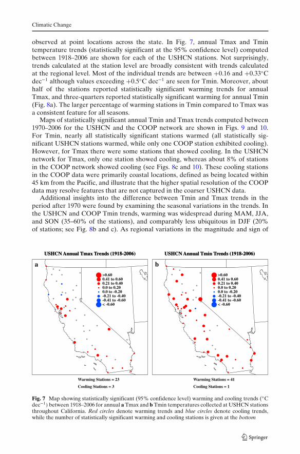
observed at point locations across the state. In Fig. 7, annual Tmax and Tmintemperature trends (statistically significant at the 95% confidence level) computedbetween 1918–2006 are shown for each of the USHCN stations. Not surprisingly,trends calculated at the station level are broadly consistent with trends calculatedat the regional level. Most of the individual trends are between +0.16 and +0.33◦Cdec−1 although values exceeding +0.5◦C dec−1 are seen for Tmin. Moreover, abouthalf of the stations reported statistically significant warming trends for annualTmax, and three-quarters reported statistically significant warming for annual Tmin(Fig. 8a). The larger percentage of warming stations in Tmin compared to Tmax wasa consistent feature for all seasons.

Maps of statistically significant annual Tmin and Tmax trends computed between1970–2006 for the USHCN and the COOP network are shown in Figs. 9 and 10.For Tmin, nearly all statistically significant stations warmed (all statistically sig-nificant USHCN stations warmed, while only one COOP station exhibited cooling).However, for Tmax there were some stations that showed cooling. In the USHCNnetwork for Tmax, only one station showed cooling, whereas about 8% of stationsin the COOP network showed cooling (see Figs. 8c and 10). These cooling stationsin the COOP data were primarily coastal locations, defined as being located within45 km from the Pacific, and illustrate that the higher spatial resolution of the COOPdata may resolve features that are not captured in the coarser USHCN data.

Additional insights into the difference between Tmin and Tmax trends in theperiod after 1970 were found by examining the seasonal variations in the trends. Inthe USHCN and COOP Tmin trends, warming was widespread during MAM, JJA,and SON (35–60% of the stations), and comparably less ubiquitous in DJF (20%of stations; see Fig. 8b and c). As regional variations in the magnitude and sign of

>0.60 0.41 to 0.60 0.21 to 0.40 0.0 to 0.20

USHCN Annual Tmax Trends (1918-2006) USHCN Annual Tmin Trends (1918-2006)

0.0 to -0.20 -0.21 to -0.40 -0.41 to -0.60 < -0.60

Warming Stations = 23

Cooling Stations = 3

>0.60 0.41 to 0.60 0.21 to 0.40 0.0 to 0.20

USHCN Annual Tmax Trends (1918-2006)

a

USHCN Annual Tmin Trends (1918-2006)

b

0.0 to -0.20 -0.21 to -0.40 -0.41 to -0.60 < -0.60

Warming Stations = 41

Cooling Stations = 1

Fig. 7 Map showing statistically significant (95% confidence level) warming and cooling trends (◦Cdec−1) between 1918–2006 for annual a Tmax and b Tmin temperatures collected at USHCN stationsthroughout California. Red circles denote warming trends and blue circles denote cooling trends,while the number of statistically significant warming and cooling stations is given at the bottom

Climatic Change

0

20

40

60

80

100

ANN DJF MAM JJA SON ANN DJF MAM JJA SON

Sta

tio

ns

(%)

Tmax

1918-2006 (USHCN)

Cooling stations

Warming stations

0

20

40

60

80

100

ANN DJF MAM JJA SON ANN DJF MAM JJA SON

Sta

tio

ns

(%)

Tmax

1970-2006 (USHCN)

Cooling stations

Warming stations

0

20

40

60

80

100

ANN DJF MAM JJA SON ANN DJF MAM JJA SON

Sta

tio

ns

(%)

Tmax

1970-2006 (COOP)

Cooling stations

Warming stations

Tmin

Tmin

Tmin

a

b

c

Fig. 8 The percentage of statistically significant (95% confidence level) warming and cooling trendsfor annual and seasonal Tmax and Tmin during the periods of a 1918–2006 for the USHCN data,b 1970–2006 for the USHCN data, and c 1970–2006 for the COOP data

Climatic Change

>0.60 0.41 to 0.60 0.21 to 0.40 0.0 to 0.20 0.0 to -0.20 -0.21 to -0.40 -0.41 to -0.60 < -0.60

Warming Stations = 36

Cooling Stations = 1

>0.60 0.41 to 0.60 0.21 to 0.40 0.0 to 0.20

USHCN Annual Tmax Trends (1970-2006)

a

USHCN Annual Tmin Trends (1970-2006)

b

0.0 to -0.20 -0.21 to -0.40 -0.41 to -0.60 < -0.60

Warming Stations = 40

Cooling Stations = 0

Fig. 9 Map showing statistically significant (95% confidence level) warming and cooling trends (◦Cdec−1) between 1970–2006 for annual a Tmax and b Tmin temperatures collected at USHCN stationsthroughout California. Red circles denote warming trends and blue circles denote cooling trends,while the number of statistically significant warming and cooling stations is given at the bottom

>0.60 0.41 to 0.60 0.21 to 0.40 0.00 to 0.20 0.00 to -0.20 -0.21 to -0.40 -0.41 to -0.60 < -0.60

Warming Stations = 56

Cooling Stations = 15

>0.60 0.41 to 0.60 0.21 to 0.40 0.00 to 0.20

COOP Annual Tmax Trends (1970-2006)

a

COOP Annual Tmin Trends (1970-2006)

b

0.00 to -0.20 -0.21 to -0.40 -0.41 to -0.60 < -0.60

Warming Stations = 94

Cooling Stations = 1

Fig. 10 As in Fig. 9 except that the trends are computed from the COOP network

Climatic Change

Tmin were largely muted, one might be inclined to suggest that the primary forcingmechanism responsible for changes in Tmin are large scale processes includinganthropogenic forcings and large-scale climate variability.

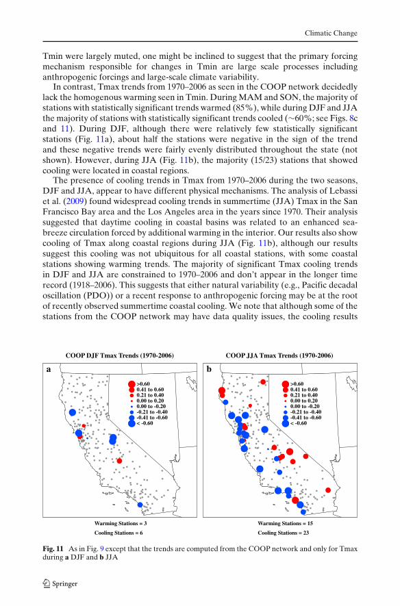
In contrast, Tmax trends from 1970–2006 as seen in the COOP network decidedlylack the homogenous warming seen in Tmin. During MAM and SON, the majority ofstations with statistically significant trends warmed (85%), while during DJF and JJAthe majority of stations with statistically significant trends cooled (∼60%; see Figs. 8cand 11). During DJF, although there were relatively few statistically significantstations (Fig. 11a), about half the stations were negative in the sign of the trendand these negative trends were fairly evenly distributed throughout the state (notshown). However, during JJA (Fig. 11b), the majority (15/23) stations that showedcooling were located in coastal regions.

The presence of cooling trends in Tmax from 1970–2006 during the two seasons,DJF and JJA, appear to have different physical mechanisms. The analysis of Lebassiet al. (2009) found widespread cooling trends in summertime (JJA) Tmax in the SanFrancisco Bay area and the Los Angeles area in the years since 1970. Their analysissuggested that daytime cooling in coastal basins was related to an enhanced sea-breeze circulation forced by additional warming in the interior. Our results also showcooling of Tmax along coastal regions during JJA (Fig. 11b), although our resultssuggest this cooling was not ubiquitous for all coastal stations, with some coastalstations showing warming trends. The majority of significant Tmax cooling trendsin DJF and JJA are constrained to 1970–2006 and don’t appear in the longer timerecord (1918–2006). This suggests that either natural variability (e.g., Pacific decadaloscillation (PDO)) or a recent response to anthropogenic forcing may be at the rootof recently observed summertime coastal cooling. We note that although some of thestations from the COOP network may have data quality issues, the cooling results

Warming Stations = 3

Cooling Stations = 6

>0.60 0.41 to 0.60 0.21 to 0.40 0.00 to 0.20

>0.60 0.41 to 0.60 0.21 to 0.40 0.00 to 0.20

COOP DJF Tmax Trends (1970-2006)

a

COOP JJA Tmax Trends (1970-2006)

b

0.00 to -0.20 -0.21 to -0.40 -0.41 to -0.60 < -0.60

0.00 to -0.20 -0.21 to -0.40 -0.41 to -0.60 < -0.60

Warming Stations = 15

Cooling Stations = 23

Fig. 11 As in Fig. 9 except that the trends are computed from the COOP network and only for Tmaxduring a DJF and b JJA

Climatic Change

appear to be robust and suggest that local-scale changes may be obscured in coarserresolution observational datasets.

5.2 Analysis of COOP trends in DJF since 1970

An approach linking the covariability of temperature and precipitation is presentedto provide insight into the overall neutral or weak warming trends found in Tmaxtrends over the state from 1970–2006. The overall lack of warming noted in DJFTmax from across the state of California appears as an anomaly to the widespreadwarming observed across other seasons and for Tmin. A majority of stations acrossthe state exhibited a significant negative correlation between DJF Tmax and DJFaccumulated precipitation (Fig. 12a). The correlation between precipitation andtemperature trends was also discussed, although not extensively quantified by Cayanet al. (2008). The geographic representation of the temperature–precipitation covari-ability was strong (r < −0.5) across the Sierra Nevada, coast range, and interiorportions of Southern California, suggesting that Tmax is suppressed during wetwinters, and vice versa. In general, the synoptic-scale patterns that bring wintertimeprecipitation are associated with dynamical (cooler air mass) and thermodynamical(increased cloud cover, snow cover, and soil moisture) mechanisms that suppressTmax. The only widespread regions void of the anticorrelation in temperature–precipitation records exist across the central and southern Central Valley. Extensiveradiation fog often inundates the Central Valley during dry mid-winter blockingpatterns, therein suppressing Tmax across the low-lying valley. By contrast, sig-nificant positive correlations between DJF Tmin and precipitation were observed fora majority of stations statewide from 1970–2006, suggesting that Tmin is suppressedduring dry winters, and vice versa (Fig. 12b). The strong covariability betweenTmin and precipitation is argued to arise through thermodynamic mechanisms (e.g.,radiative cooling) associated with precipitation (e.g., cloud cover).

>0.60 0.41 to 0.60 0.21 to 0.40 0.00 to 0.20 0.00 to -0.20 -0.21 to -0.40 -0.41 to -0.60 < -0.60

a

>0.60 0.41 to 0.60 0.21 to 0.40 0.00 to 0.20 0.00 to -0.20 -0.21 to -0.40 -0.41 to -0.60 < -0.60

b

Fig. 12 Statistically significant correlation coefficients for accumulated precipitation and a winter(DJF) maximum temperature and b winter (DJF) minimum temperature over the period 1970–2006for COOP stations within California

Climatic Change

Over the 1970–2006 period, the state of California observed an increase inwinter precipitation with 98% of stations showing positive, albeit, generally non-significant trends (10% of stations, most located in the northern portion of the state,showed statistically significant positive trends in precipitation). It is hypothesizedthat increases in precipitation over the last 35 years, and moreover the consortiumof synoptic conditions associated with these increases, have acted to modulateregional trends for Tmax and Tmin. To account for the influence of precipitationon winter temperature trends across the state we remove the collinear influence ofprecipitation on temperature using Eq. 1,

Ti,R (t) = Ti (t) − αi P′i (t) , (1)

where Ti,R(t) represents the residual temperature of a given station, i,; at time t,the regression coefficient of temperature to precipitation is αi, and the seasonalprecipitation anomaly is P′

i(t). Winter Tmax and Tmin trends are calculated for boththe observed time series and the residual time series so that the influence of trendsin precipitation can be evaluated.

Observed trends in DJF Tmax for 1970–2006 were relatively weak across the statewith a statewide trend of +0.07◦C dec−1 with only a few stations showing a significantpositive trend. Linear trends of the residual temperature, after removing the linearcontribution from winter precipitation, exhibited over twice as many stations (12%)with statistically significant warming, and a statewide trend of +0.12◦C dec−1. Bycontrast, observed trends in DJF Tmin for COOP stations for 1970–2006 exhibited astatewide trend of +0.35◦C dec−1 with over a third of all stations showing significantwarming trends. Upon removal of the collinear influence of precipitation, thestatewide trend was +0.22◦C dec−1. It is presently unclear whether the increasesin DJF precipitation observed during this period are consistent with anthropogenicclimate change or natural variability; however, it is clear that the lack of widespreadwarming in Tmax, and high rate of warming in Tmin can be partially accounted forby increases in precipitation.

6 Discussion of forcing mechanisms

This analysis offers two important diagnostics that may be useful in characterizingstatewide changes in temperature during 1918–2006. One is the striking consistencyin widespread shifts of temperature that appear throughout the state, and theother is the notable difference between Tmin and Tmax temperature variations.For example, the remarkably consistent end of cool Tmin periods in 1958 and thesimilarly common beginning of warm periods around 1978 suggest a universal changein California-wide climate patterns on Tmin that are not uniformly reflected in Tmax.The disparity between temperature signals from Tmin and Tmax suggests distinctlyseparate forcing mechanisms that operate at different spatial scales. Alfaro et al.(2006) showed that summertime variations in Tmin over the central and western U.S.are controlled more by larger-scale forcings (e.g., sea surface temperatures), whileTmax is controlled more by local-scale forcings (e.g., soil moisture and cloudiness).

The patterns of temperature change for Tmin and Tmax provide clues aboutthe role of different forcing mechanisms on California’s climate. Both natural and

Climatic Change

anthropogenic forcing mechanisms have been shown to influence global and regionalclimate (e.g., IPCC 2007). Climate attribution studies have examined the influenceof anthropogenic forcing (e.g., Bonfils et al. 2008) and internal climate variability(e.g., Hoerling et al. 2010) on regional climate. Although it is increasingly difficult toattribute changes at local scales due to weak signal-to-noise ratios (e.g., Hegerl et al.2007), several forcing mechanisms are hypothesized to have influenced temperaturesin California. Increased concentrations of GHGs are hypothesized to directly (i.e.,via radiative forcing) increase Tmax and Tmin at similar rates over large spatialscales (i.e., Zhou et al. 2009). Increased anthropogenic aerosols are hypothesizedto decrease Tmax and have a stronger regional signal that may vary over time.Indirect mechanisms associated with these anthropogenic-forcing mechanisms mayresult in more complex regional signatures. For example, changes in clouds, asa consequence of modified aerosol concentration, atmospheric water vapor, soilmoisture, or changes in ocean–atmosphere circulation would also be expected todifferentially influence Tmax and Tmin. California’s land surface has also changedprofoundly over the last century, with urbanization and large-scale irrigation amongthe largest changes observed. Urbanization appears to raise primarily Tmin (e.g.,LaDochy et al. 2007), while irrigation appears to both cool maximum temperaturesand warm minimum temperatures (e.g., Bonfils and Lobell 2007; Kueppers et al.2007). Finally, superimposed on these external forcings is natural internal variabilitymanifested through large-scale coupled atmosphere–ocean phenomena, such as ElNino-Southern Oscillation and the PDO, that have a noted influence on temperatureand precipitation across California (e.g., Redmond and Koch 1991; LaDochy et al.2007). Changes in atmospheric circulation regimes over the latter half of the twenti-eth century have been shown to influence regional temperatures (e.g., Wu and Straus2004; Abatzoglou and Redmond 2007; Abatzoglou 2010) and are hypothesized tohave influenced the observed evolution of Tmax and Tmin across California.

In the above MWZ analysis, the patterns of annual temperature change for Tmin(Fig. 6b) indicate steady widespread warming (cool periods to warm periods) overthe 80-year period, suggesting large-scale forcing such as increases in GHGs. Thispattern is similar for different seasons except MAM (not shown), where a statewidecool period is found between the 1940s and 1970s. While this corresponds to the well-documented cold period of the PDO (Mantua et al. 1997), it is presently unclear whyspring minimum temperatures would be affected more than other seasons if the PDOis responsible for these changes.

For Tmax, the patterns identified by the MWZ method (Fig. 6a) vary more inspace and time compared to Tmin. The most pronounced pattern in the annualvariations is warm-cold-warm, where a warm period early in the century is followedby a cool period mid century and then another warm period towards the end ofthe record. While the MWZ analysis for each season (not shown) generally followsthis pattern, there are some distinct variations. For example, during MAM a veryconsistent statewide cooling period (in 80% of the stations) was found betweenthe late 1940s and the mid 1960s. Because this pattern is so consistent throughoutthe state, it is suggested that variability associated with large-scale circulation isresponsible, rather than a more localized signature associated with land-use changeor aerosols. However, during JJA, over 70% of the stations from irrigated areas (i.e.,North Central Region, Sacramento-Delta Region, and San Joaquin Valley Region)showed cooling periods between 1920 and 1980, and warming since 1990 or 2000.

Climatic Change

In this case, one would suspect that irrigation, which grew in California from theearly century to around the 1980s, is a likely contributor to these changes. Whilethis analysis cannot directly attribute any of these forcings to observed evolution ofregional temperature trends, we present this analysis to provide guidance for laterclimate attribution studies.

7 Summary and conclusions

California temperatures have seen significant changes over the last 80 years, withvariations both in time and in space and differential changes in Tmin and Tmax. Ingeneral, the southern part of the state, and the southern deserts in particular, hasexperienced the greatest amount of warming, and this warming has accelerated overthe last 35 years. The greater warming in Southern California compared to NorthernCalifornia and the recent amplification in warming has been more pronouncedin Tmax compared to Tmin. Although Tmin also show significant warming, thiswarming is more uniformly distributed throughout the state. Since 1970, the largestwarming is found during MAM, both for Tmin and Tmax. The similar rates ofwarming for Tmin and Tmax in Southern California are distinct from the larger Tminwarming in Northern California. In general, DJF shows the weakest warming forboth Tmin and Tmax throughout the state.

Mann–Whitney Z analyses conducted on annual USHCN station data identifybroad-scale consecutive warm and cold years throughout the 88-year record anddistinct patterns for Tmin and Tmax. For Tmin, colder years are prevalent between1920 and 1958, while warmer years are observed after 1978. The pattern in Tmax isquite different, with warmer years found between 1925 and 1942 and again starting inthe period 1985 to 1995, while cooler years are observed between 1945 and 1975. Theremarkable statewide shift in warming and cooling years for Tmin suggests large-scale forcing, a distinctly different pattern from the warming and cooling seen inTmax, which suggests more local-scale forcing. The MWZ method is shown to be abetter analysis tool for analyzing multi-decadal variability compared to linear trends.

Further differences between Tmin and Tmax are found by examining seasonaltrends in the individual COOP data since 1970. Although large-scale warming isfound for Tmin trends during all seasons, during DJF and JJA we find that abouthalf the significant Tmax trends are cooling. During DJF, the lack of warming forTmax throughout California is found only since 1970, and it is suggested that anincrease in precipitation (and thus cloudiness) over California in the last 35 years hasmasked warming. By contrast, increases in winter precipitation since 1970 are alsoshown to have accelerated the rate of warming of Tmin, therein providing insight intocontrasting mechanisms behind regional Tmax and Tmin trends. Patterns of coolingduring JJA are largely constrained to coastal areas, which suggest a relationship withocean temperatures.

A variety of forcing mechanisms appear to have influenced climate in Californiaover different space and time scales. Foremost are the increases in well-mixedgreenhouse gases that have been carefully documented and attributed to most of theglobal- and continental-scale warming observed since 1970. However, other changessuch as land-use changes, variations in precipitation, regional-to-local feedbackprocesses, and changes in ocean temperatures and sea breeze are also likely to have

Climatic Change

played a role in the spatial and temporal character of California temperatures overthe past century. The aim of our study has been to characterize the changes inCalifornia’s climate so that future attribution studies can be performed to betterunderstand the interrelationships between the various forcing mechanisms. Wesuggest that the Mann–Whitney Z analysis, coupled with output from downscaledand regional climate models, would be an excellent tool for such attribution studies,especially where identifying the role of local- versus large-scale forcing is important.This work has already begun with the ultimate aim of improving our projections offuture changes in California’s climate.

Acknowledgements We thank Bereket Lebassi for help in acquiring the NWS COOP dataset andProfessor Bob Bornstein for many helpful discussions. This work was supported by NSF’s FacultyEarly Career Development (CAREER) Program, Grant ATM-0449996.

References

Abatzoglou JT (2010) Influence of the PNA on declining mountain snowpack in the Western UnitedStates. Int J Climatol. doi:10.1002/joc.2137

Abatzoglou JT, Redmond KT (2007) The asymmetry of trends in spring and autumn tempera-ture and circulation regimes over western North America. Geophys Res Lett 34. doi:10.1029/2007GL030891

Abatzoglou JT, Redmond KT, Edwards LE (2009) Classification of regional climate variability inthe State of California. Appl Meteorol Climatol 48:1527–1541

Alfaro EJ, Gershunov A, Cayan D (2006) Prediction of summer maximum and minimum temper-ature over the Central and Western United States: the roles of soil moisture and sea surfacetemperature. J Clim 19:1407–1421

Bonan GB (2001) Observational evidence for reduction of daily maximum temperature by croplandsin the midwest United States. J Clim 14:2430–2442

Bonfils C, Lobell DB (2007) Empirical evidence for a recent slowdown in irrigation-induced cooling.Proc Natl Acad Sci 104:13582–13587

Bonfils C, Duffy PB, Lobell DB (2006) Comments on methodology and results of calculating cen-tral California surface temperature trends: evidence of human-induced climate change? J Clim20:4486–4489

Bonfils C, Duffy PB, Santer BD, Wigley TML, Lobell DB, Phillips TJ, Doutriaux C (2008) Iden-tification of external influences on temperatures in California. Climatic Change 87(suppl 1):S43–S55. doi:10.1007/s10584-007-9374-9

Cayan DR, Maurer EP, Dettinger MD, Tyree M, Hayhoe K (2008) Climate change scenarios for theCalifornia region. Climatic Change 87(suppl 1):S21–S42. doi:10.1007/s10584-007-9377-6

Christy JR, Norris WB, Redmond KT, Gallo KP (2006) Methodology and results of calculatingcentral California surface temperature trends: evidence of human-induced climate change? JClim 19:548–563

Cordero E, Forster PMdF (2006) Stratospheric variability and trends in models used for the IPCCAR4. Atmos Chem Phys 6:5369–5380

Hayhoe K, Cayan D, Field CB, Frumhoff PC, Maurer EP, Miller NL, Moser SC, Schneider SH,Cahill KN, Cleland EE, Dale L, Drapek R, Hanemann RM, Kalkstein LS, Lenihan J, Lunch CK,Neilson RP, Sheridan SC, Verville JH (2004) Emissions pathways, climate change, and impactson California. Proc Natl Acad Sci 101:12422–12427

Hegerl GC, Zwiers FW, Braconnot P, Gillett NP, Luo Y, Marengo J, Nicholls N, Penner JE, StottPA (2007) Understanding and attributing climate change. Chapter 9 in Climate change 2007:the physical science basis. Contribution of Working Group 1 to the Fourth Assessment Reporton the Intergovernmental Panel on Climate Change. Cambridge University Press, Cambridge,pp 663–745

Hoerling M, Eischeid J, Perlwitz J (2010) Regional precipitation trends: distinguishing natural vari-ability from anthropogenic forcing. J Clim 23:2131–2145

Climatic Change

IPCC (2007) Climate change 2007: the physical science basis. Contribution of Working Group 1 tothe Fourth Assessment Report on the Intergovernmental Panel on Climate Change. CambridgeUniversity Press, Cambridge

Kalnay E, Cai M (2003) Impact of urbanization and land-use change on climate. Nature 423:528–531Kueppers LM, Snyder MA, Sloan LC (2007) Irrigation cooling effect: regional climate forcing by

land-use change. Geophys Res Lett 34:L03703. doi:10 1029/2006GL028679LaDochy S, Medina R, Patzert W (2007) Recent California climate variability: spatial and temporal

patterns in temperature trends. Clim Res 33:159–169Lebassi B, Gonzalez J, Fabris D, Maurer E, Miller N, Milesi C, Switzer P, Bornstein R (2009)

Observed 1970–2005 cooling of summer daytime temperatures in coastal California. J Clim22:3558–3573

Lund R, Seymour L, Kafadar K (2001) Temperature trends in the United States. Environmetrics12:673–690. doi:610.1002/env.1468

Mantua NJ, Hare SR, Zhang Y, Wallace JM, Francis RC (1997) A Pacific interdecadal climateoscillation with impacts on salmon production. Bull Am Meteorol Soc 78:1069–1079

Mauget SA (2003a) Intra- to multi-decadal climate variability over the Continental United States:1932–1999. J Clim 16:2215–2231

Mauget SA (2003b) Multi-decadal regime shifts in U.S. streamflow, precipitation, and temperatureat the end of the Twentieth Century. J Clim 16:3905–3916

Mendenhall W, Wackerly DD, Sheaffer RL (1990) Mathematical statistics with applications. PWS-Kent, Boston

Peterson TC (2003) Assessment of urban versus rural in situ surface temperature in the contiguousUnited States: no difference found. J Clim 16:2941–2959

Redmond KT, Koch RW (1991) Surface climate streamflow variability in the western UnitedStates and their relationship to large-scale circulation indices. Water Resour Res 27:2381–2399.doi:10.1029/91WR00690

Santer BD, Wigley TML, Boyle JS, Gaffen DJ, Hnilo JJ, Nychka D, Parker DE, Taylor KE (2000)Statistical significance of trends and trend differences in layer-average atmospheric temperaturetime series. J Geophys Res Atmos 105(D6):7337–7356

Saxena VK, Yu S (1998) Searching for a regional fingerprint of aerosol radiative forcing in thesoutheastern US. Geophys Res Lett 25:2833–2836

Stafford JM, Wendler G, Curtis J (2000) Temperature and precipitation of Alaska: 50 year trendanalysis. Theor Appl Climatol 67:33–44

Vose RS, Easterling DR, Gleason B (2005) Maximum and minimum temperature trend for the globe:an update through 2004. Geophys Res Lett 32:L23822. doi:23810.21029/22005GL024379

Wild M, Ohmura A, Makowski K (2007) Impact of global dimming and brightening on globalwarming. Geophys Res Lett 34. doi:10.1029/2006GL028031

Wilks DS (1995) Statistical methods in the atmospheric sciences. Academic Press, San DiegoWilliams CN, Menne MJ, Vose R, Eastering DR (2007) United States Historical Climatology Net-

work monthly temperature and precipitation data. Oak Ridge National Laboratory, Oak Ridge,Tennessee: ORNL/CDIAC-187

Wu QG, Straus DM (2004) On the existence of hemisphere-wide climate variations. J Geophys ResAtmos 109:D06118. doi:10.1029/2003JD004230

Yang F, Kumar A, Wang W, Juang H-MH, Kanamitsu M (2001) Snow-albedo feedback and seasonalclimate variability over North America. J Clim 14:4245–4248

Zhou LM, Dickinson RE, Dirmeyer P, Dai A, Min S-K (2009) Spatiotemporal patterns of changes inmaximum and minimum temperatures in multi-model simulations. Geophys Res Lett 36:L02702.doi:10.1029/2008GL036141