HAL Id: halshs-01238494https://halshs.archives-ouvertes.fr/halshs-01238494

Submitted on 5 Dec 2015

HAL is a multi-disciplinary open accessarchive for the deposit and dissemination of sci-entific research documents, whether they are pub-lished or not. The documents may come fromteaching and research institutions in France orabroad, or from public or private research centers.

L’archive ouverte pluridisciplinaire HAL, estdestinée au dépôt et à la diffusion de documentsscientifiques de niveau recherche, publiés ou non,émanant des établissements d’enseignement et derecherche français ou étrangers, des laboratoirespublics ou privés.

The German unemployment since the Hartz reforms:Permanent or transitory fall?

Gaëtan Stephan, Julien Lecumberry

To cite this version:Gaëtan Stephan, Julien Lecumberry. The German unemployment since the Hartz reforms: Permanentor transitory fall?. Economics Letters, Elsevier, 2015, 136, pp.49-54. �10.1016/j.econlet.2015.08.003�.�halshs-01238494�

The German Unemployment since the Hartz

Reforms: Permanent or Transitory Fall?

Gaëtan Stephan1, Julien Lecumberry

University of Rennes 1 - CREM

June 2015

Abstract

The Hartz reforms were designed to make the German labor market more flexible in order to reverse

the increasing trend of unemployment. This paper employs unobserved components models in order to

distinguish permanent from transitory movements in the German unemployment rate. Our results

show that the permanent component of the German unemployment was reduced in the range of 1.1

and 2.6 percentage points after the Hartz reforms.

J.E.L: C32, E32

Keywords: business cycle, unobserved components, Hartz reforms

1 _University of Rennes 1, France, 7, Place Hoche - CS 86514 35065 Rennes Cedex, Tel: +33(0)2 23 23 33

24, Email adress: gaetanstephan@hotmail.fr

*Title Page

1 Introduction

After having peaked at 11.4 % in 2005, the German unemployment rate recorded a sharp trend reversal

and declined steadily until reaching 5.5 % at the end of 2013. This labor market performance has

received considerable attention, especially during the Great Recession where unemployment slightly

increased (Burda and Hunt (2011)). One popular reason among economists is to give credit to the wide-

ranging Hartz reforms implemented in 2003-2005. The reforms aimed to reverse the increasing trend of

unemployment, particularly by getting long-term unemployed back to work. The four laws Hartz I-IV

consist of a set of measures such as lowering benefits during unemployment, restructuring the federal

labor agency or reducing the social security contributions on labor. Krebs and Scheffel (2013) show that

Hartz reforms led to a substantial reduction in the trend component of unemployment. This paper

attempts to know how much of this fall can be attributed to the trend component.

Unobserved components models allow to distinguish permanent (trend) from transitory (cyclical)

movements in macroeconomic fluctuations. Traditional unobserved components models, employed by

Clark (1987, 1989) or Harvey (1989), set to zero correlation between shocks to the trend and the cycle.

Nevertheless, Morley et al (2003) (MNZ) show that the correlation could be identified and free

estimated by specifying transitory component as an AR (2) process. Sinclair (2009) extends MNZ

method to a multivariate analysis with real GDP and unemployment rate. This methodology suggests a

substantial role for permanent movements unlike traditional models which imply a larger role for

transitory movements. We estimate unobserved components models consisting of unemployment and

real GDP following both Sinclair (2009) and a more conservative approach similar to Clark (1989).

Moreover, Perron and Wada (2009) show that permanent movements become secondary in explaining

overall fluctuations when allowing a structural break in the trend component. Therefore, our models

include structural breaks in the trend component of unemployment and real GDP.

This paper assesses how much the reduction of the German unemployment rate can be attributed to a

permanent component. To anticipate our findings, the permanent component of unemployment was

reduced in the range of 1.1 and 2.6 percentage points after the implementation of the Hartz reforms,

even in the most conservative estimate. Furthermore, the Great Recession accounts for a permanent loss

on the German real GDP. The rest of the paper proceeds as follows. Section 2 describes unobserved

components models employed in our empirical analysis. Section 3 presents and discusses the results

while Section 4 concludes.

2 Model and data

In order to distinguish trend component from cycle component, we resort to a bivariate unobserved

components representation. Building on Clark (1989) and Sinclair (2009), the model consists of

unemployment rate and real GDP. Unemployment rate ! is disentangled into permanent "#! and

transitory components $#!: %& ='(%& + )%&'''*,)

Berger (2011) argues that trend component of unemployment cannot be specified as a simple random

walk for European countries. Following Berger, we represent the trend component of unemployment as

a random walk with drift:

(%& = -%& + (%&., + /%& (2)

0#! = 01# + 2*3 > 4#56 (3)

*Manuscript

Click here to view linked References

where 7#!'is the innovation of permanent component of unemployment. Berger finds for Euro area

unemployment one break occurred in 1985Q1. Before the break, the drift term is estimated to be 0.125

implying an upward trend in unemployment over the first period. After the break, the drift is estimated

to be close to zero. Thus, the permanent component of Euro area unemployment collapses to a simple

random walk. In equation (3), drift equals 01# before the break date labelled by 4# and 01# + 6'*08#5 after. Based on univariate break tests

1, we find one break in 1983Q2. Real GDP 9! is also the sum of

permanent ":! and transitory components $:!: 9! ='":! + $:! (4)

Permanent component of real GDP is specified as a random walk with drift2, where 09! is the average

growth rate of real GDP and 79! represents the innovation as:

":! = 0:! + ":!.1 + 7:! (5)

0:! = 01: + 2;3 > 4:<6 (6)

Following Perron and Wada (2009), equation (5) accounts for one structural break in the drift term. This

specification aims to capture potential shift in the trend component of output. Average growth rate

equals 01: before the break denoted''4:, 01: + 6'*08:5 after. Univariate break tests find a shift in

1991Q1 corresponding to the German reunification. Transitory component of unemployment and real

GDP are modeled as an AR (2) process:

$#! = ?1#$#!.1 +?8#$#!.8 + @#! (7)

$:! = ?1:$:!.1 + ?8:$:!.8 + @:! (8)

The shocks (7:! A 7#!A @:! A @#!) are assumed to be normally distributed with mean zero. The variance-

covariance matrix allows no restrictions on the correlations between any of the contemporaneous

shocks. The variance-covariance matrix is:

BCCDEFG8 E797 E79@9 E79@ E797 EFH8 E7 @9 E7 @ E79@9 E7 @9 EIG8 E@9@ E79@ E7 @ E@9@ EIH8 J

KKL

We confront this correlated unobserved components model to a more conservative approach which

impose restrictions on the variance-covariance matrix, similar to Clark (1989) :

BCDEFG8 M M MM EFH8 M MM M EIG8 E@9@ M M E@ @9 EIH8 J

KL

1 We use tests proposed by Bai and Perron (1998, 2003) and Andrews and Ploberger (1994).

2 The Augmented Dickey-Fuller test with GLS detrending (ADF-GLS) cannot reject the null hypothesis of unit

root for real GDP.

These restrictions assume that the off-diagonal elements of the matrix are set to zero. Okun (1962)

shows that real GDP and unemployment are negatively related through their transitory movements.

Thus, we only allow EIGIH to be free estimated as transitory component of real GDP and unemployment

are linked via Okun's law.

Equations (1)-(8) are cast into state-space form. The parameters of the model are estimated by using the

Kalman Filter algorithm and maximum likelihood estimation.

Quarterly data are extracted from OECD.Stat and covering the period from 1970Q1 until 2013Q4.

Unemployment corresponds with unemployment rate. Real GDP is defined in millions of dollars,

volumes estimates, OECD reference year, annual levels and seasonally adjusted. Real GDP is expressed

in logarithm and multiplied by 100.

3 Results

3.1 Parameters and components estimates

Table 1 reports the maximum likelihood estimates of our different specifications. The first column

presents estimates of Model (1) which allows no restrictions on the variance-covariance matrix. Model

(2) includes structural breaks3 in the drift term of unemployment rate and real GDP. A likelihood ratio

test with a p-value of 0.002 rejects the null hypothesis of no structural breaks. Finally, Model (3) is a

restricted model with zero-covariances between permanent and transitory shocks including structural

breaks.

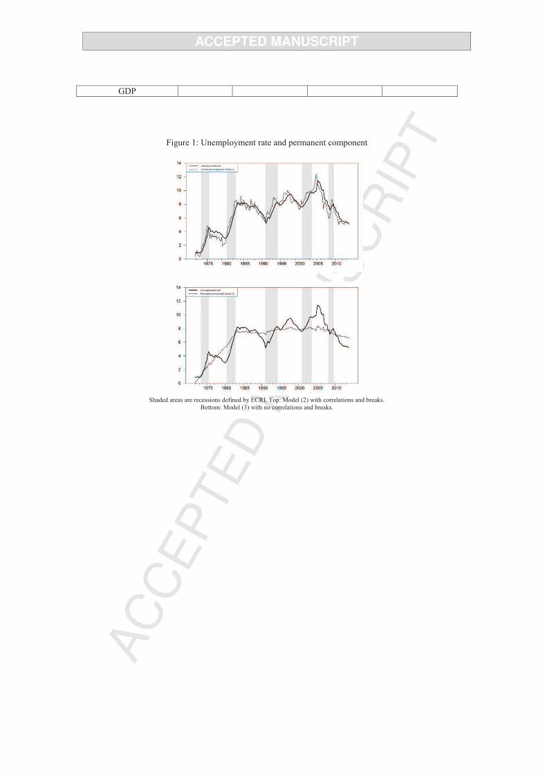
Figure 1 shows the estimated permanent component of unemployment rate based on Model (2).

Movements in the unemployment rate appear to arise mainly from permanent shocks as the estimated

permanent component is quite volatile. In particular, the standard deviation of the permanent innovation

(0.566) is higher than the standard deviation of the first difference of the series (0.281) and slightly

larger than the transitory innovation (0.547). The permanent and transitory innovations show negative

correlation OFHIH with an estimate of -0.958. Allowing correlations between shocks to the trend and the

cycle conduct to a significant part of permanent movements in the unemployment fluctuations.

The drift term 01# is found to be 0.158 % for Model (2) and 0.165 % for Model (3) on the pre-1983

sample. After the structural break, the drift term is estimated to be close to zero and not significant. We

assume that this parameter is subject to one structural change rather than modeling the drift term as a

random walk, implying that the permanent component of unemployment is I(1).

According to the bottom of Figure 1, Model (3) suggests that the increase of the German unemployment

is explained by the permanent component until 1983. After the break, most of the movements arise

mainly from transitory shocks although a decrease in the permanent component is observed since the

mid-2000. Especially, the standard deviation of the transitory innovation (0.159) is larger than the

standard deviation of the permanent innovation (0.148). Without surprise, the persistence of the

transitory unemployment, as measured by the sum of the autoregressive parameters ?1# and'?8#,

presents a high value relative to Model (2).

By multiplying the drift term 0: of real GDP by four, it can be interpreted as the average annual growth

rate of the permanent component. Based on Model (2), the drift term is estimated to be 0.655 before

3 Including structural breaks reduce the size of the permanent and transitory innovations for both unemployment

rate and real GDP.

1991Q1 and 0.354 thereafter. Thus, the permanent component of real GDP has annually grown by 2.6 %

on average before the structural break and 1.4 % after. These estimates are quite similar in Model (3).

Both models agree on a fall of almost 50 % of average annual growth rate after the process of

reunification.

Similar to unemployment, movements in the German real GDP are mainly driven by permanent shocks

in Model (2). The permanent component of real GDP is highly variable as shown by Figure 2 and very

close to the series itself. The standard deviation of the permanent innovation (1.213) is larger than the

standard deviation of the transitory innovation (0.395) and the standard deviation of the first difference

of the series (0.993). These findings suggest a minor role for transitory shocks. Conversely to common

detrending methods, such as bandpass or Hodrick-Prescott filters, Model (2) cannot remove low

frequency movements in real GDP series. Therefore, the transitory component of real GDP, presented in

the Figure 3, looks like small in amplitude and noisy. In addition, the transitory component of real GDP

appears to match poorly recessions4.

Another interesting fact is the variability of the permanent component of the German real GDP during

recessions. The permanent component falls in accord with ECRI recessions, while the transitory

component takes some positive values. Obviously, these facts cast serious doubts about the ability of

Model (2) to generate business cycle. Both Models (1) and (2) found that the correlation OFGIG between

the permanent and transitory components of real GDP is strongly negative: -0.823 in Model (2). This

pattern is consistent with other studies that have examined correlation between trend and cycle using

correlated unobserved components models [Morley et al (2003), Morley (2007), Sinclair (2009), Mitra

and Sinclair (2012)].

Third column of Table 1 presents estimated parameters of Model (3). The results are striking: the

parameters of the restricted model deviate strongly from Models (1) and (2). Fluctuations in real GDP

are primarily due to transitory movements. The standard deviation of the permanent innovation (0.670)

decreases of almost 50 % relative to Model (2) and becomes lower than the standard deviation of the

first difference of real GDP. Consequently, the permanent component of real GDP acts more like a

smooth trend. The transitory component, measured by the sum of the autoregressive parameters,

becomes more persistent: 0.925 versus 0.623 in Model (2). Moreover, the declines in the transitory

component match reasonably well with ECRI recessions, as shown by Figure 3. The restricted

unobserved components approach implies a large and persistent cycle in agreement with business cycle.

3.2 Unemployment downward trend in Hartz reforms

Figure 4 shows the estimated permanent component of unemployment rate based on Model (2) and

Model (3). The picture is limited to 1999 to investigate trend unemployment movements during

implementation of the Hartz reforms and the Great Recession. From 2001 to 2005, the German

unemployment rate rose from 7.8 % to 11.1 % and fall to 8.7 % in 2007 before the onset of the Great

Recession. A striking feature is the slight increase of unemployment during the Great Recession and its

ongoing decrease after the crisis. It is noteworthy to highlight that both models agree on a decrease of

the permanent component of unemployment. We assess the fall in the permanent component from 2007

to 2013 as it corresponds to the onset of the Great Recession5 and the end of the 2005-2007 recovery

6.

According to Model (3), the permanent unemployment was reduced by 1.1 percentage points ranging

from 7.8 % in 2007 to 6.7 % in 2013. Considering Model (2), the permanent unemployment fell from

almost 2.6 percentage points between 2007 and 2013. In addition, the Great Recession appears to have

not any adverse effect on the permanent component on both Models although the unrestricted estimate

provides some volatility during the Great Recession. The decrease of the trend components could be

4 Recessions are defined by the Economic Cycle Research Institute (ECRI).

5 Another reason for this choice is to compare the competing effects of Great Recession and labor market reforms

on unemployment trend. 6 Conversely to 2005, permanent components and actual series are close in 2007.

easily attributed to lagged effects of the Hartz reforms. Although Models (2) and (3) differ strongly

about the importance of permanent and transitory shocks, both models point out a steady fall in the

permanent component of unemployment, even in the most conservative estimate, in the aftermath of the

Hartz reforms7.

Figure 5 presents the permanent component of the German real GDP based on Model (2) and Model (3)

between 1999 and 2013. During the Great Recession, Germany suffered a real GDP decline of almost

6.7 %, the most severe recession in the post-war era. Model (3) suggests that real GDP experienced a

permanent loss of 4.1 %, we conclude that the major part of the recession was captured by the

permanent component. Both Models point out a fall in the permanent component of real GDP during the

Great Recession conversely to the 2001-2003 recession.

4 Conclusion

In this paper, we focus on identifying the importance of permanent versus transitory movements in the

German unemployment since the implementation of the Hartz reforms. The reforms aimed to make the

German labor market more flexible in order to reverse the increasing trend of unemployment. Using

quarterly data from 1970 to 2013, we estimate unobserved components models consisting of

unemployment and real GDP. Considering different specifications, our results show that unemployment

trend was reduced in the range of 1.1 and 2.6 percentage points since the implementation of the Hartz

reforms, although the importance of permanent shocks depends on the estimates. In addition, the results

suggest that Great Recession accounts for a permanent loss on the German real GDP.

7 We would like to thank our anonymous referee for suggesting this comment.

References

Andrews, D. W. K. and Ploberger, W. (1994). Optimal Tests When a Nuisance Parameter

Is Present Only under the Alternative. Econometrica, 62, 1383–1414.

Bai, J. and Perron, P. (1998). Estimating and Testing Linear Models with Multiple Struc-

tural Changes. Econometrica 66, 47–78.

Bai, J. and Perron, P. (2003). Computation and analysis of multiple structural change

models. Journal of Applied Econometrics 18, 1–22.

Berger, T. (2011). Estimating Europe's natural rates. Empirical Economics, 40(2):521_536.

Burda, M. C. and Hunt, J. (2011). What Explains the German Labor Market Miracle in

the Great Recession. Brookings Papers on Economic Activity 42, 273–335.

Clark, P. K. (1987). The Cyclical Component of U.S. Economic Activity. The Quarterly

Journal of Economics 102, 797–814.

Clark, P. K. (1989). Trend reversion in real output and unemployment. Journal of Econo-

metrics 40, 15–32.

Harvey, A. (1989). Forecasting, Structural Time Series Models and the Kalman _lter . Cam-

bridge University Press, Cambridge.

Krebs, T. and Scheffel, M. (2013). Macroeconomic Evaluation of Labor Market Reform in

Germany. IMF Economic Review 61, 664–701.

Mitra, S. and Sinclair, T. M. (2012). Output Fluctuations in The G-7: An Unobserved

Components Approach. Macroeconomic Dynamics 16, 396–422.

Morley, J. C. (2007). The Slow Adjustment of Aggregate Consumption to Permanent In-

come. Journal of Money, Credit and Banking 39, 615–638.

Morley, J. C., Nelson, C. R., and Zivot, E. (2003). Why Are the Beveridge-Nelson and

Unobserved-Components Decompositions of GDP So Different? The Review of Economics

and Statistics 85, 235–243.

Okun, A. (1962). Potential GNP: Its Measurement and Significance. Proceedings of the

Business and Economics Statistics Section, American Statistical Association.

Perron, P. and Wada, T. (2009). Let's take a break: Trends and cycles in US real GDP.

Journal of Monetary Economics 56, 749–765.

Sinclair, T. M. (2009). The Relationships between Permanent and Transitory Movements

in U.S. Output and the Unemployment Rate. Journal of Money, Credit and Banking

41, 529–542.

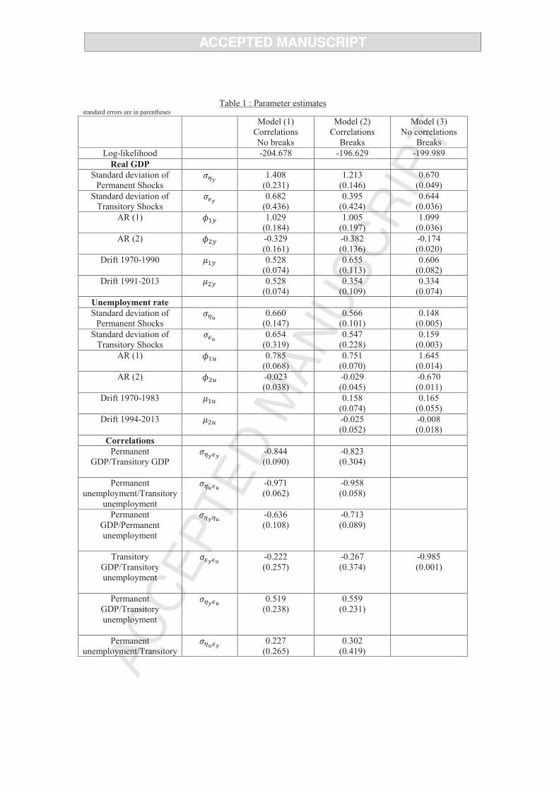
Table 1 : Parameter estimates standard errors are in parentheses

Model (1)

Correlations

No breaks

Model (2)

Correlations

Breaks

Model (3)

No correlations

Breaks

Log-likelihood -204.678 -196.629 -199.989

Real GDP

Standard deviation of

Permanent Shocks !" 1.408

(0.231)

1.213

(0.146)

0.670

(0.049)

Standard deviation of

Transitory Shocks #" 0.682

(0.436)

0.395

(0.424)

0.644

(0.036)

AR (1)

$%& 1.029

(0.184)

1.005

(0.197)

1.099

(0.036)

AR (2) $'& -0.329

(0.161)

-0.382

(0.136)

-0.174

(0.020)

Drift 1970-1990 (%& 0.528

(0.074)

0.655

(0.113)

0.606

(0.082)

Drift 1991-2013 ('& 0.528

(0.074)

0.354

(0.109)

0.334

(0.074)

Unemployment rate

Standard deviation of

Permanent Shocks !) 0.660

(0.147)

0.566

(0.101)

0.148

(0.005)

Standard deviation of

Transitory Shocks #) 0.654

(0.319)

0.547

(0.228)

0.159

(0.003)

AR (1)

$%* 0.785

(0.068)

0.751

(0.070)

1.645

(0.014)

AR (2) $'* -0.023

(0.038)

-0.029

(0.045)

-0.670

(0.011)

Drift 1970-1983 (%* 0.158

(0.074)

0.165

(0.055)

Drift 1994-2013 ('* -0.025

(0.052)

-0.008

(0.018)

Correlations

Permanent

GDP/Transitory GDP

!"#" -0.844

(0.090)

-0.823

(0.304)

Permanent

unemployment/Transitory

unemployment

!)#) -0.971

(0.062)

-0.958

(0.058)

Permanent

GDP/Permanent

unemployment

!"!) -0.636

(0.108)

-0.713

(0.089)

Transitory

GDP/Transitory

unemployment

#"#) -0.222

(0.257)

-0.267

(0.374)

-0.985

(0.001)

Permanent

GDP/Transitory

unemployment

!"#) 0.519

(0.238)

0.559

(0.231)

Permanent

unemployment/Transitory !)#" 0.227

(0.265)

0.302

(0.419)

GDP

Figure 1: Unemployment rate and permanent component

Shaded areas are recessions defined by ECRI. Top: Model (2) with correlations and breaks.

Bottom: Model (3) with no correlations and breaks.

Figure 2: Real GDP and permanent component

Shaded areas are recessions defined by ECRI. Top: Model (2) with correlations and breaks.

Bottom: Model (3) with no correlations and breaks.

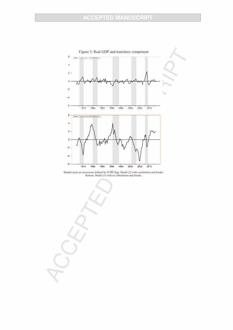
Figure 3: Real GDP and transitory component

Shaded areas are recessions defined by ECRI. Top: Model (2) with correlations and breaks.

Bottom: Model (3) with no correlations and breaks.

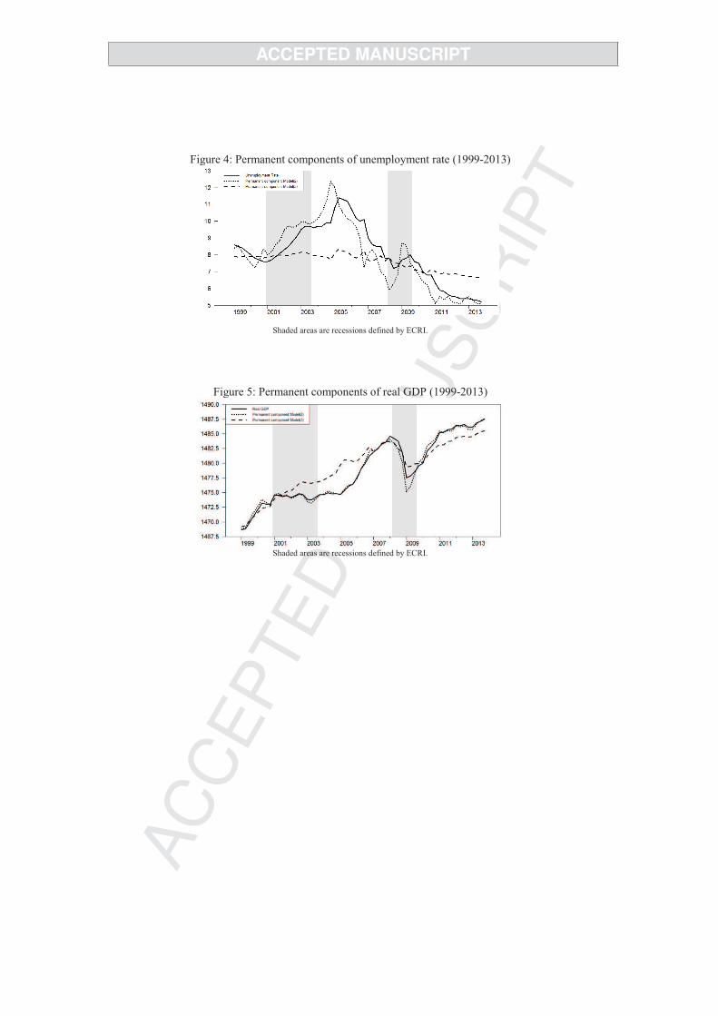
Figure 4: Permanent components of unemployment rate (1999-2013)

Shaded areas are recessions defined by ECRI.

Figure 5: Permanent components of real GDP (1999-2013)

Shaded areas are recessions defined by ECRI.