labor market reforms: an evaluation of the hartz …sarkoups.free.fr/bradleykugler19.pdfmarket e...

Labor Market Reforms:

An Evaluation of the Hartz Policies in Germany

Jake Bradley∗ Alice Kugler†

Abstract

How do workers and firms respond to comprehensive labor market reforms? We use detailed

micro data to analyze the German Hartz Reforms through the lens of a structural model of

the labor market. These reforms aimed at reducing unemployment, by increasing working hour

flexibility, job matching and work incentives. In our setting, reforms directly affect the model

parameters, which are estimated using matched data on 430,000 workers in 340,000 firms. Con-

trary to previous findings, our analysis shows that, although the reforms shortened the typical

duration of unemployment, they did not reduce unemployment as a whole and led to a decline in

wages. Low-skilled workers suffered the most in terms of employment and wage losses. Further-

more, we decompose the contribution of each reform wave to employment and wage changes,

finding that the reduction in generosity of unemployment benefits was the principle driver in

reducing wages.

∗University of

Nottingham

and

IZA,

email:

[email protected].

†University College London, email: [email protected]. We would like to thank the Associate Editor and twoanonymous referees of the journal, as well as Cynthia Doniger, Jan Eeckhout, Joseph-Simon Gorlach, Axel Gottfries,Gregor Jarosch, Hamish Low, Fabien Postel-Vinay and Jean-Marc Robin for helpful suggestions. Seminar partici-pants at the University College London, the University of Cambridge, the University of Bristol, the London School ofEconomics, the RES Inaugural Symposium in Manchester, the Istanbul Search and Matching Workshop, the AnnualSearch and Matching Conference in Amsterdam, the ZEW Summer Workshop, the SAEe in Bilbao, the RES PhDMeetings, the University of Birmingham, the IZA Institute of Labor Economics, Uppsala University, Aarhus Univer-sity, the University of Nottingham and EALE provided useful comments and feedback. We gratefully acknowledgefinancial support by the Keynes Fund under project JHLV.

European Economic Review, Volume 113, April 2019

ACCEPTED MANUSCRIPT

1 Introduction

This paper evaluates the wage and employment impacts of a series of German labor market reforms

using detailed worker-firm micro data. The so-called Hartz reforms were implemented from 2003-

2005 and are particularly difficult to evaluate: they were anticipated, multifaceted in their scope,

likely to have large general equilibrium effects, and were implemented during an expansionary

time for Germany. We build a structural model of the labor market with forward-looking agents

in which the reforms govern the primitive structural parameters of the model. Parameters are

identified through the timing of reform implementations. Using our estimated model we simulate

the impacts of the policies absent other economic changes, so we can isolate the overall effect as

well as individual impacts of specific policies. We find that jointly the policies did not increase

employment but resulted in a reduction of wages of around 4%. This fall in wages is mostly driven

by the reform that reduced the generosity of unemployment benefits. Further, we find that the

decline in wages disproportionally affected low-skilled workers.

The German labor market reforms in the early 2000s are often referred to as exemplary poli-

cies for reducing unemployment. After lackluster economic growth in the 1990s and early 2000s,

Germany outperformed many other industrialized countries from 2006 onwards and during the

Great Recession. Unemployment fell from 12.3% in 1998 to 8.7% in 2008, and Germany attracted

international attention for its transformation from the ‘sick man of Europe to economic superstar’

(Dustmann et al., 2014). However, the extent to which the Hartz reforms altered the performance

of the German labor market, and how they affected unemployment and wages, remains unclear.

In particular, the decrease in unemployment is often attributed to the Hartz reforms. Other less

prominent explanations for the strengthening of the German economy include pre-reform wage

moderation and a favorable export environment. The Hartz reforms consisted of three waves which

were implemented annually from 2003 to 2005. The first wave had the objective of stimulating

labor demand, mostly through tax breaks for part-time work. The second reform wave aimed at

improving labor market efficiency through better matching of workers and firms, and the final wave

introduced a series of supply-side policies that disincentivized unemployment.

1

Our paper contributes to an extensive literature on the link between the rigidity of labor market

institutions, unemployment and wages. In the context of the German Hartz reforms, two types

of studies exist that investigate specific subsets of the reform policies. A number of structural

macroeconomic papers explicitly model certain reform aspects (for example, Krause and Uhlig,

2012; Krebs and Scheffel, 2013; Launov and Walde, 2013, 2016), and find declines of unemployment

in response to the second and third reform waves that vary in size, and mixed evidence on wages.

Typically these papers are calibrated or estimated using pre-reform data and explicitly model spe-

cific reform features. On the other hand, reduced-form approaches use discontinuities or structural

breaks to analyze specific reform policies (for instance, Fahr and Sunde, 2009; Klinger and Rothe,

2012; Hertweck and Sigrist, 2013; Price, 2018; Tazhitdinova, 2018). These studies broadly indicate

small declines in unemployment in response to each of the Hartz policies. Our paper differs from

these papers by exploiting detailed micro data for evaluating the effects of the Hartz policies jointly

in the presence of interacting labor market institutions. By imposing structure on the data gener-

ating process, we provide insights into the mechanisms and outcomes of Germany’s transition to a

more flexible labor market.

Our work builds on the literature of labor market equilibrium models and in particular on the

sequential auction model in Postel-Vinay and Robin (2002). In our framework, wage determination

is tractable out of steady-state as in Postel-Vinay and Turon (2010) and Lise and Robin (2017).

We extend the framework in Lise and Robin (2017) by including a match-specific component, a

wage setting mechanism that can replicate the empirical wage distribution, and shocks that affect

the parameter space rather than labor productivity. Equilibrium labor market models with search

frictions are used to evaluate specific policies (for example, Bentolila et al., 2012; Bradley et al., 2017;

Shephard, 2017), but this methodology cannot be easily expanded for investigating labor market

reforms with extensive scope or when policies lack a clear evaluation metric. In a similar approach

to our paper, Murtin and Robin (2018) develop and estimate a structural model of labor markets,

with changes in policies as reduced-form effects on the structural parameters.1 Their model focuses

1This structural and reduced-form hybrid approach is not new. In the discrete choice literature the approach was

pioneered by Keane and Moffitt (1998), and more recently, Blundell and Shephard (2012) model the stigma associated

2

on employment and its volatility, and is estimated for nine OECD countries. Dispersion in labor

market policies across these countries maps to differences in structural parameters. By contrast,

our paper identifies changes in parameters from the timing of policy reforms within a single country,

with policy effects on the distribution of wages in addition to employment.

This paper is organized as follows. Section 2 provides an overview of the Hartz reforms, summa-

rizes the evolution of employment and wages over the reform periods, and motivates our conceptual

approach. Section 3 describes the model. The estimation protocol is presented in Section 4. Section

5 discusses the estimation results and simulates the model to uncover the reform impacts on wages

and employment. Section 6 concludes.

2 The Hartz Reforms

The Hartz reforms consist of four labor market reform laws that were implemented in Germany be-

tween 2003 and 2005. The main objective of the reforms was to reduce unemployment. To reach this

objective the reforms included extensive changes for workers and firms, such as increased working

hour flexibility, improved job matching, and more stringent work incentives for the unemployed.

The Hartz laws were based on suggestions by the Commission for Modern Services in the Labor

Market, also called the Hartz Commission. After years of rising unemployment, labor market policy

was a central issue in the German elections in 1998 and 2002. When unemployment remained high,

the Hartz Commission was appointed on February 22nd 2002 in response to a scandal, which revealed

that the Federal Employment Agency had significantly embellished the numbers of successfully

placed job seekers. The Hartz Commission was composed of 15 experts from industry, politics and

academia, and named after the chairman of the Commission, Peter Hartz, who was an executive in

charge of personnel at Volkswagen at the time. The Commission published its suggestions for labor

market policy changes in August 2002. These suggestions led to the Hartz reform package, which

was implemented from January 1st 2003 onwards. Table 1 gives an overview of the timing and

content of the Hartz I-IV laws, and Appendix A.1 provides more details on the reform contents.

with welfare take-up and Attanasio et al. (2012) evaluate the impact of transfers on the marginal utility of income.

3

Broadly summarized, the first wave aimed at raising labor demand, the objective of the second

wave was to improve labor market efficiency, and the final wave was targeted at increasing labor

supply.

Table 1: The Hartz Reforms

Announcement: February 22nd 2002

- The Hartz Commission is appointed to suggest labor market reforms.

Labor demand: Hartz I & II laws, taking effect on January 1st 2003

- Hiring of temporary workers is made easier.

- Continued training is subsidized with vouchers.

- Tax exemption thresholds are increased for mini- and midi-jobs, from April 1st on.

- Subsidies for startups by the unemployed are introduced.

Market efficiency: Hartz III law, taking effect on January 1st 2004

- The Federal Employment Agency is restructured to improve service delivery and job

placement of the unemployed.

Labor supply: Hartz IV law, taking effect on January 1st 2005

- The long-term unemployed receive less support, now in the form of a flat-rate payment.

- Unemployment benefit receipt is made further contingent on asset-based means testing.

- Sanctions are introduced for the refusal of job offers.

The Hartz I and II reforms came into effect on January 1st 2003. Hartz I, the first of the four

‘Laws for Modern Services in the Labor Market’, facilitated temporary employment and introduced

new training subsidies. Hartz II further regulated marginal employment, so-called mini- and midi-

jobs, and sponsored business startups by the unemployed. Mini-jobs provided tax exemption of

worker contributions to social security and lifted the threshold for such marginal tax-exempt em-

ployment from a monthly income of 325 to 400 Euros. Midi-jobs incurred reduced social security

contributions on a sliding scale for earnings up to 800 Euros per month. The definition of marginal

employment was also extended to employees working more than 15 hours per week. As a result

of Hartz II, the number of workers holding a mini-job as their main employment increased from

around 13% in 2003 to 16% in 2006, and additionally over 4% of workers engaged in mini-jobs as a

4

second job and more than 3% of workers held midi-jobs by 2006 (Galassi, 2017). The third reform

law, Hartz III, was implemented from January 1st 2004, and restructured the Federal Employment

Agency with the objective of making it a modern, client-oriented service provider. Hartz IV came

into effect on January 1st 2005, and was one of the most extensive and controversial labor market re-

forms that was ever implemented in Germany. It significantly changed the structure and generosity

of unemployment receipts, by combining unemployment assistance for the longer-term unemployed

with social assistance into a flat-rate payment, and introducing sanctions to promote more active

job search. The effects of Hartz IV for payments received by the unemployed were ambiguous. For

example, households with low incomes in employment and single-parent households profited from

the reform, while those with higher employment incomes experienced a reduction of benefits (Koch

and Walwei, 2005). A separate law in January 2005 specified reductions of unemployment benefit

durations, which we do not analyze in this paper. These reductions in benefit duration were applied

to unemployment spells starting from February 2006 on, with the first duration cuts in effect only

in 2007.

2.1 The Reform Effects

To examine the impact of the Hartz reform laws, we use data on 430,000 males working in 340,000

firms from the Sample of Integrated Labor Market Biographies (SIAB) between 2001 and 2005. The

data are stratified into three skill groups. Workers with an intermediate school leaving certificate or

less are defined as low-skilled, workers with a vocational qualification such as an apprenticeship and

with an upper secondary school certificate are combined in a medium-skill group, and university

graduates are classified as high-skill workers.

2.1.1 Employment

Figure 1 plots the aggregate unemployment rate of Germany between 2000 and 2007. The dates of

the announcement and implementations of the Hartz reforms are denoted by vertical dashed and

solid lines respectively.

5

Figure 1: Unemployment rate 2000-2006

Notes: The unemployment rate displayed is for the share unemployed of employees covered

by social insurance, and is provided by the Bundesagentur fur Arbeit.

As shown in Figure 1, unemployment increases during the implementation of the reforms be-

tween 2003 and 2005 and falls after the Hartz IV law comes into force in 2005. The increase in

unemployment is already visible from the initial announcement of reforms after the appointment

of the Hartz Commission in February 2002. With the implementation of the fourth Hartz law,

unemployment rose to a historical high with over 5.2 million workers unemployed.

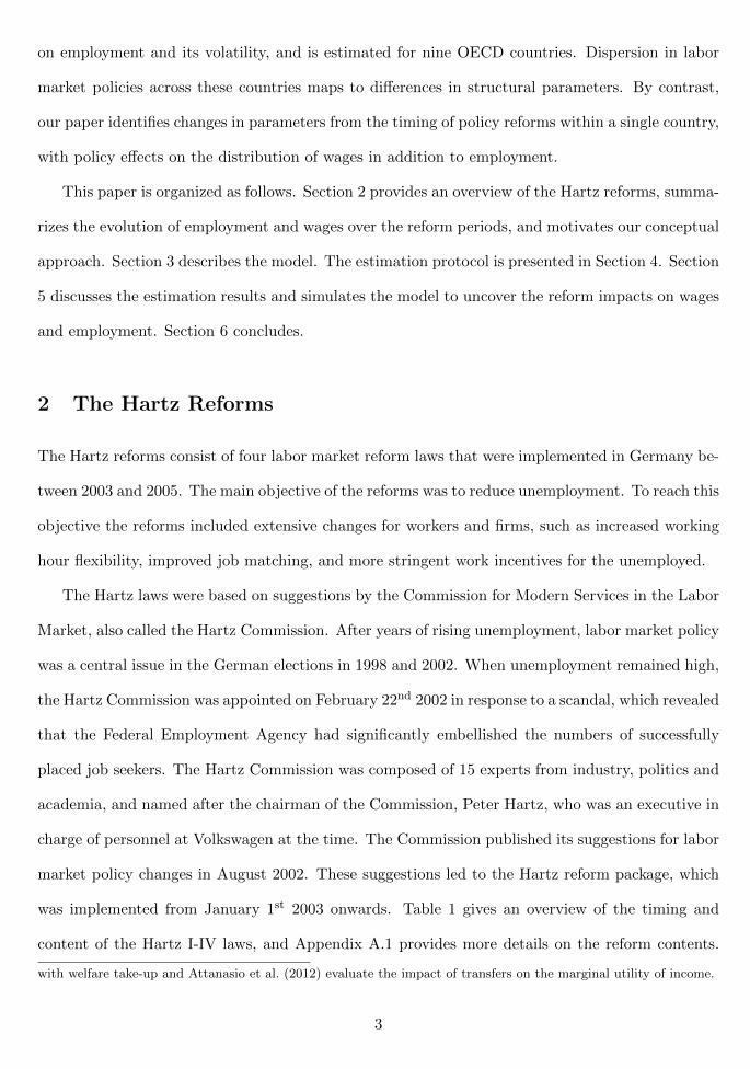
Panel (a) in Figure 2 shows the outflows from unemployment and panel (b) the inflows into

unemployment. All monthly series have been seasonally adjusted using the X-12-Arima program.2

The series indicate that the increased unemployment over the implementation period is primarily

driven by a fall in the job finding rate, and the post-reform decrease in unemployment is associated

with a higher job finding rate. Separation rates increase slightly for the unskilled over the reform

periods. Unskilled workers have the highest separation rates and these remain higher post-2005

compared to the pre-reform period.

2X-12-Arima is a software package developed by the US Census Bureau for seasonally adjusting time series data.

6

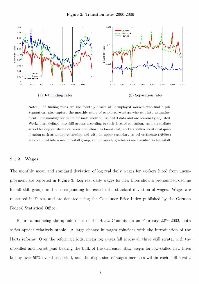
Figure 2: Transition rates 2000-2006

(a) Job finding rates (b) Separation rates

Notes: Job finding rates are the monthly shares of unemployed workers who find a job.

Separation rates capture the monthly share of employed workers who exit into unemploy-

ment. The monthly series are for male workers, use SIAB data and are seasonally adjusted.

Workers are defined into skill groups according to their level of education. An intermediate

school leaving certificate or below are defined as low-skilled, workers with a vocational qual-

ification such as an apprenticeship and with an upper secondary school certificate (Abitur)

are combined into a medium-skill group, and university graduates are classified as high-skill.

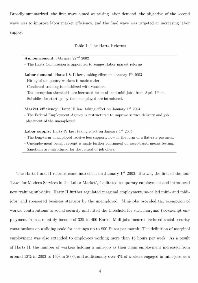
2.1.2 Wages

The monthly mean and standard deviation of log real daily wages for workers hired from unem-

ployment are reported in Figure 3. Log real daily wages for new hires show a pronounced decline

for all skill groups and a corresponding increase in the standard deviation of wages. Wages are

measured in Euros, and are deflated using the Consumer Price Index published by the German

Federal Statistical Office.

Before announcing the appointment of the Hartz Commission on February 22nd 2002, both

series appear relatively stable. A large change in wages coincides with the introduction of the

Hartz reforms. Over the reform periods, mean log wages fall across all three skill strata, with the

unskilled and lowest paid bearing the bulk of the decrease. Raw wages for low-skilled new hires

fall by over 50% over this period, and the dispersion of wages increases within each skill strata.

7

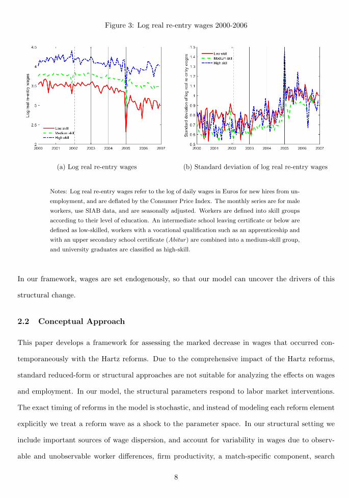
Figure 3: Log real re-entry wages 2000-2006

(a) Log real re-entry wages (b) Standard deviation of log real re-entry wages

Notes: Log real re-entry wages refer to the log of daily wages in Euros for new hires from un-

employment, and are deflated by the Consumer Price Index. The monthly series are for male

workers, use SIAB data, and are seasonally adjusted. Workers are defined into skill groups

according to their level of education. An intermediate school leaving certificate or below are

defined as low-skilled, workers with a vocational qualification such as an apprenticeship and

with an upper secondary school certificate (Abitur) are combined into a medium-skill group,

and university graduates are classified as high-skill.

In our framework, wages are set endogenously, so that our model can uncover the drivers of this

structural change.

2.2 Conceptual Approach

This paper develops a framework for assessing the marked decrease in wages that occurred con-

temporaneously with the Hartz reforms. Due to the comprehensive impact of the Hartz reforms,

standard reduced-form or structural approaches are not suitable for analyzing the effects on wages

and employment. In our model, the structural parameters respond to labor market interventions.

The exact timing of reforms in the model is stochastic, and instead of modeling each reform element

explicitly we treat a reform wave as a shock to the parameter space. In our structural setting we

include important sources of wage dispersion, and account for variability in wages due to observ-

able and unobservable worker differences, firm productivity, a match-specific component, search

8

frictions, and sorting across all these dimensions.

A reduced-form evaluation that compares outcomes before and after the implementation of

a specific policy is not feasible in the context of the Hartz reforms. It is likely that firms and

workers anticipated the Hartz policy changes before the implementation of the reform policies and

adjusted their behavior before the first Hartz reform and until Hartz IV took effect. A reduced-form

assessment may also fall short because of the persistence of the endogenous variables, employment,

and wages. An alternative approach would impose full structure on the data generating process

and specify each policy explicitly in a structural model. The Hartz reforms, however, lack clear

evaluation metrics and were so wide-ranging that it is not feasible to model all the different reform

features.

Furthermore, we assess the impacts of the Hartz reform waves in isolation. To mitigate the

effects of contemporaneous macroeconomic developments, we restrict our estimation to a relatively

short time period and subtract a trend component in the moments used for identification. As a

result, our results can be interpreted as the impact of the Hartz reforms net of other macroeconomic

trends.

3 The Model

3.1 The Environment

Time is continuous and denoted by t, where t ∈ R+. Parameters subscripted by t vary over time,

and θt denotes the vector of parameters at time t. The structural parameters of the model evolve

according to a jump process that occurs at the instance of the introduction of each labor market

reform wave. Changes to θt are fully anticipated by the agents, but in order to keep the problem

stationary, the exact instance at which the policy is implemented is not known. Instead, risk neutral

agents know the instantaneous probability that a policy will be implemented. The Poisson rate ηt

is calibrated to match the frequency of the Hartz reforms. Assuming that agents do not know the

exact implementation dates makes the setting tractable. Instead of an infinite number of states, at

any point in time the Poisson process ensures only five possible states between the announcement

9

and implementations of individual policy, as described in Section 2.

The labor market consists of a continuum of infinitely lived workers of mass one, who are

indexed by their level of productivity x ∈ (x, x). Workers can either be employed or unemployed,

and the measure of workers of productivity x is given by `(x). When a worker is unemployed he

receives a flow utility value bt(x). A continuum of firms exist that are indexed by their productivity

y ∈ (y, y). When a worker is hired by a firm, the amount produced depends on the productivities

of the worker and the firm as well as on a match-specific draw, z ∈ (z, z). The match-specific

component z is drawn from a known distribution with density γ(z), which is independent of worker

and firm productivities. The decision whether to form a match is made after the realization of z.

A worker and firm of productivity x and y with a match-specific productivity draw z produce an

amount ft(x, y, z), where ft : (x, x)× (y, y)× (z, z)→ R+. Our initial assumption for the functional

form of ft(x, y, z) is that as z → z, ft(x, y, z)→∞.

The economy is characterized by search frictions and workers cannot observe the full menu of

jobs. Instead job offers arrive randomly to a worker at time t with an exogenous Poisson arrival rate

λ0,t if the worker is unemployed and λ1,t if the worker is employed. The sampling density of firms

is fixed over time and given by υ(y). Jobs are destroyed at an exogenous rate δt, after which the

worker becomes unemployed. Without loss of generality, the sampling densities `(x), υ(y) and γ(z)

are parameterized as uniform on [0, 1], thus x, y and z can be thought of as productivity ranks. It

is isomorphic to think about Hartz policy as directly impacting ft(·) or the primitive distributions

of types.

3.2 Wage Determination

Wage contracts are re-negotiated sequentially as in the sequential auction model, pioneered by

Postel-Vinay and Robin (2002). For an unemployed worker, wages are determined as in Cahuc

et al. (2006) and Dey and Flinn (2005), where a firm hires a worker from unemployment and the

worker and firm split the surplus. The worker receives a fraction β of the generated surplus and

the firm receives the rest. When a worker is employed, however, wages are determined as in Postel-

10

Vinay and Robin (2002), where on the job search triggers Bertrand competition between a worker’s

current employer and the poaching firm. If the unemployed worker’s bargaining power β were equal

to zero, then wages are determined as in Postel-Vinay and Robin (2002). We modify the model

setup in Postel-Vinay and Robin (2002) to ensure that wage offers taken by the unemployed are

well-behaved, which is important for our identification argument. In a standard Postel-Vinay and

Robin (2002) wage protocol our model cannot generate sufficiently high starting wages, and wages

offered to an unemployed worker would be decreasing in the productivity type of a firm.

We remain agnostic with respect to the effects of a policy shock on wages, and our setup

can accommodate a variety of protocols with varying degree of wage rigidity. To make as few

assumptions as possible, in the estimation wages are only targeted as an empirical moment in

steady-state, before the announcement of the reform. In Appendix A.2 we outline one of several

potential ways to model the wage re-negotiation process after a policy shock. Since wage re-

negotiation after policy shocks is ambiguous in our setting, we are limited to pre- and post-reform

comparisons of the economy’s steady-states in evaluating the policy impact on wages.

For a given wage w, the surplus is shared between the worker and the firm. Wt(·) denotes the

value function of an employed worker, Ut(·) is the value function of an unemployed worker, Πt(·) is

the value function of a firm that hires a worker, and St(x, y, z) is the total surplus generated by a

match.

Wt(w, x, y, z)− Ut(x) + Πt(w, x, y, z) = St(x, y, z) (1)

It is assumed that the outside option of the firm is zero. The wage provides an unemployed

individual with an additional value equal to βSt(x, y, z). The wage of a worker’s first job after

leaving unemployment is a function of his productivity, the firm’s productivity and the match-

specific draw, and denoted by φ0,t(x, y, z). If a positive surplus is generated then it is in the interest

of the worker and the firm to form a match. Thus the values of y and z that result in matches for

the worker are a function of his own productivity x and given by M0,t(x) ≡ {y, z|St(x, y, z) ≥ 0}.

The wage solves the following equality:

Wt(φ0,t(x, y, z), x, y, z)− Ut(x) = βSt(x, y, z). (2)

11

3.3 Wage Mobility

When a firm meets an employed worker, the poaching firm draws a match-specific productivity

that is observable to all parties. The incumbent and the poaching firm then engage in Bertrand

competition to hire or retain the worker. For a worker of productivity x employed in a firm of

productivity y with match-specific productivity z, three possible things can happen.

Move jobs: The worker moves if the surplus generated from the poaching firm is greater than

the current surplus generated. The set of poaching firm and match-specific productivities y′,

z′ is given by M1,t(x, y, z) ≡ {y′, z′|St(x, y′, z′) ≥ St(x, y, z)}. Due to asymmetries in the

wage bargaining process between employed and unemployed workers the determination of the

new wage remains ambiguous. We therefore partition M1,t(x, y, z) into M10,t(x, y, z) and

M11,t(x, y, z), where, M1,t(x, y, z) = {M10,t(x, y, z) ∪M11,t(x, y, z)}.

The more familiar case is when new offers (y′, z′) are in the set M11,t(x, y, z) and the set is

defined as M11,t(x, y, z) ≡ {y′, z′|St(x, y′, z′) ≥ St(x, y, z) ≥ βSt(x, y′, z′)}. In this instance

the worker moves to the new firm and uses his current employment as his outside option in

Bertrand competition. The new wage of the worker is given by equation (3) and he is able to

extract all the surplus from his former match.

Wt(φ1,t(x, y′, z′, y, z), x, y′, z′)− Ut(x) = St(x, y, z) (3)

If the difference in surplus generated between the poaching firm and the incumbent firm, how-

ever, is sufficiently large, and (y′, z′) ∈M10,t(x, y, z) andM10,t(x, y, z) ≡ {y′, z′|βSt(x, y′, z′) >

St(x, y, z)}, then the worker gets a larger share of the surplus if he uses unemployment as his

outside option. After meeting a higher surplus match, the worker instantaneously quits his

current job and bargains with the poaching firm as an unemployed agent. The worker’s new

wage is defined in equation (2).

Stay in the same job with a wage increase: The worker receives a within-firm promotion

if the surplus generated by a new offer is high enough to trigger Bertrand competition with the

12

incumbent firm but not higher than the surplus of the current match. Bertrand competition is

triggered if the surplus of a new match is greater than the worker surplus in the current match.

Formally, the set of y′, z′ is defined as M2,t(w, x, y, z) ≡ {y′, z′|St(x, y, z) > St(x, y′, z′) >

Wt(w, x, y, x)− Ut(x)}. The worker’s new wage solves the equality:

Wt(φ1,t(x, y, z, y′, z′), x, y, z)− Ut(x) = St(x, y

′, z′).

No change: If a worker receives an offer that generates less surplus than he is already taking

from his current match, then the incumbent firm does not need to offer a higher wage to

retain the worker. The set of y′, z′ is defined as (y′, z′) \ {M1,t(x, y, z) ∪M2,t(w, x, y, z)}.

3.4 The Surplus

This class of models has the advantage that only the expression that defines the surplus needs to

be solved. By contrast, solving for the worker and firm individual value functions would involve

five (rather than three) continuous variables. Further, worker and firm value functions would

require specific assumptions about the way in which wages are re-negotiated after a policy shock.

The surplus function is given by equation (4) and is formally derived in Appendix A.3. The +

superscript denotes A+ := max{A, 0}.

(r + δt+ηt)St(x, y, z) = ft(x, y, z)− bt(x)− βλ0,t∫ ∫

St(x, y′, z′)+υ(y′)γ(z′)dy′dz′

+ λ1,t

∫ ∫ [βSt(x, y

′, z′)− St(x, y, z)]+υ(y′)γ(z′)dy′dz′ + ηtSt′(x, y, z)

+ (4)

Equation (4) describes the surplus generated by a match and is the fundamental equation of the

model. It dictates the decisions of agents about who to match with and determines the resulting

wages from consummating the match. The surplus consists of the net gain in flow utility, output

minus home production, and three option values. The first integral term is the option premium

in unemployment, the value of future employment to the unemployed. We refer to the second

integral term as the quit premium, which is the additional surplus generated by being able to use

unemployment as a worker’s outside option. Since this expression is non-negative, it increases the

13

total number of feasible matches. The final term represents the agent’s expectations about the

time-varying parameters after a shock. If future parameters, θt′ generate more (less) surplus than

the current parameters this adds (reduces) value to the current surplus and further encourages

(deters) realizing a match today.

We solve equation (4) numerically. Since the surplus at t depends on the surplus at t′, it

is solved by backward induction.3 Furthermore, one does not need to form expectations about

the value of the future surplus because the policy implications are anticipated. The deterministic

nature of the policy interventions is far simpler to deal with computationally, and it is not obvious

how to calibrate an alternative distribution of beliefs about future policy. Agents’ perfect foresight

over policy therefore seems a reasonable assumption to make. An additional computational burden

arises due to the quit premium. Unlike the option value of unemployment, the set M10,t(x, y, z)

over which we integrate is a function of y and z. Under the majority of parameterizations that we

have experimented with, however, this constitutes a relatively small share of total surplus and it

thus is computationally more efficient not to update this term at every iteration.

Lemma 1 As z → z, St(x, y, z)→∞.

Lemma 1 is proved in Appendix A.4.1.

Proposition 1 The set,

Mxyt ≡

{x, y|

∫ z

z1{St(x, y, z) ≥ 0}γ(z)dz > 0

}

is equal to the universe of (x, y), that isMxyt : (x, x)× (y, y).

Proposition 1 is proved in Appendix A.4.2. The set of all feasible worker-firm matches at time t

is given by Mxyt . The fact that this set covers the universe of (x, y) suggests that all worker-firm

pairs are feasible. No worker-firm match observed empirically can be used to falsify the model.

Lemma 2 For any x, y, y′ and z′, there is a z such that St(x, y, z) > St(x, y′, z′).

Lemma 2 is proved in Appendix A.4.3.

3Solving by backward induction relies upon the final state being absorbing. After Hartz IV it is assumed that

agents anticipate no further reforms, and ηt = 0 at a time t that is sufficiently large, as described in Section 3.6.

14

Proposition 2 The set

My−1,t (x, y, z) ≡ {y′, z′|St(x, y′, z′) ≥ St(x, y, z) ∩ y > y′}

is non-empty for all (x, y, z).

Proposition 2 follows directly from Lemma 2. In equilibrium any employed agent may volun-

tarily move to a less productive firm. We use the type of job mobility defined in Proposition 2 as

an identification argument for the variation in the match-specific component z.

3.5 Wage Equations

In order to impose as little structure on the wage setting mechanism as possible, wages are only

defined in stable periods, when ηt = 0. The wage a worker receives depends on whether he has

any outside options in employment. The outside option affects the current wage either because

the worker moved from one employer to another or because he received sufficiently good job offers

while with his current employer. Equation (5) represents the wage of a worker of type x in a firm

of type y and a match-specific draw of z with no outside options. This case arises for all workers

who join a firm from unemployment.

φ0,t(x, y, z) =ft(x, y, z)− (1− β)(r + δt + ηt)St(x, y, z)

− (1− β)λ1,tSt(x, y, z)

∫ ∫

y′,z′∈M1,t(x,y,z)υ(y′)γ(z′)dy′dz′

− λ1,t∫ ∫

y′,z′∈M2,t(x,y,z)[St(x, y

′, z′)− βSt(x, y, z)]υ(y′)γ(z′)dy′dz′ (5)

Equation (5) is derived by solving the equality given by equation (2). This derivation and the

formal definitions of the integral supports are provided in Appendix A.5.

A worker of type x in a firm of type y′ with match-specific draw z′ who previously received an

offer from a firm of type y with match-specific draw z receives a wage given by equation (6). This

wage is derived by solving the equality given by equation (3). The derivation and the definition of

15

all sets are given in Appendix A.6.

φ1,t(x, y, z, y′,z′) = ft(x, y

′, z′)

− λ1,t∫ ∫

y′′,z′′∈M11,t(x,y,z)[St(x, y, z)− St(x, y′, z′)]υ(y′′)γ(z′′)dy′′dz′′

− λ1,t∫ ∫

y′′,z′′∈M2,t(x,y,z)[S(x, y′′, z′′)− S(x, y′, z′)]υ(y′′)γ(z′′)dy′′dz′′ (6)

Proposition 3 The set

Mw−1,t (w, x, y, z) ≡ {y′, z′|St(x, y′, z′) ≥ St(x, y, z) ∩ φ1,t(x, y′, z′, y, z) < w}

is non-empty for some (t, w, x, y, z).

Bertrand competition between employers for employed workers retains the attractive feature

of Postel-Vinay and Robin (2002) that some employment transitions are associated with a wage

cut. The worker accepts a wage cut because he is sufficiently compensated by the increase in the

option value of future job offers. The proof for this mechanism is provided in Appendix A.7. Since

Proposition 2 is for all (x, y, z) the set Mw−1,t (w, x, y, z) defined above can be partitioned further,

by conditioning on an increase or decrease in firm productivity. In this way, the model is able to

generate any com bination of increase or decrease in wage or firm productivity.

3.6 Labor Dynamics

Rather than modeling the specifics of each reform package, we implement the Hartz policy waves

as a series of shocks to the structural parameters of the model. The impact of each reform package

on the parameter space is fully anticipated. At time t agents believe policies arrive at a Poisson

arrival rate ηt. This model feature is somewhat unrealistic because agents are likely to know the

exact date of the reform in the immediate lead up to a policy implementation. Since in our setup

agents are risk neutral, however, uncertainty over the exact timing of the policy is not important.

Furthermore, before the formation of the Hartz Commission on February 22nd 2002 and after the

implementation of Hartz IV on January 1st 2005, agents believe the parameter space is stable

indefinitely. In these two stable periods, the probability that the parameter space changes is zero,

16

ηt = 0. Therefore, from equation (4) the value of the surplus in a match (x, y, z) at time t is equal

to the value of the surplus in the same match for any t′ > t.

The two stable periods can be solved for independently of the evolution of the structural pa-

rameter set before or after the reforms. There are three periods when agents anticipate further

changes to the parameter set, which we refer to as the unstable periods. These unstable periods

take place after the announcement but before implementation of Hartz I and II, after Hartz I and II

but before Hartz III, and after Hartz III but before Hartz IV. In the unstable periods, the surplus

generated of a match today depends on how the structural parameters evolve in the future. These

structural parameters are solved for sequentially by backward induction.

In the first stable period before the reforms were anticipated the distribution of unobservables

(x, y, z) among matched agents or the distribution of worker type (x) among the unemployed are

unclear. The initial allocation of worker, firm and match types is consequential for the effects of the

reforms. For simplicity we therefore assume that the economy is in steady-state before the reform

is announced in February 2002, which seems reasonable because the last recession in Germany

occurred almost a decade earlier in 1993. The initial allocation of workers and firms is derived in

Appendix A.8.

3.6.1 Labor Adjustment

A series of shocks to the parameter space are realized, corresponding to the initial announcement

of the reforms and the subsequent reform implementations. At the incidence of the ith shock, at t

equal to ti, an instantaneous adjustment in labor assignment takes place. All matches that generate

negative surplus after the new realization of the parameter space are separated. Time t−i denotes

the time immediately before ti. Formally, t−i is given by t−i = limε→0−

(ti + ε). Equation (7) shows

the immediate readjustment of the measure of unemployment.

uti(x) = ut−i(x) +

∫ ∫

y′,z′ /∈M0,ti(x)et−i

(x, y′, z′)dy′dz′ (7)

The first term represents the unemployed from the previous period and the second term are the

employed agents who no longer generate a positive surplus after the new realization of the parameter

17

space in ti. The pre-shock measure of employed individuals in period ti of productivity x in firm

y with match-specific component z is conditional on positive surplus still being generated, and

expressed in equation (8).

eti(x, y, z) = {Sti(x, y, z) ≥ 0}et−i (x, y, z) (8)

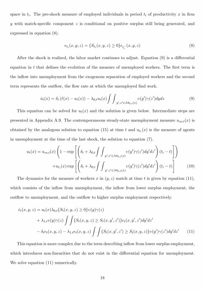
After the shock is realized, the labor market continues to adjust. Equation (9) is a differential

equation in t that defines the evolution of the measure of unemployed workers. The first term is

the inflow into unemployment from the exogenous separation of employed workers and the second

term represents the outflow, the flow rate at which the unemployed find work.

ut(x) = δt (`(x)− ut(x))− λ0,tut(x)

∫ ∫

y′,z′∈M0,t(x)υ(y′)γ(z′)dydz (9)

This equation can be solved for ut(x) and the solution is given below. Intermediate steps are

presented in Appendix A.9. The contemporaneous steady-state unemployment measure uss,t(x) is

obtained by the analogous solution to equation (15) at time t and uti(x) is the measure of agents

in unemployment at the time of the last shock, the solution to equation (7).

ut(x) = uss,t(x)

(1− exp

[(δt + λ0,t

∫ ∫

y′,z′∈M0,t(x)υ(y′)γ(z′)dy′dz′

)(ti − t)

])

+uti(x) exp

[(δt + λ0,t

∫ ∫

y′,z′∈M0,t(x)υ(y′)γ(z′)dy′dz′

)(ti − t)

](10)

The dynamics for the measure of workers x in (y, z) match at time t is given by equation (11),

which consists of the inflow from unemployment, the inflow from lower surplus employment, the

outflow to unemployment, and the outflow to higher surplus employment respectively.

et(x, y, z) = ut(x)λ0,t{St(x, y, z) ≥ 0}υ(y)γ(z)

+ λ1,tυ(y)γ(z)

∫ ∫{St(x, y, z) ≥ St(x, y′, z′)}et(x, y′, z′)dy′dz′

− δtet(x, y, z)− λ1,tet(x, y, z)∫ ∫

{St(x, y′, z′) ≥ St(x, y, z)}υ(y′)γ(z′)dy′dz′ (11)

This equation is more complex due to the term describing inflow from lower surplus employment,

which introduces non-linearities that do not exist in the differential equation for unemployment.

We solve equation (11) numerically.

18

3.7 Solution of the Model

The solution to the surplus of a match, the wages of a given match, and the distribution of matches

in the economy define the solution of the model. The surplus of a match defined by equation

(4) establishes the sets of feasible matches and job switches, M0,t(x) and M1,t(x, y, z). From

the surplus equation, the wage paid in a given match can be solved explicitly, which is given by

φ0,t(x, y, z) and φ1,t(x, y, z, y′, z′) depending on types and outside offers. Finally, the flow equations

from the previous subsection define the distribution of different matches at time t: ut(x), et(x, y, z),

and et(x, y, z, y′, z′). Further details of how the model is solved computationally are provided in

Appendix A.10.

4 Data and Estimation

This section describes our construction of macroeconomic time series for the German labor market,

and how we parameterize, identify and estimate the model. We provide details about the data

generating process, the likelihood function, and the fit of the parameter estimates in matching the

time series. The model is simulated so it matches the data series from January 2001, over 13 months

before the formation of the Hartz Committee, until the end of 2006, 12 months after the final wave

of reforms. For estimating we split the data into a pre-reform period from January 2001 to January

2002, an announcement period from February to December 2002, the implementation of Hartz I

and II from January to December 2003, the implementation of Hartz III from January to December

2004, the implementation of Hartz IV from January to December 2005, and a post-reform period

from January to December 2006.

Instead of just the permanent worker type x, we further distinguish skill by observable worker

skill characteristics. Assuming a segmented labor market we stratify the sample and estimate the

model by skill group, indexed by k. Our data includes information on eight skill levels that we use

to allocate workers into three skill groups. Workers with an intermediate school leaving certificate

or below are defined as low-skilled, workers with a vocational qualification such as an apprenticeship

19

and with an upper secondary school certificate (Abitur) are combined into a medium-skill group,

and university graduates are classified as high-skill. For observations with missing skill information,

we impute the skill group by following the IP1 procedure in Fitzenberger et al. (2006), which for a

given worker interpolates skill information when it is missing.

The model presented in the previous section is fully parameterized and we estimate the struc-

tural parameters. Our assumptions about the data generating process make an analytically tractable

likelihood function feasible. Our approach to maximize a likelihood function makes inference signif-

icantly more straightforward than more typical estimations by the method of moments or indirect

inference.

4.1 The Data

To examine the impact of the Hartz reforms we use the Sample of Integrated Labor Market Bi-

ographies (SIAB), a German worker-firm dataset. The SIAB is a 2% random sample drawn from

administrative data and links information on workers from German administrative data with firm

information from the Establishment History Panel. We restrict the estimation sample to male full-

and part-time workers between the age of 20 and 60, who are not in vocational training. This

choice of age group means most individuals in the sample have finished their education and are

working. Individual daily employment spell data are available from administrative data for employ-

ees covered by social security. Around 80% of the German labor force are covered by compulsory

social security contributions, which exclude the self-employed, public sector workers and military

employees. The SIAB also includes workers that are registered as unemployed but does not provide

information on out-of-the-labor-force status. Our paper focuses on men only due to the lack of

data on labor market transitions from non-participation, which disproportionately affect women.

Including women in the estimation sample would likely lead to more pronounced effects of the Hartz

II reform on wages, as women account for a larger share of the take-up of mini- and midi-jobs. Data

access to the SIAB was provided via on-site use at the Research Data Centre of the German Federal

Employment Agency at the Institute for Employment Research (IAB) and subsequently by means

20

of remote data access.

We use a conservative measure of unemployment, which includes only recipients of benefits

or assistance payments who worked before becoming unemployed but not other job seekers. This

measure of unemployment is consistent over time but is lower than the officially recorded number of

unemployed by construction. It has the advantage of reducing the effect of a spike in unemployment

in January 2005 that is largely due to a change in measuring unemployment that required previous

recipients of social assistance to register as unemployed (Bundesagentur fur Arbeit, 2005).4 Cru-

cially, this allows us to keep a consistent definition of unemployment across our estimation window

that is unaffected by the reclassification in 2005.

The mean of daily real wages for employed workers in our sample is 74.24 Euros and 49.72 Euros

for newly hired workers who re-enter employment. Unemployed workers receive an average daily

benefit payment of 33.42 Euros. Low-skill workers with an average wage of 53.70 Euros account

for 10% of observations, 76% of workers are medium-skill with an average wage of 70.80 Euros and

14% are high-skill workers earning an average wage of 108.26 Euros. The sizes of the three skill

groups are relatively constant, with some decline in the number of low- and medium-skill workers

and a small increase of high-skill workers. The number of workers and the proportion of top-coded

wages by skill group are reported in Table 2.

Table 2: Number of workers and share of top-coded wages by skill group

Number of workers Share top-coded Share re-entry top-coded

Year S1 S2 S3 S1 S2 S3 S1 S2 S3

2001 36,583 267,027 46,201 0.005 0.054 0.384 0.004 0.048 0.328

2002 35,701 263,822 46,729 0.005 0.053 0.387 0.004 0.048 0.329

2003 35,145 264,046 46,977 0.002 0.033 0.299 0.002 0.030 0.257

2004 34,765 262,102 47,182 0.002 0.034 0.304 0.002 0.030 0.263

2005 36,187 262,305 47,599 0.002 0.033 0.303 0.002 0.030 0.263

Notes: S1, S2 and S3 refer to low-skill, medium-skill and high-skill workers respectively.

4The differences between alternative measures and data sources for unemployment in Germany are discussed in

Hertweck and Sigrist (2013) and Rothe and Walde (2017).

21

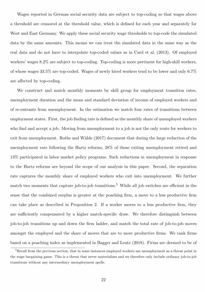
Wages reported in German social security data are subject to top-coding so that wages above

a threshold are censored at the threshold value, which is defined for each year and separately for

West and East Germany. We apply these social security wage thresholds to top-code the simulated

data by the same amounts. This means we can treat the simulated data in the same way as the

real data and do not have to interpolate top-coded values as in Card et al. (2013). Of employed

workers’ wages 8.2% are subject to top-coding. Top-coding is more pertinent for high-skill workers,

of whose wages 33.5% are top-coded. Wages of newly hired workers tend to be lower and only 6.7%

are affected by top-coding.

We construct and match monthly moments by skill group for employment transition rates,

unemployment duration and the mean and standard deviation of income of employed workers and

of re-entrants from unemployment. In the estimation we match four rates of transitions between

employment states. First, the job finding rate is defined as the monthly share of unemployed workers

who find and accept a job. Moving from unemployment to a job is not the only route for workers to

exit from unemployment. Rothe and Walde (2017) document that during the large reduction of the

unemployment rate following the Hartz reforms, 28% of those exiting unemployment retired and

13% participated in labor market policy programs. Such reductions in unemployment in response

to the Hartz reforms are beyond the scope of our analysis in this paper. Second, the separation

rate captures the monthly share of employed workers who exit into unemployment. We further

match two moments that capture job-to-job transitions.5 While all job switches are efficient in the

sense that the combined surplus is greater at the poaching firm, a move to a less productive firm

can take place as described in Proposition 2. If a worker moves to a less productive firm, they

are sufficiently compensated by a higher match-specific draw. We therefore distinguish between

job-to-job transitions up and down the firm ladder, and match the total rate of job-to-job moves

amongst the employed and the share of moves that are to more productive firms. We rank firms

based on a poaching index as implemented in Bagger and Lentz (2018). Firms are deemed to be of

5Recall from the previous section, that in some instances employed workers use unemployment as a threat point in

the wage bargaining game. This is a threat that never materializes and we therefore only include ordinary job-to-job

transitions without any intermediary unemployment spells.

22

higher rank the greater is the proportion of hires from employment relative to unemployment. Firm

rank is defined as the share of new hires that are hired from employment, and is measured only for

firms with a total inflow of more than 15 hires. The poaching index πj is constructed as the number

of employees hired from employment Ej over hires from employment and from unemployment Uj

for a firm j:

πj =Ej

Ej + Uj.

Unemployment duration is defined as the number of months a worker has spent in unemployment

since his last employment spell, as recorded in the IAB Benefit Recipient History data. Wages are

reported as log real daily wages in Euros, and are deflated using the yearly Consumer Price Index

from the German Federal Statistical Office. In the case of overlapping or multiple spell observations

for an individual, we use the spell with the highest recorded wage.

As the monthly moment series exhibit marked seasonality for the month of January, we sea-

sonally adjust all series to ensure that policy reforms are not mistaken with seasonal variation

present in the data. To adjust for seasonal variation from January 1981 to December 2009, we use

the X-12-Arima program, which is a software developed by the US Census Bureau for seasonally

adjusting time series data. The inclusion of marginally employed workers in the SIAB data from

1999 onward causes a break in the wage series. For the purpose of seasonal adjustment we level

this break out by multiplying the pre-break series with the ratio of the twelve-months post- to

pre-break averages. To avoid negative values for seasonally adjusted transition rates, we take the

log of transition moments, seasonally adjust, take the exponent of the seasonally adjusted series,

and adjust so that the overall means sum to the means of the raw transition rates.

4.2 Parameterization

For the estimation timing is important. Time is measured in months and superscript τ ∈ {1, 2, 3, 4}

denotes the period to which the parameter applies. Pre-reform values are denoted by τ = 1, τ = 2

are the parameter values after the first wave comprising the Hartz I and II laws, τ = 3 after Hartz

III has taken effect, and τ = 4 after Hartz IV is implemented. The absence of a τ superscript

23

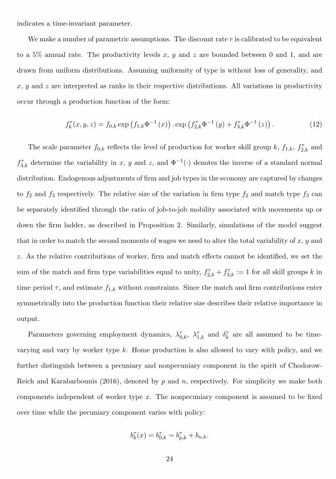
indicates a time-invariant parameter.

We make a number of parametric assumptions. The discount rate r is calibrated to be equivalent

to a 5% annual rate. The productivity levels x, y and z are bounded between 0 and 1, and are

drawn from uniform distributions. Assuming uniformity of type is without loss of generality, and

x, y and z are interpreted as ranks in their respective distributions. All variations in productivity

occur through a production function of the form:

f τk (x, y, z) = f0,k exp(f1,kΦ

−1 (x)). exp

(f τ2,kΦ

−1 (y) + f τ3,kΦ−1 (z)

). (12)

The scale parameter f0,k reflects the level of production for worker skill group k, f1,k, fτ2,k and

f τ3,k determine the variability in x, y and z, and Φ−1(·) denotes the inverse of a standard normal

distribution. Endogenous adjustments of firm and job types in the economy are captured by changes

to f2 and f3 respectively. The relative size of the variation in firm type f2 and match type f3 can

be separately identified through the ratio of job-to-job mobility associated with movements up or

down the firm ladder, as described in Proposition 2. Similarly, simulations of the model suggest

that in order to match the second moments of wages we need to alter the total variability of x, y and

z. As the relative contributions of worker, firm and match effects cannot be identified, we set the

sum of the match and firm type variabilities equal to unity, f τ2,k + f τ3,k := 1 for all skill groups k in

time period τ , and estimate f1,k without constraints. Since the match and firm contributions enter

symmetrically into the production function their relative size describes their relative importance in

output.

Parameters governing employment dynamics, λτ0,k, λτ1,k and δτk are all assumed to be time-

varying and vary by worker type k. Home production is also allowed to vary with policy, and we

further distinguish between a pecuniary and nonpecuniary component in the spirit of Chodorow-

Reich and Karabarbounis (2016), denoted by p and n, respectively. For simplicity we make both

components independent of worker type x. The nonpecuniary component is assumed to be fixed

over time while the pecuniary component varies with policy:

bτk(x) = bτ0,k = bτp,k + bn,k.

24

The pecuniary component of home production is calibrated prior to the estimation by fitting a

step function to the mean of income for the unemployed6, as shown in Appendix A.11. The aver-

age pecuniary value of home production is affected not just by the generosity of payments during

unemployment but also, amongst other things, by the relative number of long-term unemployed

who receive lower payments than the short-term unemployed both before and after the reforms, as

explained in Appendix A.1. In addition to the generosity of payments received during unemploy-

ment, this calibration of the flow benefit of unemployment thus also partly captures the prospects

of the unemployed.

We estimate a vector of exogenous parameters, which is θk ∈ Θ ∈ R20 for a skill group k and is

defined below. The vector arrows denote that the respective parameters change after every policy

wave and are thus four dimensional objects.

θk =(~λ0,k,

~λ1,k,~δk, bn,k, f0,k, f1,k,

~f2,k, βk

)

4.3 Identification

Identification of the model’s parameters motivates our choice of moments. While parameters are

co-dependent to some degree, each parameter is particularly relevant for certain series. Specifically,

the parameters to be estimated are the offer arrival rate for the unemployed λ0, the job arrival

rate for the employed λ1, the exogenous separation rate δ, the level of work production f0, the

variabilities in worker type f1, in firm type f2 and in match type f3, the non-pecuniary aspects of

home production home production bn, and the worker’s bargaining power β.

Employment dynamics are primarily governed by job offer arrival rates and separation rates.

While the breadth of matching sets and endogenous separations also matter, the rate at which

workers find jobs and lose them identify λ0, λ1 and δ. The degree of variation in worker and firm

type f1 and f2 are identified by the mean duration of unemployment of the newly employed and the

proportion of job-to-job transitions moving up the firm ladder. To understand why the duration of

unemployment determines the variation in worker type, consider the case where f1 = 0, all workers

6In order to be consistent with the estimation we take out a linear trend component that is extrapolated from

historic data.

25

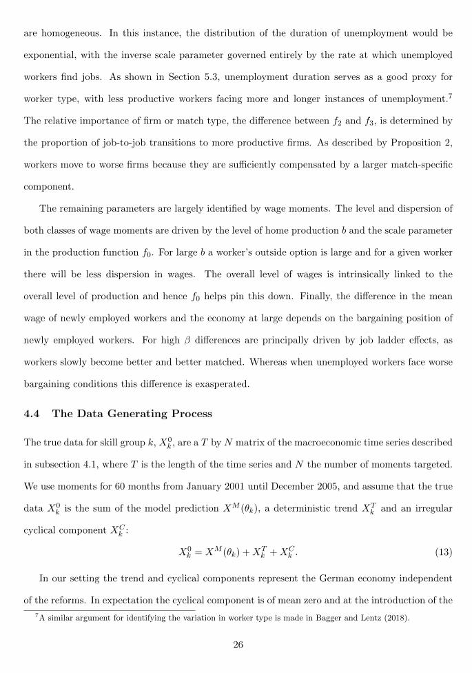
are homogeneous. In this instance, the distribution of the duration of unemployment would be

exponential, with the inverse scale parameter governed entirely by the rate at which unemployed

workers find jobs. As shown in Section 5.3, unemployment duration serves as a good proxy for

worker type, with less productive workers facing more and longer instances of unemployment.7

The relative importance of firm or match type, the difference between f2 and f3, is determined by

the proportion of job-to-job transitions to more productive firms. As described by Proposition 2,

workers move to worse firms because they are sufficiently compensated by a larger match-specific

component.

The remaining parameters are largely identified by wage moments. The level and dispersion of

both classes of wage moments are driven by the level of home production b and the scale parameter

in the production function f0. For large b a worker’s outside option is large and for a given worker

there will be less dispersion in wages. The overall level of wages is intrinsically linked to the

overall level of production and hence f0 helps pin this down. Finally, the difference in the mean

wage of newly employed workers and the economy at large depends on the bargaining position of

newly employed workers. For high β differences are principally driven by job ladder effects, as

workers slowly become better and better matched. Whereas when unemployed workers face worse

bargaining conditions this difference is exasperated.

4.4 The Data Generating Process

The true data for skill group k, X0k , are a T by N matrix of the macroeconomic time series described

in subsection 4.1, where T is the length of the time series and N the number of moments targeted.

We use moments for 60 months from January 2001 until December 2005, and assume that the true

data X0k is the sum of the model prediction XM (θk), a deterministic trend XT

k and an irregular

cyclical component XCk :

X0k = XM (θk) +XT

k +XCk . (13)

In our setting the trend and cyclical components represent the German economy independent

of the reforms. In expectation the cyclical component is of mean zero and at the introduction of the

7A similar argument for identifying the variation in worker type is made in Bagger and Lentz (2018).

26

first wave of reforms, we set the trend equal to zero. Given this normalization the effects of the Hartz

reforms can be uncovered from changes in XM (θk) after subtracting other changes that would have

happened in the absence of the reforms. The model and trend components are deterministic but

the cyclical component is random. The cyclical component XCk allows us to specify an analytical

likelihood function, as for any XM (θk) and XTk there exists an XC

k to rationalize the true data X0k .

The trend and cyclical components are fitted from January 1993 until February 2002. This

period corresponds to the first inclusion of a representative East German sample in the data up

to the formation of the Hartz Committee. The trend of each moment is assumed to be linear.

Results for non-linear trends with higher order polynomials are qualitatively similar. We assume

the cyclical component for skill group k to be drawn independently from a multivariate normal

distribution with mean zero and variance-covariance matrix Σk.

The likelihood function describes the likelihood of observing the innovative shocks required to

rationalize the observed data. For a Σk the vector of innovative shocks at time t is defined as a

function of the vector of structural parameters θk.

εt,k(θk) = x0t,k − xM

t (θk)− xTt,k

Since εt,k(θk) is distributed following a multivariate normal distribution with mean zero and

variance-covariance matrix Σk, we can write the likelihood function as

L(ε1,k(θk), ..., εt,k(θk)) =T∏

t=1

g(εt,k(θk)|Σk; εt−1,k(θk))

=(2π)−NT2 .|Σk|−

T2 . exp

{−1

2

T∑

t=1

εt,k(θ)′Σ−1k εt,k(θk)

}. (14)

T is the length of the time series, N is the number of series, g(·) is the probability density of a

multivariate normal distribution, and | · | represents the determinant. Instead of maximizing the

likelihood, we minimize its natural log.

To improve the fit of the moments and to increase the functionality of the estimation procedure,

we make two refinements. The likelihood function is highly nonlinear, which is partly due to

spikes in employment dynamics at the instance of policy implementation, and particularly in the

27

endogenous job destruction process. Endogenous job destructions occur at the announcement or

implementation of policy reform. The mass of matches that are no longer feasible depends on the

history of all other variables and can be large, so that they are only rationalized by improbably

large draws of ε. To smooth the likelihood function and to decrease the dimensionality of the

problem we remove the months of implementation from the criterion.8

5 Results

This section presents the parameter estimates and the fit of the targeted dynamics of the model.

We then simulate the model at steady-state before and after the reforms and evaluate the aggregate

impact of the policies and the relative importance of successive policy waves.

5.1 Parameter Estimates

The parameter estimates of the model are reported in Table 3, with asymptotic standard errors in

the parentheses below the point estimates. To ensure that the estimates represent global minima of

the log-likelihood function (14) we initiate our estimation with parallel runs of a Metropolis-Hastings

type algorithm, which is not as susceptible to stopping at local minima as a standard hill-climbing

algorithm. The numbered superscripts correspond to time separated by policy implementation.9

We first focus on the levels of the estimates, and discuss the evolution of the parameters in Section

5.3.

The monthly job offer arrival rates are larger than in most previous studies, which is due to the

frequency with which job offers are rejected. Back of the envelope calculations suggest for every

offer accepted by an unemployed worker between four and ten are rejected on average, depending

on the period and the skill group. The number of rejected jobs increases sharply with skill. While

larger than in much previous work, it is hard to verify whether the proportion of job offers leading to

matches is reasonable, as typically only accepted offers are observed in the data. That said, using

8We thank an anonymous referee for this suggestion.9Specifically, the numbers denote (1) before the first wave, (2) after the first but before the second wave, (3) after

the second but before the third wave, and (4) after the third and final wave.

28

Table 3: Parameter estimates

Low-skill Medium-skill High-skill

λ(1)0 λ

(2)0 λ

(3)0 λ

(4)0 λ

(1)0 λ

(2)0 λ

(3)0 λ

(4)0 λ

(1)0 λ

(2)0 λ

(3)0 λ

(4)0

0.372(0.0007)

0.352(0.0007)

0.332(0.0006)

0.328(0.0006)

0.895(0.0011)

0.918(0.0011)

0.935(0.0012)

0.915(0.0011)

1.04(0.0014)

0.997(0.0014)

0.946(0.0013)

0.711(0.0010)

λ(1)1 λ

(2)1 λ

(3)1 λ

(4)1 λ

(1)1 λ

(2)1 λ

(3)1 λ

(4)1 λ

(1)1 λ

(2)1 λ

(3)1 λ

(4)1

0.136(0.0003)

0.139(0.0003)

0.110(0.0002)

0.140(0.0003)

0.246(0.0003)

0.205(0.0003)

0.200(0.0005)

0.399(0.0003)

0.409(0.0006)

0.331(0.0004)

0.330(0.0004)

0.343(0.0005)

δ(1) δ(2) δ(3) δ(4) δ(1) δ(2) δ(3) δ(4) δ(1) δ(2) δ(3) δ(4)

0.0082(0.0000)

0.0099(0.0000)

0.0101(0.0000)

0.0104(0.0000)

0.0089(0.0000)

0.0101(0.0000)

0.0101(0.0000)

0.0090(0.0000)

0.0045(0.0000)

0.0048(0.0000)

0.0049(0.0000)

0.0047(0.0000)

f0 f1 β f0 f1 β f0 f1 β28.3

(0.0529)0.934(0.0017)

0.232(0.0004)

28.3(0.0351)

0.885(0.0011)

0.234(0.0003)

73.3(0.0995)

1.40(0.0019)

0.22(0.0003)

f(1)2 f

(2)2 f

(3)2 f

(4)2 f

(1)2 f

(2)2 f

(3)2 f

(4)2 f

(1)2 f

(2)2 f

(3)2 f

(4)2

0.387(0.0007)

0.417(0.0007)

0.461(0.0009)

0.527(0.0010)

0.639(0.0008)

0.641(0.0008)

0.639(0.0008)

0.640(0.0008)

0.747(0.0010)

0.723(0.0010)

0.798(0.0011)

0.794(0.0011)

b(1)0 b

(2)0 b

(3)0 b

(4)0 b

(1)0 b

(2)0 b

(3)0 b

(4)0 b

(1)0 b

(2)0 b

(3)0 b

(4)0

0.215(0.0340)

−0.154(0.0054)

−0.066(0.0054)

−0.144(0.0054)

0.570(0.0270)

−0.0970(0.0039)

−0.0592(0.0038)

0.0693(0.0038)

0.607(0.0439)

−1.00(0.0047)

−1.70(0.0047)

−2.53(0.0046)

Notes: All parameter estimates are reported to three significant figures. Asymptotic standard errors are presented

in the parenthesis and reported to four decimal places. The numbered superscripts in parentheses denote (1) before

the first wave, (2) after the first but before the second wave, (3) after the second but before the third wave, and (4)

after the third and final wave.

a unique dataset on job seekers, Faberman et al. (2017) find that approximately one-seventh of

employer contacts with unemployed workers lead to a job.10 This proportion, from a U.S. context,

is broadly in line with our value for Germany. For all three skill groups, an unemployed worker

extracts approximately a quarter of the surplus from the firm. While this value is somewhat smaller

than is often estimated in the literature, this bargaining power is compensated by later negotiations

triggered by outside offers, where the worker may be able to extract more rents from the firm.

The productivity parameters indicate the relative importance of worker, firm and match type in

production. Worker type appears the most important in determining total output, governed by f1.

For medium- and high-skill workers firm type is more consequential than match type and f2 > 0.5.

But for the low-skilled the job-specific component is more important than the firm type.

10This number is derived from moments reported in Faberman et al. (2017), by calculating (mean offers in a month

× proportion of all offers accepted)/mean contacts received in a month = (0.373 × 0.483)/1.261 ≈ 1/7.

29

5.2 The Fit

In this section we present the fit of the moments targeted in estimation. The simulated series are

displayed in Figures 4, 5 and 6 for low-, medium- and high-skilled workers respectively. The solid

black line represents the data and the blue line denotes the simulation. The shaded blue area is the

95% confidence interval obtained by repeated redrawing of the series of shocks. Overall, the model

matches the level and dynamics of the targeted moments, with a number of deviations between the

simulations of the estimated moments and the data discussed here.

Firstly, for low- and medium-skilled workers, the moment that captures the proportion of job

switchers moving to a more productive firm does not match the data closely in terms of the level

and dynamics, which is a consequence of imposing the identity f τ2,k + f τ3,k := 1 on the model. As

long as the the overall job-to-job transition rate is matched well, the lack of a better fit for this

moment has a negligible effect on our main findings. As a result, however, findings regarding the

impact of the Hartz reforms on the relative importance of firms and jobs for good matches are

not fully reliable. Further, the job finding rate of the unemployed exhibits an upturn at the end

of the sample window in 2005 for all three skill groups that is present in the data and not in our

simulations. We underestimate the job finding rate for this period across each skill group because

the final discontinuity in our model is in January of 2005.

With respect to the wage moments, recall the model only matches these moments pre-reform,

in order not to impose how wages are re-negotiated after policy changes. The model does not

jointly match the wage distribution of the newly employed and the distribution of wages overall,

and the model over-predicts the ratio of the overall mean wage in the economy relative to the mean

wage of the newly employed across the three skill groups.11 Although the levels are not matched

precisely, the trend across each skill is well-fitted, and the wage effects of the reforms can therefore

be credibly inferred from our model.

11Due to the trade-off between the mean of wages and their standard deviations, we cannot simply reconcile the

relative mean wage predictions by decreasing worker bargaining power β. If we reduce β the measured dispersion in

overall wages increases, which is a moment that is already over-estimated. A lower β drives up the variance of log

wages by increasing the mass at the left tail of the distribution, as the lowest earners tend to those hired straight

from unemployment. This effect has a larger impact on the left rather than right tail as it is not subject to censoring.

30

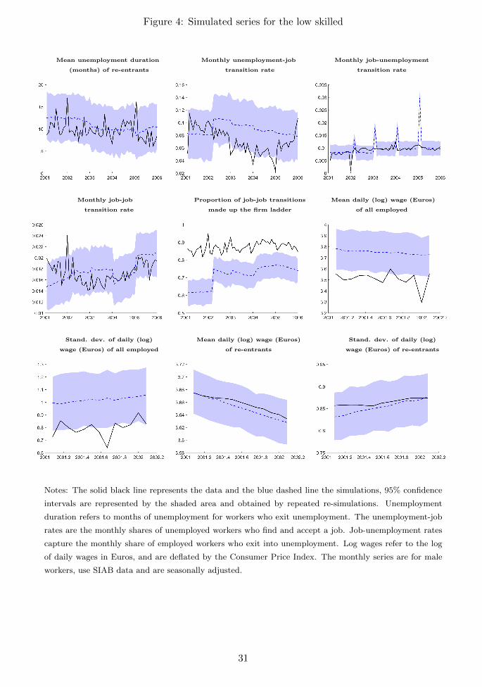
Figure 4: Simulated series for the low skilled

Mean unemployment duration Monthly unemployment-job Monthly job-unemployment

(months) of re-entrants transition rate transition rate

Monthly job-job Proportion of job-job transitions Mean daily (log) wage (Euros)

transition rate made up the firm ladder of all employed

Stand. dev. of daily (log) Mean daily (log) wage (Euros) Stand. dev. of daily (log)

wage (Euros) of all employed of re-entrants wage (Euros) of re-entrants

Notes: The solid black line represents the data and the blue dashed line the simulations, 95% confidence

intervals are represented by the shaded area and obtained by repeated re-simulations. Unemployment

duration refers to months of unemployment for workers who exit unemployment. The unemployment-job

rates are the monthly shares of unemployed workers who find and accept a job. Job-unemployment rates

capture the monthly share of employed workers who exit into unemployment. Log wages refer to the log

of daily wages in Euros, and are deflated by the Consumer Price Index. The monthly series are for male

workers, use SIAB data and are seasonally adjusted.

31

Figure 5: Simulated series for the medium skilled














32

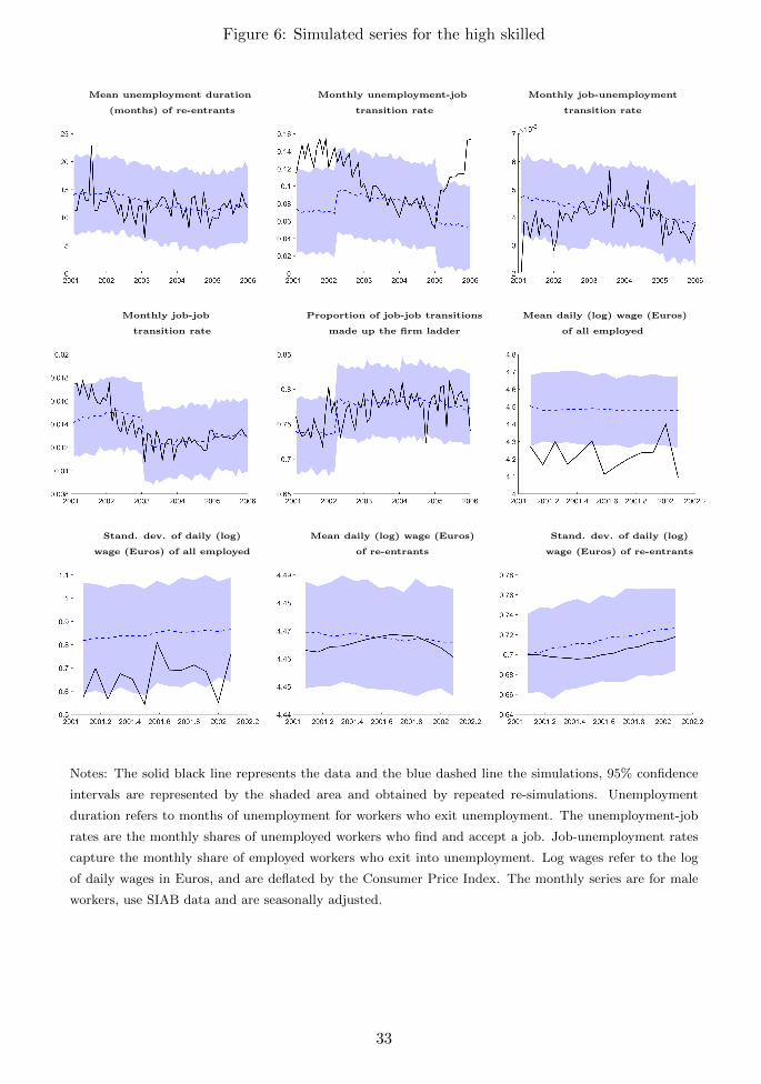
Figure 6: Simulated series for the high skilled














33

While in the estimation we target only the mean and the standard deviation of wages, in

Appendix A.12 we present kernel plots of simulated and real wage data for each skill group. Since

the targeted moments are subject to top-coding we also present the distribution of wages our model

predicts, absent of censoring.

5.3 Simulations

The persistence of employment and wages makes inference about the long-run impact of the Hartz

reforms difficult. Using our structural framework we can determine the long-run effect on employ-

ment by computing the steady-state wage distribution, evaluated at the parameter estimates pre-

and post-reform.

5.3.1 Aggregate Outcomes

To investigate the long-run impact of the three reform waves jointly, we compare employment and

wages in two steady-states, one for the initial values of the structural parameters and the other one

for the structural parameter values after the final reform wave implementation. Table 4 presents

the impact directly attributable to the Hartz reforms before and after the policies are implemented.

The final column is weighted according to the relative sizes of the three skill groups given in Table

2.

Table 4: Combined impact of the Hartz reforms

Low skill Medium skill High skill Aggregate

Employment rate -0.95 +0.05 -0.68 -0.16

percentage point change

Wage -10.69 -3.66 -2.90 -4.12

percentage change

Our key finding is that the Hartz reforms decreased employment by 0.16 percentage points, and

this negligible fall in employment came with a fall in wages of 4.12%. By contrast, the objective of

policymakers was to achieve a significant decrease in unemployment. Inspection of the first three

columns in Table 4 highlights the distributional impact of the policy, with the low skilled bearing

34

the brunt of the wage costs. Mean wages for workers without formal qualifications fell by 10.69%.

This group also suffered the largest declines in employment, with the employment rate dropping

by two thirds of a percentage point. While all groups suffered as a consequence of the reforms, the

low skilled were hit hardest. The slight fall in low-skilled employment seems to contradict the rise

in the job finding rate exhibited in Figure 4, but the increase in the job finding rate is a comparison

of two steady-states while the fall in low-skilled employment in Figure 4 displays off steady-state

dynamics. In this setting the job finding rate is likely to be higher out of steady-state as the labor

market is still adjusting.

Since our analysis compares two steady-states, changes in employment are governed by changes

in the rate at which workers find and lose jobs. For all but the highest-skilled workers, the Hartz

reforms led to a rise in both job finding and separation rates, so that the ex-ante employment effect

is ambiguous. It turns out that aggregated, these two effects almost perfectly offset one another in

determining the overall impact on employment. Despite minimal changes to the overall employment

rate, the experience of a typical unemployed worker is likely to change considerably as a consequence

of the reforms. Workers receive less remuneration while in unemployment, but can on average,

expect a shorter duration of their spell. Previously, the low, medium and high skilled on average

expected an unemployment duration of 12.0, 9.6 and 13.6 months, respectively. In the aftermath of

the reforms, however, expected unemployment duration shortened to 10.3 months for the low skilled

and to 9.4 months for the medium skilled. Only the highest-skilled workers experience a rise in

expected unemployment duration, with an increase to 14.8 months. Even though our overall results

show little aggregate employment impact, these changes in unemployment duration highlight that

the reforms were consequential for changing the flexibility of the labor market.

5.3.2 Individual Hartz Reforms

We further investigate the impact of each reform separately, as well as of pairs of reform waves.

The effects of the first wave and the first and second waves jointly can be uncovered without any

further parametric assumptions. Since we estimate the vector of structural parameters pre- and

post-reform in both instances, it is straightforward to simulate the steady-state economy imposing

35

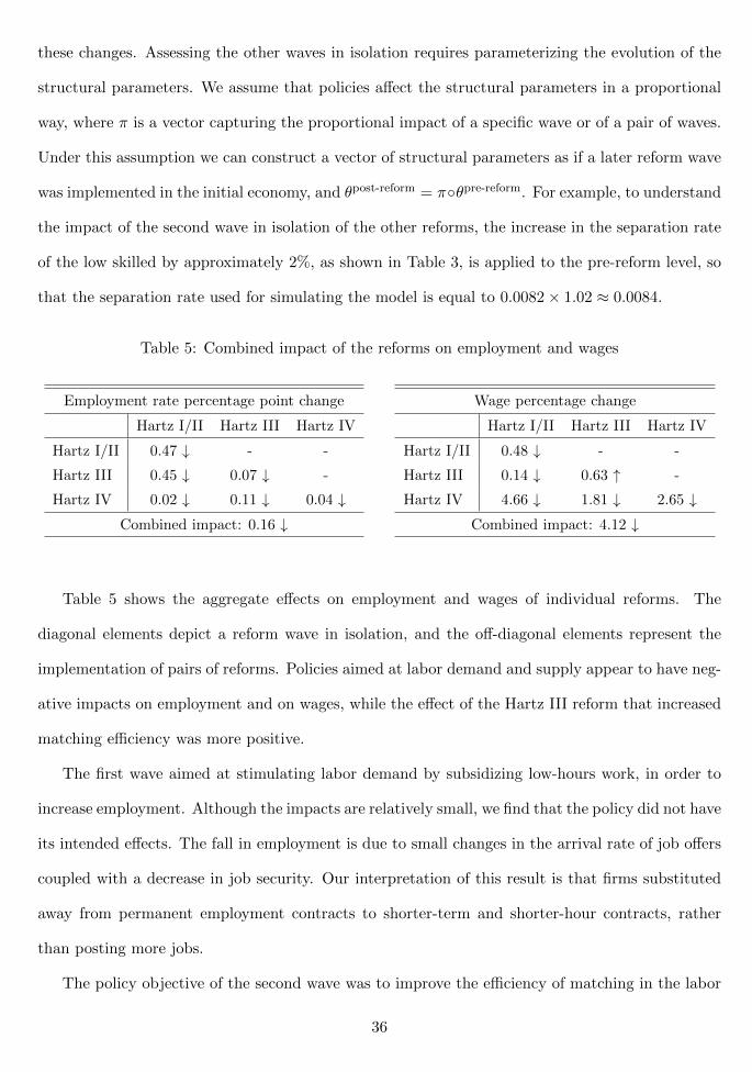
these changes. Assessing the other waves in isolation requires parameterizing the evolution of the

structural parameters. We assume that policies affect the structural parameters in a proportional

way, where π is a vector capturing the proportional impact of a specific wave or of a pair of waves.

Under this assumption we can construct a vector of structural parameters as if a later reform wave

was implemented in the initial economy, and θpost-reform = π◦θpre-reform. For example, to understand

the impact of the second wave in isolation of the other reforms, the increase in the separation rate

of the low skilled by approximately 2%, as shown in Table 3, is applied to the pre-reform level, so

that the separation rate used for simulating the model is equal to 0.0082× 1.02 ≈ 0.0084.

Table 5: Combined impact of the reforms on employment and wages

Employment rate percentage point change

Hartz I/II Hartz III Hartz IV

Hartz I/II 0.47 ↓ - -

Hartz III 0.45 ↓ 0.07 ↓ -

Hartz IV 0.02 ↓ 0.11 ↓ 0.04 ↓Combined impact: 0.16 ↓

Wage percentage change

Hartz I/II Hartz III Hartz IV

Hartz I/II 0.48 ↓ - -

Hartz III 0.14 ↓ 0.63 ↑ -

Hartz IV 4.66 ↓ 1.81 ↓ 2.65 ↓Combined impact: 4.12 ↓

Table 5 shows the aggregate effects on employment and wages of individual reforms. The

diagonal elements depict a reform wave in isolation, and the off-diagonal elements represent the

implementation of pairs of reforms. Policies aimed at labor demand and supply appear to have neg-

ative impacts on employment and on wages, while the effect of the Hartz III reform that increased

matching efficiency was more positive.

The first wave aimed at stimulating labor demand by subsidizing low-hours work, in order to

increase employment. Although the impacts are relatively small, we find that the policy did not have

its intended effects. The fall in employment is due to small changes in the arrival rate of job offers

coupled with a decrease in job security. Our interpretation of this result is that firms substituted

away from permanent employment contracts to shorter-term and shorter-hour contracts, rather

than posting more jobs.

The policy objective of the second wave was to improve the efficiency of matching in the labor

36

market. We find no discernible impact of the Hartz III reform on employment, with the arrival rate

of job offers falling for the low and high skilled and rising for the medium skilled. The policy lifts

the flow value associated with unemployment, which could potentially happen if the job seeking

assistance provided freed up time for the unemployed. This rise in b lifts wages for two reasons: the

unemployed are able to choose only better suited matches, and the outside option of the unemployed

in wage bargaining with a given firm increases.

The final wave has the most pronounced effects on wages. These effects are driven by a reduction

in the flow value of unemployment that is due to the reduction in the generosity of unemployment

benefit. In isolation, the reduction in unemployment benefit, would generate larger wage effects

than the 2.6% reduction that our model predicts. However, following the reform there is also an

increase in the rate at which employed workers received job offers. This phenomenon occurs for all

three skill groups. Consequently, the fall in wages are partially offset because of steeper job ladder

effects. The employment effects however, are negligible. Although the response in labor demand

is strong it has almost no effect on the level of employment, as the beneficiaries of this response

are employed, rather than unemployed workers. Inspection of Table 3 shows that while λ1 grew

considerably for all groups, and by contrast λ0 fell or grew by small amounts.

6 Conclusion

This paper evaluates the comprehensive Hartz reforms on the German labor market. We construct

and estimate a model of the labor market with forward-looking agents, search frictions and hetero-

geneity of workers by education level. These labor market features are critical for understanding

the impact of labor market policy changes in many contexts, where detailed worker-firm data are

available.

In our setting, the Hartz labor market reform laws are treated as shocks to the structural

parameters, which are fully anticipated by forward-looking agents. To assess the effects of the

German Hartz reforms the model is estimated by maximum likelihood estimation with matched

worker-firm data. Identification exploits the off steady-state dynamics of the model. The results of

37

our evaluation show that the Hartz reforms had a negligible impact on employment and at the same

time reduced wages. The primary driver of this reduction in wages is the final wave of reforms,

which reduced the generosity of unemployment benefits in particular for the long-term unemployed.

Our paper shows that a comprehensive approach to evaluating labor market policy changes

provides insights that are not easily obtained in reduced-form assessments of particular reform

aspects, or with calibrated macro models. The evaluation approach we propose makes use of

detailed administrative data on workers and firms, which have recently become available for an

increasing number of countries. In this framework, detailed data enable a careful assessment of the

impacts of complex and multifaceted policy.

38

References

Attanasio, O. P., C. Meghir and A. Santiago, “Education Choices in Mexico: Using a

Structural Model and a Randomized Experiment to Evaluate PROGRESA,” Review of Economic

Studies 79 (2012), 37–66.

Bagger, J. and R. Lentz, “An Empirical Model of Wage Dispersion with Sorting,” forthcoming,

Review of Economic Studies (2018).

Bentolila, S., P. Cahuc, J. J. Dolado and T. Le Barbanchon, “Two-Tier Labour Markets

in the Great Recession: France Versus Spain,” Economic Journal 122 (2012), 155–187.

Blundell, R. and A. Shephard, “Employment, Hours of Work and the Optimal Taxation of

Low Income Families,” Review of Economic Studies 79 (2012), 481–510.

Bradley, J., F. Postel-Vinay and H. Turon, “Public Sector Wage Policy and Labor Market

Equilibrium: A Structural Model,” Journal of the European Economic Association 15 (2017),

1214–1257.

Bundesagentur fur Arbeit, “Der Ubergang von der Arbeitslosen- und Sozialhilfe zur Grund-

sicherung fur Arbeitssuchende,” Special Report (2005).

Cahuc, P., F. Postel-Vinay and J.-M. Robin, “Wage Bargaining with On-the-Job Search:

Theory and Evidence,” Econometrica 74 (2006), 323–364.

Card, D., J. Heining and P. Kline, “Workplace Heterogeneity and the Rise of West German

Wage Inequality,” Quarterly Journal of Economics 128 (2013), 967–1015.

Chodorow-Reich, G. and L. Karabarbounis, “The Cyclicality of the Opportunity Cost of

Employment,” Journal of Political Economy 124 (2016), 1563–1618.

Dey, M. and C. Flinn, “An Equilibrium Model of Health Insurance Provision and Wage Deter-

mination,” Econometrica 73 (2005), 571–627.

39

Dustmann, C., B. Fitzenberger, U. Schonberg and A. Spitz-Oener, “From Sick Man of

Europe to Economic Superstar: Germany’s Resurgent Economy,” Journal of Economic Perspec-

tives 28 (2014), 167–188.

Ebbinghaus, B. and W. Eichhorst, “Employment Regulation and Labor Market Policy in

Germany, 1991-2005,” IZA Discussion Paper No. 2505 (2006).

Faberman, J., A. Mueller, A. Sahin and G. Topa, “Job Search Behavior among the Employed

and Non-Employed,” IZA Discussion Paper No. 10960 (2017).

Fahr, R. and U. Sunde, “Did the Hartz Reforms Speed-Up the Matching Process? A Macro-

Evaluation Using Empirical Matching Functions,” German Economic Review 10 (2009), 284–316.

Fitzenberger, B., A. Osikominu and R. Volter, “Imputation Rules to Improve the Education

Variable in the IAB Employment Subsample,” Schmollers Jahrbuch: Journal of Applied Social

Science Studies / Zeitschrift fur Wirtschafts- und Sozialwissenschaften 126 (2006), 405–436.

Galassi, G., “Labor Demand Response to Labor Supply Incentives: Evidence from the German

Mini-Job Reform,” mimeo (2017).

Hertweck, M. S. and O. Sigrist, “The Aggregate Effects of the Hartz Reforms in Germany,”

University of Basel Working Papers 2013/01 (2013).

Jacobi, L. and J. Kluve, “Before and After the Hartz Reforms: The Performance of Active

Labour Market Policy in Germany,” Zeitschrift fur ArbeitsmarktForschung 40 (2007), 45–65.

Keane, M. and R. Moffitt, “A Structural Model of Multiple Welfare Program Participation

and Labor Supply,” International Economic Review 39 (1998), 553–589.

Klinger, S. and T. Rothe, “The Impact of Labour Market Reforms and Economic Performance

on the Matching of the Short-term and the Long-term Unemployed,” Scottish Journal of Political

Economy 59 (2012), 90–114.

40

Koch, S. and U. Walwei, “Hartz IV: Neue Perspektiven fur Langzeitarbeitslose?,” Aus Politik

und Zeitgeschichte 16/2005 (2005), 10–17.

Krause, M. U. and H. Uhlig, “Transitions in the German Labor Market: Structure and Crisis,”

Journal of Monetary Economics 59 (2012), 64–79.

Krebs, T. and M. Scheffel, “Macroeconomic Evaluation of Labor Market Reform in Germany,”

IMF Economic Review 61 (2013), 664–701.

Launov, A. and K. Walde, “Estimating Incentive and Welfare Effects of Nonstationary Unem-

ployment Benefits,” International Economic Review 54 (2013), 1159–1198.

———, “The Employment Effect of Reforming a Public Employment Agency,” European Economic

Review 84 (2016), 140–164.

Lise, J. and J.-M. Robin, “The Macrodynamics of Sorting between Workers and Firms,” Amer-

ican Economic Review 107 (2017), 1104–35.

Murtin, F. and J.-M. Robin, “Labor Market Reforms and Unemployment Dynamics,” Labour

Economics 50 (2018), 3–19.

Postel-Vinay, F. and J.-M. Robin, “Equilibrium Wage Dispersion with Worker and Employer

Heterogeneity,” Econometrica 70 (2002), 2295–2350.

Postel-Vinay, F. and H. Turon, “On-the-job Search, Productivity Shocks, and the Individual

Earnings Process,” International Economic Review 51 (2010), 599–629.

Price, B., “The Duration and Wage Effects of Long-Term Unemployment Benefits: Evidence from

Germany’s Hartz IV Reform,” mimeo (2018).

Rothe, T. and K. Walde, “Where Did All the Unemployed Go? Non-standard Work in Germany

after the Hartz Reforms,” mimeo (2017).

Shephard, A., “Equilibrium Search and Tax Credit Reform,” International Economic Review 58

(2017), 1047–1088.

41

Tazhitdinova, A., “Does the Magnitude of Tax Incentives Matter? Labor Supply and Demand

Responses to an Unusually Large Tax Break,” mimeo (2018).

Weise, F.-J., “Der Umbau der Bundesanstalt/Bundesagentur fur Arbeit zum modernen Dien-

stleister,” Vierteljahrshefte zur Wirtschaftsforschung 80 (2011), 67–78.

42

A Appendix

A.1 The Hartz Reforms

The Hartz I and II laws came into effect on January 1st 2003. Hartz I facilitated temporary

employment, and introduced new training subsidies. The reform simplified and extended case-based

exemptions from relatively restrictive employment regulations (Jacobi and Kluve, 2007). Vouchers

for career development training of the unemployed were introduced by the Federal Employment

Agency to support measures with a maximum duration of three months. The reform also created

personnel service agencies, which serve as temporary work agencies to complement the existing local

employment agencies in finding job placements for unemployed workers. Hartz II provided further

regulation of marginal employment by increasing tax threshold for so-called mini- and midi-jobs, and

sponsored business startups by the unemployed. Mini-jobs allow exemption of worker contributions

to income tax and social security and lifted the threshold for such marginal tax-exempt employment

from a monthly income of 325 to 400 Euros. Midi-jobs incur reduced social security contributions

on a sliding scale for earnings up to 800 Euros per month. The definition of marginal employment

was also extended to employees working more than 15 hours per week. Hartz II further introduced

startup subsidies for the unemployed under the name Ich-AG (i.e. Me-Company), which resulted

in 270,000 such startups receiving subsidies from the Federal Employment Agency until the end of

2004. Further details about the reform elements and the number of workers affected are provided

in Ebbinghaus and Eichhorst (2006).

The third reform law, Hartz III, was implemented from January 1st 2004 on, and restructured

the Federal Employment Agency. The placement and job search support the employment admin-

istration and the management of its 90,000 employees was reorganized, so that the employment

agency would become a modern client-oriented service provider. Weise (2011) discusses the reor-

ganization of the Federal Employment Agency in greater detail.

Hartz IV came into effect on January 1st 2005 and significantly changed the structure and gen-

erosity of payments received during unemployment, with an aim to increase incentives to work.

Hartz IV combined parts of unemployment assistance with social assistance payments for the long-

43

term unemployed, and introduced sanctions to promote more active job search. In practice, the

effect of the change on the generosity of long-term unemployment payments is determined by worker

circumstances with post-reform receipts depending, for example, on the income of the partner and

the number of children. Additional allowances may be available for accommodation and heating.

Before Hartz IV, three types of payments existed for unemployed workers: unemployment insur-

ance payments (Arbeitslosengeld) for the short-term unemployed, and means-tested unemployment

assistance (Arbeitslosenhilfe) and social assistance for the long-term unemployed. The Hartz IV

reform did not change short-term benefits, which imply that eligible workers receive 60% of their

previous net wage in the case of unemployment, with a maximum duration of 32 months, depend-

ing on age and months worked previous to the unemployment spell. For short-term unemployed

workers with dependent children the replacement rate is 67%. After exhausting short-term benefits,

workers were eligible to time-unlimited unemployment assistance payments at a replacement rate

of 53% of previous net wages, and of 57% if they had dependent children. Hartz IV combined un-

employment assistance and social assistance for the long-term unemployed into a flat-rate payment

that is not indexed to previous wages, and that is now administered by the Federal Employment

Agency. This change decreased payments to many who previously received long-term unemploy-

ment assistance. Price (2018) provides a detailed overview of the eligibility rules and changes for

income replacement and support during unemployment. If acceptable job offers were declined, un-

employed workers could incur sanctions in the form of reduced benefits. Benefit payments became

more contingent on means testing, and the definition of acceptable job offers was widened. After

Hartz IV, unemployed workers were also required to take low-paid jobs including mini-jobs and

jobs that did not correspond to the level of a worker’s training or his previous job. In addition to

the Hartz IV law, reductions to unemployment benefit durations were announced in January 2005.

These changes applied to unemployment spells starting from February 2006 onward, so that the

first duration cuts took effect in 2007.

44

A.2 Wage Re-Negotiation: After a Policy Shock

Perhaps the simplest way to model wage re-negotiation would be to assume wages are fully flexible

and can be re-negotiated after the state of the world changes through policy shocks. In this hy-

pothetical scenario wages are re-negotiated assuming the worker has the same firm-match outside

option (y′, z′). The worker can only use this outside option as a bargaining tool with his cur-

rent employer, and we do not consider the possibility of changing employers. This re-negotiation

mechanism ensures tractability. After a shock, a match either dissolves and the worker returns to

unemployment, or wages are re-negotiated.

The match separates: The match dissolves if the participation (positive surplus) con-

straint no longer holds. The set of time-varying parameters θt′ immediately after a shock, for

which a (y, z) match with a worker of productivity x is endogenously destroyed, is given by

N0,t′(x, y, z) ≡ {θt′ |St′(x, y, z) < 0}.

If a worker’s outside option is unemployment, the outcome of the wage re-negotiation is trivial.

Before the shock a worker of type x in a match (y, z) earned a wage φ0,t(x, y, z). After a shock, as

long as the match is not separated, θt′ /∈ N0,t′(x, y, z), the worker’s new wage is given by φ0,t′(x, y, z).

These wages are determined as the solution to the equality given by equation (2).

If the same worker in the same match with an outside offer (y′, z′) and currently earning w :=

φ1,t(x, y, z, y′, z′), however, is hit by a shock, his new wage is re-negotiated in one of three ways.

In each case we denote the new wage as w′, which can be a function of a worker’s type (x), his job

type (y, z) and his best outside option (y′, z′).

Use the same outside offer: The worker’s new wage is re-negotiated using the same

firm-match threat point if θt′ is such that

N1,t′(x, y, z, y′, z′) ≡ {θt′ |St′(x, y, z) ≥ St′(x, y′, z′) ≥ βt′St′(x, y, z) ≥ 0}.

In this scenario the match remains incentive compatible. The worker uses the same threat

45

point when bargaining with his incumbent firm, and the new wage is given by

w′ = φ1,t′(x, y, z, y′, z′).

Use unemployment as outside offer:

N2,t′(x, y, z, y′, z′) ≡ {θt′ |βSt′(x, y, z) > St′(x, y

′, z′) ≥ 0}

Given the above, a worker gains a greater share of the surplus using unemployment as a

threat point as opposed to his previous best outside option. In the re-negotiation procedure

he bargains with unemployment as his outside option and his new wage is given by

w′ = φ0,t′(x, y, z).

The worker takes all the surplus:

N3,t′(x, y, z, y′, z′) ≡ {θt′ |St′(x, y′, z′) > St′(x, y, z) ≥ 0}

Finally, it could be that after realization of the new parameter set the outside option of the

worker generates a larger surplus than continued employment with his current firm. In our

setting, a worker cannot move to previous job offers, as in such a case a change in policy

would increase job mobility by construction. In this case we assume the worker has all the

bargaining power and is able to extract the entire surplus. His new wage is given by

w′ = φ1,t′(x, y, z, y, z).

A.3 Value Functions

The present discounted value of an unemployed worker of productivity x is equal to bt(x), the flow

utility of unemployment, the option value of employment and the associated change if a policy is

implemented:

rUt(x) = bt(x)+λ0,t

∫ ∫

y′,z′∈M0,t(x)[Wt(φ0,t(x, y

′, z′), x, y′, z′)− Ut(x)]υ(y′)γ(z′)dy′dz′

+ηt[Ut′(x)− Ut(x)]

46

Using the identity given by equation (2), the above simplifies to:

rUt(x) = bt(x) + βλ0,t

∫ ∫

y′,z′∈M0,t(x)St(x, y

′, z′)υ(y′)γ(z′)dy′dz′ + ηt[Ut′(x)− Ut(x)]

The value function for an employed worker of productivity x in a firm of productivity y with a

match-specific draw z earning a wage w at time t, is more cumbersome:

rWt(w, x, y, z) = w + δt[Ut(x)−Wt(w, x, y, z)]

+ λ1,t

∫ ∫

y′,z′∈M10,t(x,y,z)[Wt(φ0,t(x, y

′, z′), x, y′, z′)−Wt(w, x, y, z)]υ(y′)γ(z′)dy′dz′

+ λ1,t

∫ ∫


′, z′, y, z), x, y′, z′)−Wt(w, x, y, z)]υ(y′)γ(z′)dy′dz′

+ λ1,t

∫ ∫

y′,z′∈M2,t(w,x,y,z)[Wt(φ1,t(x, y, z, y

′, z′), x, y, z)−Wt(w, x, y, z)]υ(y′)γ(z′)dy′dz′

+ ηt

[1{St′(x, y, z) < 0}Ut′(x) + 1{St′(x, y, z) ≥ 0}Wt′(w

r, x, y, z)−Wt(w, x, y, z)]

The four option values in the above expression are unemployment risk, finding a much better job

and using unemployment as a threat point, finding a better job and using the current employer

as a threat point, and promotion within one’s current employer. Unemployment occurs if a match

is exogenously dissolved, which happens at the Poisson rate δt. After a worker meets a new firm,

depending on the draw of y′ and z′, the worker may move if the pair falls in the setM1,t(x, y, z). If

the new job is sufficiently better than the current one (y′, z′) ∈ M10,t(x, y, z) then unemployment

is used as a threat point. If the draw is a small improvement, and (y′, z′) ∈M11,t(x, y, z), then the

worker uses his current employer as a threat point in Bertand competition. Finally, a worker gets a

within firm promotion if his new offer (y′, z′) ∈M2,t(w, x, y, z). All these sets are formally defined

in Section 3.3.

In addition to the option value of employment there is a possibility that labor market reforms

change the employment value. These reforms occur at a Poisson rate ηt and their implications

depend on the way in which matched agents re-negotiate their employment contract. As discussed

in the body of the paper we wish to remain agnostic and simply say the re-negotiated wage is wr.

In the interest of brevity we label this wage as simple wr but this could be written as a function of

any of the variables in the model. Finally, although we don’t specify the exact wage re-negotiation

47

mechanism we do stipulate that if a worker-firm partnership now generates negative surplus we

assume they separate by mutual consent.

If one subtracts the value of unemployment from the value of employment as defined previously

and applies the identity given by equation (3), then the surplus generated for a worker earning a

wage w of productivity x in a firm of productivity y with match-specific productivity z at time t is

derived as the following expression. The worker surplus is defined as the value of employment net

of the worker’s outside option, unemployment.

(r + δt + ηt)[Wt(w, x, y, z)− Ut(x)] = w − bt(x)

+ λ1,t

∫ ∫

y′,z′∈M10,t(x,y,z)[βSt(x, y

′, z′) + Ut(x)−Wt(w, x, y, z)]υ(y′)γ(z′)dy′dz′

+ λ1,t

∫ ∫

y′,z′∈M11,t(x,y,z)[St(x, y, z) + Ut(x)−Wt(w, x, y, z)]υ(y′)γ(z′)dy′dz′

+ λ1,t

∫ ∫

y′,z′∈M2,t(w,x,y,z)[St(x, y

′, z′) + Ut(x)−Wt(w, x, y, z)]υ(y′)γ(z′)dy′dz′

− βλ0,t∫ ∫


′, z′)υ(y′)γ(z′)dy′dz′

+ ηt1{St′(x, y, z) ≥ 0} [Wt′(wr, x, y, z)− Ut′(x)]

Turning to the firm, the value for a firm of productivity y, hiring a worker of productivity x at a

wage rate w with a match-specific productivity of z at time t is given by the function Πt(w, x, y, z).

rΠt(w, x, y, z) = ft(x, y, z)− w + δt[0−Πt(w, x, y, z)]

+ λ1,t

∫ ∫

y′,z′∈M1,t(x,y,z)[0−Πt(w, x, y, z)]υ(y′)γ(z′)dy′dz′

+ λ1,t

∫ ∫

y′,z′∈M2,t(w,x,y,z)[Πt(φ1,t(x, y, z, y

′, z′), x, y, z)−Πt(w, x, y, z)]υ(y′)γ(z′)dy′dz′

+ ηt1{St′(x, y, z) < 0}[0−Πt(w, x, y, z)] + ηt1{St′(x, y, z) ≥ 0}[Πt′(wr, x, y, z)−Πt(w, x, y, z)]

The value function for the firm is analogous to that of the worker with a few exceptions. The

flow value of the match is the total output produced ft(x, y, z) net of the wage paid w, the outside

option of the firm is zero and not unemployment, and the firm does not care about the terms of

the worker’s next job, just if the worker leaves. Summing the above two expressions and applying

the identity in equation (1) yields the total surplus generated by a match of a worker with ability

48

x and a firm of productivity y with a match-specific productivity of z at time t.

(r + δt + ηt)St(w, x, y, z) = ft(x, y, z)− bt(x)− βλ0,t∫ ∫



+ λ1,t

∫ ∫

y′,z′∈M10,t(x,y,z)

[βSt(x, y

′, z′)− St(x, y, z)]υ(y′)γ(z′)dy′dz′

+ ηt1{St′(x, y, z) ≥ 0} [Wt′(wr, x, y, z)− Ut′(x) + Πt′(w

r, x, y, z)]

Transferable utility means the final term is the surplus in period t′. Inspection of the sets

M0,t(x) and M10,t(x), reveals the surplus equation can be expressed in a simpler way. Following

the notation of Lise and Robin (2017) we denote A+ := max{A, 0}. The surplus is independent of

the wage rate, which validates the assumption of transferable utility.

(r + δt+ηt)St(x, y, z) = ft(x, y, z)− bt(x)− βλ0,t∫ ∫


+ λ1,t

∫ ∫ [βSt(x, y

′, z′)− St(x, y, z)]+υ(y′)γ(z′)dy′dz′ + ηtSt′(x, y, z)

+

A.4 Proofs of Lemma 1, Proposition 1 and Lemma 2

A.4.1 Lemma 1

Given the regularity condition imposed on f that limz→z ft(x, y, z) = ∞, and taking the limit of

the right hand side of equation (4) implies:12

limz→z

((r + δt + ηt)St(x, y, z)) =∞+ Ct(x) +Dt(x, y) + Et(x, y)

where Ct(x) = −bt(x)− βλ0,t∫ ∫


and Dt(x, y) = λ1,t limz→z

(∫ y

y

∫ z

z

{βSt(x, y

′, z′)− St(x, y, z)}+

γ(z′)dz′υ(y′)dy′)

and Et(x, y) = ηt limz→z

(ηtSt′(x, y, z)

+)

Ct(x) is a constant for given x, and thus the limit properties of St(x, y, z) are independent of

this term. Further, it is assumed that St : (x, x)× (y, y)× (z, z)→ R.

12The term Et(x, y) is indexed by t, as by definition t′ is the period that arrives immediately after t.

49

(i) Assume limz→z St(x, y, z) is equal to a finite number. Then Dt(x, y) would equal a finite

number. Et(x, y) = ∞ for limz→z St′(x, y, z) = ∞ and Et(x, y) is equal to a finite num-

ber in all other situations. Thus, irrespective of the feasible value that Et(x, y) takes,

limz→z St(x, y, z) =∞, which is inconsistent with our assumption.

(ii) Assume limz→z St(x, y, z) = −∞. Then Dt(x, y) =∞ and Et(x, y) =∞ for

limz→z St′(x, y, z) =∞ and Et(x, y) is equal to a finite number in all other situations. Again,

limz→z St(x, y, z) =∞, which is inconsistent with our assumption.

(iii) Finally, assume limz→z St(x, y, z) =∞. ThenDt(x, y) would equal a finite number. Et(x, y) =

∞ for limz→z St′(x, y, z) =∞ and Et(x, y) is equal to a finite number in all other situations.

Thus, irrespective of the feasible value that Et(x, y) takes, limz→z St(x, y, z) = ∞, which is

consistent with our assumption. Q.E.D.

A.4.2 Proposition 1

To prove Proposition 1, it is enough to show that for any (x, y) there is a z such that St(x, y, z) ≥ 0.

For fixed x and y, the fact that St(x, y, z) is positive translates to the condition that:

ft(x, y, z) +N1(z) +N2(z) ≥ N0 where N0 = bt(x) + βλ0,tEy′,z′[max

{St(x, y′, z′

), 0}]

and N1(z) = λ1,tEy′,z′[max

{βSt(x, y

′, z′)− St(x, y, z), 0}]

and N2(z) = ηtSt′(x, y, z)

As z → z, ft(x, y, z) → ∞ and from Lemma 1: as z → z, St(x, y, z) → ∞ which means

N1(z) → 0 and N2(z) → ∞. Thus collectively, the left hand side of the above expression tends to

infinity as z tends to its limit and the right hand side is, for fixed x, constant. Therefore there is a

z which satisfies ft(x, y, z) +N1(z) +N2(z) > N0. This z will satisfy St(x, y, z) ≥ 0. Q.E.D.

A.4.3 Lemma 2

For fixed x, y, y′, z′, the condition St(x, y, z) > St(x, y′, z′) can be translated into:

ft(x, y, z) +N1(z) +N2(z) > (r + δt + ηt)St(x, y′, z′) +N0

50

where N0, N1(z) and N2(z) are defined as before.

Only the left hand side varies with z. From Lemma 1, as z tends to z, the left hand side tends to

infinity. Therefore there is a z which satisfies ft(x, y, z)+N1(z)+N2(z) > (r+δt+ηt)St(x, y, z)+N0.

This z will satisfy St(x, y, z) > St(x, y′, z′). Q.E.D.

A.5 New Entrant’s Wages

The wage a worker receives at time t, when hired from unemployment, is such that he takes a share

β of the total surplus generated from the match. Recall wages are only defined when ηt = 0.

(r + δt) (Wt (φ0,t (x, y, z) , y, z)− Ut(x)) = (r + δt)βSt(x, y, z)

Computing the option value of employment, derived in Section A.3, evaluated at w = φ0,t (x, y, z)

gives:

(r + δt) (Wt (φ0,t (x, y, z) , y, z)− Ut(x)) = φ0,t(x, y, z)− bt(x)

+ λ1,t

∫ ∫


′, z′), x, y′, z′)−Wt(φ0,t(x, y, z), x, y, z)]υ(y′)γ(z′)dy′dz′

+ λ1,t

∫ ∫


′, z′, y, z), x, y′, z′)−Wt(φ0,t(x, y, z), x, y, z)]υ(y′)γ(z′)dy′dz′

+ λ1,t

∫ ∫

y′,z′∈M2,t(φ0,t(x,y,z),x,y,z)[Wt(φ1,t(x, y, z, y

′, z′), x, y, z)−Wt(φ0,t(x, y, z), x, y, z)]υ(y′)γ(z′)dy′dz′

− βλ0,t∫ ∫



By applying the wage identities defined by equations (2) and (3), we get:

(r + δt)βSt(x, y, z) = φ0,t(x, y, z)

+ λ1,tβ

∫ ∫

y′,z′∈M10,t(x,y,z)

[St(x, y

′, z′)− St(x, y, z)]υ(y′)γ(z′)dy′dz′

+ λ1,t(1− β)St(x, y, z)

∫ ∫


+ λ1,t

∫ ∫

y′,z′∈M2,t(φ0,t(x,y,z),x,y,z)[St(x, y

′, z′)− βSt(x, y, z)]υ(y′)γ(z′)dy′dz′

− bt(x)− βλ0,t∫ ∫



51

Substituting out the common terms in the above expression and in equation (4), which defines the

surplus, and rearranging yields:

φ0,t(x, y, z) =ft(x, y, z)− (1− β)(r + δt)St(x, y, z)

− (1− β)λ1,tSt(x, y, z)

∫ ∫


− (1− β)λ1,tSt(x, y, z)

∫ ∫


− λ1,t∫ ∫

y′,z′∈M2,t(φ0,t(x,y,z),x,y,z)[St(x, y


In this instance, the set M2,t(x, y, z) is simple to define:

M2,t(φ0,t(x, y, z), x, y, z) ≡{y′, z′|S(x, y, z) > St(x, y′, z′) > Wt(φ0,t(x, y, z), x, y, x)− Ut(x)}

M2,t(x, y, z) ≡{y′, z′|St(x, y, z) > St(x, y′, z′) > βSt(x, y, z)}

Our wage equation simplifies further to:

φ0,t(x, y, z) =ft(x, y, z)− (1− β)(r + δt + ηt)St(x, y, z)

− (1− β)λ1,tSt(x, y, z)

∫ ∫


− λ1,t∫ ∫

y′,z′∈M2,t(x,y,z)[St(x, y


A.6 Wages with Outside Options

We substitute φ1,t (x, y, z, y′, z′) into the option value of employment presented earlier. To review,

φ1,t (x, y, z, y′, z′) represents the wage a worker of type x in stable period t (ηt = 0) working for a

firm of type y with match draw z earns if his best outside offer is the pair (y′, z′).

52

(r + δt)(Wt

(φ1,t

(x, y, z, y′, z′

), y, z

)− Ut(x)

)= φ1,t

(x, y, z, y′, z′

)− bt(x)

+ λ1,t

∫ ∫

y′′,z′′∈M10,t(x,y,z)[Wt(φ0,t(x, y

′′, z′′), x, y′′, z′′)−Wt(φ1,t(x, y, z, y′, z′

), x, y, z)]υ(y′′)γ(z′′)dy′′dz′′

+ λ1,t

∫ ∫

y′′,z′′∈M11,t(x,y,z)[Wt(φ1,t(x, y

′′, z′′, y, z), x, y′′, z′′)−Wt(φ1,t(x, y, z, y′, z′

), x, y, z)]υ(y′′)γ(z′′)dy′′dz′′

+ λ1,t

∫ ∫

y′′,z′∈M2,t(φ1,t(x,y,z,y′,z′),x,y,z)[Wt(φ1,t(x, y, z, y

′′, z′′), x, y, z)

−Wt

(φ1,t

(x, y, z, y′, z′

), y, z

)]υ(y′′)γ(z′′)dy′′dz′′

− βλ0,t∫ ∫

y′′,z′′∈M0,t(x)St(x, y

′′, z′′)υ(y′′)γ(z′′)dy′′dz′′

Applying the same wage identities, we get

(r + δt)St(x, y′, z′

)= φ1,t

(x, y, z, y′, z′

)− bt(x)

+ λ1,t

∫ ∫

y′′,z′′∈M10,t(x,y,z)[βSt(x, y

′′, z′′)− St(x, y′, z′)]υ(y′′)γ(z′′)dy′′dz′′

+ λ1,t

∫ ∫


+ λ1,t

∫ ∫

y′′,z′∈M2,t(φ1,t(x,y,z,y′,z′),x,y,z)[St(x, y

′′, z′′)− St(x, y′, z′

)]υ(y′′)γ(z′′)dy′′dz′′

− βλ0,t∫ ∫

y′′,z′′∈M0,t(x)St(x, y

′′, z′′)υ(y′′)γ(z′′)dy′′dz′′

Substituting in the value of St (x, y′, z′) from equation (4) gives:

φ1,t(x, y, z, y′,z′) = ft(x, y

′, z′)

− λ1,t∫ ∫


− λ1∫ ∫

y′′,z′′∈M2,t(φ1(x,y,z,y′,z′),x,y,z)[S(x, y′′, z′′)− S(x, y′, z′)]υ(y′′)γ(z′′)dy′′dz′′

As only a worker’s last job is important, the set M2(·) can be defined without the wage:

M2,t(φ1(x, y, z, y′, z′), x, y, z) ≡{y′′, z′′|S(x, y, z) > S(x, y′′, z′′) > W (φ1(x, y, z, y

′, z′), y, z)− U(x)}

M2,t(x, y′, z′) ={y′′, z′′|S(x, y, z) > S(x, y′′, z′′) > S(x, y′, z′)}

53

φ1,t(x, y, z, y′,z′) = ft(x, y

′, z′)

− λ1,t∫ ∫


− λ1∫ ∫

y′′,z′′∈M2,t(x,y,z)[S(x, y′′, z′′)− S(x, y′, z′)]υ(y′′)γ(z′′)dy′′dz′′

A.7 Proof of Proposition 3

To verify that the set Mw−1,t (w, x, y, z), as defined in the main body of the text, is non-empty for

some (t, w, x, y, z), we provide an example. Assume t is such that µt = 0, which in the context

of our application is either at the pre-announcement of the policy or after full implementation.

Further, assume w = φ1,t(x, y, z, y, z). This wage rate could arise because of a re-negotiation after

the implementation of a policy or because of competing job offers of identical value. Inspection

of equation (6) coupled with the matching set M2,t(x, y, z) defined above reveals that under these

assumptions a worker receives a wage equal to his marginal product, w = ft(x, y, z).

Then for any firm and match draw (y′, z′) such that the offer is strictly preferred, St(x, y′, z′) >

St(x, y, z), the new wage offer is:

φ1,t(x,y′, z′, y, z) = ft(x, y, z)

− λ1,t∫ ∫

y′′,z′′∈M11,t(x,y,z)[St(x, y

′, z′)− St(x, y, z)]υ(y′′)γ(z′′)dy′′dz′′

− λ1,t∫ ∫

y′′,z′′∈M2,t(φ1(x,y′,z′,y,z),x,y′,z′)[S(x, y′′, z′′)− S(x, y, z)]υ(y′′)γ(z′′)dy′′dz′′ < w

Q.E.D.

A.8 Initial Steady-State

For ease of exposition we consider a steady-state in this subsection, which implies that the measures

of unemployed and employed workers of every productivity combination are stable. For unemployed

workers, the flow out of unemployment of workers of any productivity x is equal to the inflow, which

is expressed in the equation below. The measure of unemployed agents of productivity x is denoted

by u(x) and e(x, y, z) is the measure of employed agents of productivity x in a firm of productivity

54

y with match-specific productivity z.

u(x)

[λ0

∫ ∫

y′,z′∈M0(x)υ(y′)γ(z′)dy′dz′

]= δ

∫ ∫e(x, y′, z′)dy′dz′

The total measure of workers of productivity x in the economy at large is `(x), so that the right

hand side of equation simplifies to δ [`(x)− u(x)]. Rearranging, the measure of unemployed agents

of productivity x is

u(x) =δ`(x)

δ + λ0∫ ∫

y′,z′∈M0(x)υ(y′)γ(z′)dy′dz′

. (15)

Similarly, the flow out of the measure e(x, y, z) is equalized with the inflow, as captured in

equation (16). We express this equation in terms of surplus conditions rather than feasible matching

sets.

u(x)λ0{S(x,y, z) ≥ 0}υ(y)γ(z) + λ1υ(y)γ(z)

∫ ∫{S(x, y, z) ≥ S(x, y′, z′)}e(x, y′, z′)dy′dz′

=δe(x, y, z) + λ1e(x, y, z)

∫ ∫{S(x, y′, z′) ≥ S(x, y, z)}υ(y′)γ(z′)dy′dz′ (16)

We implement an iterative solution algorithm for solving this integral equation.

The pool of employed agents are divided into two types. The first type are the employed who

have not received credible outside offers, and whose threat point in wage bargaining is therefore

unemployment. A second type are the employed who have received credible offers while in em-

ployment and have therefore managed to re-negotiate their wage using employment in another firm

as leverage in the bargaining process. The measure of the first employment type only varies with

x, y and z, the productivity triple of the current match. The second measure, however, varies with

x, y and z and similarly with y′ and z′, the second best offer the worker has received since he

left unemployment. We also impose stability on these two measures and call them e0(x, y, z) and

e1(x, y, z, y′, z′), respectively.

Firstly, we equalize the flow in and out of e0(x, y, z) for all x, y and z. Workers exit to unemploy-

ment u(x) if they exogenously lose their job, with probability δ. They can also exit to employment

with a higher outside option. Exit is either to a different firm, using the current employer as lever-

age (if y′, z′ ∈ M1(x, y, z) ) or they stay with the same employer, using the firm attempting to

55

poach for leverage (if y′, z′ ∈M2(φ0(x, y, z), x, y, z) ).

e0(x, y, z)

[δ + λ1

∫ ∫

y′,z′∈{M1(x,y,z)∪M2(φ0(x,y,z),x,y,z)}υ(y′)γ(z′)dy′dz′

]

= λ0u(x)υ(y)γ(z)1{y, z ∈M0(x)}

This expression can be computed directly, by defining the set y′, z′ ∈ {M1(x, y, z) ∪M2(φ0(x, y, z), x, y, z)},

and using the fact that β ∈ (0, 1) as well as the identity given by equation (2).

{M1(x, y, z) ∪M2(φ0(x, y, z), x, y, z)} = {y′, z′|S(x, y′, z′) > S(x, y, z)

∪ S(x, y, z) > S(x, y′, z′) > βS(x, y, z)}

= {y′, z′|S(x, y′, z′) > βS(x, y, z)}

Thus, the steady-state measure e0(x, y, z) can be directly computed. To solve for e1(x, y, z, y′, z′)

one needs to implement an iterative solution. The steady-state condition defining e1(x, y, z, y′, z′),

for which indicator functions are used rather than matching sets, is given by:

e1(x, y, z, y′, z′)

[δ + λ1

∫ ∫1{S(x, y′′, z′′) > S(x, y′, z′)}υ(y′′)γ(z′′)dy′′dz′′

]

= λ1υ(y)γ(z)1{S(x, y, z) > S(x, y′, z′)}e(x, y′, z′)

+ λ1e0(x, y, z)υ(y′)γ(z′)1{S(x, y, z) > S(x, y′, z′) > βS(x, y, z)}

+ λ1υ(y′)γ(z′)∫ ∫

1{S(x, y, z) > S(x, y′, z′) > S(x, y′′, z′′)}e(x, y, z, y′′, z′′)dy′′dz′′

A.9 Solving the ODE Defining Labor Market Dynamics

The ordinary differential equation (ODE) defining unemployment for t ∈ τi is written in standard

form:

ut(x) +

(δt + λ0,t

∫ ∫

y,z∈M0,t(x)υ(y′)γ(z′)dydz

)ut(x) = δt`(x)

56

Multiplying by the integrating factor gives:

d

dt

{ut(x) exp

[(δt + λ0,t

∫ ∫


)(t− ti)

]}=

δt`(x) exp

[(δt + λ0,t

∫ ∫


)(t− ti)

]

Integrating both sides with respect to t yields the particular solution given below, where C(x) is

the constant of integration:

ut(x) =δt`(x)

δt + λ0,t∫ ∫


+C(x)

exp[(δt + λ0,t

∫ ∫y,z∈M0,t(x)

υ(y′)γ(z′)dydz)

(t− ti)]

Substituting in the initial condition when t = ti and unemployment is equal to uti which is known

and given by equation (7), the constant of integration can be solved, where uss,t is the contempo-

raneous steady-state unemployment rate and the solution to equation (15).

C(x) = uti(x)− uss,t(x)

By substituting back into the particular solution one gets the more convenient ODE defining the

unemployment rate.

ut(x) = uss,t(x)

(1− exp

[(δt + λ0,t

∫ ∫


)(ti − t)

])

+uti(x) exp

[(δt + λ0,t

∫ ∫


)(ti − t)

]

A.10 Computation Details

We discretize the continuum of types of worker, firm, match and outside options on a Chebyshev

grid. For example, worker types are evaluated at xj given by:

xj =x− x

2+

(x− x

2

). cos

(jπ

X − 1

), j = 0, ..., X − 1

All five types (x, y, z, y′, z′) are evaluated on the same grid. In the context of worker type we use

X = 20 grid points. The maximum worker type is given by x = 1 − 10−5 and the minimum is

57

x = 10−5. To approximate the solution of integrals in the model we use Clenshaw-Curtis quadrature

and compute the weights to the nodes described by employing a Fast Fourier Transform. The code

is structured in three parts: (i) solving for the joint surplus of a match, (ii) finding the allocation

of types in unemployment and employment, and (iii) solving for wages.

The first step is to solve for the value of St(x, y, z), given by equation (4) in the main paper. Since

policy arrives at a Poisson rate, the problem is stationary between policy and announcement shocks.

Therefore there are five time periods, so that the size of the problem to solve is (5×20×20×20) =

40000. We start in the final period after the implementation of Hartz IV, an absorbing state, and

solve by backward induction. For each t we compute the solution to a fixed point problem that

depends on all other contemporaneous and future values of (x, y, z).

Next we solve for the allocation in different employment states. The economy is in steady-state

before the reform, so that we solve for the steady-state of u(x), e(x, y, z) and e(x, y, z, y′, z′). The

final object is large, (20× 20× 20× 20× 20) = 3.2× 106, but as we only need to solve for this in ex

post simulations the computation expense is minimal. We then solve for the differential equations

defining ut(x), et(x, y, z) and et(x, y, z, y′, z′), inputting the policy and announcement shocks as

they were implemented in reality.

The final step is to compute wages. This is an explicit expression that only requires completion of

the first step. Wages vary according to whether the worker’s best outside option is unemployment or

employment and the types of the best outside offers. Wages also vary with respect to the employed

worker type in a given firm and match type, and according to which of the five time periods the

worker was hired in. This leaves a total number of unique wages as (5× 20× 20× 20) + (5× 20×

20 × 20 × 20 × 20) ≈ 1.6 × 107. After computing this last step, moments and simulated data can

be produced.

58

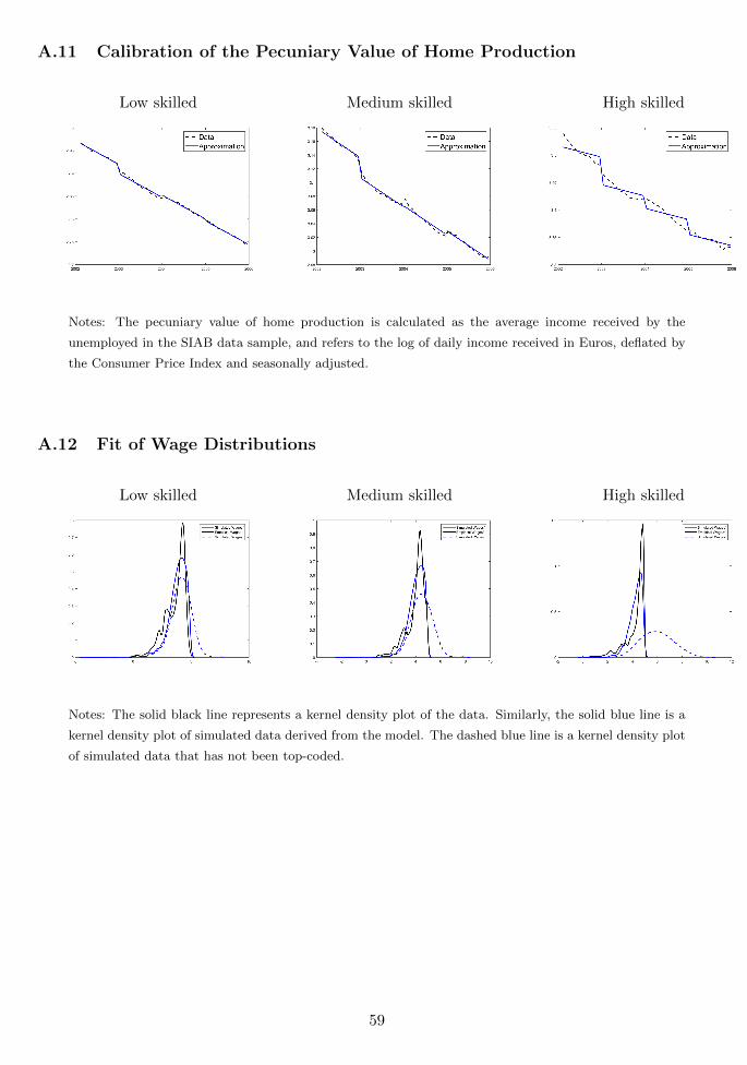
A.11 Calibration of the Pecuniary Value of Home Production

Low skilled Medium skilled High skilled

Notes: The pecuniary value of home production is calculated as the average income received by the

unemployed in the SIAB data sample, and refers to the log of daily income received in Euros, deflated by

the Consumer Price Index and seasonally adjusted.

A.12 Fit of Wage Distributions

Low skilled Medium skilled High skilled

Notes: The solid black line represents a kernel density plot of the data. Similarly, the solid blue line is a

kernel density plot of simulated data derived from the model. The dashed blue line is a kernel density plot

of simulated data that has not been top-coded.

59

labor market reforms: an evaluation of the hartz …sarkoups.free.fr/bradleykugler19.pdfmarket e...

Documents