the financial feasibility analysis of municipal solid...
TRANSCRIPT

THE FINANCIAL FEASIBILITY ANALYSIS OF MUNICIPAL SOLID WASTE TO ETHANOL
CONVERSION
By
Osamu Sakamoto
PLAN B MASTER RESEARCH PAPER
Submitted to Michigan State University
in partial fulfillment of the requirement for the degree of
MASTER OF SCIENCE
Department of Agricultural Economics
2004

ABSTRACT
THE FINANCIAL FEASIBILITY OF MUNICIPAL SOLID WASTE TO ETHANOL CONVERSION
By
Osamu Sakamoto
Lignocellulosic portion of municipal solid waste (MSW) is considered a potential
feedstock for fuel ethanol production. I review the trends in MSW generation,
composition and disposal practices, and evaluate the aggregate and regional potential of
MSW as a feedstock. I present an overview of the current technology of MSW to ethanol
conversion. An attractive feature of MSW-ethanol conversion is that the feedstock is
available at a negative cost; i.e. disposal facilities charge tipping fees ranging from $15-
$100/ton to accept MSW. I assess the financial feasibility of a typical MSW-ethanol plant
with a capacity of 500 tons per day under a number of scenarios with respect to tipping
fees, ethanol prices, capital costs, byproduct prices and ethanol tax incentives. I find the
profitability to be robust across scenarios. I then discuss technical, economic,
environmental and social barriers that inhibit commercialization.

i
ACKNOWLEDGEMENTS
I would like to extend my appreciation to Dr. Satish Joshi, my major professor,
with all respect for his making this research available to me, for his quick feedback for
my analysis and revising all of my drafts, and for his enormous supervision. I express
thanks to Dr. Sandra Batie and Dr. Patricia Norris from the Department of Community,
Agriculture, Recreation and Resource Studies for the support as my committee members.
I am grateful to the General Motors and Engineering Research Council, Canada,
for providing funding for this research through a grant to Dr. Joshi. I have learnt a great
deal from the research fellows from the University of Toronto and Carnegie Mellon
University, who worked with me and gratefully acknowledge my debt to them. Also, I
thank to Xueyan Wang, a research fellow from Michigan State University, who takes
time for me to exchange ideas to develop research methods with long standing friendship.
I must acknowledge James Titmas, the Chief Executive Officer of GeneSyst
International, Inc., who is generous in providing me massive amounts of economic data
of a municipal solid waste (MSW) into ethanol plant. I am grateful to his patience for my
iterative questions with regard to waste to ethanol industry. I also extend appreciation to
Jacqueline Broder from the Tennessee Valley Authority, who provided many reports of
laboratory scale and pilot plant scale economic feasibility analysis of MSW-ethanol
production.
I also would like to thank a number of friends in Michigan State University,
including graduate students of the Department of Agricultural Economics, who have
encouraged me to write thesis. I am particularly grateful to Masanori Fujimoto and Naoki
Okumura who have assisted me in challenging me with alternative view. I also thank

ii
Paul Babladelis and Perry Campbell who reviewed my thesis and corrected English with
thoughtful comments.
I express thanks to my host family: Capes in Columbus Ohio and Halls in
Cleveland Ohio for their spiritual support at opportune times. I must thank my girlfriend,
Naoko in Japan, for her patience and forbearance while I have spent hundreds of hours
working on this research in the United States. Last, I extend sincere appreciation to my
parents, sisters, and all of my family for their understanding and for making it possible
for me to study at Michigan State University.
iii
TABLE OF CONTENTS
LIST OF TABLES......................................................................................... vi LIST OF FIGURES ..................................................................................... viii ABBRIVIATION............................................................................................ x CHAPTER I INTRODUCTION .......................................................................................... 1
1.1 Problem Statement .................................................................................................... 1 1.2 Research Objective ................................................................................................... 4 1.3 Thesis Outline ........................................................................................................... 5
CHAPTER II THE OVERVIEW OF ETHANOL MARKET .............................................. 6
2.1 Data ........................................................................................................................... 6 2.2 U.S. Ethanol Supply.................................................................................................. 6 2.3 MTBE Ban................................................................................................................ 9
2.3.1 History of Ethanol and MTBE ........................................................................... 9 2.3.2 Economic Advantage and Disadvantage of Ethanol over MTBE .................... 13
2.4 U.S. Ethanol Consumption ..................................................................................... 15 2.4.1 Historical Ethanol Oxygenate Consumption ................................................... 15 2.4.2 Historical Ethanol Consumption as Alternative Fuel...................................... 16
2.5 Regional Ethanol Production and Consumption..................................................... 19 2.6 Transportation Problem .......................................................................................... 23 2.7 Ethanol Market Structure........................................................................................ 26 2.8 Concluding Remarks............................................................................................... 28
CHAPTER III MSW BIOMASS FEEDSTOCK AVAILABILITY .................................... 31
3.1 Data ......................................................................................................................... 32 3.2 Trends in National MSW........................................................................................ 33
3.2.1 Trend of MSW Generated, Landfilled, Incinerated, and Recycled .................. 33 3.2.2 Trend in Landfills............................................................................................. 35 3.2.3 Trend of Tipping Fee ....................................................................................... 38
3.3 MSW Components Convertible to Ethanol ............................................................ 40 3.3.1 Total Lignocellulosic Composition in MSW .................................................... 40 3.3.2 Paper and Paperboard .................................................................................... 44 3.3.3 Wood, Yard Trimmings, and Food Scraps....................................................... 46
3.4 Comparison of Previous MSW Composition Surveys............................................ 48 3.5 Regional MSW Biomass Availability..................................................................... 50

iv
3.6 Concluding Remarks............................................................................................... 54 CHAPTER IV TECHNOLOGY AND POTENTIAL PRODUCTS YIELD ....................... 57
4.1 Molecular Mechanism of Biomass-Ethanol Conversion Process........................... 58 4.2 Processing Steps...................................................................................................... 60
4.2.1 MSW Classification.......................................................................................... 62 4.2.2 Hydrolysis ........................................................................................................ 62 4.2.3 Fermentation.................................................................................................... 65 4.2.4 Distillation ....................................................................................................... 65 4.2.5 Processing Steps by GeneSyst.......................................................................... 66
4.3 Technological Description of GPV......................................................................... 67 4.4 Potential Ethanol Yield ........................................................................................... 69
4.4.1 Theoretical Assumption ................................................................................... 69 4.4.2 Assumptions in the Field .................................................................................. 73
4.5 Potential By-Product Yield ..................................................................................... 75 4.5.1 Assumption in the Field ................................................................................... 75 4.5.2 Description of By-Products.............................................................................. 76
4.6 Concluding Remarks............................................................................................... 79 CHAPTER V ECONOMICS OF MSW-ETHANOL PRODUCTION............................... 80
5.1 Data ......................................................................................................................... 80 5.2 Estimate of MSW-Ethanol Plant Economics.......................................................... 81
5.2.1 Net Profit Function Model ............................................................................... 81 5.2.2 Ethanol Sales ................................................................................................... 82 5.2.3 Sales of Recovered Material ............................................................................ 83 5.2.4 Chemical By-Product Revenue ........................................................................ 84 5.2.5 Feedstock Cost ................................................................................................. 85 5.2.6 Direct Cost ....................................................................................................... 86 5.2.7 Indirect Cost..................................................................................................... 87 5.2.8 Annual Net Profit ............................................................................................. 87
5.3 Cash Flow Analysis ................................................................................................ 88 5.3.1 Methodology .................................................................................................... 88 5.3.2 Capital Cost ..................................................................................................... 90 5.3.3 Capital Charges ............................................................................................... 92 5.3.4 Government Incentive ...................................................................................... 93 5.3.5 Economic Premises .......................................................................................... 95 5.3.6 Base Case Economic Evaluation ..................................................................... 97
5.4 Partial Sensitivity Analysis ..................................................................................... 98 5.4.1 Methodology .................................................................................................... 98 5.4.2 Change in Ethanol Price and Tipping Fee ...................................................... 99 5.4.3 Change in Capital Cost.................................................................................. 101 5.4.4 Change in Technological Efficiency .............................................................. 104 5.4.5 Effect of Collocation ...................................................................................... 106 5.4.6 Changing Price of By-Product....................................................................... 108

v
5.5 Economic and Political Obstacles......................................................................... 108 5.5.1 Competition.................................................................................................... 109 5.5.2 Public Acceptance.......................................................................................... 111
5.6 Concluding Remarks............................................................................................. 113 CHAPTER VI CONCLUSION AND RESEARCH RECOMMENDATION ................... 115 APPENDICES ............................................................................................ 120 BIBLIOGRAPHY....................................................................................... 143

vi
LIST OF TABLES
Table 2.1 The MTBE Ban Schedule ................................................................................. 12 Table 2.2 Historical MTBE consumption in the U.S. (million gallons) ........................... 23 Table 2.3 Total Freight Costs for Ethanol Transportation for 5 BGY by 2012 Scenario
(million 2000 dollars) ............................................................................................... 26 Table 2.4 Total Estimated Capital Investment for Terminal Improvements and Retail
Conversion for E10/E5.7 for 5 BGY by 2012 Scenario (million 2000 dollars) ....... 26 Table 3.1 Trend of MSW Generation, Recycling, and Landfilling in 1960-2000............ 34 Table 3.3 Summary of Total Landfilled MSW Component in the US in 2000. ............... 43 Table 3.4 Paper and Paperboard Generation in MSW, 2000............................................ 45 Table 3.5 Comparison of MSW Composition Survey ...................................................... 50 Table 4.1 Technological Efficiency of Biomass to Ethanol Conversion.......................... 60 Table 4.2 Estimated Feedstock Requirements for Various-Sized Biomass-Ethanol Plant72 Table 4.3 Estimated Ethanol Yield per Ton of MSW....................................................... 73 Table 4.4 Yield of Marketable Chemical Product per ton of MSW by Material Balance
Survey by GeneSyst.................................................................................................. 76 Table 5.1 Summary of Market and Salvage Value of Products........................................ 84 Table 5.2 EBITDA of MSW-Ethanol Production in 500 TPD Case ................................ 88 Table 5.3 Estimate of Facility Construction Cost............................................................. 91 Table 5.4 Annual Depreciation of Capital ........................................................................ 92 Table 5.5 Ethanol Incentives by State............................................................................... 95 Table 5.6 Comparison of Capital Cost Estimate............................................................. 104 Table A.1 Summary of Tipping Fee and Waste Volume by Region and Facility Type. 121 Table A.2: Summary of 745 Landfill Data ..................................................................... 122 Table A.3 OLS Regression Results ................................................................................ 125 Table B.1 MSW Generation, Recycling, Landfilled by State in the U.S. in 2003 ......... 126 Table B.2 MSW Density of Top 20 U.S. Populated Metropolitan Area ........................ 130 Table D.1 Revenue Schedule of a 500 TPD MSW-Ethanol Plant at the Base Case (U.S.
Thousands Dollar)................................................................................................... 132 Table D.2 Cost Schedule of a 500 TPD MSW-Ethanol Plant at the Base Case (U.S.
Thousands Dollar)................................................................................................... 133 Table D.3 Cash Flow of a 500 TPD MSW-Ethanol Plant under Different Tax Program
Scenario (U.S. Thousands Dollar) .......................................................................... 134 Table D.4 IRR Sensitivity with Changing Ethanol Price and Tipping Fee (EBITDA).. 135 Table D.5 IRR Sensitivity with Changing Ethanol Price and Tipping Fee (After Tax; No
Tax Incentive case) ................................................................................................. 136 Table D.6 IRR Sensitivity with Changing Ethanol Price and Tipping Fee (After Tax; Tax
Incentives Ends in Year 15).................................................................................... 137 Table D.7 NPV Sensitivity with Changing Ethanol Price and Tipping Fee (EBITDA; U.S.
Million Dollar) ........................................................................................................ 138

vii
Table D.8 NPV Sensitivity with Changing Ethanol Price and Tipping Fee (Scenario 1; U.S. Million Dollar)................................................................................................ 139
Table E.1 Time Line of MSW-Ethanol Project of PMO in the City of Middletown, NY................................................................................................................................. 142

viii
LIST OF FIGURES
Figure 2.1 Trends of Domestic Ethanol Productions in the US.......................................... 8 Figure 2.2 RFG Program Areas .......................................................................................... 9 Figure 2.3 Monthly Ethanol and MTBE Production in 1997-2003 in the U.S................. 12 Figure 2.4 Monthly Average Corn Farm Price Received in Illinois................................. 14 Figure 2.5 Trends of Gasoline Price and Retail Ethanol Price ......................................... 14 Figure 2.6 Trend of Ratio of Unleaded Fuel Price to Corn Price ..................................... 15 Figure 2.7 Historical Ethanol and MTBE consumption as an Oxygenates ...................... 16 Figure 2.8 California Ethanol Consumption in 2000 and Projected Consumption in 2003-
2005........................................................................................................................... 16 Figure 2.9 Trends of Alternative Fuel Consumption in the U.S. ...................................... 18 Figure 2.10 Trends of Number of Vehicle using Alternative Fuel in the U.S. ................. 19 Figure 2.11 Map of Ethanol Plants in the U.S. ................................................................. 21 Figure 2.12 Ethanol Consumption by Region in 2000 in the U.S. ................................... 21 Figure 2.13 MTBE Consumption by Region in 2000 in the U.S...................................... 22 Figure 2.14 Top Eight U.S. Ethanol Producers by Production Capacity (2002) .............. 28 Figure 3.1 Trend of MSW Generation per Capita and SWM in the U.S.......................... 35 Figure 3.2 Percentage of SWM in 2000............................................................................ 35 Figure 3.3 Trend of Number of Landfills in the U.S. ....................................................... 37 Figure 3.4 Trend of Landfill Ownership........................................................................... 38 Figure 3.5 Trend of MSW Volume Managed by Ownership ........................................... 38 Figure 3.6 Trend of Tipping Fee in the U.S. (Dollar per ton)........................................... 40 Figure 3.7 Lignocellulosic Compositions in MSW in the U.S. in 2000 ........................... 42 Figure 3.8 Lignocellulosic Compositions in Landfilled MSW in the U.S. in 2000 ......... 43 Figure 3.9 Trends of Paper & Paperboard Generation, Recycling, and Landfilling ........ 45 Figure 3.10 Trends of Wood Generation, Recycling, and Landfilling ............................. 47 Figure 3.11 Trends of Food Scraps Generation, Recycling, and Landfilling ................... 48 Figure 3.12 Trends of Yard Trimming Generation, Recycling and Landfilling............... 48 Figure 4.1 Conversion Process from Cellulose to Ethanol ............................................... 58 Figure 4.2 Glucose Fermentation...................................................................................... 59 Figure 4.3 Xylose Fermentation ....................................................................................... 60 Figure 4.4 Processing Steps of MSW-Ethanol Plant ........................................................ 61 Figure 4.5 Sugar compositions of Poplar Sawdust, Corn Stover, and Bagasse................ 70 Figure 5.1 Pie Chart of Revenue Source of MSW-Ethanol Production in 500 TPD Case88 Figure 5.2 Effect of Ethanol Price on IRR...................................................................... 101 Figure 5.3 Effect of Tipping Fee on IRR........................................................................ 101 Figure 5.4 Effect of Capital Cost on IRR ....................................................................... 102 Figure 5.5 Effect of Ethanol Yield on IRR..................................................................... 105 Figure 5.6 Effect of Efficiency Factor on IRR ............................................................... 106 Figure 5.7 Effect of Waste Transportation Cost on IRR ................................................ 108 Figure A.1 Distribution of Tipping Fee Charged by MSW Disposing Facility ............. 123 Figure B.1 Distribution of the U.S. Population in 2000 ................................................. 128

ix
Figure B.2 Distribution of MSW in the U.S. in 2000..................................................... 129 Figure C.1 Cellulose Conversion by GPV...................................................................... 131 Figure D.1 Effect of Furfural Price on IRR .................................................................... 141 Figure D.2 Effect of Aluminum Price on IRR................................................................ 141

x
ABBRIVIATION
ADM (Archer Daniels Midland) AEO2000 (Annual Energy Outlook 2000) ARI (Alternative Resource, Inc.) BDT (Bone-dry ton) BGY (Billion gallons per year) CAAA90 (The Clean Air Act Amendments of 1990) CFDC (Clean Fuel Development Coalition) CG (Conventional gasoline) CNG (Compressed natural gas) CO (Carbon monoxide) CO2 (Carbon dioxide) Cu.Yd. (Cubic yard) C/D (Construction and Demolition) DAI (Downstream Alternative, Inc.) DOE (Department of Energy) EBITDA (earning before interest, tax, depreciation and amortization) EIA (Energy Information Administration) EPA (Environmental Protection Agency) GAO (General Accounting Office) GPV (Gravity Pressure Vessel) GSA (General Service Administration) IRR (Internal rate of return) LNG (Liquefied natural gas) LPG (Liquefied petroleum Gases) MGY (Million gallons per year) MRF (Material recovery facility) MSW (Municipal solid Waste) MT (Metric ton) MTBE (Methyl tertiary butyl ether) NAAQS (the National Ambient Air Quality Standard) NESCAUM (Northeastern States for Coordinated Air Use Management) NOx (Nitrogen oxide) NPV (Net present value) NREL (National Renewable Energy Laboratory) N/A (No data is available) OLS (Ordinary least square) PADD (Petroleum Administration of Defense District) PMO (Pencor-Masada OxyNol) PPI (Producer Price Index) RCRA (Resource Recovery Act)

xi
RFA (Renewable Fuel Association) RFG (Reformulated gasoline) SSCF (Simultaneous saccharification and co-fermentation) SWM (Solid waste management) TS (Transfer station) TPD (Tons per day) TVA (Tennessee Valley Authority) USDA (U.S. Department of Agriculture) WRBEP (Western Regional Biomass Energy Program) WTE (Waste-to-energy facility)

1
CHAPTER I
INTRODUCTION
1.1 Problem Statement
Ethanol blended gasoline is currently used as a cleaner burning automobile fuel in
the United States. The Clean Air Act Amendments of 1990 (CAA90) mandated the use
of reformulated or oxygenated gasoline in many urban areas in the United States. While
ethanol and methyl tertiary butyl ether (MTBE) have been the two most common
oxygenates, MTBE is more widely used due to relatively lower production cost.
Moreover, ethanol is mostly produced in the Corn Belt Area of the Midwest, far from the
major gasoline consumption urban centers. The critical shortcoming of ethanol is that it
cannot be transported through pipelines. Hence, high transportation costs prevent
increasing consumption of ethanol on the East and West coasts.
In a recent turn, however, MTBE is now seen as a suspected carcinogen that
moves quickly through bedrock into underground water supply, giving it taints the water
and has a distinct odor (Broder et al. 2001; U.S. EPA 2004a). For this reason, 14 States
have banned the use of MTBE in transportation fuels. MTBE was to be phased out in
California beginning in 2003 (Dipardo 2002; RFA 2001a; GAO 2002). However, the
state government announced the decision to delay the ban until 2004, in part to keep
California's consumer gasoline prices from skyrocketing, and also to protect the state
from facing another energy crisis. This phase out leaves ethanol as the leading candidate
to replace MTBE. Taking the issues associated with national security and the balance of
trade deficit of oil from the Middle East into consideration, demand is projected to

2
increase steadily over the next two decades (EIA 2004a; California Energy Commission
2001a; Hutzler 2003).
Most of the projected increase in ethanol demand in the short run is likely to be
met by corn-based ethanol, produced in the Midwest. However, current technology
allows cellulose contained in various kinds of biomass to be converted to ethanol.
Significant amounts of cellulosic biomass, in the form of paper and paper products, is
currently disposed in landfills or burned. Given this, in order to meet projected increase
in ethanol demand, a good deal of attention is now being paid to biomass to support the
corn-based ethanol. In other words, we can make use of this cheap abundant waste as an
input for ethanol production.
Biomass wastes that can be converted to ethanol include agricultural residues
(e.g., rice straw or sugar cane bagasse), forestry residues, and biomass components in
municipal solid waste (MSW). The benefit gained by ethanol is not limited to an increase
in ethanol production. MSW-ethanol conversion can be an alternative waste disposal
process. In both industrialized and developing countries, MSW has been buried on land,
or burned, as the final disposal process. Both methods have significant environmental
impacts through air, water, and ground pollution. Although the U.S. has much more
abundant landfill space, land scarcity is observed in populated urban areas. Because
approximately 90% of MSW could be reused by available technology (GeneSyst 2004;
Masada 2004), MSW-to-ethanol conversion would be a promising approach to reducing
the material in landfills and to extend landfill life.
A few previous studies have analyzed the costs and benefits of biomass-to-ethanol
conversion. Several private and public organizations have surveyed regional biomass

3
availability and feasibility of ethanol production. For example, the California Energy
Commission estimates the potential statewide ethanol production from available biomass,
including MSW, in California (2001b). Motivation of the study is largely a result of the
impending ban of MTBE. The state of Hawaii (1994) began researching biomass
availability and the technological feasibility of biomass-ethanol conversion at an early
date in an effort to reduce heavy dependence on oil imports. BBI International (2003)
estimated the potential economic impact of biomass-ethanol production, such as
employment impact in Hawaii. Mann and Bryan (2001) also addressed the feasibility of
producing ethanol from various kinds of biomass available in northeastern North Dakota
and northwestern Minnesota as a part of the Western Regional Biomass Energy Program
(WRBEP).
However, the vast majority of these previous studies focused on agricultural
residues or dedicated energy crops expressly produced as an input for ethanol production.
And only a few have analyzed MSW to ethanol conversion. This is largely because of the
technological uncertainties and the limited data sources about the recycling market,
conversion process, and possible benefit and costs related to this infant industry.
The Tennessee Valley Authority (TVA) initially conducted an economic analysis
of a proposed MSW-ethanol plant in Muscle Shoals in Alabama between 1990 and 1992,
and found that the profitability was not positively robust, but was economically feasible
(Broder et al. 1993). However, since the time of TVA’s analysis, technological efficiency
of cellulose-ethanol conversion has dramatically improved. Fox et al. (1999) analyzed the
feasibility of regional MSW based ethanol production in the city of Phoenix, in Maricopa
County, Arizona, in the part of WRBEP with state-of-art technology using a gravity

4
pressure vessel (GPV). However, estimates of plant economics were site-specific and
they did not assess nation-wide potential for MSW-ethanol conversion.
Now the technology is ripe. In fact, three private firms, Pencor-Masada OxyNol
(PMO) in the city of Middletown in Orange County, New York, GeneSyst International
Inc. in the city of Canton in Stark County, Ohio, and Genahol-Arizona Inc. in the city of
Phoenix in Maricopa County, Arizona, are planning to begin operation on a commercial
scale in near future. Thus, this research, assessing financial feasibility of this infant
industry, is timely.
1.2 Research Objective
The key to succeed in MSW-ethanol industry is “profitability.” This research is
aimed to provide a comprehensive analysis of financial feasibility of MSW-ethanol
production at a national scale with the current best available technology.
To begin with, sustainable input flow should be guaranteed to maintain business.
To attack this question, the paper initially studies the trend of MSW generation,
recycling, and landfilling in the U.S. Then, the paper determines not only aggregate
MSW availability, but also the lignocellulosic composition in MSW that is convertible to
ethanol. Equally important, regional MSW availability will be addressed. The paper
identifies regions that can supply enough MSW for an ethanol plant to maintain business.
Second, the paper analyzes the financial feasibility of MSW-ethanol production.
To carry out this analysis the potential yield of ethanol and a set of by-products per ton of
MSW should be known. The next step is modeling a firm’s profit function by taking
potential revenue sources and costs, related to production, into account. Timing of cash

5
outflows and inflows is also important for a firm’s investment decision. Cash flow is
estimated over the entire economic life of the plant. Next, the key economic parameters,
which are significant in determining plant economics, are identified and the robustness of
profitability is analyzed with respect to variations in these parameters. Last, technical,
economic, political barriers that inhibit commercialization are discussed.
1.3 Thesis Outline
This thesis consists of five parts. Chapter II provides the overview of the current
ethanol market. In the last section of Chapter II, the advantage of MSW-ethanol
production over traditional corn-starch based production is summarized. Further
discussion about how it can contribute to currently rapidly growing demand for ethanol is
also included. Chapter III examines MSW biomass availability. Although there are
substantial differences in terms of MSW composition by region and season, it provides an
approximate range of MSW lignocellulosic compositions. Also, the distribution of MSW
across the U.S. is presented. Chapter IV describes state-of-art technology and the
operational steps of MSW-ethanol production. Moreover, it discusses the potential yield
of ethanol and by-products based on the theory, laboratory-based and assumptions by the
plants in the field. Chapter V, the core chapter of this thesis, analyzes profitability of
ethanol conversion. Plant economics, the base case, are estimated based on the data by
Titmas (2004), and sensitivity analysis is performed. Chapter VI is the concluding
chapter that presents a summary of all research and suggests further research
recommendations.

6
CHAPTER II
THE OVERVIEW OF ETHANOL MARKET
The purpose of this chapter is to provide an overview of the ethanol market. It is
important to identify how MSW-ethanol producers can play as niche players in the clean
fuel energy industry. The key issues to address this question are (1) the trend of national
ethanol supply and demand, (2) the potential effect of a coming MTBE ban, (3) ethanol
supply and demand across the U.S. region by region, (4) ethanol transportation problems,
and (5) current ethanol market structure. The research results are presented in the above
order. Finally, I provide a summary on how MSW based ethanol producers can contribute
to the ethanol market.
2.1 Data
The main source for secondary data is from the Energy Information
Administration (EIA) in the U.S. Department of Energy (DOE) and Renewable Fuel
Association (RFA). These organizations estimate and report data on the United States’
ethanol and MTBE production on a monthly and yearly basis. Furthermore, EIA provides
data on national and regional ethanol consumption as oxygenate, and as an alternative
fuel to conventional gasoline (CG).
2.2 U.S. Ethanol Supply
Ethanol use began to boom in the early 1970s, when oil supply disruptions in the
Middle East affected U.S. national security. In addition, our growing concern for a clean

7
environment became a driving force to eliminate lead (an octane booster) from gasoline.
Lead is a cumulative toxin that builds up in soft tissue, such as kidneys, bone marrow,
liver, brain bones, and teeth. Lead can be extremely damaging, especially for children,
because it inhibits the body's oxygen and calcium transport and alters nerve transmission
in the brain. Lead poisoning can cause mental retardation, impaired growth, and, at high
doses, even death. The advent of the environmental movement in the 1970s hit the
gasoline market when the U.S. Environmental Protection Agency (U.S. EPA) issued
restrictions on the use of lead in fuel in 1978. Over the next ten years various levels of
regulation resulted in a phase down of lead levels in gasoline. Ethanol and MTBE are the
two common chemicals used to enhance gasoline's oxygen and octane content. Ethanol
has been commonly used by blending it directly into gasoline in a mix of 10% ethanol
and 90% gasoline, called “gasohol” or “E10” (DOE 2003).
Ethanol production in the U.S. increased considerably in two decades. While only
175 million gallons were produced in 1980, the ethanol supply has skyrocketed to
approximately 2.6 billion gallons by 2003 (Figure 2.1). This success in the ethanol
industry is attributed to CAA90, which mandating the use of oxygenated gasoline in
certain geographical areas not meeting the National Ambient Air Quality Standard
(NAAQS) for carbon monoxide (CO). The main source of CO emissions is the
combustion engine. While many types of these engines are used in products such as
lawnmowers, chain-saws, and other gasoline powered equipment, the primary source of
ambient CO in most areas is motor vehicles.
Designed to increase combustion efficiency, oxygenated gasoline was viewed by
the government as a practical way to help reduce CO emissions. Two programs have

8
been implemented to achieve the goals under CAA90. The Oxygenated Fuel Program
(Oxyfuel Program) is in effect only during fall and winter months in certain urban areas
to reduce CO emissions. It has been a tremendous success, with the number of non-
attainment areas decreasing by two-thirds since 1990, and areas continue to demonstrate
attainment each year. The Reformulated Gasoline Program (RFG Program) requires the
use of oxygenated fuel on a year-round basis in metropolitan areas with high levels of CO
and ground-level ozone.
Ethanol is already used in Federal RFG in populated metropolitan areas such as
Chicago and Milwaukee (Figure 2.2). The Oxyfuel Program requires a minimum oxygen
content of 2.7% in non-attainment areas, and the RFG Program requires 2% oxygen
content. The two most common ways of boosting oxygen levels to the required Oxyfuel
levels are to add either 15% MTBE or 7.5% ethanol to gasoline (ethanol required to be
blended into gasoline is as half of MTBE because ethanol has higher oxygen content than
MTBE).
Figure 2.1 Trends of Domestic Ethanol Productions in the US Source: 1980-2000 by RFA (2001a) and 2001-2003 by EIA (2004b)
0.0
0.5
1.0
1.5
2.0
2.5
3.0
1980 1982 1984 1986 1988 1990 1992 1994 1996 1998 2000 2002Year
billi
on g
allo
s per
yea
r

9
Figure 2.2 RFG Program Areas Source: U.S. EPA, 2004b
2.3 MTBE Ban
2.3.1 History of Ethanol and MTBE
Recently, MTBE has become quite controversial. Claims have been made that
MTBE has caused widespread contamination of drinking water wells, which can result in
adverse health effects, including cancer, to consumers of MTBE contaminated water.
Concern over the use of MTBE in gasoline began to grow with the detection of the
chemical at low levels in groundwater nationwide; especially when it was found in
relatively high levels in some municipal water supply wells (U.S. EPA 2004a). High
profile cases, such as the closure of the Santa Monica, California well field and

10
contamination of the public wells in South Tahoe, California. brought national attention
to this issue.
MTBE is more soluble in water than any other gasoline component. It is 30 times
more soluble than benzene. When MTBE is released into the soil as a result of a spill or
leak it may separate from the rest of the gasoline, lead the plume to the groundwater, and
dissolve rapidly once there. MTBE travels at the same rate as groundwater and is
therefore often the leading edge of any petroleum plume. This puts receptors at a greater
risk of MTBE contamination when gasoline leaks occur. On the other hand, ethanol has
high solubility but is biodegradable. Thus, it degrades into harmless byproducts before it
reaches any potential receptor.
On March 25, 1999, Governor Gray Davis released Executive Order D-5-99,
which ordered the removal of the additive MTBE from California gasoline at the earliest
possible date, but no later than December 31, 2002. In addition to the State of California,
sixteen other states also plan to phase out MTBE use at a state level (Table 2.1). On
December 13, 1999, Chicago became the first city to ban MTBE when city council
unanimously voted to ban the petroleum-based oxygenate (Ames 2001). As long as the
Federal requirement for 2% oxygen in RFG continues in all states, ethanol (as a substitute
good for MTBE) will replace MTBE. At the same time, these regulations initiated by
those states created incentives to the ethanol industry to expand production in order to
prepare for growing demand after the law is enacted. Figure 2.3 shows monthly ethanol
and MTBE domestic production during 1997-2003. Obviously, ethanol production
capacity rapidly grew while MTBE production diminished. Growth in 2002 was
particularly remarkable in that ethanol production eventually exceeded MTBE production

11
by 2003. The growth of ethanol is expected to increase steadily for at least another couple
of decades (EIA 2004a; Hutzler 2003; DiPardo 2002; RFA 2001a; California Energy
Commission 2001b).
While ethanol will take the place of MTBE, it has not yet been competitive with
fossil fuel. Current ethanol producers are largely supported by government subsidies. The
U.S. Congress passed the National Energy Act of 1978, which gave a Federal tax
exemption for gasoline containing 10% ethanol. The Federal subsidy, now at $0.52 per
gallon, allows the price of ethanol to remain close to the price of CG. However, if another
alternative fuel is found to be more economically and environmentally efficient by
technological development in future, the tax incentive programs above could expire.
Congress is now debating an amendment to the Energy Bill in which MTBE will be
completely eliminated from all gasoline in the United States. The amendment, which still
must be part of the final Senate Energy Bill passed and signed by President Bush, would
boost the use of renewable energy fuel including ethanol to five billion gallons by 2012
(Abbott 2003). Thus, the long-term ethanol production growth in the near future heavily
depends on government policy.

12
Table 2.1 The MTBE Ban Schedule
State MTBE Ban Schedule MTBE
Consumption (% of U.S. total)
California MTBE started January 1, 2004 (Firstly announced to ban in December 31, 2002, but postponed)
31.7
Colorado MTBE ban started April 30, 2002 0 Connecticut MTBE ban started October 1, 2003 3.1 Illinois MTBE prohibited by July 2004 0 Indiana MTBE limited to 0.5% by volume, starting July 23, 2004 0 Iowa 0.5% MTBE by volume cap, already in effect 0 Kansas MTBE limited to 0.5% by volume, starting July 1, 2004 0 Kentucky MTBE ban starting January 1, 2006; beginning in January 1, 2004,
ethanol encouraged to be used in place of MTBE 0.8
Maine Law merely expresses state’s “goal” to ban MTBE; it is not an actual ban. The “goal” is to phase out gasoline or fuel products treated with MTBE by January 1, 2003
0
Michigan MTBE prohibited by June 1, 2003 0 Minnesota All ethers (MTBE, ETBE, TAME) limited to 1/3 of 1.0% by weight after
July 1, 2000; after July 1, 2005, total ether ban 0
Missouri MTBE limited to 0.5% by volume, starting July 1, 2005 1.1 Nebraska MTBE limited to 1.0% by volume, starting July 13, 2000 0 New York MTBE ban started January 1, 2004 7.5 Ohio MTBE ban starting July 1, 2005 0 South Dakota 0.5% MTBE by volume cap, already in effect 0 Washington MTBE ban started December 31, 2003 0 Source: EIA, 2002a
Figure 2.3 Monthly Ethanol and MTBE Production in 1997-2003 in the U.S. Source: EIA, 2004b
0
50
100
150
200
250
300
Jan-
97
Jul-9
7
Jan-
98
Jul-9
8
Jan-
99
Jul-9
9
Jan-
00
Jul-0
0
Jan-
01
Jul-0
1
Jan-
02
Jul-0
2
Jan-
03
Jul-0
3
Thou
sand
s Bar
rels
per
day
Ethanol Production MTBE Production

13
2.3.2 Economic Advantage and Disadvantage of Ethanol over MTBE
One of the major disadvantages of ethanol over MTBE is that its production is
sensitive to change in corn prices. In Figure 2.1, ethanol production substantially dropped
in mid-1996. Figure 2.4 points out high corn prices in mid-1996. This was due to wet
conditions resulting in small corn supply and higher corn prices. Unlike MTBE, which
can be produced from a chemical reaction of methanol (derivative of natural gas) and
isobutylene (an oil refinery product), corn based ethanol production is affected by
weather conditions. Note that this is not the case with MSW biomass based ethanol
production. Daily MSW biomass supply is not as sensitive to weather conditions as are
agricultural products.
Although ethanol production is influenced by corn prices, the empirical analysis
states the price of corn has very little to do with the price of ethanol (CFDC 2004).
Ethanol prices are more highly correlated with the price of gasoline and gasoline
blending components (Figure 2.5). Thus, low corn prices do not always indicate low
ethanol prices, and high corn prices do not always indicate high ethanol prices. Holding
the ethanol price constant, a low biomass price enhances the profitability of ethanol
production. To put it another way, as the biomass price increases, profits by ethanol
production diminish.
Figure 2.6 is the historical ratio of unleaded gasoline (proxy for the ethanol price)
to corn price available. The horizontal straight line indicates the historical average price
ratio. The corn based ethanol production is now well above this level. Although it is still
uncertain that price of ethanol will be unchanged in the future because the price is
maintained at a certain level by the Federal and State tax exemption program, the cost

14
reduction by biomass-ethanol production is surely the key factor for the profitability of
the ethanol industry in near term.
Figure 2.4 Monthly Average Corn Farm Price Received in Illinois Source: Farmdoc, 2004
Figure 2.5 Trends of Gasoline Price and Retail Ethanol Price Source: CFDC, 2004
0.0
0.5
1.0
1.5
2.0
2.5
3.0
3.5
4.0
4.5
5.0
Jan-
60
Jan-
63
Jan-
66
Jan-
69
Jan-
72
Jan-
75
Jan-
78
Jan-
81
Jan-
84
Jan-
87
Jan-
90
Jan-
93
Jan-
96
Jan-
99
Jan-
02
Cor
n P
rice
($/B
u)
1.00
1.10
1.20
1.30
1.40
1.50
1.60
1990 1991 1992 1993 1994 1995 1996 1997 1998 1999 2000
Year
$ pe
r ton
Motor Gasoline Price Retail Ethanol Price

15
Figure 2.6 Trend of Ratio of Unleaded Fuel Price to Corn Price Source: Missouri Value Added Development Center, 2001
2.4 U.S. Ethanol Consumption
2.4.1 Historical Ethanol Oxygenate Consumption
Figure 2.7 depicts the historical consumption of both ethanol and MTBE as
oxygenate. Ethanol consumption has not changed much in a decade and was still less
than half of MTBE consumption in 2002. However, after California begins banning all
MTBE use as oxygenate, demand for two oxygenate fuels is expected to be changed, or
will potentially even be reversed. According to the estimate of the U.S. General
Accounting Office (GAO) and the U.S. Department of Transportation (Figure 2.8), an
additional eight million gallons of ethanol will be needed to meet ethanol demand in
California after the phase-out of MTBE.

16
Figure 2.7 Historical Ethanol and MTBE consumption as an Oxygenates Source: EIA, 2002b
Figure 2.8 California Ethanol Consumption in 2000 and Projected Consumption in 2003-2005
Source: GAO, 2002
2.4.2 Historical Ethanol Consumption as Alternative Fuel
Ethanol is not only used as an oxygenate fuel, but also used as an alternative fuel.
Oxygenate use of ethanol, such as E10, is a complement to petroleum, but higher blends,
such as E85 (85%ethanol blending with 15% CG), is a substitute for the petroleum.
0.0
0.5
1.0
1.5
2.0
2.5
3.0
3.5
1993 1994 1995 1996 1997 1998 1999 2000 2001 2002
Year
Bill
ion
gallo
ns
MTBE Ethanol in gasohol
60
870 880 890
0
100
200
300
400
500
600
700
800
900
1000
2000 2003 2004 2005Year
Mill
ion
gallo
ns p
er y
ear

17
Currently, 394 million gallons of fuels are consumed as alternative fuels in the
U.S. Fuels made of natural gas, such as liquefied petroleum gases (LPG), compressed
natural gas (CNC) and liquefied natural gas (LNG) account for roughly 96% of total U.S.
alternative fuel consumption. Natural gas is cheaper and more abundant non-renewable
resource than oil. The U.S. natural gas reserves are expected to last at least 80 years. It is
easier to process than oil, can be easily transported, produces less air pollution and burns
hotter than any other fossil fuel.
However, natural gas has some environmental drawbacks. When it is processed it
releases highly toxic hydrogen sulfide into the air and when it is transported, it could
cause huge explosions. Also, the largest component of natural gas methane is more potent
than carbon dioxide as a greenhouse gas. However, because of its abundance it is useful
as a transition from nonrenewable to renewable energy sources.
Renewable alternative fuels include E85, E95 (95% ethanol), M85 (85%
methanol), M100 (100% methanol). Ethanol as alternative fuel use is not as promising as
blending use in the near term for a few reasons. First, most automobile engines do not
allow the use of E85 fuel. Second, gas stations also do not allow the use of E85 fuel, so a
new infrastructure would be needed to popularize it. Studies of the DOE and the General
Service Administration (GSA) have shown that refueling stations need at least 200 steady
customers for any single grade in order to make profitable use of the facilities. Though
large numbers of flexible-fuel vehicles are being sold, they are spread out over the entire
nation, and achieving a "critical mass" of 200 that use a single refueling station is still
difficult to achieve (U.S. Department of Transportation 2002). Finally, a gallon of ethanol
has only two-thirds the energy content of a gallon of gasoline (Hadder 1997). To be

18
competitive with CG, further engine modifications are necessary in order to make up for
low energy content.
Although there are some drawbacks to ethanol use as an alternative fuel, E85 is
gradually gaining popularity. Figure 2.9 shows historical consumption of alternative fuels
and Figure 2.10 indicates the number of vehicles using alternative fuels (renewable fuels
and electricity). Noticeably, E85 is consumed more than methanol or electricity.
Figure 2.9 Trends of Alternative Fuel Consumption in the U.S. Source: EIA, 2002b
0
2
4
6
8
10
12
1993 1994 1995 1996 1997 1998 1999 2000 2001 2002Year
Mill
ion
Gal
lons
E85 (Ethanol 85%) E95 (Ethanol 95%)M85 (Methanol 85%) M100 (Methanol Neat)Electricity

19
Figure 2.10 Trends of Number of Vehicle using Alternative Fuel in the U.S. Source: EIA, 2002b
2.5 Regional Ethanol Production and Consumption
As mentioned earlier in this chapter, ethanol is now dominantly produced in the
Corn Belt of the Midwest region.1 Figure 2.11 plots ethanol plants on a U.S. map. This
excessive concentration of the ethanol industry in one region results in heavy reliance on
MTBE as an oxygenate fuel outside the Midwest area of the U.S. (Figure 2.6 and 2.7).
Remarkably, about 75% of ethanol is solely consumed in Midwest areas, while other
regions only account for 25% of total ethanol consumption. For MTBE consumption,
Midwest consumption remains at the no more than 2%, and almost all is exclusively
outside of the Midwest region. Thus, in reality, ethanol and MTBE are not competitive in
the market, but divvy up the oxygenate fuel market share by region.
1 All States are divided into four regions (i.e., West, South, Midwest, Northeast) corresponding to the Census Region and Division of U.S. Bureau of the Census (2001). West is AK, AZ, CA, CO, HI, ID, MT, NM, NV, OR, WA, WY, South is AL, AR, DC, DE, FL, GA, KY, LA, MD, MS, NC, OK, SC, TN, TX, VA, WV, Midwest is IA, IL, IN, KS, MI, MN, MO, NE, ND, OH, SD, WI, and Northeast is CT, MA, ME, NH, NJ, NY, PA, RI, VT.
0
10,000
20,000
30,000
40,000
50,000
60,000
70,000
80,000
90,000
1993 1994 1995 1996 1997 1998 1999 2000 2001 2002
Year
Num
ber o
f Veh
icle
E85 (Ethanol 85%) E95 (Ethanol 95%)M85 (Methanol 85%) M100 (Methanol Neat)Electricity

20
Table 2.2 summarizes the historical MTBE consumption in 17 states that plan to
phase out their MTBE use as oxygenate fuel. It is apparent that only 5 out of 17 States
will be affected by state regulation (i.e., California, New York, Connecticut, Kentucky,
and Missouri). It is unlikely that other States will be seriously distressed by a MTBE ban
because 9 out of 12 States are located in the Midwest. Nevertheless, the five states noted
above consume 44.2% of total U.S. MTBE consumption. Especially California, the most
automobile dependent state in the nation, which accounts for 32% of total U.S. MTBE
consumption.
It is a conceivable eventuality that the states that have not yet announced a MTBE
ban will shift to ethanol use to accommodate public opinion. If these states, especially
heavily MTBE dependent states such as Texas and New Jersey, begin to phase-out
MTBE use by regulation, the increase of ethanol demand will be further accelerated.
Similar to California, there is a huge potential market for clean fuels in the Northeastern
states (NESCAUM 1999). These states have such a small number of ethanol plants and
would be driven by necessity to import ethanol from the Midwest in the near future to
meet the boost in ethanol demand.

21
Figure 2.11 Map of Ethanol Plants in the U.S. Source: Frazier, Barnes & Associates, LLC., 2004
Figure 2.12 Ethanol Consumption by Region in 2000 in the U.S. Source: EIA, 2003
74.06%
16.24%
0.22%
9.26%
Northeast
Midwest
South
West

22
Figure 2.13 MTBE Consumption by Region in 2000 in the U.S. Source: EIA, 2003
41.11%
33.34%
1.28%
23.89%Midwest
South
West
Northeast

23
Table 2.2 Historical MTBE consumption in the U.S. (million gallons) 1995 1996 1997 1998 1999 2000 2001 States Enacting MTBE Ban California 71.2 78.8 86.5 97.3 103.6 102.4 79.7 Connecticut 10.6 9.4 10.0 10.0 9.0 8.5 9.4 Kentucky 1.8 2.2 2.4 2.1 2.2 2.2 2.2 Missouri 0.0 0.0 0.0 0.0 2.3 3.3 3.2 New York 22.7 22.0 23.7 24.4 21.4 19.7 21.1 Illinois 3.2 1.0 0.9 0.4 0.0 0.0 0.0 Colorado 0.3 0.3 0.3 0.2 0.1 0.0 0.0 Indiana 0.4 0.1 0.1 0.1 0.0 0.0 0.0 Maine 3.7 3.7 3.7 3.7 0.8 0.0 0.0 Iowa 0.0 0.0 0.0 0.0 0.0 0.0 0.0 Kansas 0.0 0.0 0.0 0.0 0.0 0.0 0.0 Michigan 0.0 0.0 0.0 0.0 0.0 0.0 0.0 Minnesota 0.0 0.0 0.0 0.0 0.0 0.0 0.0 Nebraska 0.0 0.0 0.0 0.0 0.0 0.0 0.0 Ohio 0.0 0.0 0.0 0.0 0.0 0.0 0.0 South Dakota 0.0 0.0 0.0 0.0 0.0 0.0 0.0 Washington 0.0 0.0 0.0 0.0 0.0 0.0 0.0 States Consuming MTBE and not Announcing MTBE Ban Arizona 0.3 0.3 1.8 3.7 3.7 3.6 3.6 Delaware 2.6 2.2 2.6 2.8 3.0 3.0 3.0 Dist. Of Columbia 1.1 0.8 0.9 0.8 0.8 0.8 0.7 Maryland 13.4 10.1 11.2 11.1 11.2 11.7 12.6 Massachusetts 16.2 16.0 16.9 16.4 14.8 16.5 16.8 New Hampshire 2.0 2.1 2.3 2.6 2.6 2.9 3.2 New Jersey 30.7 29.0 31.4 32.6 28.1 26.3 27.1 North Carolina 0.4 0.0 0.0 0.0 0.0 0.0 0.0 Pennsylvania 9.3 8.7 9.2 9.4 8.8 9.3 9.7 Rohde Island 3.8 3.5 3.4 3.5 2.9 2.9 2.6 Texas 25.9 23.7 27.0 29.2 31.2 30.3 30.5 Utah 0.0 0.0 0.1 0.1 0.0 0.0 0.0 Virginia 14.0 11.4 12.3 13.1 13.2 13.6 13.6
United States 233.6 225.3 246.7 263.5 259.7 257.0 239.0 Source: EIA, 2003
2.6 Transportation Problem
The major drawback of ethanol is the high transportation cost, because ethanol
cannot be shipped through pipelines. Although Federal and state tax incentives have
made ethanol producers competitive in the market and economically profitable, high
transportation costs prevent other regions from consuming ethanol. MTBE can be piped
to a refinery, then blended with gasoline, and piped to pumping stations throughout the

24
United States. Generally, pipelines are the fastest and most economical method for
transporting liquids.
There are three main reasons why ethanol cannot be moved through pipelines.
First, ethanol absorbs water and impurities that normally reside in fuel pipelines. Water,
typically containing dirty particles such as rust, separates ethanol and gasoline, and these
dirty particles reduce engine performance (Whims 2002). Therefore, ethanol needs to be
carried by other means and must be blended at the terminal instead of the refinery.
Second, the location of a pipeline is problem. Most of the pipelines in the U.S. run
from the Gulf Coast to the East and West Coasts. Thus, corn based ethanol in the
Midwest needs to be transported to the Gulf Coast for piping. Construction of a new
pipeline connecting the Midwest and other regions is not likely in the near future due to
high establishment costs.
The third and final weakness is the logistical limitation of the existing pipelines.
Compared to the volume of liquids normally shipped via pipelines, ethanol has
insufficient volume. This cannot justify the construction of new pipelines.
Therefore, ethanol must be transported by barge, rail, or truck to fuel stations.
Downstream Alternative, Inc. (DAI) has estimated the possible transportation costs and
capital investment costs when the national production of ethanol is less than five billion
gallons per year (BGY) by 2012 scenario (Table 2.3 and 2.4). DAI’s study has estimated
the shipping cost from PADD (Petroleum Administration for Defense District2) II from
2 The United States is divided by the U.S. DOE into five PADD regions for planning purposes. PADD 1 is the East Coast, including CT, DC, DE, FL, GA, MD, ME, MA, NC, NH, NJ, NY, PA, RI, SC, VA, VT, and WV. PADD 2 is the Midwest, including IA, IL, IN, KS, KY, MI, MN, MN, MS, ND, NE, SD, OH, OK, TN, and WI. PADD 3 is the Gulf Coast, including AL, AR, LA, MS, NM, and TX. PADD 4 is the Rocky Mountain area, including CO, ID, MT, UT, and WY. PADD 5 is the West Coast, including AK, AZ, CA, HI, NV, OR, and WA.

25
other regions. PADD II is not expected to import any of its ethanol. In contrast, PADD I
and V will have to incur a burden of high freight cost ($0.11/gal and $0.13/gal,
respectively) to import most of their ethanol from PADD II. In terms of capital
investment cost, DAI study results show an estimated average national cost of about 8
cents per gallon of ethanol to transport it to markets.
The DAI concludes that the transportation industries could increase capacity to
meet increased ethanol transportation demands without serious risk of sustained supply
disruption (EIA 2002c). However, high shipping costs would become a disturbance in
extending the ethanol market.
Again, this is not true for biomass-ethanol production. Biomass is an abundant
and inexpensive regionally-available renewable resource. Furthermore, in the case of
MSW-ethanol, it substantially reduces freight cost when compared to agricultural or
forest residues based ethanol production. MSW availability is positively related to
population; thus, urban areas have more abundant MSW biomass resources than do rural
areas. These are also the places that ethanol is most needed. Consequently, Ethanol
produced from MSW quickly and easily meets the needs of ethanol demand in urban
areas.

26
Table 2.3 Total Freight Costs for Ethanol Transportation for 5 BGY by 2012 Scenario (million 2000 dollars)
Ethanol imports from PADD II Shipments within PADDS Total
PADD Ethanol shipped (BGY) Ship/
Barge Rail Avg.
(cents/gal.)
Truck Rail Barge Avg.
(cents/gal.)
Total Avg.
(cents/gal.)
I. East Coast 1.3 $57.4 $70.0 9.8 $13.1 - $4.0 1.3 $144.5 11.1 II. Midwest 2.2 - - - $77.9 $12.8 $3.2 4.3 $93.9 4.3 III. Gulf Coast 0.7 $2.6 $35.3 5.4 $8.0 - $0.3 1.2 $46.2 6.6 IV. Rocky Mountain 0.1 - $4.5 4.5 $0.2 - - 0.1 $4.7 4.7 V. West Coast 0.8 $51.1 $32.9 10.5 $17.8 - - 2.2 $101.8 12.7 Total 5.1 $111.1 $142.7 30.2 $117.0 $12.8 $7.5 2.7 $391.1 7.7 Source: Technology and Management Services, Inc., 2002. Data taken by DAI, 2002
Table 2.4 Total Estimated Capital Investment for Terminal Improvements and Retail Conversion for E10/E5.7 for 5 BGY by 2012 Scenario (million 2000 dollars)
PADD
New ethanol volume (BGY)
Cost of new tanks
Cost of tank
conversion
Cost of blending systems
Modifying for rail receipt
Contin-gency
Retail conversions Total
Amortized cost
(cents/gal.)
I. East Coast 1.102 $8.89 $0.65 $24.30 $7.10 $1.26 $6.50 $48.66 0.69II. Midwest 1.072 $5.40 $0.31 $33.00 $5.33 $2.02 $7.44 $53.49 0.78III. Gulf Coast 0.626 $5.74 $0.34 $22.20 $3.55 $1.24 $5.28 $38.34 0.96IV. Rocky Mountain 0.042 $0.75 $0.02 $2.40 $1.07 $0.12 $0.31 $4.66 1.73V. West Coast 0.145 $2.33 $0.06 $4.20 $0.36 $0.24 $1.25 $8.42 0.91
Total 2.987 $23.11 $1.38 $86.10 $17.41 $4.88 $20.78 $153.57 0.80
Source: Technology and Management Services, Inc., 2002. Data taken by DAI, 2002
2.7 Ethanol Market Structure
Another problem for the ethanol industry is the fact that ethanol production is a
highly concentrated industry. Illinois based Archer Daniels Midland (ADM), controls
approximately 40% of all ethanol production in the United States. Since ADM is such a
dominant market power, the concern is that only a few ethanol producers will be able to
expand production to meet demand as long as we rely only on corn-produced ethanol.
Many complain that only ADM can benefit from the banning of MTBE (Pace 2003).
Further, large producers have typically partnered with smaller producers or farm coops to

27
market the smaller producer’s supplies of ethanol; thus, the concentration ratio may
underestimate the actual market concentration.
On the other hand, the GAO forecasts that a MTBE ban attracts new small
producers into the market, and the market share of the large producers is projected to
decline (GAO 2002).
There are both advantages and disadvantages of concentrated ethanol market
structure. One advantage is that the industry can take advantage of economies of scale;
industry could lower unit costs to produce a gallon of ethanol. Moreover, pricing
coordination is easier if fewer firms control most of the market shares.
A disadvantage of the current ethanol market structure is that it discourages
competition. New suppliers tend to be left out of the market so that only the preferences
of a few big agribusiness giants are counted.
There are a few reasons why competition is not emerging. First, ethanol is a
homogeneous commodity. Even though it is made from different feedstocks such as corn,
rice straw, or MSW, it seems identical to consumers. Thus, consumers choose products
mainly based on the price. New suppliers cannot appeal to consumers by differentiating
the market. The second reason is a technological barrier. Ethanol conversion needs high
technology and well-trained employees that are not easily available. Third, small
suppliers cannot afford the enormous initial capital investment cost. Fourth, the fuel
distribution network is controlled by the oil industry, whose products compete with
ethanol. Large oil companies prefer to contract with a few large producers instead of a
number of small ethanol producers.

28
Figure 2.14 Top Eight U.S. Ethanol Producers by Production Capacity (2002) Source: GAO, 2002. Data taken by RFA
2.8 Concluding Remarks
In this chapter I looked at the current ethanol market condition. Ethanol demand
in the near future will rise because of the phase-out of MTBE, especially in California.
Now, I summarize how MSW-ethanol production contributes to the future ethanol
market.
First, ethanol demand is projected to increase. States need to guarantee a
sustainable flow of ethanol with the MTBE ban. Biomass-, including MSW, based
ethanol production is increasingly seen as an important and capable approach to meet the
anticipated boost in ethanol needs. For example, New York and northern New Jersey
need about 391 million gallons of ethanol to replace MTBE. According to Masada, less
than half of New York’s MSW would meet this need (Masada 2004).
0%
5%
10%
15%
20%
25%
30%
35%
40%
45%
ArcherDaniels
Midland(ADM)
MinnesotaCorn
Processors
WilliamsBio-Energy
Cargill, Inc High PlainsCorp.
NewEnergyCorp.
MidwestGrain
ChiefEthanol
Perc
ent o
f tot
al c
apac
ity
Capacity of existing plants and those under constructionCapacity of existing plants

29
Second, the U.S. currently depends excessively on imported oil from other
countries. The U.S. presently imports 56% of its petroleum needs and is expected to
reach 60% by 2010 (EIA 2004a). At the beginning of the 1970s OPEC decreased the
output of oil, which resulted in a dramatic increase in oil prices. The world’s interest in
alternative fuels increased significantly. The aim was to become less dependent on oil
and to reduce the cost of expensive oil imports. Ethanol production reduces the U.S. trade
balance by $2 billion annually (EIA 2004a). It is estimated that if existing landfill
inventories and newly generated MSW were converted to ethanol, as much as 25% of oil
and gasoline resources could be saved and used in industry or power generation.
(GeneSyst 2004)
Third, corn-based ethanol production is sensitive to corn prices. Corn-ethanol
plants face ceaseless uncertainty about meteorological factors. Thus, excessive
inclination to corn-based production could result in a shortfall of the ethanol supplies. A
biomass-based ethanol plant, on the other hand, generally deals with more than two
biomass inputs for ethanol production. MSW is a mixture of miscellaneous waste,
including biomass that it is not as sensitive to weather as corn-based production. Paper,
the most abundant biomass in MSW, is not affected by seasonality. Thus, MSW-based
ethanol can contribute to the stability of ethanol availability and its price.
Fourth, ethanol is now exclusively produced in the Midwest. Unless regional
plants are constructed, ethanol must be transported to gas terminals far away from plants.
Automobile dependent states on the West and East coasts are forced to incur high
shipping cost. This burden indirectly goes to tax payers, because ethanol price manages
to be competitive with other fuels through Federal and state tax incentives. Unlike corn-

30
based production, MSW-ethanol production can be operated regionally. It provides
ethanol quickly to urban markets where it is most needed. It is unlikely MSW-ethanol
could bring about regional fuel self-sufficiency, but it would support some self-
sufficiency.
Finally, the ethanol market is controlled by a few big agribusiness firms. It is
quite controversial as to whether or not competition is ideal to expand the ethanol market.
It should be subject to public choice. Even though the current ethanol market is
dominated by a few firms, MSW-ethanol producers still have the potential to enter into
this monopolistic market. Furthermore, there are various kinds of jobs relevant to ethanol
industry (RFA 2001b). MSW-ethanol production would create jobs for local community.
.

31
CHAPTER III
MSW BIOMASS FEEDSTOCK AVAILABILITY This chapter describes potential MSW biomass availability. The “biomass” refers
to all the Earth’s vegetation and many products and co-products that come from it.
Biomass waste, which can be converted to ethanol, is generally divided into three
categories: (1) forest waste, (2) agricultural waste, and (3) biomass component in
municipal solid waste (DOE 2004). Of all three potential biomass wastes, agricultural
residue is now regarded as a potential alternative feedstock to conventional corn-starch
for ethanol production. The corn stover-to-ethanol industry especially can potentially
contribute largely to ethanol production in the Midwest (Tally 2002). California also
seeks to take advantage of rice straw, which used to be burned on the field. After state
regulations banned all field burnings due to environmental considerations, huge amounts
of rice straw was being landfilled. Now California proposes to use this abundant resource
to meet the rapid increase in ethanol demand (California Energy Commission 2001a).
MSW is defined by the DOE as “residential, commercial and institutional post-
consumer waste.” MSW contains a significant proportion of plant-derived organic
material that constitutes a renewable energy source. Waste paper, cardboard, construction
and demolition wood waste, and yard waste are examples of biomass resources in
municipal waste (DOE 2004). The U.S. EPA (2003) categorizes MSW into following
components: (1) paper and paperboard, (2) glass, (3) metals, (4) plastics, (5) rubber and
leather, (6) textiles, (7) wood, (8) yard trimmings, and (9) food scraps. Of all eight
components, paper, wood, yard trimmings, and food scraps are so-called MSW biomass
and could be converted to ethanol.

32
The chapter is organized in the following manner: first, the historical trends of
MSW landfill operation are identified; second, I define MSW material composition and
derived lignocellulosic component of total MSW; finally, the paper provides regional
MSW availability data over the U.S.
3.1 Data
Data exclusively came from secondary sources. Reliable data was obtained by the
U.S. EPA (2003) and the series of The State of Garbage in America in BioCycle
magazine (Goldstein and Madtes 2001; Kaufman et al. 2004). Estimation methodologies
conducted by the two organizations, however, differed substantially. The EPA’s
estimation was based on an annual survey using the national material flow analysis
method conducted by Franklin Associates. This data was useful when our interest was to
get intuition for a fraction of each MSW composition at a national aggregate level.
However, it lacks regional detailed information. BioCycle estimates utilized an annual
survey of state level MSW officials. As a result, regional level MSW generation details
were available, but no details on the composition of MSW were reported.
There was a large discrepancy between The EPA and BioCycle. This was
principally due to different definitions of MSW. The EPA (2003) states, “MSW as
defined here does not include construction and demolition (C/D) debris, biosolids,
industrial process wastes, or a number of other wastes that may well go to a municipal
waste landfill.” Therefore, the EPA’s data did not include (C/D) waste, sewage sludge
and non-hazardous industrial wastes that are normally disposed in MSW landfills.
BioCycle estimates were based on total disposal at MSW landfills (Themelis 2003;

33
Themelis and Kaufman 2004). Consequently, BioCycle estimates of MSW tended to be
greater than the EPA’s estimates.
To estimate MSW availability, BioCycle data was more appropriate for my
research since a MSW-ethanol plant would utilize all kinds of MSW that is disposed in
landfill. Nevertheless, the EPA’s data was useful to obtain the United State’s typical
MSW composition. In section 4 of this chapter, I make comparison among several
previous MSW composition surveys, ranging from statewide, countywide, and citywide
to observe the breadth of distribution of typical MSW composition in the United States.
The chapter is not aimed to provide precise estimates, but rather to identify the trends in
MSW generation and landfill, regional MSW availability, and MSW composition in
general. Thus, I used data estimates from both the EPA and BioCycle for analysis.
3.2 Trends in National MSW
3.2.1 Trend of MSW Generated, Landfilled, Incinerated, and Recycled
As seen in Table 3.1 and Figure 3.1, MSW generation has been steadily
increasing in the past decades (tripled since1960). Behind it, there is a continuing
augmentation of the U.S. population in the last couple of decades. However, while the
population increased by 55% in the last four decades, the pace of increasing rate of MSW
generation per capita is more rapid, at 67%, to be exact. Approximately, the weight of
daily MSW generated per capita in 2000 was 1.8 pounds (820g) greater than 40 years ago.
This change is rooted in mass production, mass consumption, and mass waste producing
life styles in the U.S.

34
Regularly, when material is thrown away it is subject to one of the three solid
waste management (SWM) approaches: landfilled, incinerated, or recycled. SWM in the
U.S. has been dominated by landfilling. It is obvious from Figure 3.1 that the amount of
MSW landfilled has been much greater than both that of incinerated and recycled MSW
in the last 40 years. Figure 3.2 tells us that more than half of MSW (55.3%) was
landfilled in 2000. Nowadays, the rate of increase in MSW landfilled has diminished,
while recycling is growing steadily. The amount of MSW landfilled is, however, still
predicted to grow in the future as MSW generation continually grows.
A high percentage of MSW landfill is very attractive to MSW-ethanol producers.
They will not face difficulty in obtaining MSW due to competition with the recycling
industry, except in some regions where the government encourages municipal recycling
programs.
Table 3.1 Trend of MSW Generation, Recycling, and Landfilling in 1960-2000 Million Tons
1960 1970 1980 1990 1994 1995 1998 1999 2000Generation 88.1 121.1 151.6 205.2 214.4 211.4 223.4 230.9 231.9
Increment rate - 37.4% 25.3% 35.3% 4.5% -1.4% 5.7% 3.4% 0.4%Population3 (million) 181 205 227 250 260 263 270 273 281MSW per capita (ton) 0.49 0.59 0.67 0.82 0.82 0.80 0.83 0.85 0.82
Recycling 5.6 8.0 14.5 29.0 42.2 45.3 48.0 50.1 53.4Composting* - - - 4.2 8.5 9.6 13.1 14.7 16.5Total Recycling** 5.6 8.0 14.5 33.2 50.6 54.9 61.1 64.8 69.9Incineration 27.0 25.1 13.7 31.9 32.5 35.5 34.4 34.0 33.7Landfilled 55.5 87.9 123.4 140.10 131.2 120.9 127.9 132.1 128.3 Percent of Total Generation Total Recycling** 6.4% 6.6% 9.6% 16.2% 23.6% 26.0% 27.4% 28.1% 30.1%Incineration 30.6% 20.7% 9.0% 15.6% 15.2% 16.8% 15.4% 14.7% 14.6%Landfilled 63.0% 72.6% 81.4% 68.3% 61.2% 57.2% 57.2% 57.2% 55.3%Source: U.S. EPA (2003)
3 Population data in 2000 is taken by U.S. Bureau of the Census (2001).

35
Figure 3.1 Trend of MSW Generation per Capita and SWM in the U.S. Source: U.S. EPA, 2003
Figure 3.2 Percentage of SWM in 2000 Source: U.S. EPA, 2003
3.2.2 Trend in Landfills
It should be noted here, however, that the number of landfills is steadily
decreasing in spite of the fact that the amount of MSW landfilled is growing. Today there
are fewer landfills, and those are mostly large and privately owned (U.S. EPA 2003).
55.32%
14.55%
30.14%
LandfilledRecycled
Incinerated
0.0
0.1
0.2
0.3
0.4
0.5
0.6
0.7
0.8
0.9
1955 1960 1965 1970 1975 1980 1985 1990 1995 2000 2005Year
MSW
per
cap
ita (t
on)
0%
10%
20%
30%
40%
50%
60%
70%
80%
90%
% o
f Tot
al M
SW g
ener
atio
n
MSW per capita (ton) Recycling (%)Incineration (%) Landfilling (%)

36
Small landfills have been closed, while big landfills have grown in number and size (See
Figure 3.3 below). Typically, until the 1970’s, each municipality operated its own small
landfill, charging a modest “tipping-fee” for commercial and industrial users and for the
trash of small towns and villages on its periphery. Things have changed dramatically,
however, in the past 20 years.
The change comes after regulation of the Resource Conservation and Recovery
Act (RCRA) in 1980s. The increasing concern about the effects of dumps on our health
and the environment has led to new regulation for the opening, operation, closing, and
post closure monitoring of sanitary landfills. This change is also attributed to economies
of scale of landfill management (Porter 2002). First, some regulations of the RCRA
imposed nearly uniform costs (e.g., decontamination equipment cost or monitoring cost)
on landfills almost regardless of their size, which meant that the cost per ton of such
regulations was much higher for small landfills. Second, many of the new regulations
eventually required expertise (e.g., engineer or legal experts), so high personnel expense
became a heavy burden for small landfills owners. Finally, new regulations applied only
to new landfills. This resulted in the expansion of existing landfills since it was costly
option.
Inevitably, small municipalities quickly recognized their inability to handle the
new and complex regulations at a reasonable cost. Even large cities began to close their
landfills. Only 38 out of the 100 largest cities own their own landfills (Ezzet 1997). On
the other hand, large private companies acquired massive amounts of landfill capacity.
Regulation changed the ownership structure of landfills. Figure 3.4 illustrates the trend of
ownership of landfill and Figure 3.5 shows the trend of volume of waste managed by

37
private and public landfills. Clearly, landfilling activity has shifted towards private
ownership, hence more waste is now being managed by private owners than it used to be
as a result of the RCRA. This tendency was accelerated when MSW of closed public
facilities is shipped to private landfills rather than new publicly owned facilities (Repa
2000).
Consequently, in many states, remaining landfill capacity is limited by both
physical and economic reasons. Between 1986 and 1991, thirteen States (Connecticut,
Georgia, Kentucky, Massachusetts, Mississippi, New Jersey, New York, Oklahoma,
Pennsylvania, Rhode Island, Vermont, Virginia, and West Virginia) reported less than
five years of landfill capacity (Repa 2000). Although landfill capacity has increased over
the past decades because of newly established landfills, BioCycle reported that 6 out of
11 Northeastern states (Connecticut, Massachusetts, Rhode Island, New Hampshire, New
York, Rhode Island, and Vermont) have less than 10 years of landfill capacity remaining
(Goldstein and Madtes 2001).
Figure 3.3 Trend of Number of Landfills in the U.S. Source: U.S. EPA, 2003
01,0002,0003,0004,0005,0006,0007,0008,0009,000
1987 1989 1991 1993 1995 1997 1999 2001Year
Num
ber o
f Lan
dfill

38
Figure 3.4 Trend of Landfill Ownership Source: Repa, 2000
Figure 3.5 Trend of MSW Volume Managed by Ownership Source: Repa, 2000
3.2.3 Trend of Tipping Fee
The big motivation for a MSW-to-ethanol producer would be to gain sizable
amounts on the tipping fee. One of the disadvantages to ethanol producers is high waste
separation cost. Before processing, they need to sort out recyclable and non-recyclable
35
40
45
50
55
60
65
1983 1985 1987 1989 1991 1993 1995 1997 1999
Year
Perc
ent
Publicly owned Privately owned
0
10
20
30
4050
60
70
80
90
1983 1985 1987 1989 1991 1993 1995 1997 1999
Year
Perc
ent
Publicly owned Privately Owned

39
products, and then separate lignocellulosic composition from the others. Weekly waste
collection costs are also not ignorable if a plant is not collocated with an existing landfill
or material recovery facility (MRF). However, if a tipping fee is high enough to offset
this cost, producers could overcome this weakness.
Figure 3.6 shows historical tipping fee across regions in the United States. The
national average nominal tipping fee has increased fourfold from 1985 to 2000. The real
tipping fee has almost doubled, up from a national average (in 1997 dollars) of about $12
per ton in 1985 to just over $30 in 2000 (Repa 2000).
Equally important, it is apparent that the tipping fee is much higher in densely
populated regions.4 The trend differs by municipality level, from $9 a ton in Denver to
$97 in Spokane. Statewide averages also vary widely, from $8 a ton in New Mexico to
$75 in New Jersey (Ackerman 1997). The average tipping fee in the Northeastern region
is particularly high at more than double the national average tipping fee.
Sometimes the tipping fee is regarded as a landfill scarcity indicator because it is
inversely related to the remaining landfill capacity (Porter 2002). The less landfill space,
the higher the tipping fee residents are charged. This sizable tipping fee is available in
metropolitan areas where waste is abundant and ethanol is mostly needed.
Chartwell Information publishes Solid Waste Digest, which reports the tipping fee
and daily MSW volumes of existing MSW dumping landfill, waste-to-energy facilities
(WTE) including incinerator, transfer station (TS) including MRF across the U.S.
(Chartwell Information 2003). According to this report, the national average tipping fee
4 According to data of Repa (2002), Northeast is CT, MA, ME, NH, NH, NY, RI, and VT; Mid-Atlantic is DE, MD, NJ, PA, VA, and WV; South is AL, FL, GA, KY, MS, NC, and SC; Midwest is IA, IL, IN, MI, MN, MO, OH, and WI; South Central is AR, AZ, LA, NM, OK, and TX; West Central is CO, KS, MT, ND, NE, SD, UT, and WY; and West is AK, CA, HI, ID, NV, OR, and WA.

40
of all types of SWM facilities is $36 per ton. The national average tipping fees charged
by landfills, TS, and WTE were $33.12, $40.76, and $57.34 per ton, respectively.
Detailed data of Solid Waste Digest is summarized in Appendix A. Landfill data
is used for cross-sectional econometric analysis and it is found that the tipping fee is
significantly related to the location of facility (region) and type of facility, but not related
to daily waste volume that the facility accepts.
Figure 3.6 Trend of Tipping Fee in the U.S. (Dollar per ton) Source: Repa, 2002
3.3 MSW Components Convertible to Ethanol
3.3.1 Total Lignocellulosic Composition in MSW
In the U.S., overall composition of MSW was reported by the U.S. EPA (2003) as
paper and paperboard 37.4%, wood 5.5%, yard trimmings 12.0%, food scraps 11.2%,
glass 5.5%, metal 7.8%, plastics 10.7%, rubber and leather 2.8%, textile 4.1%, and other
$0
$10
$20
$30
$40
$50
$60
$70
$80
1984 1986 1988 1990 1992 1994 1996 1998 2000 2002Year
Cos
t of L
andf
ill T
ippi
ng F
ee
Northeast Mid-Atlantic South MidwestSouth Central West Central West United States

41
waste 3.3%. As noted above, paper and paperboard, wood, yard trimmings, and food
scraps are components that can be converted to ethanol.5 These account for 66.0% of the
total MSW generated (Table 3.2 and Figure 3.7).
MSW composition normally includes moisture content.6 Many civil engineers
assume a roughly 30% moisture content in total MSW. If this assumption is incorporated,
approximately 46.3% of initial waste by weight can be feedstock for ethanol production.
As later discussed in Chapter IV, incoming daily MSW is sorted out to
recyclables and non-recyclables by existing municipal MRF that is collocated by the
ethanol plant or by plant itself. The remaining waste, so-called “MSW fluff” is used as
primary input for ethanol production. Recyclable composition in MSW is counted as
input for ethanol production because it would have a higher salvage value in the recycling
market. In other words, only landfilled MSW is used for ethanol production.
Under this more realistic case, 59.7% of landfilled MSW accounts for
lignocellulosic composition (Table 3.3 and Figure 3.8). Assuming a 30% moisture
content, 49.8% of MSW fluff is pure lignocellulosic component. The fraction of
lignocellulosic composition in landfilled MSW is relatively lower than that of total
generated MSW. This is largely due to the high recycling ratio of paper and paperboard
goods and soaring composting rate of yard waste. In the next section, I look into the
historical and current availability of biomass in MSW.
5 Lignocellulose consists of cellulose, hemicellulose, and lignin. Cellulose and Hemicellulose contains sugars that can be fermented into ethanol. The structure of lignocellulose is explained in Chapter IV in detail. 6 Moisture content in typical MSW is estimated by the University of Central Florida (2004).

42
Table 3.2 Summary of Total Generated MSW Component in the US in 2000.
Paper Wood Yard Trim
Food Scraps Glass Metal PlasticsRubber/
leather Textile Other Waste
Total MSW
Million Tons 86.7 12.7 27.7 25.9 12.6 18.0 24.7 6.4 9.4 7.7 231.9MT 78.7 11.5 25.2 23.5 11.4 16.4 22.4 5.8 8.5 7.0 210.3% of Total MSW 37.4% 5.5% 12.0% 11.2% 5.44 7.8% 10.7% 2.8% 4.1% 3.3% 100% Lignocellulosic Composition Non- Lignocellulosic Composition Million Tons 153.1 78.8 231.9MT 138.9 71.5 210.3% of Total MSW 66.0% 34.0% 100% Moisture Content 6% 20% 60% 70% 2% 3% 2% 6% 10% 8% - Million tons (dry) 81.5 10.2 11.1 7.8 12.4 17.5 24.2 6.0 8.4 7.1 186.1MT (dry) 74.0 9.2 10.1 7.1 11.2 15.9 22.0 5.4 7.7 6.4 168.8% of total dry MSW 43.8% 5.5% 6.0% 4.1% 6.6% 9.4% 13.0% 3.2% 4.5% 3.8% 100% Lignocellulosic Composition Non-Lignocellulosic Composition Million tons 110.6 75.6 186.1MT 100.3 68.5 168.8% of total MSW 59.4% 40.6% 100%Source: U.S. EPA, 2003
Figure 3.7 Lignocellulosic Compositions in MSW in the U.S. in 2000 Source: U.S. EPA, 2003
37.4%
5.5%
34.0%
11.2%12.0%
Paper&Paperboard
WoodYard
Trimming
Food Scraps
Other Waste

43
Table 3.3 Summary of Total Landfilled MSW Component in the US in 2000.
Paper Wood YardTrim
Food Scraps Glass Metal PlasticsRubber/
leather Textile Other Waste
Total MSW
Million Tons 47.4 12.2 12.0 25.2 9.8 11.6 23.4 5.6 8.1 6.7 162.0MT 43.0 11.1 109 22.9 8.9 10.6 21.2 5.1 7.4 6.1 147.0% of Total MSW 29.2% 7.5% 7.4% 15.6% 6.1% 7.2% 14.4% 3.5% 5.0% 4.1% 100% Lignocellulosic Component Non-Lignocellulosic Component Million Tons 96.8 65.2 162.0MT 87.8 59.2 146.945% of Total MSW 59.7% 40.3% 100% Moisture Content 6% 20% 60% 70% 2% 3% 2% 6% 10% 8% - Million tons (dry) 44.5 9.8 4.8 7.6 9.6 11.3 22.9 5.3 7.3 6.1 129.2MT (dry) 40.4 8.9 4.3 6.9 8.7 10.2 20.8 4.8 6.6 5.6 117.2% of total dry MSW 34.5% 7.6% 3.7% 5.9% 7.5% 8.7% 17.7% 4.1% 5.7% 4.8% 100% Lignocellulosic Component Non-Lignocellulosic Component Million tons 66.7 62.5 129.2MT 60.5 56.7 117.2% of total MSW 51.6% 48.4% 100%Source: U.S. EPA, 2003
Figure 3.8 Lignocellulosic Compositions in Landfilled MSW in the U.S. in 2000 Source: U.S. EPA, 2003
40.3%
15.6% 7.4%
7.5%
29.2%
Paper&Paperboard
Yard TrimmingFood
Scraps
Other Waste
Wood

44
3.3.2 Paper and Paperboard
Paper-based ethanol plants are in fact being operated in some regions (SENES
Consultant, Limited 1993; BioCycle 1992). As discussed in Chapter IV, paper contains a
high percentage of cellulose (convertible to glucose) and has the highest ethanol yield
among all kinds of biomass feedstock. Furthermore, paper and paperboard are the largest
component of total MSW generated (37.4%). Thus, the recyclability of paper and
paperboard is a key factor for sustainable input flow for MSW-to-ethanol conversion.
The variety of products that comprise the paper is summarized in Table 3.4.
Newspaper and corrugated boxes show extraordinarily higher recycling rates (58.2% and
70.1% respectively) than other paper product, although the rate is still much lower than
other industrialized countries, such as EU nations or Japan. Generally, paper products for
packaging and container use are more recycled than non-durable use. A total of 45.4% of
total paper products are recycled in the U.S. in 2000.
In fact, at the present, paper and paperboard product shows the highest recycling
rate among all materials in MSW. Despite growing paper recycling over time, as seen
from Figure 3.9, production volume of paper product has amplified at the almost same
rate. More than half of paper products are still landfilled in 2000. Thus, a huge amount of
paper product is available for ethanol production.

45
Figure 3.9 Trends of Paper & Paperboard Generation, Recycling, and Landfilling Source: U.S. EPA, 2003
Table 3.4 Paper and Paperboard Generation in MSW, 20007 Generation Recovery Landfilled Product Category Nondurable Goods
(Million tons)
(Million tons)
(% of generation)
(Million tons)
Newspaper 15.030 8.750 58.2% 6.280 Books 1.140 0.220 19.3% 0.920 Magazines 2.130 0.680 31.9% 1.450 Office Papers 7.530 4.070 54.1% 3.460 Telephone Directories 0.740 0.130 17.6% 0.610 Standard Mail 5.570 1.780 32.0% 3.790 Other Commercial Printing 7.040 1.650 23.4% 5.390 Tissue Paper and Towels 3.210 Neg. Neg. 3.210 Paper Plates and Cups 1.040 Neg. Neg. 1.040 Other Non-packaging Paper 3.910 Neg. Neg. 3.910
Total Nondurable Goods 47.340 17.280 36.5% 30.060 Containers and Packaging Corrugated Boxes 30.210 21.360 70.1% 8.850 Milk Cartons 0.490 Neg. Neg. 0.490 Folding Cartons 5.580 0.430 7.7% 5.150 Other Paperboard Packaging 0.200 Neg. Neg. 0.200 Bags and Sacks 1.550 0.300 19.4% 1.250 Other Paper Packaging 1.370 Neg. Neg. 1.370 Total Container and Packaging 39.400 22.090 56.1% 17.310 Total Paper and Paperboard 86.740 39.370 45.4% 47.370
Source, U.S. EPA, 2003
7 Neg. = less than 5,000 tons or 0.05 percent.
0
10
20
30
40
5060
70
80
90
100
1955 1960 1965 1970 1975 1980 1985 1990 1995 2000 2005
Year
(Mill
ion
tons
)
Generated Recycled Landfilled

46
3.3.3 Wood, Yard Trimmings, and Food Scraps
The trends of generation, recycling, and landfilling are similar in wood and food
scraps (Figure 3.10 and 3.11). These two components are not recycled in the market at all,
thus almost all goes to landfill. Landfilling of a large amount of wastes can be avoided if
these un-recycled wastes are converted into ethanol.
It should be noted that the quantity of wood waste in Figure 3.10 has a problem
with the data. As noted above, the EPA’s data does not count wood waste generated at
C/D sites as MSW. Normally, large amounts of wood waste are generated as a C/D waste,
more than household or offices. Thus, there are some missing wood wastes disposed in
MSW landfill in EPA’s data.
Fehrs (2003) estimates national wood waste generated as both MSW and C/D
wood wastes. He estimates generated wood waste in MSW at 11.8 million MT (12
million tons), which is close to the EPA’s result. He estimates C/D waste at 15 million
MT and 24 million MT respectively, and a total 39 million MT. Thus, approximately 4
times greater wood waste is generated in C/D. Alternatively, Walsh (2000) utilizes a
study by Glenn (1998ab) supplemented with additional data from Araman (1997) to
estimate total urban wood waste quantities generated by the states, and then for the entire
U.S. at 34 million MT (dry). It includes C/D wastes and yard trimming, but not paper and
food scraps, which account for a large part of the lignocellulosic component in MSW.
The sum of dried wood and yard waste by the EPA is 19 MT. Thus, here we confirm
again that a much larger quantity of wood waste generated as C/D waste.
Figure 3.12 shows that the amount of yard trimming landfilled has decreased
dramatically since 1990’s. This is due to boost in number of yard waste municipal

47
composting program (Goldstein 2003). Furthermore, yard waste tends to be used as a
cover of bioreactor landfill since it is biodegradable. Now the amount of yard waste
recovered closely catches up with that of generated yard waste. Considering 60%
moisture content, dried lignocellulosic portion in yard waste accounts for only 3% in total
waste landfilled. Thus, based on EPA’s typical waste composition estimate, yard waste
cannot contribute as a significant input for ethanol production.
Figure 3.10 Trends of Wood Generation, Recycling, and Landfilling Source: U.S. EPA, 20003
0
5
10
15
20
25
30
1955 1960 1965 1970 1975 1980 1985 1990 1995 2000 2005
Year
(Mill
ion
tons
)
Generated Recycled Landfilled

48
Figure 3.11 Trends of Food Scraps Generation, Recycling, and Landfilling Source: U.S. EPA, 2003
Figure 3.12 Trends of Yard Trimming Generation, Recycling and Landfilling Source: U.S. EPA, 2003
3.4 Comparison of Previous MSW Composition Surveys
Table 3.5 below summarizes the comparison of several MSW composition
surveys conducted by local government, private sector, and academic institutions,
0
2
4
6
8
10
12
14
1955 1960 1965 1970 1975 1980 1985 1990 1995 2000 2005
Year
(Mill
ion
tons
)
Generated Recycled Landfilled
0
20
40
60
80
100
1955 1960 1965 1970 1975 1980 1985 1990 1995 2000 2005
Year
(Mill
ion
tons
)
Generated Recycled Landfilled

49
ranging from statewide, countywide, to citywide. Research methods were not inconsistent.
Some surveys are based on material composition as collected curbside by each household,
while others are based on reports from landfill or MRF owners. The definition of MSW
composition also varies by study. Some categorizes “green waste” or “organic waste” as
the sum of wood and yard waste. The survey year also is different among studies. Thus,
some numbers need to be adjusted for more accurate comparison study.
Regardless of limitation to application, we still can generalize some points from
Table 3.5. First, although there are some margins of error from the EPA’s estimate and a
few minor exceptions, total lignocellulosic component is constantly more than half and
roughly consists of 55-70% of total MSW. Stated another way, 55-70% can be used as an
input for ethanol production and 45-30% of MSW avoids being landfilled. . Note that
ethanol yield can be different even if the percentage of lignocellulosic composition of
two communities is identical. Yield still depends on paper, wood, yard, and food waste
composition in total MSW.
Second, paper waste, ideal feedstock for ethanol production due to rich cellulose
content, consistently accounts for the lion’s share of total MSW composition - almost
30%. High paper content leads to high ethanol yield, and, therefore, profitability of the
ethanol plant. Frankly speaking, most communities are filled with valuable MSW
biomass feedstock.
In the rest of paper, I consistently use the assumption of 55-70% lignocellulosic
content for further research.

50
Table 3.5 Comparison of MSW Composition Survey Scale Paper and
paperboard Wood waste
Yard trimming
Food scraps
Other biomass
Biomass Composition
U.S. EPA Nation 29.2% 7.5% 15.6% 7.4% - 59.7% Hawaii8 State 26.0% 32.0% 8.0% - 66.0%
Minnesota9 State 34.3% 7.5% 2.3% 12.4% 3.5% 60.0% Pennsylvania10 State 33.3% 4.2% 8.3% 5.2% 12.0% 67.5%
Wisconsin11 State 29.2% N/A 1.8% 14.3% 9.1% 54.4% Denton, TX12 County 37.9% 7.0% 8.0% 12.2% - 65.1%
Maricopa, AZ13 County 24.0% 26.0% 11.0% - 61.0% Canton, OH14 City 41.1% 3.7% 17.9% 7.9% - 70.6%
New York, NY15 City 22.1% 2.2% 4.1% 12.7% 7.8% 58.1% Seattle, WA16 City 22.5% N/A N/A 32.9% 1.6% 57.0%
3.5 Regional MSW Biomass Availability
MSW biomass availability differs regionally. The annual state average MSW
generation per capita was estimated by BioCycle (Kaufman et al. 2004). Available
information is summarized in Table B.1 in Appendix B. As noted above, estimates by
BioCycle unfortunately do not include data for material composition in MSW by region.
As a result, we cannot obtain state level MSW lignocellulosic composition. Nevertheless,
it is still useful to look at regional MSW yield differences. Multiplying BioCycle data by
county or metropolitan area population data, as reported by the U.S. Bureau of the
Census (2002), yields regional annual MSW generation. Figure B.1 illustrates the
population distribution across the United States. Figure B.1 plots the different color on
8 Data taken by the state of Hawaii, Department of Business, Economic Development & Tourism (1994). 9 Data taken by “Statewide MSW Composition Study” conducted by the Solid Waste Management Coordinating Board (2000) 10 Data taken by “Statewide Municipal Waste Composition Study” conducted by the state of Pennsylvania, Department of Environmental Protection (2003) 11 Data taken by “Wisconsin Statewide Waste Characterization Study” conducted by the Cascadia Consulting Group, Inc. (2003) 12 Data taken by “Surveying the Commercial Municipal Solid Wastestream in Denton, Texas” conducted by Brady et al. (2000) 13 Data taken by Fox et al. (1999) 14 Data taken by Fox et al. (1999) 15 Data taken by “Energy recovery from New York City Solid Wastes” written by Themelis et al. (2002) 16 Data taken by “2002 Residential Waste Stream Composition Study” conducted by the Cascadia Consulting Group, Inc. and Sky Valley Associates (2003)

51
the county corresponding to county population. Figure B.2 also shows annual MSW
generation by county.
It is apparent from these two figures that MSW is much more generated in the
East and West coasts, followed by the Great Lakes and Gulf Coast areas. Taking into
account the regionally different tipping fee, the Northeast area would be the most
attractive region for MSW-ethanol producers.
According to GeneSyst (2004), a county or metropolitan area where population
exceeds 100,000 supplies enough MSW for profitable ethanol production. In 2000, there
were 524 out of 3,141 U.S. counties with populations over 100,000. The U.S. Bureau of
the Census (2001) also provides population data of metropolitan areas in 2000. There are
260out of 280 metropolitan areas which exceed 100,000 in population. . Thus, so-called
metropolitan areas are materially applicable for MSW-ethanol production.
One concern about the above analysis is that the scale of the area varies by county
and metropolitan area to a large extent. Thus, MSW-ethanol producers need to consider
MSW density – MSW availability within a certain area (tons per square mile). Even
though MSW generation is enough by county as a whole, MSW hauling costs need to be
considered to reflect more reality. If the targeted amount of MSW is not available in a
small compass, high waste hauling cost discourages waste suppliers to transport MSW to
ethanol plants.
Gallagher et al. (2003) estimated the minimum radius supplying enough
agricultural residues to ethanol plant. I use their concept to estimate MSW density:
1)-.....(3..........)( 2 dyrQ π= where,

52
Q = Capacity of the processing plant r = Radius (distance) from the plant
d = Population density (capita/square miles) y = Daily MSW yield (daily MSW generation per capita; tons/capita)
dy = Daily MSW density (tons/square miles)
The term dy is MSW density. Table B.2 summarizes the MSW density of the U.S.
top 20 metropolitan areas. MSW density in New York City is 7.39 tons per square mile.
On the other hand, only 2.05 tons of MSW are available per square mile in Los
Angeles.17 Although total MSW generations in these two cities are nearly the same,
MSW is more abundant in New York City than in a small area. Using equation (3-1), we
can estimate MSW availability in a certain square area. For example, daily MSW
availability in N.Y. City in the circular area with a 10 mile radius (100π square miles) is
approximately 2,321 tons, while in L.A. it is only a quarter, at 643 tons.
The next step is to estimate the minimum radius or areas that provides enough
MSW for operation. Converting equation (3-1) above yields the following function:
)23.......(.................... −=dyQr
π
Suppose the targeted daily MSW volume is 500 tons per day (TPD). The 500
TPD is available within 4.64 miles in New York City, while L.A. needs to haul MSW
nearly double the mileage. As seen in Table B.2, range of minimum radius that supplies
500 TPD is huge, as some metropolitan areas needs more than a 40 mile radius from
17 Daily MSW yield is obtained by the yearly state average MSW generation per capita, estimated by Kaufman et al. (2004) and divided by 365 days a year.

53
ethanol plants. This magnitude would be expanded when county, instead of metropolitan
area, is at issue.
Unfortunately, almost of all previous literature estimating waste hauling cost is
based on weight basis ($ per ton). This is because hauling cost is not affected by the
distance waste is transported, but rather, more sensitive to the number of trucks used for
waste hauling. Usually, waste collection and hauling is labor intensive and this cost
accounts for nearly 80% of total costs in the waste management industry by the national
average. Hauling cost is at least $0.50 per mile per ton of garbage to haul collected
wastes (Heimlich 2004). MSW density would be the part of function that affects waste
hauling cost.
There are some research limitations in terms of regional waste availability. First,
even among the same county or metropolitan area, MSW density is still different. The
volume of waste is also dependent upon the major industry located in the area, since
sizeable amounts of industrial waste are included in MSW. At the initial planning process,
MSW-ethanol producers need to survey community’s MSW availability in more detail.
Next, and more fundamentally, MSW-ethanol producers would not collect and
haul waste by themselves. Instead, they would make use of already existing private or
public waste collection services, as PMO and GeneSyst plan to do. The city of
Middletown in Orange County will supply waste to PMO (City of Middletown 2004).
GeneSyst also has made several contracts with waste suppliers. The plants will actually
be operated in collaborative mode with waste suppliers rather than collected individually.
Thus, collection cost may not be an obstacle for MSW-ethanol plants. Instead, plants

54
would be more interested in the credibility of historical record of daily waste collected by
waste suppliers.
3.6 Concluding Remarks
Throughout this chapter I looked through national and regional MSW availability
and its lignocellulosic composition. There are several research limitations that should be
noted before going further in this thesis.
First, MSW composition is different by region. There are enormous disparities in
material composition, even among the same waste category. In particular, food waste
would not be identical in two communities. Some food wastes contain rich cellulose,
while lignocellulosic content in other wastes would be scarce. The areas that consume
more moisture content food waste might make MSW-ethanol conversion complicated.
There are numerous reasons why massive disparity of waste composition exists.
The primary reason is rooted in economic factors. Consumption patterns of urban areas
might be different from that of rural areas. Usually, wealthy urban areas generate much
more waste, especially food waste.
Moreover, as studies by the Cascadia Consulting Group Inc., and Sky Valley
Associates (2003) show, even among the same category of “residential waste”, waste
composition of a single family and multi-families is dissimilar. Thus, MSW composition
is also influenced by non-economic factors, such as family structure.
MSW composition is also affected by the characteristics of main industry located
in a certain region. Large amounts of agricultural waste are produced in rural areas, while
metal and plastic are exclusively doomed to be scrapped in industrial zones. Business

55
districts could be attractive for MSW-ethanol producer because of the daily mass disposal
of office paper. This massive industrial waste is finally landfilled, usually with regular
household waste.
The second research limitation concerned with MSW availability analysis is the
seasonal effect of MSW biomass availability. MSW composition is not consistent within
the entire year, but is sensitive to season. For example, loads of MSW is generated at a
popular spot during site-seeing season. Those wastes generated at that time may not be
similar to the waste composition of the local community. Consequently, annual MSW
generation is not as simple as multiplying the daily MSW generation by 365 days. For
further MSW availability analysis, we should know the MSW biomass availability at
peak and off-peak periods.
Despite the data limitations, I found several important conclusions in Chapter III.
First, the growth rate of MSW generation diminishes in a decade, but MSW generation
per capita still steadily increases. Although recycling rates, especially for paper and yard
waste, has improved greatly, a considerable amount of waste is still currently shipped to
landfills without being converted into usable goods. MSW-ethanol plants still have
chances to enter into the SWM industry.
Second, roughly 55-70% of total waste is expected to be converted to ethanol.
This implies not only potential large ethanol production, but also huge reduction of waste
landfilled. Thirty percent of paper composition would also be an economic incentive for
MSW-ethanol producers. Given some portions of non-lignocellulosic MSW (e.g.,
aluminum, ferrous metal, or plastic) can be recycled, approximately 80-90% of total
MSW currently landfilled can be economically processed.

56
Third, MSW biomass availability is correlated with population. A region with a
population of more than 100,000 can be qualified for profitable MSW-ethanol production.
Nonetheless, some communities are not feasible for ethanol production because the
MSW density differs completely by region. A key economic parameter is tipping fees
which are correlated to population density. Densely populated regions tend to have
landfill site scarcity problem; therefore they have economic incentive to export MSW out
of region (Repa 1997; McCathy 1998; Duff 2001). Tipping fees are a cost to use landfill,
so landfill scarcity would result in an increase in tipping fees. Opening a MSW-ethanol
plant nearby populated region would prevent interstate waste exporting and stabilize
tipping fees.
The next step is to estimate the yield of ethanol and other sets of by-product per
ton of MSW. Chapter IV describes the current available technology and presents
reasonable yield estimations.

57
CHAPTER IV
TECHNOLOGY AND POTENTIAL PRODUCTS YIELD The main objective of this chapter is to estimate the yield of ethanol and by-
products under available technologies. No plant has started MSW-ethanol production at a
commercial scale. Hence, uncertainty is an inevitable problem. Several technologies are
available for biomass-ethanol production; their conversion efficiencies at a commercial
scale are not proven. The paper focuses mainly upon a gravity pressure vessel (GPV).
GPV is state-of-art technology that makes huge reduction of operation costs possible.
This chapter is organized in the following manner. First, I briefly describe current
available technology and anticipated processing steps in MSW-ethanol plant at the
commercial level. Note that the technology description section is not intended to compare
cost-effectiveness among alternative technologies. Instead, it is aimed to present the
trends of mainstream technology in both lab scale and commercial scale. This will help
readers to realize that the technology is already ripe, but the problem lies in economic
viability.
The next step is to estimate the yield of products per ton of MSW. The estimate is
based on laboratory scale estimates from previous literature of engineering and biology,
and also from personal communication with practitioners in the field. Although there are
inconsistencies among researchers, the chapter presents a range of reasonable estimates.
This is a vital step for Chapter V, which analyzes financial feasibility and sensitivity of
MSW-ethanol production.

58
4.1 Molecular Mechanism of Biomass-Ethanol Conversion Process
First, the paper describes chemical structure of biomass itself, and the conversion
process of biomass to ethanol. Biomass is principally composed of cellulose,
hemicellulose, and lignin. The first two are composed of chains of sugar molecules.
Cellulose contains glucose, which is the same type of sugar (a six carbon (C6) sugar) that
is found in corn-starch. In the plant cell wall, the cellulose molecules are interlinked by
another molecule, hemicellulose. Hemicellulose contains mainly non-glucose sugars (five
carbon (C5) sugars), such as xylose. Lignin is a biopolymer rich in phenolic components,
which provide structural integrity to plants. Current technological improvement allows
the glucose and xylose to be extracted from cellulose and hemicellulose. These sugars are
finally fermented to produce ethanol.
Figure 4.1 illustrates conversion of cellulose to glucose. Glucose is produced from
cellulose by a step called hydrolysis; splitting the bonds in the cellulose to produce
monomeric sugars.
Figure 4.1 Conversion Process from Cellulose to Ethanol Source: State of Hawaii, 1994

59
After the hydrogen bonding between cellulose chains is disrupted, cellulose is
decrystalized and converted to glucose by using the appropriate technologies explained in
next section. Ethanol is then produced from glucose in a process called fermentation.
Figure 4.2 describes the fermentation process from glucose to ethanol.
Figure 4.2 Glucose Fermentation Source: State of Hawaii, 1994
Figure 4.1 shows that one molecule of glucose ferments into two molecules of
ethanol and two molecules of carbon dioxide. Molecular weights of glucose, ethanol, and
carbon dioxide are 180, 46, and 44 respectively. The molecular weight of two molecules
of ethanol is 92 (46*2). Thus, the weight of ethanol produced is just over half (51%) of
the weight of glucose input, and carbon dioxide accounts for the other half (49%).
Similar to glucose, hemicellulose can also be extracted from biomass and be
transformed into xylose. Figure 4.3 illustrates the xylose fermentation process.
Fermentation changes xylose into ethanol, carbon dioxide, and water. However, this
fermentation process is not as simple as glucose fermentation. Different laboratory results
show different potential yields of ethanol from hemicellulose (Roberts and Hilton 1988).
Table 4.1 shows assumed technological efficiency. It is apparent that hemicellulose-
xylose-ethanol conversion indicates a wide range of variation (20-81%). However,

60
special microorganisms have recently been genetically engineered to ferment 5-carbon
sugars into ethanol with relatively high efficiency (Badger 2002).
Figure 4.3 Xylose Fermentation Source: State of Hawaii, 1994
Table 4.1 Technological Efficiency of Biomass to Ethanol Conversion Low estimate High estimate Cellulose to glucose 95% 100% Hemicellulose to xylose 50% 90% Glucose to ethanol 95% 100% Xylose to ethanol 40% 90% Cellulose to ethanol 90% 100% Hemicellulose to ethanol 20% 81% Source: State of Hawaii, 1994
4.2 Processing Steps
This section describes the technical steps that convert MSW lignocellulosic
biomass into ethanol. In general, MSW-ethanol production processes comprise the
following four components: (1) MSW classification, (2) hydrolysis, (3) fermentation, and
(4) distillation. Figure 4.4 visually illustrates the operation of an MSW-ethanol plant. It is
a simplified material flow chart, which omits details on many materials and chemicals
added and generated at each step, but captures the key processes that occur.

61
Figure 4.4 Processing Steps of MSW-Ethanol Plant
Step1 MSW classification
Physical treatment
Chemical treatment
Biological treatment
MSW
Step 2 Hydrolysis
Chemical Process
Enzyme Process
Microorganism Process
Glucose
Lignin Cellulose Hemi-cellulose
Furfural
Non-lignocellulosic composition
Xylose
Step 3 Fermentation
Step 4 Distillation
Ethanol Carbon Dioxide
Other chemical by-
products Water
Market
Yeast

62
4.2.1 MSW Classification
An initial step is used to separate the four principal components of biomass (i.e.,
cellulose, hemicellulose, lignin, and extractives) and make them accessible to further
chemical and biological treatment (Mann and Bryan 2001). The process is generally
followed by physical, chemical, and biological steps. Physical pretreatment is essentially
cleaning, grinding, or shredding feedstock to sizes that are appropriate for subjecting to
the hydrolysis process to liberate sugars. Chemical pretreatment is the process that uses
chemicals to make feedstock more digestible. Biological pretreatment is done to
solubilize lignin and make cellulose more vulnerable to hydrolysis and fermentation.
Non-lignocellulosic composition in MSW is sorted out and shipped to the
recycling market if it has high salvage value. Aluminum, ferrous metal, or plastic is
potentially salable if appropriately extracted. These are recovered either by hand picking
or by automated waste separation processes from daily MSW fluff.
Note that the pretreatment procedure varies depending on the choice of the
hydrolysis technology. Usually enzymatic hydrolysis requires more costly pretreatment.
Identifying optimal pretreatment steps would result in the reduction of capital investment
required for hydrolysis and fermentation steps.
4.2.2 Hydrolysis
There are many approaches to the process of converting cellulose, hemicellulose,
and other complex forms of sugars into monosaccharides appropriate for fermentation.

63
Most commonly known hydrolysis technologies are dilute acid hydrolysis, concentrated
acid hydrolysis, and enzymatic hydrolysis.
The dilute acid hydrolysis process is one of the oldest, simplest, and most
efficient methods of producing ethanol from biomass. The economic analysis of TVA is
based on this process (Broder et al. 1993). Dilute acid hydrolysis is used to hydrolyze the
biomass to sucrose. In dilute acid hydrolysis process, lignocellulosic biomass is treated
with low concentration acids at high temperatures for a short duration, ranging from a
few seconds to minutes. The advantages of dilute acid hydrolysis are quick reaction times
and low acid consumption. However, high temperatures increase the rates of 5-carbon
sugar decomposition and equipment corrosion (Jones and Semrau 1984). Sugar
degradation products can also cause inhibition in the subsequent fermentation stage
(Larsson et al. 1999). Consequently, under these conditions the glucose yield is only
between 50% and 60% of the theoretical yield (Wyman 1996).
To decrease sugar degradation, a two-stage process has been developed. The first
stage is conducted under mild process conditions to recover the 5-carbon sugars, while
the second stage is conducted under harsher conditions to recover the glucose. However,
even after using the two-stage dilute acid hydrolysis process, even though 5-carbon
sugars are recovered somewhat, the yield of glucose is still only about 50%.
Concentrated acid hydrolysis dissolves and hydrolyzes cellulose into glucose
sugar using concentrated sulfuric acid, followed by dilution with water (Mann and Bryan
2001). It uses relatively mild temperatures and the only pressures involved are usually
those created by pumping materials from vessel to vessel. TVA began developing this
technology in the 1950s (Broder et al 1991). Arkenol Inc. uses this technology in its rice

64
straw ethanol plant at Rio Linda in Sacramento County, California, in the late 1990’s
(Arkenol 2004). The proposed plant of PMO in the city of Middletown, New York, also
utilizes concentrated acid hydrolysis.
The advantage of concentrated acid hydrolysis is a high sugar recovery efficiency
of nearly 90% of both cellulose and hemicellulose yields. The drawback of this process is
that it is relatively slow, and cost effective acid recovery systems have been difficult to
develop. Without acid recovery, large amounts of lime must be used to neutralize the acid
in the sugar solution and this neutralization forms large quantities of calcium sulfate,
which requires disposal and creates additional expense.
Enzymatic hydrolysis is the process that uses enzymes as catalysts to break down
the biomass in a similar way. Since cellulose is usually protected by a matrix of
hemicellulose and lignin, enzymatic conversion of cellulose to sugar is extremely slow
(Galbe and Zacchi 2002). Thus, for an enzyme to work, pretreatment of the raw material
is necessary to expose the cellulose.
One example of enzymatic hydrolysis is the simultaneous saccharification and co-
fermentation (SSCF) that combines hydrolysis and fermentation in one vessel. Because
sugars produced during hydrolysis are immediately fermented into ethanol, this process
can eliminate problems associated with sugar accumulation and enzyme inhibition.
Moreover, the SSCF process can control by-product yield effectively with much less
process energy requirement. Unfortunately, the SSCF process, including input cost of
enzymes, is very expensive and is still in its early stages of development.
Until now, acid hydrolysis is considered a technologically and economically more
feasible process compared to enzymatic hydrolysis. If enzymatic process became a

65
cheaper option, however, it would be a more efficient way to produce ethanol from MSW
in the long run.
4.2.3 Fermentation
Fermentation is the process of yeast converting sugar into ethanol and carbon
dioxide. The efficiency of fermentation by yeast has dramatically improved over the past
decade. Bacterial fermentation processes have also drawn increasing attention from
researchers because of their speed of fermentation. One example is a genetically
engineered microorganism, developed by the University of Florida, that has the ability to
ferment both 5- and 6-carbon sugars. In general, bacteria can ferment in minutes as
compared to the hours of yeast (Badger 2002). Thus, the speed of fermentation is
predicted to be shorter in the near future.
4.2.4 Distillation
Ethanol is initially obtained in a mixture with water. Distillation is the primary
step in removing the ethanol from water and other residual solids after fermentation. The
water and ethanol mix is heated to evaporate the ethanol, which is then cooled and
collected. However, it is impossible to purify the ethanol beyond about 95% purity (190
proof), because there is a homogeneous azeotrope at a composition of roughly 95%
ethanol and 5% water. At this composition the liquid and vapor phases in a distillation
operation have the same composition and so no further separation of water from ethanol
can be accomplished. In order to blend with gaolisne, the last 5% must be removed. This

66
is typically acomplished using azeotropic distillation or molecular sives (Mann and Bryan
2001).
4.2.5 Processing Steps by GeneSyst
This section describes ten actual processing steps used by GeneSyst. In each of
the following steps that are outlined, MSW progressively chanbges from a random size
and flow rate, to a consistent material ready for industrial process methods, and then
converted into ethanol and other chemical by-products.
The first step is to receive wastes. Wastes are imported to the tipping floor of the
processing facility. Wastes are handled indoors to prevent wind blown debris and to
effect vector control.
Then, MSW is subjected to a picking line to remove marketable goods (e.g.,
aluminum) or materials that will interfere with the reaction to convert cellulose fibers to
glucose (e.g., tires, plastic, or leather). The hand picked separation is the simplest way to
accomplish both visual inspection as well as selective removal of selected items. Certain
wastes such as florescent lights and batteries are segregated due to their toxic content.
The next three steps are automated MSW classification steps. The third step chops
the remaining waste into uniform size of roughly two to four inches. The solid waste
piece is then discharged into water flood tank at the fourth step. At this step, light
material bits such as styrofoam float to the surface and materials that are dense sink to the
bottom and are removed by a small conveyor. These washed materials are recycled or
shipped to landfill. The fifth step uses a conventional clarifier. At this process, materials

67
which are rich in cellulose settles to the bottom since cellulose is slightly heavier than
water. The same tank will remove the last of the plastics that are lighter than water.
The sixth process is hydrolysis. GeneSyst uses GPV for its hydrolysis with
technologically and economically efficient way. The next section presents technological
description of GPV process.
After hydrolysis, water mix including sugars converted from cellulose, goes
through one more cleaning step, which is similar to the fifth step. Dirt particles, dust,
lime, gypsum sink to the bottom, while bits of wax or plastic float to the surface. The
next two steps are conventional fermentation and distillation processes. At the final step,
liquids prepared for sale are stored.
4.3 Technological Description of GPV
Historically, production of ethanol has been limited to using sources of soluble
sugar or starch (primarily in the Midwest using corn). This is because producing glucose
from cellulose and hemicellulose at high yields is a far more complex process than
deriving sugars from corn starch. Therefore, although the feedstock cost of
lignocellulosic biomass is far lower, the cost of obtaining sugars from such materials has
been historically far too high to attract industrial interest.
However, new technologies have been developed that now allow for the
production of ethanol from lignocellulosic biomasses. The technical progress has been
accompanied by commensurate economic improvement. There are various technological
options available to convert lignocellulosic biomass into ethanol. Some government
laboratories, academic institutions, and private sector companies have devised various

68
techniques to accomplish each of the steps required to process biomass to ethanol.
To our best knowledge, GPV is one of the most promising technological
developments applicable to MSW-ethanol production; in fact, it will be used by both
GeneSyst and Genahol-Arizona. GPV is a pipe that hangs vertically inside a steel-lined
chamber, drilled and cemented into the earth (illustrated in Figure C.1 in Appendix C).
Wastes and water enter at the top of the pipe, and are directed downward to the bottom of
the pipe and then back up and out. The principles of the technology are that water at very
high pressure is contained underground in the form of liquid steam. Water at this
supercritical state will dissolve oil, coal, and most any organic chemical. The more
pressure, the more heat, and it is the heat that speeds up the reactions that deteriorate
waste.
Once dissolved in water, organics are quickly manipulated by injecting oxygen,
acid, or a catalyst to achieve the desired end product (GeneSyst 2004). The ability of
GPV to cause the entire flowing stream can make chemical condition induced or
quenched within seconds so that the chemical yields of interest can be controlled. Thus,
GPV functions simultaneously as a means of pressurization and de-pressurization, a
counter-flow heat exchanger, a pump with gas and thermal lift, a liner, and a plug flow
chemical reactor. This technology is applicable to the largest identified U.S. waste
market.
The major advantage of the GPV process is as follows:
• Temperature and chemical condition can be controlled, so yields of desired chemical product are maximized.
• Temperature and chemical condition can be controlled, so plants can handle a broad spectrum of wastes.

69
• Due to simultaneous pressurization, de-pressurization, preheating, and chemical reaction, plants can economize time significantly. The reaction time is much shorter than a biological reaction, and even shorter than conventional technology.
• GPV uses the gravity of pressurization. The pressure in the depth of water increases without regard to whether the water or fluid is moving or not moving, so pressurization without moving parts is accomplished. This results in a reduction of operation cost.
• GPV process does not need de-watering prior to treatment, so it is not hampered by the wetness of the wastes that typically occurs during the rainy seasons, when wastes can become too wet to incinerate.
• The cost to place a facility with GPV is inexpensive. Facilities require much less space compared to a conventional landfill. Moreover, it requires a shorter period (one year) of construction compared to the old technology (one and half years, estimated by TVA).
• GPV is a closed linear process vessel. Additionally, neither CO nor nitrogen oxide (NOx) is produced during oxidation in water. Thus, plant operators are not exposed to air emissions and plants can be located near areas of high concentrations of MSW, including existing or old landfill sites. It can be located even in the city.
In Chapter V, I estimate plant economics of 500 tons per day plant based on
GeneSyst’s technological efficiency.
4.4 Potential Ethanol Yield
4.4.1 Theoretical Assumption
In section 1, molecular transformation mechanism of lignocellulosic biomass into
ethanol is briefly explained. Though the idea is quite straightforward, estimation of
potential ethanol yield is complex. This is primarily because 5-carbon and 6-carbon sugar
content is dissimilar among various kinds of biomasses. An example is illustrated in
Figure 4.5 that is prepared for a plant in California, which converts agricultural residues
into ethanol. The percentage of glucan and xylan (a polymer of glucose and xylose
respectively) is different among the three plants. While poplar sawdust contains more
glucan and less lignin, corn stover contains a higher percentage of lignin and a low

70
fraction of glucan. Theoretically, biomasses resourced that have high cellulose content
and low lignin content are more desirable as feedstock for ethanol production.
Current available technology makes it possible to convert most 5-carbon sugars
and 6-carbon sugars into ethanol (Titmas 2004). Thus, as long as we know the sugar
composition, we can obtain an approximate estimation of the ethanol yield. However,
MSW is a mixture of miscellaneous wastes. Not only lignocellulosic composition of
MSW (paper, food, wood, and yard waste) is different, but also the sugar content of each
material is different among communities.
Figure 4.5 Sugar compositions of Poplar Sawdust, Corn Stover, and Bagasse Source: Titmas, 2004
Table 4.2 summarizes the theoretical yield, near-term yield, and mid/long-term
yield of ethanol from various kinds of biomass resources. Expected conversion yields at a
commercial ethanol plant are based on the estimation by the National Renewable Energy
0%
10%
20%
30%
40%
50%
60%
70%
80%
90%
100%
Popular sawdust Corn Stover (fresh) Bagasse (fresh)
Others
Lginin
Xylan
Glucan

71
Laboratory (NREL) (Wooley et al. 1999). Estimation is measured by gallons of ethanol
per bone-dry ton (BDT). Mann and Bryan (2001) further process the NREL data to
estimate feedstock requirements that sustain sufficiently the different size of facilities; 20,
40, 60 million gallons per year (MGY), case respectively.
It is obviously seen that theoretical ethanol yields vary by biomass feedstock.
Additionally, as noted several times in this paper, ethanol yields of paper waste are the
highest among all kinds of biomass feedstock. Near-term estimation is based on the
hydrolysis conducted by dilute acid processes. Technological efficiency may be different
if other technologies are used. However, Mann and Bryan (2001) state that other
hydrolysis processes with dilute acid or enzymatic hydrolysis should not vary by more
than ±15% from estimation. Furthermore, yields from concentrated acid hydrolysis
process, as typified by PMO and Arkenol, may be close to Mid-long-term yield in Table
4.2.

72
Table 4.2 Estimated Feedstock Requirements for Various-Sized Biomass-Ethanol Plant
Category of biomass resource
Category of waste
Theoretical yield18
(gal/BDT)
Near-term yield19
(gal/BDT)
Biomass required to supply various-sized ethanol
facilities (K BDT)
Long/mid-term
yield20 (gal/BDT)
Biomass required to supply various-sized
ethanol facilities (K BDT)
20MGY 40MGY 60MGY 20MGY 40MGY 60MGYPaper MSW 127.8 63.0 317 635 652 95.3 210 420 630
Urban Wood Waste MSW 108.2 45.6 439 877 1316 66.6 300 601 901Urban Yard Waste MSW 91.8 45.6 439 877 1316 66.6 300 601 901Food Processing
Waste MSW N/A 43.6 459 917 1376 64.4 311 621 932
Field and Seed Crop Residue
Agriculture Residue
102.0 55.1 363 726 1089 85.5 234 468 702
Wheat Straw Agriculture Residue
114.1 57.6 347 694 1041 84.2 238 475 713
Corn Stover Agriculture Residue
113.3 57.2 349 699 1049 83.6 239 478 718
Switch Grass Energy Crops 97.4 43.6 458 917 1375 64.4 311 621 932Forest
Sslash/Thinning Forest Residue 112.8 66.5 301 602 902 94.8 211 422 633
Lumber Mill Waste Forest Residue 112.8 59.5 336 642 1008 82.5 242 485 727Aspen Forest Residue 131.0 77.3 259 518 776 110.0 182 363 545
Ponderosa Pine Forest Residue 112.9 66.6 300 601 901 94.8 211 422 633Poplar Forest Residue 111.4 65.7 304 609 912 93.6 214 427 641
Source: Mann and Bryan, 2001
Recall that the national average of lignocellulosic composition in MSW generated
estimated by the U.S. EPA is paper at 37.4%, wood 5.5%, yard trimmings 12.0%, and
food scraps 11.2%, respectively by weight. Applying the moisture content assumption in
Table 3.2 results in 27.9 gallons per ton of MSW by dilute acid hydrolysis, and 41.9
gallons per ton by concentrated acid hydrolysis.
More realistically, suppose a MSW-ethanol plant only utilizes landfilled MSW,
and some fractions are recovered due to high value in salvage market. Recall again that
the U.S. EPA’s estimate of lignocellulosic composition in MSW landfilled is paper
29.2%, wood 7.5%, yard trimmings12.0%, and food waste 15.6%. This assumption leads
to 23.4 gallons per ton of MSW by dilute acid hydrolysis and 35.3 gallons per ton by
concentrated acid hydrolysis. Projected ethanol yield is lower in the case that landfilled 18 Data compiled by Quang Nguyen, National Renewable Energy Lab (NREL). 19 Near-term yields are based on current NREL two-stage dilute acid experiments and models. 20 Mid/long-term yields are based on NREL projections for performance of the SSCF.

73
MSW is converted to ethanol because lignocellulosic composition is lower in landfilled
material due to the high recycling rate in paper and yard waste.
Table 4.3 Estimated Ethanol Yield per Ton of MSW
Theoretical
yield (Gal/BDT)
Dilute acid hydrolysis(Gal/BDT)
Concentrated acid
hydrolysis (Gal/BDT)
Composition in MSW (%)
Moisture content (%)
Theoretical yield
(Gal/T)
Dilute acid hydrolysis
(Gal/T)
Concentrated acid
hydrolysis (Gal/T)
Paper 127.8 63 95.3 37.4% 6% 44.9 22.2 33.5Wood 108.2 45.6 66.6 5.5% 20% 4.7 2.0 2.9Yard 91.8 45.6 66.6 12.0% 60% 4.4 2.2 3.2
MSW generated
Food N/A 43.6 64.4 11.7% 70% N/A 1.5 2.3Total Yield per Ton = >54.1 27.9 41.9
Paper 127.8 63 95.3 29.2% 6% 35.1 17.3 26.2Wood 108.2 45.6 66.6 7.5% 20% 6.5 2.8 4.0Yard 91.8 45.6 66.6 7.4% 60% 2.7 1.3 2.0
MSW landfilled
Food N/A 43.6 64.4 15.6% 70% N/A 2.0 3.0Total Yield per Ton = >44.4 23.4 35.2
4.4.2 Assumptions in the Field
There are wide ranges of variation in the estimates of ethanol yield per ton of
MSW at front-line businesses. According to personal communication with Yaency in BBI
International, Inc., ethanol yield can be 60 gallons per BDT of MSW biomass feedstock
(Yaency 2004). He further stated that this was a conservative estimate and that it could be
increased to 80 gallons in the future. Assuming moisture content is 30% and
lignocellulosic composition in MSW is 55-70%, ethanol yield ranges from 23.1 gallons
per ton to 39.2 gallons per ton.21
According to a laboratory simulation of GeneSyst, yield with its GPV process
may run as high as 100 gallons per BDT or as low as 35 gallons per BDT (Titmas 2004).
Assuming again that moisture content is 30%, yield ranges from 24.5 gallons per ton to
70 gallons per ton. GeneSyst uses an assumption that ethanol yield would be 50 gallons 21 Low end of estimate is 60*(1-30%)*55%. High end of estimate is 80*(1-30%)*70%. 30% is moisture content, 55%-70% is estimated lignocellulosic composition in MSW landfilled.

74
per ton of MSW fluff as their proforma that was presented to financial and permitting
authorities.
Estimated ethanol yield by Arkenol (2004), though it focuses on agriculture
residues (i.e. rice straw) instead of MSW biomass feedstock, would be a good indicator
since their technology is concentrated acid hydrolysis. This is used by both PMO and
GeneSyst. Arkenol estimated 120 gallons of ethanol could be yielded per BDT of
prepared feedstock.22 Derived ethanol yield per MSW would be 46.2 gallons to 58.8
gallons.23
Fox et al (1999) estimated the ethanol yield of a MSW-ethanol plant of Genahol-
Arizona, Inc with GPV acid hydrolysis in Maricopa County, Arizona to be approximately
33.3 gallons.24
This inconsistency largely comes from different technological efficiency
assumptions. MSW-ethanol production requires innovative technology without a
precedent operation. Processing steps, though fundamentally identical, may also be
different by plants. Estimates are based on the MSW composition of the local community
where the plant is supposed to be located. The richer the lignocellulosic composition in
MSW, the higher the estimation. No two communities show the same material
consumption pattern; therefore, it results in dissimilar ethanol yield estimations. In this
sense, a prior material balance survey is vital to avoid potential loss of a raw material
supply.
22 Arkenol estimates 500 tons of feedstock generates 60,000 gallons of ethanol daily. 23 Low end of estimate is 120*(1-30%)*55%. High end of estimate is 120*(1-30%)*70%. 24 Fox et al. (1999) mentions 150 tons MSW/day results with 300 days operation a year results in 1.5 million gallon ethanol/year, and 250 tons MSW/day results in 2.5 million gallons ethanol/year. From this assumption, we can derive ethanol yield per ton (33.3 gallons).

75
Compared by NREL estimates, yield assumption of GeneSyst and Arkenol seems
too bullish to be true. Their estimate is close to theoretical ethanol yield per ton of
landfilled MSW. Taking the uncertainty inherent in technological possibility of MSW-
ethanol conversion on a commercial basis, yield assumptions between 25 gallons and 30
gallons per ton of MSW are more reasonable for the base case economic analysis. In
Chapter V, 25 gallons per ton is first used for the base case. This would be a conservative
estimate since it is only half of GeneSyst’s estimate – 50 gallons per ton of MSW. Later
in Chapter V, I conduct sensitivity analysis to see how profitability is vulnerable to
assumed ethanol yield per ton of MSW.
4.5 Potential By-Product Yield
4.5.1 Assumption in the Field
Between the conversion of cellulose to sugars and then fermentation, several
chemical by-products are produced that can be extracted and sold. For profitability
analysis, yield of the by-product should be known. However, a set of by-products
generated and their yield per ton of MSW also varies by technology and procession steps.
Even though technology makes it possible to produce by-products, it is not always
sellable unless a sufficient amount is produced and salvage price is high enough to offset
extraction and marketing costs. Therefore, we cannot generalize by-product yield.
Table 4.4 illustrates by-product yield per ton of MSW by laboratory simulation of
GeneSyst. Other than the by-products illustrated below, several other by-products
including xylose, acetic acid, levulininic acid, glycol, and urea are produced (Titmas
2004). However, these are not significant in total economic impact due to small their

76
quantities. If marketing cost and extraction cost is unreasonable, it exceeds the revenue
from these by-products. I use these by-product yield estimates for the base case in
profitability analysis in the next chapter.
Table 4.4 Yield of Marketable Chemical Product per ton of MSW by Material Balance Survey by GeneSyst
Yield by one ton of MSW
Furfural 20 lbs Yeast 12 lbs Gypsum 11 lbs CO2 50 lbs
Source: Titmas, 2004
4.5.2 Description of By-Products
Furfural
Xylose, the primary sugar in hemicellulose, can be further processed in the
presence of acid to furfural and it is separated before the fermentation step (ARI 1999).
Therefore, yield of furfural is dependent on the hemicellulose composition of incoming
MSW. Furfural is a chemical intermediate that can be reacted to manufacture furfuryl
alcohol and other specialty products used in foundry resins, urethanes, building materials,
chemical intermediates, and refining solvents (Great Lakes Chemical Corporation 1987).
It can also be used as a selective solvent for refining high quality lubricating oils (State of
Hawaii 1994) and can be used as a substitute for formaldehyde (Fox et al. 1999). As long
as the market is identified, furfural is valuable product.
Furfural is usually produced from agricultural wastes that contain pentosans. The
most common materials used for furfural production are corncobs, cottonseed hull bran,
oat hulls (cleaned), cottonseed hulls, bagasse and rice hulls. U.S. furfural consumption in

77
2000 amounted to over 35 thousands MT. Between 1995 and 2003, four furfural plants
were shut down, causing an annual capacity loss of 90 thousand MT. This is attributed to
inexpensive furfural imports from China and the Dominican Republic.
During the early 1990s, world furfural production shifted from developed
countries to developing countries. The largest furfural producers today are China and the
Central Romana Corporation in the Dominican Republic, while U.S., Europe (excluding
Russia) and Japan are all net importers of furfural (Levy and Yokose 2004). It eventually
resulted in the fact that there is only one U.S. producer, Quaker Oats-Pepsico, which uses
oat by-products to make furfural. Overall, U.S. furfural consumption is expected to
remain constant over the next five years.
Carbon Dioxide
As noted in section 1, for every ton of ethanol produced, theoretically one ton of
carbon dioxide is produced from the fermentation process. Carbon dioxide can also be
recovered from combustion flue gases. It is a common practice for industrial gas
companies to supply and install equipment to recover, purify, and liquefy the CO2
produced during fermentation (Broder et al. 1993). Its major use is food freezing, chilling,
and as a refrigeration agent after it is compressed to be dry ice. Another usage is for the
carbonation of beverages. Both PMO and GeneSyst plants recover and sell carbon
dioxide as a by-product of MSW-ethanol production.

78
Gypsum
A certain amount of gypsum is produced as a salable by-product. It can be used in
agriculture to raise the pH level of the soil. Also, lime and gypsum are demanded in the
construction industry. There are plenty of other uses, including acid mine drainage
neutralization, industrial applications, raw material for quick lime production, industrial
waste pretreatment, landscaping, structural soil conditioning, electric utility and industrial
steam emissions control, and steel making (Fox et al. 1999). Use of MSW by-product
gypsum would provide several advantages to a cement plant. Cement plants using by-
product gypsum would be able to reduce operating costs, since no grinding or crushing
would be required (Broder et al. 1993).
Yeast
The metabolism of saccharine by yeasts (fungi) produces carbon dioxide, ethanol,
and degraded protein, which end up as more yeast.25 Yeast contains rich protein. Protein
is a valuable component of biomass that is currently neglected in fuels and chemicals
from biomass schemes (Dale 1983). As long as extraction cost is reasonable, yeast is sold
to the animal feed industry as a livestock or pet food protein enhancements, but can also
be suitable for human consumption.
25 Yeast can be recycled; however, it is usually best to separately cultivate a pure strain desired by the process, then feed it into the fermentation tank (Titmas 2004).

79
4.6 Concluding Remarks
Chapter IV briefly describes technology applicable to MSW-ethanol production,
operation structure, and potential ethanol and by-product yield. Main findings of this
chapter are as follows.
First, MSW-ethanol conversion is typically a four step process: MSW
classification, hydrolysis, fermentation, and distillation. Since enzymatic process is not
yet ripe technology and cost reduction is not yet achieved, taking this present state into
consideration, acid hydrolysis is currently the most economically and technologically
applicable hydrolysis process. GPV technology appears to have significant economic and
environmental advantages in making commercial scale MSW-ethanol production feasible.
Second, ethanol yield estimate is uncertain, but we can assume a potential yield
between 20-50 gallons per ton of MSW. Inconsistency attributes to different technology
and local variations in MSW composition. For the base case economic analysis, I used 25
gallons per ton of MSW assumption.
Finally, various salable chemical by-products can be produced from the MSW-
ethanol conversion process. Yield of these products cannot be generalized. Different
technologies create different sets of by-products. Marketability of by-products is site
specific. Even though yield is high, the by-product is not salable unless the market is
identified. In Chapter V, I use the by-product yield assumption summarized in Table 4.2
for profitability analysis and assume markets for these products are available.

80
CHAPTER V
ECONOMICS OF MSW-ETHANOL PRODUCTION
This chapter answers the key question of the thesis: is the MSW-ethanol
production industry economically feasible? Since there are no commercial operating
MSW-ethanol production plants in the U.S., or anywhere in the world for that matter,
uncertainty is an inevitable problem. I cannot use econometric analysis to derive a firm’s
profit function due to lack of historical/observational data. Instead, I use estimates from a
real firm’s private cost of an ethanol plant with the best available technology. Throughout
the chapter I evaluate profitability of plant economics over the plant’s economic life.
Analysis is organized as follows. First, I identify possible revenues and costs of ethanol
plant. Second, I estimate cash flow of a MSW-ethanol plant by processing available data.
Third, partial sensitivity analysis is presented to analyze possible combination of input
influencing profitability and robustness of profitability of plant economics. Finally, I
discuss the potential economic and political barriers a MSW-ethanol plant would face
when it entered the SWM market.
5.1 Data
I obtained data on the estimated costs for a 500 TPD MSW-ethanol plant through
personal communication with Mr. Titmas, the chief executive officer (CEO) of GeneSyst
International, Inc. (Titmas 2004). These data are based on a preliminary profitability
analysis of a 500 TPD plant. The yields of various kinds of by-products are based on

81
laboratory and pilot plant simulation of GeneSyst, which is summarized in Table 4.2 in
Chapter IV. The prices for several salable products are derived from miscellaneous
literature. The sources are discussed in the following section.
5.2 Estimate of MSW-Ethanol Plant Economics
5.2.1 Net Profit Function Model
First of all, the paper specifies the annual net profit function of the ethanol plant.
Although there are some inconsistencies, previous studies identify three revenue sources:
sales of ethanol, sales of recycled materials, and sales of chemical by-products.
Recyclables include aluminum, ferrous, and plastic. Chemical by-products include
furfural, yeast, lime/gypsum, and liquid carbon dioxide.
Cost associated with MSW-ethanol production is divided into three prominent
types. These are MSW biomass feedstock costs, plant operation costs, and overhead costs
associated with general administration. The following model explains the economic
structure of MSW-ethanol plant:

82
Profit function model,
(%)factor Efficiency($/year)cost Indirect
($/ton)cost Direct ($ton)plant ethanolby charged fee Tipping
unit)($/each products-by of series of ueMarket val($/ton) material recycled of valueSalvage
($/gallon) ethanol of ueMarket valgeneratedproduct -by chemical ofQuantity
)(tons/yearMSW in recoveredproduct ofQuantity )(tons/yearplant ethanolby acceptedMSW ofQuantity
ar)(gallon/ye generated ethanol ofQuantity ere, wh
1)-..(5.................... ])([ )]()()([
======
===
==
++−++=
EFCCPPPPQQQQ
CQCQPEFQQPQQPQQP
ID
D
TIP
BP
RE
E
BP
RE
MSW
E
IDMSWDMSWTIP
MSWBPBPMSWREREMSWEEπ
5.2.2 Ethanol Sales
The first term in the equation (5-1), )( MSWEE QQP indicates the revenue from
ethanol sales. , offunction is MSWE QQ because a certain proportionate amount of ethanol
is generated from a ton of MSW. As noted in the last chapter, I used a 25 gallons yield
assumption in base-case analysis.
The price of ethanol is listed in the Chemical Market Reporter. Currently, ethanol
is priced around $1.30 per gallon, fluctuating between $1.00 and $1.50 per gallon for the
last decade (Figure 2.5). In the base case scenario, a ton of MSW yields $32.50 from
ethanol sales.

83
5.2.3 Sales of Recovered Material
)( MSWRERE QQP indicates sales revenue of recovered material. REP is the salvage
value of material recovered by front-end MSW classification system.
)( MSWRE QQ expresses that material recovered is dependent on the amount of MSW
classified. In a social perspective, this can be regarded as “value of material recovered”,
since these materials are normally dumped into landfill without recycling.
All salvage values and possible yield of by-product a ton of MSW are presented
in Table 5.1. Yield of aluminum, ferrous, and plastics in MSW were derived from the
Solid Waste Handbook estimated by the U.S. EPA (1997). Prices for aluminum and
ferrous were obtained from Waste News, for the Chicago market.
Aluminum is the most valuable recyclable in market. It can be sold to sheet mills
and secondary smelters. Aluminum is now worth 22.5¢ per pound. Ferrous metals also
have huge markets in the steel and mining industries. Ferrous can be marketed for $30 a
ton.
Note that revenue from plastic sales is excluded in the base case because salvaged
plastic has a very poor value. To market salvaged plastic, it must be sorted by type and
color, chipped, masticated, and converted to palletized form to allow for bulk pneumatic
handling. The end value, roughly $10 to $20 per ton in that form, is not a strong profit
center. Hand sorted baled plastic has a value of about $8 per ton, but it costs $16 per ton
to transport and $4 per ton to sort out from incoming miscellaneous MSW streams
(Titmas 2004).
In fact, the choice combination of material recycling is fairly site specific. Thus, a
MSW classification system should be modified to match local market trends. If the

84
salvage value of plastic exceeds enough to offset separation costs, MSW-ethanol plants
would count plastic as a revenue source. At this time, because of the current poor salvage
value of plastic, it is not included in the profitability analysis.
Other materials (e.g., glass) can be marketed but have limited market value and
small yield. Moreover, purity is required for other materials to be marketed. Thus, the
analysis includes only aluminum and ferrous metal as profitable recovered material.
5.2.4 Chemical By-Product Revenue
As described in Chapter IV, lignocellulosic biomass is converted into several
chemical by-products besides ethanol. Yields of furfural, yeast, gypsum (lime), and CO2
are based on the GeneSyst mass balance calculations (GeneSyst 2004). The market
values of gypsum, yeast, and furfural are obtained from Chemical Market Reporter.
Finally, market value assumptions for CO2 are based on the sales experience of GeneSyst
(Titmas 2004). Table 5.1 summarizes the yield and value of by-products. The potential
value of furfural, yeast, gypsum, and CO2 per ton is $5.00, $4.44, $0.06 and $0.75,
respectively.
Table 5.1 Summary of Market and Salvage Value of Products.
Yield by one ton of MSW Price $ per one
MSW ton Ethanol 25 gallon $1.30 per gallon $32.50 Aluminum 28 lbs $450.00 per ton $6.30 Ferrous 112 lbs $30.00 per ton $1.68 Plastic 200 lbs - - Furfural 20 lbs $0.25 per lbs $5.00 Yeast 12 lbs $0.37 per lbs $4.44 Gypsum 11 lbs $10.00 per ton $0.06 CO2 50 lbs $15.00 per ton $0.75

85
5.2.5 Feedstock Cost
The first term in cost function, )( MSWTIPQPEF is the MSW feedstock cost. The
tipping fee is the price of the waste disposing service, or in other words, the cost for
leaving the garbage on the tipping floor of the waste processing facility or landfill. This
economic structure is opposite to ethanol plants in that it is based on corn-starch or other
lignocellulose biomasses. Those plants must bear the cost for purchase input for ethanol
production. The motivation of a MSW-ethanol plant is the negative feedstock cost. Waste
itself becomes a revenue source for a MSW-ethanol plant.
EF is technological efficiency, which describes the percentage of incoming MSW
by weight converted into economically valuable goods. Normally 100% of waste cannot
be destroyed, thus, the remaining fraction of MSW that is neither marketed nor reused
should be shipped to a landfill, paying the same unit price per ton of MSW. A high
efficiency factor implies the substantial amount of waste that can be processed to
profitable material, while a low efficiency factor means a large percentage of incoming
MSW needs to be landfilled. Waste disposal cost is expressed in the following way:
)())(1()(cost feedstock net Thus, )25......(..........).........)(1(cost disposal Waste
MSWTIPMSWTIPMSWTIP
MSWTIP
QPEFQPEFQPQPEF
=−−=−−=
Masada (2004) estimates 90% of incoming MSW streams can be used, so only
10% is landfilled. This 90% assumption is the same as the estimate of GeneSyst (Titmas
2004). Fox et al. (1999) estimates EF of MSW-ethanol plant by Genahol-Arizona Inc. is
approximately 75%. I use 90% assumption as base case.

86
Recall that the range of variation of tipping fees is very large, as the average
tipping fee is considerably different across the nation. Indeed, tipping fee revenues
assumed by GeneSyst, PMO, and Genahol-Arizona are $20, $65, and $20-$30 a ton,
respectively. The tipping fee at the base case in the TVA’s economic analysis is $45 a
ton.
It should be noted here that the currently proposed ethanol plant proffers a
contract that would not charge full tipping fees, unlike conventional MSW dumping
landfills. GeneSyst offers disposition in the municipality for those MSW collecting and
hauling companies at 80% of its alternative, $20 per ton (Titmas 2004). Genahol-
Arizona, Inc. charges only half the amount of the tipping fee (Fox et al. 1999). Part of the
reason is the reduction of waste transportation costs. As noted in Chapter IV, MSW-
ethanol plants can be located close to the center of residential area. Thus, waste
transportation costs would be saved substantially as compared to landfill, which is
normally located near a suburb or rural area (Fox 2004).
For the analysis, I first used the national average tipping fee of $36 per ton, for the
profitability analysis as base case (Chartwell Information 2003). Note that it is assumed
that the ethanol plant is collocated with MRF or other sorts of waste processing facilities.
Ethanol plants have to incur waste transportation costs if the plant is far from a landfill.
Later in this chapter I analyze the impact of collocation on plant economics.
5.2.6 Direct Cost
There are two types of plant direct costs: MSW classification costs and plant
operation costs. MSW classification cost is the cost for storing, separating, and pre-

87
treating MSW for further operation. Estimated classification cost is $3.85 a ton (Titmas
2004). Plant operation cost is the cost for raw materials, labor, or utilities required for
acid hydrolysis and fermentation, product storage cost, and marketing cost. Electricity
cost is $0.08 per kwh (kilowatt per hour) and this costs almost $2.13 per ton of MSW.
Natural gas cost is $1.60 per MBTU (mega British thermal unit). Natural gas cost spent
per ton of MSW is $1.24. Total plant operation cost is $0.46 per gallon of ethanol. Under
the base case, ethanol yield assumption (25 gallons a ton) plant operation cost is about
$11.50 a ton. Total direct cost is $15.10 a ton under the base case scenario (Titmas 2004).
5.2.7 Indirect Cost
Other than the costs above, several other indirect costs are estimated. These are
fixed overhead expenses that are estimated on a per year basis. They include the
following: administration expenses at $246,000, insurance costs at $80,000, royalty costs
at roughly $389,000 (nearly 3% of annual revenue), contractual costs at $50,000, and
labor training costs at $50,000 a year (Titmas 2004).
5.2.8 Annual Net Profit
The next step is to estimate EBITDA (earning before interest, taxes, depreciation
and amortization) of a 500 TPD MSW-ethanol plant. It assumes the plant operates 312
days a year (six days a week). The results are shown in Table 5.2. The revenue is huge
enough to offset costs required for daily operation.
Figure 5.1 shows the percentage of each revenue source against the total. When
the tipping fee charge is considered to be revenue source, instead of negative feedstock

88
cost, it accounts for 39.0% of the total revenue source. This is identical to ethanol sales,
at 39.1%. On the other hand, the sum of recyclables and chemical by-products sales
revenue only accounts for 30%. Even without tipping fee revenue, profit is robustly
positive ($4,626,392 a year) at the base case.
Table 5.2 EBITDA of MSW-Ethanol Production in 500 TPD Case Categories U.S. dollar
Ethanol Sales $5,070,000 Recovered material Sales $1,244,880 Chemical By-product Sales $1,598,454 Feedstock Cost $5,054,400 MSW Classification Cost ($600,000)Plant Operation Cost ($1,794,000)Administration Expense ($892,942)EBITDA $9,680,792
Figure 5.1 Pie Chart of Revenue Source of MSW-Ethanol Production in 500 TPD Case
5.3 Cash Flow Analysis
5.3.1 Methodology
39.1%
39.0%
7.6%
2.0%
6.0%
5.3%0.1%
0.9%
Ethanol sales Tip fee revenue Almnium sales Ferrous metal sales Furfural salesYeast sales Gypsum / Lime sales CO2 sales

89
In this section, the concept of time dimension is added to evaluate the desirability
of an investment in MSW-ethanol production over time. It is important to consider the
time dimension because both private and public decisions can have important
consequences that extend over time. For the analysis of profitability of plant and return of
capital investment, several economic concepts are provided. The model specified is as
follows:
).0( rateDiscount ).1/(1 factor Discount
plant. ethanol-MSW of life Economicyear t.in availablecredit Tax
year t.in imposedTax .year t in on imposedCost
year t.in accuredBenefit year t.in benefit Net
lue.present vaNet , where
4)-(5..........)(
3)-(5..............................0
>=+==
==
====
=
−−−=
= ∑=
δδδρ
ρ
TTXCTXCBNNPV
TXCTXCBN
NNPV
t
t
t
t
t
ttttt
T
tt
t
NPV is the net present value of the sum of the present value of all the benefits and
costs of a project, including initial investment. Positive NPV indicates the project
generates benefits greater than costs over time.
Another economic concept used is internal rate of return (IRR). Given tN , IRR is
the rate r, which when used as a discount rate, would reduce the present value of net
benefits equal to zero. Thus, IRR must satisfy the following equation:
5)-.....(5..........0)1(0
=+∑
=
T
tt
t
rN

90
When using the IRR as an investment criterion, all independent projects with an
IRR less than the cost of capital will be rejected. In other words, a project must satisfy the
rule δ>r to justify initial investment (Conrad 1999).
5.3.2 Capital Cost
Now the research question is to figure out the cash flow a plant acquires during
the entire plant life. This section describes capital costs and tax charges at first. Any
kinds of projects incur opportunity cost. Opportunity cost theoretically is equal to the
value of the goods and services that would have been produced had the resources used in
carrying them out been used instead in the best alternative way. Opportunity cost of
capital of MSW-ethanol plant is reflected in the interest rate of backs if market is
efficient. Thus, again if IRR of MSW-ethanol project is greater than appropriate discount
rate, one should proceed with it.
The large portion of capital cost is devoted to facility construction cost expenses.
These costs include construction, construction equipment and rentals, engineering, and
other construction overhead. Overall construction cost estimated by GeneSyst is $20.1
million. Of all, 25% is for construction building ($5 million), 50% is pipe, paving and
electrical installment ($10 million), 15% is for pumps, vessel, and mechanical installment
($3 million), and 10% is for computer and controls ($2 million). Table 5.3 summarizes
estimated construction cost of each facility for a 300 TPD plant by GeneSyst. Table also
presents rough estimate of facility construction cost of a 500 TPD plant.26
26 The detailed estimate of construction for each facility by GeneSyst is limited to a 300 TPD plant case. Note that capital cost in the analysis is neither the function of plant size nor the volume of daily waste but is assumed to be a fixed cost. Here I assume facility construction cost is a liner function of the volume of

91
Other than construction cost, $2.6 million is used for design, consulting, and
permitting cost. This cost category covers all costs associated with construction design,
drafting, purchasing, communication, consulting with professional engineers, and
permitting. Taking working capital and contingencies into account, a total of $3 million
is roughly estimated by GeneSyst for initial capital investment. Contingency factor
compensates for the uncertainty in the cost estimate resulting from unpredictable events
such as price changes, design changes, estimating errors, unforeseen expenses, or
uncertainty in the technical performance at the commercial scale.
Table 5.3 Estimate of Facility Construction Cost
Description 300 TPD plant Breakdown Estimate of a 500 TPD plant
Project Management $349,000 2.22% $445,590 Sitework $678,000 4.30% $864,422 Fluff Receiving Building $1,765,000 11.20% $2,251,917 Plastic Separation System $597,000 3.79% $761,095 Plastic pelletizing and storage $379,000 2.40% $483,154 Sulfuric Acid System $48,000 0.31% $61,754 Caustic System $300,000 1.90% $382,503 Gravity Pressure Vessel $1,957,000 12.42% $2,496,868 Lime Recovery System $913,000 5.80% $1,165,179 Fermentation Facility $1,061,000 6.73% $1,353,428 Distillation Facility $1,651,000 10.48% $2,106,160 Denaturing Facility $56,000 0.36% $72,026 Product Storage $600,000 3.81% $765,066 Carbon Dioxide System $725,000 4.60% $924,575 Office Building & Chattels $292,000 1.85% $372,582 Wastewater Control $224,000 1.42% $285,720 Process Support $489,000 3.10% $623,149 By-product Extraction $159,000 1.01% $202,911 Railroad siding w/ ethanol eq. $400,000 2.54% $510,244 Truck scales $74,000 0.47% $94,749 Certifications and Start-Up $642,000 4.07% $818,906 Engineering $951,000 6.03% $1,212,467 Permits & Contingency $1,796,000 11.40% $2,291,123 Total $16,106,000 100.00% $20,100,000
daily waste. I estimated the percentage of each facility construction cost for total, and multiply it by total facility construction for a 500 TPD plant estimated by GeneSyst. Table 5.3 presents this rough estimate for a 500 TPD case.

92
Source: Titmas, 2004 5.3.3 Capital Charges
Capital charges are those costs incurred during construction of the facility that
must be recovered during its life. These include the cost of debt (interest rate for loan),
depreciation, and tax expenses. Income taxes are calculated after depreciation and interest
payment are subtracted. The premise for estimating these values are as follows.
Depreciation is calculated under straight-line for 20 years of plant life. Annual
depreciation costs are summarized in Table 5.3.
Table 5.4 Annual Depreciation of Capital
Description Percentage of construct cost
Write-off period (year)
Depreciation ($k/year)
Buildings = 25% 30 $168,000Piping, Paving, & electrical = 50% 20 $503,000Pumps, valves, mechanical = 15% 10 $302,000
Computers and controls = 10% 5 $402,000Design, consulting, permitting = 10 $260,000
Total annual depreciation = - $1,634,000Source: Titmas, 2004
The loan interest rate (or bond interest rate) is assumed 7% amortized over 20
years. Under this scenario, annual payment is roughly $2.8 million. The actual debt
expenditures vary from year to year as the borrowed principle declines. The interest
payment schedule is shown in Table D.3 in Appendix D. The average cost of debt over
the life of the plant is approximately $1.3 million a year.
There are three types of income taxes: Federal taxes, State taxes, and local taxes.
Federal and state tax rates are assumed to be 32% and 8.5%, respectively. The local tax is
$50,000 uniformly every year based on an assumption by GeneSyst. Thus, tax payments
account for roughly 40% of pre-tax income.

93
5.3.4 Government Incentive
Economic incentives, including tax credits or subsidies, are important institutional
devices to attract niche players and to promote desirable industries. State governments
have been forced to come up with alternatives to MTBE as an acceptable fuel oxygenate.
Currently there are no Federal tax incentives available for the development of landfills,
whereas systems that convert waste to usable products can receive Federal tax credits.
State tax credits vary from county to county, but most of states in the U.S. usually
provide tax credits for those who produce economically valuable goods from MSW.
Long-term tax credits have been affirmed, and are now even broadening to include state
subsidies (Masada 2004).
Ethanol producers have been either wholly or partially exempted from motor
vehicle excise taxes since 1978, the exemption having ranged from 40¢ to 60¢ per gallon
during the following 20-year period. The Transportation Efficiency Act of the 21st
Century (TEA 21) was first enacted in June 1998, and gave a 54¢ per gallon tax
exemption to ethanol producers. Revenues from the excise tax were dedicated to the
Highway Trust Fund, which provided assistance to eligible transportation projects
involving construction or rebuilding of roads. This program extended the current tax
credit for ethanol through 2007, but stipulated reductions from the current 54¢ per gallon
to 53¢ in 2001, 52¢ in 2003, and 51¢ in 2005. The expiration date of the current 51¢ per
gallon tax exemption is December 31, 2007.
Additionally, small ethanol producers are eligible to get additional 10¢ per gallon
credit on Federal income taxes. This program is called the Small Ethanol Producer
Credit. In order to qualify for the credit, the alcohol, including ethanol, must be sold or

94
used by the producer for (1) the use in the production of a qualified fuel mixture in a
trade or business, (2) the use as a fuel in a trade or business, and (3) the sale at retail and
placed in the purchaser’s fuel tank. An eligible small ethanol producer is a producer of
ethanol whose production of any type of ethanol does not exceed 30 million gallons per
year. The maximum gallons applicable to 10¢ per gallon credit is 15 million gallons
produced per year, resulting in a maximum annual credit of $1.5 million. Even under the
assumption that 50 gallons of ethanol can be produced per ton of MSW, the annual yield
of ethanol is less than $10 million. Thus, the full small producer credit is included in the
cash flow analysis.
Although it is still continuation of the tax credit after 2008 is uncertain, Annual
Energy Outlook 2000 (AEO2000) by EIA (2004a) assumed that the Federal subsidy
would be extended at 51¢ per gallon through 2020, and defined this scenario as a
reference case. In this paper, I assume three different scenarios in terms of the tax
incentive program. I assumed a MSW-ethanol plant is set up in 2005, and this year is
regarded as t=0. Then, each scenario is defined as follows:
• Scenario 1 - no tax credit is available from an initial stage of operation. • Scenario 2 material recover facility (– status quo; both ethanol tax credits and
small producer tax credits expire in 2007. Therefore, governmental incentives end in year 2.
• Scenario 3 - both tax credits continue until 2010 as following the prediction by AEO 2000. Therefore, tax programs are available until year 15.
Besides the Federal tax program, each state independently puts tax incentives into
effect. Ethanol incentives by state are summarized in Table 5.4. No state tax incentive is
included in the profitability analysis due to the broad range of applicability.

95
Table 5.5 Ethanol Incentives by State State Outline of program Remarks
Alaska 4¢/gal Winter blends only Connecticut 1¢/gal Excise exemption Hawaii 4% Sales tax exemptionIdaho 2.1¢/gal Excise exemption Illinois 2% Sales tax exemptionIowa 1¢/gal Excise exemption Minnesota 20¢/gal Producer payment Missouri 20¢/gal Producer payment Montana 30¢/gal Producer payment Nebraska 20¢/gal Producer payment Ohio 1¢/gal (Restrictions apply) South Dakota 20¢/gal Producer payment Wyoming 40¢/gal Producer payment Source: Oxy-fuel News, 2001
5.3.5 Economic Premises
Before moving on to the actual estimation, several assumptions are made in
developing the base-case analysis that reflects the reality of plant economics.
First, quantity of MSW handled by the plant, MSWQ , is assumed to increase over
time. Due to little previous production experience, the plant is assumed to face
uncertainty at the initial time, but it may improve operation methods over time by
pursuing production efficiency. Moreover, MSW generated by the community is assumed
to increase over time. Thus,
plantby dealt MSW of rateGrowth here w
6)-(5 ..1,2,....T. t,.....where)1()()1()()( 111
==+=+= −
−
ggQgQQ t
MSWtMSWtMSW
Equation (5-5) assumes that MSW generated increases at constant rate. MSWQ is
assumed to increase by 2% each year by following the assumption of GeneSyst (Titmas
2004). Since both revenue and cost functions depend on MSWQ , revenues and costs
change over time.

96
Second, the initial period, when 0=t , is only used for facility building. GeneSyst
assumes it takes a year to establish facility and all equipments needed for production. On
average, the period required to construct an ethanol plant is one to two years. TVA took
one and one half years to construct a 400 TPD demonstration plant. For my analysis, I
assume regular operation starts from year 1.
Third, I assume that computer equipment is reinvested every five years, and
pumps, valves, and mechanical capital are reinvested every ten years, corresponding to
estimated life for depreciation purposes. Note that the economic life of equipment has
nothing to do with accounting depreciation largely determined by tax or reporting
requirements. The depreciated accounting value may have little relationship to the
reduced usefulness or the amount of wear and tear of the assets. However, I assume the
plant reinvests capital along the lines of write-off periods, in order to simplify the
analysis.
Fourth, several assumptions about administration costs are made. According to
GeneSyst, six months are needed for inventory of furfural and yeast to accumulate in the
first year of operation, 1=t . Thus, during this period, only half the amount of furfural
and yeast is sold. Next, GeneSyst estimates contractual costs allowing for engaging
external consultant expertise to troubleshoot operations or to upgrade operations. I follow
their assumption that the contractual cost increases over time by $25,000 per year,
proportionately. Last, training expenses are high in the first year of operation, 1=t , but
after that year training expenses will be less. I assume $150,000 is spent at 1=t , while
only $50,000 is needed in the following years.

97
Fifth, perpetual maintenance of facilities (e.g., GPV) is possible (Titmas 2004).
The advantage of MSW-ethanol with GPV process over landfill is that it can continue
operating at the same place forever. I assume the time horizon of MSW-ethanol
production is 20 years.27 While landfill needs a decade for monitoring processes without
operation, a MSW-ethanol plant is not suspected to cause negative cumulative health
effects on the neighborhood. Thus, additional costs after 20=T are not considered.
Sixth, there are several ways to estimate terminal value, the net present value of
all benefits and costs that occurs after the discounting period. These include terminal
values based on simple projection, on salvage value or liquidation value, on depreciated
value, or on initial construction cost (Boardman et al. 2001). The exact terminal value in
20=T is uncertain.28,29,30 In the base case analysis, no terminal value is considered for
plant economics.
Finally, I assume a 7% discount rate. For the plant to be profitable and
economically feasible, projected IRR should exceed the discount rate of 7%.
5.3.6 Base Case Economic Evaluation
Both revenues and costs of a 500 TPD MSW-ethanol plant are summarized in
Table D.1 and D.2 in Appendix D. NPV is shown in Table D.3. NPV before tax
(EBITDA) is $87 million at a discount rate of 07.0=δ with a 20 year economic life. With
27 GeneSyst has several proposals in Europe that last for ten year. After ten years of operation, the city purchases (transfers) the facility for perpetual operation. Moreover, the physical life of a GPV was tested at Longmont Colorado by GeneSyst, and was not less than 20 years (Titmas 2004). 28 Normally there may be some salvage value, if the plant is scrapped, but it would not amount to more than 5% of the initial capital costs with inflation-enhanced correction (Titmas 2004). 29 Projects by GeneSyst in Europe predetermined that a plant could be sold to the city with a predetermined sale price that amounts to 75% of construction price, albeit corrected to present worth. Thus, terminal value is definitely more valuable if it is sold as a working facility on line. 30 In the case of a Zimpro plant (high pressure - temperature wastes wet oxidation), it was entirely built of stainless steel, and actually sold at scrap for about 30 cents on the materials purchase price.

98
regard to tax effects, NPV of cash flow in scenario 1 is $52 million, in scenario 2 is $56
million, and in scenario 3 is $74 million. NPV is positive even when no tax credit is
provided, but the impact of a tax credit on profitability is huge. A 15 year incentive
program brings $18 million to the MSW-ethanol plant.
Moreover, Table D.3 estimates that IRR of MSW-ethanol production at r=33.5%
for EBITDA is much higher than %7=δ . IRR of cash flow without a tax credit case is
still 24.5%. Thus, under the base case, MSW-ethanol production in the 500 TPD case
provides strong incentive to invest today.
5.4 Partial Sensitivity Analysis
5.4.1 Methodology
In the previous two sections, profitability of a MSW-ethanol plant is examined by
using the concept of net present value and IRR from available information of current
market price and material yield. In the following section, sensitivity analysis is performed.
This method is a way of acknowledging uncertainty about the value of important
parameters in the economic predictions.
Since profit function (5-1) consists of many variables, conducting sensitivity
analysis with regard to all variables would be very complicated. Instead, partial
sensitivity analysis is provided by picking up some variables that are likely to influence
the profitability of plants. As different factors and parameters are varied, the remaining
factors and parameters are assumed to be held constant for the base case.
Note that sensitivity analysis does not generally take into account the probability
of any of the changes that would actually occur. However, we can still reach the

99
conclusion that our analysis is robust and can have greater confidence in its results if the
sign of net benefits does not change when considering the range of reasonable
assumptions. Thus, I also perform worst-and-best case analysis to see any combination of
reasonable assumptions reverse the sign of net present value.
5.4.2 Change in Ethanol Price and Tipping Fee
As noted in Section 1, two major considerations of MSW-ethanol plant economics
are ethanol sales and tipping fee revenue, which account for 78% of the revenue source
when the ethanol price is $1.30 per gallon and the tipping fee is the national average of
$36 per ton. Thus, the combination of these two variables is assumed to considerably
change profitability.
Partial sensitivity analysis is conducted with respect to ±10%change of ethanol
price and tipping fee. The result of the sensitivity analysis is reported in Appendix D. The
base case that is most plausible is reported as a 0% change. Figure 5.2 and 5.3 shows the
effect of ethanol price and tipping fee on IRR, respectively. It is clearly seen that the
sensitivity of these two parameters are quite similar and significant in determining plant
economics. The effect of a 10% change in both tipping fee and ethanol price results in a
1.8% change of IRR and $6.2 million change in NPV. Approximately 3.6 cents per gallon
increase in ethanol value is equal to a $1 per ton change in the charge for MSW receipt.31
However, given the reality of market trends, changeability of these two economic
factors is completely dissimilar. The historical trend of ethanol price in Figure 2.5 in
Chapter II shows ethanol price fluctuated between $1.10 per gallon to $1.40 in the last
31 A 36 cent increase in ethanol price changes the potential value of one MSW ton for ethanol sales, $0.036*25=$0.9. This is equal to a $1 per ton change in the tipping fee, $1*90%(efficiency factor)=$0.9.

100
decade. Thus, realistic ethanol price is confined to at most to a ±20% to 30% change; it is
unlikely that ethanol price will fall below $0.9 per gallon or exceed $1.70 per gallon. On
the other hand, the tipping fee is varied by region by a great deal. Even a free tipping fee
is quite possible. Moreover, the tipping fee is changeable even in the same region because
of landfill site scarcity or environmental regulations. Thus, a ±100% change of the
tipping fee is highly probable in reality.
The most important conclusion from the analysis is that the profitability of a
MSW-ethanol plant is robustly positive. An 80% reduction of each economic factor still
shows positive NPV, even at the no tax incentive program scenario. However, for the
region where MSW is accepted at a cheap rate, profitability of the plant is affected by
availability of tax incentive programs. Under scenario 1, even a 10% reduction of ethanol
price switches the sign of NPV when the tipping fee is $7.2 per ton. However, if tax
incentives continue to 2020, estimated IRR with a $7.2 per ton tipping fee is still greater
than 10%. Tax incentive programs are needed if the political goal is to encourage MSW-
based ethanol production.

101
Figure 5.2 Effect of Ethanol Price on IRR
Figure 5.3 Effect of Tipping Fee on IRR
5.4.3 Change in Capital Cost
The sensitivity analysis, with regard to capital investment cost, is performed with
a ±25% change from the base case of $30 million. The result of varying capital cost is
0%
5%
10%
15%
20%
25%
30%
35%
40%
45%
50%
0 5 10 15 20 25 30 35 40 45 50 55 60 65 70 75 80
Tipping Fee ($/ton)
IRR
Scenario 1 Scenario 2 Scenario 3
0%
5%
10%
15%
20%
25%
30%
35%
40%
45%
50%
0.00 0.50 1.00 1.50 2.00 2.50 3.00
Ethanol Price ($/gallon)
IRR
Scenario 1 Scenario 2 Scenario 3

102
presented in Figure 5.4. A 25% reduction of capital cost results in an 8, 9, and 10
percentage point increase in IRR in the three scenarios. While a 25% increase in capital
cost results in a 5-6 percentage point reduction of IRR, the outcome of a further 25%
increase leads only to a 3-4 percentage point decrease of IRR. The sensitivity of IRR to
changes in capital investment has marginal diminishing return characteristics.
Figure 5.4 Effect of Capital Cost on IRR
The capital cost is the most changeable economic parameter of all variables under
different hydrolysis technology and conversion process. The capital cost estimated by
GeneSyst is not the typical case of a MSW-ethanol plant. Due to lack of observational
data, there is no way to analyze the accuracy of the capital investment cost of GeneSyst.
Table 5.5 presents the summary of an estimated capital cost per gallon of ethanol
by several previous studies. The data in the first row of the table presents capital cost
estimated by the U.S. Department of Agriculture (USDA), which surveyed 28 corn-
0%
10%
20%
30%
40%
50%
60%
70%
0 10 20 30 40 50 60 70 80 90 100
Capital Cost (U.S. million dollar)
IRR
Scenario 1 Scenario 2 Scenario 3

103
ethanol plants producing more than 1.1 billion gallons of ethanol per year (including both
wet and dry mills) in 1998 (Shapouri et al. 2002). The second and third row show the
capital cost of corn starch to ethanol process and corn-stover to ethanol process,
estimated in the joint project of USDA and U.S. DOE (McAloon et al. 2000). It is
evident that the conventional corn-starch to ethanol process requires much less capital
cost compared to lignocellulose-to-ethanol conversion.
In terms of capital cost of MSW-ethanol conversion, there is a considerable
variation in the estimates. It is evident that capital cost with GPV is much less than other
processes. Compared to capital cost per gallon of ethanol by GeneSyst and Genahol-
Arizona, both of which use GPV, capital cost per gallon by PMO and TVA is far higher.
The substantial variation in capital investment per gallon also can be attributed to the
refinement of the design, use of used equipment, and age of the ethanol plant.
Thus, even though it proves to be robustly profitable, investors might still hesitate
to invest due to uncertainty of capital cost. Instead, they are able to invest in a
conventional corn-starch to ethanol project with more confidence because much of the
empirical data shows that capital cost is much less than that of MSW-ethanol process,
and feedstock supplies are more reliable both in quality and quantity.

104
Table 5.6 Comparison of Capital Cost Estimate
Sample Biomass resource
Ethanol yield
(Million gal/year)
Capital Cost (Million)
Capital Cost per annual gallon
capacity of ethanol (Adjusted to U.S. 2000
dollar)32 Survey of USDA33 Corn-starch - - $1.11-$2.49Joint survey of USDA and DOE34 Corn-starch 25.00 $27.9 $1.16 Joint survey of USDA and DOE Corn-stover 25.00 $136.1 $5.67 GeneSyst MSW 3.90 $30.0 $7.69 PMO35 MSW 7.10 $200.0-$285.0 $28.17-$40.14Genahol-Arizona36 MSW 1.50 $5.00 $3.44 TVA37 MSW 8.39 $200.9 $27.25
5.4.4 Change in Technological Efficiency
This section analyzes the sensitivity of profitability with regard to technological
efficiency. One aspect of technological efficiency is gallons of ethanol produced from
one ton of MSW. In the base case analysis above, I assume 25 gallons of ethanol can be
made from a ton of MSW. Another technological consideration is the efficiency factor. A
90% efficiency factor was assumed in the base case scenario. Sensitivity analysis, with
regard to both ethanol yield and efficiency factor, is performed with respect to a ±10%
change.
The result of the analysis is shown in Figures 5.5 and 5.6. The horizontal axis
indicates ethanol yield per gallon and efficiency factor, respectively, while the vertical
axis of both figures indicates IRR. Two economic parameters have a significant effect on
profitability. Ethanol yield has an especially remarkable effect. A 10% change in ethanol
yield (a change of 10 gallons per ton) compared to a 25 gallons assumption results in a
32 Price is adjusted to U.S. 2000 dollar by deflating with producer price index (PPI) estimated by the U.S. Department of Labor, Bureau of Labor Statistics. 33 Data taken by Shapouri et al. (2002) 34 Data taken by McAloon et al. (2000) 35 Data of capital cost is taken by the Times Herald-Record Online and data of ethanol yield is taken by Gray (1999) 36 Data taken by Fox et al. (1999) 37 Data taken by Broder et al. (1993)

105
3.5-4% change of IRR, while a 10% change in efficiency factor from the base case results
in approximately a 2% change of IRR.
Chapter IV provides several estimates for ethanol yield in the field and I found
that the possible ethanol yield per ton of MSW under current technology lies in between
20 and 50 gallons. Even when ethanol yield is 20 gallons per ton, IRR still exceeds 20%.
In terms of efficiency factor, it is unlikely that it falls below 50%. As long as it is
between 50 and 100 percent, profitability is positively robust. Thus, neither ethanol yield
nor efficiency factor changes the sign of NPV independently.
Figure 5.5 Effect of Ethanol Yield on IRR
0%
5%
10%
15%
20%
25%
30%
35%
40%
45%
50%
0 5 10 15 20 25 30 35 40 45 50 55
Ethanol Yield (gallons/ton)
IRR
Scenario 1 Scenario 2 Scenario 3

106
Figure 5.6 Effect of Efficiency Factor on IRR
5.4.5 Effect of Collocation
In the base case scenario, it assumes that a MSW-ethanol plant is collocated with
MRF or other sorts of waste management facilities, such as a landfill. This results in no
waste transportation costs imposed upon the MSW-ethanol plant. Waste transportation
costs might reduce profitability of a plant if the plant is located far from facilities.
Now I assume waste transportation cost is dependent on the weight of waste
needing to be landfilled. Waste transportation cost is expressed in following way;
facility management e with wastcollocated isplant ethanol-MSW if 0($/ton)facility managing wasteplant to fromcost ation transportWaste
here, w7)-(5..........)(
==
WT
WT
MSWWT
CC
QCEF
Fox et al. (1999) estimates that wtC from a planned ethanol plant to an existing
landfill is $6.00 per ton. Though his estimate is based on an Arizona case, I use this
0%
5%
10%
15%
20%
25%
30%
35%
0% 10% 20% 30% 40% 50% 60% 70% 80% 90% 100%
Efficiency Factor (%)
IRR
Scenario 1 Scenario 2 Scenario 3

107
assumption as base case and analyze the effect of waste transportation costs by varying
wtC .
The result is described in Figure 5.4. The horizontal axis is waste transportation
cost ranging from $0 per ton, which is collocation with waste managing facility, to $30
per ton. The vertical axis is IRR. Obviously, collocation has no significant effect on plant
economics.
The same is true for transporting ethanol from the plant to ethanol blending
facilities. Collocation with an ethanol blending facility is able to reduce ethanol
transportation cost (GeneSyst categorizes this cost into sales cost). Thus,
facility blending ethanol with collocated isplant ethanol-MSW if 0)($/gallonscost ation transportEthanol
re, whe8)-..(5..........)]([
==
ET
ET
MSWEET
CC
QQCEF
Fox et al. (1999) estimates ethanol transportation cost from seventeen selected
sites to ethanol blending facilities, ranging from 1.39¢ to 3.20¢ per gallon. A 21.6¢ per
gallon cost of ethanol transportation is equivalent to $6 per ton of waste transportation
cost at the base case. Thus, it has little effect on profitability. A MSW-ethanol plant can
be relocated, although it is not portable. Optimal location that can minimize the sum of
waste transportation cost and ethanol transportation cost in the initial planning period
results in cost saving over time. However, it is not significant in determining plant
economics.

108
Figure 5.7 Effect of Waste Transportation Cost on IRR
5.4.6 Changing Price of By-Product
Figures D.1 and D.2 in Appendix D show sensitivity with regard to aluminum and
furfural price with a ±20% change. These two variables are chosen because each of them
shares the largest revenue among recovered material and chemical by-product revenue,
respectively. Results show that sensitivity with by-product price has a small effect on
profitability.
5.5 Economic and Political Obstacles
In this chapter, robustness of profitability of MSW-ethanol production is proved.
However, new question arises: if it is so profitable, why has it not been done before? The
following section addresses economic and political issues associated with the waste
market.
0%
5%
10%
15%
20%
25%
30%
35%
0 5 10 15 20 25 30
Waste transportation cost ($/ton)
IRR
Scenario 1 Scenario 2 Scenario 3

109
5.5.1 Competition
The first problem lies within the economic structure of the waste disposal
industry. The collaboration between an ethanol plant and a landfill cannot be expected
when MSW-ethanol plant and landfill are owned by different owners.38 Coexistence can
extend landfill life and solve both landfill scarcity problems and interstate waste export
problems.
However, coexistence with a MSW-ethanol plant in the same region is not
attractive to landfill operators because most of the landfill costs are up-front capital costs,
which the landfill operators recover over time with tipping fee revenues and by-product
sales (e.g., methane gas). The opening of a MSW-ethanol plant nearby results in the
reduction of the daily waste stream into landfill, and also a reduction in annual revenue.
This implies a decrease in present value of net benefits for the entire landfill life. Benefits
created in the distant future are less attractive than benefits of the near future. The
economic incentive for landfill operators is to fill landfill with garbage as early as
possible to earn benefits quickly. Furthermore, the longer the landfill is operating the
greater is its exposure to liability due to leakages, leaching, etc. Hence, MSW-Ethanol
plants are opposed by landfill operators.
This is true in the case of WTE, which is also willing to burn as much garbage as
possible to raise net present value. For sustainable operation, a certain amount of daily
waste supply should be guaranteed. Coexistence threatens the capability of the incinerator
to produce energy continuously.
38 In the case that ethanol plant and landfill is owned by the same owner, story could change. Under this scenario, the owner would have incentive to use more MSW for ethanol production if NPV of MSW-ethanol process is higher than NPV of dumping MSW into landfill. The owners of GeneSyst, PMO, and Gehanol-Arizona, however, does not take ownership of a collocated landfill or other sorts of waste facilities.

110
A MSW-ethanol plant is therefore unfavorable to conventional waste facilities. At
the present stage, a MSW-ethanol plant is not yet competitive with others. Conventional
MSW dumping landfill has economies of scale. Landfill can manage waste with
inexpensive cost as the scale of the landfill is enlarged. This results in a decrease in the
number of landfills, and expansion of market share by large private waste management
firms. Economies of scale of an incinerator are even greater than landfills; large facilities
have lower net average total costs (Curlee et al. 1994).
For now, it is not clear whether a MSW-ethanol plant has economies of scale. In
the financial feasibility analysis of a 500 TPD plant, operation cost is a linear function of
weight of waste. This is not based on experience at a commercial scale, but an estimate
based on a pilot plant. Moreover, daily waste volume of the vast majority of landfill in
the U.S. is greater than 500 tons, or even greater than 1,000 tons (Chartwell Information
2003). Whether a plant has economies of scale would be found only after a large-scale
plant starts to operate.
It is also unforeseeable how capital cost reacts when plant size is enlarged. In the
financial feasibility analysis above, capital cost is not a function of tonnage of waste.
However, according to GeneSyst (2004), one GPV can cover all MSW in a community
where its population is no greater than 300,000 residents. But another GPV needs to be
established if population exceeds this limit. Thus, the increase in volume of waste would
not necessarily result in a decrease in capital cost per ton of MSW.
Another shortcoming of a MSW-ethanol plant is that it needs time and investment
to conduct preliminary studies. A MSW composition survey, laboratory analysis, and

111
pilot plant operation are necessary before plant construction. A MSW composition survey
is particularly vital.
A plant must be designed carefully so that operation fits well with the waste
characteristics of local community (GeneSyst 2004). Seasonality of waste also matters. A
plant is carefully designed to be adaptable to fluctuation of MSW volume. If design
capacity is too small, the excess amount of MSW cannot be processed. If design capacity
is too big, plants operate with technical inefficiency and the capital costs are raised. (This
is also true for the incinerator or other sorts of WTE.) This implies that a plant cannot be
simply duplicated from one area to another. In comparison for dumping MSW in a
landfill, material composition or consumption pattern of the local community does not
matter.
5.5.2 Public Acceptance
Establishing sound public relations is important when building new facilities
(Broder et al. 2001). Historically, building a waste facility has been subjected to criticism,
and some of proposed facilities have been cancelled because of public opposition. A
MSW-ethanol plant would not be an exception. As a matter of fact, a project of PMO in
city of Middletown in Orange County, New York, was delayed in its operation due to
fierce opposition from local residents. Table E.1 in Appendix E illustrates the time line of
a MSW-ethanol project of PMO from the initial stage. This section analyzes why the
public may not support a MSW-ethanol plant based on the case study of PMO.
First, state-of-the-art technology and innovative methods are difficult to accept,
especially when local residents in the community are accustomed to solving waste

112
problem by extending landfill capacity. In this case, people can hardly conceptualize the
new paradigm of SWM beyond the existing system. A series of public meetings are
important to provide enough information for making a decision and to give confidence to
the investor. However, it takes quite a while until the new concept is widespread.
Second, even though people have enough information for making a decision, they
occasionally oppose the location of a waste facility psychologically, especially when it is
situated in the neighborhood. This is referred to as the “Not-In-My-Backyard (NIMBY)”
syndrome. This syndrome blocks not only environmentally harmful projects, clean and
sustainable projects as well. What is worse is that a waste facility is likely to be
inherently stigmatized. People tend to regard it as unwanted as a knee-jerk reaction. Trust
claims for acceptable and safe operation are easily deconstructed by worst-case scenarios.
The final issue is the interference of political realities. The case of PMO is a good
example. Orange county is controlled by the Republican Party, while Middletown is a
Democratic bastion. It is suggested that the county politicians loathed to have the
Middletown project succeed because their past policies had turned into a $52 million
landfill debacle. They not only declined to adopt the project as the official county waste
effort, but also refused to have any association with the project (Edelstein 2004). The
anti-PMO advertising campaign, with support from one party, fiercely criticized a MSW-
ethanol plant. It repeatedly mentioned that the plant was experimental and the residents
were “guinea pigs.” The risks were exaggerated and the benefits were ignored. Media is
useful in letting the public know what the project is like; but if the media is controlled,
the public can be incited to oppose waste facilities, despite their virtue.

113
Because it is unprecedented and inherently stigmatized, a MSW-ethanol plant is
expected to face opposition by those who want to maintain the existing system.
Moreover, public opinion is changeable. Without an understanding of life-style,
economy, and the institutional structure of the local community, public relations would
hardly be established.
5.6 Concluding Remarks
Throughout this chapter I analyzed the profitability of a 500 TPD MSW-ethanol
plant, based on data of GeneSyst. In spite of several research limitations, the chapter
reaches a solid conclusion. First, profitability of ethanol-MSW production is robust. Even
under different market prices and different technologies, profitability proves to be robust.
According to GeneSyst, the profit per ton of MSW is $50 with GPV, while landfill profit
is less than $11 per ton of MSW (GeneSyst 2004). Thus, a MSW-ethanol plant creates
more value on the same amount of MSW compared to conventional waste management.
Second, tipping fee, ethanol price, technological efficiency, and capital cost are
variables that affect the profitability of an ethanol plant. But price of by-products and
collocation with other SWM facilities would not be significant. Of all variables, the
tipping fee is key when the plausibility of sensitiveness of each variable is taken into
account. The range of the tipping fee can be a ±100% change from national average price
by region. Thus, this results in a huge difference in tipping fee revenue by location since
it is correlated with population.
Third, the sign of NPV is not likely to change, even at the absence of a tax
program. However, availability of tax incentives creates motivation for ethanol

114
producers. If the goal of governmental policy is for both clean energy and waste disposal,
the extension of the current ethanol tax credit after 2007 is important.
Finally, there are three big obstacles for MSW-ethanol production. First, data is
limited and uncertainty is an inevitable problem. Capital cost is especially uncertain, as
substantial variation exists in the estimate of capital cost in different studies. Further
capital costs are much higher than those of conventional corn-ethanol facilities. This
leads to investor hesitation in investing in such projects. Second, it is likely that the entry
of a MSW-ethanol plant into the market would encounter fierce opposition by existing
conventional waste facilities. To get public acceptance, there are many issues that plants
need to overcome. Thus, even though it is potentially profitable, it is not easy to introduce
MSW-ethanol conversion as an alternative policy to conventional SWM.

115
CHAPTER VI
CONCLUSION AND RESEARCH RECOMMENDATION
Throughout this the thesis the economic feasibility of a MSW-ethanol plant is
analyzed. This chapter presents the summary of the research.
First, currently most of MSW (55% of total MSW) is landfilled, while MSW
generation has steadily increased. Thus abundant MSW biomass resource is available in
the U.S. total. Of all MSW, paper products, food scraps, wood, and yard trimmings are
lignocellulosic composition, which can be converted into ethanol. Lignocellulosic
composition in MSW varies by region, however it is assumed to be between 55% and
70%. MSW landfilled currently is 130 million tons according to U.S. EPA (2003), which
can yield 3-4 billion gallons of ethanol, compared to current annual motor gasoline
supply of 126 billion gallons in the US (EIA 2004c). Approximately, 2-4% of gasoline
can be replaced with MSW-ethanol if all MSW biomass is dedicated to ethanol
production.
Second, MSW is abundant in populated regions where ethanol is mostly needed.
County or metropolitan areas with a population greater than 100,000 can supply enough
MSW for profitable ethanol production (GeneSyst 2004). There are 524 out of 3,141 U.S.
counties with populations over 100,000 and most of metropolitan areas defined by U.S.
Census Bureau have population greater than 100,000.
Third, Chapter IV presents summary of technology of MSW-ethanol conversion.
Usually, MSW is processed in the following order; (1) MSW classification, (2)
hydrolysis, (3) fermentation, and (4) distillation. There are several technologies
applicable to each step. Under the current available technology, acid hydrolysis is better

116
suited than enzymatic hydrolysis because of technological efficiency and economic
reason. GPV is one of the best current available technologies. It can achieve high product
yield with less reaction time; therefore economize plant economics. Conservative ethanol
yield is 25 gal per ton of MSW with current technology, but it is predicted to be improved
in mid and long term future.
Fourth, the major conclusion is that MSW-ethanol production is economically
feasible and profitable with currently available technology. Ethanol demand is projected
to increase due to the phase out of MTBE, dependence on imported oil, and public
interest in clean renewable energy. The significant variables determining plant economics
are ethanol price, tipping fee, and technological efficiency. The tipping fee especially
shows a wide range of variation across regions. Tipping fee is correlated with population.
Thus, MSW-ethanol production is more economically feasible at a location where MSW
biomass is abundant. MSW-ethanol process produces a set of recovered products and
chemical by-products and its salability is site specific. However, by-product sales do not
have significant effects on plant economics.
Finally, although profitability is proved, there are several issues to be addressed in
order for MSW-ethanol production to be a common approach toward waste management.
First of all, there is a considerable variation in the estimates of the capital cost per gallon
of ethanol as compared to capital cost estimate of conventional corn starch into the
ethanol process. Investors would invest in corn to ethanol project with more confidence
rather than MSW-ethanol project due to proven lower capital cost. Besides, coexistence
with a MSW-ethanol facility is not favorable to conventional landfilling/WTE facilities
because the incentives for those facilities are for maximizing waste disposal in existing

117
facilities. Without public support, a MSW-ethanol process would be a stillborn approach.
People should be fully informed of the usefulness of this new approach without political
interference. If the goal is for a MSW-ethanol plant to be an alternative SWM approach,
the government should play a key role to foster a favorable climate for future MSW-
ethanol producers. Tax credits are one of the examples of such governmental supports.
Tax credit program would encourage MSW-ethanol producer to be a niche player in
waste industry.
Due to limited data there are several research limitations. First, material balance
data was exclusively based on estimates by GeneSyst. Yield of ethanol, recovered
material, and chemical by-product changes by MSW composition were also estimates.
No same MSW composition is found in two municipalities, so that the results above
cannot be generalized nationwide. Yield and composition is affected by economy, life
style, and local industry composition rooted in community. For instance, wealthy
communities can produce five times the waste per capita than poor communities
(GeneSyst 2004). A careful material balance survey is required before public or private
sector investment in a MSW-ethanol project for local waste management.
Second, the analysis above simply multiplied 312 days operation a year by tons
per day. However, the amount of waste and its composition has seasonality (and even
varies from day to day). It is usually the case that the amount of MSW collected at the
peak time is twice as much as the monthly average MSW collected. This is more so if
agricultural residues or yard wastes for two to three months are incorporated into MSW
from cities. In the case of GeneSyst, waste supplies were not stored and the tipping fee
receiving basin was to be emptied every 24 hours and cleaned (Titmas 2004), so the

118
initial capital investment would be affected by peak capacity of plant. Thus, the initial
survey must specify the seasonal MSW stream and identify the duration of peak
periods.39
Third, the analysis was based on the best available technology. However, different
technology can be applied to MSW classification, hydrolysis, fermentation, and
distillation step. Yield of product and cost-effectiveness would be inconsistent among
firms of a like nature. Thus, the result of my analysis is not necessarily the case with
other firms. The profitability analysis with alternative technology should be conducted to
make comparisons of cost effectiveness and technological efficiency.
Fourth, the result of the financial feasibility analysis above held plant size
constant. Capital cost was based on GeneSyst’s estimate of a 500 TPD plant, and it was
used as a baseline. How benefits and costs change in response to plant size is not yet
known. I do recommend making a model in which capital cost is a function of plant size.
By doing so, sensitivity of profitability with changing plant size becomes clear.
Fifth, the analysis did not shed light on social cost. To gain public acceptance
smoothly, social perspective should be incorporated into the analysis. For social cost-
benefit analysis, environmental impact should be known. To estimate the value of
environmental impact is challenging area, though, and it would be more evident how a
MSW-ethanol plant is sustainable and environmentally beneficial approach compared to
landfilling and incineration.
Finally, an initial survey is vital for the success of a MSW-ethanol plant. I
recommend reviewing data periodically to improve accuracy. Additionally, keeping
records of daily MSW streams and ex-post profitability analysis will generate more data 39 On the island of Malta, the peak endures for five months when the population triples (Titmas 2004).

119
for firms, public sectors, and researchers. This will result in deriving more appropriate
supply and profit functions.

120
APPENDICES

121
APPENDIX A Table A.1 Summary of Tipping Fee and Waste Volume by Region and Facility Type. MSW damping landfill Transfer Station Waste-To-Energy facility daily volume avg tip fee daily volume avg tip fee daily volume avg tip fee Region/State (tons/day) ($/ton) (tons/day) ($/ton) (tons/day) ($/ton) Pacific Total 153,010 $34.60 71,320 $45.21 7,340 $58.79 Alaska 1,760 $46.41 80 $93.59 160 $140.91 California 120,860 $34.12 51,920 $40.46 3,430 $37.46 Hawaii 2,450 $60.59 450 $81.29 1,440 $81.27 Oregon 12,000 $31.71 7,410 $24.18 620 $64.96 Washington 15,940 $35.10 11,460 $78.60 1,690 $72.88 Mountain Total 177,030 $20.48 33,700 $25.98 1,300 $42.15 Arizona 20,030 $24.49 11,080 $29.45 - - Colorado 24,540 $19.59 4,450 $27.74 30 $25.00 Idaho 7,790 $19.45 1,220 $47.74 - - Montana 2,430 $20.27 480 $41.39 50 $60.00 Nevada 8,330 $14.59 2,650 $22.13 - - New Mexico 10,420 $18.37 2,630 $12.92 - - Oklahoma 13,070 $22.05 1,250 $22.23 1,130 $42.00 Texas 77,570 $19.79 8,200 $21.67 80 $41.71 Utah 11,030 $25.06 1,240 $24.76 10 $25.00 Wyoming 1,820 $22.17 500 $37.91 - - Midwest Total 265,180 $31.67 79,090 $30.72 13,280 $48.98 Illinois 60,100 $33.64 21,740 $28.03 1,200 $59.00 Indiana 25,340 $28.41 8,280 $27.18 1,920 $25.96 Iowa 8,720 $33.14 1,100 $40.25 180 $45.00 Kansas 8,930 $29.31 3,020 $31.12 - - Michigan 58,910 $31.95 6,480 $33.52 4,280 $54.76 Minnesota 7,420 $46.86 6,950 $44.65 5,280 $50.41 Missouri 16,250 $31.68 5,470 $28.93 - - Nebraska 8,170 $24.82 1,170 $34.70 - - North Dakota 1,930 $25.79 660 $34.55 - - Ohio 47,840 $28.60 18,290 $27.16 - - South Dakota 1,800 $25.65 230 $51.30 - - Wisconsin 19,770 $35.06 5,700 $35.00 420 $50.36 Southern Total 258,590 $30.48 71,970 $35.82 29,060 $51.98 Alabama 19,780 $25.70 1,930 $34.06 690 $39.90 Arkansas 8,250 $24.85 2,670 $24.32 70 $18.28 Dist of Columbia - - 5,200 $53.37 - - Florida 38,560 $36.89 17,820 $41.19 17,700 $57.48 Georgia 21,830 $28.86 8,750 $33.66 100 $60.00 Kentucky 18,600 $30.64 2,420 $36.42 - - Louisiana 13,790 $25.14 2,840 $30.84 - - Mississippi 10,740 $24.35 2,010 $32.03 - North Carolina 21,110 $30.86 7,940 $38.99 400 $34.00 South Carolina 20,320 $32.60 2,790 $28.91 620 $59.50 Tennessee 34,590 $23.31 4,550 $25.64 460 $16.45 Virginia 45,270 $35.70 12,240 $28.78 9,020 $44.37 West Virginia 5,750 $35.17 810 $51.42 - - Northeast Total 150,530 $53.56 77,740 $57.88 52,930 $62.55 Connecticut 670 $43.82 3,270 $68.36 7,270 $61.06

122
Delaware 6,180 $55.38 980 $58.46 - Maine 730 $45.97 390 $34.85 2,600 $71.38 Maryland 8,720 $48.47 4,740 $31.18 2,490 $65.17 Massachusetts 7,210 $51.93 12,880 $58.56 10,150 $68.20 New Hampshire 4,680 $74.80 1,460 $71.21 770 $84.77 New Jersey 13,350 $49.68 11,400 $72.27 7,780 $64.06 New York 23,200 $47.36 24,710 $50.92 11,480 $58.23 Pennsylvania 81,450 $55.14 14,400 $63.38 10,380 $57.22 Rhode Island 3,610 $57.76 800 $73.54 - - Vermont 730 $66.97 2,710 $53.76 10 $42.83 United States 1,004,340 $33.12 333,820 $40.76 103,910 $57.34 Source: Chartwell Information, 2003 Table A.2: Summary of 745 Landfill Data40
Type of facility Region Volume of MSW All LF WTE TS Pacific Western Mid-
west South North-east Small Medium Large
N 745 524 63 154 102 98 184 203 158 25 368 352Mean 38.2 33.7 60.2 43.9 42.7 22.0 31.2 33.8 59.1 43.5 36.7 39.4STDV 21.5 16.6 19.4 26.5 23.5 7.8 14.6 16.1 22.9 21.3 23.6 19.0Min 0.0 0.0 0.0 0.0 0.0 0.0 0.0 0.0 0.0 0.0 0.0 0.0Max 180.0 104.0 100.0 130.0 180.0 50.0 73.0 91.3 130.0 92.0 180.0 110.0
Source: Chartwell Information, 2003
Table A.2 summarizes 745 landfill data listed in Solid Waste Digest. Of all data, average tipping fee is $38.1741. Note that the standard deviation is $21.51. This indicates that tipping fees are widely distributed. Firstly, landfill is sorted by type of facility. LF indicates ordinal MSW dumping landfill, WTE is Waste-to-Energy facility including incinerators, and TS is transfer station including MRF. Second, data is sorted by region by referring Table A.1. Third, data is sorted by daily volume of MSW. If daily volume is 101-500 TPD, it is small. Similarly 501-1000 daily volume is called medium, and exceeding 1000 TPD is coded as big. Note that there are 42 landfills that accept MSW without any charge, while maximum value tipping fee data is up to $180 per MSW ton.
40 Some of landfill tipping fee data is described as dollar per cubic yard. This is converted to dollar per ton based on assumption that 1 ton of waste is equal to 3 Cu.Yd. of waste. This assumption is used by some local government which require landfill operator to report waste volume by cubic yard. 41 National average tipping fee by Solid Waste Digest is $36.00 per ton. Mean value of listed 745 data is slightly higher because Chartwell Institution (publishing Solid Waste Digest) estimates national average with including additional unlisted landfill data.

123
Figure A.1 Distribution of Tipping Fee Charged by MSW Disposing Facility Source: Chartwell Information, 2003
0
20
40
60
80
100
120
140
160
180
200
0 10 20 30 40 50 60 70 80 90 100 110 120 130 140 150 160 170 180 190
Tipping in increment $10/MSWton
Num
ber o
f MS
W d
ispo
sing
faci
lity
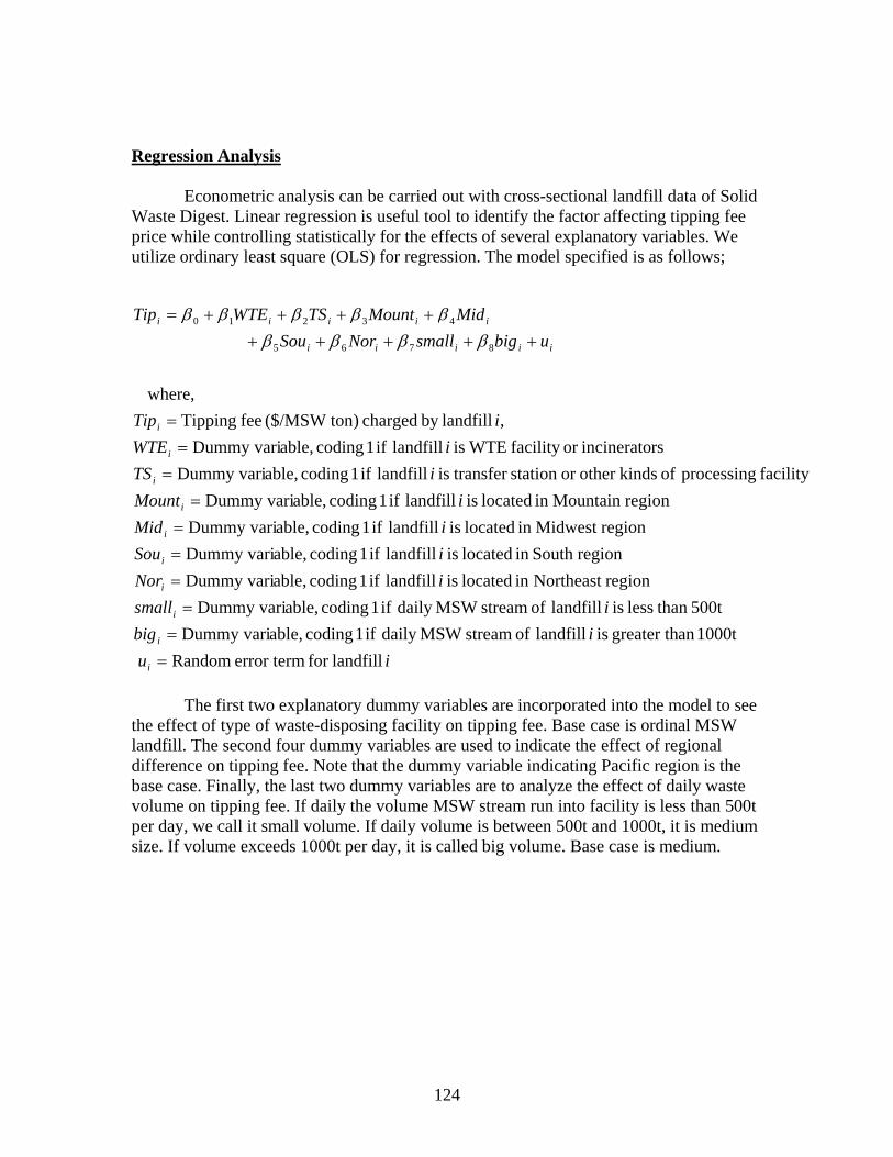
124
Regression Analysis
Econometric analysis can be carried out with cross-sectional landfill data of Solid Waste Digest. Linear regression is useful tool to identify the factor affecting tipping fee price while controlling statistically for the effects of several explanatory variables. We utilize ordinary least square (OLS) for regression. The model specified is as follows;
iuibig
ismalliNoriSouiMid
iMountiTS
iWTEiTip
ubigsmallNorSouMidMountTSWTETip
i
i
i
i
i
i
i
i
i
i
iiiii
iiiii
landfillfor error term Random 1000tan greater th is landfill of streamMSW daily if 1 coding able,Dummy vari
500t than less is landfill of streamMSW daily if 1 coding able,Dummy variregionNortheast in located is landfill if 1 coding able,Dummy vari
regionSouth in located is landfill if 1 coding able,Dummy variregionMidwest in located is landfill if 1 coding able,Dummy vari
regionMountain in located is landfill if 1 coding able,Dummy varifacility processing of kindsother or station transfer is landfill if 1 coding able,Dummy vari
rsincineratoor facility WTEis landfill if 1 coding able,Dummy vari, landfillby charged )($/MSW ton fee Tipping
where,
8765
43210
==
====
==
==
+++++++++=
βββββββββ
The first two explanatory dummy variables are incorporated into the model to see the effect of type of waste-disposing facility on tipping fee. Base case is ordinal MSW landfill. The second four dummy variables are used to indicate the effect of regional difference on tipping fee. Note that the dummy variable indicating Pacific region is the base case. Finally, the last two dummy variables are to analyze the effect of daily waste volume on tipping fee. If daily the volume MSW stream run into facility is less than 500t per day, we call it small volume. If daily volume is between 500t and 1000t, it is medium size. If volume exceeds 1000t per day, it is called big volume. Base case is medium.

125
Table A.3 OLS Regression Results
Variable Coefficient Std. Error t-statistics p-valueWTE 17.332 2.369 7.316 0.000TS 6.148 1.625 3.783 0.000
Mountain -18.892 2.489 -7.590 0.000Midwest -10.544 2.135 -4.938 0.000
South -8.512 2.111 -4.032 0.000Northeast 14.219 2.213 6.425 0.000
small_volume -1.772 3.595 -0.493 0.622large_volume 0.133 1.326 0.100 0.920
Intercept 39.828 1.983 20.086 0.000 N=745, R-square=0.37
The regression results reported in Table appendix 4.3 show that both type of facilities and regions have significant effects on tipping fee. Both WTE and TS charges higher tipping fee than ordinary MSW dumping landfill. F-statistics of these two dummy variables is 30.18 (p-value is 0.00), thus there is strong statistical evidence that tipping fee varies by type of facilities. F-statistics of regional four dummy variables is 68.61. Regional dummy variables are proxy to “population density indicators” or “landfill scarcity indicators”. For instance, Northeast region is heavily populated and has scarce landfill site, while in Mountain regions, population is scattered and landfill sites are abundant.
On the other hand, daily MSW volume shows no statistical relation with tipping fee. F-statistics of two dummy variables is only 0.14 (p-value is 0.87). In conclusion, tipping fee is not dependent on facility size but more affected by regional effect and type of facility.

126
APPENDIX B Table B.1 MSW Generation, Recycling, Landfilled by State in the U.S. in 200342 MSW
generated (1000t)
Population MSW per
capita (ton)
MSW recycled (1000t)
MSW to WTE (1000t)
MSW landfilled(1000t)
MSW recycled
(%)
MSW to WTE (%)
MSW landfilled
(%)
Number of MSW landfill
Number of WTE plants
Landfill capacity (1000t)
Capacity / landfilled
(year)
ImportedMSW
(1000t)
ExportedMSW
(1000t) West 38% 3% 59% Alaska n/a 643,786 n/a n/a n/a n/a n/a n/a n/a n/a n/a n/a n/a n/a n/aCalifornia 54,430 35,116,033 1.550 21,902 887 31,640 40.2% 1.6% 58.1% 161 3 410,501 8 26 616Hawaii 1,706 1,244,898 1.370 430 417 859 25.2% 24.4% 50.4% 9 1 n/a n/a n/a n/aNevada 3,366 2,173,491 1.548 532 0 2,834 15.8% 0.0% 84.2% 23 0 60,742 18 534 0Oregon 4,735 3,521,515 1.345 1,987 201 2,547 42.0% 4.3% 53.8% 30 1 n/a n/a 1,626 19
Washington 8,667 6,068,996 1.428 2,960 489 5,218 34.1% 5.6% 60.2% 21 4 180,003 21 173 1,146Mountain 9% 1% 90% Arizona 6,012 5,456,453 1.102 1,053 0 4,959 17.5% 0.0% 82.5% 41 0 n/a n/a 383 10Colorado 5,051 4,506,542 1.121 142 0 4,909 2.8% 0.0% 97.2% 65 0 n/a n/a n/a n/aIdaho 1,090 1,341,131 0.813 92 0 998 8.4% 0.0% 91.6% 29 0 n/a n/a n/a n/aMontana n/a 909,453 n/a n/a n/a n/a n/a n/a n/a 30 0 32,727 n/a n/a n/aNew Mexico 2,095 1,855,059 1.129 135 0 1,960 6.5% 0.0% 93.5% 35 0 190,966 91 378 0Utah 2,471 2,316,256 1.067 118 120 2,234 4.8% 4.9% 90.4% 38 1 n/a n/a 139 n/a
Wyoming 694 498,703 1.391 12 0 682 1.7% 0.0% 98.3% 53 0 n/a n/a n/a n/aMidwest 25% <1% 75% Arkansas 3,838 2,710,079 1.416 1,392 56 2,390 36.3% 1.5% 62.3% 24 2 n/a n/a 168 370Iowa 3,416 2,936,760 1.163 1,426 34 1,956 41.7% 1.0% 57.3% 59 1 40,183 12 403 128Kansas 4,698 2,715,884 1.730 540 0 4,158 11.5% 0.0% 88.5% 51 0 n/a n/a 663 n/aMissouri 7,257 5,672,579 1.279 2,823 20 4,413 38.9% 0.3% 60.8% 24 0 41,433 6 11 1,993Nebraska 2,395 1,729,180 1.385 369 0 2,026 15.4% 0.0% 84.6% 24 0 n/a n/a n/a n/aNorth Dakota 639 634,110 1.007 60 0 579 9.4% 0.0% 90.6% 14 0 n/a n/a 101 10Okalahoma 4,489 3,493,714 1.285 45 0 4,444 1.0% 0.0% 99.0% 40 1 n/a n/a n/a n/aSouth Dakota 518 761,063 0.681 15 0 503 3.0% 0.0% 97.0% 15 0 16,758 32 n/a n/a
Texas 28,532 21,779,893 1.310 7,107 0 21,425 24.9% 0.0% 75.1% 175 2 970,000 34 66 n/aGreat Lakes 27% 5% 68% Illinois 15,951 12,600,620 1.266 5,191 0 10,760 32.5% 0.0% 67.5% 51 0 212,394 13 5,801 n/aIndiana 9,542 6,159,068 1.549 3,340 648 5,555 35.0% 6.8% 58.2% 35 1 52,232 5 1,574 n/aMichigan 16,916 10,050,446 1.683 2,550 1,183 13,182 15.1% 7.0% 77.9% 52 4 143,939 9 3,831 n/aMinnesota 5,044 5,019,720 1.005 2,301 1,266 1,477 45.6% 25.1% 29.3% 21 15 18,700 4 n/a 636Ohio 16,211 11,421,267 1.419 3,808 0 12,403 23.5% 0.0% 76.5% 44 0 124,080 8 1,978 987
Wisconsin 5,593 5,441,196 1.028 1,378 188 4,027 24.6% 3.4% 72.0% 42 2 30,440 5 1,407 n/a
42 Data of Oregon and Maryland was corrected by BioCycle itself three months after “The State of Garbage in America” for 2003 is issued. Data of Oregon and Maryland is taken from “Corrections to State of Garbage of Garbage” (BioCycle 2004).

127
South 19% 12% 69% Alabama n/a 4,486,508 n/a n/a n/a n/a n/a n/a n/a n/a n/a n/a n/a n/a n/aFlorida 19,707 16,713,149 1.179 4,722 5,564 9,421 24.0% 28.2% 47.8% 100 13 n/a n/a n/a n/aGeorgia 11,214 8,560,310 1.310 929 52 10,234 8.3% 0.5% 91.3% 60 1 135,349 12 963 n/aKentucky 5,466 4,092,891 1.335 625 2 4,838 11.4% 0.0% 88.5% 25 1 36,364 7 n/a 247Louisiana 4,953 4,482,646 1.105 402 0 4,551 8.1% 0.0% 91.9% 24 0 n/a n/a n/a n/aMississippi 2,918 2,871,782 1.016 10 0 2,908 0.3% 0.0% 99.7% 17 0 n/a n/a 538 n/aNorth Carolina
8,981 8,320,146 1.079 992 121 7,869 11.0% 1.3% 87.6% 41 1 100,000 11 n/a 882
South Carolina
5,973 4,107,183 1.454 1,698 231 4,044 28.4% 3.9% 67.7% 19 4 109,534 18 955 508
Tennessee 7,366 5,797,289 1.271 1,943 150 5,273 26.4% 2.0% 71.6% 34 1 n/a n/a n/a 549
Virginia 10,878 7,293,542 1.491 3,161 2,152 5,565 29.1% 19.8% 51.2% 67 5 251,810 23 4,509 n/aMid Atlantic 28% 14% 58% Delaware 1,069 807,385 1.324 218 0 851 20.4% 0.0% 79.6% 3 0 20,000 19 n/a n/aMaryland 7,103 5,458,137 1.301 2,456 1,376 3,270 34.6% 19.4% 46.0% 20 3 n/a n/a 457 1,943New Jersey 10,606 8,590,300 1.235 4,015 962 5,630 37.9% 9.1% 53.1% 12 5 40,000 4 576 3,500New York 24,775 19,157,532 1.293 7,384 4,248 13,143 29.8% 17.1% 53.1% 26 10 90,000 4 568 5,400Pennsylvania 12,676 12,335,091 1.028 3,399 2,095 7,182 26.8% 16.5% 56.7% 49 6 298,586 24 10,000 3,000
West Virginia 1,755 1,801,873 0.974 120 0 1,634 6.9% 0.0% 93.1% 18 0 5,674 3 204 432New England 27% 34% 39% Connecticut 4,734 3,460,503 1.368 888 2,130 1,716 18.8% 45.0% 36.2% 2 6 n/a n/a 64 366Maine 1,327 1,294,464 1.025 650 448 229 49.0% 33.8% 17.2% 8 4 3,030 2 219 78Massachusetts 8,307 6,427,801 1.292 2,584 3,128 2,596 31.1% 37.6% 31.3% 19 7 n/a n/a 186 1,687New Hampshire
1,215 1,275,056 0.953 288 206 721 23.7% 17.0% 59.4% 10 2 15,000 12 746 33
Rhode Island 1,249 1,069,725 1.167 160 0 1,089 12.8% 0.0% 87.2% 2 0 n/a n/a n/a n/a
Vermont 612 616,592 0.992 183 56 373 29.8% 9.2% 60.9% 5 0 1,454 2 7 124United States 368,240 287,797,800 1.310 98,675 28,480 242,227 26.7% 7.7% 65.6% 1,767
Source: Kaufman et al., 2004

128
Figure B.1 Distribution of the U.S. Population in 2000 Source: U.S. Census Bureau, 2002

129
Figure B.2 Distribution of MSW in the U.S. in 2000 Source: County population data taken by U.S. Census Bureau (2002). State average MSW generation data taken by Goldstein and Madtes (2001)

130
Table B.2 MSW Density of Top 20 U.S. Populated Metropolitan Area
Metropolitan Area Population (million)
Area (square mile)
Population density (tons/
square mile)
State average MSW
generation (tons/year)
State average MSW
generation (lbs/day)
Annual MSW
generation (1000 tons
/year)
Daily MSW generation (1000 tons
/day)
MSW density
(tons/square mile
MSW within 10
radius (tons/100π square mile)
Minimum radius
supplying 500 TPD
(mile) New York--Northern New Jersey--Long Island 21.200 10,166 2,085 1.293 7.1 27,411 75.10 7.39 2,321 4.64 Los Angeles--Riverside--Orange County 16.374 33,966 482 1.550 8.5 25,379 69.53 2.05 643 8.82 Chicago--Gary--Kenosha 9.158 6,931 1,321 1.266 6.9 11,593 31.76 4.58 1,440 5.89 Washington--Baltimore 7.608 9,578 794 1.301 7.1 9,898 27.12 2.83 889 7.50 San Francisco--Oakland--San Jose 7.039 7,369 955 1.550 8.5 10,911 29.89 4.06 1,274 6.26 Philadelphia--Wilmington--Atlantic City 6.188 5,936 1,043 1.028 5.6 6,362 17.43 2.94 922 7.36 Boston--Worcester--Lawrence 5.819 6,450 902 1.292 7.1 7,518 20.60 3.19 1,003 7.06 Detroit--Ann Arbor--Flint 5.456 6,566 831 1.683 9.2 9,183 25.16 3.83 1,204 6.44 Dallas--Fort Worth 5.222 9,105 574 1.310 7.2 6,841 18.74 2.06 647 8.79 Houston--Galveston--Brazoria 4.670 7,707 606 1.310 7.2 6,117 16.76 2.17 683 8.55 Atlanta 4.112 6,126 671 1.310 7.2 5,387 14.76 2.41 757 8.13 Miami--Fort Lauderdale 3.876 3,154 1,229 1.179 6.5 4,570 12.52 3.97 1,247 6.33 Seattle--Tacoma--Bremerton 3.555 7,224 492 1.428 7.8 5,076 13.91 1.93 605 9.09 Phoenix--Mesa 3.252 14,574 223 1.102 6.0 3,584 9.82 0.67 212 15.37 Minneapolis--St. Paul 2.969 6,064 490 1.005 5.5 2,984 8.17 1.35 423 10.87 Cleveland--Akron 2.946 3,613 815 1.419 7.8 4,180 11.45 3.17 996 7.09 San Diego 2.814 4,205 669 1.550 8.5 4,361 11.95 2.84 893 7.48 St. Louis 2.604 6,393 407 1.279 7.0 3,330 9.12 1.43 448 10.56 Denver--Boulder--Greeley 2.582 8,496 304 1.121 6.1 2,894 7.93 0.93 293 13.06 Tampa--St. Petersburg--Clearwater 2.450 2,555 959 1.179 6.5 2,889 7.91 3.10 973 7.17
Data: Metropolitan population and area data is taken by U.S. Census Bureau. State average MSW generation data is taken by Kaufman et al. (2001)

131
APPENDIX C
Figure C.1 Cellulose Conversion by GPV Source: GeneSyst, 2004

132
APPENDIX D Table D.1 Revenue Schedule of a 500 TPD MSW-Ethanol Plant at the Base Case (U.S. Thousands Dollar)
Recovered material sales Chemical By-product sales Year
MSW volume (T/day)
MSW volume (T/year)
Ethanol sales Aluminum
sales Ferrous
sales Plastic sales
Furfural sales
Yeast sales
Gypsum sales
CO2 sales
Total revenue
0 0 0 0 0 0 - 0 0 0 0 0 1 500 156,000 5,070 983 262 - 390 346 9 117 7,177 2 510 159,120 5,171 1,002 267 - 796 706 9 119 8,072 3 520 162,302 5,275 1,023 273 - 812 721 9 122 8,233 4 531 165,548 5,380 1,043 278 - 828 735 9 124 8,398 5 541 168,859 5,488 1,064 284 - 844 750 10 127 8,566 6 552 172,237 5,598 1,085 289 - 861 765 10 129 8,737 7 563 175,681 5,710 1,107 295 - 878 780 10 132 8,912 8 574 179,195 5,824 1,129 301 - 896 796 10 134 9,090 9 586 182,779 5,940 1,152 307 - 914 812 10 137 9,272
10 598 186,434 6,059 1,175 313 - 932 828 11 140 9,457 11 609 190,163 6,180 1,198 319 - 951 844 11 143 9,646 12 622 193,966 6,304 1,222 326 - 970 861 11 145 9,839 13 634 197,846 6,430 1,246 332 - 989 878 11 148 10,036 14 647 201,803 6,559 1,271 339 - 1,009 896 11 151 10,237 15 660 205,839 6,690 1,297 346 - 1,029 914 12 154 10,441 16 673 209,955 6,824 1,323 353 - 1,050 932 12 157 10,650 17 686 214,155 6,960 1,349 360 - 1,071 951 12 161 10,863 18 700 218,438 7,099 1,376 367 - 1,092 970 12 164 11,081 19 714 222,806 7,241 1,404 374 - 1,114 989 13 167 11,302 20 728 227,263 7,386 1,432 382 - 1,136 1,009 13 170 11,528

133
Table D.2 Cost Schedule of a 500 TPD MSW-Ethanol Plant at the Base Case (U.S. Thousands Dollar) Total operation cost General Administration Overhead
Year MSW
volume (T/day)
MSW volume (T/year)
Capital Cost
Feedstock cost
MSW Classification
cost
Plant operation
cost
Admini-stration
cost
Insurance cost
Loyalty cost
Contractual cost
Training cost
Total cost
0 0 0 (30,000) 0 0 0 0 0 0 0 0 (30,000)1 500 156,000 0 5,054 (600) (1,794) (246) (80) (367) (50) (150) 1,767 2 510 159,120 0 5,155 (612) (1,830) (246) (80) (397) (75) (50) 1,866 3 520 162,302 0 5,259 (624) (1,866) (246) (80) (405) (100) (50) 1,887 4 531 165,548 0 5,364 (637) (1,904) (246) (80) (413) (125) (50) 1,909 5 541 168,859 (402) 5,471 (649) (1,942) (246) (80) (421) (150) (50) 1,531 6 552 172,237 0 5,580 (662) (1,981) (246) (80) (430) (175) (50) 1,957 7 563 175,681 0 5,692 (676) (2,020) (246) (80) (438) (200) (50) 1,982 8 574 179,195 0 5,806 (689) (2,061) (246) (80) (447) (225) (50) 2,008 9 586 182,779 0 5,922 (703) (2,102) (246) (80) (456) (250) (50) 2,035
10 598 186,434 (704) 6,040 (717) (2,144) (246) (80) (465) (275) (50) 1,360 11 609 190,163 0 6,161 (731) (2,187) (246) (80) (474) (300) (50) 2,093 12 622 193,966 0 6,285 (746) (2,231) (246) (80) (484) (325) (50) 2,123 13 634 197,846 0 6,410 (761) (2,275) (246) (80) (493) (350) (50) 2,155 14 647 201,803 0 6,538 (776) (2,321) (246) (80) (503) (375) (50) 2,187 15 660 205,839 (402) 6,669 (792) (2,367) (246) (80) (513) (400) (50) 1,819 16 673 209,955 0 6,803 (808) (2,414) (246) (80) (524) (425) (50) 2,256 17 686 214,155 0 6,939 (824) (2,463) (246) (80) (534) (450) (50) 2,292 18 700 218,438 0 7,077 (840) (2,512) (246) (80) (545) (475) (50) 2,329 19 714 222,806 0 7,219 (857) (2,562) (246) (80) (556) (500) (50) 2,368 20 728 227,263 0 7,363 (874) (2,614) (246) (80) (567) (525) (50) 2,408

134
Table D.3 Cash Flow of a 500 TPD MSW-Ethanol Plant under Different Tax Program Scenario (U.S. Thousands Dollar)
Debt Schedule Tax description Scenario 1 =No tax incentive
Scenario 2 =Tax program ends in Year 2
Scenario 3 = Tax program lasts by Year 15
T Year EBITDA Annual depreci-
ation Interest payment
Principal payment
Remaining Principal
Federal tax (32%)
State tax
(8.5%)
Local Tax
($50,000 a year)
Tax imposed
Cash flow
Tax imposed
Cash flow
Tax imposed
Cash flow
0 2005 (30,000) 0 0 0 (30,000) 0 0 0 0 (30,000) 0 (30,000) 0 (30,000)1 2006 8,944 (1,634) (2,100) (732) (29,268) (1,668) (443) (50) (2,160) 6,784 (493) 8,452 (493) 8,452 2 2007 9,937 (1,634) (2,049) (783) (28,485) (2,002) (532) (50) (2,583) 7,354 (582) 9,356 (582) 9,356 3 2008 10,120 (1,634) (1,994) (838) (27,647) (2,078) (552) (50) (2,680) 7,441 (2,680) 7,441 (602) 9,518 4 2009 10,307 (1,634) (1,935) (896) (26,751) (2,156) (573) (50) (2,779) 7,528 (2,779) 7,528 (623) 9,684 5 2010 10,096 (1,634) (1,873) (959) (25,792) (2,237) (594) (50) (2,882) 7,214 (2,882) 7,214 (644) 9,452 6 2011 10,694 (1,634) (1,805) (1,026) (24,765) (2,322) (617) (50) (2,988) 7,706 (2,988) 7,706 (667) 10,027 7 2012 10,894 (1,634) (1,734) (1,098) (23,667) (2,408) (640) (50) (3,098) 7,795 (3,098) 7,795 (690) 10,204 8 2013 11,098 (1,634) (1,657) (1,175) (22,492) (2,499) (664) (50) (3,212) 7,886 (3,212) 7,886 (714) 10,384 9 2014 11,307 (1,634) (1,574) (1,257) (21,235) (2,592) (688) (50) (3,330) 7,977 (3,330) 7,977 (738) 10,569
10 2015 10,817 (1,634) (1,486) (1,345) (19,889) (2,688) (714) (50) (3,452) 7,365 (3,452) 7,365 (764) 10,053 11 2016 11,739 (1,374) (1,392) (1,440) (18,450) (2,871) (763) (50) (3,684) 8,055 (3,684) 8,055 (813) 10,926 12 2017 11,962 (1,374) (1,291) (1,540) (16,909) (2,975) (790) (50) (3,815) 8,147 (3,815) 8,147 (857) 11,105 13 2018 12,191 (1,374) (1,184) (1,648) (15,261) (3,083) (819) (50) (3,952) 8,239 (3,952) 8,239 (934) 11,256 14 2019 12,424 (1,374) (1,068) (1,763) (13,498) (3,194) (848) (50) (4,093) 8,331 (4,093) 8,331 (1,015) 11,409 15 2020 12,260 (1,374) (945) (1,887) (11,611) (3,310) (879) (50) (4,239) 8,021 (4,239) 8,021 (1,100) 11,160 16 2021 12,906 (1,374) (813) (2,019) (9,592) (3,430) (911) (50) (4,392) 8,515 (4,392) 8,515 (4,392) 8,515 17 2022 13,155 (1,374) (671) (2,160) (7,432) (3,555) (944) (50) (4,550) 8,606 (4,550) 8,606 (4,550) 8,606 18 2023 13,410 (1,374) (520) (2,312) (5,120) (3,685) (979) (50) (4,714) 8,696 (4,714) 8,696 (4,714) 8,696 19 2024 13,670 (1,374) (358) (2,473) (2,647) (3,820) (1,015) (50) (4,885) 8,785 (4,885) 8,785 (4,885) 8,785 20 2025 13,936 (1,374) (185) (2,647) 0 (3,961) (1,052) (50) (5,063) 8,873 (5,063) 8,873 (5,063) 8,873
33.4% IRR = 24.5% IRR = 26.8% IRR = 31.4% 87,474 NPV = 52,291 NPV = 55,597 NPV = 74,072 10.4 B/C = 2.2 B/C = 2.4 B/C = 4.3

135
Table D.4 IRR Sensitivity with Changing Ethanol Price and Tipping Fee (EBITDA) Ethanol price ($/gallon) ±10% change
-100% -90% -80% -70% -60% -50% -40% -30% -20% -10% 0% 10% 20% 30% 40% 50% 60% 70% 80% 90% 100%
0.00 0.13 0.26 0.39 0.52 0.65 0.78 0.91 1.04 1.17 1.30 1.43 1.56 1.69 1.82 1.95 2.08 2.21 2.34 2.47 2.60 -100% 0.00 - - -4.5% -0.3% 3.0% 5.7% 8.1% 10.3% 12.4% 14.4% 16.3% 18.1% 19.9% 21.7% 23.4% 25.1% 26.8% 28.5% 30.2% 31.8% 33.5%-90% 3.60 - -4.6% -0.3% 3.0% 5.7% 8.1% 10.3% 12.4% 14.4% 16.3% 18.1% 19.9% 21.7% 23.4% 25.1% 26.8% 28.5% 30.2% 31.8% 33.5% 35.1%-80% 7.20 -4.6% -0.3% 2.9% 5.7% 8.1% 10.3% 12.4% 14.4% 16.3% 18.1% 19.9% 21.7% 23.4% 25.1% 26.8% 28.5% 30.2% 31.8% 33.5% 35.1% 36.8%-70% 10.80 -0.3% 2.9% 5.7% 8.1% 10.3% 12.4% 14.3% 16.2% 18.1% 19.9% 21.7% 23.4% 25.1% 26.8% 28.5% 30.2% 31.8% 33.5% 35.1% 36.8% 38.4%-60% 14.40 2.9% 5.7% 8.1% 10.3% 12.4% 14.3% 16.2% 18.1% 19.9% 21.6% 23.4% 25.1% 26.8% 28.5% 30.2% 31.8% 33.5% 35.1% 36.8% 38.4% 40.1%-50% 18.00 5.6% 8.1% 10.3% 12.4% 14.3% 16.2% 18.1% 19.9% 21.6% 23.4% 25.1% 26.8% 28.5% 30.2% 31.8% 33.5% 35.1% 36.8% 38.4% 40.1% 41.7%-40% 21.60 8.1% 10.3% 12.4% 14.3% 16.2% 18.1% 19.9% 21.6% 23.4% 25.1% 26.8% 28.5% 30.1% 31.8% 33.5% 35.1% 36.8% 38.4% 40.0% 41.7% 43.3%-30% 25.20 10.3% 12.3% 14.3% 16.2% 18.1% 19.9% 21.6% 23.4% 25.1% 26.8% 28.5% 30.1% 31.8% 33.5% 35.1% 36.8% 38.4% 40.0% 41.7% 43.3% 44.9%-20% 28.80 12.3% 14.3% 16.2% 18.1% 19.9% 21.6% 23.4% 25.1% 26.8% 28.5% 30.1% 31.8% 33.5% 35.1% 36.8% 38.4% 40.0% 41.7% 43.3% 44.9% 46.6%-10% 32.40 14.3% 16.2% 18.1% 19.9% 21.6% 23.4% 25.1% 26.8% 28.5% 30.1% 31.8% 33.5% 35.1% 36.7% 38.4% 40.0% 41.7% 43.3% 44.9% 46.6% 48.2%0% 36.00 16.2% 18.1% 19.9% 21.6% 23.4% 25.1% 26.8% 28.5% 30.1% 31.8% 33.4% 35.1% 36.7% 38.4% 40.0% 41.7% 43.3% 44.9% 46.6% 48.2% 49.8%10% 39.60 18.0% 19.8% 21.6% 23.3% 25.1% 26.8% 28.4% 30.1% 31.8% 33.4% 35.1% 36.7% 38.4% 40.0% 41.7% 43.3% 44.9% 46.6% 48.2% 49.8% 51.4%20% 43.20 19.8% 21.6% 23.3% 25.1% 26.8% 28.4% 30.1% 31.8% 33.4% 35.1% 36.7% 38.4% 40.0% 41.7% 43.3% 44.9% 46.6% 48.2% 49.8% 51.4% 53.1%30% 46.80 21.6% 23.3% 25.1% 26.8% 28.4% 30.1% 31.8% 33.4% 35.1% 36.7% 38.4% 40.0% 41.6% 43.3% 44.9% 46.5% 48.2% 49.8% 51.4% 53.1% 54.7%40% 50.40 23.3% 25.0% 26.7% 28.4% 30.1% 31.8% 33.4% 35.1% 36.7% 38.4% 40.0% 41.6% 43.3% 44.9% 46.5% 48.2% 49.8% 51.4% 53.1% 54.7% 56.3%50% 54.00 25.0% 26.7% 28.4% 30.1% 31.8% 33.4% 35.1% 36.7% 38.4% 40.0% 41.6% 43.3% 44.9% 46.5% 48.2% 49.8% 51.4% 53.1% 54.7% 56.3% 57.9%60% 57.60 26.7% 28.4% 30.1% 31.8% 33.4% 35.1% 36.7% 38.4% 40.0% 41.6% 43.3% 44.9% 46.5% 48.2% 49.8% 51.4% 53.1% 54.7% 56.3% 57.9% 59.6%70% 61.20 28.4% 30.1% 31.8% 33.4% 35.1% 36.7% 38.4% 40.0% 41.6% 43.3% 44.9% 46.5% 48.2% 49.8% 51.4% 53.0% 54.7% 56.3% 57.9% 59.6% 61.2%80% 64.80 30.1% 31.7% 33.4% 35.1% 36.7% 38.3% 40.0% 41.6% 43.3% 44.9% 46.5% 48.2% 49.8% 51.4% 53.0% 54.7% 56.3% 57.9% 59.6% 61.2% 62.8%90% 68.40 31.7% 33.4% 35.1% 36.7% 38.3% 40.0% 41.6% 43.3% 44.9% 46.5% 48.1% 49.8% 51.4% 53.0% 54.7% 56.3% 57.9% 59.6% 61.2% 62.8% 64.4%
Tipp
ing
fee
(%/to
n) ±
10%
cha
nge
100% 72.00 33.4% 35.0% 36.7% 38.3% 40.0% 41.6% 43.2% 44.9% 46.5% 48.1% 49.8% 51.4% 53.0% 54.7% 56.3% 57.9% 59.5% 61.2% 62.8% 64.4% 66.1%

136
Table D.5 IRR Sensitivity with Changing Ethanol Price and Tipping Fee (After Tax; No Tax Incentive case)
Ethanol price ($/gallon) ±10% change -100% -90% -80% -70% -60% -50% -40% -30% -20% -10% 0% 10% 20% 30% 40% 50% 60% 70% 80% 90% 100% 0.00 0.13 0.26 0.39 0.52 0.65 0.78 0.91 1.04 1.17 1.30 1.43 1.56 1.69 1.82 1.95 2.08 2.21 2.34 2.47 2.60
-100% 0.0 - - - - - - - - - -2.2% 2.1% 5.3% 8.1% 10.5% 12.8% 14.9% 17.0% 18.9% 20.8% 22.7% 24.6%-90% 3.6 - - - - - - - - -2.2% 2.1% 5.3% 8.1% 10.5% 12.8% 14.9% 17.0% 18.9% 20.8% 22.7% 24.5% 26.4%-80% 7.2 - - - - - - - -2.2% 2.0% 5.3% 8.0% 10.5% 12.8% 14.9% 17.0% 18.9% 20.8% 22.7% 24.5% 26.4% 28.1%-70% 10.8 - - - - - - -2.2% 2.0% 5.3% 8.0% 10.5% 12.8% 14.9% 16.9% 18.9% 20.8% 22.7% 24.5% 26.3% 28.1% 29.9%-60% 14.4 - - - - - -2.3% 2.0% 5.3% 8.0% 10.5% 12.8% 14.9% 16.9% 18.9% 20.8% 22.7% 24.5% 26.3% 28.1% 29.9% 31.7%-50% 18.0 - - - - -2.3% 2.0% 5.3% 8.0% 10.5% 12.8% 14.9% 16.9% 18.9% 20.8% 22.7% 24.5% 26.3% 28.1% 29.9% 31.7% 33.4%-40% 21.6 - - - -2.3% 2.0% 5.3% 8.0% 10.5% 12.8% 14.9% 16.9% 18.9% 20.8% 22.7% 24.5% 26.3% 28.1% 29.9% 31.7% 33.4% 35.1%-30% 25.2 - - -2.3% 2.0% 5.2% 8.0% 10.5% 12.7% 14.9% 16.9% 18.9% 20.8% 22.7% 24.5% 26.3% 28.1% 29.9% 31.6% 33.4% 35.1% 36.9%-20% 28.8 - -2.3% 2.0% 5.2% 8.0% 10.5% 12.7% 14.9% 16.9% 18.9% 20.8% 22.7% 24.5% 26.3% 28.1% 29.9% 31.6% 33.4% 35.1% 36.9% 38.6%-10% 32.4 -2.3% 2.0% 5.2% 8.0% 10.5% 12.7% 14.9% 16.9% 18.9% 20.8% 22.7% 24.5% 26.3% 28.1% 29.9% 31.6% 33.4% 35.1% 36.8% 38.6% 40.3%0% 36.0 2.0% 5.2% 8.0% 10.5% 12.7% 14.9% 16.9% 18.9% 20.8% 22.7% 24.5% 26.3% 28.1% 29.9% 31.6% 33.4% 35.1% 36.8% 38.6% 40.3% 42.0%10% 39.6 5.2% 8.0% 10.4% 12.7% 14.9% 16.9% 18.9% 20.8% 22.7% 24.5% 26.3% 28.1% 29.9% 31.6% 33.4% 35.1% 36.8% 38.6% 40.3% 42.0% 43.7%20% 43.2 8.0% 10.4% 12.7% 14.9% 16.9% 18.9% 20.8% 22.6% 24.5% 26.3% 28.1% 29.9% 31.6% 33.4% 35.1% 36.8% 38.6% 40.3% 42.0% 43.7% 45.4%30% 46.8 10.4% 12.7% 14.8% 16.9% 18.9% 20.8% 22.6% 24.5% 26.3% 28.1% 29.9% 31.6% 33.4% 35.1% 36.8% 38.6% 40.3% 42.0% 43.7% 45.4% 47.1%40% 50.4 12.7% 14.8% 16.9% 18.9% 20.8% 22.6% 24.5% 26.3% 28.1% 29.8% 31.6% 33.4% 35.1% 36.8% 38.5% 40.3% 42.0% 43.7% 45.4% 47.1% 48.8%50% 54.0 14.8% 16.9% 18.8% 20.8% 22.6% 24.5% 26.3% 28.1% 29.8% 31.6% 33.3% 35.1% 36.8% 38.5% 40.3% 42.0% 43.7% 45.4% 47.1% 48.8% 50.5%60% 57.6 16.9% 18.8% 20.8% 22.6% 24.5% 26.3% 28.1% 29.8% 31.6% 33.3% 35.1% 36.8% 38.5% 40.3% 42.0% 43.7% 45.4% 47.1% 48.8% 50.5% 52.2%70% 61.2 18.8% 20.7% 22.6% 24.5% 26.3% 28.1% 29.8% 31.6% 33.3% 35.1% 36.8% 38.5% 40.2% 42.0% 43.7% 45.4% 47.1% 48.8% 50.5% 52.2% 53.9%80% 64.8 20.7% 22.6% 24.5% 26.3% 28.1% 29.8% 31.6% 33.3% 35.1% 36.8% 38.5% 40.2% 42.0% 43.7% 45.4% 47.1% 48.8% 50.5% 52.2% 53.9% 55.6%90% 68.4 22.6% 24.4% 26.3% 28.0% 29.8% 31.6% 33.3% 35.1% 36.8% 38.5% 40.2% 42.0% 43.7% 45.4% 47.1% 48.8% 50.5% 52.2% 53.9% 55.6% 57.3%
Tipp
ing
fee
(%/to
n) ±
10%
cha
nge
100% 72.0 24.4% 26.3% 28.0% 29.8% 31.6% 33.3% 35.1% 36.8% 38.5% 40.2% 41.9% 43.7% 45.4% 47.1% 48.8% 50.5% 52.2% 53.9% 55.6% 57.3% 59.0%

137
Table D.6 IRR Sensitivity with Changing Ethanol Price and Tipping Fee (After Tax; Tax Incentives Ends in Year 15)
Ethanol price ($/gallon) ±10% change -100% -90% -80% -70% -60% -50% -40% -30% -20% -10% 0% 10% 20% 30% 40% 50% 60% 70% 80% 90% 100%
0.00 0.13 0.26 0.39 0.52 0.65 0.78 0.91 1.04 1.17 1.30 1.43 1.56 1.69 1.82 1.95 2.08 2.21 2.34 2.47 2.60 -100% 0.0 - - - - - - -3.3% 3.0% 6.7% 9.6% 12.1% 14.4% 16.5% 18.5% 20.5% 22.4% 24.3% 26.1% 27.9% 29.7% 31.4%
-90% 3.6 - - - - - -3.3% 3.0% 6.6% 9.5% 12.1% 14.4% 16.5% 18.5% 20.5% 22.4% 24.3% 26.1% 27.9% 29.6% 31.4% 33.1%-80% 7.2 - - - - -3.4% 3.0% 6.6% 9.5% 12.1% 14.4% 16.5% 18.5% 20.5% 22.4% 24.3% 26.1% 27.9% 29.6% 31.4% 33.1% 34.9%-70% 10.8 - - - -3.4% 3.0% 6.6% 9.5% 12.1% 14.3% 16.5% 18.5% 20.5% 22.4% 24.2% 26.1% 27.9% 29.6% 31.4% 33.1% 34.9% 36.6%-60% 14.4 - - -3.4% 2.9% 6.6% 9.5% 12.0% 14.3% 16.5% 18.5% 20.5% 22.4% 24.2% 26.1% 27.9% 29.6% 31.4% 33.1% 34.9% 36.6% 38.3%-50% 18.0 - -3.5% 2.9% 6.6% 9.5% 12.0% 14.3% 16.5% 18.5% 20.5% 22.4% 24.2% 26.1% 27.9% 29.6% 31.4% 33.1% 34.9% 36.6% 38.3% 40.0%-40% 21.6 -3.5% 2.9% 6.6% 9.5% 12.0% 14.3% 16.5% 18.5% 20.5% 22.4% 24.2% 26.1% 27.8% 29.6% 31.4% 33.1% 34.8% 36.6% 38.3% 40.0% 41.7%-30% 25.2 2.9% 6.6% 9.5% 12.0% 14.3% 16.5% 18.5% 20.5% 22.4% 24.2% 26.0% 27.8% 29.6% 31.4% 33.1% 34.8% 36.6% 38.3% 40.0% 41.7% 43.4%-20% 28.8 6.6% 9.5% 12.0% 14.3% 16.5% 18.5% 20.5% 22.4% 24.2% 26.0% 27.8% 29.6% 31.4% 33.1% 34.8% 36.6% 38.3% 40.0% 41.7% 43.4% 45.1%-10% 32.4 9.5% 12.0% 14.3% 16.5% 18.5% 20.5% 22.4% 24.2% 26.0% 27.8% 29.6% 31.4% 33.1% 34.8% 36.6% 38.3% 40.0% 41.7% 43.4% 45.1% 46.8%
0% 36.0 12.0% 14.3% 16.4% 18.5% 20.4% 22.4% 24.2% 26.0% 27.8% 29.6% 31.4% 33.1% 34.8% 36.5% 38.3% 40.0% 41.7% 43.4% 45.1% 46.8% 48.4%10% 39.6 14.3% 16.4% 18.5% 20.4% 22.3% 24.2% 26.0% 27.8% 29.6% 31.3% 33.1% 34.8% 36.5% 38.3% 40.0% 41.7% 43.4% 45.1% 46.8% 48.4% 50.1%20% 43.2 16.4% 18.5% 20.4% 22.3% 24.2% 26.0% 27.8% 29.6% 31.3% 33.1% 34.8% 36.5% 38.2% 40.0% 41.7% 43.4% 45.1% 46.7% 48.4% 50.1% 51.8%30% 46.8 18.5% 20.4% 22.3% 24.2% 26.0% 27.8% 29.6% 31.3% 33.1% 34.8% 36.5% 38.2% 40.0% 41.7% 43.4% 45.0% 46.7% 48.4% 50.1% 51.8% 53.5%40% 50.4 20.4% 22.3% 24.2% 26.0% 27.8% 29.6% 31.3% 33.1% 34.8% 36.5% 38.2% 39.9% 41.6% 43.3% 45.0% 46.7% 48.4% 50.1% 51.8% 53.5% 55.2%50% 54.0 22.3% 24.2% 26.0% 27.8% 29.6% 31.3% 33.1% 34.8% 36.5% 38.2% 39.9% 41.6% 43.3% 45.0% 46.7% 48.4% 50.1% 51.8% 53.5% 55.2% 56.9%60% 57.6 24.2% 26.0% 27.8% 29.6% 31.3% 33.1% 34.8% 36.5% 38.2% 39.9% 41.6% 43.3% 45.0% 46.7% 48.4% 50.1% 51.8% 53.5% 55.2% 56.8% 58.5%70% 61.2 26.0% 27.8% 29.6% 31.3% 33.1% 34.8% 36.5% 38.2% 39.9% 41.6% 43.3% 45.0% 46.7% 48.4% 50.1% 51.8% 53.5% 55.2% 56.8% 58.5% 60.2%80% 64.8 27.8% 29.6% 31.3% 33.1% 34.8% 36.5% 38.2% 39.9% 41.6% 43.3% 45.0% 46.7% 48.4% 50.1% 51.8% 53.5% 55.2% 56.8% 58.5% 60.2% 61.9%90% 68.4 29.5% 31.3% 33.0% 34.8% 36.5% 38.2% 39.9% 41.6% 43.3% 45.0% 46.7% 48.4% 50.1% 51.8% 53.5% 55.1% 56.8% 58.5% 60.2% 61.9% 63.6%
Tipp
ing
fee
($/to
n)±1
0%ch
ange
100% 72.0 31.3% 33.0% 34.8% 36.5% 38.2% 39.9% 41.6% 43.3% 45.0% 46.7% 48.4% 50.1% 51.8% 53.5% 55.1% 56.8% 58.5% 60.2% 61.9% 63.6% 65.2%

138
Table D.7 NPV Sensitivity with Changing Ethanol Price and Tipping Fee (EBITDA; U.S. Million Dollar) Ethanol price ($/gallon) ±10% change
-100% -90% -80% -70% -60% -50% -40% -30% -20% -10% 0% 10% 20% 30% 40% 50% 60% 70% 80% 90% 100%
0.00 0.13 0.26 0.39 0.52 0.65 0.78 0.91 1.04 1.17 1.30 1.43 1.56 1.69 1.82 1.95 2.08 2.21 2.34 2.47 2.60-100% 0.0 (33.52) (27.46) (21.40) (15.34) (9.28) (3.22) 2.84 8.90 14.95 21.01 27.07 33.13 39.19 45.25 51.31 57.37 63.43 69.48 75.54 81.60 87.66
-90% 3.6 (27.48) (21.42) (15.36) (9.30) (3.24) 2.82 8.88 14.94 20.99 27.05 33.11 39.17 45.23 51.29 57.35 63.41 69.47 75.52 81.58 87.64 93.70 -80% 7.2 (21.44) (15.38) (9.32) (3.26) 2.80 8.86 14.92 20.98 27.03 33.09 39.15 45.21 51.27 57.33 63.39 69.45 75.51 81.56 87.62 93.68 99.74 -70% 10.8 (15.40) (9.34) (3.28) 2.78 8.84 14.90 20.96 27.02 33.08 39.13 45.19 51.25 57.31 63.37 69.43 75.49 81.55 87.60 93.66 99.72 105.78-60% 14.4 (9.36) (3.30) 2.76 8.82 14.88 20.94 27.00 33.06 39.12 45.17 51.23 57.29 63.35 69.41 75.47 81.53 87.59 93.65 99.70 105.76 111.82-50% 18.0 (3.32) 2.74 8.80 14.86 20.92 26.98 33.04 39.10 45.16 51.21 57.27 63.33 69.39 75.45 81.51 87.57 93.63 99.69 105.74 111.80 117.86-40% 21.6 2.72 8.78 14.84 20.90 26.96 33.02 39.08 45.14 51.20 57.25 63.31 69.37 75.43 81.49 87.55 93.61 99.67 105.73 111.78 117.84 123.90-30% 25.2 8.76 14.82 20.88 26.94 33.00 39.06 45.12 51.18 57.24 63.29 69.35 75.41 81.47 87.53 93.59 99.65 105.71 111.77 117.82 123.88 129.94-20% 28.8 14.81 20.86 26.92 32.98 39.04 45.10 51.16 57.22 63.28 69.34 75.39 81.45 87.51 93.57 99.63 105.69 111.75 117.81 123.87 129.92 135.98-10% 32.4 20.85 26.90 32.96 39.02 45.08 51.14 57.20 63.26 69.32 75.38 81.43 87.49 93.55 99.61 105.67 111.73 117.79 123.85 129.91 135.96 142.02
0% 36.0 26.89 32.94 39.00 45.06 51.12 57.18 63.24 69.30 75.36 81.42 87.47 93.53 99.59 105.65 111.71 117.77 123.83 129.89 135.95 142.00 148.0610% 39.6 32.93 38.98 45.04 51.10 57.16 63.22 69.28 75.34 81.40 87.46 93.51 99.57 105.63 111.69 117.75 123.81 129.87 135.93 141.99 148.04 154.1020% 43.2 38.97 45.02 51.08 57.14 63.20 69.26 75.32 81.38 87.44 93.50 99.55 105.61 111.67 117.73 123.79 129.85 135.91 141.97 148.03 154.08 160.1430% 46.8 45.01 51.07 57.12 63.18 69.24 75.30 81.36 87.42 93.48 99.54 105.60 111.65 117.71 123.77 129.83 135.89 141.95 148.01 154.07 160.13 166.1840% 50.4 51.05 57.11 63.16 69.22 75.28 81.34 87.40 93.46 99.52 105.58 111.64 117.69 123.75 129.81 135.87 141.93 147.99 154.05 160.11 166.17 172.2250% 54.0 57.09 63.15 69.20 75.26 81.32 87.38 93.44 99.50 105.56 111.62 117.68 123.73 129.79 135.85 141.91 147.97 154.03 160.09 166.15 172.21 178.2660% 57.6 63.13 69.19 75.24 81.30 87.36 93.42 99.48 105.54 111.60 117.66 123.72 129.77 135.83 141.89 147.95 154.01 160.07 166.13 172.19 178.25 184.3070% 61.2 69.17 75.23 81.29 87.34 93.40 99.46 105.52 111.58 117.64 123.70 129.76 135.81 141.87 147.93 153.99 160.05 166.11 172.17 178.23 184.29 190.3480% 64.8 75.21 81.27 87.33 93.38 99.44 105.50 111.56 117.62 123.68 129.74 135.80 141.86 147.91 153.97 160.03 166.09 172.15 178.21 184.27 190.33 196.3990% 68.4 81.25 87.31 93.37 99.42 105.48 111.54 117.60 123.66 129.72 135.78 141.84 147.90 153.95 160.01 166.07 172.13 178.19 184.25 190.31 196.37 202.43
Tipp
ing
fee
($/to
n) ±
10%
cha
nge
100% 72.0 87.29 93.35 99.41 105.46 111.52 117.58 123.64 129.70 135.76 141.82 147.88 153.94 159.99 166.05 172.11 178.17 184.23 190.29 196.35 202.41 208.47

139
Table D.8 NPV Sensitivity with Changing Ethanol Price and Tipping Fee (Scenario 1; U.S. Million Dollar) Ethanol price ($/gallon) ±10% change
-100% -90% -80% -70% -60% -50% -40% -30% -20% -10% 0% 10% 20% 30% 40% 50% 60% 70% 80% 90% 100%
0.00 0.13 0.39 0.52 0.65 0.78 0.91 1.04 1.17 1.30 1.43 1.56 1.69 1.82 1.95 2.08 2.21 2.34 2.47 2.60
-100% 0.0 (72.44) (66.20) (59.95) (53.70) (47.46) (41.21) (34.96) (28.72) (22.47) (16.23) (9.98) (3.73) 2.51 8.76 15.01 21.25 27.50 33.74 39.99 46.24 52.48 -90% 3.6 (66.22) (59.97) (53.72) (47.48) (41.23) (34.98) (28.74) (22.49) (16.25) (10.00) (3.75) 2.49 8.74 14.99 21.23 27.48 33.72 39.97 46.22 52.46 58.71 -80% 7.2 (59.99) (53.74) (47.50) (41.25) (35.00) (28.76) (22.51) (16.26) (10.02) (3.77) 2.47 8.72 14.97 21.21 27.46 33.71 39.95 46.20 52.44 58.69 64.94 -70% 10.8 (53.76) (47.52) (41.27) (35.02) (28.78) (22.53) (16.28) (10.04) (3.79) 2.46 8.70 14.95 21.19 27.44 33.69 39.93 46.18 52.43 58.67 64.92 71.16 -60% 14.4 (47.53) (41.29) (35.04) (28.80) (22.55) (16.30) (10.06) (3.81) 2.44 8.68 14.93 21.17 27.42 33.67 39.91 46.16 52.41 58.65 64.90 71.14 77.39 -50% 18.0 (41.31) (35.06) (28.81) (22.57) (16.32) (10.08) (3.83) 2.42 8.66 14.91 21.16 27.40 33.65 39.89 46.14 52.39 58.63 64.88 71.13 77.37 83.62 -40% 21.6 (35.08) (28.83) (22.59) (16.34) (10.10) (3.85) 2.40 8.64 14.89 21.14 27.38 33.63 39.87 46.12 52.37 58.61 64.86 71.11 77.35 83.60 89.85 -30% 25.2 (28.85) (22.61) (16.36) (10.11) (3.87) 2.38 8.62 14.87 21.12 27.36 33.61 39.86 46.10 52.35 58.59 64.84 71.09 77.33 83.58 89.83 96.07 -20% 28.8 (22.63) (16.38) (10.13) (3.89) 2.36 8.61 14.85 21.10 27.34 33.59 39.84 46.08 52.33 58.58 64.82 71.07 77.31 83.56 89.81 96.05 102.30-10% 32.4 (16.40) (10.15) (3.91) 2.34 8.59 14.83 21.08 27.32 33.57 39.82 46.06 52.31 58.56 64.80 71.05 77.29 83.54 89.79 96.03 102.28 108.530% 36.0 (10.17) (3.93) 2.32 8.57 14.81 21.06 27.31 33.55 39.80 46.04 52.29 58.54 64.78 71.03 77.28 83.52 89.77 96.01 102.26 108.51 114.7510% 39.6 (3.94) 2.30 8.55 14.79 21.04 27.29 33.53 39.78 46.03 52.27 58.52 64.76 71.01 77.26 83.50 89.75 96.00 102.24 108.49 114.73 120.9820% 43.2 2.28 8.53 14.77 21.02 27.27 33.51 39.76 46.01 52.25 58.50 64.74 70.99 77.24 83.48 89.73 95.98 102.22 108.47 114.71 120.96 127.2130% 46.8 8.51 14.76 21.00 27.25 33.49 39.74 45.99 52.23 58.48 64.73 70.97 77.22 83.46 89.71 95.96 102.20 108.45 114.70 120.94 127.19 133.4340% 50.4 14.74 20.98 27.23 33.47 39.72 45.97 52.21 58.46 64.71 70.95 77.20 83.45 89.69 95.94 102.18 108.43 114.68 120.92 127.17 133.42 139.6650% 54.0 20.96 27.21 33.46 39.70 45.95 52.19 58.44 64.69 70.93 77.18 83.43 89.67 95.92 102.16 108.41 114.66 120.90 127.15 133.40 139.64 145.8960% 57.6 27.19 33.44 39.68 45.93 52.18 58.42 64.67 70.91 77.16 83.41 89.65 95.90 102.15 108.39 114.64 120.88 127.13 133.38 139.62 145.87 152.1270% 61.2 33.42 39.66 45.91 52.16 58.40 64.65 70.89 77.14 83.39 89.63 95.88 102.13 108.37 114.62 120.87 127.11 133.36 139.60 145.85 152.10 158.3480% 64.8 39.64 45.89 52.14 58.38 64.63 70.88 77.12 83.37 89.61 95.86 102.11 108.35 114.60 120.85 127.09 133.34 139.58 145.83 152.08 158.32 164.5790% 68.4 45.87 52.12 58.36 64.61 70.86 77.10 83.35 89.60 95.84 102.09 108.33 114.58 120.83 127.07 133.32 139.57 145.81 152.06 158.30 164.55 170.80
Tipp
ing
fee
($/to
n) ±
10%
cha
nge
100% 72.0 52.10 58.34 64.59 70.84 77.08 83.33 89.58 95.82 102.07 108.31 114.56 120.81 127.05 133.30 139.55 145.79 152.04 158.29 164.53 170.78 177.02

140
Table D.9 NPV Sensitivity with Changing Ethanol Price and Tipping Fee (Scenario 3; U.S. Million Dollar) Ethanol price ($/gallon) ±10% change
-100% -90% -80% -70% -60% -50% -40% -30% -20% -10% 0% 10% 20% 30% 40% 50% 60% 70% 80% 90% 100% 0.00 0.13 0.26 0.39 0.52 0.65 0.78 0.91 1.04 1.17 1.30 1.43 1.56 1.69 1.82 1.95 2.08 2.21 2.34 2.47 2.60
-100% 0.0 (50.66) (44.42) (38.17) (31.92) (25.68) (19.43) (13.18) (6.94) (0.69) 5.55 11.80 18.05 24.29 30.54 36.79 43.03 49.28 55.53 61.77 68.02 74.26 -90% 3.6 (44.43) (38.19) (31.94) (25.70) (19.45) (13.20) (6.96) (0.71) 5.54 11.78 18.03 24.27 30.52 36.77 43.01 49.26 55.51 61.75 68.00 74.24 80.49 -80% 7.2 (38.21) (31.96) (25.71) (19.47) (13.22) (6.98) (0.73) 5.52 11.76 18.01 24.26 30.50 36.75 42.99 49.24 55.49 61.73 67.98 74.23 80.47 86.72 -70% 10.8 (31.98) (25.73) (19.49) (13.24) (7.00) (0.75) 5.50 11.74 17.99 24.24 30.48 36.73 42.97 49.22 55.47 61.71 67.96 74.21 80.45 86.70 92.95 -60% 14.4 (25.75) (19.51) (13.26) (7.01) (0.77) 5.48 11.72 17.97 24.22 30.46 36.71 42.96 49.20 55.45 61.69 67.94 74.19 80.43 86.68 92.93 99.17 -50% 18.0 (19.53) (13.28) (7.03) (0.79) 5.46 11.71 17.95 24.20 30.44 36.69 42.94 49.18 55.43 61.68 67.92 74.17 80.41 86.66 92.91 99.15 105.40-40% 21.6 (13.30) (7.05) (0.81) 5.44 11.69 17.93 24.18 30.42 36.67 42.92 49.16 55.41 61.66 67.90 74.15 80.39 86.64 92.89 99.13 105.38 111.63-30% 25.2 (7.07) (0.83) 5.42 11.67 17.91 24.16 30.41 36.65 42.90 49.14 55.39 61.64 67.88 74.13 80.38 86.62 92.87 99.11 105.36 111.61 117.85-20% 28.8 (0.85) 5.40 11.65 17.89 24.14 30.39 36.63 42.88 49.13 55.37 61.62 67.86 74.11 80.36 86.60 92.85 99.10 105.34 111.59 117.83 124.08-10% 32.4 5.38 11.63 17.87 24.12 30.37 36.61 42.86 49.11 55.35 61.60 67.84 74.09 80.34 86.58 92.83 99.08 105.32 111.57 117.81 124.06 130.310% 36.0 11.61 17.86 24.10 30.35 36.59 42.84 49.09 55.33 61.58 67.83 74.07 80.32 86.56 92.81 99.06 105.30 111.55 117.80 124.04 130.29 136.5310% 39.6 17.84 24.08 30.33 36.57 42.82 49.07 55.31 61.56 67.81 74.05 80.30 86.55 92.79 99.04 105.28 111.53 117.78 124.02 130.27 136.52 142.7620% 43.2 24.06 30.31 36.56 42.80 49.05 55.29 61.54 67.79 74.03 80.28 86.53 92.77 99.02 105.26 111.51 117.76 124.00 130.25 136.50 142.74 148.9930% 46.8 30.29 36.54 42.78 49.03 55.28 61.52 67.77 74.01 80.26 86.51 92.75 99.00 105.25 111.49 117.74 123.98 130.23 136.48 142.72 148.97 155.2240% 50.4 36.52 42.76 49.01 55.26 61.50 67.75 73.99 80.24 86.49 92.73 98.98 105.23 111.47 117.72 123.97 130.21 136.46 142.70 148.95 155.20 161.4450% 54.0 42.74 48.99 55.24 61.48 67.73 73.98 80.22 86.47 92.71 98.96 105.21 111.45 117.70 123.95 130.19 136.44 142.68 148.93 155.18 161.42 167.6760% 57.6 48.97 55.22 61.46 67.71 73.96 80.20 86.45 92.70 98.94 105.19 111.43 117.68 123.93 130.17 136.42 142.67 148.91 155.16 161.40 167.65 173.9070% 61.2 55.20 61.44 67.69 73.94 80.18 86.43 92.68 98.92 105.17 111.41 117.66 123.91 130.15 136.40 142.65 148.89 155.14 161.39 167.63 173.88 180.1280% 64.8 61.43 67.67 73.92 80.16 86.41 92.66 98.90 105.15 111.40 117.64 123.89 130.13 136.38 142.63 148.87 155.12 161.37 167.61 173.86 180.10 186.3590% 68.4 67.65 73.90 80.15 86.39 92.64 98.88 105.13 111.38 117.62 123.87 130.12 136.36 142.61 148.85 155.10 161.35 167.59 173.84 180.09 186.33 192.58
Tipp
ing
fee
($/to
n) ±
10%
cha
nge
100% 72.0 73.88 80.13 86.37 92.62 98.86 105.11 111.36 117.60 123.85 130.10 136.34 142.59 148.83 155.08 161.33 167.57 173.82 180.07 186.31 192.56 198.80

141
Figure D.1 Effect of Furfural Price on IRR
Figure D.2 Effect of Aluminum Price on IRR
0%
5%
10%
15%
20%
25%
30%
35%
0 200 400 600 800 1000
Aluminum Price ($/ton)
IRR
Scenario 1 Scenario 2 Scenario 3
0%
5%
10%
15%
20%
25%
30%
35%
0.00 0.10 0.20 0.30 0.40 0.50 0.60
Furfural Price ($/lbs)
IRR
Scenario 1 Scenario 2 Scenario 3

142
APPENDIX E
Table E.1 Time Line of MSW-Ethanol Project of PMO in the City of Middletown, NY
Source: Times Herald-Record 2004
Date Event
February 1994 Pencor, a Baltimore development agency, says it wants to build a recycling and manufacturing plant in Middletown.
December 1994 Pencor Orange Corp. proposes designing, building and operating a waste-ethanol facility in Middletown. The proposal is in reply to a city request for a company to handle its MSW.
January 1995 Pencor is named joins with Masada OxyNol Inc., a subsidiary of Masada Resource Group, to form Pencor-Masada OxyNol LLC. (PMO).
January 1996
The city’s Common Council gives then-city Public Works Commissioner authority to solicit trash from neighbors to make a plant viable. The goal is 700 TPD. Middletown generates 50 TPD. The promise of a long-term, fixed price on tipping fees is attractive to many communities.
September 1997 Middletown officially signs on to the project as a customer. Five other Orange County communities already are signed on to deliver their trash to PMO.
August 1998 Orange County lawmakers reject PMO’s offer to take county garbage.
March 1999 25 municipalities or garbage districts sign up to pay PMO to haul and process garbage. The city Planning Board approves PMO’s plan to build on a former city landfill.
December 1999 Nearly 500 people cram a public hearing on the PMO’s proposal. Many are concerned about the potential for the plant to pollute the city’s south end.
July 2001 Middletown asks Kroll Associates, an international risk management firm, to review PMO.
November 2001 Kroll requests documents from PMO. PMO provides some material but refuses or fails to turn over much of the requested information.
October 2002 After reading the Kroll report, the Common Council agrees to spend $50,000 to hire a Long Island law firm that specializes in complex contracts and limiting risk.
November 2003 The common Council receives a copy of the final draft of a contract between the city and PMO. Thy mayor says all questions raised by the Kroll report have been satisfied.
December 8th 2003 The Common Council votes on whether to authorize the mayor to sign a contract with PMO. Finally Mayor is allowed to make a contract with PMO.

143
BIBLIOGRAPHY
Abbott, Charles. "Update 2-Senate Approves 5 Bln Gallon U.S. Ethanol Mandate." Reuters, June 5 2003.
Ackerman, Frank. Why Do We Recycle: Markets, Values, and Public Policy. Washington
D.C.: Island Press, 1997. Ames, Jermy. "Chicago Bans MTBE." ECO (Ethanol Climate Protection Oil Reduction):
A Public Forum Issue XII, January 19 2001. Araman, Philip., Bush, Robert J., and Reddy, Vijay S. "Municipal Solid Waste Landfills
and Wood Pallets: What's Happening in the U.S." Pallet Enterprise 17, no. 2 (1997): 50-56.
ARI (Alternative Resource, Inc.). "Ethanol Facility Financial Feasibility Report."
Alternative Resource, Inc, 1999. Available from http://www.genesyst.com/Independent_Study/Ethanol Facility Financial Feasibility Report.pdf
Arkenol. Arkenol, Inc. Website [cited 2004]. Available from http://www.arkenol.com/. Badder, B.C. "Trucking Garbage to Ohio." MSW Management (1999). Badger, P.C. "Ethanol from Cellulose: A General Review." In Trends in New Crops and
New Uses, edited by Jules. Janick, and Whipkey, Anna. Alexandria, VA: ASHS Press, 2002.
BBI International Consulting Division. "Economic Impact Assessment for Ethanol
Production and Use in Hawaii." Final Report. Honolulu, 2003. Available from http://www.hawaii.gov/dbedt/ert/ewg/ethanol-bbi2.pdf
BioCycle. "Ethanol from Waste Paper." BioCycle 33, no. 8 (1992): 6. Boardman, Anthony E., Greenberg, David H., Vining, Aidan R., and Weimer, David L.
Cost-Benefit Analysis : Concepts and Practice. 2nd ed. Upper Saddle River, NJ: Prentice Hall Inc., 2001.
Brady, Patricia D., Hudak, Paul F., and Dickson, Kenneth L. "Surveying the Commercial
Municipal Solid Wastestream in Denton, Texas." MSW Management 10, no. 5 (2000).
144
Broder, Jacqueline D., Harris, Robbert A., and Ranney, Jeffrey T. "Using MSW and Industrial Residues as Ethanol Feedstock." BioCycle 42, no. 10 (2001): 23-26.
Broder, Jacqueline D., Wayne Barrier, J., and Bulls, M.M. "Producing Fuel Ethanol and
Other Chemicals Form Municipal Solid Waste." Paper presented at the 1991 International Summer Meeting of The American Society of Agricultural Engineers, Muscle Shoals, AL, June 1991.
Broder, Jacqueline D., Barrier, John W., Lambert, Rusell O., Millicent M. Bulls, Henson,
L Jack., Shipely, Tania M., Sheffey, Lenora L., Faucett, Lewis., and Eley, Michael H. 1993. Municipal Solid Waste and Waste Cellulosic Conversion to Fuels and Chemicals: April 1990 - September 1992. Muscle Shoals, Alabama: Tennessee Valley Authority, Biotechnical Research Department.
California Energy Commission. "U.S. Ethanol Industry Production Capacity Outlook."
2001a. Available from http://www.energy.ca.gov/reports/2001-08-29_600-01-017.PDF
———."Costs and Benefits of a Biomass-to-Ethanol Production Industry in California."
2001b. Available from http://www.energy.ca.gov/reports/2001-04-03_500-01-002+002A.PDF
Cascadia Consulting Group, Inc. "Wisconsin Statewide Waste Characterization Study."
2003. Available from http://www.dnr.state.wi.us/org/aw/wm/publications/recycle/wrws-finalrpt.pdf
Cascadia Consulting Group, Inc., and Sky Valley Associates. "2002 Residential Waste
Stream Composition Study." Seattle: Seattle Public Utility, 2003. CFDC (Clean Fuel Development Coalition). "CFDC Pricing Analysis Shows Ethanol
Prices Consistently Comparable to Gasoline." 2004. Available from http://www.cleanfuelsdc.org/issues/pricing_analysis.htm
Chartwell Information Publishers. "Year-End Data Review." Solid Waste Digest 13, no.
1-2 (2003): 1-36. Chemical Market Reporter. several years. City of Middletown. Web Site of City of Middle Town in Orange County in N.Y. [cited
2004]. Available from http://www.ci.middletown.ny.us/. Conrad, Jon M. Resource Economics. Cambridge, UK: Cambridge University Press,
1999.

145
Curlee, T Randall., Schexnayder, Susan M., Vogt, David P., Wolfe, Amy K., Kelsay, Michael P., and Feldmand, David L. Waste-to-Energy in the United States: A Social and Economic Assessment. Westport, CT: Quorum Books, 1994.
DAI (Downstream Alternatives, Inc). "Infrastructure Requirements for an Expanded
Ethanol Industry." South Bend, IN,: DAI, 2002. Dale, Bruce E. "Biomass Refining: Protein and Ethanol from Alfalfa." I&EC Research
and Development 22 (1983): 466. DiPardo, Joseph. "Outlook for Biomass Ethanol Production and Demand." Washington
D.C.: EIA, 2002. Available from http://www.eia.doe.gov/oiaf/analysispaper/pdf/biomass.pdf
DOE (U.S. Department of Energy). "Ethanol Milestones." Washington D.C.: U.S. DOE,
2003. Available from http://www.eia.doe.gov/cneaf/solar.renewables/renewable.energy.annual/backgrnd/chap8d.htm
———. "Biomass Program." Washington D.C.: U.S. DOE, Office of Energy Efficiency
and Renewable Energy, 2004. Available from http://www.eere.energy.gov/biomass/
Duff, S. "Interstate Waste Keeps Crossing the Lines." Waste News 5 (2001). Edelstein, Michael R. 2004. Sustainable Innovation and the Siting Dilemma; Thoughts on
the Stigmatization of Projects and Proponents, Good and Bad. Journal of Risk Research 7 (2):233-50.
EIA (Energy Information Administration). "Status and Impact of State MTBE Bans."
Washington D.C.: EIA, 2002a. Available from http://www.eia.doe.gov/oiaf/servicerpt/mtbeban/table1.html
———. "Alternatives to Traditional Transportation Fuels 2000." Washington D.C: EIA,
2002b. Available from http://www.eia.doe.gov/cneaf/alternate/page/datatables/atf1-13_00.html
———. "Review of Transportation Issues and Comparison of Infrastructure Costs for a
Renewable Fuels Standard." EIA: the Office of Integrated Analysis and Forecasting, 2002c. Available from http://tonto.eia.doe.gov/FTPROOT/service/question3.pdf
———. "The State Consumption Data." Washington D.C.: EIA, 2003. Available from
http://www.eia.doe.gov/emeu/states/_use_multistate.html

146
———. "Annual Energy Outlook 2004 with Projections to 2025." Washington D.C.: EIA, 2004a. Available from http://www.eia.doe.gov/oiaf/aeo/
———. "Monthly Oxygenate Telephone Report (Historical)." Washington D.C.: EIA,
2004b. Available from http://www.eia.doe.gov/oil_gas/petroleum/data_publications/monthly_oxygenate_telephone_report/motr_historical.html
Ezzet, L. "Solid Waste Services in the 100 Largest U.S. Cities." MSW Management
(1997). Farmdoc (Farm Design Outreach Central). 2004. Farmdoc website [cited 2004].
Available from http://www.farmdoc.uiuc.edu/index.html. Fehrs, Jeffrey PE. "Secondary Mill Residues and Urban Wood Waste Quantities in the
United States: Final Report." Washington D.C.: Northeast Regional Biomass Program, CONEG Policy Center, Inc., 1999. Available from http://www.nrbp.org/pdfs/pub21.pdf
Fox, Peter. Personal Communication. 2004. Fox, Peter., Fentes, Javier., and Bonger, Donald P. "Market Development Program for
Refuse to Alcohol Plants in Arizona." Final Report for Western Regional Biomass Energy Program (WRBEP). 1999. Available from http://www.westbioenergy.org/reports/55015/55015final.htm
Frazier Barnes & Associates, LLC. Ethanol Plant Map [cited 2004]. Available from
http://www.frazierbarnes.com/html/ethanol_plant_map.html. Galbe, M., and Zacchi, G. "A Review of the Production of Ethanol from Softwood." Appl
Microbbiol Biotechnol 59 (2002): 618-28. Gallagher, Paul W., Dikeman, Mark., Fritz, John., Wailes, Eric., Gauthier, Wayne., and
Shapouri, Hosein. "Supply and Social Cost Estimates for Biomass from Crop Residues in the United States." Environmental and Resource Economics 24, no. 4 (2003): 335-58.
GAO (U.S. General Accounting Office). "U.S. Ethanol Market: MTBE Ban in
California." Washington D.C.: U.S. GAO, 2002. Available from http://www.gao.gov/new.items/d02440r.pdf
GeneSyst International, Inc. Ethanol from Waste [cited 2004]. Available from
http://www.genesyst.com/Ethanol_from_Waste/Ethanol_From_Waste.htm. Glenn, Jim. "The State of Garbage in America." BioCycle 39, no. 4 (1998a): 32-43.

147
———. "The State of Garbage in America." BioCycle 39, no. 5 (1998b): 48-52. Goldstein, Nora. 2003. Solid Waste Composting Trends in the United States. BioCycle 44
(1):38-44. Goldstein, Nora., and Madtes, Celeste. "The State of Garbage in America." BioCycle 42,
no. 12 (2001): 42-53. Gray, Kevin. 1999. MSW and Biosolids become Feedstock for Ethanol. BioCycle 40
(8):37-38. Great Lakes Chemical Corporation. 1987. Great Lakes Chemical Corporation Annual
Report. Hadder, Jerry. "Estimation of Ethanol Demand in Gasoline." Oak Ridge National
Laboratory, 1997. Heimlich, Joe E. 2004. Community Household Hazardous Materials Programs [cited
2004]. Available from http://ohioline.osu.edu/cd-fact/0113.html. Hutzler, Mary. "Outlook for Transportation Fuel Supplies: 2003 and Beyond." Paper
presented at the 8th Annual National Ethanol Conference: Policy and Marketing, Scottsdale, Arizona 2003. Available from http://www.eia.doe.gov/oiaf/presentation/transportation/pdf/transportation.pdf
Jones, J.L., and Semrau, K.T. "Wood Hydrolysis for Ethanol Production: Previous
Experience and the Economics of Selected Processes." Biomass 5 (1984): 109-35. Kaufman, Scott M., Goldstein, Nora., Millrath, Karsten., and Themelis, Nickolas J. "The
State of Garbage in America." 45, no. 1 (2004): 31-41. Larson, S., Palmqvist, E., Hahn-Hagerdal, B., Tengborg, C., Stenberg, K., Zacchi, G., and
Nilverbrant, N.O. "The Generation of Fermentation Inhibitors During Dilute Acid Hydrolysis of Softwood." Enzyme Microb Technol 24 (1999): 151-59.
Levy, Joel., and Yokose, Kazuteru. 2004. CEH Report: Furfural. In Chemical Economics
Handbook, edited by SRI. Consulting. Mann, Michael D., and Bryan, Mike. "Feasibility of Producing Ethanol from Biomass in
Northeastern North Dakota and Northwestern Minnesota." Final Report prepared for Western Regional Biomass Energy Program (WRBEP). 2001. Available from http://www.westbioenergy.org/reports/mm-ethanol.htm
Masada. Masada Resource Group Website. 2004 [cited August 2004]. Available from
http://www.masada.com/.

148
Mcaloon, Andrew., Taylor, Frank., Yee, Winnie., Ibsen, Kelly., and Wooley, Robert. 2000. Determining the Cost of Producing Ethanol from Corn Starch and Lignocellulosic Feedstocks. Golden, Colorado: National Renewable Energy Laboratory (NREL). Available from http://www.nrel.gov/docs/fy01osti/28893.pdf
McCathy, J.E. "Interstate Shipment of Municipal Solid Waste: 1998 Update."
Congressional Research Service, 1998. Missouri Value Added Development Center. "Pumping Ethanol from the Farm to the
Vehicle: A Brief Look at the Industry." Value Added News to Agricultural Entrepreneurs, May 2001.
NESCAUM (North Eastern States For Coordinated Air Use Management). "Air Quality,
Fuel Supply and Cost Impacts of MTBE and Its Alternative." 1999. Pace, David. "Campaign Investments May Pay Off." Seacoast Newspapers, November 17
2003. Porter, Richard C. The Economics of Waste. Washington D.C.: Resource for The Future,
2002. Repa, Edward W. "Interstate Movement." Waste Age (1997). ———. "Solid Waste Disposal Trends." Waste Age 31, no. 4 (2000): 262-65. ———. "Tipping through Time." Waste Age 33, no. 11 (2002): 72. RFA (Renewable Fuel Association). "Ethanol Industry Outlook 2001: Clean Air, Clean
Water, Clean Fuel." Washington D.C.: RFA, 2001a. Available from http://www.ethanolrfa.org/rfareport2001.html?NS-search-set=\4029a\s49.29a845&NS-doc-offset=10&
———. "RFA Highlight Ethanol's Positive Impact on Jobs, Rural Economics at House
Small Business Subcommittee Hearing." RFA Member Press Releases, July 2001b.
Roberts, R.R., and Hilton, H.W. "Sugarcane Bagasse as a Potential Source of Ethanol and
Methanol Biofuels." Department of Business and Economic Development, State of Hawaii, 1988.
SENES Consultant, Limited. "Waste Paper as a Biomass Feedstock." Ottawa, Ontario,
Canada: Efficiency and Alternative Energy Technology Branch, CANMET, Natural Resources Canada, 1993.

149
Shapouri, Hosein., Gallagher, Paul., and Graboski, Michael S. 2002. USDA's 1998 U.S. Ethanol Cost-of-Production Survey. Washington D.C.: USDA (U.S. Department of Agriculture).
Solid Waste Management Coordinating Board. "Statewide MSW Composition Study: A
Study of Discards in the State of Minnesota." Final Report. 2000. Available from http://www.moea.state.mn.us/publications/wastesort2000.pdf
State of Hawaii, Department of Business, Economic Development & Tourism. "Ethanol
Production in Hawaii: Processes, Feedstock, and Current Economic Feasibility of Fuel Grade Ethanol Production in Hawaii." Final Report. Honolulu, 1994. Available from http://www.hawaii.gov/dbedt/ert/ethanol/ethanol94.pdf
State of Pennsylvania, Department of Environmental Protection. "Statewide Municipal
Waste Composition Study." 2003. Available from http://www.dep.state.pa.us/dep/deputate/airwaste/wm/recycle/waste_comp/study.htm
Tally, Steve. "Making Biofuel from Corn Stover." BioCycle 43, no. 11 (2002): 62. Technology and Management Services, Inc. "Information Regarding Ethanol Delivery
Infrastructure." Gaithersburg, MD, 2002. Themelis, Nickolas J. "Analyzing Data in State of Garbage in America, EPA Reports."
BioCycle 44, no. 1 (2003): 22-25. Themelis, Nickolas J., and Kaufman, Scott M. "State of Garbage in America: Data and
Methodology Assessment." BioCycle 45, no. 4 (2004): 22-26. Themelis, Nickolas J., Kim, Young Hwan., and Brady, Mark H. "Energy Recovery from
New York City Solid Wastes." Waste Management and Research 20 (2002): 223-33.
Tilton, Helga. "Chemical Prices." Chemical Market Reporter (various years) Titmas, James. Personal Communication. 2004. Time Herald-Record. Masada Project 2004 Available from http://www.recordonline.com/news/masada/masada.htm. University of Central Florida. MSW Learning Tool [cited 2004]. Available from
http://msw.cecs.ucf.edu/index.html. U.S. Bureau of the Census. "Ranking Tables for Metropolitan Areas: 1990 and 2000."
U.S. Census, Bureau, 2001. Available from http://www.census.gov/population/cen2000/phc-t3/tab03.pdf

150
U.S. Department of Labor, Bureau of Labor Statistics. 2004. Producer Price Index [cited
2004]. Available from http://www.bls.gov/ppi/home.htm. U.S. Department of Transportation. "Availability and Use of Alternative Fuels." 2002. U.S. EPA (Environmental Protection Agency). "Solid Waste Handbook." Washington
D.C.: U.S. EPA, 1997. ———. "Municipal Solid Waste in the United States: 2001 Figures and Facts."
Washington D.C.: U.S. EPA, 2003. Available from http://www.epa.gov/epaoswer/non-hw/muncpl/pubs/msw2001.pdf
———. "MTBE (Methyl Tertiary-Butyl Ether) and Underground Storage Tanks."
Washington D.C.: U.S. EPA, 2004a. Available from http://www.epa.gov/swerust1/mtbe/
———. "Reformulated Gasoline." Washington D.C.: 2004b. Available from
http://www.epa.gov/otaq/rfg.htm Walsh, Marie E., Perlack, Robert L., Turhollow, Anthony., Ugarte, Daniel de la Torre.,
Becker, Denny A., Graham, Robin L., Slinsky, Stephen E., and Ray, Daryll E. "Biomass Feedstock Availability in the United States: 1999 State Level Analysis." Oak Ridge, TN: Oak ridge National Laboratory, Oak ridge, TN., 2000.
Waste News for Chicago Market. several years. Whims, John. "Pipeline Consideration for Ethanol." Sparks Companies, Inc., 2002. Wooley, Robert., Ruth, Mark., Glassner, David., and Sheehan, John. "Process Design and
Costing of Bioethanol Technology: A Tool for Determining the Status and Direction of Research and Development." Biotechnology Progress 15, no. 5 (1999): 794-803.
Wyman, CE. 1996. Ethanol Production from Lignocellulosic Biomass: Overview. In
Handbook on Bioethanol: Production and Utilization, edited by C. Wyman. Bristol, PA: Taylor & Francis Group.
Yaency, Mark. Personal Communication. 2004.