the fields instrument suite on mms: scientific …...the fields instrument suite on mms 107 fig. 1...

Space Sci Rev (2016) 199:105–135DOI 10.1007/s11214-014-0109-8

The FIELDS Instrument Suite on MMS: ScientificObjectives, Measurements, and Data Products

R.B. Torbert · C.T. Russell · W. Magnes · R.E. Ergun · P.-A. Lindqvist · O. LeContel ·H. Vaith · J. Macri · S. Myers · D. Rau · J. Needell · B. King · M. Granoff ·M. Chutter · I. Dors · G. Olsson · Y.V. Khotyaintsev · A. Eriksson · C.A. Kletzing ·S. Bounds · B. Anderson · W. Baumjohann · M. Steller · K. Bromund · Guan Le ·R. Nakamura · R.J. Strangeway · H.K. Leinweber · S. Tucker · J. Westfall ·D. Fischer · F. Plaschke · J. Porter · K. LappalainenReceived: 14 May 2014 / Accepted: 16 October 2014 / Published online: 19 November 2014© The Author(s) 2014. This article is published with open access at Springerlink.com

R.B. Torbert (B) · O. LeContel · H. Vaith · J. Macri · S. Myers · D. Rau · J. Needell · B. King ·M. Granoff · M. Chutter · I. DorsUniversity of New Hampshire, Durham, NH, USAe-mail: [email protected]

G. OlssonRoyal Institute of Technology, Stockholm, Sweden

Y.V. Khotyaintsev · A. ErikssonSwedish Institute of Space Physics, Uppsala, Sweden

J. Porter · K. LappalainenUniversity of Oulu, Oulu, Finland

R.E. Ergun · S. Tucker · J. WestfallUniversity of Colorado, Boulder, CO, USA

R.B. TorbertSouthwest Research Institute, San Antonio, TX, USA

C.T. Russell · R.J. Strangeway · H.K. LeinweberUniversity of California, Los Angeles, CA, USA

K. Bromund · G. LeNASA Goddard Space Flight Center, Greenbelt, MD, USA

C.A. Kletzing · S. BoundsUniversity of Iowa, Iowa City, IA, USA

B. AndersonJohns Hopkins Applied Physics Laboratory, Laurel, MD, USA

W. Magnes · W. Baumjohann · M. Steller · R. Nakamura · D. Fischer · F. PlaschkeSpace Research Institute, Austrian Academy of Sciences, Graz, Austria

P.-A. LindqvistLaboratory for Plasma Physics, Paris, France

http://crossmark.crossref.org/dialog/?doi=10.1007/s11214-014-0109-8&domain=pdf

mailto:[email protected]

106 R.B. Torbert et al.

Abstract The FIELDS instrumentation suite on the Magnetospheric Multiscale (MMS)mission provides comprehensive measurements of the full vector magnetic and electric fieldsin the reconnection regions investigated by MMS, including the dayside magnetopause andthe night-side magnetotail acceleration regions out to 25 Re. Six sensors on each of the fourMMS spacecraft provide overlapping measurements of these fields with sensitive cross-calibrations both before and after launch. The FIELDS magnetic sensors consist of redun-dant flux-gate magnetometers (AFG and DFG) over the frequency range from DC to 64 Hz,a search coil magnetometer (SCM) providing AC measurements over the full whistler modespectrum expected to be seen on MMS, and an Electron Drift Instrument (EDI) that cali-brates offsets for the magnetometers. The FIELDS three-axis electric field measurementsare provided by two sets of biased double-probe sensors (SDP and ADP) operating in ahighly symmetric spacecraft environment to reduce significantly electrostatic errors. Thesesensors are complemented with the EDI electric measurements that are free from all lo-cal spacecraft perturbations. Cross-calibrated vector electric field measurements are thusproduced from DC to 100 kHz, well beyond the upper hybrid resonance whose frequencyprovides an accurate determination of the local electron density. Due to its very large geo-metric factor, EDI also provides very high time resolution (∼ 1 ms) ambient electron fluxmeasurements at a few selected energies near 1 keV. This paper provides an overview of theFIELDS suite, its science objectives and measurement requirements, and its performance asverified in calibration and cross-calibration procedures that result in anticipated errors lessthan 0.1 nT in B and 0.5 mV/m in E. Summaries of data products that result from FIELDSare also described, as well as algorithms for cross-calibration. Details of the design andperformance characteristics of AFG/DFG, SCM, ADP, SDP, and EDI are provided in fivecompanion papers.

Keywords Magnetic reconnection · Magnetospheric dynamics · Magnetosphericmultiscale · Electromagnetic field measurements

1 Introduction

The paradigm of magnetic reconnection has been one of the central organizing principles ofspace physics since it was first comprehensively used by Dungey (1953) to explain explosivespace plasma phenomena such as magnetic storms and solar flares, although suggestions ofthe principles of reconnection were put forward earlier by Giovanelli (1946), Hoyle (1949),and Cowling (1953). Theories of the process were put forward by Sweet and Parker (1957,1963) that led to the conclusion that conventional MHD processes were much too slow toaccommodate the explosive events that are attributed to reconnection. An alternative theoryby Petschek (1964) seemed to have resolved this issue with the inclusion of MHD shocks,which, however, were never conclusively observed in the extensive observations aroundthe Earth’s dayside magnetopause and magnetotail, regions where Dungey had suggestedreconnection must take place and which were accessible to in-situ measurement with space-craft. Nevertheless, an extensive body of observational evidence has been accumulated withspacecraft such as ISEE, AMPTE, Polar, Wind, Cluster and THEMIS that lead to the presentscientific consensus that reconnection is surely taking place in these regions, and other as-trophysical settings as well, but that no clear understanding of its underlying mechanism ismanifest. As of this writing, neither observations nor theory have enough fidelity to pinpointthis mechanism, or mechanisms.

The general picture that has remained valid since Dungey (at least for two-dimensionalreconnection where opposing magnetic fields are anti-parallel) is sketched in Fig. 1 (Mozer

The FIELDS Instrument Suite on MMS 107

Fig. 1 Two-dimensionalreconnection topology

et al. 2002). The anti-parallel primary magnetic field in the z direction is embedded in theplasma which flows with an E × B or “frozen in” velocity, and transports magnetic flux inopposing x directions under the influence of the reconnection electric field, in the y directionnormal to the page. This field is converted into mechanical energy that accelerates the plasmain jets of z-directed velocity with speeds of order the Alfvén speed of the incoming plasma.Observations have confirmed the suggestions of Sonnerup (1984) and others that a scaleseparation is established due to the different inertia of ions and electrons, whereby the ionsare accelerated and do not flow with a E × B velocity over a region of size di = c/ωpi

whereas the electrons remain frozen in until a much smaller scale region is encountered, ofsize c/ωpe. This separation is the effect of the Hall J × B term in the generalized Ohm’s lawfor plasmas:

E + U × B = ηJ + 1

enJ × B − 1

en∇ · ←→Pe + me

ne2

∂J∂t

(1)

where η is the resistivity (presumably anomalous, due to high frequency plasma waves) andPe is the electron pressure tensor. The Hall separation establishes a perpendicular electricfield, Ex , and a perturbation magnetic field, By , that results in an observed quadrupolarmagnetic signature on the scale size of the of ion diffusion region. However, the relativecontributions of the Hall term to those of others in Ohm’s law that give rise to dissipationand energy conversion, the inertial term, the pressure term, and the resistivity term (whichfor collisionless plasmas is mainly due to anomalous resistivity from wave action) is a matterof hot debate in both the observational and theoretical literature. In particular, the role of theelectric field parallel to the magnetic field, which cannot be driven by the Hall term, is notclear.

The observational situation can be exemplified by the data from the Cluster 4 spacecraftseen in Fig. 2 (Andre et al. 2004). These data are taken in a thin (∼ 20 km) current layer nearthe dayside magnetopause with the highest time resolution available to Cluster. This currentlayer exists on the magnetospheric side of the magnetopause and cannot be identified bythe authors as the electron diffusion region, although it is of the size of the electron inertiallength (4 km), but is probably the signature of a separatrix that extends from such a region.The layer can be seen in the magnetic field data of panel (e) and the estimated currents ofpanel (f), extending over approximately one second. There are 50 mV/m perpendicular elec-tric fields seen in panel (c), which agree with the estimate of the J × B term in Eq. (1), using


Fig. 2 Cluster encounter with thin reconnection current sheet

the currents in panel (f) estimated from the single satellite magnetic field profile (essentially,dB/(vdt)). Thus, this electric field may be predominately a Hall electric field. Panels (a) and(b) are spectra of electrons at velocities nearly perpendicular and parallel, respectively, tothe magnetic field. As the directions of these fluxes are changing as the satellite spins witha period of 4 seconds, a full distribution function cannot be determined for either electronsor ions, but the data in panels (b) and (f) indicate that a parallel current is present, carried by∼ 150 eV electrons.

The red line of panel (c) is a proxy for the pressure term of Eq. (1), and would suggest thatthis term is not important for this reconnection event. However, the full evaluation of thisterm is not possible with previous satellite instrumentation, including that for Cluster, and


Fig. 3 Simulation results for E parallel to B (Egedal et al. 2012)

this result is open to question. Cluster cannot determine the important parallel componentof the electric field, except in very rare current sheet orientations, because there were no3-axis sensors for this mission. The authors also confirm that the pressure terms and theinertial term, which would correspond to a parallel electric field, are impossible to determinefrom the time and energy resolution available with Cluster instrumentation, nor is theresufficient ion flux resolution to determine the U×B term in Ohm’s law on these time scales.Thus, although this observation hints at intriguing reconnection dynamics occurring on thescale size of the electron diffusion region, the important discriminating mechanisms for thereconnection process are undetermined.

Because satellites are capable of sampling only one or a few points (four, in the caseof Cluster and MMS), in-situ measurements have been supplemented with more and moresophisticated plasma simulations. In fact, MMS has a resident theory and modeling team(see Hesse et al. 2014, this issue) to provide models that are tailored to the experimentalconditions that MMS may experience. At this time, these simulations are limited in theirapproximations to the quite complex plasmas that surround reconnection regions, and thereare controversial and divergent opinions between various simulations as to the critical char-acteristics of reconnection. The example of the role of the parallel electric field serves toillustrate this situation.

Figure 3 shows the parallel electric field and an estimate of the potential along the fieldline from a simulation by Egedal et al. (2012). The authors claim that the significant ener-gization of electrons that has been observed in reconnection can be attributed to the parallelacceleration seen here all along the separatrix of the primary x-point (at ∼ 155di ), but thereis very little parallel field near that x-point. Pritchett and Mozer (2009) report a simulation(see Fig. 4) that also has no parallel signature right at the x-point, but closely surrounding itand with a different spatial distribution of the field. If the curl of the field is non-zero sur-rounding the diffusion region, it will contribute importantly to non-frozen-in electron flow,but the total electron energization may be significantly less than that seen in the simulationby Egedal. Nearly all discussions like these agree that the parallel electric field is a criti-cal parameter in reconnection, but may differ widely regarding both the contribution of thatfield and also the spatial characteristics of the field amplitude around diffusion regions. Forexample, Drake (2010) reports other simulations that attribute the electron energy gain toFermi-like acceleration between rapidly fluctuating magnetic islands. An accurate measure-ment of the parallel electric field is one of the major goals of the MMS FIELDS suite, as its


Fig. 4 Topologies of fields andrelated quantities for asymmetricreconnection with no guide field(Pritchett and Mozer 2009)

magnitude and distribution will discriminate among competing theories and simulations ofreconnection.

2 Science Objectives and Requirements

The importance of the reconnection process lies in the fact that it is the universal process bywhich magnetic energy is transferred to material particles in plasmas, as manifest in the so-lar wind’s interaction with the Earth’s magnetosphere, and in the explosive release of energyduring substorms, solar flares, and high-energy astrophysical events. To resolve the ques-tions remaining from previous missions and the extensive investigations of simulations ofreconnection, the MMS mission was charged with three primary objectives: (1) understandthe microphysics of magnetic reconnection by determining the kinetic processes occurringin the electron diffusion region that are responsible for collisionless magnetic reconnection,especially how reconnection is initiated; (2) determine the role played by electron inertialeffects and turbulent dissipation in driving magnetic reconnection in the electron diffusionregion; and (3) determine the rate of magnetic reconnection and the parameters that controlit. The FIELDS suite provides data that is critical to achieving these objectives. Specifically,the FIELDS suite must resolve thin currents layers and magnetic fields within reconnectionregions (and provide estimates of their gradients and curls with the use of multi-spacecraftobservations), detect and identify plasma wave modes and characteristics; measure the de-coupling of electrons from the magnetic field within the electron diffusion regions; deter-mine the agents for energization of energetic electrons and ions; measure the 3D componentsof the reconnection electric field and, particularly, its parallel component.

As the name “magnetic reconnection” implies, MMS studies of reconnection require theprecise measurement of the magnetic field, which is the source of the driving energy forreconnection. The magnetic field not only delineates the topology of connection and revealsthe presence of current sheets where energy conversion occurs and electromagnetic wavesthat might produce that conversion, it also illuminates the geometry for particle motion andacceleration. The FIELDS suite measures the magnetic field with four independent sensorsand provides algorithms for combining these four measurements into one precisely cali-brated time series up to 16000 samples/s, sufficient to determine the role of the whistlermode in the kinetic physics of reconnection. The electric field determines energy conver-sion and particle acceleration within reconnection regions, and combined with the magneticfields data, determines not only the frozen-in velocity, but also J · E and the waves that play


Fig. 5 Simulation results fornon-frozen flow condition

a role in turbulent dissipation. The FIELDS suite encompasses three measurements of theelectric field and again employs algorithms to combine these measurements to provide thefirst continuous, accurate determination of the 3D electric field. From this, the critical mea-surement of the parallel electric field can be deduced. Moreover, the magnetic and electricsignatures seen by the MMS fleet as a whole are critical in determining the location of eachof the satellites relative to reconnection structures such as those seen in Fig. 1.

The requirements on the electric and magnetic field sensors were determined by referenceto the unmet needs of previous experimental studies as referenced above and to a seriesof simulations of the diffusion regions that were guided by such studies. For example, asignature of reconnection dissipation is the presence of a parallel electric field and a parallelcurrent that are co-aligned (Jpar ·Epar > 0) relative to the local magnetic field. Given that theHall electric fields seen above were of order 50 to 100 mV/m, an angular error of 1 degreein the magnetic field direction, in diffusion regions where the magnitude of B may be 5–10nT, implies an accuracy of no better that 1 mV/m on the parallel electric field. This may bethe order of such a component in many places around reconnection sites. The one degreerequirement in turn implies an accuracy of ∼ 0.1 nT on each magnetic field component.For another perspective, Hesse (private communication) has simulated the terms in the lefthand side of Eq. (1) above to determine the magnitude of the reconnection electric fieldcomponent in the ion diffusion region, as seen in Fig. 5. To determine when E might besignificantly different from the −U × B, it is clear that an accuracy of order 1 mV/m isneeded.

These studies led to the following requirements on the FIELDS suite:

(1) measure the vector DC magnetic field with accuracy of 0.1 nT every 10 ms.(2) measure the vector (3D) DC electric field with accuracy better than 1 mV/m every 1 ms.(3) measure plasma waves (electric vector to 100 kHz, magnetic vector to 6 kHz).

The first two of these requirements have proven to be very challenging in previous spaceplasma missions. The FIELDS suite meets these challenges by combining multiple sensorsand multiple techniques that, in combination, are able to satisfy these demands.


3 Fields Suite Description

The above objectives are accomplished on MMS with six sensors integrated into the FIELDSsuite, as diagrammed in Fig. 6 (institutional contributions indicated), with the control anddata flow managed by the Central Electronics Box (CEB). The CEB also contains controllersfor the Analog Flux Gate (AFG), Digital Flux Gate (DFG), and the Electron Drift Instrument(EDI) as well as the Digital Signal Processor (DSP) for the high frequency instruments ofSearch Coil Magnetometer (SCM), Spin-plane Double-Probes (SDP), and the Axial Double-Probes (ADP). Within the CEB, the Central Data Processing Unit (CDPU) coordinates allthe functioning of the FIELDS suite, including power switching through the Low VoltagePower Supply (LVPS). The CDPU, LVPS, and DSP are all fully cold redundant. The CEBdetermines the synchronous timing regimen for the entire suite, all command processing,and can deliver up to 4 Mbps of data to the MMS spacecraft Central Instrument Data Pro-cessor (CIDP). Each of these sensors is described more completely in following companionpapers, but this communication attempts to describe how they are all integrated togetherinto one highly calibrated and cross-calibrated instrument suite to measure electromagneticfields more precisely and comprehensively than has ever been done in space before.

The sensors are arranged on each of the four MMS spacecraft according to Fig. 7.

3.1 Analog Flux-Gate and Digital Flux-Gate

The DC magnetometer measurements are provided by two flux-gate three-axis sensors, eachat the end of 5-meter deployable booms, and associated electronics within the CEB. Pro-vided by UCLA, each sensor consists of two magnetic cores, their housings and drive wirewindings, 6 sense wire windings, 6 feedback wire windings, and two printed circuit boardsmounted on an armature, which provides a framework for the components (see Russell et al.2014, this issue, for a more complete discussion). The Analog Flux-Gate (AFG) has a some-what different controller, provided also by UCLA, than the Digital Flux-Gate, which is

Fig. 6 FIELDS system configuration


Fig. 7 FIELDS sensors on a MMS spacecraft

provided by IWF, but both magnetometers evolved to basically the same digital feedbackdesign, although the DFG is implemented on a specially designed ASIC. Each controllerproduces a fixed 128 samples/s data stream to the Central Data Processing Unit (CDPU)within the CEB, which implements digital filters to reduce the sample rate if necessarydue to telemetry restrictions. Two output ranges are available for both AFG and DFG, of∼ 500 nT magnitude for low range to ∼ 8200/10500 nT (AFG/DFG), for high range. Theranges are commanded by the CDPU using an algorithm with hysteresis based on the datafrom the magnetometer controllers. Because of the key role of the magnetic field for re-connection studies, AFG and DFG provide fully redundant 3D data streams that are usedboth on-board the spacecraft by other instruments and also for ground processing. Exten-sive calibration and cross-calibration of the magnetometers was undertaken at the TechnicalUniversity Braunschweig. An extensive magnetic cleanliness program for the MMS satel-lite system was supervised and validated by the magnetometer team. Also, timing calibra-tions were performed to determine the phase and gain curves versus frequency, as shown inFigs. 16 and 17. These calibration data show that both the AFG and DFG have the capabilityto measure the DC and low frequency component of the vector magnetic field over the fullrange of each magnetometer with a timing accuracy of better than 0.1 ms.

In order to reach the science objectives, the AFG and DFG magnetometers are alsocalibrated on orbit. The calibration procedures include comparison of the AFG and DFGgains and offsets across range changes, Earth-field comparisons, cross-calibration with


Fig. 8 FM2 SCM transfer function (gain) in dBV/nT from 30 mHz to 50 kHz

EDI, and inter-spacecraft calibration. More information can be found in Russell et al.(2014, this issue).

3.2 Search Coil Magnetometer

The SCM provides the three components of the magnetic fluctuations in the 1 Hz–6 kHznominal frequency range, which is the imposed requirement. This range includes the hybridwave and kinetic Alfvén wave frequency range as well as whistler mode waves (up to theircut off frequency equal to the electron gyrofrequency) and solitary waves. SCM consists ofa triaxial induction search coil wound around a ferromagnetic core, mounted 4 meters outon the AFG boom, with the transfer function as measured for Flight Model 2 (FM2, Fig. 8).The noise equivalent magnetic induction (NEMI or sensitivity) of the search-coil antenna isless than or equal to 2 pT/sqrt (Hz) at 10 Hz, 0.3 pT/sqrt (Hz) at 100 Hz and 0.05 pT/sqrt(Hz) at 1 kHz. An in-flight calibration signal provided by DSP allows the verification of theSCM transfer function once per orbit.

The analog waveforms from a pre-amplifier are digitized and processed inside the DSPwith a resolution at 1 kHz of 0.15 pT, and are telemetered as SCM 1, 2, and 3 as indicatedin Table 1.

3.3 Spin-Plane Double Probe

The Spin-plane double probe instrument (SDP) measures the electric field in the spin planeby sensing the potential difference between four current-biased spherical titanium-nitrideelectrodes, each of diameter 8.0 cm at the end of 60-meter long wire booms. Together withthe axial double probe instrument (ADP, described below), SDP measures the 3-D electricfield with an accuracy of 0.5 mV/m over the frequency range from DC to 100 kHz. By meansof a thin titanium wire, the spheres are held 1.75 m beyond the ends of a preamplifier whichprovides a low impedance, unity-gain signal of the sphere potential to electronics located atthe base of each boom on the spacecraft, as seen in Fig. 7. The preamplifier outer casing isdivided into an inner and outer “guard”, which can each be biased at ±10 V with respect to


the sphere. Current biasing to the sphere is routed also through the preamplifier. The unitygain signal is used to drive the outer conductors around the primary signal wire, therebyreducing the effective capacitance of the long wires in the boom, up to a frequency of about300 Hz and voltages from −80 to +100 volts with respect to the spacecraft ground. Electricfield components are produced by dividing the potential difference between opposite pairsof spheres (e.g., derived from E12 = 0.0415 ∗ (V1 − V2)) by an effective antenna length.The factor of 0.0415 is the approximate electronic gain. The effective antenna length canbe estimated by considering the field configuration of spheres just beyond the ends of longgrounded wire booms immersed in a vacuum (Fahleson 1967). However, this length canvary slightly with plasma conditions and is determined in flight by comparison to knownfields, such as those for co-rotation in the Earth’s inner plasmasphere or those measured byEDI, as described below. There are also AC coupled versions of Eij (E12, E34, and E56)with higher gain, called Eij_AC. The actual voltages of the spheres, V1–V6, and their ACcoupled versions (V1_AC and V2_AC) are also telemetered. Vx (V1 to V6) is also sharedwith other instruments on board, such as ASPOC, that request this data.

The voltage of a sphere in a plasma floats to a value such that the total net current tothe sphere is zero. Thus, error currents, such as asymmetrical photo- or secondary emissionfrom either the sphere itself or the surrounding electrodes and spacecraft drives error volt-ages in the values of Eij . Every effort has been made on MMS to reduce this effect. Thespacecraft spin axis is tilted with respect to the sun so that neither the preamp nor the space-craft will shadow the sphere. The spacecraft itself was subjected to a rigorous electrostaticcleanliness and symmetry program. The sphere coating is manufactured to be as uniform aspossible. UV reflectance tests were performed to ensure optimum matches of coatings forsphere pairs. Biasing the sphere at the minimum of dV/dI (lowest effective resistance) is veryeffective in reducing voltage offsets driven by error current effects. The photoelectron cloudand variation of the spacecraft potential are reduced by active spacecraft potential control ofthe ASPOC instrument (Torkar et al. 2014, this issue). In-flight comparisons of the resultingfield with EDI also serve to identify and eliminate the remaining errors, as described below.

Although ASPOC reduces both the magnitude and variation of the spacecraft potential,the gun energy spectrum is not a delta function, and thus small variations (∼ 0.1 V) remainwhich are a function of the ambient electron flux to the spacecraft and the spheres. Analysisof these variations still allows an estimate of the local electron density, with assumptionsabout temperature, that are very useful in determining spatial variations of plasma condi-tions, predominantly the ambient density.

3.4 Axial Double Probe

The Axial Double Probe (ADP) instrument measures the electric field, DC to ∼ 100 kHz,along the spin axis of the MMS spacecraft with an accuracy of better than 1 mV/m. It usesthe double probe technique by sensing the local plasma potential at two sensors separated by∼ 29.2 m effective antenna length. The axial direction, which completes the vector electricfield when combined with the SDP, has been the most challenging component of the DCelectric field measurement. The physical antenna lengths are limited by mechanical diffi-culties, which include deployment of stiff booms while preserving spacecraft stability. TheADP baseline is nearly twice that of the Polar mission (∼ 16 m) creating the longest axialbaseline ever attempted for a DC electric field measurement.

The ADP on each of the spacecraft consists of two identical, 12.67 m graphite coilablebooms (made by ATK space systems). A guard ring, 30.9 cm in diameter and 2.6 cm high,encircles the mounting plate at the end of the coilable boom. A second, smaller boom is


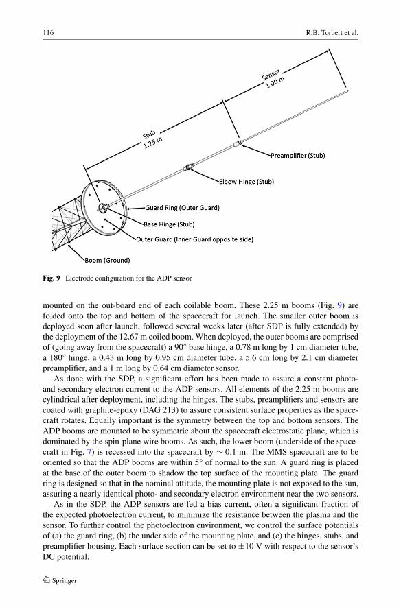
Fig. 9 Electrode configuration for the ADP sensor

mounted on the out-board end of each coilable boom. These 2.25 m booms (Fig. 9) arefolded onto the top and bottom of the spacecraft for launch. The smaller outer boom isdeployed soon after launch, followed several weeks later (after SDP is fully extended) bythe deployment of the 12.67 m coiled boom. When deployed, the outer booms are comprisedof (going away from the spacecraft) a 90° base hinge, a 0.78 m long by 1 cm diameter tube,a 180° hinge, a 0.43 m long by 0.95 cm diameter tube, a 5.6 cm long by 2.1 cm diameterpreamplifier, and a 1 m long by 0.64 cm diameter sensor.

As done with the SDP, a significant effort has been made to assure a constant photo-and secondary electron current to the ADP sensors. All elements of the 2.25 m booms arecylindrical after deployment, including the hinges. The stubs, preamplifiers and sensors arecoated with graphite-epoxy (DAG 213) to assure consistent surface properties as the space-craft rotates. Equally important is the symmetry between the top and bottom sensors. TheADP booms are mounted to be symmetric about the spacecraft electrostatic plane, which isdominated by the spin-plane wire booms. As such, the lower boom (underside of the space-craft in Fig. 7) is recessed into the spacecraft by ∼ 0.1 m. The MMS spacecraft are to beoriented so that the ADP booms are within 5° of normal to the sun. A guard ring is placedat the base of the outer boom to shadow the top surface of the mounting plate. The guardring is designed so that in the nominal attitude, the mounting plate is not exposed to the sun,assuring a nearly identical photo- and secondary electron environment near the two sensors.

As in the SDP, the ADP sensors are fed a bias current, often a significant fraction ofthe expected photoelectron current, to minimize the resistance between the plasma and thesensor. To further control the photoelectron environment, we control the surface potentialsof (a) the guard ring, (b) the under side of the mounting plate, and (c) the hinges, stubs, andpreamplifier housing. Each surface section can be set to ±10 V with respect to the sensor’sDC potential.


The ADP on MMS is expected to measure the DC electric field with an accuracy of∼ 1 mV/m, a resolution of 0.026 mV/m, and a range of ∼ ±1 V/m in most of the plasma en-vironments that MMS will encounter. Constant offsets between the booms will be removedby two methods: namely, minimizing E · B as measured by the double probe over long(> 20 s) periods and comparison with EDI electric field measurements. The spectral powerdensity has a dynamic range from 4 × 10−16 (V/m)2/Hz to 10−3 (V/m)2/Hz at 10 kHz.

3.5 Electron Drift Instrument

EDI determines the electric and magnetic fields quite differently from all the sensors above.It is basically a geometric measurement for the electric field and a timing measurement forthe magnetic field. As seen in Fig. 10, two electron beams are emitted in nearly oppositedirections from two Gun-Detector Units (GDU) on opposite sides of each spacecraft. Eachbeam drifts in the E × B direction and, if properly directed, returns to the spacecraft afternearly one or more gyroperiods. If the drift-step (d = drift velocity, vd , times gyroperiod)is of the order of the baseline separation of the two GDU’s, then the electric field is deter-mined by triangulation as seen in Fig. 11. In this figure, the first GDU (G1) emits a beamin the direction V1 that is detected by the opposite detector, D, and vice versa for G2. The

Fig. 10 Electron beam paths

Fig. 11 Geometry of drift vectorfor EDI


drift step is the displacement of the intersection of the two beams (S) from the position ofthe detector. The actual geometry is slightly more complicated in that the detector for G1

is located at G2 and vice versa. The beams are pseudo-noise encoded so that the emittedelectrons can be unambiguously detected in the presence of ambient electrons, and the timeof flight of the beam can be determined. The difference of the time of flight of the twobeams gives the magnitude of the drift step (which can be used in the “time-of-flight” modewhen the drift step is large compared to the baseline) and the average of the two times givesthe gyroperiod. From the gyroperiod, the magnitude of the magnetic field is determined,and from the directions of the successful beams, the direction of the magnetic field can becomputed. The advantage of EDI over conventional electric and magnetic sensors is thatthe effects of the fields far from the spacecraft dominate the resulting vectors: electrostaticand noise magnetic fluctuations of the spacecraft have little effect when the gyroradius is oforder kilometers, as is the case for MMS. But EDI also has a very slow time cadence fora full vector determination (of order 10 samples per sec) compared to AFG, DFG, SCM,SDP, and ADP. By combining multiple techniques, as described below, improved accuracycan be obtained with high time resolution. The requirements on FIELDS as a whole for anelectric field accuracy of 0.5 mV/m and a magnetic field accuracy of 0.1 nT can thus be met.In order to detect the weak (∼ 100 nA) electron beams emitted by the guns, the detectorof EDI has very large geometric factor (order 0.01 cm2 str) so that very fast sampling ofambient electrons is possible at a fixed energy and for a few directions. Thus, 0.5 or 1 keVelectron fluxes can be determined in the “ambient” mode at 1024 samples per sec and verythin electron layers can be detected.

3.6 Central Electronics Box

The CEB directs all the activities of the FIELDS sensors and formats both housekeeping andscience data for transmission to the CIDP and eventually to the downlink for ground pro-cessing. As diagrammed in Fig. 12, the operating system in CDPU (RTEMS) structures theflight software activities, and allows for command handling (CMD) by non-maskable inter-rupts (NMI) and memory error checking (EDAC). All magnetometer data comes from AFG

Fig. 12 Data procession path within the CEB


Fig. 13 Magnetic sensor system

Fig. 14 Electric sensor system

and DFG as a continuous stream of 128 vectors per second. The CEB performs digital fil-tering on this data down to the commanded rate and also internal coordinate system rotationof the field components for use by FIELDS and other on-board instruments on MMS. Therelevant coordinate systems are seen below (Figs. 13 and 14). The CEB directs the traffic ofEDI and DSP data, and uses some of those data for internal calculations of the Trigger DataNumbers that are used in the ground algorithms to determined selection of BURST data. Italso houses the Low Voltage Power Supply (LVPS) that controls all power distribution inFIELDS as well as the floating power supplies that drive both the SDP and ADP sensors.

Each of the FIELDS sensors can produce data over a large range of sampling rates, asseen in Table 1. In addition, all the DSP input channels (SCM, Vx, Eij , and Eij_AC) areused to produce spectral products over a time series of 1024 samples which are then averagedand sent down as a frequency spectrum (magnitude only). Ancillary data include in-flightcalibration data for SDP, ADP, and SCM, and timing information in the housekeeping data.There are also specialized data products of the DSP that are short samples of all inputs at


Table 1 Possible sample ratesfor sensors within FIELDS Quantity Samples/s

Minimum Maximum

AFG 1, 2, 3 8 128

DFG 1, 2, 3 8 128

DSP inputs

SCM 1, 2, 3 0.5 16384

V1, V2, V3, V4, V5, V6 0.5 16384

E12, E34, E56 0.5 16384

E12AC, E34AC, E56AC 8 262144

V1AC, V2AC 8 262144

High speed burst data

E12_AC, E34_AC, E56_AC 32768 262144

V1_AC, V2_AC 32768 262144

SCM 1, 2, 3 4 16384

EDI modes

E Field mode: beam pairs Variable 125

Ambient mode: flux samples 4 1024

very high rates, but only small duty cycles. These include the High Speed Burst channels(HSB-E and HSB-B) as well as the output of a Solitary Wave Detector algorithm.

Depending on the science questions to be addressed, a very large number of possibletelemetry modes can be constructed by ground command. These are limited only by thetotal bit rate allocation for FIELDS seen in Table 3. As described in a companion paper onBURST mode (Fuselier et al. 2014, this issue), the CEB executes two basic modes, Slowand Fast Survey, and produces continuous data products that are always telemetered to theground. In addition, very high data rate “BURST” products are produced only in Fast Surveymode and sent to the CIDP for storage. Only interesting intervals of this data are selected forground transmission because there is not enough overall telemetry to accommodate BURSTmode data over the full orbit. At launch, there are two modes for the BURST data: one fordayside reconnection studies in Phase 1 and one from the magnetotail studies in Phase 2.These default sampling modes, which can be changed or replaced in flight, are listed inTable 2 (nominal duty cycles for HSB are indicated as percentages).

The overall resource utilization of FIELDS is given below. The masses do not includethose for spacecraft harness or magnetometer booms.

4 Timing

A central design goal of the FIELDS suite requires that its sensors are sampled on the samesynchronous time base defined by the FIELDS independent clock. The FIELDS clock runsasynchronously to those in the CIDP and the spacecraft, thus requiring FIELDS time to becontinually interpreted and cast in absolute terms. An absolute time reference is provided bythe spacecraft GPS unit (the Navigator) and is distributed throughout the spacecraft. It con-sists of a one pulse per second (PPS) timing signal and the associated TAI time at the pulse.Correlation data contained within instrument housekeeping and instrument characteristics


Table 2 Nominal modes of FIELDS CEB

Quantity Type Components Samples/s

Slow survey Fast survey Burst-phase 1 Burst-phase 2

EDI Coded Beam pair ∼16 ∼16 ∼125 ∼125

AFG Time series 3 8 16 128 128

DFG Time series 3 8 16 128 128

DC-E Time series 3 8 32 1024 8192

AC-E Time series 3 8192 8192

DC-V Time series 1 to 3 8 32 1024 8192

SCM Time series 3 8 32 1024 8192

LFE Spectra 1 or 3 0.0625 0.5

MFE Spectra 1 or 3 0.0625 0.5

LFB Spectra 1 or 3 0.0625 0.5

HSB-E Time series 3 65536@40 % 65536@10 %

HSB-B Time series 3 16384@40 % 16484@10 %

Table 3 Resources for theFIELDS suite Component Power (W) Mass (kg)

Slow survey Fast survey

CEB 8.443 8.610 5.37

SDP 1.829 1.829 17.20

ADP 0.857 0.857 15.48

SCM 0.181 0.181 0.91

EDI 3.430 4.850 11.90

AFG in CEB 0.74

DFG in CEB 0.74

Totals 14.740 16.327 52.34

Data rates Slow survey Fast survey Burst

kbits/s 2.36 7.93 843.61

are used to assimilate FIELDS time with the TAI information. The correction of FIELDStime into absolute terms is performed as part of ground processing. The FIELDS DSP andEDI components can be timed between themselves to better than 20 µs and to within 50 µsto the flux-gate magnetometers, which have a larger sample times of ∼ 8 ms. This greatlysimplifies inter-sensor calculations of Poynting vectors, current sheets relative to electronfluxes seen by EDI, the algorithms that combine EDI, ADP, and SDP into one electric fieldrecord, and the algorithms that combine AFG, DFG, SCM, and EDI into one magnetic fieldrecord, as described below.

To assure this intra-sensor timing knowledge, an extensive suite of calibrations was con-ducted as part of the FIELDS Interference and Timing (FIT) campaign. This campaign con-sisted of two main parts: 1) an interference assessment to verify FIELDS self-compatibilityand 2) a timing investigation to verify time tag accuracy, which is described here, andFIELDS-level frequency response of sensors. The timing investigation was divided intothree specialized tests to address the specific workings of the electric field instruments (ADP


Fig. 15 Multiple PPSmeasurements taken by DSPSN12 with the idealized PPSpulse location (red)

Table 4 Time corrections applied to DSP data displayed in Fig. 14

PPS & Signal propagation delay description Corrective value

PPS pulse transmission delay 23.7 µs

DSP expected analog delay −60.6 µs

DSP ADC acquisition, sample and hold delay −3.3 µs

DSP Mux delay: 3.8 µs ∗ (Channel-1). Zero for first sampled channel +0 µs

DSP digital delay (16 kS/s sampling) −183 µs

Total scalar timing adjustments −223.2 µs

Frequency offset between FIELDS clock and PPS clock. Clock rate difference driftsthroughtout testing due to temperature dependence. This effect is corrected for usinginformation from FIELDS housekeeping packets

0 to 5 µs (variable)

and SDP), magnetometers (AFG, DFG, and SCM) and EDI. In each of these tests, sensorresponses to calibrated, PPS-synchronous stimuli were recorded. The results were analyzedfor time tag accuracy and precision and compared to the expected frequency response of theinstrument.

4.1 DSP Timing

The ADP, SDP and SCM data time tags, which are provided by the DSP, were verified by theDSP direct-measurement of the PPS timing events. Known timing delays and advances fromthe PPS broadcast, data sampling, and coarse-fine time clock differences displace the timetag from the nominal value. The difference between the expected and measured PPS eventtime tags is a measure of the timing tagging accuracy. The jitter in the measured PPS eventtime tags is an estimate of the time tagging precision. Figure 15 shows 250 PPS measure-ments overlaid with the whole seconds removed and adjustments made for the known delayslisted in Table 4. The 90-µs wide PPS pulse was not well-resolved by the 16 kS/s (60 µs)sampling of these tests. However, the center of the measurement still corresponds with thecenter of the PPS pulse. Since the rise of the PPS is what marks the start of a whole second,the corresponding location of the measured PPS was calculated by subtracting half the PPSpulse width (45 µs) from the time associated with the weighted center. This calculation wasperformed on each measured PPS event; the average and standard deviation of the resultantvalues are used to describe the distribution. DSP flight model #12 (FM12) measurementsare shown here to have an unaccounted delay of −4.7 ± 2.0 µs, which is within the rangethat may be expected with jitters of up to 5 µs in the relative clocks.


Since the DSP time tags only the first sample of each data packet, the times of subsequentsamples are assigned during ground processing, based on the channel sample rate and clockrate differences between the FIELDS and spacecraft (GPS) clocks. (Note that the clock ratedifference is calculable, using the time tags from FIELDS housekeeping packets.) Stimulusapplied at the top of a second is often placed in a packet with a time tag near the end of theprevious second. This maximizes the time tagging error, so the values produced from thismethod are taken as the worst case.

4.2 AFG and DFG Timing

The AFG and DFG time tags are verified with known PPS-synchronous current stimulus,driven through test coils in a magnetically shielded environment and simultaneously mea-sured by the sensors and a DSP channel. Differences in the sensor and DSP response to thestimulus, after adjusting for known timing advances and delays, are used to characterize theAFG and DFG time tags. The current generator test equipment provides arbitrary currentand voltage stimuli with known timing relation to the PPS tone. The frequency responses ofthe magnetometers have been characterized with this current generator through two differentmethods.

Noise Cross Spectra: Pink and white noise signals were applied to the magnetic fieldsensors. The stimulus current was simultaneously recorded by a DSP channel, thus provid-ing a time-accurate record of the stimulus applied to the sensors. Cross spectra calculationsbetween the sensor-measured magnetic field and the independent DSP-measured referenceprovided the frequency response of the AFG, DFG and SCM sensors.

Sine Fit: A sine wave with known frequency and amplitude was applied to the test coil viathe current generator. The sine signal was synchronized to the PPS tone with a well-definedphase relation. The sensor delay was determined as the difference between the phase of themeasurement relative to the PPS via a numerical fit and the known phase relation of thestimulus.

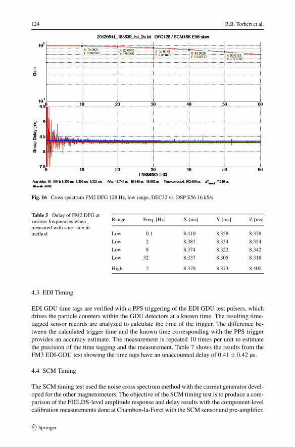
Both methods were performed with the DFG and AFG sensors in the different permu-tations of range (high or low) and sampling rate (8, 16, 32, 64 and 128 Hz). DFG mea-surements were also performed in the different DEC (digital filter length, see Russell et al.2014, this issue) modes (32 or 64), while AFG measurements were performed with bothADCs (A or B). The two measurement methods produce results within the range of ex-pected values for all cases. Figure 16 shows the FM2 DFG noise cross spectrum results with128 Hz sampling, low range and DEC32 modes. The delays for the x, y and z axes were8.353, 8.303 and 8.321 ms, respectively. The expected value given known system delays is8.308 ms ±30 µs, which is in agreement with the noise cross spectrum measurement.

Table 5 shows the FM2 DFG sine fit results for time delays for the difference ranges at se-lected frequencies. The delays measured with the sine fit method are about 20 − 30 µs largerthan those measured with the noise—cross spectra method. The source of the discrepancyis not known, however both methods are within the range of the expected value.

Figure 17 shows the FM2 AFG noise cross spectrum results with 128 Hz sampling, lowrange and ADC-A. The delay for the x, y and z axes between 2–10 Hz was measured to be11.425, 10.808 and 10.717 ms, respectively.

Table 6 shows the FM2 AFG sine fit results for the difference ranges at selected frequen-cies. Similar to the DFG results, the delays measured with the sine fit method are about20–30 µs larger than those measured with the noise—cross spectra method. The source ofthe discrepancy is not known, however both methods verify the expected value well withinthe requirement measurement offsets.


Fig. 16 Cross spectrum FM2 DFG 128 Hz, low range, DEC32 vs. DSP E56 16 kS/s

Table 5 Delay of FM2 DFG atvarious frequencies whenmeasured with sine–sine fitmethod

Range Freq. [Hz] X [ms] Y [ms] Z [ms]

Low 0.1 8.410 8.358 8.378

Low 2 8.387 8.334 8.354

Low 8 8.374 8.322 8.342

Low 32 8.337 8.305 8.318

High 2 8.370 8.373 8.400

4.3 EDI Timing

EDI GDU time tags are verified with a PPS triggering of the EDI GDU test pulsers, whichdrives the particle counters within the GDU detectors at a known time. The resulting time-tagged sensor records are analyzed to calculate the time of the trigger. The difference be-tween the calculated trigger time and the known time corresponding with the PPS triggerprovides an accuracy estimate. The measurement is repeated 10 times per unit to estimatethe precision of the time tagging and the measurement. Table 7 shows the results from theFM3 EDI-GDU test showing the time tags have an unaccounted delay of 0.41 ± 0.42 µs.

4.4 SCM Timing

The SCM timing test used the noise cross spectrum method with the current generator devel-oped for the other magnetometers. The objective of the SCM timing test is to produce a com-parison of the FIELDS-level amplitude response and delay results with the component-levelcalibration measurements done at Chambon-la-Foret with the SCM sensor and pre-amplifier.


Fig. 17 Cross spectrum FM2 AFG 128 Hz, low range, ADC A vs. E56 16 kS/s; (blue) X, (green) Y, (red) Z

Table 6 Delay of FM2 AFG atvarious frequencies whenmeasured with sine fit method

Range Freq. [Hz] X [ms] Y [ms] Z [ms]

Low 0.1 11.470 10.860 10.785Low 2 11.449 10.817 10.728Low 8 11.397 10.777 10.691Low 32 10.916 10.446 10.358

High 2 11.452 10.819 10.732

Table 7 FIT test results for FM3 EDI-GDU

No. EDI packetcoarse time

EDI packetfine time(raw)

Transitionalcounts index

Transitionalcounts value

Fullcountsvalue

Predicted timeof 1PPS

Nominal1PPS

Deviationfrom fullsecond [µs]

1 404 343922 673 172 1024 405.00000015 405 0.152 438 343906 673 156 1024 438.99999941 439 −0.593 474 343893 673 142 1024 474.99999976 475 −0.244 504 343883 673 132 1024 504.99999929 505 −0.715 529 343877 673 125 1023 529.99999985 530 −0.156 554 343871 673 119 1023 554.99999957 555 −0.437 579 343867 673 114 1023 580.00000034 580 0.348 604 343863 673 111 1024 604.99999932 605 −0.689 624 343861 673 109 1024 624.99999923 625 −0.77

10 644 343859 673 107 1023 644.99999902 645 −0.98

Result 0.41 ± 0.42


Fig. 18 Cross spectrum SCM 16 kS/s, DSP A vs. E56 16 kS/s; (blue) X, (green) Y, (red) Z

The difference between these two tests is the presence of the DSP, which contributes addi-tional attenuation and delays due to analog and digital filters. The SCM noise cross-spectrummeasurements were performed over different sampling rates (1, 8, and 16 kSamples/s) andfor both of the redundant DSP boards. Figure 18 shows the FM3 results with 16 kS/s sam-pling and DSP-A plotted with the calibration results from Chambon-la-Foret. The zoom plotshows a 210 µs offset in the measured group delays. This additional delay of the digitized


Table 8 FIELDS routine data products

Sensor (s) Description

FIELDS Quicklook products

AFG 3-component B-field from Analog Flux Gate (AFG), to 16 vectors/s

DFG 3-component B-field from Digital Flux Gate (DFG), to 16 vectors/s

SDP-ADP 3-component E-field from Spin-plane Double Probe (SDP) and Axial Double Probe(ADP), to 32 samples/s

SDP-ADP 3-component Low Frequency (LF) electric spectra, 1–8000 Hz

SDP-ADP 3 sampled Medium Frequency (MF) electric spectra, 25–100 kHz

SCM 3-component LF magnetic spectra, 2–6000 Hz

EDI Ambient electrons at two directions

FIELDS Level 2 products

AFG 3-component B-field from Analog Flux Gate (AFG), to 128 vectors/s

DFG 3-component B-field from Digital Flux Gate (DFG), to 128 vectors/s

SDP-ADP 3-component E-field from Spin-plane Double Probe (SDP) and Axial Double Probe(ADP), to 8192 samples/s

SDP-ADP 3-component AC E-field from Spin-plane Double Probe (SDP) and Axial DoubleProbe (ADP), to 8192 samples/s

SDP-ADP 3-component high speed burst E-field from Spin-plane Double Probe (SDP) andAxial Double Probe (ADP), to 65536 samples/s

SDP-ADP 1 spacecraft potential sample from combination of ADP and SDP

SDP-ADP 3 sphere voltages from ADP and SDP

SDP-ADP 3-component Low Frequency (LF) electric spectra, 1–8000 Hz

SDP-ADP 3 sampled Medium Frequency (MF) electric spectra, 25–100 kHz

SCM 3-component AC B-field waveform from Search Coil Magnetometer (SCM)

SCM 3-component high speed AC B-field waveform, to 16384 samples/s

SCM 3-component LF magnetic spectra, 2–6000 Hz

EDI Electric fields and drift velocity from Electron Drift Instrument (EDI)

EDI Ambient electrons at two directions

FIELDS Level 2-plus products

AFG-DFG-SCM 3-component combined B-field from all Mag sensors, to 1024 or greater vectors/s

SDP-ADP-EDI 3-component E-field from Spin-plane Double Probe (SDP) and Axial Double Probe(ADP) and Electron Drift Instrument (EDI), to 8192 samples/s

SCM data reflects the delay of the DSP channels, as referenced above in the DSP timingsection.

5 Data Processing and Products

From data obtained in various modes, as seen in Table 2, programmed from possible datachannels as in Table 1, ground processing produces a set of standard FIELDS data productsthat reside in the Science Data Center (SDC) and at the FIELDS Instrument Team Facility(ITF) at UNH.

Level 1 products for FIELDS are produced at the SDC from L0 data with software pro-vided by the FIELDS team. For most of FIELDS data, Level 1 processing consists mostly ofdecompression of data and accurate time tagging for these data using the timing information


Table 9 In-flight calibration methods

Calibrated item Comparator Method Frequency

AFG/DFG orthogonality None Spin plane quadrature,Spin-tone removal

Every orbit

AFG/DFG gains and offsets ObservatoryAFG/DFG

Inter-observatory comparison Monthly, or as needed

AFG/DFG gains Spin-planereference phase

Perigee pass analysis Initial, quarterly or higherphase 1, 2

FG offsets None Variance analysis, Solar Wind Yearly, as availableFG spin-axis offsets EDI Direction, TOF comparison WeeklySCM gains AFG, DFG Overlapping frequency band MonthlySCM gains, phase, offsets None Waveform analysis of cal

signalsDaily

SDP, ADP gains AFG, DFG −Vsc × B perigeecomparison

Initial, monthly phase 1, 2

SDP, ADP gains FPI, HPCA Solar Wind −V × Bcomparison

As available

SDP, ADP gains, offsets EDI Direct Eperp comparison Continual, distinguishingdifferent plasma regimes

SDP, ADP offsets DFG, AFG E · B = 0 check Quiet regionsSDP, ADP offsets HPCA −VO+ × B comparison Lobe outflow regionsEDI MCP gains None Ambient response: MCP,

pre-ampMonthly

from sensors and the FIT tests described above. In some cases, there is a Level 1b data setwhere initial and tentative calibrations are applied for use in early processing.

The QuickLook and Level 2 products are produced initially using the best ground cali-brations available for each sensor and then are combined in the manner that has been usedin many previous missions such as Cluster, Polar, and THEMIS. QuickLook is availablewithin 24 hours after the receipt of data; and Level 2, within 30 days. The FIELDS coordi-nate systems for this processing have been carefully co-aligned on the ground and are usedfor production of the first stage of this processing, and then rotated into the GSE coordinatesystem for science use.

For Level 2, the ground calibrations are augmented with an extensive set of on-orbit cal-ibrations as listed in Table 9. During the mission, weekly conferences of both the magneticfield team and the electric field team on MMS will use these techniques to improve theoverall accuracy of L2 data.

For MMS, the integrated FIELDS suite allows the combination of these products usingnew algorithms such as described below to achieve the accuracy needed for MMS. Theseproducts are listed as Level 2-Plus above and the production algorithms are described below.

FIELDS also contributes to the calculation of MMS Level 3 data products obtained froma combination of the data from different instruments. Seven parameters use FIELDS data:electron number density (from selected periods where the upper hybrid resonance frequencycan be identified); Alfvén speed; E × B velocity; E + Ve × B; plasma beta; and energeticion and electron anisotropy.

5.1 Combination Algorithms

To provide the environment for highly accurate magnetic field data from the combination ofEDI, AFG, DFG, and SCM, the observatories must meet strict magnetic cleanliness require-


ments, as mentioned above. These requirements and how they were achieved and confirmedare described in Russell et al. (2014, this issue). The care taken to ensure that EDI, AFG,DFG and SCM are intercalibrated and accurately temporally referenced is described above.A complementary science objective is that the measurements across spacecraft be intercali-brated. For the fluxgate magnetometers, intercalibration is especially important for they areused to determine the currents that are flowing on the plasma boundaries. The intercalibra-tion techniques for the magnetometers by themselves are described further in Russell et al.(2014, this issue). The procedures for combining data from the various FIELDS sensors areoutlined here.

5.1.1 Magnetometer Spin-Axis Offset Determination

The magnetometer and EDI teams will use the EDI beam data, consisting of both electrongyro-periods and directions of the beam perpendicular to B , in an intensive collaborativeeffort to determine the spin axis offsets of the flux-gate (FG) magnetometers AFG and DFG(also used by SCM). In most previous satellite measurement sets, the generally used methodsfor in-flight determination of FG magnetometer spin axis offsets are based on the analysisof Alfvénic fluctuations in the solar wind. As MMS excursions into the solar wind will onlybe an exception in early mission phases, the spin-axis offsets will have to be determined bycomparison with EDI data. Electron times-of-flight (TOFs) are inversely proportional to thestrength of the ambient magnetic field. Furthermore, EDI beam firing directions (BDs) haveto be perpendicular to that field for the beams to return to the spacecraft. Hence, comparisonof both quantities, TOFs (T ) and BDs ( �D) to FG magnetic field measurements ( �B) can yieldspin axis offsets, if the FG data are sufficiently well calibrated for EDI to work at all. Here,we briefly describe the TOF and BD methods; more details can be found in Plaschke et al.(2014).

In the TOF method, the FG spin axis offsets are determined based on comparison be-tween the FG magnetic field and the magnetic field magnitude deduced from EDI TOFs(Georgescu et al. 2006; Leinweber et al. 2012; Nakamura et al. 2014). As discussed inNakamura et al. (2014), EDI TOFs may themselves be subject to offsets, which depend onindividual sensor (GDU) and the mode of operation. Systematic TOF offsets can be obtainedby comparison with �B vectors that lie close to the spin plane, so that | �B| is not much affectedby spin axis offset uncertainties:

δT = T − k

| �B|OT = median(δT )

Here δT is the TOF offset determined from a pair of T and �B measurements, k is a conver-sion factor between TOFs and magnetic field strengths, and OT is the GDU/mode specificTOF offset, which the respective EDI measurements are to be adjusted with: Tc = T − OT .As described in Plaschke et al. (2014), the median offsets OT are determined from a largedata set of measurements. Spin axis offset estimates are then obtained from adjusted TOFsby:

OSA = BSA − sign(BSA)

√k2

T 2c

− B2SP

Here, the indices SA and SP denote spin axis and spin plane components, respectively.


In the BD method, the FG spin axis offsets are determined based on the perpendicularityof BD and magnetic field. Ideally, the angle α between �D and �B is 90°. The BD methodis not affected by TOF offsets, but requires accurate transformations of �D and �B into acommon, spacecraft-fixed, and spin aligned coordinate system. The GDU-specific transfor-mations can be adjusted by minimization of (α − 90°)2, where the angles α are computedfrom near-spin-plane BDs �D (least affected by FG spin axis offsets). FG spin axis offsetestimates are then obtained by:

OSA = �B · �DDSA

The TOF and BD methods for spin axis offset determination are complementary withrespect to the directions of �D and �B . The TOFs are compared to FG measured | �B| values,which are most affected by offsets if �B points in spin axis direction. Instead, BDs are mostsensitive to changes in offsets if directed toward the spin axis. These conditions are mutuallyexclusive as �D⊥ �B . Consequently, by combining these two methods taking into account thedifferent sensitivity dependence to the field conditions, a comprehensive scheme of offsetdetermination will be performed.

5.1.2 AFG-DFG-SCM Combination

Electron diffusion regions and thin current sheets pass over the MMS spacecraft in timeintervals of 0.5 to 2 seconds because a typical region size of 5 to 20 km moves with aboundary speed of 10 to 100 km/sec. See, for example, Fig. 2. The frequency range of 0.5to 20 Hz transitions from a low-frequency boundary where the SCM has little signal to ahigh-frequency one where the FG loses its ability to accurately track fields that vary thisfast. Thus, on MMS, it is critical to have algorithms to combine these two measurementsin this overlapping frequency band into one accurate data series. We use two methods: onetime-domain and one frequency domain.

Both methods rely on preprocessing of the data by standard methods, which includestime tagging, offset and maximum gain correction, orthogonalization and transformation toa common coordinate system for both FG and SCM signals. For this purpose data fromground and inflight calibration are used, including also data from EDI.

The frequency domain algorithm applies a Tukey window to the data, which has unitygain at the central half of the data. Each data set is then Fourier transformed and correctedwith the amplitude and phase responses found during ground individual and cross calibra-tion. At this point, the spectra are compared for consistency over the overlap frequency rangefrom 0.2 Hz to 64 Hz to assure correct processing.

The two complex frequency spectra are now merged as follows. Below a lower transitionfrequency (∼ 0.5 Hz, well above the spin frequency), we use the FG data exclusively. Above16 Hz, we use the SCM data exclusively. Between these two frequencies, we use a weightedaverage of the two, with the weight determined by the amount that the individual powerspectra exceeds the determined noise power threshold. These thresholds are determined bya statistical histogram of power at various frequencies, with data taken over selected quietintervals. This new combined spectrum is then reverse Fourier transformed, window cor-rected, and then rotated into the spacecraft coordinate system. Now, only the central halfof this time interval is used for the final data. At the beginning and end segments of anyanalysis interval, the first quarter and last quarter of those respective segments are used aswell.


Fig. 19 Results of FG/SCMcombination algorithm

The time domain algorithm is based on adapting compensation filters in a way that thetotal response of each instrument has a selected low-pass (FG) or high-pass (SCM) charac-teristic. Those filters are chosen such that their summed response is close to unity gain andlinear phase within the whole band of interest of the combined data product. The crossoverfrequency (cutoff of both filters) is a parameter that can be chosen dependent on noise powercomparison of both instruments.

The combined data product can then be calculated by converting both signals to a com-mon sampling base, applying the relevant filters and merging the signals. To minimize theinfluence of filtering on short bursts of higher frequency, the previous low frequency data isused to preload the filters.

In principle both are approaching the same problem with different focus. The frequencydomain algorithm is concentrated on getting the minimum noise power within the combinedsignal, whereas the time domain algorithm is focused on creating a signal without side-effects (pre- and post-echo) caused by signal processing, but at the price of higher noise.

The frequency domain algorithm has already been applied to both Cluster test data andcalibration data from the MMS FIT tests, as seen in Fig. 19, where DFG and SCM data havebeen combined.

Although the test configuration did not allow proper coordinate system rotations, all thetiming delays described above and the measured transfer functions were used to implementthe combination procedure to test how well MMS resolves sharp transitions of the magneticfield. The close correspondence of the driving field current (green trace) and the merged datashow that sharp structures with time durations well below 5 ms can be reconstructed.

Further investigations of data gained during the FIT tests are still ongoing to get bettermodels for the frequency properties of the instruments.

5.1.3 SDP-ADP-EDI

Using all three axes of ADP/SDP, a full vector electric field can be constructed at the fullsample rate of the DSP (up to 16384 samples/s, or higher if need be). However, the Double-probe method is susceptible to well-known offsets due to electric fields induced by pho-toemission charges and the resulting electron cloud, and to wake effects of the satellite as


Fig. 20 Analysis of E × B driftin the Bperp plane

it moves through the ambient plasma. Due to the fact that the electron beam spends mostof its time well away from the spacecraft, EDI is not affected by these offsets, but is ableto produce a field value only perpendicular to the magnetic field at about 10 samples/s. Toachieve the 0.3 mV/m accuracy, which is the MMS goal, we must combine these measure-ments to produce an accurate high-rate field measurement and to estimate the error in thatmeasurement. A new algorithm, called BESTARG2, has been developed to do this.

For the first step, the field values from ADP/SDP and EDI are compared to remove thewell-known sun-aligned (or GSE-X) component offset in the DP measurement that resultsfrom the local photoelectron cloud. A smoothing algorithm produces a slowly varying valuefor this offset and then removes it from the DP component. Then the DP 3D field valueclosest to a single EDI beam is projected into the plane perpendicular to B and used toproduce a drift step “target” such as EDI measures (drift step d = drift velocity, vd , timesgyroperiod, see Fig. 11). As the spacecraft turns, the GDU’s move on the boundary of theshaded ellipse in the Bperp plane. Level 2 data from EDI uses multiple beams from bothGDU’s to determine the drift step, as seen in Fig. 11 above, but by using every single beam,BESTARG2 is able to compare fields on a much faster time cadence. The true target mustlie somewhere on the beam line, and if there were simultaneously two EDI beams, theywould be at the intersection of the two beams. The composite field value is determined bydisplacing the DP drift step by the minimum amount to move it onto the single beam line,and the error is estimated by the length of that displacement (see Fig. 20).

The BESTARG2 analysis was performed on several intervals of Cluster data using EFW(the equivalent to SDP) and EDI when the magnetic field was mostly perpendicular to thespin plane so that both techniques were measuring in the Bperp plane. The results are givenin Fig. 21. Here the black trace in the upper panel is the initially corrected L2 data from thedouble probes. The above algorithm then produces the magenta trace in the middle panel.The estimated resulting error is plotted in the lower panel, showing that errors of less than0.5 mV/m are possible.


Fig. 21 Results of combining EDI with EFW on Cluster using BESTARG2

During the MMS mission, a study of the resulting errors, taking into account bias levelson the ADP/SDP and plasma environmental conditions may lead to a better understandingof the origin of the error and its reduction by different biasing schemes on the DP electrodesand/or better beam detection schemes on EDI.

6 Conclusion

With its highly integrated and inter-calibrated suite of sensors, the FIELDS instrumentationis well constructed to fulfill its requirements. The precise measurement of the fully 3D elec-tric and magnetic fields will allow MMS to map magnetic topology and resolve structuresof the electron and ion diffusion regions; determine the motion and orientation of bound-aries such as the magnetopause and the magnetotail current sheets; establish mass flow ratesacross magnetopause during reconnection; and determine the breaking of the frozen-in flowvelocity and the divergence of Poynting flux across the reconnection boundary. Combining


all the capabilities of the FIELDS suite with those of the particle instrumentation on fourversatile satellites, MMS provides a mission to advance significantly our understanding ofmagnetic reconnection.

Acknowledgements Development of the FIELDS instrumentation suite has been the joint effort of manygroups within the authors’ institutions over the last 15 years. We acknowledge here generous support by theSpace Science Center and the EOS Institute at UNH and the many staff members who gave a great partof their careers in the development of MMS. We wish to thank the generous assistance of technical andmanagement staff at NASA GSFC and at SwRI, in particular W.C. Gibson and R.K. Black for managing theentire SMART instrument suite. FIELDS was developed under NASA MMS contract NNG04EB99C via theSwRI subcontract to UNH.

Open Access This article is distributed under the terms of the Creative Commons Attribution Licensewhich permits any use, distribution, and reproduction in any medium, provided the original author(s) and thesource are credited.

References

M. Andre, A. Vaivads, S.C. Buchert, A.N. Fazakerley, A. Lahiff, Thin electron-scale layers at the magne-topause. Geophys. Res. Lett. 31, L03803 (2004). doi:10.1029/2003GL018137

T.G. Cowling, Solar electrodynamics, in The Sun, ed. by G.P. Kuiper (University of Chicago Press, Chicago,1953), pp. 532–591

J.F. Drake, Particle heating and acceleration in magnetic reconnection, in Magnetic Reconnection: An Inter-disciplinary Workshop, Yosemite, CA (2010)

J.W. Dungey, Conditions for the occurrence of electrical discharges in astrophysical systems. Philos. Mag.44, 725–739 (1953)

J.W. Dungey, Interplanetary magnetic field and the auroral zones. Phys. Rev. Lett. 6, 47–48 (1961)J. Egedal, W. Daughton, A. Le, Large-scale electron acceleration by parallel electric fields during magnetic

reconnection. Nat. Phys. (2012). doi:10.1038/NPHYS2249U. Fahleson, Theory of electric field measurements conducted in the magnetosphere with electric probes.

Space Sci. Rev. 7, 238–262 (1967)S.A. Fuselier, W.S. Lewis, C. Schiff, R. Ergun, J.L. Burch, S.M. Petrinec, K.J. Trattner, Magneto-

spheric multiscale science mission profile and operations. Space Sci. Rev. (2014, this issue). doi:10.1007/s11214-014-0087-x

E. Georgescu, K.-H. Fornacon, U. Auster, A. Balogh, C. Carr, M. Chutter, M. Dunlop, M. Förster, K.-H.Glassmeier, J. Gloag, G. Paschmann, J. Quinn, R. Torbert, Use of EDI time-of-flight data for FGMcalibration check on Cluster, in Proceedings of the Cluster and Double Star Symposium 5th Anniversaryof Cluster in Space (ESTEC, Noordwijk, 2005)

E. Georgescu, H. Vaith, K.-H. Fornacon, U. Auster, A. Balogh, C. Carr, M. Chutter, M. Dunlop, M. Foerster,K.-H. Glassmeier, J. Gloag, G. Paschmann, J. Quinn, R. Torbert, Use of EDI time-of-flight data forFGM calibration check on Cluster, in Cluster and Double Star Symposium. ESA Special Publ., vol. 598(2006)

R.G. Giovanelli, A theory of chromospheric flares. Nature 158, 81–82 (1946)M. Hesse, N. Aunai, J. Birn, P. Cassak, R.E. Denton, J.F. Drake, T. Gombosi, M. Hoshino, W. Matthaeus, D.

Sibeck, S. Zenitani, Theory and modeling for the magnetospheric multiscale mission. Space Sci. Rev.(2014, this issue). doi:10.1007/s11214-014-0078-y

F. Hoyle, Magnetic storms and aurorae, in Some Recent Researches in Solar Physics (Cambridge UniversityPress, Cambridge, 1949), pp. 92, 102–104

H.K. Leinweber, C.T. Russell, K. Torkar, In-flight calibration of the spin axis offset of a fluxgate mag-netometer with an electron drift instrument. Meas. Sci. Technol. 23, 105003 (2012). doi:10.1088/0957-0233/23/10/105003

F.S. Mozer, S.D. Bale, T.D. Phan, Evidence of diffusion regions at a subsolar magnetopause crossing. Phys.Rev. Lett. 89, 015002 (2002)

R. Nakamura, F. Plaschke, R. Teubenbacher, L. Giner, W. Baumjohann, W. Magnes, M. Steller, R.B. Torbert,H. Vaith, M. Chutter, K.-H. Fornacon, K.-H. Glassmeier, C. Carr, Interinstrument calibration usingmagnetic field data from the flux-gate magnetometer (FGM) and electron drift instrument (EDI) onboardCluster. Geosci. Instrum. Method. Data Syst. 3, 1–11 (2014). doi:10.5194/gi-3-1-2014

http://dx.doi.org/10.1029/2003GL018137

http://dx.doi.org/10.1038/NPHYS2249

http://dx.doi.org/10.1007/s11214-014-0087-x

http://dx.doi.org/10.1007/s11214-014-0087-x

http://dx.doi.org/10.1007/s11214-014-0078-y

http://dx.doi.org/10.1088/0957-0233/23/10/105003

http://dx.doi.org/10.1088/0957-0233/23/10/105003

http://dx.doi.org/10.5194/gi-3-1-2014


E.N. Parker, Sweet’s mechanism for merging magnetic fields in conducting fluids. J. Geophys. Res. 62, 509–520 (1957)

E.N. Parker, Astrophys. J. Suppl. 77 (8), 177 (1963)H.E. Petschek, Magnetic field annihilation, in AAS–NASA Symposium on the Physics of Solar Flares, NASA

SP-50, Washington, DC ed. by W.N. Hess, (1964), pp. 425–439F. Plaschke, R. Nakamura, H.K. Leinweber, M. Chutter, H. Vaith, W. Baumjohann, M. Steller, W. Magnes,

Flux-gate magnetometer spin axis offset calibration using the election drift instrument. Meas. Sci. Tech-nol. (2014, submitted)

P.L. Pritchett, F.S. Mozer, Asymmetric magnetic reconnection in the presence of a guide field. J. Geophys.Res. 114, JA014343 (2009)

C.T. Russell, B. Anderson, W. Baumjohann, K. Bromund, D. Dearborn, G. Le, H. Leinweber, D. Leneman,W. Magnus, J.D. Means, M. Moldwin, R. Nakamura, D. Pierce, K. Rowe, J.A. Slavin, R.J. Strangeway,R. Torbert, C. Hagen, I. Jernej, A. Valavanoglou, I. Richter, The magnetospheric multiscale magnetome-ters. Space Sci. Rev. (2014, this issue). doi:10.1007/s11214-014-0057-3

B.U.O. Sonnerup, Reconnection of magnetic fields, in Solar Terrestrial Physics: Present and Future. NASARef. Pub., vol. 1120 (1984). Chap. 1

K. Torkar, R. Nakamura, M. Tajmar, C. Scharlemann, H. Jeszenszky, G. Laky, G. Fremuth, C.P. Escoubet,K. Svenes, Active spacecraft potential control investigation. Space Sci. Rev. (2014, this issue). doi:10.1007/s11214-014-0049-3

http://dx.doi.org/10.1007/s11214-014-0057-3

http://dx.doi.org/10.1007/s11214-014-0049-3

http://dx.doi.org/10.1007/s11214-014-0049-3

the fields instrument suite on mms: scientific …...the fields instrument suite on mms 107 fig. 1...

Documents