The Farm Size-Productivity Relationship in Tanzania: Preliminary Findings

Ayala WinemanThomas S. Jayne

Presented at the Farm Size/Farm Productivity Conference, organized by Economic Research Service, USDA,

Washington, DC, February 1-2, 2017

1

Hypotheses1. IR is a function of market

failures. It will disappear when we account for local levels of land or labor market activity.

2. IR is a function of plot-level characteristics.

It will disappear when we control for time-invariant plot fixed effects.

3. IR is a function of crop mix on small farms/ plots.

It will disappear when we account for crop mix in adequate detail.

2

3

Data

LSMS (NPS) Tanzania 2008/09, 2010/11, 2012/13

Info on area and net value of crop production

Complete info for all RHS variables

Plots tracked from year 2009, present in all 3 survey waves with complete info in all waves

2008/09 4,734 4,401 2,3702010/11 5,412 4,905 2,3702012/13 6,635 6,187 2,370Total 16,781 15,493 7,110Sample restrictions ≤ 50 acres = 15,455 ≤ 50 acres = 7,083

Number of plot-level observations

05

101520253035

< 0.5 0.5-1 1-2 2-3 3-4 4-5 5-7 7-10 10-20 20-40 >=40

% p

lots

Plot size (acres)

Distribution of plot sizes in Tanzania

95th percentile:7.20 acres (2.91 ha)

Relationship between plot area and crop revenue

For visual clarity, sample excludes plots greater than 10 acres.

Net value crop production/ acreCoef P-value

< 0.5 acres -5.31*** 0.000.5-1 -0.88*** 0.001-1.5 0.15 0.421.5-2 -0.50*** 0.0092-3 -0.13* 0.093-4 -0.09 0.314-5 -0.17* 0.085-7 -0.06 0.287-10 -0.07* 0.0610-20 -0.02** 0.0220-40 0.0004 0.96≥ 40 acres -0.002** 0.03Constant 4.83*** 0.00Observations 16,781R-squared 0.08*** p<0.01, ** p<0.05, * p<0.1

Linear piecewise (spline) regression

These coefficients represent the slope at this section of the plot-size spectrum.

Non-parametric polynomial regression

Relationship between plot area and crop revenue– Regression analysis (pooled OLS) –

(1) (2) (3) (4) (5)Dependent variable: Net value crop production/ acre

(100,000s TSh)Area (acres, estimated) -0.14*** -0.29*** -0.12*** -0.05*** -0.04***Area2 0.01***1=Plot is right at residence 0.45*** 0.33*** 0.54***Distance from plot to home (km) -0.001*** -0.001*** -0.001Distance from plot to road (km) -0.03*** -0.03*** 0.01Distance from plot to market (km) -0.01** -0.002 -0.011= Problems with erosion on plot -0.11* -0.12** 0.091= Soil quality is 1 out of 3 (best) 0.37*** 0.32*** 0.34***1= Soil quality is 3 out of 3 (worst) -0.46*** -0.41*** -0.191= Slope is 'flat' 0.05 0.03 0.071= Slope is 'steep' 0.08 0.20* 0.19Population density (persons/km2) 0.000** 0.000***1= Plot cultivated in both seasons 0.46*** 0.52***1= Plot was irrigated (≥ 1 season) 1.67*** 2.05***Kgs manure/ acre 0.002*** 0.001***Kgs fertilizer/ acre 0.02*** 0.01Labor days/ acre (both seasons) 0.01*** 0.01***Region and Year Fixed Effects Y YHousehold-Year Fixed Effects YConstant 1.90*** 2.13*** 0.85*** 0.32*** 0.55***Slope on area=0 at this value: 22.35 acres% Plots larger than this value: 0.61%Observations 15,455 15,455 15,455 15,455 12,801R-squared 0.030 0.044 0.095 0.215 0.369*** p<0.01, ** p<0.05, * p<0.1

Includes plots ≤ 50 acres

5

Relationship between plot area and crop revenue – controlling for local market activity –

% households that hired in agricultural labor (2012/13)

(1) (2) (3) (4) (5) (6)Dependent variable: Net value crop production/ acre (100,000s TSh)

Area (acres, estimated) -0.05*** -0.09*** -0.05*** -0.05*** -0.05*** -0.07***

Labor market activity (proportion) -0.37 -0.63

Area * Labor market activity 0.12**Land market activity 0.51* 0.49

Area * Land market activity 0.01Land rental market activity -0.02 -0.44

Area * Rental market activity 0.19***Other control variables Y Y Y Y Y YRegion and year fixed effects Y Y Y Y Y Ymarket activity level at which δy/δa=0: 0.75 >1 0.35% Households beyond this point 0.09% 0% 24.39%

N = 15,4556

Source: ACS Source: LSMS

Plot size and crop revenue– controlling for crop mix –

7

(1) (2)

Dependent variable: Net value crop production/ acre (100,000s TSh)

Regressors = Proportion of cropped area(main season)

Regressors = Proportion of value of crop production

(both seasons)

Area (acres, estimated) -0.05*** -0.06***Rice 1.42*** 1.84***Other cereals (maize = omitted) 0.02 0.21***Tubers 0.48*** 0.96***Beans 0.29*** 0.24**Other legumes 0.55*** 0.80***Cash crops 1.39*** 1.99***Bananas 2.33*** 2.71***Other fruits and vegetables 1.12*** 1.40***Spices 5.06*** 5.58***Sugarcane 3.22*** 3.57***Timber 0.10 2.69***

Other control variables Y YRegion and Year Fixed Effects Y YObservations 15,455 15,455R-squared 0.27 0.30

Pooled OLS

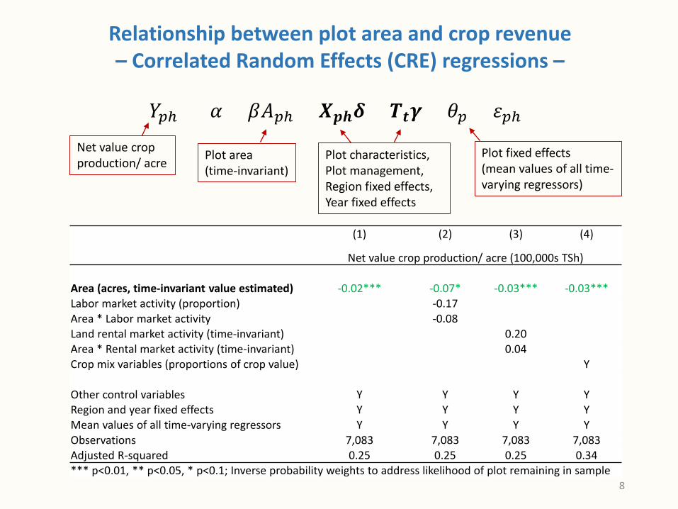
Relationship between plot area and crop revenue – Correlated Random Effects (CRE) regressions –

𝑌𝑌𝑝𝑝𝑝 = 𝛼𝛼 + 𝛽𝛽𝐴𝐴𝑝𝑝𝑝 + 𝑿𝑿𝒑𝒑𝒑𝒑𝜹𝜹 + 𝑻𝑻𝒕𝒕𝜸𝜸 + 𝜃𝜃𝑝𝑝 + 𝜀𝜀𝑝𝑝𝑝Net value crop production/ acre Plot area

(time-invariant)Plot characteristics,Plot management,Region fixed effects,Year fixed effects

Plot fixed effects (mean values of all time-varying regressors)

(1) (2) (3) (4)

Net value crop production/ acre (100,000s TSh)

Area (acres, time-invariant value estimated) -0.02*** -0.07* -0.03*** -0.03***Labor market activity (proportion) -0.17Area * Labor market activity -0.08Land rental market activity (time-invariant) 0.20Area * Rental market activity (time-invariant) 0.04Crop mix variables (proportions of crop value) Y

Other control variables Y Y Y YRegion and year fixed effects Y Y Y YMean values of all time-varying regressors Y Y Y YObservations 7,083 7,083 7,083 7,083Adjusted R-squared 0.25 0.25 0.25 0.34*** p<0.01, ** p<0.05, * p<0.1; Inverse probability weights to address likelihood of plot remaining in sample

8

Preliminary Conclusions

• IR is persistent in plot-level analysis.

• IR evident along spectrum of plot sizes.

• Pooled OLS indicates IR intensity is at least partially correlated with local levels of labor and land market activity. However, this relationship does not seem to persist in a CRE analysis.

• Crop mix, unobserved plot effects do not seem to (fully) explain the IR

What’s next?

• Treatment of plot measurement error• Further consideration of heterogeneity along plot size spectrum

(e.g., market activity interactions)

9

(1) (2) (3) (4) (5)Dependent variable: Net value crop production/ acre

(100,000s TSh)Area (acres, estimated) -0.05*** -0.10*** -0.04*** -0.02*** -0.009Area2 0.0004***

Control variables Y Y Y

Region and Year Fixed Effects Y Y

Household-Year Fixed Effects YSlope on area=0 at this value: 124.74 acres% Plots larger than this value: 0.03%Observations 15,493 15,493 15,493 15,493 12,829*** p<0.01, ** p<0.05, * p<0.1

Pooled OLS from slide #2 (with all plots including those > 50 acres)

(1) (2) (3) (4) (5)Dependent variable: Net value crop production/ acre

(100,000s TSh)Area (acres, estimated) -0.04*** -0.08*** -0.03*** -0.02*** -0.01Area2 0.0003***

Control variables Y Y Y

Region and Year Fixed Effects Y Y

Household-Year Fixed Effects YObservations 13,635 13,635 13,635 13,635 11,214*** p<0.01, ** p<0.05, * p<0.1

Pooled OLS from slide #2 (excluding plots < 0.5 acres)

10

(1) (2) (3) (4) (5) (6)Dependent variable: Net value crop production/ acre (100,000s TSh)

Area (acres, estimated) -0.02*** -0.01 -0.02*** -0.01 -0.02*** -0.02**

Labor market activity (proportion) 0.003 -0.05

Area * Labor market activity -0.02Land market activity 1.00*** 1.04***

Area * Land market activity -0.01Land rental market activity 0.90** 0.85**

Area * Rental market activity 0.02Other control variables Y Y Y Y Y YRegion and year fixed effects Y Y Y Y Y YSlope on area=0 at market activity level: N/A N/A 0.55% Households beyond this point 2.78%

From slide #4 (excluding plots < 0.5 acres)

11

Thank you

13

Percent of cropping households that rented/ borrowed a tractor (left) or used a tractor (right)

Relationship between area planted and crop yield(specific crops, Agricultural Sample Census 2008/09)

14

ObservationsArea planted (acres)Mean Observations > 20 acres

Maize 29,935 2.27 156Rice 9,139 1.90 32Beans 9,953 1.01 11Households/ Farms (growing crops) 49,502 2,619 (total land held)

Non-parametric polynomial regressions

Relationship between area planted and crop yield(specific crops, Agricultural Sample Census 2008/09)

Non-parametric polynomial regressions, x-axis extends up to 99th percentile

15

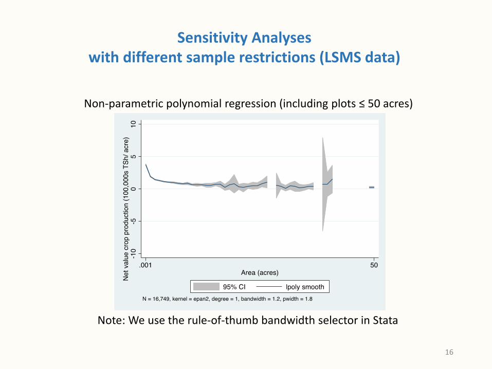
Non-parametric polynomial regression (including plots ≤ 50 acres)

Note: We use the rule-of-thumb bandwidth selector in Stata

Sensitivity Analyseswith different sample restrictions (LSMS data)

16