the environmental protection agency’s budget from 1970 to

The Environmental Protection Agency’s Budgetfrom 1970 to 2010: A Lifecycle Analysis

PETER J. BALINT AND JAMES K. CONANT

Using three approaches, we attempt to explain changes in the EnvironmentalProtection Agency’s operating budget from 1970 to 2010. First, we comparequalitative predictions from two general types of agency lifecycle theories to theactual path of the EPA’s budget. Second, we test empirically several hypothesesregarding the effects of political, economic, and other variables on the agency’sbudget. Third, we conduct detailed historical case studies of selected years. Theresults offer hints of support for theories predicting incremental change but do notsupport the hypothesized effects of external factors. We also uncover some historicalanomalies that warrant further research.

INTRODUCTION

The official birth date of the U.S. Environmental Protection Agency is December 2, 1970. On

that date, President Nixon’s nominee to be the administrator of the new agency, William

Ruckelshaus, was confirmed by the Senate, and the “EPA opened for business in a tiny suite of

offices at 20th and L Streets in Northwest Washington, D.C.” (Lewis 1985, 1). The birth of the

new agency was set in motion when President Nixon submitted Reorganization Plan No. 3 to

Congress on July 9, 1970. As part of this plan, programs and offices operating in the Department

of Health, Education, and Welfare, the Department of the Interior, the Department of

Agriculture, the Food and Drug Administration, the Atomic Energy Commission, and the

Federal Radiation Council were to be combined in the new Environmental Protection Agency.

In this article, we examine and attempt to explain what has happened to this major regulatory

agency over the 40-year period from its birth in 1970 to 2010. In examining the history of the

EPA, we apply qualitative and quantitative methods to test hypotheses that follow from two

Peter J. Balint is an Associate Professor in the Department of Public and International Affairs at George Mason

University, Fairfax, VA. He can be reached at [email protected].

James K. Conant is a Professor in the Department of Public and International Affairs at George Mason University,

Fairfax, VA. He can be reached at [email protected].

© 2013 Public Financial Publications, Inc.

22 Public Budgeting & Finance / Winter 2013

broad categories of theoretical agency lifecycle models found in the political science and public

administration literature. The first category of theoretical agency lifecycle models we consider

proposes that the changes mature federal agencies experience in their vitality and influence over

time are generally incremental, and that these incremental changes have an internal momentum

apparently unaffected by outside influences (Davis, Dempster, and Wildavsky 1966, 1974). In

contrast, the second category of theoretical agency lifecycle models proposes that the vitality and

influence of agencies vary in response to external drivers, such as partisan political factors,

economic conditions, public attitudes, triggering events, and so forth (for a review, see Auten,

Bozeman, and Cline 1984).

In the case of the EPA, our principal indicator of the agency’s vitality and influence is its

operating budget, which includes core activities such as research, regulation, enforcement, and

facilities management, but excludes expenditures for Superfund and for grants or revolving fund

outlays to states, municipalities, and tribes. In measuring the EPA’s budget in this way, we

follow the lead of other scholars who have studied the agency (e.g., Vig and Kraft 2013).1

Throughout, when discussing budgets in particular years we are referring to fiscal years.

We attempt to explain changes in the EPA’s operating budget using three approaches. First,

we predict general development paths for the agency following from the two categories of

theoretical models introduced above, and then offer qualitative assessments of the fit of the

observed trajectory of the EPA to the paths predicted by the theories. Second, we present and

interpret the results of regression analyses in which we examine hypothesized relationships

between trends for the EPA’s budget and changes in various political, economic, and other

variables that can be expected to influence the agency’s budget under externally driven theories.

Third, we supplement these qualitative and quantitative assessments of the overall 40-year life

history of the EPA with more narrowly focused case studies of selected fiscal years in which the

EPA experienced unusually large changes in its budget, either positive or negative, compared to

the years immediately prior. Before reviewing the predictions of the theoretical models and

describing the results of our empirical analyses, we begin with a brief review of the historical

context for the establishment of the EPA.

HISTORICAL CONTEXT

The year 1970 has been described as the “year of the environment” (Lewis 1985, 1). On

January 1, 1970, President Nixon signed into law the National Environmental Policy Act

1. The EPA budget data used in this study are from the annual presidents’ budgets. Accessed May 7, 2013. http://

fraser.stlouisfed.org/publication/?pid¼54. Each year, the president’s budget contains proposed budgetary authority

for all agencies for the upcoming fiscal year, estimates for the current year and immediate prior year, and actual

values for the year two years prior. In compiling our dataset, we used the actual budget for each fiscal year as reported

in the president’s budget from two years following. Thus, to ensure comparable numbers from a consistent source,

the most recent year in our dataset is FY 2010, taken from the FY 2012 budget. In adjusting for inflation, we used the

CPI inflation calculator of the Department of Labor, Bureau of Labor Statistics. Accessed May 7, 2013. http://www.

bls.gov/data/inflation_calculator.htm

Balint and Conant / The Environmental Protection Agency’s Budget from 1970 to 2010 23

http://www2.epa.gov/aboutepa/birth-epa



http://www.presidency.ucsb.edu/ws/?pid&x003D;2921


(NEPA). In that law, Congress articulated for the first time a national policy on the environment.

The president used his State of the Union address on January 22 to propose making “the 1970s an

historic period when, by conscious choice, we transform our land into what we want it to

become” (Nixon 1970a). On April 15, the president’s Committee on Executive Branch

Organization, known as the Ash Committee, submitted its report, which included a

recommendation for establishing a new environmental protection agency.

The Ash Committee’s recommendation gained momentum on April 22, when millions of

people across the country participated in the first Earth Day celebration. On July 7, the president

submitted to the House of Representatives his Reorganization Plan No. 3, the core element of

which was the creation of the EPA. By declining to oppose this plan, Congress signaled its

favorable response, and the EPA opened for business on December 2. On December 31, 1970, to

cap off the “year of the environment,” President Nixon signed into law a major new revision of

the Clean Air Act passed by Congress.

In establishing the EPA, President Nixon acknowledged that he was making an exception to

one of his key principles, that “as amatter of effective and orderly administration, additional new

independent agencies normally should not be created” (Nixon 1970b, 205). Among the reasons

the president offered for overriding this principle was that “concern with the condition of our

physical environment has intensified” (Nixon 1970b, 203). This comment revealed a political

sensitivity to both emerging public activism on the environment and the energetic way in which

Congress was developing new environmental legislation (Agnone 2007). Part of the president’s

motivation in promoting his environmental agenda was to co-opt an issue that might otherwise

have served as a strong platform for potential Democratic presidential challengers in the

upcoming elections of 1972 (Kraft and Vig 2013).

Two other reasons President Nixon offered for his actions were long established and widely

accepted arguments for executive branch reorganization. He wrote that, “Government’s

environmentally related activities have grown up piecemeal over the years,” and that the time

had “come to organize” those activities “rationally and systematically” (Nixon 1970b, 203). In

particular, the president asserted that, “As no disjointed array of separate programs can, the EPA

would be able—in concert with the States—to set and enforce standards for air and water quality

and for individual pollutants” (Nixon 1970b, 205).

The EPA was created in a time of high public concern for the environment and broad

bipartisan support in government for strong new regulations to protect the environment and

promote public health. Over the course of the next 40 years, however, public and congressional

support for the agency waxed and waned. By the early 1980s, strongly polarized attitudes

towards environmental protection in general, and the EPA in particular, had replaced the

favorable bipartisan consensus of the 1970s. During some periods, including the late 1980s and

early 1990s, a measure of broad support reemerged, but at other times, including the recent 2012

election cycle, polarization has returned and partisan attacks on the EPA as a “job-killer” have

intensified (e.g., Young 2012). As noted in the agency’s history reported on the EPA’s own

website, “Few federal agencies evoke as much emotion in the average American as the U.S.

Environmental Protection Agency” (Williams 1993, 1).


GENERAL QUALITATIVE PREDICTIONS FROM AGENCY

LIFECYCLE THEORIES

As noted earlier, we use two categories of theoretical agency lifecycle models to frame this

study: those that predict agency trajectories will change incrementally following an internal

momentum and those that predict agency trajectories will be shaped by the effects of external

forces. In considering these two general theoretical models, we apply a concrete example for

each (see also Conant and Balint 2011). As an example of incremental, internally driven

models, we use Anthony Downs’s (1967) biological model for the growth and development of

organizations. As an example of externally driven models, we use the partisan political

model.

In his model, Downs proposed that human organizations, like living organisms, are born,

grow, age, and (perhaps) die. He identified various processes by which organizations are born,

but he contended that newborn agencies, like newborn biological life forms, face risks of

infant mortality, particularly from the attacks of competitors. He argued, however, that once

an agency passes through an “initial survival threshold” (Downs 1967, 9, emphasis in

original) and reaches maturity, it may live more or less indefinitely, gradually losing its

energy and entrepreneurial spirit but maintaining its size and concern for protecting its

domain. While we briefly discuss the EPA’s startup stage below, it is the long-lasting, mature

stage of the biological theory of agency lifecycles that we use as an example of the class of

incremental theories of agency progression.

The partisan political model serves as an example of externally driven theories of agency

trajectories. The primary assumption is that the level of support an agency receives, and thus its

vitality or even survival, depends on whether its function aligns with the priorities of the party

in power. Following this logic, a president and Congress supportive of an agency’s mission

will increase its budget and nominate and confirm political appointees with similar views to

leadership positions. Conversely, an agency that focuses on issues devalued by a president and

Congress is likely to be led by hostile political appointees and endure budgetary

malnourishment or starvation. The model predicts that these effects will be strongest when

the White House and Congress are controlled by the same party and tempered when political

power is divided.

Using the biological model to make a rough qualitative prediction of the EPA’s budgetary

history, we would expect to see rapid growth in the early years, at least until the agency passed

through the “initial survival threshold.” Then, we would expect to see an extended period of

relative stability characterized by incremental changes to an established base. In contrast, if we

use the partisan political model as the basis for a rough qualitative prediction, wewould expect to

see a more contingent, wavelike path for the EPA’s budget. Given the stereotypical ideologies of

the two parties in this simple model, we would expect to see a pattern of increases during periods

of Democratic Party ascendancy and declines during periods of Republican Party ascendancy.

Recognizing the increased polarization of the parties that began with the election of Ronald

Reagan in 1980, we would expect shifts in party control in Washington to generate greater

variation in the EPA’s budget since that time.


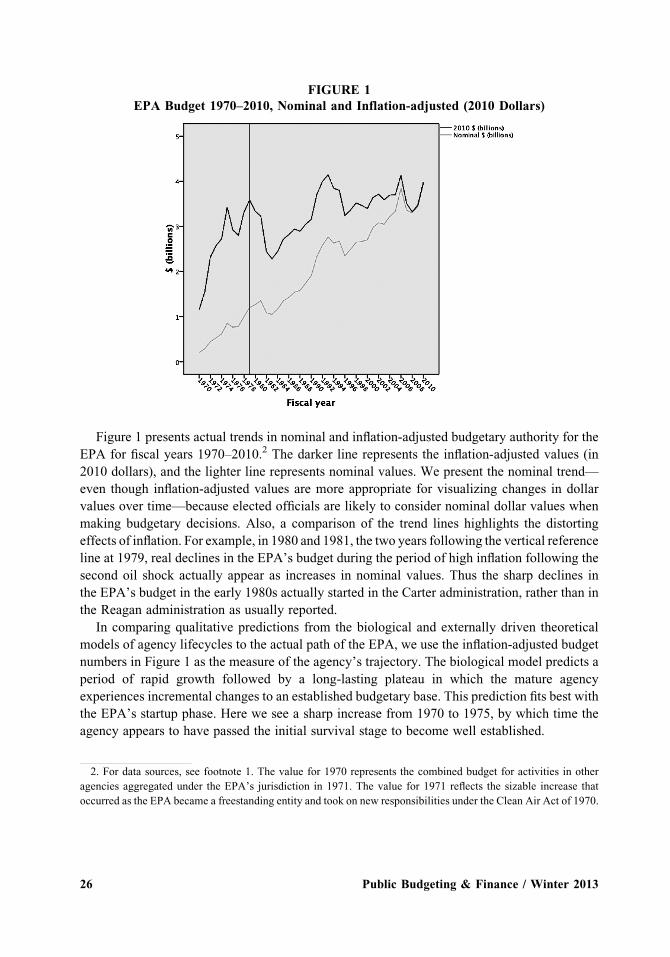
Figure 1 presents actual trends in nominal and inflation-adjusted budgetary authority for the

EPA for fiscal years 1970–2010.2 The darker line represents the inflation-adjusted values (in

2010 dollars), and the lighter line represents nominal values. We present the nominal trend—

even though inflation-adjusted values are more appropriate for visualizing changes in dollar

values over time—because elected officials are likely to consider nominal dollar values when

making budgetary decisions. Also, a comparison of the trend lines highlights the distorting

effects of inflation. For example, in 1980 and 1981, the two years following the vertical reference

line at 1979, real declines in the EPA’s budget during the period of high inflation following the

second oil shock actually appear as increases in nominal values. Thus the sharp declines in

the EPA’s budget in the early 1980s actually started in the Carter administration, rather than in

the Reagan administration as usually reported.

In comparing qualitative predictions from the biological and externally driven theoretical

models of agency lifecycles to the actual path of the EPA, we use the inflation-adjusted budget

numbers in Figure 1 as the measure of the agency’s trajectory. The biological model predicts a

period of rapid growth followed by a long-lasting plateau in which the mature agency

experiences incremental changes to an established budgetary base. This prediction fits best with

the EPA’s startup phase. Here we see a sharp increase from 1970 to 1975, by which time the

agency appears to have passed the initial survival stage to become well established.

FIGURE 1

EPA Budget 1970–2010, Nominal and Inflation-adjusted (2010 Dollars)

2. For data sources, see footnote 1. The value for 1970 represents the combined budget for activities in other

agencies aggregated under the EPA’s jurisdiction in 1971. The value for 1971 reflects the sizable increase that

occurred as the EPA became a freestanding entity and took on new responsibilities under the Clean Air Act of 1970.


The years from 1975 to 2010 can be seen overall as a period of slow growth, with the

inflation-adjusted budget in 2010 only 16 percent higher than in 1975. However, the

intermediate changes over this period were hardly incremental and rarely resembled a relatively

flat plateau. In real terms, the EPA’s budget dropped by approximately 35 percent from 1979 to

1983. It then rose 80 percent in 10 years of strong growth to a high point in 1993, before

dropping back by more than 20 percent over the next three years. Despite an increasing

workload, the agency’s budget was about 4 percent lower in 2010 than at its peak in 1993. The

mature stage of Downs’s biological model, or any other incremental model, fails to capture this

volatility.

The partisan political model, in contrast, assumes volatility. It predicts that the EPA’s budget

will rise in times of Democratic Party control and fall in times of Republican Party control. There

are several periods in which this model appears to capture the observed variations. For example,

the agency’s budget rose in the early years of the Carter, Clinton, andObama administrations and

fell during early years of the Reagan administration. Moreover, the decline in the middle of

President Clinton’s first term coincided with the Gingrich revolution in which Republicans

gained control of the House of Representatives for the first time in 40 years. William

Ruckelshaus, writing during this time, used the analogy for the EPA’s budget of a pendulum

swinging back and forth, with each swing representing a backlash to the previous period of pro-

or antiregulatory fervor (Ruckelshaus 1996).

On the other hand, several periods do not match well with the predictions of the political

model. The years of strongest growth for the agency occurred under Republican presidents

Nixon, Ford, and George H. W. Bush. Even during parts of the Reagan and George W. Bush

administrations the agency fared better than might be expected. In the first two fiscal years of

the Reagan administration, 1982 and 1983, the EPA’s budget declined dramatically. In 1983,

however, EPA Administrator Gorsuch resigned under pressure after being cited for contempt

of Congress. Following this period of turmoil, William Ruckelshaus returned to the EPA’s top

position, and the agency’s inflation-adjusted budget increased in five of the remaining six

years of the Reagan administration. During the George W. Bush administration the EPA’s

inflation-adjusted budget was relatively stable with an overall increase over the first five fiscal

years, 2002 through 2006, before experiencing more volatility later in the president’s second

term.

Thus, on the basis of these initial qualitative assessments, it appears that predictions generated

from the two types of theoretical agency lifecycle models do not hold up well in the case of the

EPA. Neither the biological model nor the partisan political model captures a majority of the

variations in the EPA’s budget over time.

QUANTITATIVE ANALYSIS

In this section, we present the results of our efforts to test the theories more rigorously. Although

the findings from our quantitative analysis also turn out to be generally inconclusive, we discuss

some implications of our results for the agency lifecycle theories.


Dependent Variable

Figure 2 presents data for inflation-adjusted EPA budgetary authority from 1973 to 2010 in the

form of percent change from the previous year.3 A bar above the zero line indicates a positive

change in the EPA’s budget, and a bar below the zero line indicates a negative change. In

building our statistical models, we used the data presented in Figure 2 as the dependent variable.

Using the transformation of the data to “percent change from the previous year” from the

inflation-adjusted dollar values presented in Figure 1 has two benefits. The first is

methodological, in that it minimizes the adverse effects on regression results of inflationary

and noninflationary growth over time and the associated autocorrelation of the error terms. The

second is conceptual, in that what we actually want to explain is the change in budgetary

authority from one year to the next, rather than the dollar value of the budget in a given year.

Summary statistics for the selected form of the dependent variable indicate that the mean

percent change from the previous fiscal year in the inflation-adjusted budget for the EPA isþ1.9

percent. While the distribution is approximately normal, the standard deviation of 9.96 percent

indicates a high degree of variation. The maximum annual increase is 26 percent in 1975

(z¼ 2.4), and the maximum decrease is 24 percent in 1982 (z¼�2.6). While these are the only

FIGURE 2

EPA Budget 1973–2010, Percent Change from Previous Year (Inflation-adjusted)

3. 1970 and 1971 are omitted because the EPA was established during FY 1971; 1972 is omitted because in

measuring the variable as the change from one year to the next there is no value for the first year in the series.


two values more than two standard deviations from the mean, there are six other years in which

the annual change is 15 percent or greater, either positive or negative.

Explanatory Variables

Following other researchers (Bozeman 1977; Kiewiet and McCubbins 1988; Wlezien

1995, 2004) and drawing from the agency lifecycle theories described above, we examined

various political, economic, and social indicators as potential explanatory variables. The

political variables focus on the federal legislative and executive branches. In building our

regression models, we experimented with various combinations of variables measuring party

control of the presidency and party membership in, and control of, each house of Congress.4 We

also tested interaction variables for these indicators. Political variables presented in our

regression results below include Democrats in the House as a percent of total membership and a

dummy variable capturing whether the president was a Democrat or Republican. For economic

variables, we tested the unemployment rate and the rate of growth or decline in gross domestic

product (GDP). In models presented below, we show results for the GDP variable.5 While we

experimented with lagged and nonlagged values for the political and economic variables,

lagging these variables by one year is appropriate as budgets for a given fiscal year are

established in the prior year.

We tested two other explanatory variables: public opinion regarding spending on the

environment, and overall federal nondefense spending. For the public opinion variable, we used

responses to a question included in the General Social Survey asking respondents whether they

think the country is spending “too much,” “too little,” or “about the right amount” on the

environment.6 This question was asked in the survey for 27 of the 38 years from 1973 to 2010

used in our analysis.7 Following Wlezien (2004), we included this variable as net public support

for more spending on the environment, computed by subtracting the percent responding “too

much” from the percent responding “too little.” This variable was also lagged by one year.

4. Party makeup of Congress is drawn from the websites of the House and Senate. Accessed May 7, 2013. http://

history.house.gov/Institution/Party-Divisions/Party-Divisions/

5. GDP data are from the Department of Commerce, Bureau of Economic Analysis,National Income and Product

Accounts Tables, Table 1.1.1. Accessed May 7, 2013. http://www.bea.gov/iTable/iTable.cfm?ReqID¼9&

step¼1#reqid¼9&step¼1&isuri¼1

6. The data and codebook are available from the General Social Survey website. Accessed May 7, 2013. http://

www3.norc.org/GSSþWebsite/. The question reads: “We are faced with many problems in this country, none of

which can be solved easily or inexpensively. I’m going to name some of these problems, and for each one I’d like you

to tell me whether you think we’re spending too much money on it, too little money, or about the right amount.

First… arewe spending toomuch, too little, or about the right amount on…?” From1973 to 1983, the environmental

item was worded “…improving and protecting the environment.” Beginning in 1984, for some respondents, these

words were replaced with simply “…the environment.” Following Dunlap and Scarce (1991), we combine responses

for years in which both versions were asked.

7. The question appeared on the General Social Survey in all years from 1973 to 1994, except 1979, 1981, and

1992. From 1994 to 2010, the question was asked only in even-numbered years. Because we lag this variable by one

year in our models, we also lose the value for 1973, leading to n¼ 26 for regressions including this variable.


Wlezien (1995) suggests that public opinion can act as a “thermostat,” moderating budgetary

fluctuations. That is, greater public willingness to spend money on a salient policy issue induces

policymakers to increase appropriations in that area. Then as spending rises, public pressure for

additional expenditures in that policy realmwanes, discouraging further increases. In this model,

public opinion on spending in a policy area and actual appropriations in that area affect each

other in a cyclical manner, tending to maintain relative budgetary stability. In our research, we

focused on the first part of this cycle—the impact of a change in net public support for more

environmental spending on the EPA’s budget in the following fiscal year.

The overall federal nondefense spending variable was measured as percent change from the

previous year.8Wlezien’s research also provides support for including this variable. He finds that

social policy areas may be aggregated in theminds of voters and their elected representatives. He

writes that policymakers in making budgets may “respond to a general preference for

government action broadly defined, in effect, across various policy areas,” rather than more

narrowly “to public preferenceswithin particular areas” (Wlezien 2004, 2, emphasis in original).

He finds, for example, that spending preferences for the environment tend to move together with

those for welfare, education, health, and urban issues. He also describes a “guns-butter trade-off”

in which budgetary pressures for social priorities are typically inversely related to movements in

national defense budgets (Wlezien 2004, 7). Thus, we included the nondefense spending

variable, unlagged, to help us explore whether the EPA’s budget tends to moves in tandem with

overall social spending.

Hypotheses

We state the hypotheses for our quantitative analysis in two ways based on the two types of

theoretical agency lifecycle models described earlier. First, we state the hypotheses based on

predictions for changes in the EPA’s budget following fromDowns’s biological model of agency

lifecycles, with particular focus on the mature stage of the lifecycle beyond the initial survival

threshold.9 The mature stage of this model fits in the general class of incremental agency

lifecycle theories, which predict marginal changes over time to a relatively stable budgetary

base. Thesemodels also generally predict that the changes that do occur in the base will follow an

internal momentum apparently independent of external influences.

Next we state the hypotheses based on predictions for changes in agency budgets following

from the partisan political model. This model fits in the general class of agency lifecycle models

that emphasize the effects of forces external to the agency, such as party control of Congress and

the White House, economic conditions, public attitudes, triggering events, and so forth.

8. Federal nondefense spending figures are from the Department of Commerce, Bureau of Economic Analysis,

National Income and Product Accounts Tables, Table 3.10.1. Accessed May 7, 2013. http://www.bea.gov/iTable/

iTable.cfm?ReqID¼9&step¼1#reqid¼9&step¼1&isuri¼1

9. As indicated in footnote 3, data for themeasure of the dependent variable presented in figure 2 do not include the

EPA’s initial startup years. Thus the regression results are most relevant for the mature stage of the biological model.


H1:From the perspective of incremental models: No systematic effect on the EPA’s budget of

changes in party control in the legislative and executive branches. From the perspective of

externally driven models: More Democratic Party control leads to a higher budget for the

EPA.

H2:From the perspective of incremental models: No systematic effect on the EPA’s budget of

changes in GDP. From the perspective of externally driven models: Higher GDP growth

leads to a higher budget for the EPA.

H3:From the perspective of incremental models: No systematic effect of changes in net public

support for more spending on the environment on the EPA’s budget.From the perspective

of externally driven models: An increase in net public support for more spending on the

environment leads to a higher budget for the EPA.

H4: From the perspective of both incremental and externally driven models: The EPA’s

budget will be higher when overall federal nondefense spending is higher. Incremental

models predict that changes to agency budgets may occur in similar ways across

government, apparently independent of external forces. In other words, incremental

changes in overall nondefense spending may reflect a scaling up of incremental changes

at the agency level. Models emphasizing the effects of external factors also predict that

the EPA’s budget will tend to move in tandem with social spending in general. But in

these models, as described above, the theory is that social spending categories tend to be

aggregated in the minds of policymakers and the public, creating external pressure for

budgets in nondefense categories to move together.

Limitations

Two characteristics of the data limit the explanatory power of our statistical models. First, the

dataset has a relatively small number of observations (n¼ 38: the years from 1973 to 2010,

inclusive), and this number is reduced further when public opinion polling is included as several

years of data are missing for this variable. Second, the dependent variable has a large standard

deviation. The small size of the dataset and the large variance in the dependent variable both

work to reduce the likelihood of finding statistical significance.

Results and Discussion for the Regression Models

As the dependent variable, percent change from the previous year in the EPA’s budget, is

continuous, we applied ordinary least squares regression, in the form y¼ aþ b1x1þ b2x2þ…þ e, to examine relationships between the dependent variable (y) and various combinations of

the independent variables (xi) described above.


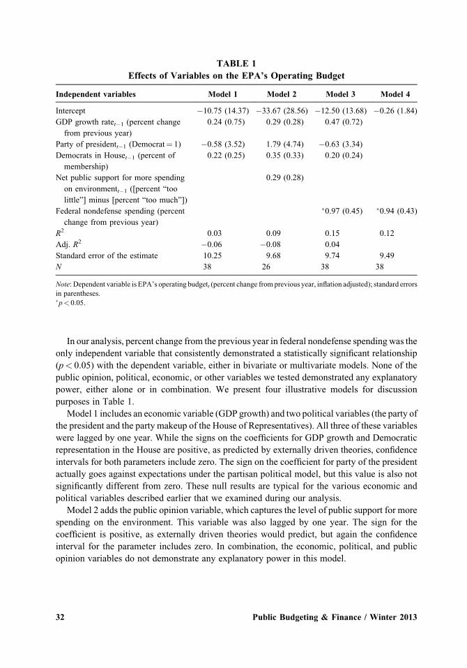
In our analysis, percent change from the previous year in federal nondefense spending was the

only independent variable that consistently demonstrated a statistically significant relationship

(p< 0.05) with the dependent variable, either in bivariate or multivariate models. None of the

public opinion, political, economic, or other variables we tested demonstrated any explanatory

power, either alone or in combination. We present four illustrative models for discussion

purposes in Table 1.

Model 1 includes an economic variable (GDP growth) and two political variables (the party of

the president and the party makeup of the House of Representatives). All three of these variables

were lagged by one year. While the signs on the coefficients for GDP growth and Democratic

representation in the House are positive, as predicted by externally driven theories, confidence

intervals for both parameters include zero. The sign on the coefficient for party of the president

actually goes against expectations under the partisan political model, but this value is also not

significantly different from zero. These null results are typical for the various economic and

political variables described earlier that we examined during our analysis.

Model 2 adds the public opinion variable, which captures the level of public support for more

spending on the environment. This variable was also lagged by one year. The sign for the

coefficient is positive, as externally driven theories would predict, but again the confidence

interval for the parameter includes zero. In combination, the economic, political, and public

opinion variables do not demonstrate any explanatory power in this model.

TABLE 1

Effects of Variables on the EPA’s Operating Budget

Independent variables Model 1 Model 2 Model 3 Model 4

Intercept �10.75 (14.37) �33.67 (28.56) �12.50 (13.68) �0.26 (1.84)

GDP growth ratet�1 (percent change

from previous year)

0.24 (0.75) 0.29 (0.28) 0.47 (0.72)

Party of presidentt�1 (Democrat¼ 1) �0.58 (3.52) 1.79 (4.74) �0.63 (3.34)

Democrats in Houset�1 (percent of

membership)

0.22 (0.25) 0.35 (0.33) 0.20 (0.24)

Net public support for more spending

on environmentt�1 ([percent “too

little”] minus [percent “too much”])

0.29 (0.28)

Federal nondefense spending (percent

change from previous year)

�0.97 (0.45) �0.94 (0.43)

R2 0.03 0.09 0.15 0.12

Adj. R2 �0.06 �0.08 0.04

Standard error of the estimate 10.25 9.68 9.74 9.49

N 38 26 38 38

Note: Dependent variable is EPA’s operating budgett (percent change from previous year, inflation adjusted); standard errors

in parentheses.�p< 0.05.


Models 3 and 4 include the federal nondefense spending variable. Model 3 retains the

economic and political variables, while model 4 shows the simple bivariate relationship between

federal nondefense spending and the EPA’s budget. The coefficient for the nondefense spending

variable is stable and statistically significant (p< 0.05) across the two models. The effect size is

also notable, in that these twomodels predict that on average themagnitude of the annual percent

change in the EPA’s budget from the prior year will be approximately the same as that for federal

nondefense spending. That is, a one percentage point increase (decrease) in the nondefense

spending variable is associated, on average, with approximately a 0.95 percentage point increase

(decrease) for the EPA’s budget. However, the low R2 values indicate that there remains a high

level of unexplained variation around this average.

Overall, these results fail to support the hypotheses presented in H1, H2, and H3 following

from theoretical models emphasizing the effects of external factors. In our analyses, party

strength in Washington, national economic conditions, and net public support for more

spending on the environment demonstrated no significant impact on annual changes in the

EPA’s budget.

These null results for H1, H2, and H3 hint at support for incremental theories. Annual changes

in the inflation-adjusted budget for the EPA appear to move arbitrarily over time, unaffected in

any systematic way by party ascendancy, economic conditions, or public opinion regarding

spending on environmental protection. Moreover, as described earlier, the percent change in the

inflation-adjusted budget over the previous year for the 38-year period averages a modest,

incremental 1.9 percent increase. In eight out of the 38 years, however, the percent change from

the previous year, positive or negative, was 15 percent or greater. Relatively frequent shifts of

this magnitude conflict with theories predicting incremental changes.

The results support H4, as models 3 and 4 in Table 1 show a positive correlation between the

EPA’s budget and federal nondefense spending more broadly. As noted in the statement of the

hypothesis, incremental and externally driven theories both predict that the agency’s budget will

tend to move in the same direction as overall nondefense spending. However, the evidence here

is stronger for the incremental, internally driven interpretation because the posited drivers in the

externally driven theory—the public opinion, economic, and political variables—show no

relationship with the EPA’s budget in model 2.10 However, we do not make strong claims for this

finding. The regression models including the nondefense spending variable have limited

explanatory power and are unable to account for the considerable swings in the EPA’s budget

over the period of our study.

The caveats mentioned earlier also limit the value of the null results for H1, H2, and H3. The

dataset is relatively small and there is a high level of variation in the dependent variable. These

characteristics increase the risk of type 2 errors, in which the analysis fails to detect real effects of

independent variables on the dependent variable. Thus, the results hinting at support for

incremental theories, while suggestive, are inconclusive.

10. Repeating model 2 with nondefense spending as the dependent variable also produces insignificant results

(F¼ 0.28; p¼ 0.89).


HISTORICAL CASE STUDIES

In the previous section, we emphasized that the variation in the dependent variable—the yearly

change in the EPA’s budget—limited the power of the regression analysis. In this section, we

explore the sources of this wide variation by looking more closely at the fiscal years in which the

change in the EPA’s operating budget from the previous year was greater than 15 percent,

positive or negative: 1975, 1976, 1978, 1982, 1991, 1996, 2007, and 2010.11

To narrow our examination of these case study years, we focus on the gap for each year

between the president’s budget request and the actual budgetary authority granted by

Congress.12 Then, to explore finer-grained differences in priorities between the president and

Congress, we examine changes in the accounts within the annual budget. In examining the case

study years, we also consider the effects of party control in Congress and theWhite House during

these years. Finally, at the end of the section, we discuss the increase of 11 percent in 2006, which

is of interest because it reflects a large, unexplained, single-year spike in one budget account.

Overview of Presidential and Congressional Budgetary Support for the EPA

To prepare for the examination of the gap between presidential budgetary requests for the EPA

and the actual congressional budgetary authority granted to the agency in the case study years,

we first review the gap as it varied over the entire period of our study. Figure 3 presents the trends

in nominal dollars. The lighter line represents presidential budgetary requests and the darker line

represents congressional budgetary authority granted.

Figure 4 displays the gap in percentage terms. A bar extending above the zero line in Figure 4

indicates that Congress granted more funding for the EPA in that year than the president

requested. A bar extending below the zero line indicates that Congress granted less funding for

the EPA in that year than the president requested.

These two figures demonstrate that Congress has generally been more generous towards the

EPA than presidents have been.13 Bars extend above the zero line for 29 of the 39 years in

Figure 4, and the darker line is above the lighter line in Figure 3 for a commensurate number of

years. The presentation in percentage terms allows for clearer comparisons of the size of the gap

over time. For example, the gaps illustrated in Figure 4 generally appear larger in the earlier years

than they do in Figure 3, as compared to later years. This distortion results from the increasing

size over time of the baseline budget in nominal dollars.

Several of the case study years listed at the beginning of this section stand out in Figures 3

and 4 while others do not. Figure 4 highlights the striking gaps in 1982 and 1996, when Congress

provided substantially less funding for the EPA than the presidents requested. Figure 3 shows the

11. To avoid distortions from the early period of rapid budgetary growth, we omit 1971 and 1972.

12. For discussion of budgetary competition between the president and Congress, see, e.g., Kiewiet andMcCubbins

(1985); Wlezien and Soroka (2003); and Canes-Wrone, Howell, and Lewis (2008).

13. Figure 4 presents data for 39 years, from 1972 to 2010, inclusive. The president did not make official budget

proposals for the EPA in FY 1970 or 1971 because the agency was not formally established until December 1970,

when FY 1971 was already underway.


spike in budget authority granted by Congress in 2006 compared to the president’s request in that

year. The case study years that do not stand out in Figures 3 and 4 are those in which the president

and Congress generally agreed on the cuts to or increases in the EPA’s budget.

A Comparison of Presidential and Congressional Budgetary Support in Case Study Years

Table 2 presents detailed information for the eight case study years of the EPA’s budget, those

with changes of 15 percent or more, positive or negative, from the years immediately prior. For

these years, the table summarizes presidential budgetary requests, congressional budgetary

authority granted, and the difference between them, both by overall agency budget and by

account within the budget.

Because in these case studies we compare numbers within years rather than across years, the

figures for the presidential budgetary requests and the budgetary authority granted by Congress

are nominal, reflecting the actual amounts in the budget documents for those years. The left hand

column of the table identifies the fiscal year, the percent change from the previous fiscal year in

inflation-adjusted budgetary authority (the case study selection criterion), and party control of

Congress and the White House in the prior calendar year when the budget for the fiscal year was

determined.

Table 2 indicates that in three of the four years for which there were large budgetary increases

compared to the previous year (1975, 1978, and 1991), Congress provided substantially higher

budgetary authority than the presidents requested (22 percent higher in 1975, 24 percent higher

FIGURE 3

Presidential Budget Requests and Congressional Budget Authority Granted


in 1978, and 8 percent higher in 1991). Even in the fourth of these years with a large increase

(2010), Congress was slightly more generous than the president (1 percent higher).

In two of the four years in which there were large budgetary decreases compared to the

previous year (1976, 1982, 1996, and 2007), Congress acted to limit the size of the decrease by

adding back some budgetary authority compared to the presidents’ requests (4 percent more than

requested by the president in 1976 and 3 percent more in 2007), although the budgetary authority

granted in these years was still sharply lower than the prior years. In the other two years,

however, Congress took the lead in driving the budget reduction (providing 21 percent less than

the president’s budget request in 1982 and 32 percent less in 1996).

Thus for six of the eight case study years with changes in the EPA’s budget from the prior year of

15 percent or greater, Congress was more generous towards the agency than was the president. This

matches the overall pattern revealed in Figures 3 and 4. Congress has given the EPA a higher budget

than that proposed by the president in about three-quarters of the years from the agency’s

establishment through 2010, and this trend has held in the years of highest budgetary volatility aswell.

The President, Congress, and the Accounts within the Annual Budgets

The data in Table 2 also reveal differing priorities for the president and Congress beyond

disagreements over the agency’s total budget in many of the case study years. For example,

Congress in 1975 substantially increased budgetary authority for the core function of pollution

abatement and control. In that year, Congress also created a new account titled Energy Research

FIGURE 4

Percent the Budget Authority Granted by Congress is Greater Than (Bars above Zero) or

Less Than (Bars below Zero) the President’s Budget Request


TABLE 2

Accounts within EPA Budget (Millions):

Proposed by President versus Approved by Congress

Year Account President Congress % Difference

1975 (þ26% from prior year) Abatement & Control 408 437 7.1

Ford (R) Research & Development 171 167 �2.7

House (D) Energy Research & Development 0 134 N/A

Senate (D) Agency & Regional Management 59 60 2.6

Enforcement 53 51 �4.2

Building & Facilities 0 2 N/A

Total 695 850 22.3

1976 (�15%) Abatement & Control 340 375 10.5

Ford (R) Research & Development 163 265 62.4

House (D) Energy Research & Development 112 0 �100

Senate (D) Agency & Regional Management 656 72 9.0

Enforcement 54 52 �3.0

Building & Facilities 2 3 41.4

Total 743 772 3.9

1978 (þ18%) Agency & Regional Management 72 83 15.2

Carter (D) Research & Development 261 317 21.4

House (D) Abatement & Control 395 521 32.0

Senate (D) Enforcement 68 74 7.2

Buildings & Facilities 1 0 �100

Total 803 999 24.4

1982 (�24%) Salaries & Expenses 646 555 �14.0

Reagan (R) Research & Development 229 154 �32.7

House (D) Abatement, Control, & Compliance 492 373 �24.2

Senate (R) Buildings & Facilities 6 4 �45.5

Total 1,376 1,086 �21.1

1991 (þ18%) Salaries & Expenses 1,000 994 �0.6

GHW Bush (R) Research & Development 249 260 4.2

House (D) Abatement, Control, & Compliance 865 979 13.1

Senate (D) Buildings & Facilities 13 40 207.7

Total 2,127 2,300 8.1

1996 (�15%) Program & Research Operations 1,042 0 �100

Clinton (D) Research & Development 477 0 �100

House (R) Science & Technology 0 540 N/A

Senate (R) Buildings & Facilities 113 110 �2.5

Abatement, Control, & Compliance 1,809 0 �100

Environmental Programs & Management 0 1,697 N/A

Total 3,441 2,347 �31.8

2007 (�15%) Science & Technology 834 769 �7.8

GW Bush (R) Environmental Programs & Management 2,392 2,554 6.8

House (R) Buildings & Facilities 40 40 0

Senate (R) Total 3,266 3,363 3.0

(continued)


and Development and provided funding not requested by the president. In 1976, in a turnabout,

the president requested money for the Energy Research and Development account, but Congress

eliminated it, possibly in anticipation of the creation of the Department of Energy, which

occurred in 1977. However, Congress in 1976 did allocate substantially more funding than

requested by the president for research and development.

In 1982, Congress implemented cuts across the board that were deeper than those included in

the president’s budget, but legislators put particularly strong emphasis on reducing the accounts

for research and development and for abatement, control, and compliance. In 1991, Congress

chose to provide three times as much as the president requested for buildings and facilities. In

1996, Congress not only cut the agency’s overall budget, but also significantly reconfigured the

accounts within the budget.

The frequent shifts described in this section reflect ongoing tensions between the priorities of

presidents and Congress. These changes in accounts within the annual budget have destabilizing

effects on the agency independent of overall changes in the total budget (Ruckelshaus 1996).

The Impact of Party Control on the EPA’s Budget in the Case Study Years

The data in Table 2 show that all four years of major budgetary increases for the EPA occurred

when Democrats controlled both the House and Senate (1975, 1978, 1991, and 2010). Yet one of

the years with a major decrease (1976) also occurred when Democrats controlled both houses of

Congress, and one other year with a major decrease occurred when Democrats controlled the

House of Representatives (1982). Two of the four years of major increases for the EPA’s budget

occurred under Republican presidents (1975 and 1991) and two occurred under Democratic

presidents (1978 and 2010). Three of the four years of major decreases occurred under

Republican presidents (1976, 1982, and 2007) and one under a Democratic president (1996).

These inconsistent effects of party control in Congress and the White House help explain why

our regression analyses failed to find significant correlations between political variables and

changes in the EPA’s budget over the time period of our study.

Through the lens of political history, some of these results match expectations and some are

surprising. For example, the sharp reduction in the EPA’s budget in fiscal year 1996 matches

expectations. When Republicans gained control of the House in 1995 for the first time in

40 years, they moved assertively to shrink government, with a particular focus on reducing

TABLE 2 (Continued)

Year Account President Congress % Difference

2010 (þ15%) Science & Technology 842 881 4.6

Obama (D) Environmental Programs & Management 3,024 3,028 0.1

House (D) Buildings & Facilities 37 37 0

Senate (D) Total 3,903 3,946 1.1

Source: Office of Management and Budget, Budget of the United States Government, FY 1972–2012. Washington, D.C.:

Government Printing Office. See footnote 1 for additional details.

Note: Dollar values are nominal; totals may not reflect actual sums of values because of rounding and because some minor

accounts are omitted from the table.


environmental regulations. At the same time, however, President Clinton requested a sizable

increase in the EPA’s budget. Consequently, the data in Table 2 and Figure 4 show that Congress

imposed its deepest cut compared to the president’s request in 1996.

On the other hand, the evidence for 1982 is initially surprising. The generally accepted

narrative for the history of the EPA at this time is that President Reagan drove the sharp cuts in

the agency’s budget, and that Congress attempted to push back against these reductions

(Kraft 2011; Landy, Roberts, and Thomas 1994). The data in Table 2 and Figure 4 for 1982

appear to conflict with this interpretation, as the budget authority granted by Congress in that

year was more than 20 percent lower than the amount requested in the president’s budget. As

Ellwood (1982) reported in an article written at the time, however, the gap between the president

and Congress for fiscal year 1982 is deceiving.

Ellwood describes how “the Reagan administration and its congressional allies sought a

legislative mechanism” to achieve the sharp cuts in federal domestic spending the president

desired. Working with Republicans and conservative Democrats to circumvent the Democratic

leadership in the House, the administration determined that the “reconciliation provisions of the

Congressional Budget Act provided the solution. By putting all the cuts into a single bill, the

advocates of reductions were able to obtain a single vote on the overall magnitude of the

reduction rather than many votes on individual programs” (Ellwood 1982, 50). Thus, for fiscal

year 1982, the Omnibus Budget Reconciliation Act of 1981 more accurately reflected President

Reagan’s wishes than did the president’s budget. During the remainder of the Reagan

administration, as indicated in Figures 3 and 4, Congress did consistently grant higher budgetary

authority for the EPA than requested by the president.

An Anomaly in 2006

Next we briefly discuss the gap for 2006 between the president’s budget request for the agency

and the congressional budget authority granted. Figure 3 shows a spike in the budget authorized

by Congress in that year, while the president’s request followed the general pattern of the

previous several years.

Our examination of accounts within that year’s budget shows that the sharp one-year increase

in 2006 was the consequence of a large and unexplained rise in “offsetting collections,” defined

as proceeds from “business-like transactions” involving the public or other government accounts

(Government Accountability Office 2005). In the case of the EPA, these collections may be fees,

fines, user charges, and so forth. They are listed in the agency’s budget under the Environmental

Programs and Management account.

To give context, offsetting collections were $65 million in 2004, $209 million in 2005, $196

million in 2007, and $138 million in 2008. For 2006, however, the figure was $683million, more

than three times greater than any of the surrounding years.

As we were unable to find any explanation in publicly available documents for this spike, we

contacted budget officials at the EPA. They confirmed our numbers and expressed surprise and

interest in them. But after reviewing their records, they were also unable to explain the

unexpected jump in offsetting collections for 2006.


Limitations

Our case studies of these years with large budgetary variations are necessarily exploratory, rather

than explanatory. The overall patterns in Figures 3 and 4 and the differing priorities revealed in

Table 2 raise questions about the strategies, tactics, and negotiating stances of presidents and

legislators, and the political parties more generally, that these data alone do not allow us to

answer. Next steps would include interviews and archival research to try to understand better the

fine-grained politics behind the large budgetary changes in these years of high volatility.

Results and Discussion for the Historical Case Studies

In looking closely at annual budgets, we found that 74 percent of the time Congress provided

more funding to the EPA than presidents requested. A possible explanation is that Congress feels

stronger ownership of and investment in the agency. Twenty committees in the Senate and 28 in

the House oversee the EPA’s work. Although the agency often frustrates members of Congress,

it remains a source of power and authority for many committee leaders and members.

We also observed substantial, presumably disruptive, year-on-year changes in accounts

within the EPA’s overall budget. Frequently Congress creates accounts, makes sizable changes

to the funding for accounts, or eliminates accounts altogether. This may be a consequence of a

congressional tendency noted by researchers to micromanage the agency (Rosenbaum 2013).

Finally, we discovered two anomalies. The first is the exceptionally large value of $683

million in offsetting collections in the 2006 budget, which as yet remains unexplained. The

second is that, in apparent contradiction with the general understanding of scholars, the president

proposed a higher level of funding for the EPA in 1982 than Congress enacted. This anomaly

appears to be the result of a tactical collaboration between the administration and conservatives

in Congress from both parties.

The findings summarized in this section are intriguing. We anticipate that further research

into these circumstances will reveal useful new information relevant for understanding the

EPA’s budget trajectory.

CONCLUSION

As we learned in our study, the large and irregular fluctuations in the EPA’s budget resist

systematic explanation. These characteristics of the data have direct policy implications as well.

Former EPA Administrator William Ruckelshaus, in his 1996 editorial entitled “Stopping the

Pendulum,” lamented that the exceptional volatility in the EPA’s budget severely undermined

the agency and hampered its effort to achieve its mission.

He wrote that “in the case of environmental policy these violent swings have had an unusually

devastating—perhaps a uniquely devastating—effect on the executive agency entrusted to carry

out whatever environmental policy the nation says it wants” (Ruckelshaus 1996, 229). He added,

using a powerful metaphor, that “The EPA suffers from battered agency syndrome” (emphasis in


original) and implored Congress and the public to “stop the continuous swings of political and

rhetorical excess that have caused much of the damage.”

Ruckelshaus offered the following explanation for the violent swings in the agency’s

fortunes: “The anti-environmental push of the nineties is prompted by the pro-environmental

excess of the late eighties, which was prompted by the anti-environmental excess of the early

eighties, which was prompted by the pro-environmental excess of the seventies, which was

prompted … Why go on? The pattern is quite clear” (Ruckelshaus 1996, 229).

Our research shows, however, that this pattern is not as clear as it appears. The image of

pendulum swings suggests regularity and predictability, but the data do not translate readily into

a satisfactory empirical model. The swings in the EPA’s budget constitute a powerful

phenomenon with significant policy implications, but the reasons behind the phenomenon are

not well understood.

In our work reported here, we did not solve this puzzle, but wemade some progress and helped

illuminate the dimensions of the problem. We showed that the variables expected to drive

budgetary changes at federal agencies are poor predictors in the case of the EPA. We found that

while on average the EPA’s budget moves in the same direction and with approximately the

same magnitude as overall federal nondefense spending, the models revealing this relationship

fail to explain the wide variation around this average. Ruckelshaus, writing in 1996, sharply

criticized Congress for its attacks on the agency, but our research indicates that over the longer

term presidents have been much more likely than Congress to push for reductions the agency’s

funding. While questions remain, these findings and others reported in this article set the stage

for fruitful further study of the EPA, and the research approaches described here are applicable to

the study of other federal agencies as well.

ACKNOWLEDGEMENTS

We thank Chris Ford, Matt Critchfield, and Kevin Grant for their excellent work as research

assistants; Scott Keeter, Rob McGrath, and Jerry Bushee for suggestions on research

methodology; and three anonymous reviewers for their recommendations.

REFERENCES

Agnone, Jon. 2007. “Amplifying Public Opinion: The Policy Impact of the U.S. Environmental Movement.”

Social Forces. 85 (4): 1593–1620.

Auten, Gerald, Bozeman Barry, and Robert Cline. 1984. “A Sequential Model of Congressional

Appropriations.” American Journal of Political Science. 28 (3): 503–523.

Bozeman, Barry. 1977. “The Effect of Economic and Partisan Change on Federal Appropriations.” The

Western Political Quarterly. 30 (1): 112–124.

Canes-Wrone, Brandice,WilliamG. Howell, and David E. Lewis. 2008. “Toward a Broader Understanding of

Presidential Power: A Reevaluation of the Two Presidencies Thesis.” The Journal of Politics. 70 (1): 1–

16.


Conant, James K. and Peter J. Balint. 2011. “The Council on Environmental Quality at 40: A Life-Cycle

Analysis.” Environmental Practice. 13 (2): 113–121.

Davis, Otto A., M. A. H. Dempster, and Aaron Wildavsky. 1966. “The Politics of the Budgetary Process.”

American Political Science Review. 60 (3): 529–547.

———. 1974. “Toward a Predictive Theory of Government Expenditure: U.S. Domestic Appropriations.”

British Journal of Political Science. 4 (4): 419–452.

Downs, Anthony. 1967. Inside Bureaucracy. Boston, MA: Little, Brown and Co.

Dunlap, Riley E. and Rik Scarce. 1991. “Poll Trends: Environmental Problems and Protection.” Public

Opinion Quarterly. 55 (4): 651–672.

Ellwood, JohnWilliam. 1982. “Congress Cuts the Budget: The Omnibus Reconciliation Act of 1981.” Public

Budgeting & Finance. 2 (1): 50–64.

Government Accountability Office. 2005. A Glossary of Terms used in the Federal Budget Process.

Washington, DC: Government Printing Office.

Kiewiet, D. Roderick and Mathew D. McCubbins. 1985. “Appropriations Decisions as a Bilateral Bargaining

Game between President and Congress.” Legislative Studies Quarterly. 10 (2): 181–201.

———. 1988. “Presidential Influence on Congressional Appropriations Decisions.” American Journal of

Political Science. 32 (3): 713–736.

Landy, Marc K., Marc J. Roberts, and Stephen R. Thomas. 1994. The Environmental Protection Agency. New

York: Oxford University Press.

Kraft, Michael E. 2011. Environmental Policy and Politics, Fifth Edition. Boston, MA: Longman.

Kraft, Michael E. and Norman F. Vig. 2013. “Environmental Policy over Four Decades.” In Environmental

Policy, Eighth Edition. edited by Norman J. Vig and Michael E. Kraft 2–29. Thousand Oaks, CA: CQ

Press.

Lewis, Jack. 1985. “The Birth of the EPA,” EPA Journal. Accessed May 7, 2013. http://www2.epa.gov/

aboutepa/birth-epa

Nixon, Richard M. 1970a. “Annual Message to the Congress on the State of the Union.” Accessed May 4,

2013. http://www.presidency.ucsb.edu/ws/?pid¼2921

———. 1970b. “Reorganization Plan No. 3 of 1970.” Accessed May 7, 2013. http://www.utexas.edu/law/

journals/tlr/sources/Volume%2091/Issue%207/Metzger/CU%20Adds/Metzger.fn18.ReorganizationPlan3.

pdf

Rosenbaum, Walter A. 2013. “Science, Politics, and Policy at the EPA.” In Environmental Policy, Eighth

Edition. edited by Norman J. Vig and Michael E. Kraft 158–184. Thousand Oaks, CA: CQ Press.

Ruckelshaus, William D. 1996. “Stopping the Pendulum.” Environmental Toxicology and Chemistry. 15 (3):

229–232.

Vig, Norman J. andMichael E. Kraft. 2013. “Appendix 2.” InEnvironmental Policy, Eighth Edition. edited by

Norman J. Vig and Michael E. Kraft 404. Thousand Oaks, CA: CQ Press.

Young, Don. 2012. “Obama’s EPA as an Employment Prevention Agency,” Politico, March 15. Accessed

May 7, 2013. http://www.politico.com/news/stories/0312/74072.html

Williams, Dennis C. 1993. “The Guardian: EPA’s Formative Years, 1970–1973.” EPA Doc. No. 202-K-93-

002. Accessed May 7, 2013. http://www2.epa.gov/aboutepa/guardian-epas-formative-years-1970–1973

Wlezien, Christopher. 1995. “The Public as Thermostat: Dynamics of Preferences for Spending.” American

Journal of Political Science 39 (4): 981–1000.

————. 2004. “Patterns of Representation: Dynamics of Public Preferences and Policy.” The Journal of

Politics. 66 (1): 1–24.

Wlezien, Christopher and Stuart N. Soroka. 2003. “Measures and Models of Budgetary Policy.” The Policy

Studies Journal. 31 (2): 273–286.






http://www.utexas.edu/law/journals/tlr/sources/Volume&x0025;2091/Issue&x0025;207/Metzger/CU&x0025;20Adds/Metzger.fn18.ReorganizationPlan3.pdf



http://www.politico.com/news/stories/0312/74072.html

http://www2.epa.gov/aboutepa/guardian-epas-formative-years-1970&x2013;1973

the environmental protection agency’s budget from 1970 to

Documents