the effects of small-scale turbulence on air–sea...

The Effects of Small-Scale Turbulence on Air–Sea Heat Flux

FABRICE VERON

School of Marine Science and Policy, University of Delaware, Newark, Delaware

W. KENDALL MELVILLE AND LUC LENAIN

Scripps Institution of Oceanography, University of California, San Diego, La Jolla, California

(Manuscript received 21 April 2010, in final form 24 August 2010)

ABSTRACT

The air–sea exchange of heat is mainly controlled by the molecular diffusive layer adjacent to the surface.

With an order of magnitude difference between the kinematic viscosity and thermal diffusivity of water, the

thermal sublayer is embedded within its momentum analog: the viscous sublayer. Therefore, the surface heat

exchange rates are greatly influenced by the surface kinematics and dynamics; in particular, small-scale phe-

nomena, such as near-surface turbulence, have the greatest potential to affect the surface fluxes. Surface renewal

theory was developed to parameterize the details of the turbulent transfer through the molecular sublayers.

The theory assumes that turbulent eddies continuously replace surface water parcels with bulk fluid, which is

not in equilibrium with the atmosphere and therefore is able to transfer heat. The so-called controlled-flux

technique gives direct measurements of the mean surface lifetime of such surface renewal events. In this

paper, the authors present results from field experiments, along with a review of surface renewal theory, and

show that previous estimates of air–sea scalar fluxes using the controlled-flux technique may be erroneous if

the probability density function (PDF) of surface renewal time scales is different from the routinely assumed

exponential distribution. The authors show good agreement between measured and estimated heat fluxes

using a surface renewal PDF that follows a x distribution. Finally, over the range of forcing conditions in these

field experiments, a clear relationship between direct surface turbulence measurements and the mean surface

renewal time scale is established. The relationship is not dependent on the turbulence generation mechanism.

The authors suggest that direct surface turbulence measurements may lead to improved estimates of scalar

air–sea fluxes.

1. Introduction

The air–sea fluxes of heat and momentum play a pivotal

role in weather, global climate, and the general circu-

lation of the ocean and atmosphere. Exchanges between

the atmosphere and the ocean occur across the surface

layers, and the rate at which they do is greatly influenced

by the kinematics and dynamics of the boundary layers.

This is particularly true for the transfer of heat that relies

on exchange processes through the thermal molecular

layer, which is usually located within the viscous sub-

layer. In recent years, there has been a renewed interest

in trying to understand the processes that control these

multiple air–sea fluxes. In particular, it has been found

that phenomena such as surface waves (especially break-

ing waves), turbulence on both sides of the interface,

bubbles, droplets, and surfactants (among others) may in-

fluence the kinematics and dynamics of the surface and

therefore play important roles in these fluxes.

The framework for our understanding of the momen-

tum boundary layers in both the ocean and the atmo-

sphere has come largely from the body of work resulting

from extensive engineering studies of turbulent flows

over rigid, flat surfaces, that is, wall-layer turbulence and

the corresponding ‘‘law of the wall.’’ For air–sea inter-

action studies, efforts have focused on parameterizing

air–sea fluxes with a mean flow speed, normally taken at

10-m height U10. These bulk parameterizations rely on

a drag coefficient for momentum flux and other bulk

transfer coefficients for the scalar fluxes of heat, humidity,

and gases, which are not constant but may depend on the

wind speed and wave variables (see below). A significant

improvement to the law-of-the-wall model was later

Corresponding author address: Fabrice Veron, 112C Robinson

Hall, University of Delaware, School of Marine Science and Policy,

College of Earth, Ocean and Environment, Newark, DE 19716.

E-mail: [email protected]

JANUARY 2011 V E R O N E T A L . 205

DOI: 10.1175/2010JPO4491.1

� 2011 American Meteorological Society

obtained for the atmospheric boundary layer by includ-

ing stratification effects parameterized by the so-called

Monin–Obukhov length: the height at which shear and

buoyant production of kinetic energy are equal. Monin–

Obukhov similarity theory has been widely used and

studied since the landmark Kansas experiment (Businger

et al. 1971); over the past decades, the theory has been

marginally improved (Panofsky and Dutton 1984).

However, the structure of the boundary layer over a

rigid surface and that over a moving, fluid surface are

quite different, and the processes that affect and control

the air–sea fluxes are influenced by kinematics and dy-

namics of the boundary layer. Indeed, the role of the sur-

face waves in the air–sea momentum flux has only been

evaluated relatively recently (Hsu et al. 1981; Snyder et al.

1981; Rapp and Melville 1990; Komen et al. 1994). It

is now accepted that ocean surface waves may support

much of the momentum transfer from the atmosphere

to the ocean. For example, following extensive studies

of the role of waves on the air–sea momentum flux, the

European Center for Medium-Range Weather Fore-

casting incorporated wave effects in their momentum

flux estimates (Komen et al. 1994). More recently still,

the influence of the surface waves on the momentum

transfers have been examined in the context of wave

growth (Hara and Belcher 2002), airflow separation

(Kudryavtsev and Makin 2001; Donelan et al. 2004;

Veron et al. 2007; Mueller and Veron 2009a), and pro-

duction and transport of spray (Andreas 2004; Mueller

and Veron 2009b). In addition, waves and wave break-

ing in particular have been shown to inject significant

levels of turbulence in the surface layer and modify the

energy balances that lead to the law of the wall (Agrawal

et al. 1992; Thorpe 1993; Melville 1994; Anis and Moum

1995; Melville 1996; Drennan et al. 1996; Terray et al.

1996; Veron and Melville 1999; Melville et al. 2002;

Thorpe et al. 2003; Gemmrich and Farmer 2004; Sullivan

et al. 2004, 2007). The effect of waves on the fluxes of

scalars is controversial at best, although recent evidence

suggests that waves may play a direct role (Veron et al.

2008b) or perhaps have an indirect effect through the

modulation of the turbulence and the consequent air–sea

transfers (Sullivan and McWilliams 2002; Veron et al.

2009).

While the bulk formulae and Monin–Obukov simi-

larity theory led to significant progress in quantifying

air–sea fluxes on larger scales, detailed studies of the

smaller-scale surface phenomena such as Langmuir cir-

culations and surface turbulence have generally been

lacking, presumably because U10 is typically thought to

be a good proxy for the dynamical state of the surface.

However, an understanding of the actual kinematics and

dynamics of small-scale turbulence (and the surface waves)

is especially relevant for the air–sea heat fluxes that oc-

cur through the ocean surface molecular, diffusive sub-

layer, which is typically O(1) mm thick or less. This has

become increasingly apparent in the studies of the sea

surface temperature (SST) and ‘‘cool skin’’ bias (Wick

et al. 1996; Castro et al. 2003; Ward and Donelan 2006;

Ward 2006) with resulting parameterizations that spe-

cifically include the turbulence and waves. It has also

become apparent in recent studies of air–sea gas transfer

that point toward the need to incorporate the effects of

small waves (Frew et al. 2004), wave breaking (Zappa

et al. 2001), bubbles (Farmer et al. 1993), rain-induced

turbulence (Ho et al. 2007), and Langmuir circulations

(Veron and Melville 2001).

Studying the details of the kinematic and dynamic state

of the surface is all the more difficult as scales associated

with surface waves and turbulence overlap, leading to

significant coupling and nonlinear interactions. However,

recent advances in numerical models (Sullivan et al.

2000), theories (Teixeira and Belcher 2002), and experi-

mental methods (Veron and Melville 2001; Veron et al.

2008a) allow us to start looking at this problem at time

and spatial scales relevant for the scalar air–sea fluxes.

In this paper, we present results of two field experiments

on the kinematics of small-scale surface turbulence, its

influence on the surface skin layer, and the resulting

transfers of heat across the diffusive layer at the surface

of the ocean. A variety of optical and electromechanical

instruments are used to measure the evolution of the sur-

face velocity and temperature fields (Veron et al. 2008a).

We examine in particular the application of the controlled-

flux technique (CFT), based on surface renewal theory, to

remotely measure the air–sea heat flux.

2. Experiments and setup

Two field experiments were conducted from the Re-

search Platform FLIP, moored off the coast of San

Diego, California. The first took place from 21 to 29 July

2002 at 32838.439N, 117857.429W in 302 m of water. The

second was from 20 to 26 August 2003 and took place

west of Tanner Bank at 32840.209N, 119819.469W, in 312 m

of water (Fig. 1).

The primary instruments included an active and passive

infrared imaging and altimetry system (Veron et al. 2008a)

and a direct eddy-covariance atmospheric flux pack-

age, including longwave and shortwave radiation mea-

surements. The instruments were deployed at the end

of the port boom of FLIP (Fig. 1) approximately 18 m

from the hull at an elevation of 13 m MSL. Additional

supporting data were obtained from two subsurface fast

response thermistors (Branker TR-1040, 95 ms) placed at

1.2- and 2-m depth, and a waves ADCP (RDI Workhorse

206 J O U R N A L O F P H Y S I C A L O C E A N O G R A P H Y VOLUME 41

600 kHz, at 15-m depth on the hull of FLIP), which

yielded directional wave spectra and significant wave

heights for the duration of the experiment. GPS position

and FLIP heading were also sampled at 20 Hz.

The instrumentation is briefly described below and

the detailed performance of the passive and active IR

measurement system for measuring ocean surface ki-

nematics can be found in Veron et al. (2008a).

a. Infrared imaging and altimetry system

The active and passive infrared imaging and altimetry

system includes an infrared camera (Amber Galileo), a

60-W air-cooled CO2 laser (Synrad Firestar T60) equipped

with an industrial marking head (Synrad FH index) with

two computer-controlled galvanometers, a laser altimeter

(Riegl LD90–3100-EHS), a video camera (Pulnix TM-

9701), a six-degrees-of-freedom motion package (Watson

Gyro E604), and a single board computer (PC Pentium

4). All instruments were enclosed in a weatherproof air-

conditioned aluminum housing. The computers and in-

struments were synchronized together to within 2 ms

and to GPS time. The infrared camera was set to record

temperature images (256 pixels 3 256 pixels) at 60 Hz,

with a 2-ms integration time, yielding better than 15-mK

resolution. The video camera (768 pixels 3 484 pixels)

was synchronized to the infrared camera and acquired

full frames at 30 Hz. The infrared CO2 laser and ac-

companying marking head were used to actively lay

down patterns of thermal ‘‘markers’’ on the ocean sur-

face. This technique gives an estimate of the air–sea heat

flux using the rate of decay of an imposed surface tem-

perature perturbation (controlled-flux technique) (Jahne

et al. 1989). The active heat markers were also used to

perform thermal marking velocimetry (TMV) (Veron

et al. 2008a), which yielded the Lagrangian velocity and

other kinematic variables such as shear and vorticity, at

the surface. Finally, the laser altimeter measured the dis-

tance to the water surface within both the infrared and

video images, at 12 kHz (averaged to 50 Hz) with a 5-cm

diameter footprint. Infrared and video images were ac-

quired for 20 min every hour with supporting data ac-

quired continuously for the duration of the experiments.

In this paper, to avoid sky reflectance and other effects,

we present data from nighttime infrared imagery only.

b. Meteorological package

In addition to the optical infrared system, we used

a meteorological package to acquire supporting mete-

orological and boundary layer flux data. It consisted

of an eddy covariance system including a three-axis

anemometer/thermometer (Campbell CSAT 3), an open

path infrared hygrometer/CO2 sensor (Licor 7500), a

relative humidity/temperature sensor (Vaisala HMP45),

and a net radiometer (CNR1). Turbulent fluxes of mo-

mentum, heat, and moisture were calculated over 30-min

averages. The sonic temperature was corrected for hu-

midity and pressure; rotation angles were obtained from

the 30-min averages, and the latent heat flux was cor-

rected for density variations (Webb et al. 1980). Also, the

sonic velocity was corrected to account for platform

motion using acceleration measurements from a Watson

Gyro (E604) motion package. The eddy covariance sys-

tem was not deployed during the first FLIP experiment in

2002.

Figure 2 shows a comparison between the fluxes mea-

sured with the eddy covariance system and those calculated

with bulk formulae from the Tropical Ocean and Global

Atmosphere Coupled Ocean–Atmosphere Response Ex-

periment (TOGA COARE 3.0) algorithm (Fairall et al.

1996, 2003) for the whole duration of the August 2003

experiment. For the most part, the agreement is good,

supporting the use of the Monin–Obukhov similarity

theory for open ocean conditions (Edson et al. 2004);

however, there are discrepancies that may be due to

wave effects that are not included in the COARE 3.0

algorithm (Veron et al. 2008b). For the purposes of this

paper, the generally good agreement gave us confidence

that our covariance measurements were consistent with

other measurements in the literature of the total flux

above the diffusive and wave boundary layers.

3. Surface renewal theory and controlled-fluxtechnique

Directly beneath the surface is a thin viscous sublayer

where the exchange of momentum is governed in part by

molecular viscous processes. With the difference be-

tween kinematic viscosity and thermal diffusivity being

almost an order of magnitude, there is also an analogous

thermal sublayer within the viscous sublayer. In the ther-

mal sublayer, molecular processes dominate and control

FIG. 1. Experimental setup on R/P FLIP during 20–26 Aug 2003.


the flux of heat across the layer (Ewing and McAlister

1960; McAlister 1964; Saunders 1967; Katsaros 1980;

Paulson and Simpson 1981). At the air–sea interface, the

thermal sublayer is typically O(0.1–1) mm since the net

heat flux from the ocean to the atmosphere, that is, the

sum of latent, sensible, and longwave radiation fluxes is

generally positive upward, the surface temperature, or

skin temperature Tskin, is typically a few tenths of a de-

gree colder than the temperature at the base of the mo-

lecular layer Tsubskin, the subskin sea temperature. The

heat flux across the thermal molecular layer then matches

the heat flux to the atmosphere and this leads to what is

now referred to as the cool skin. This temperature dif-

ference, DT0 5 Tskin 2 Tsubskin, has received considerable

attention owing to its impact on the accuracy of re-

motely sensed SST (Schlussel et al. 1990; Soloviev and

Schlussel 1994; Donlon et al. 1999; Wick et al. 1996;

Castro et al. 2003; Wick et al. 2005). One can further

assume a basic Fickian diffusion law, so, in the absence

of downwelling shortwave radiation, the mean surface

temperature difference DT0 can then be related to the

mean net flux of heat at the surface:

Q�� 5 k

Hr

wC

pDT

0

�� , (1)

where the overbar denotes the average value, rw is the

water density, Cp the specific heat capacity of water, and

kH is the heat transfer velocity, which parameterizes the

FIG. 2. Wind speed (equivalent 10 m), momentum, heat, and moisture fluxes measured by

the eddy covariance system and compared with the TOGA COARE 3.0 bulk algorithm for the

duration of the 2003 experiment.


details of the transfer mechanisms through the thermal

sublayer. One such useful parameterization is that re-

sulting from the surface renewal theory, which suggests

that turbulent eddies continuously replace surface water

parcels with water parcels from the bulk of the fluid,

which are not in equilibrium with the atmosphere and

therefore are available to transfer heat. Based on the

work of Higbie (1935), Danckwerts (1951) extended the

concept of surface renewal theory and also suggested

that the renewal rate, the reciprocal of the surface life-

time t of a water parcel, could be described statistically

by a probability density function (PDF) P(t), which he

named the surface-age distribution function. Danckwerts

further postulated that surface renewal lifetime should be

exponentially distributed and P(t) 5 le2lt, where l is the

mean renewal rate. Although Danckwerts’s original paper

deals with gas absorption and chemical reactions, if we

apply his result [his Eq. (5)] to the heat problem, we find

that

kH

5ffiffiffiffiffiffiklp

, (2)

where k is the molecular diffusivity of heat. We will

revisit this result below and further explore the details of

how Eq. (2) was obtained.

The remaining challenge is the estimation or measure-

ment of the renewal rate l. Since the surface renewal is

due to turbulent eddies, a natural choice for the surface

renewal time is that associated with eddy turnover time at

the Kolmogorov scale (Brutsaert 1975; Kitaigorodskii

1984). Later, the estimates of l were refined for different

wind speed regimes to include free and forced convection

time scales, shear, and surface wave breaking (Soloviev

and Schlussel 1994; Clayson et al. 1996). For measure-

ments, it became quickly apparent that infrared remote

sensing would be the method of choice. Indeed, infrared

radiometers typically operate at wavelengths for which

the penetration depth is much smaller than both vis-

cous and thermal molecular layers (McAlister 1964;

McAlister and McLeish 1970; Downing and Williams

1975; Haußecker 1996). Passive methods have been quite

successful and allow for visualization of the surface re-

newal processes from breaking and microbreaking waves

(Jessup et al. 1997a,b; Zappa et al. 2001) and from shear

and convective turbulence (Veron and Melville 2001;

Garbe et al. 2004; Schimpf et al. 2004; Veron et al.

2008a). Direct measurements of the renewal rates usu-

ally require active infrared methods. The controlled flux

technique (CFT) was first suggested by Jahne et al. (1989)

and further refined by his group (Haußecker et al. 1995;

Haußecker 1996; Jahne and Haußecker 1998; Haußecker

et al. 2001). It has since been used in a number of other

studies (Veron and Melville 2001; Zappa et al. 2001;

Asher et al. 2004; Atmane et al. 2004). The principle of

the method is relatively simple. The surface of the water

is locally heated using a CO2 laser [with a wavelength of

10.6 mm and a penetration depth h O(10) mm, Downing

and Williams (1975)]. This thermal marker on the water

surface and its temperature time evolution can be tracked

with a high-resolution thermal imager. Because the ther-

mal molecular layer is embedded in the viscous layer, it is

affected by the near-surface eddies serving as surface re-

newal events. Starting initially with the three-dimensional

problem consistent with the finite horizontal extent of

the temperature spot at the surface and neglecting any

advection or shear effects due to surface currents, the

diffusion equation including surface renewal becomes

(Danckwerts 1951)

›DT9(x, y, z, t)

›t5 k=2(DT9(x, y, z, t))� 1

t*

DT9(x, y, z, t),

(3)

with DT9(x, y, z, t) 5 T9(x, y, z, t) 2 Tsubskin, that is, where

we have subtracted a constant subskin temperature to the

surface temperature T9(x, y, z, t). Here t*

is the mean

surface renewal time. Since the initial heat distribution

generated by the CO2 laser is Gaussian, DT9(x, y, z, 0) 5

T0e�(x21y2)/s2ez2/h2

in which s is the size of the heat spot

and is where the center of the temperature spot is at

(x, y) 5 (0, 0). Integrating in (x, y) over an area containing

the temperature spot and its finite gradients, the three-

dimensional equation above reduces to

›DT(z, t)

›t5 k

›2DT(z, t)

›z2� 1

t*

DT(z, t), (4)

where T(z, t) 5Ð Ð

T9(x, y, z, t) dx dy. A simple solution

to Eq. (4) for the spot temperature (at the surface) can

then be obtained:

T(0, t) 5 T0

hffiffiffiffiffiffiffiffiffiffiffiffiffiffiffiffiffih2 1 4kt

p e�t/t* 1 T

subskin. (5)

By tracking the temperature decay of the locally heated

spots at the water surface, the mean surface renewal

time t*

can then be directly measured. In the case of the

exponential PDF put forth by Danckwerts (1951), the

mean surface renewal time t*

is

t*

5

ð‘

0

tP(t) dt

5 tle�lt dt

5 l�1,

(6)

where l is the surface renewal rate associated with the

exponential PDF.


In summary, the Fickian diffusion law, Eq. (1), gives

the relationship between the heat flux and the temper-

ature gradient across the diffusive layer where the transfer

velocity, kH, incorporates the details of the (turbulent)

transfer mechanisms. Surface renewal theory finds a sim-

ple relationship between the transfer velocity and renewal

rate, Eq. (2), and finally the CFT allows for direct mea-

surements of the renewal rate as described above, Eqs. (5)

and (6).

For what follows, it is convenient to formally derive

the details of how Danckwerts arrived at Eq. (2). Across

the molecular layer, the temperature is described with

a simple diffusion model. Again, we neglect any advec-

tion or shear effects due to surface currents, consider the

horizontally integrated temperature, and subtract a con-

stant subskin temperature to obtain the temperature dif-

ference DT 5 T(z, t) 2 Tsubskin. In addition, if we assume

that the temperature is uniform with depth at t 5 0, the

governing equation then reduces to Eq. (4) without the

surface renewal term:

›DT(z, t)

›t5 k

›2DT(z, t)

›z2(7a)

with the initial and boundary conditions

DT(z, t) 5 0 for t # 0, (7b)

DT(z, t)! 0 as z!�‘, and (7c)

V(DT(z, t)) 5 0 at z 5 0. (7d)

The last equation above, V(DT(z, t)) 5 0, represents the

surface boundary condition. Typical surface boundary

conditions are either a Dirichlet condition where the

temperature difference is constant or a Neumann con-

dition where the gradient, that is, the flux through the

surface, is fixed. Let us keep the surface boundary con-

dition as general as possible for now and use

�krw

Cp

›DT(z, t)

›z5 Q(t) at z 5 0, (8)

where Q(t) is the upward time-dependent heat flux at

the surface. We consider here a general form for the heat

flux and describe its time dependence as a sum of powers

of time t:

Q(t) 5�iai

it, (9)

where i can be any real number such that i . 21 and ai

the corresponding weighting coefficient of t i. This does

retain generality in the surface condition, and we shall

see below that, obviously, i 5 0 is the Neumann condi-

tion and i 5 2½ corresponds to the Dirichlet condi-

tion. Using Laplace transform techniques to solve the

system of equations, (7) and (8), a general solution for

the time and space dependence of the temperature de-

viation is given by (Veron and Melville 2001):

DT(z, t) 5�aiG(i 1 1)

1

rw

Cp

ffiffiffiffiffiffikpp

3 2i11t(i11/2)e�z2/(8kt)D�2(i11)(ffiffiffiffiffiffiffiffiffiffiffiffiffiffiffiffiz2/(8kt)

p),

(10)

where D is the parabolic cylinder function. In particular,

the relationship between the surface temperature dif-

ference, DT0(t) 5 DT(z 5 0, t), and the flux Q(t) is given

by

DT0(t) 5� G(i 1 1)

G(i 1 3/2)

ai

rw

Cp

ffiffiffikp t(i11/2)

5� G(i 1 1)

G(i 1 3/2)

Q(t)ffiffitp

rw

Cp

ffiffiffikp .

(11)

When i 5 2½,

DT0

5�Q(t)ffiffiffiffiffiptp

rw

Cp

ffiffiffikp , (12)

and the temperature difference across the thermal layer,

DT0, is constant, while the surface heat flux Q(t) is time

dependent. This is the Dirichlet boundary condition and

the temperature profile of Eq. (10) then reduces to the

well-known complementary error function solution,

DT(z, t) 5 DT0erfc

� z

2ffiffiffiffiffiktp

� �

5�Q(t)ffiffiffiffiffiptp

rw

Cp

ffiffiffikp erfc

�z

2ffiffiffiffiffiktp

� �.

(13)

Figure 3a shows examples of the solution for DT(z, t)

with a Dirichlet surface boundary condition, where

DT0 is constant and the variable surface heat flux was

chosen as Q(t) 5 150t21/2 W m22. The thermal boundary

layer grows with time as heat diffuses downward. Using

Eq. (12) to obtain the instantaneous time-dependent

surface heat flux,

Q(t) 5�DT

0r

wC

p

ffiffiffikp

ffiffiffiffiffiptp , (14)

and going back to the surface renewal ideas put forth by

Higbie (1935) and Danckwerts (1951) where surface


renewal times are given by a probability density function

P(t), the mean heat flux is then given by (Danckwerts

1951; Asher et al. 2004)

Q 5�ð‘

0

DT0r

wC

p

ffiffiffikp

ffiffiffiffiffiffiptp P(t) dt. (15)

Furthermore, when the surface renewal rate is given by

an exponential PDF, the average surface flux and the

skin 2 subskin temperature difference are related by

Q 5�DT0r

wC

p

ffiffiffiffiffiffiklp

. (16)

This is the result found by Danckwerts (1951), his Eqs. (1)

and (2). From Eqs. (1) and (16), we fall back on Eq. (2)

and find that jkHj 5

ffiffiffiffiffiffiklp

, which is the formula used in all

CFT studies to date (Haußecker et al. 1995; Haußecker

1996; Jahne and Haußecker 1998; Veron and Melville

2001; Zappa et al. 2001; Asher et al. 2004; Atmane et al.

2004). However, this was obtained on the basis of a Di-

richlet boundary condition, which is indeed appropriate

for waterside limited gas concentration where most of the

resistance to the gas flux is provided by the aqueous

boundary layer, which in turn supports the main gas

concentration difference. For the temperature however,

it is unclear that a Dirichlet boundary condition is ap-

propriate. Indeed, the total net heat flux (in these con-

ditions at night) is the sum of sensible, latent, and

longwave radiation fluxes, with the latter two being

typically much larger than the sensible heat flux. On

that basis, Soloviev and Schlussel (1994) argued that

temperature deviations and the possible local reduction

of ›DT(z, t)/›zjz50 [Eq. (8)] induced by surface renewal

events lead to a negligible deviation in the total heat

flux. They therefore concluded that a constant-flux

(Neumann) boundary condition is appropriate. More-

over, although turbulent eddies in the atmosphere can

alter the surface condition for the (air-side limited) water

vapor gradient near the interface, the time scale associ-

ated with the atmospheric surface renewal is much

smaller than that in the water. Therefore, in the sta-

tistical context considered here, it seems appropriate to

consider the surface heat flux to be constant. Then, in the

case where i 5 0, Eq. (11) now leads to

DT0(t) 5� 2Q

ffiffitp

rw

Cp

ffiffiffiffiffiffipkp , (17)

where the surface flux Q is constant and the temperature

difference across the thermal layer DT0 is time de-

pendent. The temperature profile given in Eq. (10) then

reduces to

DT(z, t)5DT0(t) e�z2/(4kt)1

zffiffiffiffipp

2ffiffiffiffiffiktp erfc[�z/(2

ffiffiffiffiffiktp

)]

� �

5� Qffiffiffikp

rw

Cpk

2ffiffitpffiffiffiffipp e�z2/(4kt)1

zffiffiffikp erfc[�z/(2

ffiffiffiffiffiktp

)]

� �.

(18)

Figure 3b shows examples of the solution DT(z, t) to

the heat diffusion equation with a Neumann surface

boundary condition where the surface heat flux is con-

stant and chosen as Q 5 150 W m22. Again, the thermal

boundary layer grows with time as heat diffuses down-

ward. Once more, assuming that the surface renewal

times are given by a probability density function P(t), we

find from Eq. (17) the mean temperature difference at

the surface,

FIG. 3. Example for DT(z, t) with the two boundary conditions

described in the text: (a) Dirichlet, a constant temperature differ-

ence and a variable surface flux (slope of the temperature profile at

the surface), and (b) Neumann, a constant surface flux leading to an

increasing skin 2 subskin temperature difference.


DT0

5�ð‘

0

2Qffiffiffitp

rw

Cp

ffiffiffiffiffiffipkp P(t) dt. (19)

Again, when the surface renewal rate is given by an

exponential PDF, the relationship between the heat flux

Q and the skin 2 subskin temperature difference DT0 is

DT0

5� Q

rw

Cp

ffiffiffiffiffiffiklp . (20)

In the case where the surface renewal rate is given by

an exponential PDF, Eq. (20) happens to be identical to

Eq. (16). However, other surface-age distributions lead

to different results.

The analysis presented above suggests that, when heat

is used as a proxy marker for CFT studies, Eq. (19)

should be used in place of Eq. (15) because it uses the

correct surface boundary condition for heat. Also, if the

surface renewal times are given by a PDF other than

exponential, Eq. (19) yields a different formula than that

used to date. This suggests that results obtained using

Eq. (15) [or Eq. (16)] might be questionable. This is a

possible explanation for the discrepancies between some

CFT-estimated and direct heat flux measurements

(Asher et al. 2004). This may also explain the incon-

sistencies between simultaneous estimates of heat and

gas fluxes using CFT (Atmane et al. 2004) since the as-

sumed boundary condition in these studies is correct for

gas flux but not for heat flux. Furthermore, other prob-

ability density functions for the surface renewal times

have been proposed (Asher and Pankow 1989; Garbe

et al. 2004; Atmane et al. 2004) with some degree of

success. We present below estimates of the surface heat

flux using the CFT technique in conjunction with other

infrared imagery techniques.

4. Experimental results

a. Combined passive and active infrared imagery

We have developed a passive and active infrared

imagery and altimetry package designed to study the

small-scale surface turbulence, surface waves, and other

small-scale air–sea interaction processes. The instrumen-

tation is described in detail in Veron et al. (2008a). Every

even minute, passive infrared images of the ocean surface

are acquired at a rate of 60 Hz for a minute. In the cases

presented here, the spatial resolution was approximately

0.8 cm but varies slightly with the altitude change due to

the presence of surface waves. We have systematically

corrected for this effect using the instantaneous distance

from the infrared camera to the instantaneous water sur-

face measured with the altimeter. Each temperature image

therefore has its own spatial resolution, which is used to

calculate accurate surface displacements with both the

passive [using particle image velocimetry (PIV) tech-

niques] and the active marking methods (TMV). During

odd minutes, a 60-W air-cooled CO2 laser is used to

actively mark the surface with a pattern of seven heat

spots used as passive Lagrangian markers. The full

pattern is generated on the surface at a rate of 0.5 Hz.

Each spot is approximately 3.5 cm in diameter initially.

The temperature rise associated with individual spots

was kept below 2 K so that buoyancy effects can be

neglected. The heat markers were laid down by firing the

laser for approximately 10 ms at full power. The ‘‘writ-

ing’’ speed and the speed of the galvanometers controlling

the scanning mirrors allowed us to lay down an array of

seven spots in 70 ms, corresponding to five to six IR

temperature images. These spots are then tracked, and the

pattern displacement and distortion gives a measure of the

surface drift and velocity gradients, respectively. Further-

more, the temperature decay of the spots gives an estimate

of the mean surface renewal rate, Eq. (5).

Figure 4 shows examples of ocean surface infrared

images collected from R/P FLIP in August 2003 under

various wind speed conditions. The image footprints are

approximately 2 m 3 2 m. The equivalent 10-m neutral

wind speeds are 0.5, 3, and 6.5 m s21. The grayscale is

arbitrary and represents the temperature where black is

cold and white is hot. Convection patterns at the lowest

wind speed are clearly visible. In general, a transitional

regime at approximately 1 m s21 can be observed. As

the wind speed increases, the turbulence also increases,

homogenizing the temperature signal at the surface,

resulting in a loss of contrast or reduced variance in the

temperature images. Also, the heat markers and the

distortion of the initial pattern are clearly visible. It is

also evident that the rate of temperature decay increases

with increasing wind speed, indicating increased turbu-

lence and surface renewal rates (see below). The image

pairs (separated by 665 ms) show how the pattern is

displaced, rotated, dilated, and sheared by the surface

velocity field.

From the passive images, we derive statistics of the

surface temperature deviations. Similar to the methods

described in Schimpf et al. (2004) and Garbe et al. (2004),

we estimate PDFs of the surface temperature deviation

(i.e., the local instantaneous surface temperature minus

the skin temperature, where the skin temperature is

defined as the image mean surface temperature). From

there, we estimate the skin 2 subskin temperature dif-

ference as the 99th percentile of the temperature de-

viation PDF (see Veron et al. 2008a). In other words, we

assume that we capture the renewal event in a statistically

significant manner over the footprint of the infrared


camera and the sampling time (20 min). Then the mean

(temporal and spatial) of the temperature images rep-

resents the skin temperature, and the 99th percentile

warmest temperature detected is therefore that of the

subskin fluid, that is, that of a parcel of water that has

just been transported to the surface by a renewal event.

Figure 5 shows the 20-min average of the skin 2 subskin

temperature difference as a function of wind speed. The

results are consistent with previous estimates (Wick

et al. 1992, 1996; Donlon and Robinson 1997; Donlon

et al. 1999, 2002; Wick et al. 2005; Ward 2006), albeit on

the lower end of the range reported, which is likely

a result of the depth, O(1) m, at which these bulk (i.e.,

deeper than our subskin estimate) temperature mea-

surements are typically made. With increasing wind

speeds, DT0 decreases as molecular and convective heat

transfer diminishes and the role of shear-generated tur-

bulent heat transfer gradually increases, with the transi-

tion from free to forced convection (Donlon et al. 1999).

This increase in surface turbulence activity can also be

seen in the data from the active infrared technique.

Figure 6 shows the time series of the normalized active

marker temperatures for various wind speeds. The tem-

perature decay curve is obtained from averaging indi-

vidual decay curves from the active pattern (7 spots) and

over a minute of data (30 markings). It shows that the

temperature time decay agrees remarkably well with the

theoretical function given by Eq. (5) (see inset). Fur-

thermore, the decay rate increases with wind speed, in-

dicating that the mean time interval between consecutive

surface renewal events becomes shorter with increased

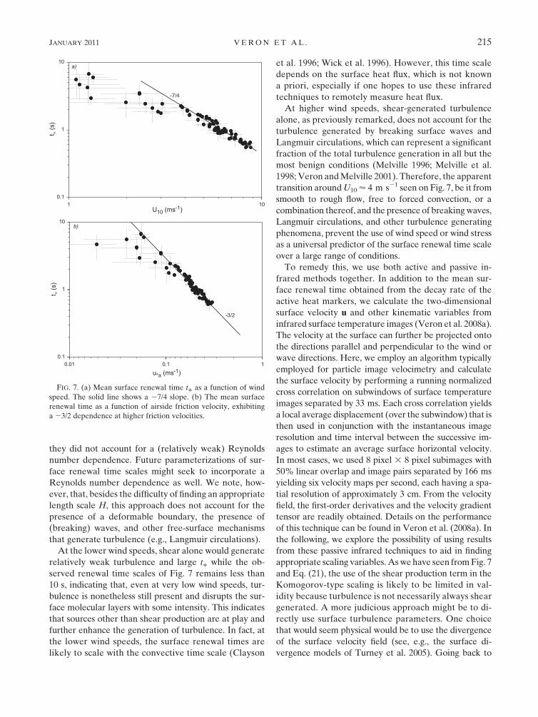
wind forcing. Indeed, Fig. 7 shows the mean renewal time

t*

as a function of wind speed and airside friction veloc-

ity and a decrease with increasing wind forcing. It also

shows that t*

; U�7/410 and t

*; u�3/2

*afor 4 m s21 , U10 ,

10 m s21, indicating that u*a ; U7/610 in this regime.

This also indicates, at least for this regime, that the drag

coefficient is a weak function of the wind speed CD ; U1/310 ,

which is in agreement with accepted parameterizations of

the drag coefficient (Fairall et al. 1996, 2003).

At wind speeds where U10 , 4 m s21, the surface re-

newal time scale departs from these trends and remains

FIG. 4. Pairs of SST images taken 0.665 s apart. The images show the Lagrangian heat markers (lighter spots) and are taken for wind

speeds of (a),(b) 0.5 m s21; (c),(d) 3 m s21; and (e),(f) 6.5 m s21. The arrow shows the wind direction. Note how the active TMV pattern

fades with time and is displaced, rotated, dilated, and sheared by the surface velocity field. Note also the development of linear tem-

perature structures at the higher wind speeds.


relatively low, albeit with some scatter in the data. This

likely indicates that, as suggested by Soloviev and

Schlussel (1994) and Wick (1995), the low wind speed

regime might be dominated by free convection. We note

that this transition in the data also corresponds to the

transition from smooth to rough flow (Kraus and Businger

1994); however, there is no reason to anticipate that the

turbulence would remain relatively high (i.e., the renewal

time scale would remain low) in the smooth flow limit.

These results are also consistent with our previous

measurements of surface turbulence statistics showing

that, in the field, surface turbulence remains, even at

very low wind speeds (Veron et al. 2008a).

If shear turbulence were to account for the surface

renewal events for wind speeds U10 . 4 m s21, the sur-

face renewal time scale, as first suggested by Brutsaert

(1975), should be equivalent to the Kolmogorov time

scale; that is, tk 5 (nw /�)1/2 in which nw is the kinematic

viscosity of water and � is the turbulent kinetic energy

dissipation. This form of the surface renewal time scale,

which assumes that there is a balance between dissipation

and production of turbulence by the mean shear flow, was

adopted in the landmark paper by Liu, Katsaros, and

Businger (1979). Later, equivalent parameterizations

were developed by Soloviev and Schlussel (1994) and

Wick (1995) who, in addition, considered the effect of

free convection at low wind speeds. Here

tk

5u2

*w›U/›z

nw

!�1/2

;u2

*wU

0

nw

H

!�1/2

, (21)

where U0 and u*w

are the surface drift velocity and the

waterside friction velocity, respectively, and where the

shear is estimated with outer scales with H a length scale

therefore associated with the shear boundary layer. If we

choose to parameterize surface renewal in this man-

ner and assume that our measured t*

; tk, and since

rau2*a

5 rwu2*w

, we find that H1/2;U1/20 u�1/2

*w; U1/2

0 u�1/2*a

.

Considering that the surface drift is a fraction of the at-

mospheric 10-m wind speed U0 ; O(1022)U10, we find

that H ; C�1/2D ; U�1/6

10 and H is nearly constant for

U10 . 4 m s21. This indicates that the length scale asso-

ciated with the waterside shear layer subjected to surface

renewal events becomes smaller with increasing wind

speed, albeit quite weakly. If we then define a Reynolds

number based on these outer scales (i.e., U0 and H),

Re 5U

0H

nw

, (22)

we find that the scaling of the renewal time scale with

inner variables (i.e., u*w) depends weakly on the Reynolds

number:

t*

u2*w

nw

; Re7/10. (23)

This is consistent with the results of Kim et al. (1971) and

Luchik and Tiederman (1987), who found dependences

of Re0.76 and Re0.73, respectively, for the time scales as-

sociated with turbulent bursts ejected from a solid

boundary. We also note that tr

; nw

/u2*w

is the surface

renewal time scale used by Soloviev and Schlussel

(1994) for moderate wind speeds. In a sense, this ap-

proach differs from their parameterization only in that

FIG. 5. Measured skin 2 subskin temperature difference as a

function of wind speed. For reference, we also show (gray triangles)

estimates of the skin 2 subskin temperature difference using Sa-

unders formula (Saunders 1967) with l 5 2.4 (Ward and Donelan

2006).

FIG. 6. Normalized surface temperature evolution of the active

heat markers laid down on the surface by the CO2 laser for dif-

ferent wind speeds ranging from 0.5 to 8.8 m s21. The inset shows

a single curve (diamonds) obtained from averaging all available

individual spot temperatures Tn (0, t) for 1 min at U10 5 5.4 m s21.

The gray curve is the theoretical prediction from Eq. (5).


they did not account for a (relatively weak) Reynolds

number dependence. Future parameterizations of sur-

face renewal time scales might seek to incorporate a

Reynolds number dependence as well. We note, how-

ever, that, besides the difficulty of finding an appropriate

length scale H, this approach does not account for the

presence of a deformable boundary, the presence of

(breaking) waves, and other free-surface mechanisms

that generate turbulence (e.g., Langmuir circulations).

At the lower wind speeds, shear alone would generate

relatively weak turbulence and large t*

while the ob-

served renewal time scales of Fig. 7 remains less than

10 s, indicating that, even at very low wind speeds, tur-

bulence is nonetheless still present and disrupts the sur-

face molecular layers with some intensity. This indicates

that sources other than shear production are at play and

further enhance the generation of turbulence. In fact, at

the lower wind speeds, the surface renewal times are

likely to scale with the convective time scale (Clayson

et al. 1996; Wick et al. 1996). However, this time scale

depends on the surface heat flux, which is not known

a priori, especially if one hopes to use these infrared

techniques to remotely measure heat flux.

At higher wind speeds, shear-generated turbulence

alone, as previously remarked, does not account for the

turbulence generated by breaking surface waves and

Langmuir circulations, which can represent a significant

fraction of the total turbulence generation in all but the

most benign conditions (Melville 1996; Melville et al.

1998; Veron and Melville 2001). Therefore, the apparent

transition around U10 ’ 4 m s21 seen on Fig. 7, be it from

smooth to rough flow, free to forced convection, or a

combination thereof, and the presence of breaking waves,

Langmuir circulations, and other turbulence generating

phenomena, prevent the use of wind speed or wind stress

as a universal predictor of the surface renewal time scale

over a large range of conditions.

To remedy this, we use both active and passive in-

frared methods together. In addition to the mean sur-

face renewal time obtained from the decay rate of the

active heat markers, we calculate the two-dimensional

surface velocity u and other kinematic variables from

infrared surface temperature images (Veron et al. 2008a).

The velocity at the surface can further be projected onto

the directions parallel and perpendicular to the wind or

wave directions. Here, we employ an algorithm typically

employed for particle image velocimetry and calculate

the surface velocity by performing a running normalized

cross correlation on subwindows of surface temperature

images separated by 33 ms. Each cross correlation yields

a local average displacement (over the subwindow) that is

then used in conjunction with the instantaneous image

resolution and time interval between the successive im-

ages to estimate an average surface horizontal velocity.

In most cases, we used 8 pixel 3 8 pixel subimages with

50% linear overlap and image pairs separated by 166 ms

yielding six velocity maps per second, each having a spa-

tial resolution of approximately 3 cm. From the velocity

field, the first-order derivatives and the velocity gradient

tensor are readily obtained. Details on the performance

of this technique can be found in Veron et al. (2008a). In

the following, we explore the possibility of using results

from these passive infrared techniques to aid in finding

appropriate scaling variables. As we have seen from Fig. 7

and Eq. (21), the use of the shear production term in the

Komogorov-type scaling is likely to be limited in val-

idity because turbulence is not necessarily always shear

generated. A more judicious approach might be to di-

rectly use surface turbulence parameters. One choice

that would seem physical would be to use the divergence

of the surface velocity field (see, e.g., the surface di-

vergence models of Turney et al. 2005). Going back to

FIG. 7. (a) Mean surface renewal time t*

as a function of wind

speed. The solid line shows a 27/4 slope. (b) The mean surface

renewal time as a function of airside friction velocity, exhibiting

a 23/2 dependence at higher friction velocities.


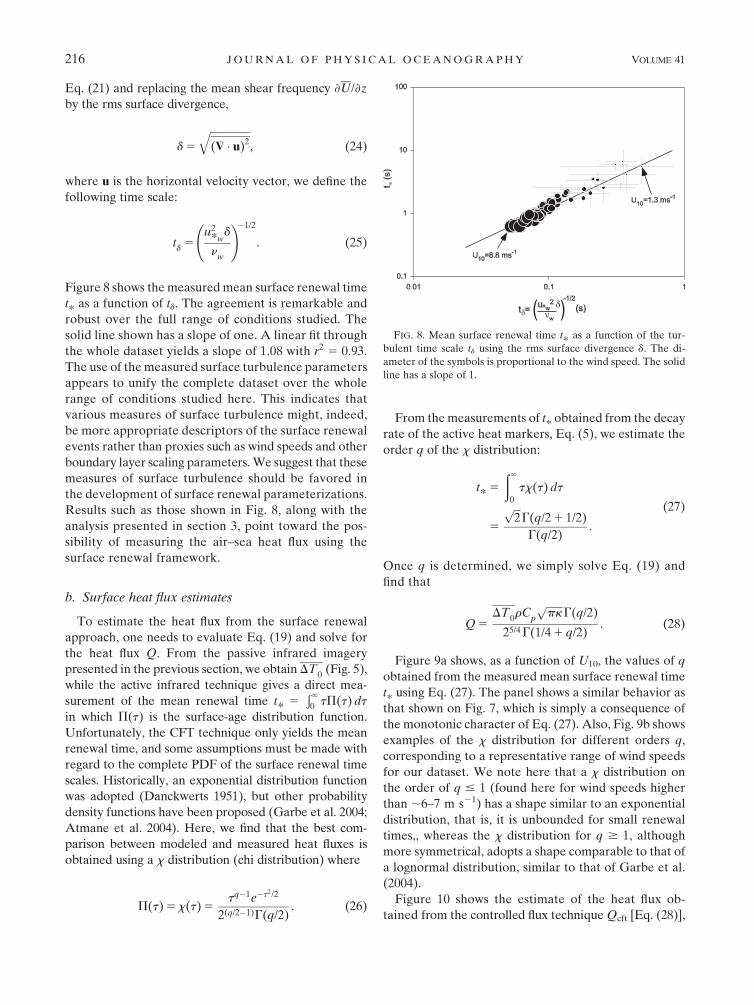
Eq. (21) and replacing the mean shear frequency ›U/›z

by the rms surface divergence,

d 5

ffiffiffiffiffiffiffiffiffiffiffiffiffiffiffi($ � u)2

q, (24)

where u is the horizontal velocity vector, we define the

following time scale:

td

5u2

*wd

nw

!�1/2

. (25)

Figure 8 shows the measured mean surface renewal time

t*

as a function of td. The agreement is remarkable and

robust over the full range of conditions studied. The

solid line shown has a slope of one. A linear fit through

the whole dataset yields a slope of 1.08 with r2 5 0.93.

The use of the measured surface turbulence parameters

appears to unify the complete dataset over the whole

range of conditions studied here. This indicates that

various measures of surface turbulence might, indeed,

be more appropriate descriptors of the surface renewal

events rather than proxies such as wind speeds and other

boundary layer scaling parameters. We suggest that these

measures of surface turbulence should be favored in

the development of surface renewal parameterizations.

Results such as those shown in Fig. 8, along with the

analysis presented in section 3, point toward the pos-

sibility of measuring the air–sea heat flux using the

surface renewal framework.

b. Surface heat flux estimates

To estimate the heat flux from the surface renewal

approach, one needs to evaluate Eq. (19) and solve for

the heat flux Q. From the passive infrared imagery

presented in the previous section, we obtain DT0

(Fig. 5),

while the active infrared technique gives a direct mea-

surement of the mean renewal time t*

5Ð ‘

0 tP(t) dt

in which P(t) is the surface-age distribution function.

Unfortunately, the CFT technique only yields the mean

renewal time, and some assumptions must be made with

regard to the complete PDF of the surface renewal time

scales. Historically, an exponential distribution function

was adopted (Danckwerts 1951), but other probability

density functions have been proposed (Garbe et al. 2004;

Atmane et al. 2004). Here, we find that the best com-

parison between modeled and measured heat fluxes is

obtained using a x distribution (chi distribution) where

P(t) 5 x(t) 5tq�1e�t2/2

2(q/2�1)G(q/2). (26)

From the measurements of t*

obtained from the decay

rate of the active heat markers, Eq. (5), we estimate the

order q of the x distribution:

t*

5

ð‘

0

tx(t) dt

5

ffiffiffi2p

G(q/2 1 1/2)

G(q/2).

(27)

Once q is determined, we simply solve Eq. (19) and

find that

Q 5DT

0rC

p

ffiffiffiffiffiffipkp

G(q/2)

25/4 G(1/4 1 q/2). (28)

Figure 9a shows, as a function of U10, the values of q

obtained from the measured mean surface renewal time

t*

using Eq. (27). The panel shows a similar behavior as

that shown on Fig. 7, which is simply a consequence of

the monotonic character of Eq. (27). Also, Fig. 9b shows

examples of the x distribution for different orders q,

corresponding to a representative range of wind speeds

for our dataset. We note here that a x distribution on

the order of q # 1 (found here for wind speeds higher

than ;6–7 m s21) has a shape similar to an exponential

distribution, that is, it is unbounded for small renewal

times,, whereas the x distribution for q $ 1, although

more symmetrical, adopts a shape comparable to that of

a lognormal distribution, similar to that of Garbe et al.

(2004).

Figure 10 shows the estimate of the heat flux ob-

tained from the controlled flux technique Qcft [Eq. (28)],

FIG. 8. Mean surface renewal time t*

as a function of the tur-

bulent time scale td using the rms surface divergence d. The di-

ameter of the symbols is proportional to the wind speed. The solid

line has a slope of 1.


compared with the net heat flux Qnet measured with the

meteorological package. The solid line shows the one-

to-one correspondence. The agreement is acceptable

and the estimate of the net heat flux from the CFT is

within a factor of 2 of the net heat flux measured di-

rectly. This is in contrast to the measurements of Asher

et al. (2004), who found that their CFT measurements

overestimated the heat flux by up to a factor of 7. Al-

though the agreement found here is satisfactory, espe-

cially at the higher heat fluxes, it appears that the low

heat flux regime (less than about 100 W m22) exhibits

larger errors. Other surface-age distribution functions

might lead to similar results. For instance, we find that

surface-age distributions with surface renewal times

distributed like powers of a x distribution between x and

x2, such as x3/2, or a Maxwell–Boltzmann distribution

lead to similarly acceptable results overall, with improved

agreement in the low heat flux regime. However, over the

full dataset, the mean error is not significantly improved,

and it is not possible to unequivocally determine a single

surface-age distribution function that is universally

satisfactory. It is conceivable, and perhaps likely, that

not one distribution can be used to represent a wide

range of forcing conditions and turbulent regimes.

Furthermore, it has also been suggested that, rather

than having a temporal distribution of surface renewal

events, these might instead be distributed in space with

turbulent eddies possibly renewing the surface layer

only partially (Atmane et al. 2004; Jessup et al. 2009).

Regardless of the surface-age PDF, a crucial param-

eter, which in fact appears to be the main source of

the difference between the results presented here and

that of Asher et al. (2004), is the value of DT0 used in

Eq. (19).

5. Conclusions

We have shown that the surface renewal theory orig-

inally presented by Higbie (1935) and later applied by

Danckwerts (1951) for gas transfer applications was

perhaps hastily applied to the heat transfer problem.

Indeed, while the basic physics of these scalar transfers

through the molecular diffusive surface layers are iden-

tical, we showed that the difference in surface boundary

conditions for heat and gas, namely constant flux and

constant concentration difference, respectively, lead to

vastly different solutions to the simple diffusion prob-

lem. However, within the surface renewal framework,

the relationship between skin 2 subskin temperature

difference and surface heat flux (i.e., the Fickian dif-

fusion law) is identical for both surface conditions if

the PDF of the surface renewal times is strictly given by

FIG. 9. (a) Estimate of the order q of the x distribution as a

function of wind speed. (b) Several examples of the functional

shape of the x distribution for multiple q corresponding to a wide

range of wind speeds.

FIG. 10. Estimate of the heat flux obtained from the controlled

flux technique, Qcft from Eq. (28), compared with the net heat flux

Qnet measured with the eddy covariance system. The diameter of

the symbols is proportional to the wind speed and the solid line

shows the one-to-one correspondence.


an exponential distribution. This PDF is widely used in

the, so-called, controlled-flux technique that uses active

surface thermal markers to directly estimate the mean

surface renewal rates. Therefore, previous estimates of

heat fluxes made with the CFT technique are not in

error provided that the PDF of surface renewal times is,

indeed, exponential. We note here that the active CFT

technique gives an estimate of the mean surface renewal

rate, which is the first moment of the exponential distri-

bution, but does not measure the PDF itself. In fact,

recent work (Garbe et al. 2004; Atmane et al. 2004),

including the results presented in this paper, suggests

that other PDFs might also be appropriate. The x dis-

tribution leads to an accurate description of the skin 2

subskin temperature difference, and we show that it

leads to a reasonable estimate of the surface heat flux.

If surface renewal time scales are better described by

PDFs other than exponential, then the different solu-

tions to the diffusion problem for heat and gas (for

different boundary conditions) cast doubts on the use

of heat as a proxy for surface gas transfer estimates.

This is separate from the fact that air–sea surface heat

transfer can never account for the contribution of bub-

ble entrainment to gas transfer. Finally, we showed that,

at moderate wind speeds, the surface renewal time scale

compares favorably with the rate of ejection of a turbu-

lent burst from turbulent boundary layers over flat solid

surfaces, provided that the outer scaling involves a nearly

constant boundary layer depth. At low wind speeds, it is

likely that turbulent convection dominates, whereas over

the intermediate wind speeds the shear generation of tur-

bulence might be more significantly affected by breaking

surface waves and Langmuir circulations. Finally, we have

shown that the surface renewal rate scales very well with

surface turbulent parameters over the whole range of slow

and intermediate wind speeds studied here. In particular,

when using the rms surface divergence, we derived a time

scale that predicts the measured surface renewal time scale

robustly and independently of the turbulence generation

mechanisms. We conclude that the direct use of surface

turbulence measurements will be a more productive ap-

proach for studying and better understanding air–sea sca-

lar fluxes.

Acknowledgments. We thank Peter Matusov for his

help in the design, construction, testing, and deployment

of the original instrumentation. We thank Bill Gaines

and the captain and crew of the R/P FLIP for all their

help in the field experiments. We thank John Hildebrand

and Gerald D’Spain for sharing space and facilities on

FLIP. This research was supported by an NSF grant

(OCE 01-18449) to WKM and FV and an ONR (Physical

Oceanography) grant to WKM.

REFERENCES

Agrawal, Y., E. Terray, M. A. Donelan, P. Hwang, A. J. Williams

III, W. M. Drennan, K. K. Kahma, and S. A. Kitaigorodskii,

1992: Enhanced dissipation of kinetic energy beneath surface

waves. Nature, 359, 219–220.

Andreas, E. L, 2004: Spray stress revisited. J. Phys. Oceanogr., 34,

1429–1440.

Anis, A., and J. N. Moum, 1995: Surface wave–turbulence in-

teractions: Scaling �(z) near the sea surface. J. Phys. Ocean-

ogr., 25, 2025–2045.

Asher, W. E., and J. F. Pankow, 1989: Direct observations of

concentration fluctuations close to a gas-liquid interface.

Chem. Eng. Sci., 44, 1451–1455.

——, A. T. Jessup, and M. A. Atmane, 2004: Oceanic application of

the active controlled flux technique for measuring air-sea

transfer velocities of heat and gases. J. Geophys. Res., 109,

C08S12, doi:10.1029/2003JC001862.

Atmane, M. A., W. E. Asher, and A. T. Jessup, 2004: On the use of

the active infrared technique to infer heat and gas transfer

velocities at the air-water free surface. J. Geophys. Res., 109,

C08S14, doi:10.1029/2003JC001805.

Brutsaert, W., 1975: A theory for local evaporation (or heat

transfer) from rough and smooth surfaces at ground level.

Water Resour. Res., 11, 543–550.

Businger, J. A., J. C. Wyngaard, Y. Izumi, and E. F. Bradley, 1971:

Flux-profile relationships in the atmospheric surface layer.

J. Atmos. Sci., 28, 181–189.

Castro, S. L., G. A. Wick, and W. J. Emery, 2003: Further re-

finements to models for the bulk-skin sea surface tempera-

ture difference. J. Geophys. Res., 108, 3377, doi:10.1029/

2002JC001641.

Clayson, C. A., C. W. Fairall, and J. A. Curry, 1996: Evaluation of

turbulent fluxes at the ocean surface using surface renewal

theory. J. Geophys. Res., 101, 28 503–28 513.

Danckwerts, P. V., 1951: Significance of liquid-film coefficients in

gas absorption. Ind. Eng. Chem., 43, 1460–1467.

Donelan, M. A., B. K. Haus, N. Reul, W. J. Plant, M. Stiassnie,

H. C. Graber, O. B. Brown, and E. S. Saltzman, 2004: On

the limiting aerodynamics roughness on the ocean in very

strong winds. Geophys. Res. Lett., 31, L18306, doi:10.1029/

2004GL019460.

Donlon, C. J., and I. S. Robinson, 1997: Observations of the oceanic

thermal skin in the Atlantic Ocean. J. Geophys. Res., 102,

18 585–18 606.

——, W. Eifler, and T. J. Nightindale, 1999: The thermal skin

temperature of the ocean at high wind speed. Proc. Int. Geo-

science and Remote Sensing Symposium (IGARSS), Hamburg,

Germany, IEEE, Vol. 1, 8–10.

——, P. J. Minnett, C. Gentemann, T. J. Nightingale, I. J. Barton,

B. Ward, and M. J. Murray, 2002: Toward improved validation

of satellite sea surface skin temperature measurements for

climate research. J. Climate, 15, 353–369.

Downing, H. D., and D. Williams, 1975: Optical constant of water

in the infrared. J. Geophys. Res., 80, 1656–1661.

Drennan, W. M., M. A. Donelan, E. A. Terray, and K. B. Katsaros,

1996: Oceanic turbulence dissipation measurements in SWADE.

J. Phys. Oceanogr., 26, 808–815.

Edson, J. B., C. J. Zappa, J. A. Ware, W. R. McGillis, and

J. E. Hare, 2004: Scalar flux profile relationships over the open

ocean. J. Geophys. Res., 109, C08S09, doi:10.1029/2003JC001960.

Ewing, G., and E. D. McAlister, 1960: On the thermal boundary

layer of the ocean. Science, 131, 1374–1376.


Fairall, C. W., E. F. Bradley, D. P. Rogers, J. B. Edson, and

G. S. Young, 1996: Bulk parameterization of air-sea fluxes for

Tropical Ocean-Global Atmosphere Coupled-Ocean Atmo-

sphere Response Experiment. J. Geophys. Res., 101, 3747–

3764.

——, ——, J. E. Hare, A. A. Grachev, and J. B. Edson, 2003: Bulk

parameterization of air–sea fluxes: Updates and verification

for the COARE algorithm. J. Climate, 16, 571–591.

Farmer, D. M., C. L. McNeil, and B. D. Johnson, 1993: Evidence

for the importance of bubbles in increasing air–sea gas flux.

Nature, 361, 620–623.

Frew, N. M., and Coauthors, 2004: Air-sea gas transfer: Its de-

pendence on wind stress, small-scale roughness, and surface

films. J. Geophys. Res., 109, C08S17, doi:10.1029/2003JC002131.

Garbe, C. S., U. Schimpf, and B. Jahne, 2004: A surface renewal

model to analyze infrared image sequences of the ocean sur-

face for the study of air-sea heat and gas exchange. J. Geophys.

Res., 109, C08S15, doi:10.1029/2003JC001802.

Gemmrich, J., and D. Farmer, 2004: Near-surface turbulence

in the presence of breaking waves. J. Phys. Oceanogr., 34,

1067–1086.

Hara, T., and S. E. Belcher, 2002: Wind forcing in the equilibrium

range of wind-wave spectra. J. Fluid Mech., 470, 223–245.

Haußecker, H., 1996: Messung und simulation von kleinskaligen

austauschvorgangen an de ozeanoberflache mittels ther-

mographie. Ph.D. dissertation, University of Heidelberg,

197 pp.

——, S. Reinelt, and B. Jahne, 1995: Heat as a proxy tracer for gas

exchange measurements in the field: Principles and technical

realization. Air–Water Gas Transfer, B. Jahne and E. C.

Monahan, Eds., Aeon-Verlag, 405–413.

——, U. Schimpf, C. S. Garbe, and B. Jahne, 2001: Physics from IR

image sequences: Quantitative analysis of transport models

and parameters of air-sea gas transfer. Gas Transfer at Water

Surfaces, Geophys. Monogr., Vol. 127, Amer. Geophys. Un-

ion, 103–108.

Higbie, R., 1935: The rate of absorption of a pure gas into a still

liquid during short periods of exposure. Trans. Amer. Inst.

Chem. Eng., 31, 365–389.

Ho, D. T., F. Veron, E. Harrison, L. F. Bliven, N. Scott, and

W. R. McGillis, 2007: The combined effect of rain and wind on

air–water gas exchange: A feasibility study. J. Mar. Syst., 66

(1–4), 150–160.

Hsu, C.-T., E. Y. Hsu, and R. L. Street, 1981: On the structure of

turbulent flow over a progressive water wave: Theory and

experiment in a transformed, wave-following co-ordinate

system. J. Fluid Mech., 105, 87–117.

Jahne, B., and H. Haußecker, 1998: Air-water gas exchange. Annu.

Rev. Fluid Mech., 30, 443–468.

——, P. Libner, R. Fisher, T. Billen, and E. J. Plate, 1989: In-

vestigating the transfer processes across the free aqueous

viscous boundary layer by the controlled flux method. Tellus,

41, 177–195.

Jessup, A. T., C. J. Zappa, M. R. Loewen, and V. Hesany, 1997a:

Infrared remote sensing of breaking waves. Nature, 385,

52–55.

——, ——, and J. H. Yeh, 1997b: Defining and quantifying mi-

croscale breaking with infrared imagery. J. Geophys. Res., 102,

23 145–23 153.

——, W. E. Asher, M. Atmane, K. Phadnis, C. J. Zappa, and

M. R. Loewen, 2009: Evidence for complete and partial sur-

face renewal at an air-water interface. Geophys. Res. Lett., 36,

L16601, doi:10.1029/2009GL038986.

Katsaros, K. B., 1980: The aqueous thermal boundary layer. Bound.-

Layer Meteor., 18, 107–127.

Kim, H. T., S. J. Kline, and W. C. Reynolds, 1971: The production

of turbulence near smooth wall in a turbulent boundary layer.

J. Fluid Mech., 50, 133–160.

Kitaigorodskii, S. A., 1984: On the fluid dynamical theory of tur-

bulent gas transfer across an air–sea interface in the presence

of breaking wind-waves. J. Phys. Oceanogr., 14, 960–972.

Komen, G. J., L. Cavaleri, M. Donelan, K. Hasselmann, S. Hasselmann,

and P. A. E. M. Janssen, 1994: Dynamics and Modelling of Ocean

Waves. Cambridge University Press, 532 pp.

Kraus, E. B., and J. A. Businger, 1994: Atmosphere-Ocean In-

teraction. Oxford University Press, 362 pp.

Kudryavtsev, V. N., and V. K. Makin, 2001: The impact of air-flow

separation on the drag of the sea surface. Bound.-Layer Me-

teor., 98, 155–171.

Liu, W. T., K. B. Katsaros, and J. A. Businger, 1979: Bulk param-

eterization of the air–sea exchange of heat and water vapor

including the molecular constraints at the interface. J. Atmos.

Sci., 36, 1722–1735.

Luchik, T., and W. G. Tiederman, 1987: Timescale and structure of

ejections and bursts in turbulent channel flows. J. Fluid Mech.,

174, 529–552.

McAlister, E. D., 1964: Infrared optical techniques applied to

oceanography I. Measurement of total heat flow form the sea

surface. Appl. Opt., 5, 609–612.

——, and W. McLeish, 1970: A radiometric system for airborne

measurement of the total heat flow from the sea. Appl. Opt., 9,

2607–2705.

Melville, W. K., 1994: Energy dissipation by breaking waves.

J. Phys. Oceanogr., 24, 2041–2049.

——, 1996: The role of surface-wave breaking in air-sea in-

teraction. Annu. Rev. Fluid Mech., 28, 279–321.

——, R. Shear, and F. Veron, 1998: Laboratory measurements

of the generation and evolution of Langmuir circulations.

J. Fluid Mech., 364, 31–58.

——, F. Veron, and C. J. White, 2002: The velocity field under

breaking waves: Coherent structures and turbulence. J. Fluid

Mech., 454, 203–233.

Mueller, J. A., and F. Veron, 2009a: Nonlinear formulation of the

bulk surface stress over breaking waves: Feedback mecha-

nisms from air-flow separation. Bound.-Layer Meteor., 130,

117–134.

——, and ——, 2009b: A sea state–dependent spume generation

function. J. Phys. Oceanogr., 39, 2363–2372.

Panofsky, H. A., and J. A. Dutton, 1984: Atmospheric Turbulence:

Models and Methods for Engineering Applications. John

Wiley, 397 pp.

Paulson, C. A., and J. J. Simpson, 1981: The temperature difference

across the cool skin of the ocean. J. Geophys. Res., 86 (C11),

11 044–11 054.

Rapp, R. J., and W. K. Melville, 1990: Laboratory measurements of

deep-water breaking waves. Philos. Trans. Roy. Soc. London,

331A, 735–800.

Saunders, P. M., 1967: The temperature of the ocean-air interface.

J. Atmos. Sci., 24, 269–273.

Schimpf, U., C. Garbe, and B. Jahne, 2004: Investigation of transport

processes across the sea surface microlayer by infrared imagery.

J. Geophys. Res., 109, C08S13, doi:10.1029/2003JC001803.

Schlussel, P., W. J. Emery, H. Grassl, and T. Mammen, 1990: On

the bulk-skin temperature difference and its impact on satel-

lite remote sensing of the sea surface temperature. J. Geophys.

Res., 95, 13 341–13 356.


Snyder, R. L., F. W. Dobson, J. A. Elliott, and R. B. Long, 1981:

Array measurements of atmospheric pressure fluctuations

above surface gravity waves. J. Fluid Mech., 102, 1–59.

Soloviev, A. V., and P. Schlussel, 1994: Parameterization of the

cool skin of the ocean and the air–ocean gas transfer on the

basis of modeling surface renewal. J. Phys. Oceanogr., 24,

1339–1346.

Sullivan, P. P., and J. C. McWilliams, 2002: Turbulent flow over

water waves in the presence of stratification. Phys. Fluids, 14,

1182–1195.

——, ——, and C.-H. Moeng, 2000: Simulation of turbulent flow

over idealized water waves. J. Fluid Mech., 404, 47–85.

——, ——, and W. K. Melville, 2004: The oceanic boundary

layer driven by wave breaking with stochastic variability.

Part I: Direct numerical simulations. J. Fluid Mech., 507,143–174.

——, ——, and ——, 2007: Surface gravity wave effects in

the oceanic boundary layer: Large-eddy simulation with

vortex force and stochastic breakers. J. Fluid Mech., 593,405–452.

Teixeira, M. A. C., and S. E. Belcher, 2002: On the distortion of

turbulence by a progressive surface wave. J. Fluid Mech., 458,

229–267.

Terray, E., M. A. Donelan, Y. Agrawal, W. M. Drennan, K. K.

Kahma, A. J. Williams III, P. Hwang, and S. A. Kitaigorodskii,

1996: Estimates of kinetic energy dissipation under breaking

waves. J. Phys. Oceanogr., 26, 792–807.

Thorpe, S. A., 1993: Energy loss by breaking waves. J. Phys. Oce-

anogr., 23, 2498–2502.

——, T. R. Osborn, D. M. Farmer, and S. Vagle, 2003: Bubble

clouds and Langmuir circulation: Observations and models.

J. Phys. Oceanogr., 33, 2013–2031.

Turney, D. E., W. C. Smith, and S. Banerjee, 2005: A measure

of near-surface fluid motions that predicts air-water gas in

a wide range of conditions. Geophys. Res. Lett., 32, L04607,

doi:10.1029/2004GL021671.

Veron, F., and W. K. Melville, 1999: Pulse-to-pulse coherent

Doppler measurements of waves and turbulence. J. Atmos.

Oceanic Technol., 16, 1580–1597.

——, and ——, 2001: Experiments on the stability and transition of

wind-driven water surfaces. J. Fluid Mech., 446, 25–65.

——, G. Saxena, and S. K. Misra, 2007: Measurements of the vis-

cous tangential stress in the airflow above wind waves. Geo-

phys. Res. Lett., 34, L19603, doi:10.1029/2007GL031242.

——, W. K. Melville, and L. Lenain, 2008a: Infrared techniques for

measuring ocean surface processes. J. Atmos. Oceanic Tech-

nol., 25, 307–326.

——, ——, and ——, 2008b: Wave-coherent air–sea heat flux.


——, ——, and ——, 2009: Measurements of ocean surface tur-

bulence and wave–turbulence interactions. J. Phys. Oceanogr.,

39, 2310–2323.

Ward, B., 2006: Near-surface ocean temperature. J. Geophys. Res.,

111, C02004, doi:10.1029/2004JC002689.

——, and M. A. Donelan, 2006: Thermometric measurements of

the molecular sublayer at the air-water interface. Geophys.

Res. Lett., 33, L07605, doi:10.1029/2005GL024769.

Webb, E. K., G. I. Pearman, and R. Leuning, 1980: Measurements

for density effects due to heat and water vapor transfer. Quart.

J. Roy. Meteor. Soc., 106, 85–106.

Wick, G. A., 1995: Evaluation of the variability and predictability

of the bulk-skin SST difference with application to satellite-

measured SST. Ph.D. dissertation, University of Colorado,

146 pp.

——, W. J. Emery, and P. Schlussel, 1992: A comprehensive

comparison between satellite-measured skin and multichan-

nel sea surface temperature. J. Geophys. Res., 97 (C4), 5569–

5595.

——, ——, L. H. Kantha, and P. Schlussel, 1996: The behavior

of the bulk 2 skin sea surface temperature difference under

varying wind speed and heat flux. J. Phys. Oceanogr., 26,

1969–1988.

——, J. C. Ohlmann, C. W. Fairall, and A. T. Jessup, 2005: Im-

proved oceanic cool-skin corrections using a refined solar

penetration model. J. Phys. Oceanogr., 35, 1986–1996.

Zappa, C. J., W. E. Asher, and A. T. Jessup, 2001: Microscale wave

breaking and air-water gas transfer. J. Geophys. Res., 106 (C5),

9385–9391.


CORRIGENDUM

FABRICE VERON

School of Marine Science and Policy, University of Delaware, Newark, Delaware

W. KENDALL MELVILLE AND LUC LENAIN

Scripps Institution of Oceanography, University of California, San Diego, La Jolla, California

Because of a production error in Veron et al. (2011), Eq. (9) was incorrect. The correct

equation is as follows:

Q(t) 5 �i

aiti. (9)

AMS and the staff of the Journal of Physical Oceanography regret any inconvenience this

error may have caused.

REFERENCE

Veron, F., W. K. Melville, and L. Lenain, 2011: The effects of small-scale turbulence on air–sea heat flux.


Corresponding author address: Fabrice Veron, 112C Robinson Hall. University of Delaware, School of Marine Science and Policy,

College of Earth, Ocean and Environment, Newark, DE 19716.

E-mail: [email protected]

AUGUST 2011 C O R R I G E N D U M 1583

DOI: 10.1175/JPO-D-11-091.1

� 2011 American Meteorological Society

the effects of small-scale turbulence on air–sea...

Documents