the effects of exhaust gas recirculation on combustion and
TRANSCRIPT

THE EFFECTS OF EXHAUST GAS
RECIRCULATION ON COMBUSTION AND EMISSIONS IN AN AIR-COOLED UTILITY
ENGINE
by
Nathan Jon Haugle
A thesis submitted in partial fulfillment of the requirements for the degree of
Master of Science (Mechanical Engineering)
at the
UNIVERSITY OF WISCONSIN-MADISON
2006

2
Approved:_____________________ Date:_____________ Associate Professor Jaal B. Ghandhi Department of Mechanical Engineering University of Wisconsin - Madison

i
ABSTRACT
Among other requirements, small air-cooled utility engines must maximize power-to-
weight ratio. A means of meeting this requirement is to optimize the gas exchange process
by utilizing cam shafts that complement high speed, wide open throttle (WOT) performance.
The resulting valve timing tends to cause high levels of exhaust gas retention, or residual, at
low-speed, light-load conditions, giving rise to poor combustion stability and idle quality.
The effects of residual gas level and homogeneity were studied in a single-cylinder,
air-cooled utility engine using both external exhaust gas recirculation (EGR) and internal
residual retention. EGR was introduced far upstream of the throttle to ensure proper mixing.
Internal residual was changed by varying the length of the valve overlap period.
The total in-cylinder diluent was measured directly using a skip-fire cylinder
dumping technique. A sweep of diluent fraction was performed for several engine speeds,
engine loads, fuel mixture preparation systems, and ignition timings. An optimum level of
diluent, where the combined hydrocarbon (HC) and oxides of nitrogen (NOx) emissions were
minimal, was found to exist for each operating condition. Higher levels of diluent, either
through internal retention or external recirculation, caused the combined emissions to
increase. The transition to higher emissions levels was found to correspond to conditions
where the heat release rate extends to the point of exhaust valve opening. Combustion with a
high level of variability, but heat release completing prior to exhaust valve opening, did not
adversely affect the hydrocarbon emissions. This was observed by direct analysis of
individual-cycle hydrocarbon emissions and combustion performance.

ii
Complementary studies investigated how fuel mixture preparation, residual mixedness,
intake volume, ignition timing, spark energy and volume affect combustion quality and
emissions.
Optimizing the spark timing improved the combustion quality in highly diluted
conditions by improving phasing, reducing cyclic variability, and decreasing the burn
duration. Similar behavior to stock ignition conditions with regards to hydrocarbon
emissions was found; however, improvements in diluent tolerance and combustion quality
did not result in reduced emissions.
Residual gas mixing, or the source of diluent, appeared to have little effect on the
trends seen in combustion or emissions. The trends were found to be only a function of
overall diluent fraction. Optimizing the ignition at high levels of diluent appeared to
improve combustion quality more easily in the EGR supplemented cases compared to the
maximum overlap cases.
Very slight improvements in cyclic variability, combustion phasing, and heat release
rate were noted with increased spark gap and, to a lesser degree, spark energy. Combustion
quality reduced significantly at very low energy and hydrocarbon emissions drastically
increased as a result.

iii
Dedicated to my Grandfathers; Thomas Hill and Juel Haugle

iv
ACKNOWLEDGEMENTS
There have been so many who have provided helping hands and encouragement
throughout this project. At the top of it all, Professor Jaal Ghandhi, whose guidance
throughout my work at the ERC has provided me with unforeseen opportunities, personal
direction, and broad knowledge. Thank you so much for your patients and kindness.
I would like to thank all the member companies of the Wisconsin Small Engine
Consortium: Briggs and Stratton, Harley-Davidson, Kohler, Mercury Marine, MotoTron,
Fleetguard Nelson Inc., and the Wisconsin Department of Commerce. In particular, I want to
thank Phil Pierce for his support throughout my undergraduate research fellowship, and for
his encouragement to follow though into graduate school. A special thanks to Blake Suhre
for help with engine control, and Art Poehlman, Eric Hudak, Tom Engman, Tony Coffey,
Chuck Eichinger, and Suzanne Caulfield for all of the help and input during the project.
Ralph Braun always came through with whatever task was required from the lab,
Andy Bright really took me under his wing early in my graduate career, Susie Strzelec
always helped answer questions both administrative and legal and everyone else at the ERC.
My family and upbringing have so much to do with why I became an engineer. From
my grandpa Tom’s tinkering and building, grandpa Juel’s unmatched mechanics touch, drag
racing with the cousins, Tim and Tom, before I could drive, helping my father with the
winter motorcycle maintenance, and my mother’s creative artwork and craftiness.
My parents and grandparents support and love have always made any of life’s paths
smooth. Thanks you so much. Last but not least, my girl who has been supportive during the
crunch time and has made the last two years great.

v
Table of Content ABSTRACT............................................................................................................................... i ACKNOWLEDGEMENTS..................................................................................................... iv Table of Content ....................................................................................................................... v LIST OF FIGURES ............................................................................................................... viii LIST OF TABLES................................................................................................................... xi NOMENCLATURE ............................................................................................................... xii 1.0 INTRODUCTION .............................................................................................................. 1
1.1 Motivation....................................................................................................................... 1 1.1.2 Small Engines .......................................................................................................... 2 1.1.2 Small Engine Emission Standards ........................................................................... 3
1.2 Objective ......................................................................................................................... 5 2.0 BACKGROUND AND LITERATURE REVIEW ............................................................ 7
2.1 Introduction..................................................................................................................... 7 2.2 Small Engine Emissions Testing .................................................................................... 8 2.3 Exhaust Gas Residual ..................................................................................................... 8
2.3.1 Exhaust Diluent Effects on Combustion and Emissions.......................................... 9 2.3.2 Internal Residual Gas............................................................................................. 11
2.3.2.1 Source of Internal Residual............................................................................. 11 2.3.2.2 Techniques for Residual Measurement........................................................... 12 2.3.2.3 Residual Prediction Techniques...................................................................... 12
2.3.3 Unique Conditions in the Small Engine................................................................. 15 2.3.3.1 Long Valve Overlap for Maximum Charging Efficiency............................... 15 2.3.3.2 Lack of Constant Intake Manifold Vacuum.................................................... 16 2.3.3.3 Small Engine Design Requirements ............................................................... 16
2.3.4 Residual Mixing..................................................................................................... 18 2.3.4.1 Mixing Behavior ............................................................................................. 18 2.3.4.2 Homogeneous Mixture Effects on Combustion.............................................. 18 2.3.4.3 Dilution Tolerance .......................................................................................... 19
2.4 Cyclic Variability.......................................................................................................... 20 2.4.1 Definition ............................................................................................................... 20 2.4.2 Characterizing of Cycle Variability ....................................................................... 21 2.4.3 Cycle-Resolved Hydrocarbon Measurements........................................................ 22
2.5 Fuel Mixture Preparation Effects on Combustion and Emissions ................................ 24 2.5.1 Carburetion ............................................................................................................ 26 2.5.2 Homogeneous Mixture........................................................................................... 26
2.6 Ignition Effects on Combustion .................................................................................... 27 2.6.1 Spark Timing ......................................................................................................... 27 2.6.2 Spark Energy.......................................................................................................... 28 2.6.3 Spark Volume ........................................................................................................ 28
3.0 EXPERIEMENTAL SETUP ............................................................................................ 30 3.1 Engine Description........................................................................................................ 30 3.2 Engine Dynamometer, Torque Sensor, and Shaft Encoder .......................................... 31

vi
3.3 Engine Control System ................................................................................................. 32 3.4 Fresh Air Delivery System............................................................................................ 33 3.5 Fuel System................................................................................................................... 35
3.5.1 Carburetor .............................................................................................................. 37 3.5.3 Homogeneous Mixture System.............................................................................. 37
3.6 Exhaust System............................................................................................................. 38 3.7 External Exhaust Gas Recirculation System................................................................. 39 3.8 Air-Fuel Ratio Analyzer ............................................................................................... 41 3.9 Ignition System ............................................................................................................. 42 3.10 Pressure Transducers .................................................................................................. 44 3.11 Data Acquisition Systems and Data Processing ......................................................... 44 3.12 Intake Sample System and In-Cylinder Sample Conditioning ................................... 46 3.13 Exhaust Emissions Analyzer....................................................................................... 47 3.14 Fast Flame Ionizing Detector...................................................................................... 48 3.15 In-cylinder Sampling Valve........................................................................................ 49
4.0 DILUENT MEASUREMENT AND ANALYSIS ........................................................... 52 4.1 Introduction................................................................................................................... 52 4.2 Experimental Operating Conditions ............................................................................. 52
4.2.1 EGR Study ............................................................................................................. 53 4.2.2 Additional Studies.................................................................................................. 55
4.3 Diluent Measurement.................................................................................................... 55 4.4 Diluent Analysis............................................................................................................ 57
4.4.1 Analytical Technique ............................................................................................. 58 4.4.2 Parameter Sensitivity ............................................................................................. 61
4.5 Achieved EGR and Diluent Mass Fraction................................................................... 65 5.0 Characteristics of Combustion and Emissions.................................................................. 67
5.1 Introduction................................................................................................................... 67 5.2 General Statements about Results................................................................................. 67
5.2.1 Pressure Measurements.......................................................................................... 68 5.2.2 Heat Release Analysis............................................................................................ 68 5.2.1 Emissions Index Calculations ................................................................................ 70
5.3 Comparison of Fuel Delivery System........................................................................... 72 5.3.1 Fuel Preparation Effects on Combustion Performance.......................................... 74 5.3.2 Fuel Preparation Effects on Engine-Out Emissions............................................... 78
5.4 Exhaust Gas Diluent ..................................................................................................... 80 5.4.1 Effects on Combustion Performance ..................................................................... 81 5.4.2 Effects on Engine-Out Emissions .......................................................................... 86 5.5 Ignition Timing Effects............................................................................................. 95 5.5.1 Ignition Timing Effects on Combustion Performance........................................... 96 5.5.2 Ignition Timing Effects on Engine-Out Emissions.............................................. 100
5.6 Comparison of Well Mixed EGR and Maximum Overlap ......................................... 106 5.7 Ignition Energy and Volume....................................................................................... 109 5.8 Intake Runner Volume Influence on Residual Retention ........................................... 113
6.0 Conclusions and Recommendations ............................................................................... 120 6.1 Overview..................................................................................................................... 120
vii
6.2 Summary of Results.................................................................................................... 120 6.3 Recommendations....................................................................................................... 123
REFERENCES ..................................................................................................................... 126 Appendix A.1........................................................................................................................ 129
A/F Measurement Calibration........................................................................................... 129 Appendix A.2........................................................................................................................ 131
Pressure Transducer Calibration ....................................................................................... 131 Appendix A.3........................................................................................................................ 132
Choked Flow Orifice Calibration...................................................................................... 132 Appendix B.1 ........................................................................................................................ 133
Pressure, FFID, SV Data Analysis Program..................................................................... 133 Appendix B.2 ........................................................................................................................ 142
Emissions, Performance, and Mass Flow Data Analysis Program................................... 142 Appendix C.1 ........................................................................................................................ 147
Experimental Procedure for EGR Investigation ............................................................... 147 Appendix D.1........................................................................................................................ 149
Tabulated Results.............................................................................................................. 149
viii
LIST OF FIGURES Figure 2.1: Generalized curve exemplifying combustion phasing and the effects of ignition
timing on fast and slow burn rates [20]. ......................................................................... 21 Figure 2.2: Typical HC profile measured downstream of the exhaust valve.......................... 23 Figure 2.3: Generalized influence of equivalence ratio on major emissions [4]. ................... 25 Figure 3.1: Adjustable cam for the model 110600 Intek engine [25]. .................................... 31 Figure 3.2: Schematic of the test cell air and fuel system. ..................................................... 34 Figure 3.3: EGR control valve network.................................................................................. 40 Figure 3.4: Cross section of the venturi used to pull EGR from exhaust to intake. ............... 41 Figure 3.5: Modified Briggs and Stratton Intek combustion chamber spark plug relocation for
pressure transducer and sampling valve installation....................................................... 43 Figure 3.6: Cylinder pressure versus CA to illustrate the decrease in cylinder pressure during
the sampling valve (SV) event. The data are from the following running condition: 3060 RPM, 25% load, production cam timing, optimized spark timing, the HMS fuel system [25]...................................................................................................................... 50
Figure 4.1: Valve lift profiles for the two cam timing configurations.................................... 54 Figure 4.2: Measured CO2 in the intake mixing tank with the sample valve operating divided
by the measured CO2 without the sample valve operating over a range of skip-fire intervals........................................................................................................................... 57
Figure 4.3: Sensitivity to all measured quantities on reported diluent and EGR mass fractions. Five-gas emission measurements denoted “w/ samp” refer to those measured with the sample valve in operation. .............................................................................................. 62
Figure 4.4: Reported EGR and diluent mass fractions for the various assumptions and corrections....................................................................................................................... 63
Figure 4.5: Resulting error in reported EGR and diluent mass fractions for the various assumptions and corrections. .......................................................................................... 63
Figure 4.6: EGR mass fraction presented as a function of total diluent mass fraction. Numbers 1-5 refer to the EGR case and “m” refers to the maximum overlap configuration. The operating condition (RPM, % load, fuel system-spark timing [c=carb, h=HMS – a= advanced, s=stock]) is shown above each plot. .......................... 66
Figure 5.1: Comparison of measured in-cylinder residual for each condition with the carburetor and HMS fuel systems. Presented data contains no EGR, both stock and maximum overlap cam, and stock and optimized ignition timing at all speeds and loads.......................................................................................................................................... 73
Figure 5.2: Comparison of IMEP for each condition with the carburetor and HMS fuel systems. Presented data contains no EGR, both stock and maximum overlap cam, and stock and optimized ignition timing at all speeds and light-loads. ................................. 74
Figure 5.3: Comparison of 10% to 90% burn duration at each condition with the carburetor and HMS fuel systems. ................................................................................................... 75
Figure 5.4: Comparison of 10% to 90% burn duration at each condition with the carburetor and HMS fuel systems. Each condition in listed across the abscissa. ........................... 76
Figure 5.5: Net apparent heat release rates for carburetor and HMS at three speed/load conditions; a) 1750 rpm - 10% load, b) 3060 rpm – 10% load, c) 3060 rpm – 25% load.

ix
Only the stock ignition timing cases are shown here since ignition timing could be different between the carburetor and HMS when timing was optimized. ...................... 76
Figure 5.6: Comparison of COV of IMEP at each condition with the carburetor and HMS fuel systems..................................................................................................................... 77
Figure 5.7: IMEP cycle dependence for a) carburetor and b) HMS at 1750rpm, 10% load, stock cam, and stock ignition.......................................................................................... 78
Figure 5.8: Comparison of unburned hydrocarbon emission index for the carburetor and HMS at corresponding conditions. ................................................................................. 79
Figure 5.9: EIHC presented with A/F ratio for the carburetor and the HMS. ........................ 80 Figure 5.10: Net apparent heat release rate for the stock ignition timing for 1750 rpm and
10% load. Bold line, case 1; red line, case 2; blue line, case3; green line, case 4; dashed line, case 5; dotted line, maximum overlap. ................................................................... 82
Figure 5.11: Net apparent heat release rate for the stock ignition timing for (a) 3060 rpm and 10% load, (b) 3060 rpm and 25% load (note vertical axis scale). Bold line, case 1; red line, case 2; blue line, case3; green line, case 4; dashed line, case 5; dotted line, maximum overlap. .......................................................................................................... 83
Figure 5.12: Peak Pressure vs. Location of Peak Pressure for 6 cases, indicated at upper left of graph, at 3060 rpm and 10% load............................................................................... 84
Figure 5.13: IMEP for cycle N+1 versus IMEP for cycle N for 6 cases, indicated at upper left of graph, at 1750 rpm and 10% load............................................................................... 86
Figure 5.14: Emissions and combustion variability for stock ignition conditions (a) 1750 rpm and 10% load, (a) 3060 rpm and 10% load, (a) 3060 rpm and 25% load. Numbered points refer to the EGR cases of Table 5.1. .................................................................... 87
Figure 5.15: NOx emissions index as a function of trapped diluent fraction at 3060 rpm and 25% load. Numbered points refer to the EGR cases of Table 5.1. ................................ 88
Figure 5.16: Averaged FFID output traces at 1750 RPM and 10% load. Bold line, case 1; red line, case 2; blue line, case3; green line, case 4; dashed line, case 5; dotted line, maximum overlap. .......................................................................................................... 90
Figure 5.17: Comparison of FFID data at 130 aTDC and the cycle IMEP for cases 4 (left), “m” (middle), “5” (right), and conditions (a)1750 rpm and 10% load, (b) 3060 rpm and 10% load, (c) 3060 rpm and 25% load. .......................................................................... 91
Figure 5.18: Comparison of three FFID points 130 aTDC (left), 225 aTDC (middle), and TDC (right) throughout the exhaust cycle at 3060 rpm, 10% load, case a) “4”, b) “m”, and c) “5”. ....................................................................................................................... 94
Figure 5.19: Net apparent heat release rate for the a) stock ignition timing and b) optimized ignition timing for 1750 rpm, 10% load. Bold line, case 1; red line, case 2; blue line, case3; green line, case 4; dashed line, case 5; dotted line, max. overlap........................ 97
Figure 5.20: Net apparent heat release rate for the optimized ignition timing for (a) 3060 rpm and 10% load, (b) 3060 rpm and 25% load (note vertical axis scale). Bold line, case 1; red line, case 2; blue line, case3; green line, case 4; dashed line, case 5; dotted line, maximum overlap. .......................................................................................................... 98
Figure 5.21: Peak Pressure vs. Location of Peak Pressure for 6 cases, indicated at upper left of graph, with individually optimized ignition timing at 3060 rpm and 10% load. ....... 99
Figure 5.22: IMEP for cycle N+1 versus IMEP for cycle N for 6 optimized ignition cases, indicated at upper left of graph, at 1750 rpm and 10% load......................................... 100

x
Figure 5.23: Comparison of FFID data at 130 aTDC and the cycle IMEP for optimized ignition cases 4 (left), “m” (middle), “5” (right), and conditions (a)1750 rpm and 10% load, (b) 3060 rpm and 10% load, (c) 3060 rpm and 25% load.................................... 102
Figure 5.24: Emissions and combustion variability for stock ignition conditions (a) 1750 rpm and 10% load, (a) 3060 rpm and 10% load, (a) 3060 rpm and 25% load. Numbered points refer to the EGR cases of Table 5.1. .................................................................. 104
Figure 5.25: Peak Pressure vs. Location of Peak Pressure for cases “5” (left) and “m” (right) at a) 3060 rpm and 25% load, b) 3060 rpm and 10% load, and c) 1750 rpm and 10% load................................................................................................................................ 107
Figure 5.26: Net Apparent Heat Release Rate for 4 spark plug gaps; 2.5mm - bold solid line, 1.5mm - bold dashed line, 1mm - thin dashed line, 0.5mm – thin solid line, and two energy levels; 4.3 mJ - red, 50 mJ – black, at 1750 rpm, 10% load. ............................ 110
Figure 5.27: Peak Pressure versus location of peak pressure at 1750 rpm, 10% load for a) 4.3 mJ and 0.50 mm b) 4.3 mJ and 2.50 mm, c) 50 mJ and 0.50 mm, and d) 50 mJ and 2.50 mm. ............................................................................................................................... 111
Figure 5.28: IMEP for cycle N+1 versus IMEP for cycle N at 1750 rpm, 10% load for a) 4.3 mJ and 0.50 mm b) 4.3 mJ and 2.50 mm, c) 50 mJ and 0.50 mm, and d) 50 mJ and 2.50 mm. ............................................................................................................................... 112
Figure 5.29: The NOx + HC emissions index for various spark energies and gaps of 0.5 mm (circles), 1.0 mm (squares), 1.5 mm(triangles), and 2.5 mm (bowties)........................ 113
Figure 5.30: Comparison of predicted and measured residual fraction. GT-Power model of the Briggs Intek engine with optimized timing, stock camshaft, HMS used for prediction. ..................................................................................................................... 114
Figure 5.31: Measured residual as a function of normalized intake volume for a) 1750 rpm and b) 3060 rpm and 10% (circles), 25% (squares), 50% (triangles), and 100% (bowties). ...................................................................................................................... 116
Figure 5.32: Intake pressure traces at 1750 rpm and 10% load (top), 3060 rpm and 10% load (middle), 3060 rpm and 25% load (bottom) for various intake volumes...................... 118
Figure 5.33: Intake and cylinder pressure traces at 3060 rpm, 10% load with normalized intake volume of a) 0.26, b) 2.75, and c) 5.03. ............................................................. 119
Figure A.1.1: A/F calibration to the Spindt method [SAE J1088] for injector gain, wideband O2, oxygen balance, carbon balance, Bartlesville method, and dry atom balance. ...... 129
Figure A.1.2: A/F calibration to dry atom balance method for Horiba wideband O2 sensor........................................................................................................................................ 130
Figure A.2.1: Cylinder pressure transducer calibration. ....................................................... 131 Figure A.2.2: Intake absolute pressure transducer calibration.............................................. 131 Figure A.2.3: Air mass flow calibration to choke flow orifice upstream density................. 132

xi
LIST OF TABLES Table 1.1: Recreational Vehicle TIER II Emission Regulations .............................................. 4 Table 1.2: Emissions output requirements for small utility engines. The engine used in this
study falls in this category under class I. .......................................................................... 5 Table 3.1: Intek Model 110600 engine specifications ............................................................ 30 Table 3.2: Fuel properties of EPA Tier II EEE....................................................................... 36 Table 3.3: UEGO sensor accuracy.......................................................................................... 42 Table 4.1: Cam timings summary. All crank angle values are referenced to TDC of the
compression stroke.......................................................................................................... 54 Table 4.2: Operating conditions for the EGR experiments..................................................... 54 Table 5.1: Trapped diluent fraction and external EGR rate for the tested conditions ........... 81 Table 5.2: Trapped diluent fraction, external EGR rate, and spark timing for the optimized
ignition conditions presented here. ................................................................................. 95

xii
NOMENCLATURE A/F Air-Fuel Ratio BDC Bottom Dead Center bTDC Before Top Dead Center °C Degrees Centigrade CA Crank Angle CAPkPr Crank Angle of Peak Pressure CFO Choked Flow Orifice CO Carbon Monoxide CO2 Carbon Dioxide COV Coefficient of Variance CP Constant Pressure DAQ Data Acquisition System ECU Engine Control Unit EGR Exhaust Gas Recirculation EPA Environmental Protection Agency EVC Exhaust Valve Close EVO Exhaust Valve Open FAD Fuel-to-Air Delay FFID Fast-Flame Ionization Detector FIC Fuel Injection Chamber FID Flame Ionization Detector FTP Federal Test Procedure HC Hydrocarbons HMS Homogeneous Mixture System Hp Horse Power IVC Intake Valve Close IVO Intake Valve Open IMEP Indicated Mean Effective Pressure kPa Kilo-Pascal LEXH Lift of Exhaust Valve LINT Lift of Intake Valve M Mass m Maximum Valve Overlap m& Mass Flow mm Milli-meter ms Milli-second MSC MotoTron Smart Coil MW Molecular Weight n Mole N Engine Speed

xiii
N2 Nitrogen NDIR Non-Dispersive Infrared NOx Oxides of Nitrogen O2 Oxygen OAFR Orbital Air-Assist Fuel Rail P Pressure PkPr Peak Pressure ppm Parts Per Million R Universal Gas Law Constant rc Compression Ratio RPM Revolutions Per Minute SMD Sauter Mean Diameter SV Sampling Valve T Temperature TDC Top Dead Center UEGO Universal Exhaust Gas Oxygen Sensor V Volume WOT Wide Open Throttle x Mole Fraction y Mass Fraction

1
1 1.0 INTRODUCTION
1.1 Motivation
The spark ignition engine has for some time been a dominant transportation and
utility power source. As the global community has developed, the demand for power has
increased so that combustion-generated power is essential. The side effects of combusting
fuels have become more important as we become more aware of pollution-related health
issues and limited availably of liquid fuel sources.
These issues have driven regulatory departments and world community organizations
to request immense research and development into cleaner and more efficient power
generation. The results of this effort can be clearly seen in portions of the automotive
industry. Variable displacement engines, variable valvetrains, gasoline direct injection,
hybrid gasoline-electric, and turbocharged-diesels are just some of the technologies
implemented today.
Although automobiles account for a significant portion of the fuel consumed in the
U.S., emissions regulations are being applied to nearly all internal combustion engines
including lawn and garden equipment, generators, motorcycles, and marine applications.
The unique operating characteristics and performance requirements of many of these smaller
engines force emissions reduction research to look for simple and low cost means to meet the
regulations. Emissions reduction methods must focus on fuel mixture preparation, rich
combustion catalytic reduction, ignition systems, cam design, and combustion phasing.

2
1.1.2 Small Engines
Small air-cooled utility engines are required to meet some specific design criteria.
Typically they need to be compact and light weight while able to produce significant power.
They must be constructed in a fashion that results in best customer value, and they must be
easy-starting and low maintenance. These engine design requirements result in a
compromise between low costs, emissions, and performance. While all the elements of the
design criteria influence emissions and performance and will be discussed in greater detail in
Chapter 2, obtaining high power-to-weight ratio will be the current topic of interest as it
directly affects emissions and performance.
With any engine, peak power results when the maximum amount of fresh charge is
combusted and fully exhausted in the shortest time. In a spark ignition engine this occurs
when the least restrictions occur in the intake system, or at wide-open throttle (WOT). As a
means of optimizing the gas exchange process, utility engines utilize cam shafts that
complement high-speed, WOT performance by capturing the inertial effects of the incoming
charge and outgoing exhaust. The resulting valve event timing tends to cause high levels of
exhaust gas retention or residual at low-speed, light-load conditions. Combustion stability
and idle quality suffer from the retained exhaust gas and can lead to increased emissions
output.
The mechanisms by which exhaust gas retention occurs have been well established
for automotive applications; however, some details that heavily influence automotive exhaust
gas retention are considerably different in the small utility engine. The most significant
influence on residual concentration in the automotive application is the constant intake
manifold vacuum resulting from multiple cylinders drawing from the same manifold. This

3
low manifold pressure drives exhaust residual back into the intake port where it will reenter
the cylinder during the intake stroke. Small engines have one or two cylinders and very
small intake manifold volume, so the manifold pressure quickly returns to atmospheric
pressure and reduces this potential for exhaust residual backflow.
The design criteria of small engines also require having carbureted fuel delivery,
fixed timing magneto ignition systems, air-cooling, hand pull starting mechanisms, compact
exhaust systems, and no additional engine operational control system. Many of these
systems differ from the automotive platform and contribute to the exhaust residual and
residual mechanisms within the small engine.
It has been the trend in automotive applications to tune the camshaft for mid-speed,
mid-load operation to improve idle quality and low-speed emissions. Exhaust gas
recirculation (EGR) is used to retain the oxides of nitrogen (NOx) reduction and reduced
pumping benefits experienced with high levels of residual. This also allows for control of
residual gas concentrations independent of speed and load.
1.1.2 Small Engine Emission Standards
Internal combustion engine emissions can have detrimental human health and
environmental impacts. The spark-ignition engine produces four regulated emissions
including carbon dioxide (CO2), carbon monoxide (CO), oxides of nitrogen (NO + NO2 =
NOx), and unburned hydrocarbons (HC). The latter two of these four contribute to
photochemical smog, while carbon monoxide is a toxic gas. Carbon dioxide, a greenhouse
gas, is a direct product of combustion and typically can be considered a measure of fuel
efficiency. In the United States all of these gases except CO2 are regulated.

4
In 1990 Congress asked the EPA to look into off-road air pollution sources, and it has
since developed emission standards for recreational vehicles, construction and farm
equipment, lawn and garden equipment, boats, and locomotives. Beginning in September of
1997, all newly manufactured 25 horsepower, or less, small spark-ignition engines were
required to meet regulated standards. Beginning in 2007 stricter TIER II emission
requirements will be enforced for all off-road engines. Table 1.1 shows the emissions
standards which must be met for recreational vehicles produced in 2007.
Table 1.1: Recreational Vehicle TIER II Emission Regulations
The exhaust emission standards for NOx, CO, and HC depend on a determined class
of engine and its application. Each engine class is tested against an operating cycle
representing how the engine is used. The cycle varies speed and load in this prescribed
fashion so that meaningful measurements may be acquired.
Tables 1.1 and 1.2 show the emissions requirements for two different classes of small
engines. Table 1.1 describes the standards that must be met for snowmobiles, ATVs, and
off-road motorcycles by different model years. The phase-in describes the percentage of a

5
manufacturer’s products that must meet that requirement. Small utility engines, such as the
one studied in this project must meet the standards described in Table 1.2. The model year is
presented as well as the amount of operating duration time for which these engines must
meet the listed standard.
Table 1.2: Emissions output requirements for small utility engines. The engine used in this study falls in this category under class I.
1.2 Objective
The overall role of residual gas in the complete combustion process is well
understood; however, particular behavior within the combustion chamber and the means by
which it initially influences combustion is less documented. Since residual combines with
fresh gases at the beginning of the engine cycle, mixing takes place; however, the degree to
which mixing has occurred at start of combustion is difficult to measure and parameterize.
Local “pockets” of residual near the spark plug may cause delayed ignition, while the high
levels of residual throughout the combustion chamber cause slower burn rates. This can
result in poor combustion quality and increased HC emissions.

6
The main objective of this project is to examine the apparent effects that residual gas
mixing plays on combustion quality and emission formation in a small air-cooled utility
engine.
This study will investigate low-speed, light-load combustion quality and emissions
with the addition of supplemental well-mixed exhaust gas by means of exhaust gas
recirculation. EGR is supplied from the test engine exhaust system and reintroduced in the
fresh air supply well upstream of the engine to ensure complete mixing and provide control
over EGR amount. A direct performance comparison is made between this well mixed,
highly diluted charge and a comparable diluent concentration from purely internal residual
retention. Valve overlap was varied to change the residual concentration. A sampling valve
and skip-fire technique were used to measure the total in-cylinder diluent. The influence of
fuel preparation on the highly diluted charge was investigated by using both the stock
carburetor and a closed-loop, controlled, air-assist, fuel injection system well upstream that
provided well-mixed, vaporized mixture to the engine.
The effects on combustion quality and emissions from manipulating ignition timing,
spark gap, and ignition energy on the highly diluted charge were examined.
Finally, a study of intake manifold volume effects on residual retention was
performed. The volume of the intake manifold between the throttle and the intake valve was
varied. A 1-D software based model of the engine was developed for the purpose
complimenting the intake volume study and further understanding the mechanisms for
residual retention.
The techniques, assumptions, and measured parameters were investigated for their
sensitivity and influence on the reported data.

7
2 2.0 BACKGROUND AND LITERATURE REVIEW
2.1 Introduction
Residual gas contributions to the combustion process have been well established and,
in many applications, manipulated for the purpose of providing some engine-out emission
control and altering overall engine performance. The sources of in-cylinder residual have
been studied, resulting in a number of theoretical and empirical prediction models to assist in
the design of camshaft phasing and valvetrain parameters. These models have proven useful
in the automotive industry; however, due to the particulars of small engine design, there use
is limited in meeting the increasing emission standard currently being legislated onto small
utility engines. Greater understanding of the particulars of the small engine design and how
residual mechanisms work in these environments could provide a path for meeting future
engine-out emission regulations and performance requirements.
Previously studied and documented material associated with this work will be
discussed in this chapter. Introductions are given for the following: small engine emission
requirements and testing, residual effects on combustion, residual mechanisms and behavior,
combustion stability, air-cooled small engine operating conditions, fuel preparation, and
ignition. These topics are discussed in order to provide background to the method,
equipment, and purposes of this study.

8
2.2 Small Engine Emissions Testing
The Test Procedure for the Measurement of Gaseous Exhaust Emissions from Small
Utility Engines [1] first approved in 1974 and revised by the SAE Small Engine and Powered
Equipment Committee in 1993, provides a uniform methodology for evaluating engines with
output less than 20kW. The standard requires engine speed, engine brake torque, and fuel
and air mass flow be accurately measured in conjunction with CO, CO2, HC, O2, and NOx
exhaust gases. These gases are to be sampled through a probe in the exhaust system
downstream of an exhaust mixing chamber. Measurements are taken at rated, intermediate,
and idle speed at various load conditions. The resulting exhaust species are converted to
mass emission rates (i.e. gram/hour).
2.3 Exhaust Gas Residual
Exhaust gas residual is burnt gases that remain in the cylinder from the previous
engine cycle and recombine with the fresh incoming charge. Recycled exhaust gas or
exhaust gas recirculation (EGR) is a portion of spent exhaust that is reintroduced into the
fresh intake charge upstream of the cylinder. It is important to distinguish between these
forms, so residual and EGR will be used, respectively, hereafter. Since these gases are
essentially inert to further combustion chemistry, they act as diluents in the combustible
charge. Exhaust diluents will be the term used in referring to a combination of internal
residual and EGR.
It is the purpose of this section to investigate the previous literature regarding exhaust
dilution. The effects of exhaust diluents on the combustion process and resulting
performance and emission are reviewed. The sources of residual, measurement techniques,

9
and prediction models are provided. The particular aspects of small engines and how these
affect residual amounts and sources are discussed. Finally, background and previous work
on residual mixing and in-cylinder behavior will be examined.
2.3.1 Exhaust Diluent Effects on Combustion and Emissions
Exhaust diluents affect the combustion process in spark ignition engines by lowering
fresh charge mass, flame temperature, and flame speed. A chain of important results follow
affecting emissions and performance, including reduced engine power, reduced engine-out
NOx, reduced pumping losses, increased cycle-to-cycle variations, and slowed combustion
leading to increased hydrocarbons.
When adding diluents to the fresh charge by EGR or internal residual, combustible
charge mass is reduced. This is a result of displacing a portion of cylinder volume with the
diluent. The density of the diluent plays an important role in the combustible charge mass
reduction. Higher temperature and, thus, lower density residual offers greater displacement
over cooled EGR. In order to maintain a particular load, throttling must be reduced and an
increase in manifold pressures follows. The result is reduced pumping losses, and increased
volumetric efficiency, improving fuel economy [2]. If maximum power density at wide
open throttle is required, diluents have an adverse effect since a greater fraction of the charge
mass is inert.
Although reduced pumping work is a positive benefit, the most common application
of diluents in the combustion process is to reduce burned gas temperature in order to reduce
NOx. Dilution with exhaust gas increases the heat capacity of the charge, reducing the
combustion temperature. Lower temperatures are also experienced during combustion since

10
energy is required to heat the diluents. The NOx formation rate depends strongly on
temperature because of the high activation energies necessary for breaking apart O2 and
especially N2 molecules [3]. By reducing burned gas temperatures with diluents, engine-out
NOx emissions are reduced.
Flame speed determines the burn duration which in turn determines the lean-limit
operating tolerance, dilution tolerance, thermal efficiency, and NOx formation. Flame speed
is affected by combustion chamber geometry, spark plug location, turbulence intensity, bulk
motion, and unburned mixture properties. The turbulent burning rate in spark-ignition
engines scales directly with the laminar flame speed, increases with increasing temperature,
decreases slightly with increasing pressure, decreases significantly with added diluent, and
reaches a maximum speed slightly rich of stoichiometric [4].
Changes in many of the factors described above - flame geometry, bulk motion, and
unburned mixture properties – can occur from cycle to cycle and contribute to cyclic
variability. Early flame development is subject variations in the flow and mixture, especially
diluent, near the spark plug electrode gap as the flame kernel develops. The turbulent flow
can convect the flame, and differences in flame center motion influence later flame growth
and wall interaction events. The varying flame geometry results in varying burn rates. The
cycles that experience slow burn rates may quench during the expansion stroke as gas
temperatures fall resulting in a partial burn and increased HC emissions [4]. Peak pressure
and the location of peak pressure change drastically when the burn duration is pushed further
into expansion stoke since pressure from combustion is combined with rapidly changing
cylinder volume [5].

11
2.3.2 Internal Residual Gas
2.3.2.1 Source of Internal Residual
Exhaust residual is the result of the valvetrain and cylinder geometric limitations
during the overlap period - the period between intake valve opening (IVO) and exhaust valve
closing (EVC). During this period the exhaust valve remains open after TDC to utilize the
exhaust gas inertia at the end of the exhaust displacement stroke for more complete exhaust
scavenging. Meanwhile, the intake valve has begun opening before TDC to minimize
pressure loss across the intake valve as the piston begins downward during the intake stroke
[4].
At high engine speeds the advantages of increased flow from valve overlap are
realized and volumetric efficiency is improved. At light loads and low speeds, levels of
residual gas are higher due to three phenomena. During the end of the exhaust stoke,
between IVO and TDC, backflow from the combustion chamber into the intake port is likely
since the cylinder and exhaust pressures are near or slightly above atmospheric pressure,
while throttling brings the intake below atmospheric pressure. The second means of residual
is a result of gases remaining in the clearance volume at TDC. Finally, at light loads, the
displaced exhaust gas contains much less inertia and flow reversal back into the cylinder can
occur between TDC and EVC [6, 7].
The mass of residual in the following cycle is then determined from intake, exhaust,
and cylinder pressures, intake and exhaust valve event angles, gas temperature during
overlap, engine speed, and compression ratio.

12
2.3.2.2 Techniques for Residual Measurement
Measuring the residual fraction in a charge is typically performed by measuring CO2
concentrations using cylinder sampling and skip-firing techniques [8, 9, 10]. Other methods
include measuring in-cylinder hydrocarbons using a fast flame ionization detector (FFID)
and comparing HC content to motored cycle HC [11,12]. A similar method avoids widely
varying charge density and hence mass flow into the FFID by sampling in the exhaust,
switching off ignition, measuring successive cycle HC concentration, and calculating residual
fraction [13]. Optical techniques such as Raman scattering that compares gas species
concentration in the compression stroke to those in the exhaust have also been used [14].
Cylinder sampling provides a straightforward, relatively easy method and is the
means of residual measurement used in this study. A sample of sufficient size to be
representative of bulk in-cylinder contents may be captured using a fast-acting poppet valve
referred to as a sampling valve. The valve is opened after intake valve closing (IVC), the
spark discharge is disabled, and the valve may remain open until exhaust valve closing
(EVO). By comparing the dried CO2 content in the sample to that of the exhaust and
applying appropriate dry-to-wet corrections the residual mole fraction is determined [8].
2.3.2.3 Residual Prediction Techniques
Because residual gas has a profound influence on light-load engine stability and NOx
reduction, it is important to determine the amount of residual during experimental
combustion analysis. A number of models exist ranging in complexity from simple ideal gas
models to complete 3-D CFD simulations.

13
Previous work applied three models to a small air-cooled utility engine with limited
success. The models investigated included: Yun and Mirsky [15], Fox, Cheng and Heywood
[7] and an ideal gas model.
The Yun and Mirsky correlation predicts trapped residual mass fraction by
en
EVO
EVC
EVO
EVCr P
PVV
y1
⎟⎟⎠
⎞⎜⎜⎝
⎛⎟⎟⎠
⎞⎜⎜⎝
⎛=
(2.1)
where VEVC and VEVO are the cylinder volume at EVC and EVO, PEVC and PEVO are the
cylinder pressure at EVC and EVO, and ne is the polytropic coefficient during expansion.
When applied to a small air-cooled utility engine, this model was found to under-predict
measured residual at higher residual fractions. By allowing the exponent to vary so that the
residual prediction fit the measured residual, a larger than isentropic value was required,
suggesting that greater heat transfer occurs at low speed in this application than is accounted
for in the model [8].
The Fox, Cheng, and Heywood correlation for estimating residual was developed by
fitting a multi-variable linear regression to measured residual. From this, six parameters
were identified and a relation was developed. Engine speed, intake and exhaust pressures,
compression ratio, equivalence ratio, and overlap factor are used to define the relationship.
The overlap factor takes into account the flow areas about the valves throughout the overlap
period [7]. A similar model was proposed by Cho, Lee, Yoo, and Min with additional
experimental inputs and detailed correlations [12]. When applied to the small engine the
results greatly over-predicted residual fractions. This was attributed to the limited range of
conditions used to fit the parameters [8].

14
The ideal gas model estimates residual mass fraction using partial pressures in a
closed system. This method requires cylinder volume and pressure at IVC, temperature of
the exhaust and intake, and fuel and air mass in order to determine residual mass.
,fuelairr
rr mmm
my++
=
(2.2)
( )⎟⎟⎠
⎞⎜⎜⎝
⎛ +−=
IVC
INTfuelairIVC
exh
IVCr V
RTmmP
RTV
m
(2.3)
Low residual fractions were under-predicted, while high residual fractions were over-
predicted when this model was applied to the small engine. This was felt to be the result of
incorrect intake charge temperature assumptions which did not account for heat transfer to
the intake charge or from the residual gas [8].
A model proposed by Spicher and Schwartz uses a fill and empty method to
determine residual mass fraction. This model starts with inputted inlet temperature and zero
residual gas (all fresh charge). It then varies cylinder temperature at EVO defined by the
ideal gas law and applies this to the fill and empty method using mass balance and first law
for an open, unsteady system. A closed loop adjusts the cylinder mass at EVO by changing
residual mass until total mass agrees with the cylinder mass at IVC. This is followed by a
second loop which verifies the calculated fresh charge mass to measured charge mass and
adjusts residual fractions until agreement is met [10].
For use in future engine management, Mladek and Onder developed a means of
estimating residual using an iterative approach with recorded cylinder pressure. This method
applies mass and energy balances at various parts of the engine cycle and refers to
characteristic lines for residual gas temperatures at IVC [16].

15
Reitz, Xin, and Senecal prepared a three dimensional simulation to estimate residual
flow using KIVA codes. Model development begins similar to the Fox, Cheng, and
Heywood; however, adjustments are made for turbocharged application where intake
pressure is greater than exhaust pressure. A 3-D grid of the combustion chamber including
moving valves was created. Simulations were run throughout the overlap period and fluid
streamlines were predicted [17]. Other work using steady-state, quasi-dimensional engine
combustion simulation software (GESIM) has been performed as well [9].
The model validation used in this study is developed using a commercially available
1-D engine simulation software package. A complete engine model was developed and
residual predictions were compared to measured data. This established the quality of the
software for residual prediction purposes and allowed residual retention mechanisms to be
examined.
2.3.3 Unique Conditions in the Small Engine
2.3.3.1 Long Valve Overlap for Maximum Charging Efficiency
The crank angle timing of valve events has a crucial effect on engine performance.
As discussed earlier, the engine’s ability to effectively exchange gas is directly affected by
the valve events. The amount, and timing, of valve overlap is a tradeoff between idle and
light load combustion quality and high speed power [6].
Small engines are typically designed for peak performance at WOT. To achieve best
WOT performance the camshafts are designed with significant overlap to increase
scavenging and volumetric efficiency. This results in poor idle quality in these engines.
16
In addition, there are other limitations on the volumetric efficiency of these engines.
To assist in starting, typically performed by turning the engine over by pull start device, the
carburetor is constructed with small venturi diameter. This allows fuel to be easily supplied
at low engine speeds during starting. The small throat creates a significant pressure drop
across the carburetor, reducing the volumetric efficiency. Additional losses occur due to the
intake and exhaust port profiles as a result of manufacturing process limitations. These
restrictions place the burden of effective cylinder scavenging on valve timing.
2.3.3.2 Lack of Constant Intake Manifold Vacuum
Small engines consist of one or possibly two cylinders. At low-speed, part-load there
is enough time for the intake port volume to return to atmospheric pressure before the
proceeding intake event occurs. As a result little backflow into the intake port occurs after
IVO.
In multi-cylinder engines, neglecting wave dynamics, a relatively constant manifold
vacuum exits, and the residual prediction models discussed above were developed and tested
under these conditions. Since the small engine manifold is at atmospheric pressure at IVO
but quickly drops during intake, it is difficult to define backflow and charge mass with these
models.
2.3.3.3 Small Engine Design Requirements
To understand the design requirements of small engines one must consider the end
user. A consumer typically wants a small engine for utility work such as lawn and garden,
portable power generation, pumping, and construction. The users want to purchase the utility
equipment at the lowest price, start the engine easily, enjoy best power and light weight, and

17
perform as little maintenance as possible on the equipment. These requirements have a direct
influence on the residual gas processes in the engine.
In order to keep user costs as low as possible, much effort is placed on reducing
manufacturing costs and simplified design. These requirements necessitate carburetion, die-
cast aluminum blocks and cylinder heads, air-cooling, fixed timing, and low compression.
A carburetor is used instead of fuel injection for fuel delivery. This has a profound
cost reduction effect since no pump, injector, or control system is needed. The effects of the
carburetor will be discussed in Section 2.4.
The engine block and cylinder heads are die cast aluminum for ease in manufacturing
and light weight. This places restrictions on the strength of aluminum used and on the port
design. A die cast port usually results in sharp 90o turns before the valve seats reducing
volumetric efficiency.
Air-cooling is another cost requirement, which, in conjunction with material
properties mentioned above, necessities rich air-fuel mixture to keep combustion
temperatures low to avoid thermal fatigue. The rich air-fuel ratio leads to increased HC
emissions.
Low compression ratio and highly retarded ignition are required in conjunction with
the small venturi to allow easy starting. The effects of ignition timing will be discussed in
section 2.5. Low compression ratio result in a large clearance volume. Exhaust gas remains
in this large volume at TDC largely contributing to the total residual.

18
2.3.4 Residual Mixing
This section examines the mixing behavior of residual gas, homogeneity of EGR, and
combustion tolerance to dilution in regards to cyclic variability.
2.3.4.1 Mixing Behavior
Residual mixing in the cylinder has been studied by A.G. Bright [18] using planar-
laser induced florescence (PLIF). PLIF techniques use a high-energy pulsed laser sheet to
spatially and temporally quantify flows. A tracer that absorbs laser energy and fluoresces is
mixed with the intake charge. A camera captures an image at different crank angle
locations, and, after processing, displays light regions of fresh charge and dark region of
residual gas.
The degree to which unmixedness or inhomogeneity occurs, has been found to
increase with increasing bulk residual, especially at high levels of residual. The level of
residual and fresh charged mixedness increases slightly throughout the compression stroke.
Additionally, this work found that advancing only IVO reduced residual unmixedness as
compared to symmetrically increasing overlap or retarding EVC. This was attributed to
increased time available for mixing before combustion. Although mixedness changed with
these parameters, no correlation between mixedness and cyclic variability was suggested
[18].
2.3.4.2 Homogeneous Mixture Effects on Combustion
It is well understood that at higher engine speeds turbulence intensity increases. This
increased turbulence increases flame speed and reduces cyclic variability. To what extent the
residual mixing influences this has not been well determined or published.

19
By introducing EGR far upstream of the intake valve, the EGR should have sufficient
mixing time. It is the purpose of this research to provide a large portion of the diluent as a
well mixed EGR into the combustion chamber. By 1) comparing combustion quality of
equal amounts of mixed diluent charge to an unmixed residual charge, 2) determining what
level of EGR causes a significant increase in engine-out emissions; the effects of diluent
mixture can be seen.
2.3.4.3 Dilution Tolerance
It is well established that high levels of dilution increase the frequency of incomplete
combustion and cyclic variability which increases CO and HC and decreases power. It is
also established that increasing dilution decreases engine-out NOx and can “reburn” some of
the HC in the diluent. It is then a matter of trade off between engine stability and NOx
emissions. Dilution tolerance may be defined as the amount of diluent that may be present
while maintaining an acceptable amount of cyclic variability or burn duration. This cap on
variability and/or burn duration can be defined based on an acceptable amount HC which are
experienced at various engine operating conditions.
High levels of dilution cause two main problems in regards to combustion quality.
These are igniting the charge and reducing the burn duration period. As a means to ensure
charge ignition, some have suggested use of a high energy, large gap spark [2]. Decreasing
the heat release period is matter of increasing flame area, reducing flame propagation
distance, or increasing turbulence intensity [4].

20
2.4 Cyclic Variability
The means by which cycle-to-cycle variations in burn rate influence on peak pressure
and the location of peak pressure occur where discussed in section 2.3.1. This section will
examine various methods used in previous cyclic variation studies to define cycle-to-cycle
variations based on cylinder pressure data and cycle-resolved hydrocarbons measurements.
2.4.1 Definition
Cycle-to-cycle variation investigations date back to the early 1960’s by Sultau who,
by using high-speed movies of combustion in engines, found that the overall combustion was
dependent on the early burn period [5]. Later work such as that by Patterson looked closely
at the pressure development from combustion and its timing in regards to piston motion.
This work examined the effects of swirl and turbulence, fuel distribution, ignition system,
and residual gas [19]. All of the early work has been summarized to suggest that cycle-to-
cycle begins early in the combustion process. The work suggests that the very early stages of
flame kernel development are quite repeatable; however, this is followed by a period where
the growing kernel is strongly influence resulting in the variations. Dilution was generally
found to cause an increase in cyclic variability in regards to pressure development [5].
Throughout the study of cyclic variation, a number of methods of reporting and
presenting data have been used. These include two types 1) optical techniques and 2)
pressure characteristics. The second will be discussed. With pressure data one can report
variations in maximum rate of pressure rise, crank angle location of maximum pressure rise,
peak pressure, crank angle location of peak pressure, and IMEP. IMEP is what is felt by the

21
user; however, in studying particular aspects of combustion variations this integrated term is
less sensitive to burn rates in comparison to the pressure based information. Peak pressure
variations are usually used because of the ease in locating; however, the use of maximum
pressure rise rate was preferred by some since it occurs near TDC under nearly constant
volume. Pressure rise rate is then related to burn rate and flame speed [20]. Observations by
Matekunas lead to the characteristic diagram of peak pressure against location of peak
pressure for slow and fast burn rates, Figure 2.1. This allows judgments to be made
pertaining to quality of combustion.
Figure 2.1: Generalized curve exemplifying combustion phasing and the effects of ignition timing on fast and slow burn rates [20].
2.4.2 Characterizing of Cycle Variability
By plotting the peak pressure (PkPr) data against the crank angle location of peak
pressure (CAPkPr), the data will fall somewhere on Matekunas’ curve seen in Figure 2.1.
Figure 2.1 shows the paths of a slow and fast burn rate. The cross-plotted lines represent the
crank angle location of 50% mass fraction burned. The arrow shows the path that peak

22
pressure will follow by retarding the ignition timing. The three regions labeled on the trace
show the relation between PkPr and CAPkPr. The “linear” region shows a limited range
where PkPr is relatively linear. In this region combustion quality is consistent with samll
changes in CAPkPr resulting in small changes in PkPr. In the “hook-back” region the PkPr
changes significantly with little change in CAPkPr, suggesting that PkPr may vary with little
change in CAPkPr. The “return” region represents significantly late combustion where the
pressure rise form slow burn rate is overshadowed by the rapidly increasing cylinder volume
[20].
The second method used to examine cyclic variability will compare cycle-to-cycle
dependence of IMEP. IMEP is calculated by integrating the cylinder pressure over the power
cycle. Plotting the IMEP from a given cycle (IMEPN) against the IMEP from the proceeding
cycle (IMEPN+1) provides a visual display of cyclic variations. A large spread amongst data
points indicates a strong prior cycle effect. .
Another term used to define cyclic variation used in the study will be COV of IMEP.
COV or coefficient of variation is a statistical term defined by the following equation.
%100•⎟⎠⎞
⎜⎝⎛=
XSCOV
(2.4)
where S is the standard deviation and X is the mean or average. This is a useful statistical
term since it presents the degree to which data varies normalized against the mean.
2.4.3 Cycle-Resolved Hydrocarbon Measurements
A fast flame ionization detector (FFID) measures hydrocarbon concentrations with
millisecond time resolution. This high speed measurement can be used to provide
understanding of the relationship between the in-cylinder combustion events and the engine-

23
out pollutants since specific crank angle (CA) events can be seen. With the FFID,
hydrocarbons may be measured in the exhaust port or directly in-cylinder.
The FFID works by using a small diameter capillary sampling probe connecting the
sampling location at one end and a small FID at the other end. The compact FID and
constant pressure (CP) chamber are under vacuum, which drives the sample through the
capillary at high speeds. Since the flow passages leading to the detector are small, fast
response is achieved. Typical gas transit times are about 4 to 5ms. The response is linear
and a constant time can be subtracted for correcting measured data.
By positioning the sampling probe in the exhaust port between 3 to 30 mm
downstream of the exhaust valve, the measured HC concentration takes on a distinct shape.
Work by Finlay et al [21] observed that variation of the HC profile against crank angle was
dependent on the sampling probe location with respect to the exhaust valve. The variations
were explained as downstream effects of mixing, further oxidation, and wave dynamics.
Figure 2.2: Typical HC profile measured downstream of the exhaust valve.
24
By examining the HC profile against CA, inferences may be made as to the
mechanisms of HC formation. Figure 2.2 displays an HC profile against CA that is typical of
sampling just downstream of the exhaust valve. There is an initial rise occurring right as the
exhaust valve opens that is attributed to the release of unburned fuel located in the valve seat
crevice volume. A drop in HC can be seen to occur during the blowdown period where
mostly well burnt exhaust gases are expelled. The HC concentration tends to flatten near
BDC as cylinder and exhaust pressure equalize causing gases to stagnate about the sample
probe tip. The drop in HC concentrations shortly after BDC is possibly the result of post
flame oxidation. The final rise in HC concentration as the piston approaches TDC is
attributed to the expulsion of unburned piston ring crevice gases. Once the exhaust valve
closes, the gas motion stagnates resulting in the constant HC concentration until the next
valve event. Since no exhaust mass flow occurs when the exhaust valve is closed, only HC
profile between EVO and EVC is of interest [21].
2.5 Fuel Mixture Preparation Effects on Combustion and Emissions
Fuel mixture preparation and control influences many aspect of engine operation,
performance, and emissions. The effects of mixture ratio, i.e. air/fuel ratio, equivalence ratio,
etc, is well established with regard to engine-out emissions. Figure 2.3 shows that HC and
CO increase with increasing equivalence ratio. This is understood by the lack of air present
to complete oxidization during combustion. Unburned hydrocarbons are also influenced by
flame quenching at cool walls, partial burns, misfires, and out-gassing of absorbed HC in oil
layers, deposits, and crevice volumes [4]. Figure 2.3 displays how NOx increases to a
maximum at a slightly lean equivalence ratio since combustion temperatures are highest and

25
N2 and O2 exist in abundance. As discussed in section 2.3.3.3, small engines are required to
run rich to avoid thermal fatigue and perform well under transient conditions. This results in
high amounts of HC and CO and low amounts of NOx to be emitted from the engine.
Figure 2.3: Generalized influence of equivalence ratio on major emissions [4].
The important aspects of quality mixture preparation include atomization of liquid
fuel and mixing fuel vapor with incoming air before the charge is ignited [22]. Atomization
refers to reducing the liquid fuel to small, low mass particles that then follow the incoming
air into the cylinder. Additionally, smaller particles vaporize in less time.
With the effects of the fuel metering and mixture quality briefly described here, the
remainder of this section will look into two fuel delivery methods and discuss their use in
application and research.

26
2.5.1 Carburetion
Small air-cooled engines rely on carburetors due to the simplicity, stand alone
operation, and low cost for fuel delivery. This necessitates the continued study of these
devices when working to reduce small engine emissions. A number of issues exist with the
carburetor when applied to this application. The small volume between the carburetor and
the intake valve results in a very short period of time for vaporizing fuel and air-fuel mixing.
Liquid fuel droplets then enter the cylinder and collect on cool walls, impeding fuel
vaporization [23]. Since liquid fuel does not burn, any liquid fuel in the combustion
chamber can later be expelled as HC.
Because a carburetor must provide a proportional amount of fuel to air, maintaining a
constant air-fuel ratio throughout the operating range requires significant tuning. Keeping
the design simple often results in air-fuel ratio swings through the operating condition. For
example, this can result in an air-fuel ratio of 10:1 at idle and 13:1 at WOT.
2.5.2 Homogeneous Mixture
Fuel injection has significant improvements in regards to mixture quality and
metering over the carburetor. Smaller droplets are realized as liquid fuel breaks up from the
high velocity at which it exits the injector. Significantly greater atomization occurs with the
use of air-assisted fuel injection. A small amount of fuel in assisted out of the injector by
high pressure air. Vaporization is improved since the droplet diameter is smaller and mass
transfer as vapor fuel rapidly occurs to the droplet. Further vaporization can be achieved by
increasing the incoming air temperature and increasing aerodynamic drag on the droplets [3].

27
These effects are exploited in this study by heating the incoming air and firing an air-assisted
fuel injector into the oncoming air, respectively.
2.6 Ignition Effects on Combustion
The importance of combustion phasing and burn duration was presented in the
previous cyclic variation discussions. Other work relayed the importance of the flame kernel
development from ignition in the early stages of combustion. Both of these topics are
dependent on the quality and timing of the igniting spark. The quality of ignition is
dependent on the flow about the spark plug, impedance of the spark gap, energy supplied to
the spark, and spark plug geometry and temperature [2]. Ignition quality and timing
indirectly affect residual mass fraction and engine-out emissions. The effects of spark
timing, energy, and volume are discussed here.
2.6.1 Spark Timing
As suggested by the Matekunas characteristic plot, Figure 2.1, ignition timing has
significant influences on cyclic variations. Minimum spark advance for Best Torque (MBT)
always places peak pressure in the linear region. With slow burn rates, the MBT will be
further advanced compared to MBT for a fast burn rate. The addition of dilution to the
combustible charge will slow the burn rate; therefore, necessitating spark advance to return to
maximum torque.
Spark timing influences residual fraction by changing in-cylinder temperatures.
Advancing the spark towards MBT allows combustion to complete earlier in the expansion
28
cycle. This lowers the exhaust temperature during blowdown resulting in higher density
exhaust gases. Greater residual mass results during overlap [8].
Advancing the spark towards MBT also drives up peak combustion temperatures by
moving the peak combustion pressure closer to TDC. NOx production is increased as a
result of the increased temperature. The increase in pressure also drives up the mass of
mixture in the crevice volumes, potentially increasing HC. However, improved cycle-to-
cycle variations and advanced combustion phasing avoids partial burn.
2.6.2 Spark Energy
In order to develop a flame, enough energy must be supplied in the spark so that heat
transfer into the electrodes from the early flame does not quench the kernel. Directly after
the spark terminates, combustion reactions in the flame kernel must be far enough underway
that enough energy exists to overcome heat losses to the electrodes [2]. It is then necessary
to provide enough spark power to get the kernel to grow beyond this critical size in order for
the flame to develop. Higher dilution requires greater power due to the increased heat
capacity of the charge.
2.6.3 Spark Volume
Spark volume, most typically adjusted by spark plug gap, influences a number of
parameters. First, increasing gap increases the impedance; therefore, increasing the thermal
energy transfer into the gas. Advancing the spark timing with diluted mixtures is common
practice to reduce cyclic variability. The impedance of a fixed spark gap also decreases with
lower in-cylinder density, so at highly advanced spark timing, the cylinder density is low and

29
impedance is reduced. The energy from the coil that goes through the gap is then reduced
[2].
Secondly, in highly unmixed charges, local mixture within the gap affects the ability
for flame kernel initiation to take place. If throughout spark duration the contents are diluent,
misfire is unavoidable. Increasing the gap should effectively increase the chances of
initiation combustible charge.
Although the initial flame kernel development can be successfully modeled as
laminar ignition, turbulent conditions exist [24]. The initial flame kernel develops within the
spark gap where it is somewhat protected by electrodes. Its fate depends heavily how it is
then influenced by in-cylinder motion near the spark plug. The initially smooth surface of
the kernel is then distorted by turbulence [4]. Increasing gap increases the potential for
greater in-cylinder motion influence on the flame kernel possibly leading to blow-out.

30
3 3.0 EXPERIEMENTAL SETUP
3.1 Engine Description
This project used an air-cooled, single-cylinder, four-stroke, vertical shaft, overhead
valve engine. The test engine used was a Briggs and Stratton, Intek Engine (Model 110600)
rated at 6.5 horsepower (Hp). The engine falls in the 25 horsepower and under, non-
handheld class of mobile utility engines. The engine specifications are listed in Table 3.1.
Table 3.1: Intek Model 110600 engine specifications
Bore 68.26 mm 2.6875 in
Stroke 46.00 mm 1.7969 in
Connecting Rod Length 88.57 mm 3.487 in
Displacement 167.4 cm3 11.58 in3
Compression Ratio 7.0:1
This engine was equipped with a modified camshaft that allowed the timing and
phasing of the intake and exhaust cam lobes to be easily adjusted. The access panel was
located on the push rod side of the engine, just above the oil sump. Each lobe was split into
two halves in order to achieve independent control of the opening and closing ramps for each
valve. The two identical halves are offset to accommodate for reduced duration settings.
Each half has indexing hashed marks on an adjustment plate from 0° (stock timing) to ±60°
(crank angle degrees). Figure 3.1 is a picture of the camshaft. The adjustment plates can be
seen in the interior of the cam gear.

31
Figure 3.1: Adjustable cam for the model 110600 Intek engine [25].
3.2 Engine Dynamometer, Torque Sensor, and Shaft Encoder
All engine experiments were performed using a vertical shaft, free-floating, DC engine
dynamometer (Cox Instruments Model 83274). The dynamometer provided motoring
capability and sunk power into the grid when the engine was fired. The speed was regulated
to within ±5 RPM for motored tests and ±10 RPM for fired tests. The engine was coupled to
the dynamometer by a robust, modified Mooreflex/Dodge coupling.
The torque was transmitted from the dynamometer though a 0.3 meter torque arm.
Torque measurements during engine testing were made via a load cell attached to this arm.
The load cell (Interface Corporation Model SSM-AJ-250) was a steady-state device that
measured the stress in a solid metal S-shaped link that connected the floating engine

32
dynamometer to a stationary mount. The load cell output was connected to a Newport INFCS
strain meter. The analog output from the strain meter was connected to a National
Instruments 6024E data acquisition card. A Lab View program collected and output one-
minute averages of the engine load for each test condition.
An optical shaft encoder (BEI Model 125D-SS-2160-ABZC-7406R-LED-SM18) was
used to determine the angular crankshaft position. The resolution of the encoder is 1/6th of a
crank angle; however, a divider was used to reduce the resolution to 0.5 crank angle degrees
so that greater lengths of data could be recorded. The encoder output was routed to a buffer
box for electrical isolation. Two pulses per graduation (A and B pulse) and one pulse per
revolution (Z pulse) are outputted. The Z pulse was precisely adjusted to TDC using a dial
indicator against the piston and counting even A pulses before and after TDC. A Newport
P600A tachometer displayed engine speed at the control panel by counting Z pulses against
time.
3.3 Engine Control System
An electronic engine control system was used to control fuel injection, spark timing,
spark energy, skip-fire system, and throttle angle. A model of the peripherals associated with
this engine was developed using MotoHawk, a MotoTron toolbox for Matlab / Simulink.
Within this model all inputs, calibrations parameters, controllers, outputs were defined. A
code was built from this model and was loaded into a Motorola PCM0312M engine control
unit (ECU). MotoTune version 8.10.3.8 software was then used to interface between a local
PC and the ECU over a CAN (Controller Area Network) bus.

33
The MotoTron engine control unit required a 60-6 tooth trigger wheel to determine
angular crankshaft position and a half speed wheel (replicate cam speed) to identify engine
cycles. Other inputs included wideband O2 sensor for closed-loop fuel injection control,
torque input for possible load control, and throttle position for throttle angle monitoring.
Useful outputs included fuel and air injector pulse widths, spark timing and dwell period,
throttle angle, conditioned DC voltage supply for sensors, and sample valve control.
3.4 Fresh Air Delivery System
The air delivery system was used to provide fresh air to the engine, control intake air
pressure, measure absolute airflow, and integrate components for the homogeneous mixing
system. Figure 3.2 is a schematic of the air and fuel delivery system used in this project. Air
was supplied from the UW-Physical plant and is filtered to remove any oil. The compressed
air properties are provided at the following conditions: temperature of 20°C, pressure of 690
kPa gage, and a dew point temperature of 4.4°C. No observable relative humidity levels
appear in the air supply.
A regulator was used to control the intake pressure and airflow. A choked flow orifice
(CFO) network with two orifices in parallel was used to avoid downstream pressure changes
and accurately determine the mass flow rate of the intake air from upstream air density.

34
621 kPag GO Regulator 0-
103 kPag
Holley Lift Pump
Fuel Tank
Mercury Fuel Pump
System
Engine
Shop Air
52 kPag
Splitter
Flame Arrestor
BypassValve
Surge Tank
Venturi 101.3 kPa
Regulator/ Filter
Fuel Return
Intake
Injection Chamber
Exhaust Surge Tank
Air Compressor
In Out
Air Return
552 kPag
On-Off Valve
Air-Assist Fuel Rail
Carburetor
102.6 kPa
On-Off Valve
CFO
98.8 kPaGlobeValve
EGR Valve Network
Figure 3.2: Schematic of the test cell air and fuel system.
Leaving the CFO, the air passed though a small throat venturi, then entered an intake
surge tank. The pressure reduction at the venturi throat drives the EGR system as discussed
in section 3.7. The intake surge tank complied with the SAE J1088 [ref num] test procedure
as being 100 times the engine cylinder displacement volume. The surge tank provided
dampening of the pressure pulsations thus making intake pressure and flow constant for
easier measurement and greater stability. Absolute pressure was measured via pressure tap in
the surge tank and used to adjust air mass flow to target intake air pressure. The intake surge
tank was wrapped with heating tape and insulated to minimize heat transfer to the
surroundings and heat the intake air. An Omega temperature controller was used to control
the heater tape. The fuel injection chamber (FIC) was just downstream of the intake surge
tank. The FIC was constructed from a 30.5 cm section of 8.9 cm diameter 6061 aluminum
schedule 80 pipe. It was vertically mounted one meter upstream of the engine intake. The
Orbital Air-assist Fuel Rail (OAFR) was mounted to the FIC. The FIC was also insulated

35
and wrapped with heat tape to aid with the vaporization of fuel for the homogeneous mixing
system. An Omega temperature controller was also used for controlling the FIC heater tape.
Leaving the FIC, the air then passed through a flame arrestor (Kemp Company Model FA70-
G CS 1-1/2) and then to the carburetor. The carburetor acted as either the fuel delivery
system or simply a throttle body when the fuel injection system was used.
To provide the pressurized air for the OAFR, air was taken downstream of the CFO; an
oil-less air-compressor (Thomas Model LGH-310) was then used to compress the air. The
pressurized air was used to assist atomization during fuel injection through air injectors
located coaxially to, and in front of the fuel injector. An air overflow was used so that the
air-compressor avoided dead-heading. Figure 3.2 shows the location of the air-compressor
relative to the rest of the intake system. The air-compressor was rated at 690 kPa gage;
therefore, the overflow air-return on the OAFR was reintroduced back into the intake just
before the intake surge tank (the air regulator on the OAFR was calibrated to maintain an air
pressure of 552 kPa gage). In this fashion, all of the air mass flow was still accounted for
and ended up passing through the engine.
3.5 Fuel System
Two different fuel delivery strategies were utilized in order to cover the scope of this
project: a stock carburetor and a homogeneous mixing system (HMS). All tests were
conducted using an EPA Tier II EEE fuel from Haltermann Products. The fuel specifications
are listed in Table 3.2.

36
Table 3.2: Fuel properties of EPA Tier II EEE.
Stoichiometric Air/Fuel Ratio 14.55 Hydrogen/Carbon Ratio 1.84 Specific Gravity 0.7435 Octane Number (RON + MON)/2 96.6 Net Heating Value (LHV) 42.8 MJ/kg
Both fuel systems were supplied fuel by the same fuel pumping system, see Figure
3.2. An electric fuel pump (Holley automotive type) delivered fuel from the gasoline tank to
a Mercury Marine high pressure fuel pump. The fuel was filtered before flowing into a
holding bowl. The fuel level in the holding bowl was controlled via a float. The holding
bowl was open to atmosphere to vent vaporized fuel. The high pressure pump was fed from
the holding bowl by a low-pressure pump. A differential regulator then regulated the fuel
pressure generated by the high-pressure pump. Shop air or the Thomas air-compressor was
used to supply the required air pressure to the differential regulator. Fuel pressure was
typically 69 kPa greater than the pressure of the supplied air. The air pressure was regulated
to a maximum pressure of 552 kPa gage, limiting the maximum fuel pressure to 621 kPa
gage. The differential regulator and air pressure regulator were mounted on an extruded
aluminum air-assist fuel rail designed by Orbital. The rail encapsulates the fuel and air
injectors for air-assist fuel injection that is used for the homogeneous mixing system. As
with the air, the fuel also had an overflow return that lead to the upstream side of the high-
pressure pump.
To achieve low pressure fuel supply for the carburetor, the fuel line downstream of
the high-pressure pump was split and supplied fuel to a Go Regulator (0-103.4 kPa gage
output). A low pressure fuel line then delivered the fuel to the carburetor.

37
Fuel mass flow was calculated from the measured air mass flow and AFR
measurement as determined from the five gas emissions analyzer, see section 3.13.
3.5.1 Carburetor
A modified stock Intek carburetor was used for the carburetor fuel distribution
system. The stock jet was replaced with an adjustable main jet that incorporated a needle
valve for fuel flow control. The modified main jet allowed direct control over the targeted
A/F at high speed and load. An addition, an air-idle mixture screw was used for light-load
fine adjustments to A/F. The carburetor fuel pressure was maintained at a constant pressure
of 24 kPa gage. The fuel pressure had been determined to be sufficiently high enough to
maintain a constant fuel flow without forcing the float-controlled needle valve open. Since
the fuel supply pressure to the carburetor was maintained at a low pressure, the air pressure
to the differential pressure regulator was set to 138 kPa gage via an external regulator on the
shop air supply. In addition, low air pressure supply to the air-assist fuel rail prevented air
from bypassing the air regulator.
3.5.3 Homogeneous Mixture System
The second fuel distribution system used was the HMS. The objective of the HMS
was to produce a completely vaporized mixture of air and fuel in order to assure that there
was no fuel/air stratification of the intake charge. The components of the HMS include:
OAFR, FIC, and heat tape on both the FIC and intake surge tank. The FIC was installed one
meter upstream of the engine intake, and the OAFR was mounted to the fuel injection
chamber. The OAFR was orientated so that the atomized fuel spray was directed at a
45° angle into the oncoming air flow. Optimization of the OAFR in regards to orientation

38
and location in the intake system, target temperatures, and fuel pressure were extensively
studied and documented at the ERC. The air and fuel injector in the OAFR were controlled
by the MotoTron engine control system. The start and end of air injection were maintained
at 60° and 30° bTDC, respectively, while the fuel-to-air delay (FAD) was maintained at 4
ms. The fuel injector duration was a function of the mass of fuel required to target a specific
A/F. Since the fuel injection event took place one-meter upstream of the engine intake, the
timing of the injection event was inconsequential to engine operation. Using the heat tape on
the intake surge tank and the FIC, the intake charge temperature was maintained at a 52°C
going into the carburetor for all conditions.
3.6 Exhaust System
The engine exhaust passed through a modified Intek exhaust pipe with sensor fitting
provisions installed. A flexible metal hose delivered the gases to a steel mixing tank. The
outlet of the tank was plumbed to building vacuum with a globe valve providing control of
backpressure. An emissions sampling tube was located just past the tank in the plumbing in
accordance with SAE J1088. The steel mixing tank also accommodates a pressure port for
backpressure measurements, thermocouple inserts, and a 1.90 cm OD tube fitted extension to
accommodate the external EGR recirculation system.
The exhaust pipe was a stock Intek exhaust system with the muffler removed and a
steel T-fitting welded on. A thermocouple was installed about 10 cm downstream of the
exhaust manifold. The O2 sensor was installed about 25 cm downstream of the exhaust
manifold in the T-fitting. A combination of solid and flexible 2.54 cm steel pipes extended
from the modified exhaust to an exhaust diffuser. The exhaust diffuser extended halfway

39
into the exhaust-mixing tank. The diffuser was a 3.81 cm steel pipe consisting of 50 radially
drilled holes equaling twice the flow area of the pipe. The end of the diffuser was welded
shut to ensure exhaust flow through the radial holes. A thermocouple and differential
pressure gage were incorporated in the exhaust-mixing tank to monitor exhaust gas properties
and exhaust backpressure. The entire exhaust system was insulated to reduce heat transfer to
the test cell room.
3.7 External Exhaust Gas Recirculation System
The exhaust gases were taken from a port in the exhaust mixing tank and delivered to the
venturi throat in the intake system just upstream of the intake surge tank. Exhaust gases are
pulled through a 1.90 cm stainless steel pipe to a parallel valve network. The network
consists of three parallel passages: one passage with a 1.90 cm gate valve, another with a
1.90 cm globe valve, and the final with four small gate and needle valves in parallel. Figure
3.3 shows a diagram of this flow network. The variety of valves allowed fine adjustment for
precise EGR level targeting.

40
Needle valve
Globe valve
Gate valve
Gate valve
Globe valve
Gate valve
Needle valve
Globe valve
Gate valve
Gate valve
Globe valve
Gate valve
Figure 3.3: EGR control valve network
After the valves, the gases pass through a 1.90 cm stainless steel, heated and insulated tube.
The large diameter tube was used to reduce friction losses from the venturi to the valves.
The EGR line was heated and insulated to maintain water vapor in the exhaust gases.
Maintaining water vapor represented actual application where recycled exhaust gas would be
taken earlier and delivered closer to the intake resulting in hot exhaust gases. Also, keeping
the water vapor in the recycled exhaust assures constant molecular weight between the
recycled exhaust and the engine-out exhaust.
The venturi was designed to provide low enough pressure at the throat to draw gases though
the system and into the fresh air supply system. The system was modeled and evaluated
using 1-D flow analysis. Throat diameters were chosen to minimize throat pressure for a
specific air mass flow rate. The venturi was constructed in three parts to minimize the time
required to swap different throats. A curved conical converging section was machined to
minimize pressure losses as air entered the inlet. Two different throat sections were

41
machined with diameters 0.3175 cm and 0.5 cm. The EGR was drawn through a hole that
was drilled perpendicular and bisected the throat. A diverging nozzle with an exit angle of 7°
was used to effectively recover pressure across the venturi. Figure 3.4 shows the three
sections of the venturi: converging section, throat and EGR inlet section, and the diverging
section.
EGR Inlet
Air InletAir and EGR
Outlet
EGR Inlet
Air InletAir and EGR
Outlet
Figure 3.4: Cross section of the venturi used to pull EGR from exhaust to intake.
The smaller diameter throat was used to maximize EGR at low-speed, light-load
operation when mass flow of air was low. As the air mass flow increased, the pressure loss
across the venturi increased until the pressure at the throat was higher than the EGR pressure.
The larger throat was then used to decrease the pressure drop across the venturi and
maximize the draw at high-speed, high-load conditions.
3.8 Air-Fuel Ratio Analyzer
The A/F in the exhaust was measured using a Horiba Mexa-110λ air-fuel analyzer
with a heated universal exhaust gas oxygen (UEGO) sensor (Horiba Model KX-721030F).
Accuracy of the A/F is shown in Table 3.3 over a range of different air-fuel ratios [25].

42
Table 3.3: UEGO sensor accuracy.
Accuracy Air-Fuel Ratio
± 0.3 12.5 ± 0.1 14.7 ± 0.5 23.0
The Horiba A/F analyzer was calibrated against the actual A/F from the five gas
emissions bench measurements by performing an air-fuel sweep at full load, 3060 RPM
using the HMS. The data sheet and plots from the A/F calibration tests can be seen in
Appendix A.1. The calibration allowed the Horiba A/F analyzer to be used as a control panel
indicator of the actual A/F; however, the reported actual A/F was determined from an atom
balance using the emissions bench output.
The output from the Horiba A/F analyzer was used as feedback to the ECU to
complete the closed-loop fueling system. A linear DC voltage from 0 to 1V was outputted in
proportion to the measured A/F. This signal was then used to adjust the fuel injection pulse
width until the A/F reaches the target value defined by a user input in MotoTune.
3.9 Ignition System
The MotoTron engine control system was used to control the ignition timing and
energy in all tests. A MotoTron Smart Coil (MSC) provided the energy to the spark plug.
The MSC is an inductive coil ignition system. The MSC was used as a replacement for the
production magneto on the Intek engine so that the affects of spark timing and energy on
combustion performance and pollutant emissions could be investigated with varying levels of
EGR.

43
Figure 3.5: Modified Briggs and Stratton Intek combustion chamber spark plug relocation for pressure transducer and sampling valve installation.
The in-cylinder sampling valve system used in these tests required that a modified
spark plug location be used so that the sampling valve could reside in the original factory
spark plug location. Figure 3.5 is a picture of the combustion chamber. A second spark plug
location was drilled and tapped below the rocker arm/valve spring base plate between the two
valves. Due to space constraints, a shorter Champion RDJ7Y spark plug was used in place of
the stock Champion RC12YC spark plug. A spark gap of 0.76 mm was used for all tests,
except the varied-gap tests. Tests were performed to compare the performance of the new
spark plug type and new location to the stock spark plug and stock location. Spark timing
and energy were kept constant at 19° bTDC and 30mJ, respectively, for all conditions tested.
The engine power was reduced slightly at WOT with the new spark plug and location. Since
the scope of this project was to investigate the effect of EGR at part-load conditions, the
WOT performance reduction was irrelevant.
stock spark plug location – sampling valve access
pressure transducer access
relocated spark plug

44
3.10 Pressure Transducers
Cylinder pressure was measured using a liquid cooled piezo-electric Kistler model
6061 pressure transducer. The transducer was located in the engine head under the intake
valve (See Figure 3.5). A Kistler Model 5010 charge amplifier converted the charge signal
from the pressure transducer to a voltage output. The charge amp was set at 2.00 pC/MU and
50 MU/Volt. A medium time constant was used during engine testing. The voltage signal
output was sent to a high speed data acquisition system. The transducer, transducer lead, and
charge amplifier were calibrated using a dead weight tester. Results of the calibration can be
seen in Appendix A.2. The gain obtained from the linear calibration was entered into the
data acquisition system, while the pressure offset is applied cycle by cycle to the absolute
pressure measured at the intake at BDC of the intake/compression stroke.
The intake absolute pressure was measured downstream of the throttle in the port
using an automotive type MAP sensor (MotoTron SENSPRES-001H00). This sensor is
factory calibrated to a general calibration and was checked upon installation with the results
presented in Appendix A.2. This transducer was proven to have acceptable response
characteristics, with a first order time constant of 0.87 ms [26].
3.11 Data Acquisition Systems and Data Processing
The high speed data from the intake pressure, cylinder pressure, sampling-valve, and
FFID were recorded using a Hi-Techniques Win600 data acquisition system (DAQ). The
system has the capability to record 4096k data points on each of the 8 channels at 14 bits
resolution at up to 1MHz sampling rate. The first channel was used to record cylinder
pressure voltage output from the charge amplifier. Channel 2 recorded the voltage signal

45
from the intake pressure transducer. The value at BDC from channel 2 was used to peg the
cylinder pressure at that point. The voltage signal from the linear displacement transducer in
the sampling valve was recorded in channel 3 in order to monitor opening and closing crank
angle location of the sampling valve. Channel 4 recorded the voltage output from the
Cambustion FFID (discussed in Section 3.14). A gain of 1000 was applied to this channel so
that the output was the actual HC concentrations in ppmC3. To trigger the DAQ and
determine the time interval, the A-pulse and Z-pulse from the shaft encoder provide the TDC
trigger pulse and angular position pulses. For each test condition, 500 engine cycles were
sampled and averaged.
Each of the 500 cycles was saved into a single binary file for each channel. A
Wavemetrics Igor-based program was used to read and process the binary file from the Hi-
Techniques DAQ. The program calculated an average trace for each channel, average IMEP,
and the COV of IMEP for the 500 cycles of pressure data sampled. The program also
calculated the IMEP, peak pressure, crank angle location of peak pressure, and three FFID
HC concentrations at three distinct CA locations for each of the 500 cycles. A printout of
this program is attached in Appendix B.1.
Emissions data were recorded using a National Instruments 6024E data acquisition
card and a LabView program. Calibrations and gains were applied to the gas analyzer
voltage outputs and were used to calculate instantaneous A/F based on an atom balance. The
five-gas measurements were averaged over one minute, and then the average values were
displayed on the screen, used to calculate A/F based on other methods, and written to a file.
Emissions data were recorded for a minimum of two minutes, while four to eight minutes of
data collection was typical.

46
The emissions data file was loaded into an EES program. Additional manually
recorded information, including line pressure and temperature, ambient conditions, engine
control parameters, and system pressures and temperatures were entered into this program.
From the emissions file and the recorded information, the mass flow of air and fuel, air and
fuel per cycle, combustion efficiency, volumetric efficiency, residual fractions, brake specific
(BS) properties, and emissions indices (EI) were calculated and displayed (see Appendix
B.2).
The heat release was calculated from another EES program. The average pressure
traces were entered along with fuel and air mass per cycle, combustion efficiency, measured
residual fraction, intake temperature, and exhaust gas temperature. The net apparent heat
release rate and cumulative heat release were saved to files for easy importing to plotting
software.
3.12 Intake Sample System and In-Cylinder Sample Conditioning
In order to determine the amount of EGR reentering the intake system, the CO2
content in the intake surge tank was measured. A small amount of intake charge, usually less
than 1%, was drawn from the intake tank by a diaphragm pump. The pump output ran
through a pressure regulator. From the regulator, the sample passed through an ice bath to
remove any water in the EGR or intake air. The ice bath was located next to the engine test
stand. Flow though the sample system was monitored with a rotameter and adjusted with the
pressure regulator. In this fashion, the change in mass flow to the engine was accounted for
and corrected. A nylon line delivered the sample to a calibration port on the emissions
bench.

47
A switch on the sample system control panel allowed the intake sample to be
bypassed while the in-cylinder sampling valve was operated. The sample valve gases passed
directly through the ice bath, then through the rotameter, and to the emissions bench.
Cylinder pressure pushed the gases though the system when the valve was opened.
3.13 Exhaust Emissions Analyzer
Exhaust emission measurements were made with a Horiba five gas analyzer
emissions bench. The Horiba bench contained the standard five-gas analyzers: CO, CO2,
HC, NOx, and O2. The CO and CO2 were both AIA-23 NDIR analyzers with OPE-115 and
OPE-135 amplifiers, respectively. The HC was a FIA-23A flame ionization detector (FID)
with an OPE-435 amplifier. The NOx was a CLA-22A chemiluminescent analyzer with an
OPE-235 amplifier. The O2 was a MPA-21A paramagnetic analyzer with an OPE-335
amplifier.
A vacuum pump located in the emissions bench drew the emission sample from the
exit of the exhaust-mixing tank through the exhaust sampling probe. The exhaust sampling
probe was directly coupled to shell and tube heat exchanger. Gases pass down through the
tubes, while cold building water flowed in the opposite direction through the shell. As the
exhaust cooled, water condensed and collected in a filtered trap just downstream of the heat
exchanger. A 0.8 cm Teflon line was used to transport the exhaust gases to the bench. At the
bench, the gases flowed through a second cooling bath, a series of filters, the analyzer
manifold, solenoid valves, and to the analyzers. Cooling bath temperatures were maintained
between 0-2°C to assure that all measurements were performed on a dry basis. The front
panel interface allowed the user to adjust the bench to perform various functions for
48
calibrating and sampling. A pressure regulator and rotameter on the main manifold allowed
the user to control the bulk sample gas pressure and flow prior to delivery to each individual
analyzer. Repeatable performance from the emissions bench required that the manifold
pressure be kept at 62 kPa gage, while the flow through each analyzer be maintained at the
calibrated flow rate. Flow to each analyzer was controlled by individual rotameters.
The dried in-cylinder sample or intake sample was coupled to the cal port (Swagelok
Quick Connect) on the CO2 analyzer through the nylon sampling line. The flow generated by
the in-cylinder sample system or intake sample system was often less than the calibrated flow
for the CO2 analyzer; therefore, a slower response time by the NDIR was noticed. Recording
the averaged sampled CO2 data was performed after the NDIR was reading a near steady
value.
3.14 Fast Flame Ionizing Detector
Crank angle resolved hydrocarbon concentrations were measured for each condition
tested. The coupling of the pressure data to these HC emission measurements allowed for a
direct analysis of how combustion stability impacted pollutant emission output. A
Cambustion HFR-500 FFID was used for this project. Fast response is achieved with the use
of a small capillary sample probe positioned at the sample point of interest. Vacuum in a
chamber upstream of the probe pulls the gases quickly to the detector. The detector is
mounted very close to the engine in a head unit. Gases, vacuum, controls, and measurements
are supplied from the control unit to the head unit through an umbilical line. The
Cambustion system has a response time of 0.9 ms and a transit delay of 3.8 ms, providing
nearly temporally resolved HC concentration measurements.

49
The FFID was calibrated with 2560-ppm propane HC span gas. By using a propane
based span gas, the output was in ppmC3, necessitating a multiplication factor of 3 to report
results on a per carbon basis.
The tip of the sampling probe was located 10 mm downstream of the exhaust valve
stem, in the center of the exhaust port. By locating this close to the exhaust valve, significant
sample delays and sample mixing are avoided.
3.15 In-cylinder Sampling Valve
An in-cylinder sampling valve (SV) was used to determine the level of dilution that
was present for a given operating condition and any amount of EGR that was recirculated
back into the intake system. The SV was a poppet-style, electronic solenoid-actuated valve.
Heat transfer from the engine was reduced with the use of a stainless steel housing. The SV
accessed the cylinder head though the production 14mm spark plug hole. The maximum lift
of the SV was limited to 1 mm and a linear displacement transducer (Kaman Instruments
Model 0.5U) was mounted on the valve. This sensor was only able to measure a maximum
lift of 0.5 mm, so its purpose was to provide SV opening and closing crank angle location.
A complete characterization of the SV can be seen in the works performed by Foudray [27].
The SV actuator (Ledex-Dormeyer Model 5SF-2X) was a low-profile linear solenoid.
A simple circuit supplied 48V DC to the solenoid. The circuit was triggered by a 5-volt TTL
from the MotoTron engine control system.
To trigger the sampling valve, the TTL signal was driven off of a second spark coil
output. The opening and closing angles were user defined during engine operation in
MotoTune. The valve was ideally opened after IVC on compression stroke and closed before

50
EVO on expansion. Do to the non-linear response of the sample valve, significant delay
occurred, necessitating considerable advance to achieve desired opening and closing angles.
These events were adjusted by examining the displacement transducer output with an
oscilloscope and recording for later verification.
1800
1500
1200
900
600
300
0
Cyl
inde
r Pre
ssur
e (k
Pa)
500040003000200010000Consecutive CA (deg)
Fired Motored
SV Open
Figure 3.6: Cylinder pressure versus CA to illustrate the decrease in cylinder pressure during the sampling valve (SV) event. The data are from the following running condition: 3060 RPM, 25% load, production cam timing, optimized spark timing, the HMS fuel system [25].
A programmed misfire or “skip-fire” occurred while the SV was operating so that the
combustible charge did not react in any fashion. The program would cut the spark to the
engine while simultaneously activating the SV. A cycle counter was developed to allow user
control over the number of fired cycles between skip-fires. Figure 3.6 illustrates the

51
sampling event effect on cylinder pressure. The cylinder pressure quickly recovered with a
strong cycle and returned to steady state.

52
4 4.0 DILUENT MEASUREMENT AND ANALYSIS
4.1 Introduction
The scope of this project was to examine light-load engine operating conditions,
conditions that have been found to be most strongly affected by high levels of residual. The
addition of residual in the form of EGR required an extensive and iterative procedure in order
to maintain constant speed and load at these conditions. Taking the necessary CO2
measurements in the intake and in-cylinder enhanced complexity in the procedure, as well as
in analysis, due to strong dependences within the air, EGR, and exhaust systems. Limitations
in EGR flow control and changes in throttling lead to compromised total diluent fraction
targeting; however, all target values were windowed by adding sufficient EGR.
4.2 Experimental Operating Conditions
All studies were performed at two engine speeds and fixed load conditions. The
EGR, ignition energy, and spark volume studies were limited to two target loads, while the
intake volume study swept through load at two constant speeds. The EGR study used both
the carburetor and HMS system. All other studies used only the HMS system.
A WOT condition, defined as 3060 rpm, open throttle, 12.0:1 A/F, carburetor,
ambient temperature and 101.3 kPa air pressure, was executed for referencing the percent of
load and A/F calibrations. WOT results are outside the scope of the paper and will not be
discussed further.

53
The following operating parameters were held constant for all tests: A/F (12.0:1),
intake pressure (101.3 kPa), intake air temperature (52 °C), and exhaust back pressure (5
inH2O above intake).
4.2.1 EGR Study
Idle is set to 1750RPM for the production engine, and, this was chosen as the slow
operating speed. The high speed operating point was chosen to be 3060RPM, 85% of speed
at maximum rated power. 10% and 25% of full load at both speeds provided off idle and low
power output loading conditions. Two valve timing configurations, stock production and
maximized overlap, were tested to vary the internal residual retention. See Figure 4.1 for
valve lift profiles for these two configurations and Table 4.1 for valve event summary. Each
speed / load / cam timing point was targeted with carburetor / HMS and stock / optimized
ignition timing. For each of the speed / load / fuel / ignition conditions, six EGR steps, or
cases, were conducted with stock cam timing. These cases are referred by an indicator
number representing increasing EGR or cam timing. Cases “1” and “m” contains no EGR,
while “2-5” contain increasing EGR. Here, “m” represents the maximum overlap cam
configuration that was run with no additional EGR. Table 4.2 summarizes the target
conditions for the EGR sweeps. The resulting EGR and diluent mass fractions for the six
cases at the 16 conditions are presented in Appendix D.1. The experimental procedure for
this investigation is shown in Appendix C.1.

54
6
4
2
0
Lift
(mm
)
7205403601800CA (deg)
Exh Int
Table 4.1: Cam timings summary. All crank angle values are referenced to TDC of the compression stroke.
Case IVO IVC EVO EVC
Production 335 602 106 385 Maximum (m) 297 602 106 425
Figure 4.1: Valve lift profiles for the two cam timing configurations.
Table 4.2: Operating conditions for the EGR experiments.
Cam TimingFuel SystemIgnition TimingSpeed [RPM]Load WOT 25% 10% 25% 10%EGR cases 4 5 5 5 5EGR range 0-10% 0-20% 0-25% 0-25% 0-30%
3060 1750
Production / MaximumCarburetor / HMS
Production (stock 19 bTDC) / Optimized (MBT)
6
4
2
0
Lift
(mm
)
7205403601800CA (deg)
Exh Int

55
4.2.2 Additional Studies
Additional studies included the ignition energy and spark volume and intake volume
sweeps. These all used HMS fueling, stock ignition timing, stock cam timing, and no EGR.
A sweep of ignition energy was performed from 1.75 mJ to 140 mJ by changing the
dwell duration. An additional sweep of spark gap was performed from 0.5 mm to 2.5 mm.
The sweeps were conducted at 1750 rpm and 10% load.
A range of intake volumes were studied at 1750 rpm and 3060 rpm. In addition to
10% and 25%, 50% was added to better examine the effects of throttling on residual
retention.
4.3 Diluent Measurement
Diluent measurement was achieved by direct measurement of CO2 concentrations
(dry) in the cylinder and intake. The systems used to collect the samples are described in
section 3.12 and 3.15. Particular details and a number of considerations had to be accounted
for during these measurements. A minimum flow of about 1 SLPM to the C02 calibration
port needed to be achieved to avoid hysteresis in the CO2 analyzer output. Increasing flow,
in order to operate sufficiently greater than this minimum, resulted in significant disruptions
to stable engine operation.
While measuring EGR, providing sufficient flow was limited by an acceptable loss of
fresh charge mass from intake system. Prior to sampling the intake contents, air mass flow
measurements were recorded. When the sample pump was turned on the intake pressure
dropped. The intake sample was bypassed and exhausted when it was not directed to the cal
port. The purpose of bypassing was to maintain constant flow out of the intake system when

56
it was or was not being sampled. This allowed the intake air mass flow to be readjusted and
the new flow recorded. The difference in mass flow before and after activating the pump
accounted for the intake mass flow out of the system. Minimizing this flow minimized the
potential for error in the critical air flow measurements.
The sample valve operation had other limitations. Residual fraction in the cylinder is
continually decreasing as fresh charge is introduced during the intake stroke. Likewise,
during a sampled cycle, a portion of the trapped mass is exhausted through the sample valve
so the cylinder pressure can drop below the exhaust pressure. This presents the potential for
pure exhaust to reenter the cylinder at EVO. It was then necessary for the SV to open after
IVC and close before EVO in order to capture sample contents representative of trapped
charge.
A sufficient flow through the SV for the CO2 analyzer was achieved by reducing the
skip-fire interval. Previous work by [11] has shown that a minimum interval of exists where
the effects of the fresh charge residual following the preceding skip-fired cycle depletes and
the engine returns to steady-state prior to the proceeding skip-fire cycle. This interval is
dependent on intake pressure and is about 8 for an intake pressure of 0.5 bar with 39° overlap
and decays to 1 for 1 bar. For this study the intake pressure was essentially 1 bar with 50°
overlap.
Operating at or above this interval was acceptable when no EGR was present;
however, the effects of skip-firing influence the composition of the EGR. Skip-firing
suspends combustion for that cycle and passes fresh charge into the exhaust. This dilutes the
bulk exhaust composition and measured exhaust CO2 concentration by the inverse of the
skip-fire interval, see Figure 4.2. The EGR was measured prior to in-cylinder diluent and the

57
EGR flow is assumed to remain constant while skip-firing; however, the changes in exhaust
composition and exhaust molecular weight when skip-firing give rise to error in the reported
apparent EGR mass fraction. No error is incurred with in-cylinder diluent measurement
since the CO2 content is being measured directly. To reduce error associated with the
changes in EGR, the interval was set to the largest value that would still provide sufficient
flow. The flow was intermittent at large sampling intervals, and this required significant data
collection time to achieve steady-state in-cylinder CO2 measurements.
1.00
0.98
0.96
0.94
0.92
0.90
0.88
CO
2_in
t w S
V /
CO
2 in
t w/o
SV
3025201510Skip Fire Interval
Figure 4.2: Measured CO2 in the intake mixing tank with the sample valve operating divided by the measured CO2 without the sample valve operating over a range of skip-fire intervals.
4.4 Diluent Analysis
Careful consideration of EGR and diluent definitions were exercised in the analysis
throughout the study. The effects of skip-firing and sampling were discussed above. The
approach to analysis and reported values was evaluated and all sources of error examined. It

58
was desired to report accurate EGR and diluent in mass fractions so the calculations are
presented here.
4.4.1 Analytical Technique
The diluent mass fraction is defined by the sum of the mass of the residual and EGR
divided by the total mass of air, fuel, and diluent trapped in the cylinder.
res EGRdil
trapped
M MyM
+≡ , (4.1)
where trapped air fuel res EGRM M M M M= + + +
The masses must be calculated from the following measured information: mole
factions of CO2 measured in the cylinder ( 2 ,CO cylx ), intake mixing tank ( 2 ,CO Intx ), exhaust
mixing tank ( 2 ,CO exhx ), and ambient air ( 2 ,CO ambx ). The number of moles of air ( airn ) and fuel
( fn ) derived from the mass airflow and A/F measurements.
It should be noted that a dry-to-wet correction factor has been applied to the measured
mole fractions listed above. All species were measured on a dry basis and were, therefore,
corrected to account for the water that was present in the sampled content. The exhaust may
be broken into two components.
2, ,air f exh exh dry exh H On n n n n+ = = + (4.2)

59
The exhaust stream dry-to-wet factor is then
2
,
, ,
exh dryEXH
exh dry exh H O
nK
n n=
+. (4.3)
Applying the residual mole fraction,
,
,
exh resr
air f exh res
nx
n n n=
+ +, (4.4)
the dry-to-wet correction factor for residual is then defined by
2
, ,
, , ,
[ ][ ]
air f exh res exh dryres
air f exh res exh dry exh H O
n n x nK
n n x n n+ +
=+ + +
. (4.5)
Applying the EGR mole fraction
,
, ,
exh recEGR
air dry exh rec
nx
n n=
+ (4.6)
the dry-to-wet correction factor for EGR is then defined by
2
, ,
, , ,
[ ][ ]
air exh rec exh dryEGR
air exh rec exh dry exh H O
n x nK
n x n n+
=+ +
(4.7)
Using Equation 4.8 and the measured intake CO2, the moles of recirculated exhaust
( recexhn , ) were determined. It should be noted that the fuel was introduced farther downstream
from the EGR inlet; therefore, the moles of fuel were not included in Equations 4.6-8. The
definition of measured in-cylinder CO2 mole fraction, Equation 4.9, was used to find the
moles of exhaust residual ( resexhn , ).

60
2 2
2
, , ,,
,
CO exh exh rec CO amb airCO Intake
air exh rec
x n x nx
n n+
=+
(4.8)
2 2 2, , , ,int ,( )CO cyl CO exh exh res CO air exh recx x n x n n= + + (4.9)
The mass of EGR and residual were calculated by applying the corrected molecular
weight of the bulk exhaust gas, determined from the 5-gas emission measurements, to the
moles of exhaust EGR and residual gas. The mass fraction of EGR and total diluent are
calculated as shown in equations 4.10 and 4.11.
sexhrecexhexhresexhfair
sexhrecexhexhresexh
diluent MWnMWnMMMWnMWn
y,,
,,
+++
+= (4.10)
sexhrecexhairair
sexhrecexh
EGR MWnMWnMWn
y,
,
+= (4.11)
The measurement limitation and system behavior, as described in Section 4.4,
necessitates a correction be applied to the EGR mass fraction calculation. The bulk exhaust
molecular weight during skip-firing was determined from measuring all 5 gases while skip
firing and is denoted by the superscript “S” in Eqs. 4.10 and 4.11.

61
4.4.2 Parameter Sensitivity
Sensitivity analysis and parameter studies were performed on the entire system in
order to establish the importance of measured quantities, common assumptions, and
corrections on the reported mass fraction values. The corrections included the skip-fired
EGR correction mentioned in 4.5.1, and the dry-to-wet species correction. A number of
assumptions, including ignoring ambient CO2 concentration and assuring equal exhaust,
intake, and trapped mixture molecular weight, are common within literature regarding
residual studies [7]. Ignoring ambient CO2 allows a simplified calculation and is generally a
valid assumption; however, the measurements were available and used in this study. The
molecular weight assumption forces the mass fraction equal to the mole fraction and is
commonly used for reporting residual fraction.
The sensitivity analysis revealed that the measured CO2 in the exhaust and intake or
cylinder dominated any influence in reported EGR or diluent mass fractions, respectively,
Figure 4.3. All other species measurements contributed very little through their effect on
molecular weights and their use in calculating A/F.
The influence of the corrections and assumptions were determined by applying each
individually or in combination to a sample data set and reporting the resulting mass fractions,
Figure 4.4. Presenting these results against those calculated using no assumptions and all
corrections show the error from the true values determined with no assumptions and all
corrections, Figure 4.5. The program used to calculate these values based on the equations in
4.4.1 is shown in its entirety in Appendix B.1

62
-1
-0.5
0
0.5
1
A/F
H/C CO HC
Nox O2
CO
2 am
b
CO
2 in
t
CO
2 S
V
CO
w/s
amp.
HC
w/s
amp.
Nox
w/s
amp.
O2
w/s
amp.
CO
2 w
/sam
p.
Measured Quanities
Rel
ativ
e Se
nsiti
vity
y_dily_egr
CO
2 ex
h
Figure 4.3: Sensitivity to all measured quantities on reported diluent and EGR mass fractions. Five-gas emission measurements denoted “w/ samp” refer to those measured with the sample valve in operation.

63
0.23 0.235 0.24 0.245 0.25 0.255 0.26
K_exh=1
K_cc=1
K_egr=1
K_exh, K_cc, K_egr = 1
MW_exh=MW_cc=MW_ind
MW|s_exh=MW|e_exh
Ambient CO2 Ignored
No Assumptions, No EGR Correction
All Assumptions, No Corrections
No Assumptions, All corrections
Diluent Mass Fracion
0.05 0.055 0.06 0.065 0.07 0.075 0.08 0.085 0.09 0.095
y_dil y_egr
EGR Mass Fraction
Figure 4.4: Reported EGR and diluent mass fractions for the various assumptions and corrections.
0 1 2 3 4 5 6 7
K_exh=1
K_cc=1
K_egr=1
K_exh, K_cc, K_egr = 1
MW_exh=MW_cc=MW_ind
MW|s_exh=MW|e_exh
Ambient CO2 Ignored
No Assumptions, No EGR Correction
All Assumptions, No Corrections
No Assumptions, All corrections
% Error in Diluent Mass Fracion
0 1 2 3 4 5 6 7
y_dil y_egr
% Error in EGR Mass Fraction
11.58%
12.53%
Figure 4.5: Resulting error in reported EGR and diluent mass fractions for the various assumptions and corrections.

64
Excluding the dry-to-wet correction factors heavily influences the reported values.
The exhaust correction factor accounts for all water produced during combustion. Ignoring
this increases the relative CO2 in the exhaust and falsely reduces reported EGR and diluent.
The effect is greater on the EGR mass fraction since the measured CO2 in the intake is a
smaller value with this example data; therefore, the relative error is expected to reduce with
increasing EGR. The typical five-gas emission measurements provide enough information to
easily avoid using this assumption.
Setting the EGR and compressed charge molecular weights equal to the exhaust
molecular weight contributes about 2% error in diluent fraction. This typical assumption is
tolerable for presenting estimated in-cylinder residual fraction; however, about 7% error in
the EGR fraction was thought to be significant for this study. The method of calculating
diluent and EGR mass fraction used in this study avoid this assumption by directly
determining the mass of each component in the intake and trapped charge as described in
4.4.1.
The change in molecular weight brought upon by the skip-fire technique was found to
be inconsequential on both diluent and EGR. The reported error was arrived at using the 30
cycle skip-fire interval used throughout this study and is the only assumption used in the
following reported diluent and EGR.
Ambient CO2 was found to have some effect on the reported values, but will depend
greatly on the relative amount of EGR. Measurements were taken within the intake tank
when no EGR was present and typical ambient CO2 concentrations of about 0.03% were
recorded.

65
The skip-fire influence on EGR was easily accounted for and a correction factor equal
to the inverse of the skip-fire interval was applied to all reported EGR mass fractions. An
interval of 30 cycles was used in this study and resulted in a 3.3% reduction to EGR.
4.5 Achieved EGR and Diluent Mass Fraction
For each condition a sweep though five EGR cases was performed and the total
diluent measured. Additionally, the maximum overlap camshaft configuration was run at
each of these conditions and the residual was measured. The EGR fractions at each case for
all operating conditions are plotted against the total diluent measured, Figure 4.6. Tabular
data is presented in Appendix D.1 and provides actual EGR and diluent values.

66
0.350.300.250.200.150.100.050.00
y EG
R
0.500.400.300.200.10ydil
1234
5
m
1750 rpm, 10%, ca
0.500.400.300.200.10ydil
1234
5
m
1750 rpm, 10%, cs
0.500.400.300.200.10ydil
12
3
4
m
1750 rpm, 10%, ha
0.500.400.300.200.10ydil
1
234
5
m
1750 rpm, 10%, hs
0.350.300.250.200.150.100.050.00
y EG
R
0.500.400.300.200.10ydil
12
34
5
m
1750 rpm, 25%, ca
0.500.400.300.200.10ydil
12
34
5
m
1750 rpm, 25%, cs
0.500.400.300.200.10ydil
12
34
5
m
1750 rpm, 25%, ha
0.500.400.300.200.10ydil
12
34
5
m
1750 rpm, 25%, hs
0.350.300.250.200.150.100.050.00
y EG
R
0.500.400.300.200.10ydil
12
34
5
m
3060 rpm, 10%, ca
0.500.400.300.200.10ydil
1234
5
m
3060 rpm, 10%, cs
0.500.400.300.200.10ydil
12
34
5
m
3060 rpm, 10%, ha
0.500.400.300.200.10ydil
1234
5
m
3060 rpm, 10%, hs
0.350.300.250.200.150.100.050.00
y EG
R
0.500.400.300.200.10ydil
1234
5
m
3060 rpm, 25%, ca
0.500.400.300.200.10ydil
1234
5
m
3060 rpm, 25%, cs
0.500.400.300.200.10ydil
1234
5
m
3060 rpm, 25%, ha
0.500.400.300.200.10ydil
1234
5
m
3060 rpm, 25%, hs
Figure 4.6: EGR mass fraction presented as a function of total diluent mass fraction. Numbers 1-5 refer to the EGR case and “m” refers to the maximum overlap configuration. The operating condition (RPM, % load, fuel system-spark timing [c=carb, h=HMS – a= advanced, s=stock]) is shown above each plot.

67
5 5.0 Characteristics of Combustion and Emissions
5.1 Introduction
This chapter will present the findings of this study by examining the measured data
for each of the operating conditions. Cylinder pressure derived parameters are used to
examine the heat release rate, cyclic variability, combustion phasing, and engine performance
output. Averaged emissions output are presented in emissions index form so that different
operating conditions are easily compared. Individual cycle parameters, including IMEP, HC
emissions, and combustion phasing; and performance statistics, such as COV of IMEP, are
correlated to the averaged data in order to identify effects on performance and emissions
found at each operating condition.
5.2 General Statements about Results
For each condition and each case within an operating condition, care was taken to
reach steady-state before pressure and emissions data were recorded. Exhaust emissions,
intake CO2, and in-cylinder CO2 were recorded for 3 to 10 minutes when steady-state was
observed. Emissions data were averaged for one minute and a minimum of four minutes was
recorded after steady-state was reached. Sample valve opening and closing was monitored to
assure capture of trapped charge only. Cylinder pressure was pegged to intake manifold
absolute pressure (MAP) each cycle during processing.

68
5.2.1 Pressure Measurements
A number of cylinder pressure data recorded throughout this work suffered
equipment-induced phase shifts over the averaged cycles. Apparently, the half crank angle
degree TTL output from the shaft encoder randomly introduced an additional pulse, thereby
causing the pressure trace to appear retarded from its actual phasing. Only conditions of high
cyclic variability and unstable crankshaft rotational speed and operation experienced this
error in pressure measurement. Because of the randomness of the additional pulses, post
processing offered no feasible correction. Enough quality pressure data existed to present all
arguments with confidence. Any presented data that was questionable due to these failures
will be noted.
5.2.2 Heat Release Analysis
The engine pressure data were processed to find the heat release (chemical heat
addition) rate based on a first law analysis accounting for the trapped cylinder content,
pressure, volume, and heat transfer though the combustion chamber walls. Due to an
incomplete knowledge of the heat transfer rate, an iterative procedure can be used wherein
the heat transfer term is scaled until the integrated chemical heat release matches the total
energy release as determined by the product of fuel mass, LHV, and combustion efficiency.
The system is represented with a closed, unsteady system with the combustion
chamber as the control volume. Applying the first law, Eq. 5.1, to this system and
representing the combustion as heat addition ( HRq ), the defining thermodynamic equation
takes on the form of Eq. 5.2, where u is the internal energy, w is the work on the piston, and
,ht wallsq is the heat into the walls.
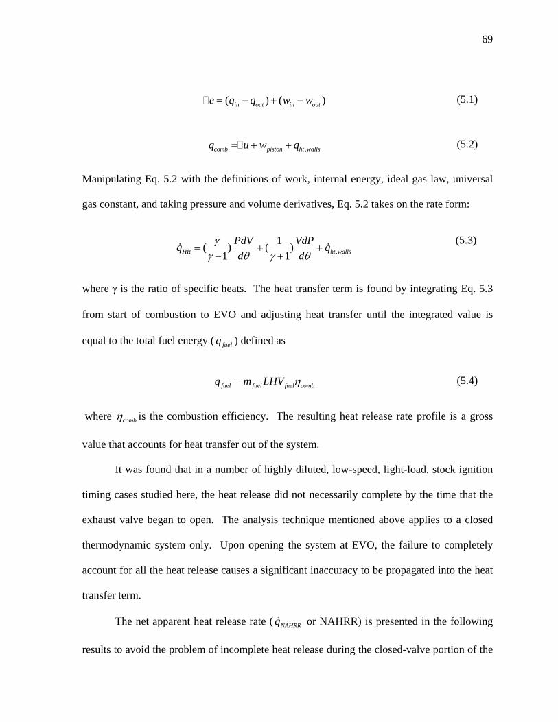
69
( ) ( )in out in oute q q w w= − + − (5.1)
,comb piston ht wallsq u w q= + + (5.2)
Manipulating Eq. 5.2 with the definitions of work, internal energy, ideal gas law, universal
gas constant, and taking pressure and volume derivatives, Eq. 5.2 takes on the rate form:
.1( ) ( )
1 1HR ht wallsPdV VdPq qd d
γγ θ γ θ
= + +− +
& & (5.3)
where γ is the ratio of specific heats. The heat transfer term is found by integrating Eq. 5.3
from start of combustion to EVO and adjusting heat transfer until the integrated value is
equal to the total fuel energy ( fuelq ) defined as
fuel fuel fuel combq m LHV η= (5.4)
where combη is the combustion efficiency. The resulting heat release rate profile is a gross
value that accounts for heat transfer out of the system.
It was found that in a number of highly diluted, low-speed, light-load, stock ignition
timing cases studied here, the heat release did not necessarily complete by the time that the
exhaust valve began to open. The analysis technique mentioned above applies to a closed
thermodynamic system only. Upon opening the system at EVO, the failure to completely
account for all the heat release causes a significant inaccuracy to be propagated into the heat
transfer term.
The net apparent heat release rate ( NAHRRq& or NAHRR) is presented in the following
results to avoid the problem of incomplete heat release during the closed-valve portion of the

70
cycle. The net heat release is the chemical heat release excluding the heat loss to the
combustion chamber surface.
The resulting equation for NAHRR is
1( ) ( )1 1NAHRR
VdP PdVqd d
γγ θ γ θ
= +− −
& (5.5)
The temperature-dependent γ from Gatowski et al. [28] was used in this work. For the cases
discussed below, the integrated heat release was always found to be less than the potential
chemical energy release of the fuel (accounting for the combustion efficiency and lower
heating value). The heat transfer accounts for this difference between chemical energy and
integrated heat release.
5.2.1 Emissions Index Calculations
Emissions indices are presented in this work for direct comparison of emissions
output with the values normalized to fuel consumption. Emissions index is defined by the
mass of the pollutant divided by the mass of fuel, Eq 5.6.
[ / ][ / ]
pol
fuel
m g sEI
m kg s=
&
&
(5.6)
The method used to arrive at the emissions index for NOx, HC, and combined (NOx + HC)
utilizes the measured emissions data, air flow rate, and A/F ratio. The first step manipulates
the carbon balance to allow the total moles of exhaust to be determined ( exhn ). Equation 5.7
defines the carbon balance on a per mole of fuel, per carbon atom basis. Here (y) defines the
hydrogen to carbon ratio.

71
2yCH CO CO HCn n n n= + + (5.7)
The number of moles of pollutant species, Eq. 5.8, is defined from the product of measured
mole fraction and total number of exhaust moles.
exhexhpolpol npolnn100
][== χ (5.8)
By substituting equation 5.8 into equation 5.7 for each of the three species, the total moles of
exhaust on a per mole of fuel basis takes the form of Eq. 5.9.
][][][100
2 HCCOCOnexh ++
= (5.9)
This analysis assumes all involved species concentrations were reported as a percentage of
volume flow over total volume flow which is equal to the species mole fraction. As
described in section 4.4,”wet” and “dry” measurements and appropriate corrections must be
applied. Exhaust moles will be “dry” when all of these species are measured “dry”.
Equation (5.10) and (5.11) are used for conversion in the same fashion described in
section 4.4.
exhOHdryexh
dryexhEXH nn
nK
,,
,
2+
= (5.10)
dryEXHwet polKpol ][][ = (5.11)
The mass flow of the pollutant ( polm& ) can be determined from Eq. 5.12, taken from
[29].

72
timen
nn
nm
nn
m fuel
fuel
exh
pol
pol
exh
polpol =&
(5.12)
In Eq. 5.12, substitutions for each of the four terms following the equal sign may be made as
follows: measured mole fraction, molecular weight of the pollutant, moles of exhaust from
Eq. 5.9 per one mole of fuel, and molar flow rate of fuel ( , /
y
fuel g s
CH
mMW
&). This yields the
following equation:
( )pol pol exh pol fuel fuel,gm x n MW /MW m= ⋅ ⋅ ⋅& & (5.13)
Finally, dividing Eq. 5.13 by the fuel mass flow rate in kg/s delivers the emissions index
value.
5.3 Comparison of Fuel Delivery System
Examining the fuel delivery systems foremost identifies any performance and
emissions effects caused by mixture preparation quality. For a given operating condition
with no additional EGR, only minimal differences exit in measured internal residual as seen
in Figure 5.1. Figure 5.2 compares the average IMEP for the two fuel systems at each load
condition. These slight differences in IMEP and residual are attributed to throttle position
differences observed when manually targeting specific load.

73
0.4
0.3
0.2
0.1
0.0
y dilu
ent -
Car
b
0.40.30.20.10.0ydiluent- HMS
Figure 5.1: Comparison of measured in-cylinder residual for each condition with the carburetor and HMS fuel systems. Presented data contains no EGR, both stock and maximum overlap cam, and stock and optimized ignition timing at all speeds and loads.

74
300
250
200
150
100
IMEP
[kPa
] - C
arb
300250200150100IMEP [kPa] - HMS
Figure 5.2: Comparison of IMEP for each condition with the carburetor and HMS fuel systems. Presented data contains no EGR, both stock and maximum overlap cam, and stock and optimized ignition timing at all speeds and light-loads.
The effects of the fuel system were found to be relatively small in regards to
combustion quality and emissions output at most conditions. A comparison of performance
and emissions output follows.
5.3.1 Fuel Preparation Effects on Combustion Performance
A slight bias towards longer burn durations was found for the carburetor compared to
the HMS in a number of instances, see Figure 5.3. This bias does not exist for all cases and
is, in all but a few instances, within 5 crank angle degrees, as shown in Figure 5.4.
Looking closer at the net apparent heat release rate profiles at light-loads, Figure 5.5,
reveals that the two fuel systems offer similar burn rates throughout combustion. Only at

75
light-load conditions, Figure 5.5 a) and b), does the HMS appear to offer slightly earlier peak
burn rate. Referring back to Figure 5.4 shows no real dependence exists between burn
duration of the two fuel systems and speed or load.
80
70
60
50
40
30
2010%
to 9
0% B
urn
Dur
atio
n [C
A d
eg] -
Car
b
8070605040302010% to 90% Burn Duration [CA deg] - HMS
Figure 5.3: Comparison of 10% to 90% burn duration at each condition with the carburetor and HMS fuel systems.

76
25
30
35
40
45
50
55
60
65
70
75
1750
rpm
- 10
% -
stk.
cam
- ad
v. ig
n.
1750
rpm
- 10
% -
max
. cam
- ad
v. ig
n.
1750
rpm
- 10
% -
stk.
cam
- st
k. ig
n.
1750
rpm
- 10
% -
max
. cam
- st
k. ig
n.
1750
rpm
- 25
% -
stk.
cam
- ad
v. ig
n.
1750
rpm
- 25
% -
max
. cam
- ad
v. ig
n.
1750
rpm
- 25
% -
stk.
cam
- st
k. ig
n.
1750
rpm
- 25
% -
max
. cam
- st
k. ig
n.
3060
rpm
- 10
% -
stk.
cam
- ad
v. ig
n.
3060
rpm
- 10
% -
max
. cam
- ad
v. ig
n.
3060
rpm
- 10
% -
stk.
cam
- st
k. ig
n.
3060
rpm
- 10
% -
max
. cam
- st
k. ig
n.
3060
rpm
- 25
% -
stk.
cam
- ad
v. ig
n.
3060
rpm
- 25
% -
max
. cam
- ad
v. ig
n.
3060
rpm
- 25
% -
stk.
cam
- st
k. ig
n.
3060
rpm
- 25
% -
max
. cam
- st
k. ig
n.
3060
rpm
- W
OT
- stk
. cam
- ad
v. ig
n.
3060
rpm
- W
OT
- max
. cam
- ad
v. ig
n.
3060
rpm
- W
OT
- stk
. cam
- st
k. ig
n.
3060
rpm
- W
OT
- max
. cam
- st
k. ig
n.
10%
- 90
% B
urn
Dur
atio
n
carb
HMS
Figure 5.4: Comparison of 10% to 90% burn duration at each condition with the carburetor and HMS fuel systems. Each condition in listed across the abscissa.
a)
4
3
2
1
0
NAH
RR
[J/d
eg]
80400-40CA [deg]
HMS, stk. cam, stk. ign. HMS, max OL cam, stk. ign. Carb, stk. cam, stk. ign. Carb, max OL cam, stk. ign
b)
80400-40CA [deg]
c)
80400-40CA [deg]
Figure 5.5: Net apparent heat release rates for carburetor and HMS at three speed/load conditions; a) 1750 rpm - 10% load, b) 3060 rpm – 10% load, c) 3060 rpm – 25% load. Only the stock ignition timing cases are shown here since ignition timing could be different between the carburetor and HMS when timing was optimized.

77
A final comparison between the combustion performance of the carburetor and the
HMS looks at variations in IMEP over 500 cycles. Figure 5.6 show a strong bias towards
higher COV of IMEP for the carburetor. The bias appears random with regards to level of
COV. At low-speed, light-load conditions difficulties in maintaining steady operating speed,
constant A/F, and target load with the carburetor were experienced. The unsteady nature
occurred in a periodic fashion with the A/F becoming very rich, engine slowing, and torque
decreasing followed by a swing towards lean conditions, increased engine speed, and
increased engine torque. Using the HMS system avoided this periodic swing in operating
parameters and produced significantly more stable steady-state operation.
25
20
15
10
5
0
CO
V of
IMEP
- C
arb
2520151050COV of IMEP - HMS
Figure 5.6: Comparison of COV of IMEP at each condition with the carburetor and HMS fuel systems.

78
Examining a cycle dependence plot of IMEP for the Nth+1 cycle against IMEP for the
Nth cycle shows no strong prior cycle effect for either the carburetor of the HMS, Figure 5.7.
Greater cycle-to-cycle randomness can be noted with the carburetor with the outlying points
suggesting that a strong cycle can be followed by a weak cycle or vice versa. This supports
the increased COV of IMEP reported with the carburetor.
a)180
160
140
120
100
80
60
IME
P N
+1 [k
Pa]
1801601401201008060IMEP N [kPa]
b)180
160
140
120
100
80
60
IME
P N
+1 [k
Pa]
1801601401201008060IMEP N [kPa]
Figure 5.7: IMEP cycle dependence for a) carburetor and b) HMS at 1750rpm, 10% load, stock cam, and stock ignition.
5.3.2 Fuel Preparation Effects on Engine-Out Emissions
Most operating conditions produced similar NOx and HC emissions between the
carburetor and the HMS. However, a bias towards higher HC with the carburetor, as seen in
Figure 5.8, is attributed to the periodic swing to very rich A/F at low-speed, light load
conditions. While one-minute averaged values of A/F were maintained at 12.0±0.5:1 with
the carburetor, it was noted that these swings occasionally reached as rich as 9.5:1. Figure
5.9 shows the EIHC as a function of A/F for both carburetor and HMS. The EIHC for the

79
carburetor tends to increase as the A/F decreases. The HMS maintains much more accurate
A/F and avoids this trend altogether; however, some high levels of HC occur at 12.0:1 due to
poor combustion as discussed in the following sections.
It is for this reason that the data presented in the remaining section of this Chapter
will focus on HMS data since A/F ratio was maintained very close to target and showed no
signs of instability. By using the HMS data, the phenomena presented hereafter shall avoid
misrepresentation from the influence of A/F fluctuations.
100
80
60
40
20
0
EIH
C [g
/kg f
uel]
- C
arb
100806040200EIHC [g/kgfuel] - HMS
Figure 5.8: Comparison of unburned hydrocarbon emission index for the carburetor and HMS at corresponding conditions.
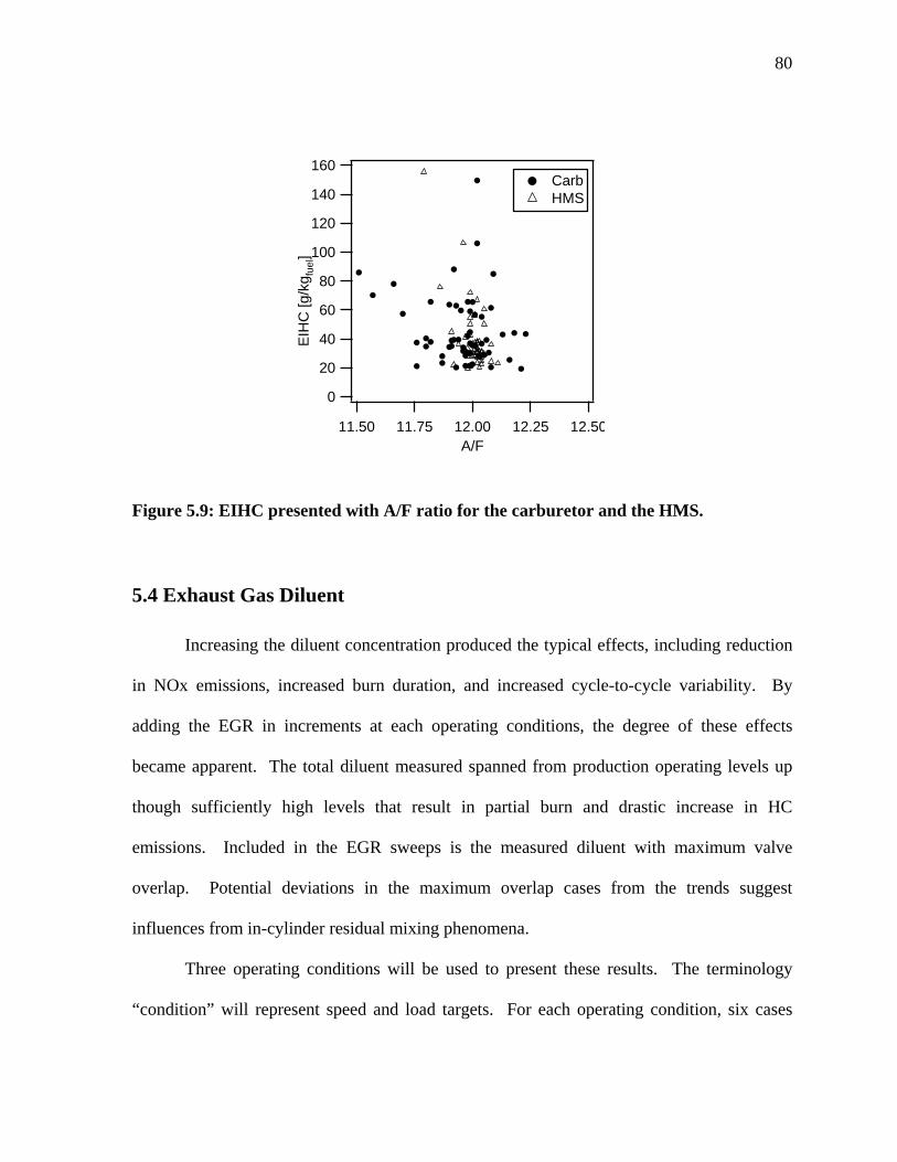
80
160
140
120
100
80
60
40
20
0
EIH
C [g
/kg f
uel]
12.5012.2512.0011.7511.50A/F
Carb HMS
Figure 5.9: EIHC presented with A/F ratio for the carburetor and the HMS.
5.4 Exhaust Gas Diluent
Increasing the diluent concentration produced the typical effects, including reduction
in NOx emissions, increased burn duration, and increased cycle-to-cycle variability. By
adding the EGR in increments at each operating conditions, the degree of these effects
became apparent. The total diluent measured spanned from production operating levels up
though sufficiently high levels that result in partial burn and drastic increase in HC
emissions. Included in the EGR sweeps is the measured diluent with maximum valve
overlap. Potential deviations in the maximum overlap cases from the trends suggest
influences from in-cylinder residual mixing phenomena.
Three operating conditions will be used to present these results. The terminology
“condition” will represent speed and load targets. For each operating condition, six cases

81
were tested. The first case, referred to as case “1”, used the stock cam timing and no external
EGR. Cases “2 – 5” used increasing levels of EGR. Finally, a case was run with no EGR,
but maximum valve overlap (128 degrees) to achieve higher internal residual gas retention
and is referred to as case “m”. The trapped diluent mass fraction and EGR mass fraction are
given in Table 5.1 for each of the cases tested.
Table 5.1: Trapped diluent fraction and external EGR rate for the tested conditions
Condition
1750 rpm
10% load
3060 rpm
10% load
3060 rpm
25% load
ydil yEGR ydil yEGR ydil yEGR 1 0.19 0.00 0.14 0.00 0.11 0.00 2 0.25 0.09 0.16 0.03 0.13 0.03 3 0.26 0.11 0.18 0.06 0.15 0.04 4 0.28 0.15 0.19 0.07 0.16 0.06 5 0.37 0.27 0.28 0.18 0.25 0.16
Cas
e
m 0.34 0.00 0.21 0.00 0.18 0.00 Note: case “1” diluent fraction does not remain constant as EGR is added since
throttling and mass flow change throughout the EGR sweeps.
5.4.1 Effects on Combustion Performance
The degree to which EGR influences the heat release profile reaches a critical level
when a fraction of the charge has yet to burn. Figure 5.10 shows the NAHRR for the 1750
rpm, 10% load case, stock ignition timing conditions. The baseline case, “1”, completes
combustion at about 70 aTDC, but the maximum overlap case and case “5” still have not

82
completed combustion by 100 aTDC (close to EVO). In fact, at about 90 aTDC cases 5 and
“m” show an inflection point that is considered to be the very beginning of exhaust valve
opening. Cases “2, 3 and 4” are very close to one another, but they follow a progression with
the highest of these three, diluent case “4”, having the longest combustion duration.
3
2
1
0
NA
HR
R [J
/deg
]
80400-40CA [deg]
Figure 5.10: Net apparent heat release rate for the stock ignition timing for 1750 rpm and 10% load. Bold line, case 1; red line, case 2; blue line, case3; green line, case 4; dashed line, case 5; dotted line, maximum overlap.
The other two conditions, shown in Fig. 5.11, follow the same trends, with the
increase in diluent fraction causing a lower peak heat release rate and the possibility of heat
release continuing to the point of exhaust valve opening. This trend is followed closely while
maintaining 10% load and increasing the speed to 3060 rpm, Figure 5.11 a); however,
increasing the load at 3060rpm, Figure 5.11 b), improves burn duration resulting in complete

83
heat release for most cases. The improvements with increased load are not sufficient for the
highly diluted cases “m” and “5”to force complete heat release before EVO.
a)3
2
1
0
NAH
RR
[J/d
eg]
80400-40CA [deg]
b)5
4
3
2
1
0N
AHR
R [J
/deg
]
80400-40CA [deg]
Figure 5.11: Net apparent heat release rate for the stock ignition timing for (a) 3060 rpm and 10% load, (b) 3060 rpm and 25% load (note vertical axis scale). Bold line, case 1; red line, case 2; blue line, case3; green line, case 4; dashed line, case 5; dotted line, maximum overlap.
Figure 5.12 shows the relation between peak pressure and the location of peak
pressure for the 3060 rpm, 10% load condition. Case “1”through “5” and “m”, are shown in
progressing order. The peak pressure for each of the 500 averaged cycles in all cases are
well within the ‘hook-back” region [20]. As additional EGR is added, the data span a smaller
range of peak pressure location occurring closer to TDC. Both of these characteristics
indicate a very low burn rate. The peak pressure approaches the motoring pressure at high
diluent levels suggesting that combustion is in the very early stages of flame growth, with

84
small amounts of the charge having burnt. The case 1 data span a wider range of peak
pressure location indicating a range of combustion rates.
Two observations should be noted at this time; 1) the pressures are higher in case 5
because the engine was throttled less to achieve the same load, 2) The fixed spark timing
presented here is the same as production timing, which, at wide open throttle operation the
heat release rate is considerably higher, and the timing is close to MBT.
1)
1400
1200
1000
800
600
PkP
r [kP
a]
2) 3)
4)
1400
1200
1000
800
600
PkP
r [kP
a]
403020100-10 CA [deg]
5)
403020100-10 CA [deg]
m)
403020100-10 CA [deg]
Figure 5.12: Peak Pressure vs. Location of Peak Pressure for 6 cases, indicated at upper left of graph, at 3060 rpm and 10% load.
The plots in Figure 5.12 capture only the variation in peak pressure and express
nearly the opposite of the phenomena seen in variations in IMEP. The peak pressure and its

85
location appear to group closer together as greater amount of residual are present during
combustion; however, the late combustion phasing of the highly diluted cases, as shown in
Figures 5.10-11, causes significant variations later in the expansion stroke. Figure 5.13
shows IMEP of the (Nth+1) cycle against the Nth cycle. Besides displaying the variation from
one cycle to another, cycle dependence, such as weak cycles followed by strong cycles, can
be extracted from these plots. The obvious observation is that the spread in IMEP increases
with increasing diluent. There is no suggestion of cycle-to-cycle dependence from these data
due to the pure randomness of the proceeding cycle for any one cycle. The trends displayed
in Figures 5.12 and 5.13 were seen for all operating conditions.

86
1) 250
200
150
100
50
IMEP
N+1
[kP
a]2) 3)
4) 250
200
150
100
50
IME
P N
+1 [k
Pa]
25020015010050 IMEP N [kPa]
5)
25020015010050 IMEP N [kPa]
m)
25020015010050 IMEP N [kPa]
Figure 5.13: IMEP for cycle N+1 versus IMEP for cycle N for 6 cases, indicated at upper left of graph, at 1750 rpm and 10% load.
5.4.2 Effects on Engine-Out Emissions
The effect of diluent on emissions, HC+NOx being of greatest interest, can be seen in
Fig. 5.14 for the three conditions discussed above. Also shown on the right ordinate in Fig. 6
are the COV of IMEP data. The best fit lines have been added for visual reference. The
increase in combustion variability with increasing diluent shown in Figure 5.13 is
summarized here with COV of IMEP.

87
a)
60
50
40
30
20
10
0
EI(N
Ox+
HC
) [g/
kgfu
el]
0.400.300.200.10
ydil
60
50
40
30
20
10
0
CO
V IM
EP[%
]
1234
m
1 234
5m
5 @ (0.37,106)
b)
60
50
40
30
20
10
0
EI(N
Ox+
HC
) [g/
kgfu
el]
0.400.300.200.10ydil
60
50
40
30
20
10
0
CO
VIM
EP [%
]
1234
5
m
1234
5m
c)
60
50
40
30
20
10
0
EI(N
Ox+
HC
) [g/
kgfu
el]
0.400.300.200.10
ydil
60
50
40
30
20
10
0
CO
VIM
EP [%
]
12345
m
1234
5m
Figure 5.14: Emissions and combustion variability for stock ignition conditions (a) 1750 rpm and 10% load, (a) 3060 rpm and 10% load, (a) 3060 rpm and 25% load. Numbered points refer to the EGR cases of Table 5.1.
The emissions data show that there is an optimum level of diluent that minimizes the
HC+NOx emissions, with the minimum occurring at a different diluent level based on
operating condition. As the diluent level increases the NOx emissions reduce, but referring
to Fig. 5.15, the NOx emissions are a small portion of the HC+NOx emissions at these light-

88
load conditions. Thus, the reduction is HC+NOx is dominantly driven by a reduction in HC
emissions. The initial HC reduction may be attributed to both a ‘reburning’ of the HC in the
residual within the combustion chamber and a reduction in crevice hydrocarbons due to the
lower in-cylinder pressures. At a point, however, this effect is overwhelmed by a reduction
in combustion quality, and the HC emissions rapidly increase as a function of diluent.
5
4
3
2
1
EIN
Ox
[g/k
g fue
l]
0.300.250.200.150.10
ydil
1
234
5m
Figure 5.15: NOx emissions index as a function of trapped diluent fraction at 3060 rpm and 25% load. Numbered points refer to the EGR cases of Table 5.1.
An overall objective of this work was to investigate at what level elevated residual
fraction begins to impact engine emissions. Therefore, cases that were near, and just beyond
the minimum HC+NOx levels were investigated in further detail. Initially, it was perceived
that beyond some specific COV of IMEP the HC emissions would undergo a drastic increase.
However, examining the linearly increasing COV of IMEP trend against the parabolic HC
data, the COV of IMEP was found to be a poor indicator of the significant increase in HC
emissions. For example, at 1750 rpm and 10% load, a diluent fraction of approximately 25%
gave the lowest combined emissions, and at that condition the COV of IMEP was 10%.

89
However, at 3060 rpm and 10% load least emissions occurred at 20% diluent, where the
COV of IMEP was about 15%.
To directly assess whether combustion quality was adversely affecting the HC
emissions, the cycle-resolved HC data from the fast FID were interrogated on a cycle-by-
cycle basis, and compared to the preceding combustion event quality, assessed by the IMEP.
Three crank angle timings were investigated, 130, 225 and 360 aTDC, to represent the
blowdown process, the main exhaust event, and the crevice gas release period, respectively.
These three events are described with greater detail in Section 2.4.3. Figure 5.16 displays the
FFID output trace for each case averaged over 500 cycles at 1750 rpm and 10% load. Cycle-
by-cycle values provide greater information in regards to the influence of combustion quality
on emissions compared to these averaged traces so plots like that in Figure 5.16 have limited
use in this discussion.

90
10000
8000
6000
4000
2000
0
HC
[ppm
C3]
540450360270180900-90-180CA [deg]
Figure 5.16: Averaged FFID output traces at 1750 RPM and 10% load. Bold line, case 1; red line, case 2; blue line, case3; green line, case 4; dashed line, case 5; dotted line, maximum overlap.
Figure 5.17 shows the HC concentration at the 130 aTDC position, FFID1, as a function
of the cycle IMEP for one case near the combined emissions minima (left column), one case
just past the minima, or in a region where combustion quality is thought to be affecting the
HC emissions (middle column), and one case with the greatest amount of diluent. These
three events were captured in case “4”, “m”, and “5” for each of the operating conditions.
The premise of these plots is that a poor combustion event with incomplete combustion likely
and partial oxidation of the fuel would increase levels of hydrocarbon emissions.
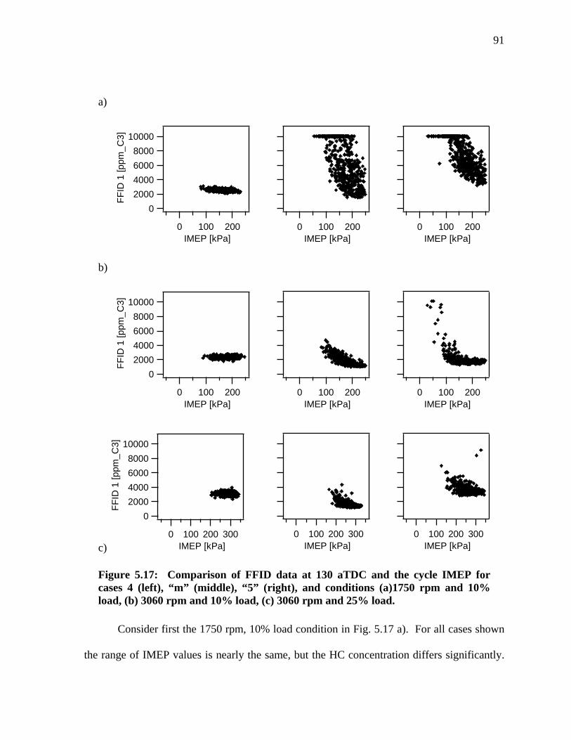
91
a)
100008000600040002000
0 FFI
D 1
[ppm
_C3]
2001000 IMEP [kPa]
2001000 IMEP [kPa]
2001000 IMEP [kPa]
b)
100008000600040002000
0 FFI
D 1
[ppm
_C3]
2001000 IMEP [kPa]
2001000 IMEP [kPa]
2001000 IMEP [kPa]
c)
100008000600040002000
0 FFI
D 1
[ppm
_C3]
3002001000 IMEP [kPa]
3002001000 IMEP [kPa]
3002001000 IMEP [kPa]
Figure 5.17: Comparison of FFID data at 130 aTDC and the cycle IMEP for cases 4 (left), “m” (middle), “5” (right), and conditions (a)1750 rpm and 10% load, (b) 3060 rpm and 10% load, (c) 3060 rpm and 25% load.
Consider first the 1750 rpm, 10% load condition in Fig. 5.17 a). For all cases shown
the range of IMEP values is nearly the same, but the HC concentration differs significantly.

92
The case “4” data show very little variation in HC concentration with respect to IMEP.
However, the case “m” and “5”data show a strong inverse correlation between HC
concentration and IMEP, indicating that indeed low IMEP cycles are resulting in high HC
emissions.
The 1750 rpm, 10% load operating condition has a rather large change in diluent
fraction, 0.28 to 0.34 to 0.37, from case “4” to “m” to “5”, respectively; however, the other
two operating conditions shown in Figures 5.17 b) and c) have much less difference in
diluent fraction. For both the 3060 rpm 10% and 25% load conditions, the case “4” and case
“m” conditions have less than 3% difference in the trapped diluent fraction, and the
HC+NOx, Figure 5.14, emissions are very similar. From case “m” to case “5” there is a 7%
increase in the trapped diluent fraction, and the HC+NOx emissions are significantly greater
with case “5”, especially at 3060 rpm and 10% load. The range of individual-cycle IMEP is
comparable for the optimal, post-optimal, and greatest diluent cases. There is, however, a
substantial difference between the HC – IMEP correlation. The case 4 conditions show no
correlation between the HC concentration at 130 aTDC and IMEP for any of the cases,
suggesting that at these conditions the combustion does not affect the HC emissions. The
case “m” conditions show an upward sweeping increase in HC concentration at low IMEP,
indicating that the combustion quality has begun to impact the HC emissions. Case “5”
conditions show that the spread in HC emissions has moved up while the upward sweeping
increase becomes more pronounced. The data of Figure 5.17 prove that above a critical level
of dilution, the reduction in combustion quality does affect the HC emissions.
A more detailed look at the data reveals that the onset of the negative correlation
between the FFID results and the cycle IMEP, i.e. when the combustion quality is beginning

93
to adversely affect emissions, occurs at the time when the heat release is still occurring at
EVO. Referring back to Figure 5.10 and 5.11 b), the case “4” heat release data are seen to
reach zero at 100 aTDC, and the case “5” and “m” data are clearly positive at EVO.
Likewise, the case “5” and “m” in Fig. 5.17 show the negative HC – IMEP correlation. The
3060 rpm, 10% load heat release data deviate slightly from this trend, with all of the heat
release data, except case 1, positive at 100 aTDC.
The correlation with IMEP did not vary appreciably between the three FFID events,
as seen in Figure 5.18; however, a slight reduction in the negative HC – IMEP correlation
occurs by FFID 3. Any cycle experiencing incomplete heat release at EVO is believed to
expel higher concentrations of HC at the FFID 1 window due to the likeliness that the flame
front has not reached all combustion chamber walls before the blowdown occurs. The bulk
of the exhaust gas is considered to exit with concentrations represented at the FFID 2
window. Referring to Figure 5.16, at FFID 3 the majority of the gases have been evacuated
leaving only the HC that are normally expelled from piston ring crevice volumes.

94
a) FFID1
100008000600040002000
0 FFI
D 1
[ppm
_C3]
2001000 IMEP [kPa]
FFID2
2001000 IMEP N [kPa]
FFID3
2001000 IMEP [kPa]
b)
100008000600040002000
0 FFI
D 1
[ppm
_C3]
2001000 IMEP [kPa]
2001000 IMEP N [kPa]
2001000 IMEP [kPa]
c)
100008000600040002000
0 FFI
D 1
[ppm
_C3]
2001000 IMEP [kPa]
2001000 IMEP N [kPa]
2001000 IMEP [kPa]
Figure 5.18: Comparison of three FFID points 130 aTDC (left), 225 aTDC (middle), and TDC (right) throughout the exhaust cycle at 3060 rpm, 10% load, case a) “4”, b) “m”, and c) “5”.

95
5.5 Ignition Timing Effects
A simple procedure was followed to optimize the ignition timing at all the conditions
investigated, similar to the work by [8]. The target load was reached with stock ignition
timing. The spark timing was then advanced until the torque reached a maximum, then the
throttle was readjusted to reestablish the target load. In this manner an ignition timing close
to MBT, and considerably advanced from the stock timing, was achieved for each condition.
The trapped diluent mass fraction and EGR mass fraction are given in Table 5.2 for
each of the cases tested with optimized ignition. It should be noted that the diluent fractions
are higher in these studies in comparison to stock timing diluent, Table 5.1, since the
advanced combustion yields greater time for heat transfer out of the combustion chamber
resulting in lower temperatures and higher density at the end of the exhaust stroke during the
overlap period.
Table 5.2: Trapped diluent fraction, external EGR rate, and spark timing for the optimized ignition conditions presented here.
Condition 1750 rpm
10% load
3060 rpm
10% load
3060 rpm
25% load
ydil yEGR Spark [bTDC] ydil yEGR Spark
[bTDC] ydil yEGR Spark [bTDC]
1 0.24 0 45 0.16 0 34 0.13 0 38 2 0.27 0.06 48 0.19 0.04 40 0.16 0.04 44 3 0.31 0.12 51 0.23 0.09 45 0.18 0.07 50 4 0.34 0.21 55 0.24 0.09 47 0.19 0.08 53 5 0.46 0.37 63 0.35 0.23 59 0.31 0.19 57
Cas
e
M 0.38 0 57 0.28 0 47 0.23 0 49

96
5.5.1 Ignition Timing Effects on Combustion Performance
Significant improvements in heat release rate, combustion phasing, and cyclic
variability are seen in the optimized ignition study. Figure 5.19 shows heat release rates for
both the stock timing and optimized timing at 1750 rpm and 10% load. Advancing the
timing at this condition from 19 bTDC to between 45 bTDC for case “1” and 63 bTDC for
case “5” kept peak heat release rates near 15 aTDC as opposed to 30 to 40 aTDC as observed
with stock ignition timing. The heat release data for optimized ignition timing at 3060 rpm
10% and 25% loads is shown in Figure 5.20. Again, much improvement is noted in regards
to combustion phasing and heat release rate.
Examining the peak pressure and location of peak pressure, Figure 5.21, further
demonstrates the improvements in combustion quality. With stock timing, adding EGR
continually forced slower heat release, therefore, moving the peak pressure and location
towards motored pressure, Figure 5.12. Optimizing the timing returns the peak pressure to a
more

97
optimal location for each case, i.e. further up the hook-back region as described by
[Matekunas]. Figure 5.21 shows peak pressure versus location of peak pressure for all six
optimized ignition timing cases 3060 rpm, 10% load. Compared to Figure 5.12, the peak
pressure with optimized ignition remains well within the same hook-back region for all cases
or seemingly independent of diluent fraction. Not until the very high levels of diluent as in
case “5” and case “m”, does an appreciable push towards later phasing occur. All conditions
shared this trend where only highly diluted cases began to show later phasing with the
optimized ignition.
3
2
1
0
NAH
RR
[J/d
eg]
80400-40CA [deg]
3
2
1
0
NAH
RR
[J/d
eg]
80400-40CA [deg]
Figure 5.19: Net apparent heat release rate for the a) stock ignition timing and b) optimized ignition timing for 1750 rpm, 10% load. Bold line, case 1; red line, case 2; blue line, case3; green line, case 4; dashed line, case 5; dotted line, max. overlap.

98
3
2
1
0
NAH
RR
[J/d
eg]
80400-40CA [deg]
5
4
3
2
1
0
NAH
RR
[J/d
eg]
80400-40CA [deg]
Figure 5.20: Net apparent heat release rate for the optimized ignition timing for (a) 3060 rpm and 10% load, (b) 3060 rpm and 25% load (note vertical axis scale). Bold line, case 1; red line, case 2; blue line, case3; green line, case 4; dashed line, case 5; dotted line, maximum overlap.
Additional improvements can be noted in the cycle-to-cycle variations in IMEP when
the timing was optimized, see Figure 5.22. Similar trends to those described above are seen
here where only highly diluted cases experience noticeable change. Case “5” and “m” show
significant increase in cycle-to-cycle IMEP variations. The stock timing showed a steady
increase in cyclic IMEP scatter as EGR was added while the optimized ignition cases show
very little degradation in cyclic IMEP with the increasing EGR until significant levels in
diluent fraction are reached. For example, at 1750 rpm, 10% load, IMEP scatter begins to
increase when diluent fraction reaches about 0.35. Increasing the speed to 3060 rpm and
maintaining 10% load pushes this limit down around 0.30, below which combustion phasing
and cyclic stability show only slight degradation from case 1 to 4, as seen in Figure 5.22.

99
1)
1400
1200
1000
800
600
PkP
r [kP
a]2)
3)
4)
1400
1200
1000
800
600
PkP
r [kP
a]
403020100-10 CA [deg]
5)
403020100-10 CA [deg]
m)
403020100-10 CA [deg]
Figure 5.21: Peak Pressure vs. Location of Peak Pressure for 6 cases, indicated at upper left of graph, with individually optimized ignition timing at 3060 rpm and 10% load.

100
1) 250
200
150
100
50
IMEP
N+1
[kPa
]
2) 3)
4) 300
250
200
150
100
50
IMEP
N+1
[kP
a]
25020015010050 IMEP N [kPa]
5)
25020015010050 IMEP N [kPa]
m)
25020015010050 IMEP N [kPa]
Figure 5.22: IMEP for cycle N+1 versus IMEP for cycle N for 6 optimized ignition cases, indicated at upper left of graph, at 1750 rpm and 10% load.
5.5.2 Ignition Timing Effects on Engine-Out Emissions
Relevant to the discussion in Section5.4.2, at the 1750 rpm, 10% load and 3060
rpm, 10% load conditions the heat release is completed at 100 aTDC for all of the cases
except case “5” and case “m”, Figures 5.19 and 5.20 a). At the 3060 rpm, 25% load
condition, the heat release is completed at 100 aTDC for all of the six cases investigated as a
result of greater charge momentum associated with the increased load.

101
Figure 5.23 shows the correlation between the FFID data at 130 aTDC and the cycle IMEP
for the optimized ignition timing data. The three cases shown for each condition are case
“4”, case “m”, and case “5”. At the 1750 and 3060 rpm, 10 % load conditions, the case 4
data show no inverse correlation between HC concentration and IMEP. However, the case
“m’ data for these two cases do show a negative correlation. This is consistent with the
observation that the heat release at the “m” case extended to exhaust valve opening. For the
3060 rpm, 25% load condition all cases completed heat release prior to 130 aTDC, Figure
5.20 b), and no correlation is observed between the HC concentration at 130 aTDC and the
cycle IMEP.
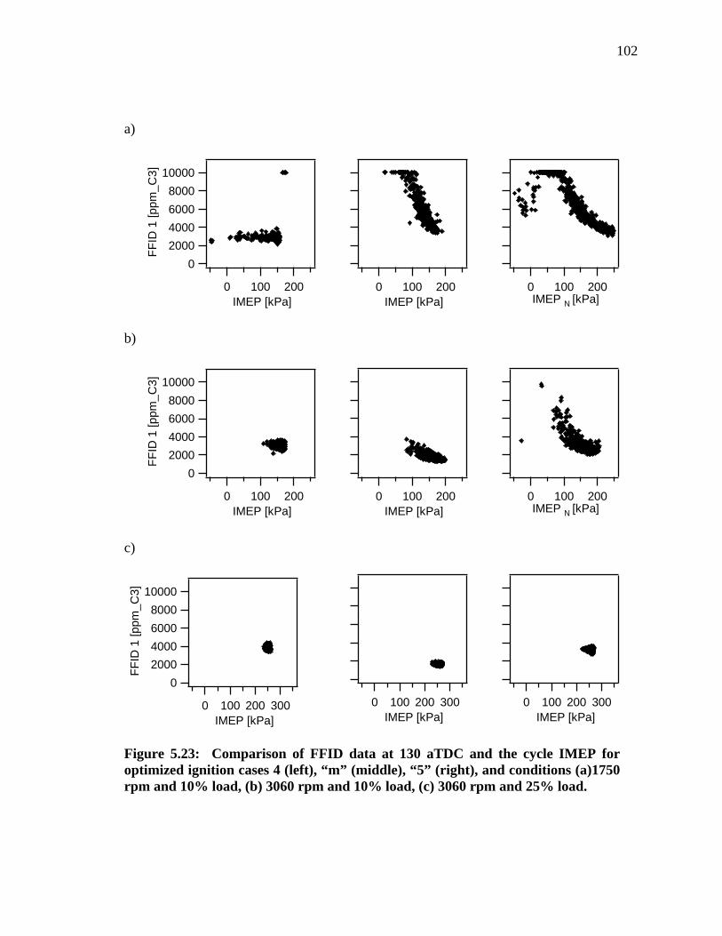
102
a)
100008000600040002000
0 FFI
D 1
[ppm
_C3]
2001000 IMEP [kPa]
2001000 IMEP [kPa]
2001000 IMEP N [kPa]
b)
100008000600040002000
0 FFI
D 1
[ppm
_C3]
2001000 IMEP [kPa]
2001000 IMEP [kPa]
2001000 IMEP N [kPa]
c)
100008000600040002000
0 FFI
D 1
[ppm
_C3]
3002001000 IMEP [kPa]
3002001000 IMEP [kPa]
3002001000 IMEP [kPa]
Figure 5.23: Comparison of FFID data at 130 aTDC and the cycle IMEP for optimized ignition cases 4 (left), “m” (middle), “5” (right), and conditions (a)1750 rpm and 10% load, (b) 3060 rpm and 10% load, (c) 3060 rpm and 25% load.
103
Examining the HC emissions index for the optimized ignition cases at these three
conditions, Figure 5.24, reveals similar trends to those with stock ignition shown in Figure
5.14. There exists a minimum in HC with the addition of some EGR. Beyond this minimum
the HC emissions begin to increase. A closer look at each operating condition shows good
agreement with the negative HC – IMEP data in Figure 5.23. At 1750 rpm, 10% load the HC
emissions are minimized near case “4”, which in Figure 5.23 shows no negative HC – IMEP
correlation. Case “m” shows a significant increase in HC emissions and the correlation has
become very prominent. The HC emissions reached 156 g/kg_fuel by case “5”, where in
Figure 5.23, this case shows that a significant number of poor cycles have saturated the FFID
suggesting strong negative correlation. It should be noted that the diluent fraction is 0.46 at
case “5”. At 3060 rpm, 10% load the tolerance to diluent and minimum emissions appears to
span a much greater range in dilution compared to stock ignition. Case “m” borders on the
maximum diluent fraction for minimum emissions while the FFID data supports this with the
negative HC – IMEP correlation just setting in. By case “5” HC emissions have increased
and the correlation is well established. There is no correlation at any case at 3060 rpm, 25%
load. This is consistent with the emissions data and heat release rate profile for this
condition.

104
a)
80
60
40
20
0
EI(N
Ox+
HC
) [g/
kgfu
el]
0.400.300.200.10
ydil
60
50
40
30
20
10
0
CO
VIM
EP [%
]
1 2 3 4
m
12 3
4m
5 @ (0.46,156)
b)
60
50
40
30
20
10
0
EI(N
Ox+
HC
) [g/
kgfu
el]
0.400.300.200.10
ydil
60
50
40
30
20
10
0
CO
VIM
EP [%
]
1 2 34
5
m
1 2 34
5m
c)
60
50
40
30
20
10
0
EI(N
Ox+
HC
) [g/
kgfu
el]
0.400.300.200.10
ydil
60
50
40
30
20
10
0
CO
VIM
EP [%
]
1 234 5m
1 234 5m
Figure 5.24: Emissions and combustion variability for stock ignition conditions (a) 1750 rpm and 10% load, (a) 3060 rpm and 10% load, (a) 3060 rpm and 25% load. Numbered points refer to the EGR cases of Table 5.1.
The stock and optimized ignition timing data provide a consistent conclusion
regarding the point where combustion instability brought on by elevated dilution levels
adversely affects the engine emissions. For both stock and optimized ignition, the correlation
between increased HC concentration in the exhaust just after exhaust valve opening and the

105
cycle IMEP became prevalent when the heat release was found to extend beyond exhaust
valve opening.
There are some other interesting features of the optimized ignition timing that merit
comment aside from improved the combustion quality, reduced heat release duration, and
optimized combustion phasing. Looking at case “4” at 1750 rpm, 10% load in Figure 5.23
shows an interesting result during misfires, or cycles with negative IMEP. It is expected that
a misfire would result in a very high HC concentration for that cycle, but low HC is seen here
during the misfires. The cause for this behavior is believed to be that on the misfire cycle the
cylinder pressure is actually lower than the exhaust port pressure at EVO, causing backflow
into the cylinder. It was confirmed that shortly into the exhaust stroke the fast FID detector
saturated at the upper end of the output range, and this high concentration persisted in the
detector into the start of the following cycle. This cycle was strong due to the large fuel
content within the residual following the misfire; therefore, the high HC concentrations
appear at the upper end of the IMEP range.
The improvements in the combustion brought about by the advanced ignition timing
suggest that it may be a good strategy for improved performance. A comparison of the
results in Figure 5.24 to those in Figure 5.14 show that the HC+NOx emissions actually
increase with the optimized ignition timing. This is considered to be a result of the increased
NOx production due to the higher in-cylinder temperatures and pressures, as well as an
increased in HC emissions due to the impact of higher cylinder pressure on the ring pack and
crevice volume contribution to HC emissions.

106
5.6 Comparison of Well Mixed EGR and Maximum Overlap
From the data in this study, the difference between the well-mixed external exhaust
gas recirculation and purely internal residual appears to be slight. In Figures 5.14 and 5.25
the case “m” data fall close to the trend lines for the well-mixed EGR cases. Part of the
reason for this small difference is the significant internal residual at the light load conditions.
The case “1” data always has the lowest trapped diluent, but the value is a significant fraction
of the EGR cases. The EGR amount is assumed to be correct after the careful correction
described in Section 4.xx have been applied. Therefore, the remained of the diluent is
considered to be from internal residual retention. For most conditions tested the case “5”
EGR accounted for between 60 and 70% of the total diluent.
In addition to the large portion of internal residual, exact diluent targeting was not
reasonable with the experimental setup. For this reason, direct comparisons between the
maximum overlap, purely internal residual and partial EGR are not made. Case “4” always
has less diluent than case “m”, which has less diluent than case “5”. Qualitative comparisons
of peak pressure versus location of peak pressure, IMEP dependence, and HC – IMEP are
made here.
From the arguments presented in association with the data in Figures 5.12, 5.13, 5.17,
5.21, 5.22, and 5.23 there is typically a continued progression from case “4” to case “m” to
case “5”. The diluent for these cases has reached sufficient level to cause so much scatter in
the cycle-by-cycle data that no obvious winner in regards to performance exists. This
suggests that these parameters are not significantly influenced by mixture preparation at these
levels of diluent or operating conditions.
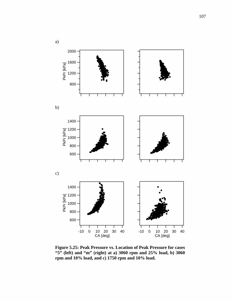
107
a)
2000
1600
1200
800
PkP
r [kP
a]
b)
1400
1200
1000
800
600
PkP
r [kP
a]
c)
1400
1200
1000
800
600
PkP
r [kP
a]
403020100-10 CA [deg]
403020100-10 CA [deg]
Figure 5.25: Peak Pressure vs. Location of Peak Pressure for cases “5” (left) and “m” (right) at a) 3060 rpm and 25% load, b) 3060 rpm and 10% load, and c) 1750 rpm and 10% load.

108
An interesting observation with optimized ignition timing deserves mention. In all
the optimized ignition conditions, case “5” was found to have about 8% greater total diluent
than case “m”; however, when the spark timing was advanced, case “5” tended to move up
the “hook-back” region further than case “m”. Figure 5.25 shows peak pressure versus
location of peak pressure for 1750 rpm, 10% load and 3060 rpm, 25% load cases “m” and
“5”. This is consistent with the heat release rate profiles for these cases in Figures 5.19 and
5.20 where the case “5” maximum heat release rate occurs earlier and with slightly greater
magnitude than case “m”. The optimum ignition timing for case “5” is 6, 12, and 8 degrees
further advance than case “m” for 1750 rpm and 10% load, 3060 rpm and 10% load, and
3060 rpm and 25% load, respectively. Although further advancement of the ignition in case
“m” may reduce this difference, loss in performance is expected beyond the reported spark
timing.
It may be inferred from Figure 5.25 that the combustion quality of the highly diluted
charge containing large amounts of premixed EGR was more easily restored with spark
advance than purely internal residual. It is believed that these differences may be a result of
in-cylinder conditions at ignition. With maximum overlap, EVC is delayed further into the
intake stroke, therefore, introducing greater residual later in the cycle. Additionally, spark
occurs very early in the compression stroke where a number of influential conditions on
flame development including low charge density, lower turbulence levels, and greater
likeliness of residual pockets from the reduced mixing time exist.
Using EGR with optimized ignition timing might suggest a means to improve
combustion performance; however, the observed increase in HC and NOx may advocate a
compromise between stock and MBT at light-load conditions with high levels of diluent.

109
5.7 Ignition Energy and Volume
As a compliment to optimizing the ignition timing, secondary studies were performed
on the spark energy and spark volume or gap at the most marginal operating condition, 1750
rpm and 10% load. Constant fuel and air flow was maintained throughout to observe any
effects on load. A sweep of energy extended from the lower combustion limit at which
regular misfires occurred and significant power loss was observed, up to the physical output
limitation of the coil. The spark gap was increased from its recommended width of 0.5 mm
to 1.0, 1.5, and 2.5 mm. At each gap a sweep through energy was performed. In this manner
a map demonstrating the minimum threshold and any possible improvements in combustion
quality was created.
The averaged NAHRR is shown in Figure 5.26 for four gaps, and two energy levels, 4
mJ and 50 mJ. The higher energy cases, shown in black, exhibit an earlier rise in heat release
for the wider gap cases, but in general no obvious trend can be observed. All cases show
similar magnitudes and peak rate location within 10 degrees CA with the exception of the
short gap, low energy case which appears to have slow burn characteristics.

110
2.0
1.5
1.0
0.5
0.0
NA
HR
R [J
/s]
100806040200-20-40CA [deg]
Figure 5.26: Net Apparent Heat Release Rate for 4 spark plug gaps; 2.5mm - bold solid line, 1.5mm - bold dashed line, 1mm - thin dashed line, 0.5mm – thin solid line, and two energy levels; 4.3 mJ - red, 50 mJ – black, at 1750 rpm, 10% load.
To further investigate the effects of ignition energy and gap, the peak pressure and
location of peak pressure from two energies and two gaps of the map are presented in Figure
5.27. Increasing the gap from 0.50 mm to 2.5 mm has a greater impact on moving the
pressure up the “hook-back” region than increasing the spark from 4.3 mJ up to 50 mJ. A
similar trend is noted when examining the cycle-to-cycle variations in Figure 5.28. Scatter is
noticeably reduced when the gap is increased, with a further tightening of cycle-to-cycle
IMEP occurring with the increase in spark energy. This may be attributed to the initial flame
kernel development being more consistent from cycle-to-cycle as a result of both greater

111
charge mass within the spark volume, and larger combustible gas fraction within the spark
volume.
a)
800
750
700
650
600
550
500
PkP
r [kP
a]
b)
c)
800
750
700
650
600
550
500
PkP
r [kP
a]
403020100-10 CA [deg]
d)
403020100-10CA [deg]
Figure 5.27: Peak Pressure versus location of peak pressure at 1750 rpm, 10% load for a) 4.3 mJ and 0.50 mm b) 4.3 mJ and 2.50 mm, c) 50 mJ and 0.50 mm, and d) 50 mJ and 2.50 mm.

112
a)
200
160
120
80 IMEP
N+1
[kPa
]
b)
c)
200
160
120
80 IMEP
N+1
[kPa
]
20016012080 IMEP N [kPa]
d)
20016012080 IMEP N [kPa]
Figure 5.28: IMEP for cycle N+1 versus IMEP for cycle N at 1750 rpm, 10% load for a) 4.3 mJ and 0.50 mm b) 4.3 mJ and 2.50 mm, c) 50 mJ and 0.50 mm, and d) 50 mJ and 2.50 mm.
The net effect of spark energy and volume on emissions is slight. Throughout most
of the range in spark energy and gap, the NOx + HC emissions index was constant between
35 and 40 g/kg fuel. Only at very low spark energies was a significantt increase in emissions
observed. The lowest energy tested was 1.75 mJ at 0.50 mm gap. Very poor combustion
quality was experienced and the reported emission index is near 80 g/kg fuel. Referring to
Figure 5.26, at 4.3 mJ and 0.50 mm gap the heat release rate extended farther than the other

113
cases, continuing to EVO. This is consistent with the increased emissions as seen in Figure
5.29. Also note in Figure 5.28 a) that a power loss was observed (the average IMEP was
lower than the other cases).
The NOx + HC emissions also show a rise at very high spark energies. The NOx
levels nearly doubled from about 1.5 g/kg fuel which is believed to be due to the large
amount of energy deposited from the spark into the combustion gases and electrode.
0 20 40 60 80 100 120 140
20
30
40
50
60
70
80
90
Espark [mJ]
EI(N
Ox+
HC
) [g
/kg f
uel ]
Figure 5.29: The NOx + HC emissions index for various spark energies and gaps of 0.5 mm (circles), 1.0 mm (squares), 1.5 mm(triangles), and 2.5 mm (bowties).
5.8 Intake Runner Volume Influence on Residual Retention
As described in Chapter 1 and 2, the mechanisms for residual retention in the small
utility engine environment differ from that of an automotive engine. In a multi-cylinder
engine considerable amounts of residual are drawn back into the intake during overlap from

114
the low manifold pressure at part load. This contribution to residual in small engines is much
less apparent.
A 1-D engine model was constructed early on in this project using GT-Power to
identify the amount of residual from three defined contributing factors: intake backflow,
clearance volume, and exhaust backflow. Residual fractions were predicted at part load
using a throttle controller to target measured IMEPs, see Figure 5.30. Mass flow across the
valves was analyzed during the overlap period to identify the direction of flow, and tp
calculate the fraction of residual flowing past the each of the valves. From this analysis it
was determined that 90% of the residual remains in the clearance volume during the overlap
period, while the remaining 10% is pulled back into the cylinder through the exhaust. Little
to no contribution was attributed to intake backflow.
0.25
0.20
0.15
0.10
0.05
0.00
y dil,
pred
icte
d
0.300.250.200.150.100.050.00ydil,measured
Figure 5.30: Comparison of predicted and measured residual fraction. GT-Power model of the Briggs Intek engine with optimized timing, stock camshaft, HMS used for prediction.

115
The purpose of this study was to determine the intake volume necessary to experience
a contribution from intake backflow in small engines. A number of intake volumes were
implemented, and the diluent fraction was measured at 1750 rpm at 10%, 25%, and 50%
load, and 3060 rpm at 10%, 25%, 50% and 100%. The intake volumes presented here are
normalized against the engine displacement volume.
Figure 5.31 displays the measured residual fraction as a function of normalized intake
volume for a) 1750 rpm and b) 3060 rpm. At 1750 rpm a slight increase in residual is seen as
the intake volume increases. The increase in residual fraction is greatest at 10% load from
0.21 up to 0.26. At 3060 rpm a peak in residual is observed for 10% and 25% loads near a
normalized volume of 3. Above this the measured residual decreases. Further examination
of the measured pressure during overlap provides details as to the flow potential across the
intake valve.

116
a)
0 1 2 3 4 5 60.05
0.1
0.15
0.2
0.25y d
il
Normalized Volume
b)
0 1 2 3 4 5 60.05
0.1
0.15
0.2
0.25
y dil
Normalized Volume
Figure 5.31: Measured residual as a function of normalized intake volume for a) 1750 rpm and b) 3060 rpm and 10% (circles), 25% (squares), 50% (triangles), and 100% (bowties).

117
The manifold absolute pressure (MAP) traces shown in Figure 5.32 show that at
sufficient volume the MAP fails to completely recover to atmospheric pressure before the
proceeding intake valve opening. Since the cylinder is considered to have equilibrated with
exhaust pressure near, or slightly above atmospheric pressure, the potential for backflow
across the intake valve exists. At 1750 rpm, 10% load a critical normalized volume, defined
qualitatively as having pressure slightly less that atmospheric at IVO near 335 CA°, was
found to be around 0.36. There was very little increase in the residual fraction at this point;
however, the next larger volume of 0.75 shows an increase consistent with the lower MAP at
IVO. Small difference in the critical volume was seen when the load was maintained at 10%
and speed increased to 3060 rpm. Throttle was decreased for the 3060 rpm and 10% load
compared to the 1750 rpm case. This allowed the intake volume to be filled faster at the
higher engine speed and, hence, shorter filling time.
Changing the load was found to have a more pronounced effect on the critical
volume. At 3060 rpm and 25% load, MAP shows quick recovery with a volume of 0.36;
however, the next tested volume of 2.75 shows that this volume is larger than the critical
volume. Due to the discrete sizes of the intake volume used in this study, a true critical
volume cannot be defined.

118
110
100
90
80
70
60
50
40
30
MA
P [k
Pa]
540450360270180900-90-180
0.26 0.36 0.75 2.74 3.75 5.03
110
100
90
80
70
60
50
40
30
MA
P [k
Pa]
540450360270180900-90-180CA [deg]
0.26 0.36 2.74 3.75 5.03
110
100
90
80
70
60
50
40
30
MA
P [k
Pa]
540450360270180900-90-180CA [deg]
0.26 0.36 2.75 3.75 5.03
Figure 5.32: Intake pressure traces at 1750 rpm and 10% load (top), 3060 rpm and 10% load (middle), 3060 rpm and 25% load (bottom) for various intake volumes.

119
The relation between intake and cylinder pressure at 3060 rpm, 10% load for three
volumes is shown in Figure 5.33. Stock volume, 0.26, shows an immediate equilibration of
MAP and cylinder pressures. This is consistent with the modeling work, suggesting that no
intake backflow potential exists during overlap. As the volume is increased to 2.75, Figure
5.33 b), the cylinder pressure is higher than the MAP from IVO to about TDC thus providing
a potential to increase backflow. This agrees with the measured residual fraction for this
intake volume. Increasing the volume to 5.03 reduces the MAP sufficiently so that cylinder
pressure does not equilibrate until EVC. Due to the behavior of the measured residual
fraction with large volumes at 3060 rpm exhaust pressure is needed in order to describe the
flow. It is possible that exhaust wave dynamics are influential at these conditions.
a)
100
80
60
40
Pre
ssur
e [k
Pa]
540495450405360315CA [deg]
IVO EVC
b)
540495450405360315CA [deg]
IVO EVC
c)
540495450405360315CA [deg]
EVCIVO
Figure 5.33: Intake and cylinder pressure traces at 3060 rpm, 10% load with normalized intake volume of a) 0.26, b) 2.75, and c) 5.03.

120
6 6.0 Conclusions and Recommendations
6.1 Overview
This research project investigated the effect of the trapped diluent fraction in a small,
air-cooled utility engine. The diluent fraction was directly measured using a cylinder
dumping method. External exhaust gas recirculation, and increasing the internally retained
residual through increased valve overlap were both used to vary the trapped residual fraction.
The engine was operated at two different speeds and light loads with two fuel preparation
systems and two ignition timings. The limit where increased residual adversely affects the
emissions performance was the focus of the study. Both averaged and individual cycle
pressure-derived information were used to evaluate combustion performance with respect to
the emissions output. Cycle-resolved hydrocarbon measurements were performed using a
fast flame ionizing detector (FFID), and time averaged CO, CO2, HC, NOx, and O2
measurements were performed at each operating condition.
6.2 Summary of Results
Measured in-cylinder residual fraction and performance characteristics were found to
be relatively insensitive between the two fuel preparation systems at coinciding operating
conditions. The carburetor showed slightly longer burn duration, typically less than 5
degrees, compared to the homogenous mixture system (HMS) system with no particular
trend in regards to operating conditions. Perhaps the most important difference was

121
experienced at low-speed and light-load conditions where a periodic fluctuation in A/F was
noticed with the carburetor. This had an effect of increasing COV of IMEP and hydrocarbon
emissions at these conditions. Due to this unstable operation, the homogeneous mixture
system, which operated with very accurate and stable A/F, was used for the remainder of the
analysis.
Increasing the diluent concentration produced the typical effects, including reduction
in NOx emissions, increased burn duration, and increased cycle-to-cycle variability. The
degree to which burn duration increased, combustion phasing delayed, and cyclic variability
increased became significant at high levels of dilution.
The incremental addition of EGR at each operating conditions allowed the emissions
output behavior be determined with respect to the total diluent fraction. The emissions of
interest included NOx and HC, which are regulated for this class of engine. The NOx
emissions were found to be a small contributor to the sum of the two due to the rich
combustion and low loads; therefore, trends in emissions were mostly attributed to HC. The
combined emissions took on an upward parabolic shape, where a slight reduction in
emissions, compared to the baseline case, was observed with the addition of some EGR.
This was attributed to NOx reduction and HC “reburn”. Emissions began to rapidly increase
when dilution amounts increased beyond that minimum. The dilution amount at which the
HC emissions increase began was considered the dilution limit.
The relation between averaged pressure-derived information and dilution amounts
surrounding this limit were investigated further. The COV of IMEP, which increased nearly
linearly with dilution amount, was found to be a poor metric in defining this limit since the
COV of IMEP at the limit differed for each operating condition. Examining the heat release

122
from averaged pressure showed that the limit was reached when the heat release continued to
exhaust valve opening.
Examination of individual-cycle IMEP and HC data proved to be useful in
determining the HC formation relations. As diluent was added, a negative correlation
between cycle IMEP and HC emissions developed. At and below the diluent level of the
minimum HC + NOx emissions, no correlation exists. At diluent levels above the minimum
HC + NOx, there was an increase in HC emissions for low IMEP cycles. This negative
IMEP-HC correlation was exaggerated as the diluent was increased further.
Optimizing the spark timing improved the combustion quality in highly diluted
conditions by advancing phasing, reducing cyclic variability and, decreasing the burn
duration. Higher diluent levels were reached with optimized ignition due to the higher
density residual gases during the overlap period. The HC + NOx emissions were similar to
the stock ignition timing, taking on the parabolic shape. When the heat release was positive
at EVO, the emissions began to increase, and the correlation between individual IMEP-HC
developed, which was consistent with the stock ignition timing results.
Despite the improved combustion quality over a greater range in dilution with
optimized ignition timing, the overall emissions output showed no improvement. This was
considered to be a result of the increased NOx production due to the higher in-cylinder
temperatures and pressures, as well as an increased in HC emissions due to the impact of
higher cylinder pressure on the ring pack and crevice volume contribution to HC emissions.
One of the initial intents of this research was to examine differences in residual
mixedness by comparing EGR supplemented diluent and purely internal diluent. Limitations
in the experimental setup introduced difficulties in exact diluent targeting; therefore, the

123
purely internal diluent was windowed by the EGR supplemented diluent. None of the
parameters examined in this study showed a significant influence from diluent homogeneity.
The maximum valve overlap case fall on the same trend as the EGR cases. Only at very
highly diluted cases, operating with optimized ignition, did the EGR seem to show
improvements in combustion quality over the maximum overlap cases.
Very slight improvements in cyclic variability, combustion phasing, and heat release
rate were noted with increased spark volume and, to a lesser degree, spark energy. Emissions
performance degradation was observed at very low spark energy. No correlation between
gap and emissions was observed.
Residual contributions from intake backflow were determined from a 1-D modeling
analysis to be non-existent with the current intake setup. Increased intake volume caused the
intake pressure to fail to recover to atmospheric pressure before the proceeding intake valve
event. Slight increases in residual retention were observed as the intake pressure at intake
valve opening was reduced. At high speed, a maximum in residual occurred, and then the
residual level dropped when the volume was increased further. Exhaust pressure was not
measured but is believed to have influenced the residual at these high-speed, large volume
conditions.
6.3 Recommendations
This investigation, in addition to examining the dilution limits, has given rise to a
number of questions and recommendations regarding experimental setup and procedure, data
analysis, as well as intake charge mixing, gas exchange, and combustion strategies for small
engines. Understanding the processes within the engine, especially in this less-studied

124
engine environment, can be useful in future development where maximizing power output
and minimizing regulated emissions is the end goal. The constraints placed on the small air-
cooled utility engine limit emissions solutions to low cost, rich operation, low maintenance,
and compact alternatives. Therefore, traditional solutions such as closed-loop fuel injection,
large three-way catalytic converters, and liquid cooling are not options. Manipulating the
combustion process through charge mixture preparation and motion, port and combustion
chamber geometry, cam profiles, and ignition events based on a collective process
understanding could lead to feasible solutions.
The data show that only small reductions in overall emissions from NOx reduction
and hydrocarbon reburn occur with the addition of some EGR. Increasing the tolerance to
residual and improving combustion quality by advancing the ignition increased NOx and
crevice volume hydrocarbons due to the increased temperature and pressure. The results
presented here identify that the key to avoiding high hydrocarbon output at highly diluted
operation is to consistently complete heat release before the exhaust valve opens. Examining
the dilution tolerance between the retarded stock timing and MBT at light-loads might
suggest a strategy for reducing emissions.
Improving burn rate at high dilution and light load could improve emissions by
assuring that heat release is complete by EVO while maintaining late combustion phasing for
lower peak pressures and temperatures. The means to due so are outside the scope of this
study, but perhaps EGR can assist in reducing light-load pumping losses and increasing
charge momentum and in-cylinder turbulence.
Small engine manufacturers are using modeling software packages mostly for WOT
performance predictions and optimizations. Improvements in part load prediction and in-

125
cylinder flow techniques are extending the modeling capabilities. The poor residual
prediction capabilities of the automotive-based analytical and empirical techniques might
suggest that 1-D flow models are a better, or more attractive, means to predict residual in
these environments. The assumptions, correlations, and developmental characteristics used
to create the analytical techniques are avoided since the 1-D models relies on predicted
pressures and measured discharge coefficients to calculate instantaneous mass flows directly.
The prediction quality is then only subject to model accuracy.
To extend this study, greater robustness in the experimental setup and data acquisition
and processing is highly recommended. Ideally, EGR mass flow could be adjusted and
metered independently of air flow and exhaust backpressure. The ability to change and
measured EGR while measuring in-cylinder diluent could allow exact diluent targeting for
further residual mixedness comparative study. Minimizing the transport time for intake and
sample valve gases could improve accuracy and productivity in testing. Further
investigations of intake volume should consider an intake system that allows continuous
volume variations and metering so that the engine can remain in operation while the volume
is changed. Data acquisition improvements could be made in regards to pressure-CA
indexing when the engine is operating in a highly unstable fashion in order to improve
pressure-derived data. Furthermore, the conclusions of cycle-to-cycle effects could be
further solidified from individual cycle heat release analysis which would require further data
processing.

126
REFERENCES
1) “Test Procedure for the Measurement of Gaseous Exhaust Emissions From Small Utility Engines” SAE Recommended Practice, SAE Paper J1088, Feb 1993
2) (17) E. Olofsson, P. Alvestig, L. Bergsten, M. Ekenberg, A. Gawell, A. Larsen, R.
Reinmann, “A High Dilution Stoichiometric Combustion Concept Using a Wide Variable Spark Gap and In-Cylinder Air Injection in Order to Meet Future CO2 Requirements and World Wide Emission Regulations”, SAE Paper 2001-01-0246, 2001.
3) S.R. Turns, An Introduction to Combusion: Concepts and Applications, McGras-Hill,
Inc., ISBN 0-07-230096-5, 2000.
4) J.B. Heywood, Internal Combustion Engine Fundamentals, McGraw-Hill, Inc., ISBN 0-07-028637-X, 1988.
5) M.B. Young, “Cyclic Dispersion in the Homogenous-Charge Spark-Ignition Engine –
A Literature Survey”, SAE Paper 810020, 1981.
6) T. Leone, E. Christenson, R. Stein, “Comparison of Variable Camshaft Timing Strategies at Part Load”, SAE Paper 960584, 1996.
7) J. Fox, W. Cheng, J. Heywood, “A Model for Predicting Residual Gas Fraction in
Spark-Ignition Engines”, SAE Paper 931025, 1993.
8) B.P. Albert, J.B. Ghandhi, “Residual Gas Measurements in a Utility Engine”, SAE Paper 2004-32-0029 / 20044316, 2004.
9) R. Miller, S. Russ, C. Weaver, E. Kaiser, C. Newman, G. Davis, G. Lavoie,
“Comparison of Analytically and Experimentally Obtained Residual Fractions and NOx Emissions in Spark-Ignition Engines”, SAE Paper 982562, 1996.
10) F. Schwarz, U. Spicher, “Determination of Residual Gas Fraction in IC Engines”,
SAE Paper 2003-01-3148, 2003.
11) F. Galliot, W.K. Cheng, C.Cheng, M. Sztenderwicz, J.B. Heywood, N. Collings, “In-Cylinder Measurements of Residual Gas Concentration in a Spark-Ignition Engine”, SAE Paper 900485, 1990.
12) H. Cho, K, Lee, J. Lee, J. Yoo, K, Min, “Measurements and Modeling of Residual
Gas Fraction in SI Enignes”, SAE Paper 2001-01-1910, 2001.
127
13) P. Giansetti, C. Perrier, P. Higelin, Y. Chamaillard, A. Charlet, S. Couet, “A Model for Residual Gas Fractio Prediction in Spark Ignition Engines”, SAE Paper 2002-01-1735, 2002.
14) T. Alger, S. Wooldridge, “Measurement and Analysis of the Residual Gas Fraction in
an SI Engine with Variable Cam Timing”, SAE Paper 2004-01-1356, 2004.
15) H. Yun, W. Mirsky, “Schlieren-Streak Measurements of Instantaneous Exhaust Gas Velocities from a Spark Ignition Engine”, SAE Paper 741015, 1974.
16) M. Mladek, C.H. Onder, “A Model for the Estimation of Inducted Air Mass and
Residual Gas Fraction using Cylinder Pressure Measurements”, SAE Paper 2000-01-0958, 2000.
17) P.K. Senecal, J. Xin, R.D. Reitz, “Predictions of Residual Gas Fraction in IC
Engines”, SAE Paper 962052, 1996.
18) A.G. Bright, “Residual Gas Mixing in Engines”, M.S. Thesis, Mechanical Engineering Department, University of Wisconsin-Madison, 2004.
19) D.J. Patterson, “Cylinder Pressure Variations, A Fundamental Combustion Problem”,
SAE Paper 660129, 1966.
20) F.A. Matekunas, “Modes and Measures of Cyclic Combustion Variability”, SAE Paper 830337, 1983.
21) I. Finlay, D. Boam, J. Bin ham, T. Clark, “Fast Response FID Measurement of
Unburned Hydrocarbons in the Exhaust Port of a Firing Gasoline Engine”, SAE Paper 902165, 1990.
22) B.J. Bonneau, “Development of a Homogeneous Mixture System and Comparison
with Carbureted Utility Engine Emissions and Performance”, M.S. Thesis, Mechanical Engineering Department, University of Wisconsin-Madison, 1994.
23) A.C. Alkidas, “The Effects of Fuel Preparation on Hydrocarbon Emissions of a S.I.
Engine Operating Under Steady-State Conditions”, SAE Paper 941959, 1994.
24) T. Baritaud, T. Poinsot, P. Boudier, S. Henriot, “A Model for Turbulent Flame Ignition and Propogation in Spark Ignition Engines”, Twenty-Fourth Symposium (International) on Combustion / The Combustion Institute, pp 503-510, 1992.
25) B.P. Albert, “Residual Gas Effects on Combustion in an Air-Cooled Utility Engine”,
M.S. Thesis, Mechanical Engineering Department, University of Wisconsin-Madison, 2004.
128
26) J. Guldan, J.B. Ghandhi, V. Salazar, “Pressure Transducer Characterization for Exhaust Pressure Measurements”, presentation to the Engine Research Center, URF, 2005.
27) H. Foudray, “Scavenging Measurements in a Direct-Injection 2-Stroke Engine”, M.S.
Thesis, Mechanical Engineering Department, University of Wisconsin-Madison, 2002.
28) J.A. Gatowski, E.N. Balles, K.M. Chun, F.E. Nelson, J.A. Ekchian, J.B. Heywood, “
Heat Release Analysis of Engine Pressure Data”, SAE Paper 841359, SAE Trans.,vol 93, 1984.
29) J. Myers, M. Myers, P. Myers, “On the Computation of Emissions from Exhaust Gas
Composition Measurements”, Transaction of the ASME Journal of Engineering for Gas Turbines and Power, Vol. 111, July 1989.

129
Appendix A.1
A/F Measurement Calibration
10 11 12 13 14 15 1610
11
12
13
14
15
16
AFspindt [J1088]
AF o
rbita
l, A
F hor
iba,
AF O
, A
F C,
AF b
art,
AF d
ry AForbital,injectorsAForbital,injectorsAFhoriba,widebandAFhoriba,widebandAFO,balanceAFO,balanceAFC,balanceAFC,balanceAFBartlesv illeAFBartlesv illeAFdry ,atom,balanceAFdry ,atom,balance
Figure A.1.1: A/F calibration to the Spindt method [SAE J1088] for injector gain, wideband O2, oxygen balance, carbon balance, Bartlesville method, and dry atom balance.

130
10 11 12 13 14 15 1610
11
12
13
14
15
16
AFdry
AF h
orib
a
AFhoriba=-46.757 + 11.2987·AFdry - 0.753315·AFdry 2 + 0.0183227·AFdry 3AFhoriba=-46.757 + 11.2987·AFdry - 0.753315·AFdry 2 + 0.0183227·AFdry 3
Figure A.1.2: A/F calibration to dry atom balance method for Horiba wideband O2 sensor.

131
Appendix A.2
Pressure Transducer Calibration
0 2 4 6 8 100
500
1000
1500
2000
2500
3000
3500
4000
Vcyl [V]
P cyl
inde
r [kP
a]
Pcyl=382.53·VcylPcyl=382.53·Vcyl
Cylinder Pressure Transducer Calibration
Figure A.2.1: Cylinder pressure transducer calibration.
0.5 0.6 0.7 0.8 0.9 10
25
50
75
100
125
150
Vintake [V]
P int
ake
[kPa
]
Pnjh,2,in=-138.42 + 275.62·VintakePnjh,2,in=-138.42 + 275.62·Vintake
Intake Pressure Transducer Calibration
Figure A.2.2: Intake absolute pressure transducer calibration.

132
Appendix A.3
Choked Flow Orifice Calibration
1 2 3 4 5 6 7 8 90
1000
2000
3000
4000
5000
ρ line [kg/m3]
mm
g [m
g/se
c]
mdot,mg=-22.3398 + 261.358·rholinemdot,mg=-22.3398 + 261.358·rholine
mdot,mg=-86.0158 + 512.759·rholinemdot,mg=-86.0158 + 512.759·rholine
mdot,mg=-14.3746 + 753.729·rholinemdot,mg=-14.3746 + 753.729·rholine
CFO Calcibration Curves
Figure A.2.3: Air mass flow calibration to choke flow orifice upstream density.

133
Appendix B.1
Pressure, FFID, SV Data Analysis Program
Program developed in Wavemetrics Igor v5.0.4.8 Nathan Haugle May 2006 #pragma rtGlobals=1 // Use modern global access method. function load(input_filepath) string input_filepath; KillPath /a; NewPath HR "C:Documents and Settings:admin:My Documents:WSEC:Running Engine Data:1_Final:HR_analysis:" ///////////////////////////////////////////////////// inputs for plotting sizes and formatting ////////////////////////////////// string text = "\\Z14\F'Arial Black'" variable size =108; // IMEP dependence plots variable low = 50; variable high = 300 // Matekunas plots variable min_press = 500 variable max_press =1500 variable min_CA = -10 variable max_CA = 40 //////////////////////////// Load engine configuration and file format information /////////////////////////////////////// loadwave /J/D/L={0,1,1,0,1}/k=2/A=filepath input_filepath; loadwave /J/D/L={0,2,1,0,1}/k=1/A=R input_filepath; loadwave /J/D/L={0,3,1,0,1}/k=1/A= Vol_c input_filepath; loadwave /J/D/L={0,4,1,0,1}/k=1/A=Vol_d input_filepath; loadwave /J/D/L={0,5,1,0,1}/k=1/A=num_chn input_filepath; loadwave /J/D/L={0,6,1,0,1}/k=1/A=peg_chn input_filepath; loadwave /J/D/L={0,7,1,0,1}/k=1/A=chn_2_delay input_filepath; loadwave /J/D/L={0,8,1,0,1}/k=1/A=chn_3_delay input_filepath; loadwave /J/D/L={0,9,1,0,1}/k=1/A=chn_4_delay input_filepath; loadwave /J/D/L={0,10,1,0,1}/k=1/A=cases input_filepath; loadwave /J/D/L={0,11,0,0,1}/k=2/A=casename input_filepath; rename casename0, casename; loadwave /J/D/L={0,11,0,1,1}/k=2/A=start_adj input_filepath; rename start_adj0, start_adj; //////////////////////////////////// Cycles through imput cases //////////////////////////////////////// variable ncase; wave cases0; for (ncase=1; ncase<=cases0; ncase+=1) wave /T filepath0;

134
string Fpath; Fpath = filepath0[0]; wave /T casename; string Cname; Cname = casename[ncase-1]; ////////////////////////////////////////// Loads RPM /////////////////////////////////////////////////////////// string eresulta; eresulta = Fpath + Cname + ":eresulta.arg"; loadwave /J/D/L={0,80,1,0,0}/k=0/A=RPM_line eresulta; wave /T RPM_line0; string RPM; RPM = RPM_line0; variable N; sscanf RPM, "R80- CUR_RPM = %f", N; print N; /////////////////////////// Loads channel binary files "ACH00..... 01.dat" //////////////////////////////////////// variable chn; wave num_chn0; for(chn=1;chn<=num_chn0;chn+=1) string file; file = Fpath + Cname + ":ACH00" + num2str(chn) + "01.DAT"; variable numRef = chn; open /R/T=".dat" numRef as file; string headerline; FReadLine /N=116 numRef, headerline; variable data_scale, data_offset, encoder_res, data_points, data_start; if (chn == 3) sscanf headerline, "%*s%*s%*s%*s%*s%15e%15e%15e%*15e%10e%*1s%10e", data_scale, data_offset, encoder_res, data_points, data_start; else sscanf headerline, "%*s%*s%*s%*s%15e%15e%15e%*15e%10e%*1s%10e", data_scale, data_offset, encoder_res, data_points, data_start; endif variable byteskip, data_start_adj; wave /T start_adj; string delay; delay=start_adj[ncase-1]; data_start_adj = data_start + str2num(delay)*4; byteskip=2*data_start_adj+256+2*(540/encoder_res); string output_name; output_name = "ch" + num2str(chn) +"_" + casename[ncase-1]; GBLoadWave/B/T={16,4}/W=1/S=(byteskip)/Y={-data_offset/data_scale, data_scale}/A=$output_name file; //Y={data_offset, data_scale} variable ncycles; ncycles = floor((data_points-data_start)/(720/encoder_res)); string loaded_wave; loaded_wave = "ch" + num2str(chn) +"_" + casename[ncase-1] + "0"; SetScale /P x -180,encoder_res, "CA [deg]" $loaded_wave; close numRef;

135
print data_scale, data_offset, encoder_res, data_points, byteskip, ncycles; /////////////////////////////////////////// finds pegging value ///////////////////////////////////////////// wave peg_chn0; if (chn == peg_chn0) wave pegging = $loaded_wave; string ave_peg_wave; variable start = -30000/N; variable interval = 1/6*1000/N*encoder_res; wavestats /Q pegging; make /d/o/n = (V_npnts) t_ca; setscale /p x start, interval, "CA [ms]" t_ca; t_ca = x; differentiate pegging/X=t_ca/D=peg_dif; make /o/n = (V_npnts) peg_corr; setscale /p x -180, encoder_res, "CA [deg]" peg_corr; wave peg_corr; variable tau =0.87; peg_corr = tau*peg_dif+pegging; smooth /E=1 8, peg_corr; make /o/n = (720/encoder_res) ave_peg = 0; setscale /p x -180, encoder_res, "CA [deg]" ave_peg; variable i; for (i=0;i<=(ncycles-1);i+=1) ave_peg+= (1/(ncycles-1))*peg_corr(x+i*720); ave_peg_wave = "ch" + num2str(chn) +"_ave_" + casename[ncase-1]; rename ave_peg, $ave_peg_wave; endfor variable pegging_value; pegging_value = (mean (ave_peg, -180, -177.5) + mean (ave_peg, 537.5, 540))/2; print pegging_value; ////////////////////////////////// pegs cylinder pressure////////////////////////////////////////////////////// string loaded_cyl_pr; loaded_cyl_pr="ch1_" + casename[ncase-1] + "0"; wave CylPr_rel = $loaded_cyl_pr; variable collected_points; collected_points = (ncycles-1)*(720/encoder_res); make /o/n = (collected_points) CylPr = 0; setscale /p x -180,encoder_res, "CA [deg]" CylPr; make /o/n = (ncycles-1) Peg_constant; setscale /p x 0,1, "cycle" Peg_constant; variable k; for (i=0;i<=(ncycles-1);i+=1) Peg_constant[i] = CylPr_rel(-180+i*720) - pegging_value; for (k=-180;k<=(720/encoder_res);k+=1) CylPr[k+i*(720/encoder_res)] = CylPr_rel[k+(i*720/encoder_res)] - Peg_constant[i]; endfor

136
endfor killwaves $loaded_cyl_pr, Peg_constant; /////////////////////////////// makes averaged pressure wave/////////////////////////////////////////////// make /o/n=(720/encoder_res) ave_P_cyl = 0; make /o/n=(720/encoder_res) f_ave_P_cyl = 0; setscale /p x -180,encoder_res, "CA [deg]" ave_P_cyl; setscale /p x -180,encoder_res, "CA [deg]" f_ave_P_cyl; string ave_P_cyl_wave; for (i=0;i<=(ncycles-1);i+=1) ave_P_cyl+= (1/(ncycles-1))*CylPr(x+i*720); ave_P_cyl_wave = "CylPr_ave_" + casename[ncase-1]; rename ave_P_cyl, $ave_P_cyl_wave; endfor f_ave_P_cyl = ave_P_cyl; smooth /E=1 8, f_ave_P_cyl; string Pgn = "Pres_" + Cname; //display ave_P_cyl, ave_peg as Pgn; /////////////////////////// Calculate engine volume /////////////////////////////// make /o/n = (720/encoder_res) CA = 0; setscale /p x -180, encoder_res, "CA [deg]" CA; CA = x; make /o/n = (720/encoder_res) Vol = 0; setscale /p x -180, encoder_res, "CA [deg]" Vol; make /o/n = (720/encoder_res+1) theta; setscale /p x -pi, (2*pi/(360/encoder_res)), "CA [rad]" theta; theta = x; wave Vol_c0, Vol_d0, R0; make /o/n = 1 r_c = 0; r_c=(Vol_d0 + Vol_c0)/Vol_c0; Vol = Vol_c0 * (1+ 1/2 * (r_c-1) * (R0 + 1 -cos(theta) - (R0^2 - sin(theta)^2)^(1/2))); Differentiate Vol/X=theta/D=Vol_DIF ////////////////////////// make lu table /////////////////////////////////////////////////////// variable refnum; string lu = "lu"+ casename[ncase-1] + ".txt"; open /T=".txt"/P=HR refnum as lu; fprintf refnum, "%g\t", (720/encoder_res); fprintf refnum, "%g\r\n", -4; fprintf refnum, "F1 theta\r\n"; fprintf refnum, "F3 pressure [kPa]\r\n"; fprintf refnum, "F8 volume [m^3]\r\n"; fprintf refnum, "F3 fpressure [kPa]\r\n"; close refnum; save /J/A=2/P=HR/M="\r\n" 'CA', 'ave_P_cyl', 'Vol', 'f_ave_P_cyl' as lu; /////////////////////////////////////////////// IMEP(net) and PkPr //////////////////////////////////////////////// make /o/n = (ncycles-1) IMEP = 0; setscale /p x 0, 1, "cycle" IMEP; make /o/n = (ncycles-1) PkPr= 0;

137
setscale /p x 0, 1, "cycle" PkPr; make /o/n = (ncycles-1) CAPkPr= 0; setscale /p x 0, 1, "cycle" CAPkPr; make /o/n = (ncycles-1) W_c_i = 0; setscale /p x 0,1, "cycle" W_c_i; make /o/n = (720/encoder_res) cycle_CylPr; setscale /p x -180, encoder_res, "CA [deg]" cycle_CylPr; make /o/n = (720/encoder_res) PdV; setscale /p x -180, encoder_res, "CA [deg]" PdV; for (i=0;i<=(ncycles-2);i+=1) for (k=-180;k<=(720/encoder_res);k+=1) cycle_CylPr[k] = CylPr[k+i*(720/encoder_res)]; PdV[k] = cycle_CylPr[k] * Vol_DIF[k]; endfor Integrate PdV/X=theta/D=PdV_INT; W_c_i[i] = PdV_INT(720/encoder_res); IMEP[i] = W_c_i[i] / Vol_d0; WaveStats /Q cycle_CylPr; PkPr[i] = V_max; CAPkPr[i] = V_maxloc; endfor make /o/n = 1 IMEP_ave = 0; IMEP_ave = mean (IMEP, 0, ncycles-1); WaveStats /Q IMEP; make /o/n = 1 COV_of_IMEP = 0; COV_of_IMEP = V_sdev / IMEP_ave * 100; /////////////////////////////////// renames CylPr, Vol, IMEP cycle, IMEP_ave /////////////////////////////////////////////// string corrected_pres; corrected_pres = "CylPr_" + casename[ncase-1]; rename CylPr, $corrected_pres; string Vol_wave; Vol_wave = "vol_" + casename[ncase-1]; rename Vol, $Vol_wave string cycle_IMEP; cycle_IMEP = "IMEP_" + casename[ncase-1]; rename IMEP, $cycle_IMEP; string cycle_IMEP_N_1; cycle_IMEP_N_1 = "IMEP_N-1_" + casename[ncase-1]; string ave_IMEP; ave_IMEP = "IMEP_ave_" + casename[ncase-1]; rename IMEP_ave, $ave_IMEP; string IMEP_COV; IMEP_COV = "IMEP_COV_" + casename[ncase-1]; rename COV_of_IMEP, $IMEP_COV; string cycle_PkPr; cycle_PkPr = "PkPr_" + casename[ncase-1]; rename PkPr, $cycle_PkPr; string cycle_CAPkPr;
138
cycle_CAPkPr = "CAPkPr_" + casename[ncase-1]; rename CAPkPr, $cycle_CAPkPr /////////////////////////////////// plots the IMEP (N+1) cycle against the IMEP (N) cycle //////////////////////////////////////// rename IMEP_N_1, $cycle_IMEP_N_1; duplicate /O/R=(1,499) $cycle_IMEP, $cycle_IMEP_N_1; // for IMEP dependence plot string IMEPname = "IMEP_" + Cname; display $cycle_IMEP_N_1 vs $cycle_IMEP as IMEPname; modifygraph width=108; modifygraph height=108; modifygraph mode=3, marker = 18, rgb=(0,0,0); modifygraph fSize=10 ModifyGraph margin(left)=50,margin(bottom)=36,margin(top)=7,margin(right)=7 ModifyGraph mirror=2 SetAxis left low, high; SetAxis bottom low, high; Label left "\\Z10 IMEP \\BN+1 \\M\\Z10[kPa]" Label bottom "\\Z10 IMEP \\BN \\M\\Z10[kPa]" //string Pname = text + Cname //TextBox/C/N=text0/F=0/A=MT/X=0.00/Y=0.00/E=2 Pname; MoveWindow /I 0.5,0.5,0,0 ///////////////////////////////////// plots PkPr against CaPkPr /////////////////////////////////////////////////////////// string PkPrname = "PkPr_" + Cname; display $cycle_PkPr vs $cycle_CAPkPr as PkPrname; modifygraph width=size; modifygraph height=size; modifygraph mode=3, marker = 19, rgb=(0,0,0); modifygraph fSize=10 ModifyGraph margin(left)=50,margin(bottom)=36,margin(top)=7,margin(right)=7 ModifyGraph mirror=2 SetAxis left min_press, max_press; SetAxis bottom min_CA, max_CA; Label left "\\Z10 PkPr [kPa]" Label bottom "\\Z10 CA [deg]" //TextBox/C/N=text0/F=0/A=MT/X=0.00/Y=0.00/E=2 Pname; MoveWindow /I 1,1,0,0 endif // ends pegging channel // creates averages for other channels if (chn == 3) wave ch3 = $loaded_wave; string ave_ch3_wave; make /o/n=(720/encoder_res) ave_ch3 = 0; setscale /p x -180,encoder_res, "CA [deg]" ave_ch3; for (i=0;i<=(ncycles-1);i+=1) ave_ch3+= (1/(ncycles-1))*ch3(x+i*720); ave_ch3_wave = "ch" + num2str(chn) +"_ave_" + casename[ncase-1]; rename ave_ch3, $ave_ch3_wave; endfor

139
endif variable FFIDchn = 4; if (chn == 4) wave ch4 = $loaded_wave; wave chn_4_delay0; variable CsCA = (t_ca(-180) - chn_4_delay0)*(6/1000*N); setscale /p x CsCA, encoder_res, "CA [deg]", ch4; print CsCA; string ave_ch4_wave; make /o/n=(720/encoder_res) ave_ch4 = 0; setscale /p x -180,encoder_res, "CA [deg]" ave_ch4; for (i=0;i<=(ncycles-1);i+=1) ave_ch4+= (1/(ncycles-1))*ch4(x+i*720); ave_ch4_wave = "ch" + num2str(chn) +"_ave_" + casename[ncase-1]; rename ave_ch4, $ave_ch4_wave; endfor if (chn == FFIDchn) /////////////// creates FFID CA plots variable CA1 = 130, CA2 = 225, CA3 = 360; variable current_CA1, current_CA2, current_CA3; make /o/n=(ncycles-1) FFID_points1; //need to determine number of cycles make /o/n=(ncycles-1) FFID_points2; make /o/n=(ncycles-1) FFID_points3; for (i=0;i<=(ncycles-1);i+=1) current_CA1 = CA1 + i*720; FFID_points1[i] = ch4(current_CA1); current_CA2 = CA2 + i*720; FFID_points2[i] = ch4(current_CA2); current_CA3 = CA3 + i*720; FFID_points3[i] = ch4(current_CA3); endfor string FFID_point_output1, FFID_point_output2, FFID_point_output3; string FFID_point_output1_N_1, FFID_point_output2_N_1, FFID_point_output3_N_1; FFID_point_output1= "FFID_" + num2str(CA1) +"_" + casename[ncase-1]; FFID_point_output2= "FFID_" + num2str(CA2) +"_" + casename[ncase-1]; FFID_point_output3= "FFID_" + num2str(CA3) +"_" + casename[ncase-1]; FFID_point_output1_N_1= "FFID_" + num2str(CA1) + "_N-1_" + casename[ncase-1]; FFID_point_output2_N_1= "FFID_" + num2str(CA2) + "_N-1_" + casename[ncase-1]; FFID_point_output3_N_1= "FFID_" + num2str(CA3) + "_N-1_" + casename[ncase-1]; // for FFID dependence plot rename FFID_points1, $FFID_point_output1; rename FFID_points1_N_1, $FFID_point_output1_N_1; duplicate /O/R=(1,ncycles-1) $FFID_point_output1, $FFID_point_output1_N_1; string F1 = "F1_" + Cname; display $FFID_point_output1 vs $FFID_point_output1_N_1 as F1; Label left "\\Z10 FFID 1 \\BN+1 \\M\\Z10[ppm_C3]" Label bottom "\\Z10 FFID 1 \\BN \\M\\Z10[ppm_C3]" TextBox/C/N=text0/F=0/A=MT/X=0.00/Y=0.00/E=2 Pname;

140
modifygraph width=size; modifygraph height=size; modifygraph mode=3, marker = 18, rgb=(0,0,0); modifygraph fSize=10; ModifyGraph margin(left)=50,margin(bottom)=36,margin(top)=7,margin(right)=7 ModifyGraph mirror=2 SetAxis left 0, 10000; SetAxis bottom 0, 10000; MoveWindow /I 1.5,1.5,0,0 string F1I = "F1vI_" + Cname; display $FFID_point_output1 vs $cycle_IMEP as F1I; Label left "\\Z10 FFID 1 \\BN+1 \\M\\Z10[ppm_C3]" Label bottom "\\Z10 IMEP \\BN \\M\\Z10[kPa]" TextBox/C/N=text0/F=0/A=MT/X=0.00/Y=0.00/E=2 Pname; modifygraph width=size; modifygraph height=size; modifygraph mode=3, marker = 18, rgb=(0,0,0); modifygraph fSize=10; ModifyGraph margin(left)=50,margin(bottom)=36,margin(top)=7,margin(right)=7 ModifyGraph mirror=2 SetAxis left 0, 10000; SetAxis bottom -50, high; MoveWindow /I 2,2,0,0 rename FFID_points2, $FFID_point_output2; rename FFID_points2_N_1, $FFID_point_output2_N_1; duplicate /O/R=(1,ncycles-1) $FFID_point_output2, $FFID_point_output2_N_1; string F2 = "F2_" + Cname; display $FFID_point_output2 vs $FFID_point_output2_N_1 as F2; Label left "\\Z10 FFID 2 \\BN+1 \\M\\Z10[ppm_C3]" Label bottom "\\Z10 FFID 2 \\BN \\M\\Z10[ppm_C3]" TextBox/C/N=text0/F=0/A=MT/X=0.00/Y=0.00/E=2 Pname; modifygraph width=size; modifygraph height=size; modifygraph mode=3, marker = 18, rgb=(0,0,0); modifygraph fSize=10 ModifyGraph margin(left)=50,margin(bottom)=36,margin(top)=7,margin(right)=7 ModifyGraph mirror=2 SetAxis left 0, 10000; SetAxis bottom 0, 10000; MoveWindow /I 2.5,2.5,0,0 string F2I = "F2vI_" + Cname; display $FFID_point_output2 vs $cycle_IMEP as F2I; Label left "\\Z10 FFID 2 \\BN+1 \\M\\Z10[ppm_C3]" Label bottom "\\Z10 IMEP \\BN \\M\\Z10[kPa]" TextBox/C/N=text0/F=0/A=MT/X=0.00/Y=0.00/E=2 Pname; modifygraph width=size; modifygraph height=size; modifygraph mode=3, marker = 18, rgb=(0,0,0); modifygraph fSize=10; ModifyGraph margin(left)=50,margin(bottom)=36,margin(top)=7,margin(right)=7 ModifyGraph mirror=2 SetAxis left 0, 10000; SetAxis bottom -50, high; MoveWindow /I 3,3,0,0 rename FFID_points3, $FFID_point_output3; rename FFID_points3_N_1, $FFID_point_output3_N_1; duplicate /O/R=(1,ncycles-1) $FFID_point_output3, $FFID_point_output3_N_1; string F3 = "F3_" + Cname; display $FFID_point_output3 vs $FFID_point_output3_N_1 as F3; Label left "\\Z10 FFID 3 \\BN+1 \\M\\Z10[ppm_C3]" Label bottom "\\Z10 FFID 3 \\BN \\M\\Z10[ppm_C3]" TextBox/C/N=text0/F=0/A=MT/X=0.00/Y=0.00/E=2 Pname; modifygraph width=size; modifygraph height=size;
141
modifygraph mode=3, marker = 18, rgb=(0,0,0); modifygraph fSize=10 ModifyGraph margin(left)=50,margin(bottom)=36,margin(top)=7,margin(right)=7 ModifyGraph mirror=2 SetAxis left 0, 10000; SetAxis bottom 0, 10000; MoveWindow /I 3.5,3.5,0,0 string F3I = "F3vI_" + Cname; display $FFID_point_output3 vs $cycle_IMEP as F3I; Label left "\\Z10 FFID 3 \\BN+1 \\M\\Z10[ppm_C3]" Label bottom "\\Z10 IMEP \\BN \\M\\Z10[kPa]" TextBox/C/N=text0/F=0/A=MT/X=0.00/Y=0.00/E=2 Pname; modifygraph width=size; modifygraph height=size; modifygraph mode=3, marker = 18, rgb=(0,0,0); modifygraph fSize=10; ModifyGraph margin(left)=50,margin(bottom)=36,margin(top)=7,margin(right)=7 ModifyGraph mirror=2 SetAxis left 0, 10000; SetAxis bottom -50, high; MoveWindow /I 4,4,0,0 endif endif endfor endfor killwaves cases0, chn_2_delay0, chn_3_delay0, chn_4_delay0, num_chn0, peg_chn0, r_c, R0, theta, Vol_c0, Vol_d0; killwaves cycle_CylPr, PdV, PdV_INT, W_c_i, Vol_DIF; killwaves Peg_constant; END

142
Appendix B.2
Emissions, Performance, and Mass Flow Data Analysis Program
Program developed in EES, final solutions with v7.641. "B121 Briggs & Stratton 6.5 Hp Intek Engine Post-Processing Program" "Brian Albert & Nathan Haugle" "Last Revision on 03/26/06 by NJH" "This program determines the combustion air and fuel flow, power output, combustion efficiency, normalized emissions, air-to-fuel ratios, and residual gas fraction. All outputs are determined from the measured emissions bench output files and manually recorded values." "****************************** Air Mass Flow ************************************" Function MassFlow (orifice$,rho_line_corr) if (orifice$='orifice_1') then MassFlow:=-22.3398[mg/s]+261.358[mg-m^3/kg-s]*rho_line_corr endif if (orifice$='orifice_2') then MassFlow:=-86.016[mg/s]+512.759[mg-m^3/kg-s]*rho_line_corr endif if (orifice$='orifice_3') then MassFlow:=-14.375[mg/s]+753.729[mg-m^3/kg-s]*rho_line_corr endif END Function rho_line_int_samp (IntPump$, T_line, P_line, P_amb, DELTAP_sample) if (IntPump$='off') then rho_line_int_samp = density(air, T=T_line, P=(P_line+P_amb))*convert(lbm/ft^3,kg/m^3) endif if (IntPump$='on') then rho_line_int_samp = density(air, T=T_line, P=(P_line+P_amb-DELTAP_sample))*convert(lbm/ft^3,kg/m^3) endif END rho_line_corr=rho_line_int_samp (IntPump$, T_line, P_line, P_amb, DELTAP_sample) m_dot_orifice=MassFlow(orifice$,rho_line_corr) m_dot_air_kg = m_dot_orifice*convert(mg/sec,kg/hr) "[kg/hr]" "Mass flow of combustion air in metric units" m_dot_air_lbm=m_dot_orifice*convert(mg/sec, lbm/hr) "[lbm/hr]" "Mass flow of combustion air in english units" "m_dot_orifice is determined from the line density upstream of the choked flow orifice. A correlation of mass flow from line density is defined in the string variable (Orifice$) in the parametric table window" "****************************** Engine Operating Definitions ************************" RPM=RPM_display N=rpm*convert(rev/min,rev/sec) N_rad=rpm*convert(rev/min, rad/sec)
143
Load=avglookup(EmissionsFile$, 'Load_avg') Percent_of_full_load=Load/6.35[ft-lbf]*100[%] "****************************** Gas Temperatures ************************" T_intake=converttemp(F,K, T_charge) T_exhaust=converttemp(F,K, T_EGT) "****************************** Mass of Air Per Cycle ***************************" m_air_cyc_mg = ((m_dot_air_kg*convert(kg/hr,kg/s))/N)*2[rev/cycle]*convert(kg, mg) "Mass of air (mg) per cycle" m_air_cyc_kg = ((m_dot_air_kg*convert(kg/hr,kg/s))/N)*2[rev/cycle] "Mass of air (kg) per cycle" "****************************** Volume Flow Rate ********************************" V_dot=m_dot_air_lbm/rho_air "[ft^3/hr]" "Volumetric flow rate, inlet density" rho_air=density(air, T=T, P=P) P=14.70 "[psia]" T=T_charge V_dot_ref=m_dot_air_lbm/rho_air_ref "[ft^3/hr]" "Volumetric flow rate, reference density" rho_air_ref=density(air, T=T_ref, P=P) T_ref=70 "[F]" "****************************** Mass Flow of Fuels ******************************" m_fuel_cyc_mg = ((m_dot_fuel_kg*convert(kg/hr,kg/s))/N)*2[rev/cycle]*convert(kg, mg) "Mass of fuel per cycle" m_fuel_cyc_kg = ((m_dot_fuel_kg*convert(kg/hr,kg/s))/N)*2[rev/cycle] "Mass of fuel (kg) per cycle" m_dot_fuel_kg = m_dot_fuel_lbm*convert(lbm/hr,kg/hr) "[kg/hr]" "Mass flow of fuel in metric units" AFR_dry = m_dot_air_lbm/m_dot_fuel_lbm "Air-to-fuel ratio used to back out the mass flow of fuel" "****************************** Volumetric Efficiency ****************************" eta_vol_charge = V_act/V_dis "Volumtric efficiency" V_act = (V_dot*convert(ft^3/hr,ft^3/sec))*2[rev/cycle]/N "[ft^3]" "Actual inducted volume of air" V_dis = pi*((B/2)^2)*S*1[1/cycle] "[ft^3]" "Displacement Volume" B = 0.06827[m]*convert(m,ft) "[ft]" "Bore" S = 0.04472[m]*convert(m,ft) "[ft]" "Stroke" eta_vol_ref = V_ref/V_dis V_ref = (V_dot_ref*convert(ft^3/hr,ft^3/sec))*2[rev/cycle]/N "[ft^3]" "Referenced inducted volume of air" "****************************** Brake Specific Horsepower ********************" BHp = N_rad*Load*convert(ft-lbf/s,Hp) "[Hp]" "Engine power in horse power" BkW = BHp*convert(Hp,kW) "[kW]" "Engine power in killowatts" "****************************** Measured Pollutants, Inputs ********************" y = 1.84 "Hydrogen to carbon ratio of the engine fuel, EEE" CO2_dry=avglookup(EmissionsFile$, 'CO2_avg') "[%]" "Concentration of CO2 measured on a dry-basis" NOx_dry=avglookup(EmissionsFile$, 'NOx_avg')/10000 "[%]" "Concentration of NOx measured on a dry-basis"

144
CO_dry=avglookup(EmissionsFile$, 'CO_avg') "[%]" "Concentration of CO measured on a dry-basis" O2_dry=avglookup(EmissionsFile$, 'O2_avg') "[%]" "Concentration of O2 measured on a dry-basis" HC_C3_dry=avglookup(EmissionsFile$, 'HC_avg')/10000"[%]" "Concentration of HC (C3) measured on a dry-basis" HC_C1_dry = HC_C3_dry*3 "[%]" "Concentration of HC (C1) measured on a dry-basis" CO2_intake=avglookup(IntakeFile$, 'CO2_avg') CO2_SV_dry=avglookup(SVFile$, 'CO2_avg') "[%]" "CO2 in the intake charge (SV=Sampling Valve)" CO2_amb=0.028 "********** Number of Moles of Exhaust, Air, and Water in the Exhaust ******" n_exh_dry = 100[kmol-%]/(CO_dry + CO2_dry + HC_C1_dry) "[kmol]" "Number of moles of exhaust on a dry-basis, determined from carbon balance" n_air = ((n_exh_dry/100[%])*(CO2_dry + 0.5*CO_dry - 0.5*H2_dry - 0.25*y*HC_C1_dry + O2_dry + 0.5*NOx_dry)) + 0.25[kmol]*y "[kmol]" "Number of moles of dry air" n_H2O = 0.5[kmol]*y - ((n_exh_dry/100[%])*(H2_dry - 0.5*y*HC_C1_dry)) "[kmol]" "Number of moles of water in the exhaust, assumes intake air is completely dry (which it is)" "****************************** Calculated Pollutants ***************************" H2_dry = 0.25*y*CO_dry "[%]" "Concentration of H2 on a dry-basis" N2_dry = 100[%] - (CO_dry + CO2_dry + O2_dry + NOx_dry + HC_C1_dry + H2_dry) "[%]" "Concentration of N2 on a dry-basis" H2O_dry = (n_H2O/n_exh_dry)*100[%] "[%]" "Concentration of H2O on a dry-basis." "************* Molecular Weights of Air, Fuel, and Exhuast Pollutants ******" MW_air = molarmass(air) "[kg/kmol]" "Molecular weight of air" MW_fuel = 12.01[kg/kmol] + y*molarmass(H2)/2 "[kg/kmol]" "Molecular weight of fuel on a 1 mole of fuel basis" MW_N2 = molarmass(N2) "[kg/kmol]" "Molecular weight of nitrogen" MW_CO = molarmass(CO) "[kg/kmol]" "Molecular weight of carbon monoxide" MW_CO2 = molarmass(CO2) "[kg/kmol]" "Molecualr weight of carbon dioxide" MW_O2 = molarmass(O2) "[kg/kmol]" "Molecular weight of oxygen" MW_NOx = 46 "[kg/kmol]" "Molecular weight of NOx, assumed to be the same as NO2" MW_HC = MW_fuel "[kg/kmol]" "Molecular weight of hydrocarbons, assumed to be the same as the fuel" MW_H2 = molarmass(H2) "[kg/kmol]" "Molecular weight of hydrogen" MW_H2O = molarmass(H2O) "[kg/kmol]" "Molecualr weight of water" MW_exh_dry = (((CO_dry/100[%])*MW_CO) + ((CO2_dry/100[%])*MW_CO2) + ((O2_dry/100[%])*MW_O2) + ((NOx_dry/100[%])*MW_NOx) + ((HC_C1_dry/100[%])*MW_HC) + ((H2_dry/100[%])*MW_H2) + ((N2_dry/100[%])*MW_N2))"[kg/kmol]" "Molecular weight of exhaust on a dry-basis" MW|e_exh= (((K_exh*CO_dry/100[%])*MW_CO) + ((K_exh*CO2_dry/100[%])*MW_CO2) + ((K_exh*O2_dry/100[%])*MW_O2) + ((K_exh*NOx_dry/100[%])*MW_NOx) + ((K_exh*HC_C1_dry/100[%])*MW_HC) + ((K_exh*H2_dry/100[%])*MW_H2) + ((K_exh*N2_dry/100[%])*MW_N2)+((K_exh*H2O_dry/100[%])*MW_H2O)) "*********** Heating Values of Combustible Species in the Exhaust ********"

145
QHV_HC = 42869 "[kJ/kg]" "Lower heating value of EEE fuel" QHV_CO = 10100 "[kJ/kg]" "Lower heating value of carbon monoxide" QHV_H2 = 120000 "[kJ/kg]" "Lower heating value of hydrogen" "*************************** Combustion Efficiency ******************************" eta_c = 1 - ((y_HC_dry*QHV_HC) + (y_CO_dry*QHV_CO) + (y_H2_dry*QHV_H2))/((m_dot_fuel_kg/(m_dot_fuel_kg + m_dot_air_kg))*QHV_HC) "Combustion efficiency, taken from Heywood, Internal Combustion Engine Fundamentals, eqn 4.69, pg 154" y_HC_dry= (HC_C1_dry/100[%])*(MW_HC/MW_exh_dry) "Mass fraction of HC in the exhaust on a dry-basis" y_CO_dry = (CO_dry/100[%])*(MW_CO/MW_exh_dry) "Mass fraction of CO in the exhaust on a dry-basis" y_H2_dry = (H2_dry/100[%])*(MW_H2/MW_exh_dry) "Mass fraction of H2 in the exhaust on a dry-basis" "************************** Brake-Specific Quanitities ***************************" "(mass flow of the pollutant to power output of the engine)" BSFC = m_dot_fuel_kg/BkW*convert(kg/kW-hr,g/kW-hr) "[g/kW-hr]" "Brake-specific fuel consumption" BSCO = m_dot_CO/BkW*convert(kg/kW-hr,g/kW-hr) "[g/kW-hr]" BSHC = m_dot_HC/BkW*convert(kg/kW-hr,g/kW-hr) "[g/kW-hr]" BSNO = m_dot_NO/BkW*convert(kg/kW-hr,g/kW-hr) "[g/kW-hr]" BSHCNO = BSHC + BSNO "[g/kW-hr]" "Brake-specific (BSNOx + BSHC) quantity" m_dot_CO = (CO_dry/100[%])*n_exh_dry*(MW_CO/MW_fuel)*m_dot_fuel_kg "[kg/hr]" "Mass flow of CO" m_dot_HC = (HC_C1_dry/100[%])*n_exh_dry*m_dot_fuel_kg "[kg/hr]" "Mass flow of HC" m_dot_NO = (NOx_dry/100[%])*n_exh_dry*(MW_NOx/MW_fuel)*m_dot_fuel_kg "[kg/hr]" "Mass flow of NOx" "************************* Emissions Index ***************************************" "(mass flow of pollutant in g/s to mass flow of fuel in kg/s)" EICO = (m_dot_CO*convert(kg/hr,g/s))/(m_dot_fuel_kg*convert(kg/hr,kg/s)) EINOx = (m_dot_NO*convert(kg/hr,g/s))/(m_dot_fuel_kg*convert(kg/hr,kg/s)) EIHC = (m_dot_HC*convert(kg/hr,g/s))/(m_dot_fuel_kg*convert(kg/hr,kg/s)) "************************* Air-to-Fuel Ratios **************************************" AFR_stoich = (4.76*(1 + y/4)*MW_air)/(MW_fuel) "Stoichiometric air-to-fuel ratio for EEE" AFR_horiba_act=33.7135629 - 6.39954673*AFR_horiba + 0.539448613*AFR_horiba^2 - 0.0130859979*AFR_horiba^3 "Calibration of Horiba Mexa-110 from steady state emissions on the Briggs engine, based on Bartlesville method for determining AFR" AFR_dry = 4.76[1/kmol]*n_air*(MW_air/MW_fuel) "Air-to-fuel ratio for dry combustion air" AFR_c = (MW_air/MW_fuel)*((n_exh_dry/100[%])*(100[%] + (3/2)*H2O_dry + ((3/2)*y - 1)*HC_C3_dry - 0.5*CO_dry) - 0.5*y) "Air-to-fuel ratio from carbon atom balance" AFR_o = 4.774*(MW_air/MW_fuel)*((n_exh_dry/100)*(CO2_dry + O2_dry + 0.5*(H2O_dry + NOx_dry + CO_dry))) "Air-to-fuel ratio from oxygen atom balance"

146
AFR_spindt = ((CO_dry + CO2_dry)/(CO_dry + CO2_dry + HC_C1_dry))*(11.492*FCF*((1 + (CO_dry/(2*CO2_dry)) + (O2_dry/CO2_dry))/(1 + (CO_dry/CO2_dry))) + ((120*(1 - FCF))/(3.5 + (CO_dry/CO2_dry)))) "Air-to-fuel ratio based on the Spindt method, SAE 650507" FCF = 12/(12 + y) "Fuel-to-carbon fraction" AFR_b = (AFR_stoich/(2 + y/2))*(((1 + y/2)*CO_dry + (2 + y/2)*CO2_dry + 2*O2_dry + NOx_dry - H2_dry)/(CO_dry + CO2_dry + HC_C1_dry)) "Air-to-fuel ratio based on the Bartlesville method, Bartlesville Energy Research Center Report, BERC/CP-77/47, 1977" AFR_dry=(n_air/n_f)*(MW_air/MW_fuel) m_air=n_air*MW_air m_fuel=n_f*MW_fuel "************************* Total Residual Mass Fraction *************************" "correct definition of measured diluent" chi_CO2_meas=(chi_CO2_exh*n_exh_res+chi_CO2_intake*(n_air+n_exh_rec))/(n_air+n_exh_rec+n_exh_res+n_f) "correct definition of measrued EGR" chi_CO2_intake=(chi_CO2_exh*n_exh_rec+chi_CO2_amb*n_air)/(n_air+n_exh_rec) chi_CO2_exh = K_exh*(CO2_dry/100[%]) "Mole fraction of CO2 in the exhaust on a wet-basis" K_exh = n_exh_dry/(n_exh_dry + n_H2O) "Dry-to-wet factor for the exhaust (burned gases)" chi_CO2_amb=CO2_amb/100[%] "assumes dry intake air" "measured in-cylinder CO2" chi_CO2_meas = K_cc*(CO2_SV_dry/100[%]) "Mole fraction of CO2 in the unburned charge on a wet-basis" K_cc = (1 + K_exh*chi_r)/(1 + chi_r) "Dry-to-wet factor for the unburned gases" chi_r = chi_CO2_meas/chi_CO2_exh "Residual gas fraction, both mole fractions of CO2 are on a wet-basis"
"measured intake CO2" chi_CO2_intake = K_EGR*(CO2_intake - CO2_intake*(1/SV_interval)) / 100[%] "dry to wet corrected EGR, SV corrected EGR" K_EGR = (1+K_exh*chi_EGR) / (1+chi_EGR) "EGR correction factor" chi_EGR = chi_CO2_intake / chi_CO2_exh "corrected EGR mole / volume fraction" y_egr=(n_exh_rec*MW|e_exh)/(n_air*MW_air+n_exh_rec*MW|e_exh) y_dil=(n_exh_res*MW|e_exh+n_exh_rec*MW|e_exh)/(m_air+m_fuel+n_exh_rec*MW|e_exh+n_exh_res*MW|e_exh)

147
Appendix C.1
Experimental Procedure for EGR Investigation
The following procedure describes the method of operation and technique used to for
establishing steady-state target conditions, measuring in-cylinder residual, and performing
the EGR sweeps.
1) Adjusted cam lobes to target overlap value
2) Prepared emissions bench
a. Opened all tanks to 25 psig b. Zeroed and Spanned gasses c. Pluged intake/SV line into CO2 cal port
3) Prepared intake/SV cooling bath
4) Turned on water supply to exhaust sample line heat exchanger
5) Opened crankcase breather
6) Opened building exhaust valves
7) Turned on Main Power
8) Started Hi-Techniques (pressure acquisition) and Reset pressure transducer
9) Started MotoTune (ECU)
10) Started Labview (emissions)
11) Started FFID a. Cleaned FID tube b. Turned on Power, Vacuum, and open program c. Lit d. Waited at least 20 minutes then calibrate
12) Turned on dynamometer cooling, opened pressure transducer water circuit
13) Turned on dynamometer
14) With intake tank opened to atmosphere, motored engine to desired speed
15) Fired engine (enable MotoTron Smart Coil)
a. HMS i. Connected air compressor to fuel rail

148
ii. Opened air compressor intake supply iii. Turned on air compressor iv. Turned on Holly lift pump v. Turned on low pressure pump
vi. Turned on high pressure pump
b. Carburetor i. Connected compressed air supply to fuel rail, set to 20 psig
ii. Turned on lift pump iii. Turned on Holly lift pump iv. Turned on low pressure pump v. Turned on high pressure pump
vi. Adjust fuel pressure to 3.5 psig
16) Turned on emissions bench exhaust sample
17) Adjusted throttle to desired load
18) Adjusted exhaust back pressure to desired level
19) Closed intake surge tank
20) Adjusted air until intake pressure to 14.7 psia
21) Reiterated steps 18, 19, and 21 if necessary until steady-state is reached
22) Turned on intake sample pump, adjust flow to about 1 SCFH
23) Increased air supply until intake pressure returns to set point. Recorded this
difference in mass flow (line P and T)
24) Recorded baseline data (pressures, emissions, FFID, data sheet)
25) Internal residual measurement (case “1” and “m”) a. Switched CO2 measurement to “cal” port b. Operated SV and recorded data (pressure, emissions, SV position, data)
26) External Exhaust Gas Recirculation a. Opened EGR valves until desired EGR level is reached as determined from
the CO2 in the intake b. Dialed in using needle valves and pressure difference from exhaust to venturi c. Adjusted intake mass flow, backpressure valve, and throttle position to re-
achieve load and maintain intake pressure – EGR changes from changing intake/exhaust pressure difference and internal residual changes from throttle changes
d. Reiterated above steps e. Switched between sample and cal to check and fine tune CO2 output level f. Allowed steady-state to be verified
27) Recorded data (pressures, emissions, FFID, data sheet)
28) Restarted at 26 for subsequent cases

149
Appendix D.1
Tabulated Results
speed target load fuel Spark
Timing case valve OL AFR_dry y_egr y_dil combustion efficiency
volumetric efficiency
[rpm] [% of 3060 rpm WOT] [deg bTDC] [deg at 0.5mm
lift]
1750 10 carb 46 1 50 11.90 0.000 0.283 0.7287 0.2223 1750 10 carb 52 2 50 12.01 0.060 0.305 0.7355 0.2238 1750 10 carb 55 3 50 11.70 0.127 0.325 0.7045 0.2349 1750 10 carb 58 4 50 12.08 0.165 0.333 0.7361 0.2357 1750 10 carb 63 5 50 12.02 0.311 0.444 0.6415 0.2928 1750 10 carb 58 m 128 11.92 0.000 0.345 0.6784 0.2553 1750 10 carb 58 m 128 12.09 0.000 0.366 0.7141 0.2486 1750 10 carb 19 1 50 11.94 0.000 0.200 0.7334 0.2461 1750 10 carb 19 2 50 11.99 0.046 0.225 0.7396 0.2572 1750 10 carb 19 3 50 12.00 0.098 0.253 0.704 0.2803 1750 10 carb 19 4 50 11.93 0.115 0.265 0.7071 0.3085 1750 10 carb 19 5 50 12.02 0.243 0.353 0.673 0.4143 1750 10 carb 19 m 128 11.51 0.000 0.317 0.6566 0.3308 1750 10 carb 19 m 128 11.98 0.000 0.334 0.7148 0.3286 1750 10 HMS 45 1 50 11.91 0.000 0.237 0.7295 0.2142 1750 10 HMS 48 2 50 11.99 0.059 0.268 0.7425 0.2164 1750 10 HMS 51 3 50 11.97 0.117 0.308 0.7408 0.2223 1750 10 HMS 55 4 50 11.98 0.207 0.342 0.7369 0.2267 1750 10 HMS 63 5 50 11.79 0.365 0.463 0.6218 0.2877 1750 10 HMS 57 m 128 11.86 0.000 0.393 0.7003 0.2532 1750 10 HMS 57 m 128 11.99 0.000 0.383 0.7085 0.2523 1750 10 HMS 19 1 50 12.01 0.000 0.193 0.7527 0.239 1750 10 HMS 19 2 50 12.02 0.086 0.250 0.7483 0.2523 1750 10 HMS 19 3 50 12.04 0.109 0.258 0.7496 0.2592 1750 10 HMS 19 4 50 12.02 0.154 0.285 0.7454 0.2687 1750 10 HMS 19 5 50 11.96 0.267 0.368 0.677 0.395 1750 10 HMS 19 m 128 12.02 0.000 0.345 0.7066 0.3211 1750 10 HMS 19 m 128 12.01 0.000 0.344 0.7165 0.3313 1750 25 carb 32 1 50 12.01 0.000 0.151 0.7294 0.3087 1750 25 carb 36 2 50 12.00 0.052 0.204 0.7385 0.3042 1750 25 carb 41 3 50 11.91 0.096 0.244 0.738 0.2968 1750 25 carb 46 4 50 11.96 0.127 0.273 0.7403 0.2953 1750 25 carb 60 5 50 11.66 0.254 0.367 0.6873 0.3491 1750 25 carb 44 m 128 11.57 0.000 0.303 0.6936 0.3554 1750 25 carb 44 m 128 12.18 0.000 0.339 0.745 0.3145 1750 25 carb 19 1 50 12.07 0.000 0.152 0.7464 0.3076 1750 25 carb 19 2 50 11.97 0.048 0.194 0.7392 0.3143 1750 25 carb 19 3 50 11.99 0.083 0.224 0.7446 0.3216 1750 25 carb 19 4 50 12.05 0.116 0.250 0.752 0.3358 1750 25 carb 19 5 50 12.04 0.203 0.308 0.7338 0.4898 1750 25 carb 19 m 128 11.95 0.000 0.268 0.7205 0.4086 1750 25 carb 19 m 128 11.90 0.000 0.298 0.7349 0.3843 1750 25 HMS 33 1 50 12.00 0.000 0.153 0.7291 0.3221 1750 25 HMS 38 2 50 11.94 0.056 0.194 0.7298 0.325 1750 25 HMS 41 3 50 12.00 0.121 0.247 0.7385 0.3177 1750 25 HMS 44 4 50 12.01 0.126 0.255 0.7392 0.3162 1750 25 HMS 60 5 50 12.05 0.301 0.397 0.7323 0.3493 1750 25 HMS 42 m 128 12.08 0.000 0.335 0.7477 0.351 1750 25 HMS 46 m 128 12.03 0.000 0.346 0.7369 0.3181 1750 25 HMS 19 1 50 12.02 0.000 0.150 0.7383 0.3196 1750 25 HMS 19 2 50 11.98 0.059 0.200 0.7403 0.3301 1750 25 HMS 19 3 50 11.98 0.113 0.244 0.7417 0.3412 1750 25 HMS 19 4 50 12.00 0.118 0.249 0.7459 0.348 1750 25 HMS 19 5 50 11.99 0.243 0.336 0.7318 0.4849 1750 25 HMS 19 m 128 11.98 0.000 0.298 0.7439 0.4077 1750 25 HMS 19 m 128 11.99 0.000 0.286 0.7388 0.3926

150
3060 10 carb 51 1 50 12.23 0.000 0.165 0.7436 0.2415 3060 10 carb 57 2 50 12.06 0.048 0.208 0.7394 0.2399 3060 10 carb 62 3 50 11.92 0.100 0.245 0.7207 0.239 3060 10 carb 65 4 50 11.98 0.106 0.244 0.7206 0.2424 3060 10 carb 60 5 50 11.82 0.222 0.376 0.6995 0.2697 3060 10 carb 46 m 128 11.91 0.000 0.319 0.727 0.2582 3060 10 carb 47 m 128 12.13 0.000 0.266 0.7377 0.2579 3060 10 carb 19 1 50 12.16 0.000 0.133 0.7425 0.2968 3060 10 carb 19 2 50 12.00 0.033 0.161 0.7383 0.3119 3060 10 carb 19 3 50 11.87 0.059 0.185 0.7187 0.3286 3060 10 carb 19 4 50 11.97 0.065 0.185 0.7338 0.338 3060 10 carb 19 5 50 11.99 0.165 0.280 0.7236 0.407 3060 10 carb 19 m 128 11.80 0.000 0.257 0.7189 0.3394 3060 10 carb 19 m 128 11.97 0.000 0.215 0.7231 0.3492 3060 10 HMS 34 1 50 12.05 0.000 0.161 0.7385 0.2466 3060 10 HMS 40 2 50 12.00 0.038 0.193 0.7371 0.2432 3060 10 HMS 45 3 50 12.00 0.085 0.232 0.736 0.2432 3060 10 HMS 47 4 50 12.03 0.092 0.235 0.7368 0.2466 3060 10 HMS 59 5 50 11.99 0.228 0.350 0.7269 0.2667 3060 10 HMS 47 m 128 12.04 0.000 0.364 0.7428 0.2642 3060 10 HMS 47 m 128 12.04 0.000 0.279 0.7396 0.2561 3060 10 HMS 19 1 50 12.02 0.000 0.138 0.7534 0.3029 3060 10 HMS 19 2 50 12.08 0.034 0.162 0.7572 0.3165 3060 10 HMS 19 3 50 12.04 0.065 0.180 0.7522 0.3294 3060 10 HMS 19 4 50 12.11 0.070 0.186 0.7567 0.3412 3060 10 HMS 19 5 50 12.05 0.180 0.277 0.7505 0.3961 3060 10 HMS 19 m 128 12.01 0.000 0.262 0.7402 0.3417 3060 10 HMS 19 m 128 12.04 0.000 0.212 0.7431 0.3425 3060 25 carb 40 1 50 11.80 0.000 0.123 0.7061 0.3181 3060 25 carb 46 2 50 11.76 0.034 0.154 0.7016 0.3167 3060 25 carb 52 3 50 11.99 0.064 0.183 0.7196 0.3192 3060 25 carb 55 4 50 11.82 0.073 0.197 0.708 0.3225 3060 25 carb 57 5 50 12.04 0.179 0.324 0.7406 0.3182 3060 25 carb 44 m 128 11.96 0.000 0.315 0.7292 0.3157 3060 25 carb 44 m 128 11.87 0.000 0.225 0.7244 0.3151 3060 25 carb 19 1 50 11.99 0.001 0.110 0.7317 0.3739 3060 25 carb 19 2 50 11.99 0.024 0.142 0.7382 0.3831 3060 25 carb 19 3 50 12.08 0.042 0.163 0.748 0.3915 3060 25 carb 19 4 50 11.93 0.057 0.158 0.7346 0.3981 3060 25 carb 19 5 50 12.03 0.148 0.244 0.7496 0.4597 3060 25 carb 19 m 128 11.76 0.000 0.188 0.7255 0.4147 3060 25 carb 19 m 128 12.21 0.000 0.185 0.7663 0.3811 3060 25 HMS 38 1 50 12.02 0.000 0.128 0.7324 0.3165 3060 25 HMS 44 2 50 12.01 0.038 0.161 0.7357 0.3173 3060 25 HMS 50 3 50 12.00 0.070 0.185 0.7314 0.3223 3060 25 HMS 53 4 50 12.02 0.078 0.191 0.7328 0.3282 3060 25 HMS 57 5 50 12.02 0.188 0.308 0.7411 0.3205 3060 25 HMS 49 m 128 12.02 0.000 0.244 0.7446 0.3163 3060 25 HMS 46 m 128 12.04 0.000 0.226 0.7422 0.3078 3060 25 HMS 19 1 50 12.02 0.000 0.106 0.738 0.3679 3060 25 HMS 19 2 50 11.99 0.026 0.131 0.739 0.3788 3060 25 HMS 19 3 50 11.99 0.043 0.146 0.7402 0.3847 3060 25 HMS 19 4 50 12.03 0.055 0.155 0.7427 0.3956 3060 25 HMS 19 5 50 12.02 0.161 0.253 0.7538 0.4583 3060 25 HMS 19 m 128 11.92 0.000 0.193 0.7418 0.4096 3060 25 HMS 19 m 128 11.98 0.000 0.184 0.7461 0.4029 3060 100 carb 23 1 50 12.04 0.000 0.062 0.7362 0.7332 3060 100 carb 26 2 50 11.96 0.027 0.097 0.7302 0.7135 3060 100 carb 31 3 50 11.89 0.071 0.144 0.7201 0.6777 3060 100 carb 34 4 50 12.03 0.110 0.181 0.7333 0.6531 3060 100 carb 32 m 128 11.97 0.000 0.120 0.7356 0.6727 3060 100 carb 32 m 128 12.00 0.000 0.116 0.7371 0.6735 3060 100 carb 19 1 50 12.00 0.000 0.060 0.7305 0.7406 3060 100 carb 19 2 50 12.04 0.025 0.091 0.7415 0.7258 3060 100 carb 19 3 50 11.94 0.073 0.143 0.7319 0.6925 3060 100 carb 19 4 50 12.17 0.098 0.186 0.7558 0.6617 3060 100 carb 19 m 128 11.96 0.000 0.131 0.7368 0.6727 3060 100 carb 19 m 128 12.02 0.000 0.121 0.7433 0.676 3060 100 HMS 23 1 50 11.99 0.000 0.071 0.7336 0.7371 3060 100 HMS 28 2 50 11.96 0.029 0.108 0.7326 0.7124

151
3060 100 HMS 31 3 50 12.02 0.083 0.155 0.7377 0.6815 3060 100 HMS 34 4 50 12.03 0.116 0.187 0.7384 0.6593 3060 100 HMS 32 m 128 12.03 0.000 0.123 0.7383 0.663 3060 100 HMS 32 m 128 12.00 0.000 0.132 0.7324 0.6559 3060 100 HMS 19 1 50 12.00 0.000 0.068 0.7346 0.7408 3060 100 HMS 19 2 50 11.96 0.030 0.103 0.7376 0.7186 3060 100 HMS 19 3 50 12.00 0.087 0.157 0.7428 0.6852 3060 100 HMS 19 4 50 12.01 0.115 0.188 0.7462 0.6667 3060 100 HMS 19 m 128 11.99 0.000 0.126 0.7398 0.6717 3060 100 HMS 19 m 128 11.99 0.000 0.134 0.7355 0.667
speed target load fuel Spark
Timing case air mass flow
air mass per cycle
fuel mass per cycle
measured load
COV of IMEP T_exh T_intake
[rpm] [% of 3060 rpm WOT] [deg bTDC] [mg/sec] [kg/cycle] [kg/cycle] [% of 3060 rpm
WOT] [%] [K] [K]
1750 10 carb 46 1 636.7 0.00004366 0.000003669 7.1 10.0 680.4 325.9 1750 10 carb 52 2 641 0.00004395 0.000003661 8.3 15.0 682.6 324.3 1750 10 carb 55 3 672.9 0.00004614 0.000003943 6.9 17.3 691.5 323.7 1750 10 carb 58 4 675.1 0.00004629 0.000003832 9.4 27.9 690.4 324.3 1750 10 carb 63 5 838.9 0.00005752 0.000004786 10.3 43.9 708.2 323.7 1750 10 carb 58 m 731.3 0.00005014 0.000004208 10.4 41.5 688.2 321.5 1750 10 carb 58 m 712 0.00004882 0.000004038 10.2 44.2 699.8 323.7 1750 10 carb 19 1 704.9 0.00004833 0.000004049 6.7 17.0 722 323.1 1750 10 carb 19 2 736.8 0.00005052 0.000004213 7.0 19.4 741.5 323.1 1750 10 carb 19 3 802.8 0.00005505 0.000004589 8.2 29.0 785.9 324.3 1750 10 carb 19 4 883.8 0.0000606 0.00000508 9.3 24.9 794.3 325.9 1750 10 carb 19 5 1187 0.00008138 0.000006773 8.9 32.1 865.9 324.8 1750 10 carb 19 m 947.6 0.00006498 0.000005645 9.5 32.3 794.8 320.9 1750 10 carb 19 m 941.3 0.00006454 0.000005387 11.3 32.3 805.9 323.1 1750 10 HMS 45 1 613.6 0.00004207 0.000003534 9.7 4.8 628.2 323.7 1750 10 HMS 48 2 619.9 0.00004251 0.000003546 9.5 9.6 639.8 324.8 1750 10 HMS 51 3 636.7 0.00004366 0.000003648 10.5 11.8 653.7 325.9 1750 10 HMS 55 4 649.4 0.00004453 0.000003716 10.0 24.1 665.9 325.4 1750 10 HMS 63 5 824.2 0.00005652 0.000004795 9.6 48.0 685.4 320.9 1750 10 HMS 57 m 725.4 0.00004974 0.000004194 9.2 20.5 664.8 322 1750 10 HMS 57 m 722.8 0.00004956 0.000004133 10.0 30.0 669.3 324.3 1750 10 HMS 19 1 684.5 0.00004694 0.000003909 9.8 6.5 688.7 323.7 1750 10 HMS 19 2 722.8 0.00004956 0.000004124 9.5 9.6 714.8 325.4 1750 10 HMS 19 3 742.4 0.00005091 0.00000423 10.9 11.5 728.7 325.9 1750 10 HMS 19 4 769.8 0.00005279 0.000004391 9.6 16.1 745.4 326.5 1750 10 HMS 19 5 1132 0.00007759 0.000006485 8.6 28.8 848.2 325.4 1750 10 HMS 19 m 919.9 0.00006308 0.000005248 8.9 25.7 793.7 322 1750 10 HMS 19 m 949.1 0.00006508 0.000005418 9.6 25.7 805.4 322.6 1750 25 carb 32 1 884.2 0.00006063 0.000005047 24.2 3.0 690.4 324.8 1750 25 carb 36 2 871.4 0.00005975 0.000004978 25.1 2.8 689.8 324.8 1750 25 carb 41 3 850.2 0.0000583 0.000004895 25.7 2.5 687.6 325.4 1750 25 carb 46 4 845.9 0.00005801 0.000004849 25.1 2.5 683.7 324.8 1750 25 carb 60 5 1000 0.00006858 0.000005884 25.2 20.1 735.9 324.8 1750 25 carb 44 m 1018 0.00006981 0.000006032 28.5 12.7 722 323.1 1750 25 carb 44 m 900.8 0.00006177 0.000005073 23.8 18.1 727.6 324.8 1750 25 carb 19 1 881.2 0.00006042 0.000005006 25.8 14.2 719.8 323.7 1750 25 carb 19 2 900.4 0.00006174 0.000005158 25.4 14.0 737 323.1 1750 25 carb 19 3 921.3 0.00006317 0.000005271 25.5 14.3 755.4 323.1 1750 25 carb 19 4 961.9 0.00006595 0.000005474 24.6 15.3 778.7 324.3 1750 25 carb 19 5 1403 0.00009621 0.000007994 25.6 22.1 899.3 325.4 1750 25 carb 19 m 1171 0.00008027 0.00000672 24.4 28.0 813.7 324.3 1750 25 carb 19 m 1101 0.00007549 0.000006344 26.0 28.0 827.6 324.3 1750 25 HMS 33 1 922.8 0.00006328 0.000005274 24.6 2.1 691.5 323.7 1750 25 HMS 38 2 931 0.00006384 0.000005345 25.7 4.0 693.7 324.8 1750 25 HMS 41 3 910.2 0.00006241 0.000005202 26.8 2.1 692.6 325.9 1750 25 HMS 44 4 905.9 0.00006212 0.000005174 26.4 2.6 687.6 325.9 1750 25 HMS 60 5 1001 0.00006861 0.000005691 25.7 15.4 738.7 323.1 1750 25 HMS 42 m 1005 0.00006894 0.000005708 25.9 6.4 728.7 324.3 1750 25 HMS 46 m 911.3 0.00006249 0.000005196 24.5 6.4 707.6 323.1

152
1750 25 HMS 19 1 915.4 0.00006277 0.000005221 24.5 2.5 723.7 322.6 1750 25 HMS 19 2 945.5 0.00006483 0.000005412 26.2 21.5 749.8 324.3 1750 25 HMS 19 3 977.6 0.00006703 0.000005595 25.1 21.5 770.9 324.8 1750 25 HMS 19 4 997 0.00006837 0.000005698 25.7 13.4 780.4 325.4 1750 25 HMS 19 5 1389 0.00009525 0.000007944 25.1 24.0 888.7 326.5 1750 25 HMS 19 m 1168 0.00008008 0.000006683 24.8 11.0 809.8 322.6 1750 25 HMS 19 m 1125 0.00007712 0.000006429 24.9 11.0 813.7 326.5 3060 10 carb 51 1 1210 0.00004744 0.000003878 9.4 7.3 810.9 324.8 3060 10 carb 57 2 1201 0.00004711 0.000003906 5.3 4.9 799.8 324.8 3060 10 carb 62 3 1197 0.00004695 0.00000394 4.9 12.0 798.2 324.8 3060 10 carb 65 4 1214 0.00004761 0.000003973 4.7 20.9 808.2 324.8 3060 10 carb 60 5 1351 0.00005297 0.000004481 10.1 29.3 852.6 323.1 3060 10 carb 46 m 1293 0.00005072 0.000004259 11.1 15.5 837.6 324.8 3060 10 carb 47 m 1292 0.00005067 0.000004179 8.6 25.3 857.6 325.9 3060 10 carb 19 1 1487 0.0000583 0.000004794 9.0 23.7 947 323.1 3060 10 carb 19 2 1562 0.00006126 0.000005105 9.1 17.9 958.2 323.1 3060 10 carb 19 3 1646 0.00006455 0.000005437 8.2 27.8 983.2 325.4 3060 10 carb 19 4 1693 0.00006639 0.000005548 9.1 21.0 985.9 325.9 3060 10 carb 19 5 2039 0.00007994 0.000006665 8.9 28.7 1010 325.9 3060 10 carb 19 m 1700 0.00006667 0.00000565 9.1 25.4 980.4 324.8 3060 10 carb 19 m 1749 0.00006859 0.00000573 9.5 33.0 983.2 324.3 3060 10 HMS 34 1 1235 0.00004843 0.000004018 9.6 6.2 829.3 323.1 3060 10 HMS 40 2 1218 0.00004777 0.000003981 9.1 6.3 827.6 325.9 3060 10 HMS 45 3 1218 0.00004777 0.00000398 8.9 6.0 816.5 324.3 3060 10 HMS 47 4 1235 0.00004843 0.000004026 9.1 5.9 819.3 324.8 3060 10 HMS 59 5 1336 0.00005239 0.00000437 9.7 20.7 848.2 324.3 3060 10 HMS 47 m 1323 0.0000519 0.000004311 9.8 14.0 833.2 325.4 3060 10 HMS 47 m 1283 0.0000503 0.000004177 9.9 16.3 844.3 324.3 3060 10 HMS 19 1 1517 0.00005949 0.000004949 9.8 10.9 930.4 323.7 3060 10 HMS 19 2 1585 0.00006216 0.000005146 10.0 15.3 944.3 324.3 3060 10 HMS 19 3 1650 0.00006471 0.000005373 9.2 15.1 969.3 324.8 3060 10 HMS 19 4 1709 0.00006702 0.000005533 8.8 15.2 976.5 325.4 3060 10 HMS 19 5 1984 0.0000778 0.000006455 10.1 23.4 1018 329.8 3060 10 HMS 19 m 1711 0.00006711 0.000005588 9.9 19.6 962.6 325.9 3060 10 HMS 19 m 1716 0.00006728 0.000005588 9.6 19.6 972 325.9 3060 25 carb 40 1 1594 0.00006249 0.000005295 18.9 2.4 840.4 324.3 3060 25 carb 46 2 1586 0.0000622 0.000005287 16.4 6.8 829.8 324.3 3060 25 carb 52 3 1599 0.0000627 0.000005229 16.7 3.0 830.4 325.9 3060 25 carb 55 4 1616 0.00006336 0.000005359 12.4 3.1 827.6 324.3 3060 25 carb 57 5 1594 0.00006251 0.000005194 24.3 6.3 852.6 323.7 3060 25 carb 44 m 1582 0.00006202 0.000005184 23.9 11.5 847 324.8 3060 25 carb 44 m 1578 0.00006189 0.000005214 25.4 4.6 840.4 324.3 3060 25 carb 19 1 1873 0.00007345 0.000006125 24.6 12.4 958.2 325.4 3060 25 carb 19 2 1919 0.00007525 0.000006279 25.4 11.2 963.7 325.4 3060 25 carb 19 3 1961 0.00007689 0.000006367 26.3 9.7 971.5 325.9 3060 25 carb 19 4 1994 0.00007821 0.000006554 26.7 44.2 973.7 326.5 3060 25 carb 19 5 2303 0.0000903 0.000007504 25.4 17.1 1022 327.6 3060 25 carb 19 m 2077 0.00008147 0.000006927 25.2 20.2 980.4 325.4 3060 25 carb 19 m 1909 0.00007486 0.00000613 24.5 20.2 991.5 326.5 3060 25 HMS 38 1 1585 0.00006216 0.000005173 24.6 1.0 851.5 323.7 3060 25 HMS 44 2 1589 0.00006233 0.000005189 23.9 1.1 847.6 324.8 3060 25 HMS 50 3 1615 0.00006331 0.000005277 24.5 1.5 840.9 324.8 3060 25 HMS 53 4 1644 0.00006446 0.000005362 25.4 1.9 836.5 325.9 3060 25 HMS 57 5 1605 0.00006296 0.000005237 25.2 2.5 825.4 326.5 3060 25 HMS 49 m 1584 0.00006213 0.000005171 25.3 2.5 830.4 325.9 3060 25 HMS 46 m 1542 0.00006046 0.000005023 24.5 3.5 838.7 324.3 3060 25 HMS 19 1 1843 0.00007227 0.00000601 24.6 5.5 945.9 324.8 3060 25 HMS 19 2 1898 0.00007441 0.000006208 24.4 7.5 958.7 325.9 3060 25 HMS 19 3 1927 0.00007557 0.000006301 24.7 7.7 964.8 326.5 3060 25 HMS 19 4 1982 0.00007771 0.000006463 25.5 9.7 968.7 325.4 3060 25 HMS 19 5 2296 0.00009003 0.000007488 25.3 15.0 1011 325.9 3060 25 HMS 19 m 2052 0.00008045 0.000006748 24.4 11.5 970.4 325.9 3060 25 HMS 19 m 2018 0.00007913 0.000006606 25.4 11.5 970.9 324.3 3060 100 carb 23 1 3673 0.000144 0.00001196 94.4 2.5 969.3 325.9 3060 100 carb 26 2 3574 0.0001402 0.00001171 91.9 1.4 949.8 325.9 3060 100 carb 31 3 3395 0.0001331 0.0000112 88.0 8.8 919.3 325.9 3060 100 carb 34 4 3271 0.0001283 0.00001066 85.2 10.8 903.7 324.3 3060 100 carb 32 m 3370 0.0001321 0.00001104 87.6 1.6 947 325.4 3060 100 carb 32 m 3374 0.0001323 0.00001102 89.2 1.6 954.3 325.9 3060 100 carb 19 1 3710 0.0001455 0.00001212 92.6 18.7 990.9 325.9

153
3060 100 carb 19 2 3636 0.0001426 0.00001184 89.3 11.2 977.6 325.9 3060 100 carb 19 3 3469 0.000136 0.00001139 83.2 16.0 979.3 325.9 3060 100 carb 19 4 3315 0.00013 0.00001068 73.2 7.8 977.6 325.9 3060 100 carb 19 m 3370 0.0001321 0.00001105 80.3 13.7 996.5 325.4 3060 100 carb 19 m 3386 0.0001328 0.00001105 83.0 13.7 994.3 327.6 3060 100 HMS 23 1 3692 0.0001448 0.00001208 94.7 6.2 966.5 325.4 3060 100 HMS 28 2 3568 0.0001399 0.00001171 91.9 2.4 942.6 326.5 3060 100 HMS 31 3 3414 0.0001339 0.00001114 87.5 5.3 924.8 324.3 3060 100 HMS 34 4 3302 0.0001295 0.00001077 84.5 3.1 910.4 324.3 3060 100 HMS 32 m 3321 0.0001302 0.00001082 85.2 1.2 942 325.9 3060 100 HMS 32 m 3286 0.0001288 0.00001074 85.8 1.2 943.7 325.9 3060 100 HMS 19 1 3711 0.0001455 0.00001212 92.9 16.0 983.2 323.1 3060 100 HMS 19 2 3599 0.0001411 0.0000118 89.0 15.9 977.6 325.9 3060 100 HMS 19 3 3432 0.0001346 0.00001121 78.4 16.4 976.5 324.8 3060 100 HMS 19 4 3340 0.000131 0.00001091 69.8 9.2 977.6 324.8 3060 100 HMS 19 m 3364 0.0001319 0.000011 77.6 4.2 993.7 326.5 3060 100 HMS 19 m 3341 0.000131 0.00001093 80.3 12.1 988.7 325.4
speed target load fuel Spark
Timing case BSFC BSCO BSNO BSHC BSHCNO
[rpm] [% of 3060 rpm WOT] [deg bTDC] [g/kW-hr] [g/kW-hr] [g/kW-hr] [g/kW-hr] [g/kW-hr]
1750 10 carb 46 1 5882.00 3321.91 12.42 374.20 386.70 1750 10 carb 52 2 10700.00 6076.17 16.68 607.10 623.80 1750 10 carb 55 3 23625.00 15306.42 57.49 1356.00 1414.00 1750 10 carb 58 4 59397.00 32660.91 61.20 3654.00 3715.00 1750 10 carb 63 5 1548.00 830.57 0.40 231.40 231.80 1750 10 carb 58 m 1345.00 842.00 0.84 118.40 119.30 1750 10 carb 58 m 1316.00 715.62 1.10 111.80 112.80 1750 10 carb 19 1 8019.00 4979.82 14.98 316.20 331.20 1750 10 carb 19 2 13966.00 8222.91 20.65 625.10 645.80 1750 10 carb 19 3 33560.00 20938.08 39.27 2199.00 2239.00 1750 10 carb 19 4 34232.00 21289.53 40.71 2155.00 2195.00 1750 10 carb 19 5 2533.00 1478.76 1.04 268.90 269.90 1750 10 carb 19 m 1967.00 1357.34 1.55 168.90 170.50 1750 10 carb 19 m 1590.00 951.15 1.51 104.30 105.80 1750 10 HMS 45 1 1216.00 740.53 3.06 54.01 57.08 1750 10 HMS 48 2 1240.00 719.87 2.32 52.88 55.20 1750 10 HMS 51 3 1160.00 685.98 1.88 47.62 49.50 1750 10 HMS 55 4 1233.00 738.23 1.32 52.38 53.70 1750 10 HMS 63 5 1655.00 969.17 0.32 257.30 257.70 1750 10 HMS 57 m 1522.00 924.17 0.80 115.00 115.80 1750 10 HMS 57 m 1376.00 816.25 0.84 98.74 99.58 1750 10 HMS 19 1 1332.00 779.17 1.87 43.58 45.45 1750 10 HMS 19 2 1449.00 886.55 2.08 39.84 41.92 1750 10 HMS 19 3 1298.00 787.99 1.92 35.41 37.33 1750 10 HMS 19 4 1515.00 922.88 1.80 45.72 47.52 1750 10 HMS 19 5 2508.00 1453.56 1.04 266.10 267.10 1750 10 HMS 19 m 1963.00 1204.73 1.58 131.70 133.30 1750 10 HMS 19 m 1881.00 1158.56 1.67 105.90 107.50 1750 25 carb 32 1 693.20 441.76 8.34 24.39 32.73 1750 25 carb 36 2 660.90 407.02 5.47 23.41 28.88 1750 25 carb 41 3 634.80 392.92 2.72 22.23 24.95 1750 25 carb 46 4 644.10 397.16 2.23 21.88 24.11 1750 25 carb 60 5 776.00 486.65 0.37 60.52 60.90 1750 25 carb 44 m 703.20 443.62 1.06 49.39 50.45 1750 25 carb 44 m 709.30 411.81 1.00 31.25 32.24 1750 25 carb 19 1 644.60 394.07 4.55 19.67 24.22 1750 25 carb 19 2 675.90 425.01 2.33 21.09 23.43 1750 25 carb 19 3 687.30 425.65 1.62 20.59 22.21 1750 25 carb 19 4 740.40 446.20 1.30 21.31 22.61 1750 25 carb 19 5 1038.00 593.18 0.80 57.35 58.15 1750 25 carb 19 m 917.10 542.87 1.26 54.65 55.92 1750 25 carb 19 m 813.10 517.62 1.10 27.92 29.02

154
1750 25 HMS 33 1 712.60 453.85 7.05 26.10 33.15 1750 25 HMS 38 2 691.30 441.03 5.57 25.03 30.60 1750 25 HMS 41 3 645.50 398.65 2.55 23.50 26.05 1750 25 HMS 44 4 652.60 401.46 2.67 24.20 26.87 1750 25 HMS 60 5 737.20 417.32 0.43 44.54 44.97 1750 25 HMS 42 m 733.20 435.54 0.95 26.26 27.22 1750 25 HMS 46 m 706.10 435.70 0.85 26.95 27.80 1750 25 HMS 19 1 708.60 444.98 2.73 21.96 24.68 1750 25 HMS 19 2 688.60 433.47 1.73 20.37 22.10 1750 25 HMS 19 3 740.70 467.57 1.28 20.74 22.02 1750 25 HMS 19 4 739.00 458.65 1.20 20.71 21.91 1750 25 HMS 19 5 1054.00 615.66 0.78 57.54 58.32 1750 25 HMS 19 m 897.90 550.53 1.25 29.76 31.02 1750 25 HMS 19 m 860.90 548.07 1.22 25.70 26.91 3060 10 carb 51 1 1376.00 795.70 8.95 59.62 68.57 3060 10 carb 57 2 3058.00 1840.96 10.46 119.90 130.40 3060 10 carb 62 3 4966.00 3241.26 12.04 195.30 207.30 3060 10 carb 65 4 6336.00 4091.21 13.36 266.00 279.30 3060 10 carb 60 5 1484.00 948.19 1.05 97.40 98.46 3060 10 carb 46 m 1276.00 807.97 1.74 49.55 51.29 3060 10 carb 47 m 1612.00 973.64 2.40 69.31 71.71 3060 10 carb 19 1 1778.00 1120.80 4.95 45.46 50.41 3060 10 carb 19 2 1873.00 1221.55 4.14 42.18 46.32 3060 10 carb 19 3 2197.00 1546.44 3.78 51.18 54.96 3060 10 carb 19 4 2040.00 1363.17 3.38 43.65 47.04 3060 10 carb 19 5 2480.00 1454.79 2.24 146.30 148.50 3060 10 carb 19 m 2070.00 1349.67 2.87 83.36 86.23 3060 10 carb 19 m 2010.00 1367.47 2.93 57.30 60.24 3060 10 HMS 34 1 1388.00 871.96 4.51 41.05 45.56 3060 10 HMS 40 2 1459.00 919.00 3.78 44.20 47.98 3060 10 HMS 45 3 1488.00 939.19 3.08 45.59 48.67 3060 10 HMS 47 4 1466.00 919.03 2.93 45.71 48.64 3060 10 HMS 59 5 1500.00 919.58 1.22 75.27 76.49 3060 10 HMS 47 m 1467.00 912.69 2.04 44.97 47.01 3060 10 HMS 47 m 1404.00 884.72 1.93 44.03 45.96 3060 10 HMS 19 1 1675.00 976.40 4.92 54.41 59.33 3060 10 HMS 19 2 1719.00 1028.24 4.20 41.48 45.68 3060 10 HMS 19 3 1943.00 1197.30 4.00 44.17 48.17 3060 10 HMS 19 4 2084.00 1263.26 3.95 47.95 51.90 3060 10 HMS 19 5 2130.00 1165.48 2.43 106.80 109.20 3060 10 HMS 19 m 1882.00 1199.63 2.95 53.71 56.65 3060 10 HMS 19 m 1935.00 1242.47 3.11 47.99 51.10 3060 25 carb 40 1 933.80 655.22 11.01 32.49 43.50 3060 25 carb 46 2 1076.00 769.07 11.21 40.27 51.48 3060 25 carb 52 3 1039.00 685.91 11.12 38.45 49.57 3060 25 carb 55 4 1445.00 996.07 11.62 54.71 66.33 3060 25 carb 57 5 711.70 435.72 0.97 26.14 27.11 3060 25 carb 44 m 722.80 473.88 2.06 22.82 24.89 3060 25 carb 44 m 683.10 464.41 1.50 19.15 20.65 3060 25 carb 19 1 827.50 556.76 3.84 17.79 21.63 3060 25 carb 19 2 822.00 539.93 3.01 17.61 20.62 3060 25 carb 19 3 806.40 511.01 2.53 16.43 18.95 3060 25 carb 19 4 817.30 547.77 2.05 16.53 18.58 3060 25 carb 19 5 982.30 601.55 1.35 27.49 28.84 3060 25 carb 19 m 914.30 637.65 1.78 19.34 21.12 3060 25 carb 19 m 832.20 493.40 1.78 16.10 17.87 3060 25 HMS 38 1 698.50 441.30 7.78 23.86 31.65 3060 25 HMS 44 2 722.00 452.63 6.38 25.33 31.71 3060 25 HMS 50 3 717.60 451.07 5.23 26.19 31.42 3060 25 HMS 53 4 702.00 437.33 5.03 25.90 30.94 3060 25 HMS 57 5 692.40 421.65 1.11 26.39 27.49 3060 25 HMS 49 m 680.80 428.05 1.80 18.33 20.14 3060 25 HMS 46 m 681.10 432.98 1.56 18.50 20.06 3060 25 HMS 19 1 814.10 527.13 3.72 19.22 22.94 3060 25 HMS 19 2 845.70 552.66 2.90 18.04 20.94 3060 25 HMS 19 3 850.80 553.99 2.59 18.07 20.66 3060 25 HMS 19 4 844.20 544.94 2.30 17.37 19.67 3060 25 HMS 19 5 986.80 599.35 1.38 26.84 28.22 3060 25 HMS 19 m 921.50 601.51 1.91 19.88 21.80 3060 25 HMS 19 m 864.80 562.63 1.79 16.52 18.31

155
3060 100 carb 23 1 421.90 276.31 8.21 10.82 19.03 3060 100 carb 26 2 424.30 282.62 6.44 11.75 18.18 3060 100 carb 31 3 423.50 290.34 4.60 12.68 17.28 3060 100 carb 34 4 416.50 268.28 3.57 13.44 17.01 3060 100 carb 32 m 419.50 276.28 6.78 10.26 17.04 3060 100 carb 32 m 411.30 271.26 5.85 9.77 15.62 3060 100 carb 19 1 435.90 294.54 7.15 10.03 17.17 3060 100 carb 19 2 441.10 285.08 5.43 10.56 15.99 3060 100 carb 19 3 455.80 303.92 2.79 11.72 14.51 3060 100 carb 19 4 485.30 293.28 1.44 12.26 13.70 3060 100 carb 19 m 457.80 304.77 3.80 9.18 12.98 3060 100 carb 19 m 443.00 289.94 3.38 8.79 12.17 3060 100 HMS 23 1 424.60 282.43 6.22 10.44 16.66 3060 100 HMS 28 2 424.10 282.32 5.37 10.98 16.35 3060 100 HMS 31 3 423.50 273.16 3.24 11.96 15.20 3060 100 HMS 34 4 424.20 271.37 2.53 12.52 15.05 3060 100 HMS 32 m 423.00 274.06 5.27 10.84 16.11 3060 100 HMS 32 m 416.60 278.49 5.33 10.14 15.46 3060 100 HMS 19 1 434.50 288.24 5.31 10.52 15.83 3060 100 HMS 19 2 441.20 292.68 3.82 9.88 13.70 3060 100 HMS 19 3 476.20 308.23 1.64 10.85 12.49 3060 100 HMS 19 4 519.90 335.21 1.18 11.64 12.83 3060 100 HMS 19 m 472.00 298.46 3.20 13.76 16.95 3060 100 HMS 19 m 452.70 303.43 2.95 9.37 12.31
speed target load fuel Spark
Timing case EICO EINOx EIHC EI(Nox + HC) CA 10% burn
CA 50% burn
CA 90% burn
[rpm] [% of 3060 rpm WOT] [deg bTDC] [g/kg] [g/kg] [g/kg] [g/kg] [deg] [deg] [deg]
1750 10 carb 46 1 564.70 2.11 63.62 65.73 2 21 45.5 1750 10 carb 52 2 567.90 1.56 56.74 58.30 3 25 52.5 1750 10 carb 55 3 647.90 2.43 57.4 59.83 6.5 32 55.5 1750 10 carb 58 4 549.90 1.03 61.52 62.55 1.5 26.5 56 1750 10 carb 63 5 536.60 0.26 149.5 149.76 5 30.5 59.5 1750 10 carb 58 m 625.80 0.62 88.04 88.66 2 29 59 1750 10 carb 58 m 543.90 0.83 84.94 85.77 5 31 60 1750 10 carb 19 1 621.00 1.87 39.44 41.31 17 42 70 1750 10 carb 19 2 588.80 1.48 44.76 46.24 20 49 81 1750 10 carb 19 3 623.90 1.17 65.53 66.70 20.5 52 85 1750 10 carb 19 4 621.90 1.19 62.94 64.13 18.5 48 81.5 1750 10 carb 19 5 583.70 0.41 106.1 106.51 21.5 57 89 1750 10 carb 19 m 689.90 0.79 85.86 86.65 20.5 54.5 87.5 1750 10 carb 19 m 598.00 0.95 65.57 66.52 20.5 54.5 88 1750 10 HMS 45 1 608.80 2.52 44.41 46.93 -3 14.5 36 1750 10 HMS 48 2 580.50 1.87 42.64 44.51 -2.5 17 42 1750 10 HMS 51 3 591.20 1.62 41.04 42.66 -3 17 43.5 1750 10 HMS 55 4 598.70 1.07 42.48 43.55 -1.5 20.5 50.5 1750 10 HMS 63 5 585.70 0.19 155.5 155.69 5 31 60 1750 10 HMS 57 m 607.40 0.52 75.61 76.13 3 30 59 1750 10 HMS 57 m 593.20 0.61 71.76 72.37 5 32.5 61 1750 10 HMS 19 1 584.80 1.40 32.71 34.11 13.5 36.5 61.5 1750 10 HMS 19 2 611.60 1.43 27.49 28.92 17 45.5 77.5 1750 10 HMS 19 3 607.30 1.48 27.29 28.77 15 44 76 1750 10 HMS 19 4 609.10 1.19 30.18 31.37 14.5 46 79.5 1750 10 HMS 19 5 579.70 0.42 106.1 106.52 15.5 53.5 88.5 1750 10 HMS 19 m 613.70 0.80 67.1 67.90 12.5 48.5 86.5 1750 10 HMS 19 m 616.10 0.89 56.3 57.19 12.5 49 86.5 1750 25 carb 32 1 637.30 12.03 35.18 47.21 -3.5 10 27 1750 25 carb 36 2 615.90 8.28 35.42 43.70 -6 8 24.5 1750 25 carb 41 3 619.00 4.29 35.02 39.31 -5.5 11.5 29.5 1750 25 carb 46 4 616.70 3.47 33.97 37.44 -7.5 10 30 1750 25 carb 60 5 627.10 0.48 78 78.48 2.5 27.5 57 1750 25 carb 44 m 630.80 1.51 70.24 71.75 1.5 24.5 52.5 1750 25 carb 44 m 580.60 1.41 44.06 45.47 4 27.5 56.5 1750 25 carb 19 1 611.30 7.05 30.51 37.56 7.5 25.5 36.5 1750 25 carb 19 2 628.90 3.45 31.21 34.66 9 29 45 1750 25 carb 19 3 619.30 2.36 29.96 32.32 11 32.5 53 1750 25 carb 19 4 602.60 1.75 28.78 30.53 12.5 39 64 1750 25 carb 19 5 571.40 0.77 55.24 56.01 20.5 55 88

156
1750 25 carb 19 m 591.90 1.38 59.59 60.97 15.5 46.5 81 1750 25 carb 19 m 636.60 1.35 34.34 35.69 15.5 46.5 80.5 1750 25 HMS 33 1 636.90 9.90 36.62 46.52 -7.5 5.5 24.5 1750 25 HMS 38 2 637.90 8.06 36.21 44.27 -9 4.5 24.5 1750 25 HMS 41 3 617.60 3.95 36.41 40.36 -7 8 28.5 1750 25 HMS 44 4 615.10 4.10 37.07 41.17 -8.5 6.5 27 1750 25 HMS 60 5 566.10 0.58 60.41 60.99 2 26.5 56.5 1750 25 HMS 42 m 594.00 1.30 35.82 37.12 4.5 28 56 1750 25 HMS 46 m 617.10 1.21 38.17 39.38 4 27 55 1750 25 HMS 19 1 628.00 3.85 30.99 34.84 8 25.5 46 1750 25 HMS 19 2 629.50 2.51 29.58 32.09 10 32 46 1750 25 HMS 19 3 631.20 1.73 27.99 29.72 10.5 35.5 51 1750 25 HMS 19 4 620.60 1.62 28.03 29.65 12 37.5 60 1750 25 HMS 19 5 583.90 0.74 54.57 55.31 10.5 42.5 75.5 1750 25 HMS 19 m 613.10 1.40 33.15 34.55 8 35.5 57 1750 25 HMS 19 m 636.60 1.41 29.85 31.26 7.5 34.5 54 3060 10 carb 51 1 578.40 6.51 43.34 49.85 -2 16.5 42 3060 10 carb 57 2 602.00 3.42 39.22 42.64 -2.5 16.5 42 3060 10 carb 62 3 652.70 2.42 39.32 41.74 -4 16.5 45.5 3060 10 carb 65 4 645.70 2.11 41.98 44.09 -4 17 46 3060 10 carb 60 5 639.10 0.71 65.65 66.36 5 30.5 59 3060 10 carb 46 m 633.10 1.37 38.82 40.19 6 30 57.5 3060 10 carb 47 m 604.10 1.49 43 44.49 7 32 59 3060 10 carb 19 1 630.40 2.78 25.57 28.35 14.5 47 76 3060 10 carb 19 2 652.30 2.21 22.52 24.73 11.5 46 74.5 3060 10 carb 19 3 703.90 1.72 23.3 25.02 14.5 52.5 85.5 3060 10 carb 19 4 668.20 1.66 21.4 23.06 14 52 86 3060 10 carb 19 5 586.70 0.90 59 59.90 21.5 58 89.5 3060 10 carb 19 m 652.20 1.39 40.28 41.67 16.5 53.5 87 3060 10 carb 19 m 680.50 1.46 28.52 29.98 18 56 88 3060 10 HMS 34 1 628.20 3.25 29.57 32.82 5.5 26.5 50.5 3060 10 HMS 40 2 630.00 2.59 30.3 32.89 5 27.5 52.5 3060 10 HMS 45 3 631.20 2.07 30.64 32.71 2.5 26 52 3060 10 HMS 47 4 626.80 2.00 31.18 33.18 1.5 24.5 51 3060 10 HMS 59 5 613.00 0.81 50.18 50.99 5 31 59 3060 10 HMS 47 m 622.20 1.39 30.66 32.05 6.5 32 59 3060 10 HMS 47 m 630.20 1.37 31.37 32.74 8 34 60 3060 10 HMS 19 1 582.80 2.94 32.48 35.42 17.5 47.5 78 3060 10 HMS 19 2 598.30 2.44 24.14 26.58 17 50.5 83 3060 10 HMS 19 3 616.10 2.06 22.73 24.79 19.5 55.5 87.5 3060 10 HMS 19 4 606.20 1.90 23.01 24.91 18.5 55.5 87.5 3060 10 HMS 19 5 547.10 1.14 50.13 51.27 21.5 57.5 89 3060 10 HMS 19 m 637.30 1.57 28.53 30.10 19.5 54 86 3060 10 HMS 19 m 642.20 1.61 24.8 26.41 19.5 54 86 3060 25 carb 40 1 701.70 11.79 34.8 46.59 -5 11 32 3060 25 carb 46 2 715.00 10.42 37.44 47.86 -9 7 29 3060 25 carb 52 3 660.00 10.70 36.99 47.69 -11 5 29 3060 25 carb 55 4 689.50 8.04 37.88 45.92 -11.5 5 29.5 3060 25 carb 57 5 612.20 1.36 36.73 38.09 -1 19.5 48.5 3060 25 carb 44 m 655.70 2.85 31.58 34.43 -1.5 18.5 45.5 3060 25 carb 44 m 679.90 2.19 28.04 30.23 1.5 21 45 3060 25 carb 19 1 672.80 4.64 21.5 26.14 15 40 67 3060 25 carb 19 2 656.80 3.66 21.43 25.09 16.5 42.5 71 3060 25 carb 19 3 633.70 3.13 20.37 23.50 17.5 44.5 75.5 3060 25 carb 19 4 670.30 2.51 20.23 22.74 17.5 44.5 76 3060 25 carb 19 5 612.40 1.37 27.99 29.36 21.5 54.5 86 3060 25 carb 19 m 697.50 1.94 21.15 23.09 19.5 49.5 79.5 3060 25 carb 19 m 592.90 2.13 19.34 21.47 19 48.5 77.5 3060 25 HMS 38 1 631.80 11.14 34.16 45.30 -3.5 12.5 32 3060 25 HMS 44 2 627.00 8.83 35.08 43.91 -5 12 33 3060 25 HMS 50 3 628.60 7.28 36.5 43.78 -7.5 9.5 33 3060 25 HMS 53 4 623.00 7.17 36.9 44.07 -9.5 7.5 32 3060 25 HMS 57 5 609.00 1.60 38.11 39.71 -4 15 42.5 3060 25 HMS 49 m 628.70 2.65 26.93 29.58 -3 17 42.5 3060 25 HMS 46 m 635.70 2.29 27.16 29.45 0.5 21 45.5 3060 25 HMS 19 1 647.50 4.57 23.6 28.17 14.5 38 61 3060 25 HMS 19 2 653.50 3.43 21.33 24.76 16.5 42 69 3060 25 HMS 19 3 651.10 3.04 21.24 24.28 17 43.5 72 3060 25 HMS 19 4 645.50 2.72 20.57 23.29 20 45.5 77 3060 25 HMS 19 5 607.40 1.40 27.2 28.60 20.5 53 85 3060 25 HMS 19 m 652.80 2.08 21.58 23.66 19.5 49.5 79.5 3060 25 HMS 19 m 650.60 2.07 19.1 21.17 19 49 79 3060 100 carb 23 1 655.00 19.46 25.65 45.11 4.5 19.5 38 3060 100 carb 26 2 666.10 15.17 27.69 42.86 2.5 17 38 3060 100 carb 31 3 685.60 10.86 29.94 40.80 0.5 14.5 30.5 3060 100 carb 34 4 644.10 8.57 32.28 40.85 0.5 15 30.5 3060 100 carb 32 m 658.50 16.16 24.45 40.61 -2 12 33.5 3060 100 carb 32 m 659.50 14.21 23.75 37.96 -2 12 33.5 3060 100 carb 19 1 675.70 16.39 23 39.39 6 20 32.5

157
3060 100 carb 19 2 646.30 12.30 23.94 36.24 0.5 14.5 34.5 3060 100 carb 19 3 666.90 6.12 25.71 31.83 2.5 17.5 33 3060 100 carb 19 4 604.30 2.96 25.26 28.22 0.5 15.5 36 3060 100 carb 19 m 665.70 8.29 20.06 28.35 -2 12.5 32 3060 100 carb 19 m 654.50 7.64 19.85 27.49 -2 12.5 31.5 3060 100 HMS 23 1 665.20 14.64 24.6 39.24 10.5 30.5 41.5 3060 100 HMS 28 2 665.70 12.66 25.89 38.55 11 32 43 3060 100 HMS 31 3 645.10 7.65 28.24 35.89 11 35 48.5 3060 100 HMS 34 4 639.70 5.97 29.5 35.47 10 37.5 53.5 3060 100 HMS 32 m 647.90 12.47 25.62 38.09 12.5 36.5 48 3060 100 HMS 32 m 668.50 12.78 24.34 37.12 10 29.5 42.5 3060 100 HMS 19 1 663.40 12.22 24.21 36.43 10.5 31 43 3060 100 HMS 19 2 663.30 8.65 22.39 31.04 10.5 32.5 43 3060 100 HMS 19 3 647.30 3.44 22.79 26.23 11 33.5 46 3060 100 HMS 19 4 644.70 2.28 22.39 24.67 11.5 37 50.5 3060 100 HMS 19 m 632.30 6.77 29.14 35.91 11 33.5 45.5 3060 100 HMS 19 m 670.20 6.51 20.69 27.20 11 34 45.5