exhaust gas recirculation on twin shaft gas turbines

Exhaust gas recirculation on twin shaft gas turbinesA study to improve part load performance

Benjamin Mattsson

April 2015Thesis for the degree of Master of ScienceDivision of Thermal Power Engineering

Department of Energy SciencesLund University, Sweden

© Benjamin Mattsson 2015

Division of Thermal Power EngineeringDepartment of Energy SciencesLund UniversityP.O. Box 118SE-221 00 LundSweden

ISRN LUTMDN/TMHP-15/5330-SEISSN 0282-1990

Printed in Sweden by E-huset TryckeriLund 2015

to Tuva

Abstract

By recirculating exhaust gases to the gas turbine inlet a temperature rise and hence,a density reduction, is achieved at the compressor inlet. For a constant volume flowthis results in a reduced mass flow, ultimately affecting the temperature of the flame,and the emissions, at part load. This study is conducted by creating a model of theSiemens twin shaft gas turbine SGT-750 in the software IPSEpro. The model is basedon characteristics which are read from a text file. With the model, different cases ofexhaust gas recirculation, EGR, are examined and the calculations are carried outfor a simple as well as a combined cycle. Both cycles are examined with standardand tropical ambient conditions and matching.

Depending on the case studied the results yield a 3 – 5 percentage point increase intotal cycle efficiency at 50% load compared to the method of bleed used today. Fur-thermore, the gas turbine performance is better at normal conditions comparativelyand the limitations of temperature and rotational speed is reached at higher loadsfor the tropical match. Although negative effects such as influence on lifing andpractical issues of implementation are present, EGR is recommended based on thepositive results and the general improvement of the gas turbine performance withthe method.

Key words: Exhaust gas recirculation, EGR, FGR, Twin shaft gas turbine, Part load,Emissions, SGT-750, IPSEpro, SimTech.

i

Preface

This thesis for the degree of Master of Science in Mechanical Engineering marksthe end of my five year education at the Faculty of Engineering, Lund University.The work has been conducted from late November 2014 to April 2015 at SiemensIndustrial Turbomachinery AB in Finspång, Sweden.

First and foremost I would like to thank Klas Jonshagen, my supervisor at Siemens.Over the nearly five months of time we have been working together you have notonce been unable to help or guide me through the process. We have formed a greatteam solving our shared challenges and my contribution has felt meaningful.

I would also like to thank everyone in the RGP department for making me feelwelcome and special thanks to Kerstin Tageman for enduring all my questions andissues regarding the SGT-750.

Thanks also to my supervisor Magnus Genrup and examiner Marcus Thern at thedepartment of Energy Sciences, Lund University, for supporting me throughout thisproject as well as through my whole specialization.

Finally I would like to thank my family and loved ones for all support.

Benjamin MattssonFinspång, 2015-04-07

iii

Nomenclature

Arabic symbols Description Unit

A Area m2

AS Aero speed –∗

c Absolute velocity m/sCT Flow capacity –∗

D Diameter mf Friction factor –h Enthalpy kJ/kgKL Loss coefficient –l Length mm Mass flow kg/sMa Mach number –N Rotational speed rpmp Pressure barP Power MWQ Heat flux kWR Gas constant kJ/(kgK)Re Reynolds number –s Entropy kJ/(kgK)T Temperature ◦C / Ku Blade velocity m/sv Velocity m/sw Relative velocity m/sW Power kWX/x Arbitrary variable –

∗Unit irrelevant, not dimensionless.

v

Greek symbols Description Unit

γ Isentropic exponent –∆ Finite difference –ε Equivalent roughness mη Efficiency –θ Tangential value –µ Dynamic viscosity Pa sπ Pressure ratio –ρ Density kg/m3

σ Stress N/m2

Subscripts Description

0 Total valueamb Ambientcorr CorrectedEGR Exhaust gas recirculationexh Exhaustfric Frictiongen Generatorin Inputlam Laminarloss Power lossout Outputn Arbitrary statenet Net valueref Referencerel Relatives Isentropicturb Turbulentx Axial

vi

SIT specific subscripts Description

0100 Gas turbine inlet0500 Power turbine inlet0850 Gas turbine exhaust before pressure drop0950 Gas turbine exhaust after pressure drop1200 Compressor inlet1300 Compressor outlet1500 Compressor turbine inlet1520 Fictitious compressor turbine inlet

after mixed with cooling air3450 Flame

Abbrevations Description

CCS Carbon capture and storageDLE Dry low emissionsDLL Dynamic link libraryDN Nominal diameterEGR Exhaust gas recirculationFAR Fuel to air ratioFGR Flue gas recirculationGG Gas generatorGTP GTPerformHRSG Heat recovery steam generatorIEEE Institute of Electrical and Electronics EngineersIGV Inlet guide vaneISO International Organization for StandardizationMDK Model development kitSAS Secondary air systemSGT Siemens gas turbineSIT Siemens Industrial Turbomachinery ABSTAL Svenska Turbinfabriks Aktiebolaget LjungströmTIT Turbine inlet temperatureVGV Variable guide vane

vii

Contents

1 Introduction 11.1 Background . . . . . . . . . . . . . . . . . . . . . . . . . . . . . . . . . 11.2 Objectives . . . . . . . . . . . . . . . . . . . . . . . . . . . . . . . . . . 21.3 Limitations . . . . . . . . . . . . . . . . . . . . . . . . . . . . . . . . . 21.4 Outline . . . . . . . . . . . . . . . . . . . . . . . . . . . . . . . . . . . 3

2 Theory 52.1 Twin shaft gas turbines . . . . . . . . . . . . . . . . . . . . . . . . . . 6

2.1.1 SGT-750 . . . . . . . . . . . . . . . . . . . . . . . . . . . . . . 72.2 General thermodynamics . . . . . . . . . . . . . . . . . . . . . . . . . . 8

2.2.1 Cycle efficiency and the ideal Brayton cycle . . . . . . . . . . . 82.2.2 Isentropic versus polytropic efficiency . . . . . . . . . . . . . . 92.2.3 Pipe pressure loss . . . . . . . . . . . . . . . . . . . . . . . . . 9

2.3 Performance prediction . . . . . . . . . . . . . . . . . . . . . . . . . . . 102.3.1 Mass flow . . . . . . . . . . . . . . . . . . . . . . . . . . . . . . 112.3.2 Rotational speed . . . . . . . . . . . . . . . . . . . . . . . . . . 112.3.3 Pressure ratio . . . . . . . . . . . . . . . . . . . . . . . . . . . . 112.3.4 Characteristics . . . . . . . . . . . . . . . . . . . . . . . . . . . 122.3.5 Corrected parameters . . . . . . . . . . . . . . . . . . . . . . . 14

2.4 Exhaust gas recirculation . . . . . . . . . . . . . . . . . . . . . . . . . 152.4.1 Additional positive effects of EGR . . . . . . . . . . . . . . . . 162.4.2 Limitations of EGR . . . . . . . . . . . . . . . . . . . . . . . . 162.4.3 Practical aspects of implementing EGR . . . . . . . . . . . . . 17

2.5 IPSEpro and the Newton-Raphson method . . . . . . . . . . . . . . . 182.5.1 IPSEpro . . . . . . . . . . . . . . . . . . . . . . . . . . . . . . . 182.5.2 The Newton-Raphson method . . . . . . . . . . . . . . . . . . . 18

3 Methodology 213.1 Software selection . . . . . . . . . . . . . . . . . . . . . . . . . . . . . . 213.2 Development of DLL file . . . . . . . . . . . . . . . . . . . . . . . . . . 22

3.2.1 Read data . . . . . . . . . . . . . . . . . . . . . . . . . . . . . . 223.2.2 Perform calculations . . . . . . . . . . . . . . . . . . . . . . . . 223.2.3 Main functions and derivatives . . . . . . . . . . . . . . . . . . 223.2.4 Description of the code . . . . . . . . . . . . . . . . . . . . . . 23

ix

3.3 Construction of model . . . . . . . . . . . . . . . . . . . . . . . . . . . 243.3.1 SAS . . . . . . . . . . . . . . . . . . . . . . . . . . . . . . . . . 243.3.2 Modeling with characteristics . . . . . . . . . . . . . . . . . . . 253.3.3 Compressor . . . . . . . . . . . . . . . . . . . . . . . . . . . . . 253.3.4 Turbine . . . . . . . . . . . . . . . . . . . . . . . . . . . . . . . 253.3.5 Combined cycle . . . . . . . . . . . . . . . . . . . . . . . . . . . 26

3.4 Validation . . . . . . . . . . . . . . . . . . . . . . . . . . . . . . . . . . 273.5 Complementing with EGR . . . . . . . . . . . . . . . . . . . . . . . . . 28

3.5.1 Simple cycle . . . . . . . . . . . . . . . . . . . . . . . . . . . . . 283.5.2 Combined cycle . . . . . . . . . . . . . . . . . . . . . . . . . . . 28

3.6 Analysis . . . . . . . . . . . . . . . . . . . . . . . . . . . . . . . . . . . 293.6.1 Comparision . . . . . . . . . . . . . . . . . . . . . . . . . . . . 303.6.2 Practical analysis . . . . . . . . . . . . . . . . . . . . . . . . . . 30

4 Results 334.1 Validation of model . . . . . . . . . . . . . . . . . . . . . . . . . . . . . 344.2 Simple cycle . . . . . . . . . . . . . . . . . . . . . . . . . . . . . . . . . 35

4.2.1 EGR . . . . . . . . . . . . . . . . . . . . . . . . . . . . . . . . . 354.2.2 Cycle efficiency and pressure ratio . . . . . . . . . . . . . . . . 364.2.3 Component efficiencies . . . . . . . . . . . . . . . . . . . . . . . 394.2.4 Compressor temperatures . . . . . . . . . . . . . . . . . . . . . 404.2.5 Shaft speed . . . . . . . . . . . . . . . . . . . . . . . . . . . . . 40

4.3 Combined cycle . . . . . . . . . . . . . . . . . . . . . . . . . . . . . . . 444.3.1 Cycle efficiency . . . . . . . . . . . . . . . . . . . . . . . . . . . 444.3.2 EGR . . . . . . . . . . . . . . . . . . . . . . . . . . . . . . . . . 47

4.4 Practical aspects . . . . . . . . . . . . . . . . . . . . . . . . . . . . . . 48

5 Discussion 495.1 Simple cycle . . . . . . . . . . . . . . . . . . . . . . . . . . . . . . . . . 505.2 Combined cycle . . . . . . . . . . . . . . . . . . . . . . . . . . . . . . . 505.3 Conclusion . . . . . . . . . . . . . . . . . . . . . . . . . . . . . . . . . 515.4 Sources of error . . . . . . . . . . . . . . . . . . . . . . . . . . . . . . . 525.5 Future work . . . . . . . . . . . . . . . . . . . . . . . . . . . . . . . . . 53

References 55

Appendix A DLL code 59

Appendix B Model deviation 65

x

List of Figures

2.1 Schematic illustration of a single shaft gas turbine. . . . . . . . . . . . . 52.2 Schematic illustration of a twin shaft gas turbine. . . . . . . . . . . . . . 62.3 Computer rendered illustration of the SGT-750. . . . . . . . . . . . . . . 72.4 Comparision of isentropic and polytropic efficiency. . . . . . . . . . . . . 92.5 Expressing velocity diagram based on Mach number. . . . . . . . . . . . 102.6 Velocity diagram based on Mach number. . . . . . . . . . . . . . . . . . 122.7 Schematic illustration of a compressor map. . . . . . . . . . . . . . . . . 132.8 Schematic illustrations of turbine maps. . . . . . . . . . . . . . . . . . . 132.9 Emissions as a function of flame temperature. . . . . . . . . . . . . . . . 152.10 Illustration of the Newton-Raphson method with notations. . . . . . . . 19

3.1 Secondary air system splitter with settings. . . . . . . . . . . . . . . . . 243.2 TIT as a function of load for the cases analyzed. . . . . . . . . . . . . . 29

4.1 Standard model of the SGT-750 with bleed. . . . . . . . . . . . . . . . . 334.2 EGR as a function of load for normal match. . . . . . . . . . . . . . . . 354.3 Cycle efficiency as a function of load. . . . . . . . . . . . . . . . . . . . . 374.4 Compressor pressure ratio as a function of load for normal match. . . . 384.5 Compressor working line for normal match. . . . . . . . . . . . . . . . . 384.6 Compressor polytropic efficiency as a function of load for normal match. 394.7 Compressor inlet and outlet temperature as a function of load. . . . . . 414.8 Physical and corrected shaft speed as a function of load. . . . . . . . . . 424.9 Aero speed as a function of load. . . . . . . . . . . . . . . . . . . . . . . 434.10 Cycle efficiency as a function of load. . . . . . . . . . . . . . . . . . . . . 454.11 Combustion chamber outlet oxygen content as a function of load. . . . . 464.12 EGR as a function of load for normal match. . . . . . . . . . . . . . . . 47

xi

List of Tables

2.1 Notations for the ideal Brayton cycle. . . . . . . . . . . . . . . . . . . . 8

4.1 Subset of comparison of results from model in IPSEpro and GTPerform. 344.2 Normalized temperatures in the gas turbine exhaust and stack. . . . . . 464.3 Results of pipe pressure loss calculations. . . . . . . . . . . . . . . . . . 48

B.1 Deviation of results from model in IPSEpro and GTPerform. . . . . . . 66

xiii

1Introduction

F inspång has played an important role in the industrial heritage of Swe-den ever since Louis De Geer started the production of cannons in the townin 1631 [1]. Since the steam turbine production was initiated in 1913, un-der the name of STAL, the site has been a center of turbine development

leading to the company of today, Siemens Industrial Turbomachinery AB, being atthe cutting edge of gas turbine technology. The gas turbines manufactured at SITare under constant development and at the site the entire chain of production ispresent, from research, development and project planning to manufacturing, deliveryand maintenance services.

1.1 BackgroundEarth’s climate change is one of the greatest challenges of our time. A challenge thathas made the development of renewable energy sources, as for example solar andwind power, increase rapidly. With expanding intermittent energy sources, as thosementioned, in the power grid the need for fast regulated balance power increases.Since gas turbines are relatively fast regulated and also most often installed in smallerpower plants they are an attractive form of balancing power. Furthermore, twin shaftgas turbines are widely used for mechanical drive, a case that puts high demands onan efficient process at part load. Conclusively, gas turbine manufacturers are facinga future were performance at part load is of increasing importance and needs toimprove to meet the requests and demands of the market.

1

CHAPTER 1. INTRODUCTION

1.2 ObjectivesThis work is expected to sort out the possibilities of reducing the load and increasethe efficiency and overall performance without adversely affect the emissions on twinshaft gas turbines. This is to be made with exhaust gas recirculation, henceforthabbreviated EGR. The study will be conducted with the Siemens twin shaft gasturbine SGT-750 as an example. The model constructed during the process will alsoserve as the company’s standard model in the software IPSEpro for SGT-750. Insummary the work process will mainly revolve around the following points.

• Construction of a model of the SGT-750 in IPSEpro.

• Development of DLL file for IPSEpro to read Siemens component characteristicsfrom text files.

• Validation of the model’s calculations against Siemens performance programs toensure its accuracy.

• Using the model to investigate and analyze the impact and potential of EGR underthe following circumstances.1. Simple cycle

(a) At ISO conditions with normal match.(b) At tropical conditions with tropical match.

2. Combined cycle(a) At ISO conditions with normal match.(b) At tropical conditions with tropical match.

1.3 LimitationsThere are a lot of aspects to consider when implementing EGR in a gas turbine cycle.This thesis will primarily focus on the thermodynamic ones. While other aspects arepresent, the following will not be considered in the work.

• The analysis will regard steady state calculations and hence, no transient analysiswill be performed.

• Solid mechanics will not be examined and hence, no extensive lifing analysis willbe conducted. Only specific physical limits will be considered.

• While some practical issues with EGR will be discussed, this is to be considered apreliminary study and no in depth analysis of the practicalities will be performed.

• No particular economic aspects will be taken into account although the gas tur-bine’s efficiency will be studied and evaluated, a factor that can be directly linkedto financial aspects.

2

1.4. OUTLINE

1.4 Outline

Chapter 1Chapter 1 contains a general introduction. The thesis is introduced with a back-ground to the problem and its objectives are clearly specified. Furthermore, thegeneral limitations of the thesis are presented.

Chapter 2In Chapter 2 the theory needed to fulfill the thesis’ purpose is presented. Note thata basic level of knowledge within the field of thermodynamics and turbomachineryis expected from the reader since only the specific theory required for the thesis ispresented. For a more general theory the cited references are recommended.

Chapter 3Chapter 3 covers the methodology of the thesis in detail. All the steps in the pro-cess of developing the model are presented, as well as how the analysis was per-formed.

Chapter 4The results of the analysis are presented and commented in Chapter 4. The analyzedcases are compared mainly by examining key parameters with varied load.

Chapter 5In Chapter 5 the discussion is covered where the results are analyzed from a moregeneral point of view. Also, a conclusion is determined and presented together witha review of the occurring sources of error, as well as the further work within thesubject.

ReferencesThe chapter References contains a list of all cited works in a slightly modified versionof the IEEE citation style. The references are general throughout the thesis with theexception of pure definitions that are cited with page numbers.

AppendicesThe thesis contains two appendices. In Appendix A an extract of the DLL codewritten is presented while Appendix B contains complementary results of the modelvalidation.

3

2Theory

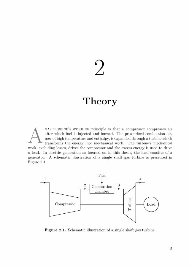
A gas turbine’s working principle is that a compressor compresses airafter which fuel is injected and burned. The pressurized combustion air,now of high temperature and enthalpy, is expanded through a turbine whichtransforms the energy into mechanical work. The turbine’s mechanical

work, excluding losses, drives the compressor and the excess energy is used to drivea load. In electric generation as focused on in this thesis, the load consists of agenerator. A schematic illustration of a single shaft gas turbine is presented inFigure 2.1.

12 3

4Fuel

Compressor

Turbine

Combustionchamber

Load

Figure 2.1. Schematic illustration of a single shaft gas turbine.

5

CHAPTER 2. THEORY

2.1 Twin shaft gas turbinesTwin shaft gas turbines are different, from single shaft machines, in the fact thatthey are running two turbines with mechanically separated shafts. The first one, thecompressor turbine, is as with single shaft gas turbines connected to the compressor.This turbine produces the exact amount of energy the compressor requires, withlosses taken into account. This first part of the twin shaft gas turbine is oftenreferred to as the gas generator. After the gas generator the combustion air is ledto a second turbine, the free power turbine. Here the excess energy is transformedinto mechanical work and used to drive the load through a separate second shaftand possibly a gear box. With no mechanical connection to the compressor, thefree power turbine is independent and is for example able to run at a shaft speedunrelated to other parts of the engine. Due to this the machine type is useful todrive a varied load, the twin shaft gas turbine’s main advantage. Another benefitfrom using separated shafts is, as Cohen et al. [2] describes, that the torque is highat low shaft speeds, a useful property when using a gas turbine for vehicle operation.A schematic illustration of a twin shaft gas turbine is presented in Figure 2.2.

Gas generator

12 3

4 5Fuel

Compressor

Com

pressor

turbine

Combustionchamber

Load

Power

turbine

Figure 2.2. Schematic illustration of a twin shaft gas turbine.

Despite the lack of mechanical coupling between the compressor and power turbine,there is an existing coupling called aerothermal (aero- and thermodynamic) betweenthe two. This means the components are not as independent as can be adopted at firstglance. The phenomenon affects the matching and interaction between componentsand has to be considered in the process of calculating a twin shaft gas turbine.

On multiple shaft gas turbines the power turbine can be differently matched. With aVGV, the power turbine is optimized depending on the prevailing ambient conditions.The SGT-750 can be matched for normal and tropical conditions.

6

2.1. TWIN SHAFT GAS TURBINES

2.1.1 SGT-750

The SGT-750, Figure 2.3, is the company’s latest addition to the product portfolio.Due to its twin shaft configuration and power output of approximately 38MW itis a versatile gas turbine, suitable for numerous applications such as simple cycle,combined cycle and mechanical drive. With DLE technology, NOx emissions arekept below 15ppmv, Siemens AG [3], although emissions remain an issue at partload.

Today emissions at part load are controlled by bleeding pressurized air from afterthe compressor to the gas turbine exhaust. Seen from a performance point of viewthis is the worst possible approach although not to belittle, the easiest and cheapestone. Tageman [4] describes the alternatives and why this inefficient method waschosen in the development process. The bleed method could be made with bleed tothe compressor inlet but problems occurred with mixing the high pressure air withthe ambient. Bypassing air over the burners is a possible solution but was rejecteddue to the can burner setup. Ultimately bleed to the exhaust was chosen due to itssimplicity, robustness and low cost.

Further Tageman [4] describes the way the amount of bleed air is controlled. It isdone by aiming for a target value of T1520 with the load lowered until this target valueis reached. At further lowered load, T1520 is kept constant as a result of graduallyopening the bleed valve allowing pressurized air to be dumped and thus, reducingthe burner mass flow. At a bleed mass fraction exceeding a limit, T1520 is loweredfurther until the lower bound of the temperature, due to emission requirements, isreached.

Figure 2.3. Computer rendered illustration of the SGT-750, Siemens IndustrialTurbomachinery AB [5].

7

CHAPTER 2. THEORY

2.2 General thermodynamicsSome general thermodynamic relations and theory needed to proceed with the theoryof this thesis is presented below.

2.2.1 Cycle efficiency and the ideal Brayton cycle

The ideal cycle for gas turbine engines was invented by George Brayton, hence itis called the ideal Brayton cycle. The thermal efficiency of an ideal Brayton cyclemay be defined in accordance to Çengel and Boles [6, p.471], with notations statedin Table 2.1 and Figure 2.1.

η = Wnet,out

Qin= (h3 − h4)− (h2 − h1)

(h3 − h2) (2.1)

Table 2.1. Notations for the ideal Brayton cycle.

1. Before compression2. After compression3. Before expansion4. After expansion

Assuming constant specific heat capacity the expression is rewritten.

η = (T3 − T4)− (T2 − T1)(T3 − T2) = 1− (T4 − T1)

(T3 − T2) = 1−T1 (T4

T1− 1)

T2 (T3T2− 1)

(2.2)

The thermal efficiency is rewritten as a function of pressure ratio and isentropicexponent using isentropic relations. This is made assuming both the compressionand expansion process to be isentropic and no pressure loss to occur in between, thatis p1 = p4 and p2 = p3.

T2

T1=(p2

p1

) γ−1γ

= πγ−1γ =

(p3

p4

) γ−1γ

= T3

T4(2.3)

η = 1− 1πγ−1γ

= f(π, γ) (2.4)

8

2.2. GENERAL THERMODYNAMICS

2.2.2 Isentropic versus polytropic efficiency

Consider a compression process frompa to pc, according to Figure 2.4. Theisentropic efficiency handles the com-pression as a linear process while in re-ality, a more accurate way to describeit is with the polytropic efficiency asa non-linear polynomial. Calculatinga part process, in example a compres-sion from pa to pb, using the polytropiceffiency will result in the more accurateresult of b′′ instead of b′.

s

T

ap

bpcp

c

a

b ¢¢b¢

Figure 2.4. Comparision of isentropicand polytropic efficiency.

2.2.3 Pipe pressure lossPressure losses due to friction in pipes and ducts are called major losses while theminor losses consists of losses due to specific components, such as valves and bends.The total pressure loss, including both major and minor losses, is defined by theDarcy–Weisbach equation according to Young et al. [7].

∆pfric =(f l

D+∑

KL

)ρ v2

2 (2.5)

The friction loss factor for laminar flows is described by Young et al. [7]. For turbulentflows a dependence of relative roughness, ε/D, is present and the friction loss factorcan be approximated with the Haaland equation according to Haaland [8].

flam = 64Re

(2.6a)

1√fturb

= −1.8 · log10

[(ε/D

3.7

)1.11+ 6.9Re

](2.6b)

Young et al. [7] describes a flow to be laminar if the Reynolds number is belowapproximately 2100 and turbulent if above 4000. Reynolds number is defined asfollows were the velocity is calculated with the mass flow rate in Equation 2.9.

Re = ρ v D

µ(2.7)

9

CHAPTER 2. THEORY

2.3 Performance predictionA gas turbine’s performance at all operating conditions depends on numerous de-scribing parameters, as for example ambient temperature and pressure, rotationalspeed, IGV angle, gas constant etcetera. The large number of parameters can makethe performance difficult to interpret. A way to reduce the number of parametersis to create parameter groups to make the information more perspicuous and alsofacilitate further calculations. In an example Walsh and Fletcher [9] describes a re-duction from eight parameters to three parameter groups. These parameter groupscan be derived using either dimensional analysis, as for example the Buckingham pitheorem, or by creating velocity diagrams based on Mach number. Since the latteris considered easier as well as more often used in the business, it is this method thisthesis will proceed with.

Mach number is defined as a ratio of a velocity and the local speed of sound asin Equation 2.8 according to Çengel and Boles [6, p.780]. Using this, the velocitydiagrams can be expressed based on Mach number as seen in Figure 2.5.

Mav = v√γRT

(2.8)

wc

u

Maw

Mac

Mau

Figure 2.5. Expressing velocity diagram based on Mach number.

To calculate the Mach numbers illustrated in Figure 2.5, Mac, Maw and Mau, amethod of examining the mass flow, rotational speed and pressure ratio described byJonshagen [10] is used.

10

2.3. PERFORMANCE PREDICTION

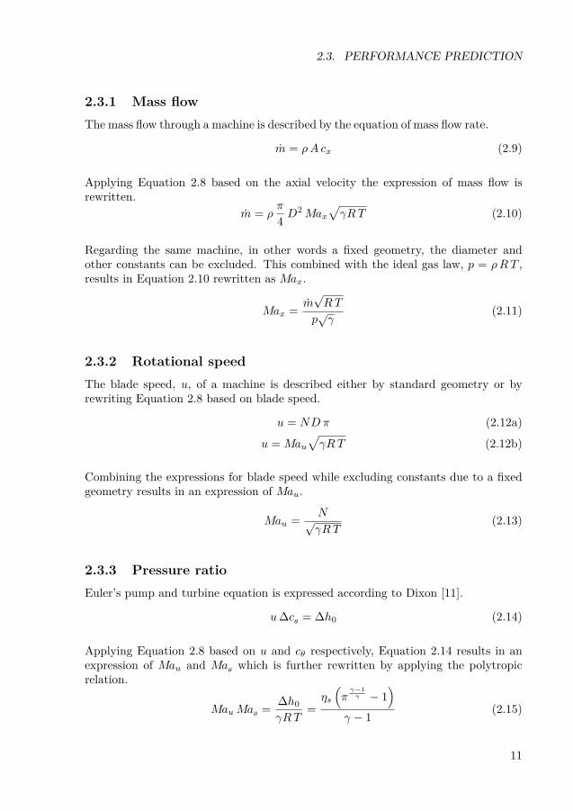
2.3.1 Mass flowThe mass flow through a machine is described by the equation of mass flow rate.

m = ρA cx (2.9)

Applying Equation 2.8 based on the axial velocity the expression of mass flow isrewritten.

m = ρπ

4 D2 Max

√γRT (2.10)

Regarding the same machine, in other words a fixed geometry, the diameter andother constants can be excluded. This combined with the ideal gas law, p = ρRT ,results in Equation 2.10 rewritten as Max.

Max = m√RT

p√γ

(2.11)

2.3.2 Rotational speedThe blade speed, u, of a machine is described either by standard geometry or byrewriting Equation 2.8 based on blade speed.

u = NDπ (2.12a)

u = Mau√γRT (2.12b)

Combining the expressions for blade speed while excluding constants due to a fixedgeometry results in an expression of Mau.

Mau = N√γRT

(2.13)

2.3.3 Pressure ratioEuler’s pump and turbine equation is expressed according to Dixon [11].

u∆cθ = ∆h0 (2.14)

Applying Equation 2.8 based on u and cθ respectively, Equation 2.14 results in anexpression of Mau and Maθ which is further rewritten by applying the polytropicrelation.

MauMaθ = ∆h0

γRT=ηs

(πγ−1γ − 1

)γ − 1 (2.15)

11

CHAPTER 2. THEORY

2.3.4 CharacteristicsUsing the derived Mach numbers, all Mach numbers are known according to Fig-ure 2.6. Consequently, the velocity diagram is resolved. In other words, the gasturbine’s behavior is fully described.

MawMac

Mau

Maθ

Max

Figure 2.6. Velocity diagram based on Mach number.

To clearly visualize the performance of a gas turbine specific component charac-teristics are created. These characteristics, also known as compressor and turbinemaps, are made from plotting the dimensionless parameter groups, that is the derivedMach numbers, to indicate the components performance in all operating conditions.It should be noted that at SIT the pressure ratio itself is used instead of the correctedpressure ratio derived in Equation 2.15. In these maps each point represents a uniquevelocity diagram based on Mach number and thus describes a unique operating case.The maps themselves are also unique for each component and its associated designand reveals the performance of the component in detail. For this reason, the mapsare handled with great confidentiality by the companies in the industry.

Schematic illustrations of compressor and turbine maps are presented in Figure 2.7and 2.8. In the compressor map the surge line is marked. An operating point abovethis line means the flow is unstable and can separate due to high positive incidenceaccording to Razak [12]. This can in turn lead to an abrupt reversal of the flowthrough the compressor, potentially damaging the components. To assure a stablecompression a surge margin is introduced. This safety margin defines the distancebetween the operating point and the surge line. To illustrate a machines operatingrange a running line is commonly introduced. This is a line connecting all steady stateoperating points at certain conditions. Additional information typically presentedin compressor maps are lines of constant corrected speed and islands representingconstant isentropic efficiency.

12

2.3. PERFORMANCE PREDICTION

π

γp

RTmMa

x

0

0

0RT

NMa

u

Islands of constant

isentropic efficiency Surge line

Running line

Figure 2.7. Schematic illustration of a compressor map.

Regarding turbine maps a difference is made between the cases if choking occurs inthe stator or the first rotor. Noticeable about turbine maps is that the flow capacityis constant, in other words the flow is choked, throughout a wide range of pressureratio.

0

0

p

RTmMa

x

0RT

NMa

u

(a)

0

0

p

RTmMa

x

0RT

NMa

u

(b)

Figure 2.8. Schematic illustrations of turbine maps where choke occurs in the stator(a) or in the first rotor (b).

13

CHAPTER 2. THEORY

2.3.5 Corrected parameters

A machine’s performance while running at ambient conditions deviating from ISOconditions is hard to interpret. To make it possible to compare a machine’s perfor-mance regardless of its running conditions so called corrected or referred parametersare formed to reduce the number of depending variables further. This is done bycorrecting the parameters with reference values of certain variables as for exempleγ and R. The corrected parameters most often used in compressor calculations arecorrected shaft speed and mass flow.

Ncorr√γrefRrefTref

= N√γRT

⇔ Ncorr = N√γ

γrefR

RrefTTref

(2.16a)

mcorr

√Tref

pref

√Rrefγref

= m√T

p

√R

γ⇔ mcorr =

m√

TTrefp

pref

√γrefγ

R

Rref(2.16b)

Having a reference temperature for a turbine is inconvenient as the full load TIT mayvary due to fuel specification and differs for different versions of the machine. Thecorrected parameters however can be formed in any manner, what matters is thatthe method is consistent throughout the calculation process. Examples of customparameters used at SIT are aero speed and flow capacity. These are variations ofthe corrected shaft speed and mass flow in Equation 2.16a and 2.16b respectively.It should be noted that these parameters are based on the inlet values before thecooling air is mixed into the flow, in example TIT is T1500 and not T1520.

AScorr = N√γ

γrefR

RrefT

(2.17a)

CTcorr = m√T

p

√γrefγ

R

Rref(2.17b)

14

2.4. EXHAUST GAS RECIRCULATION

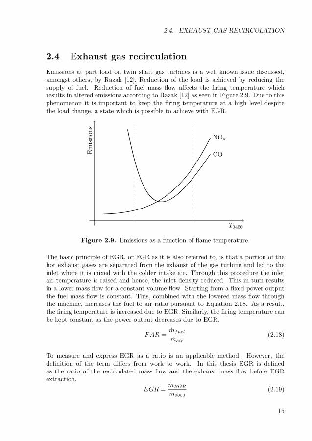
2.4 Exhaust gas recirculationEmissions at part load on twin shaft gas turbines is a well known issue discussed,amongst others, by Razak [12]. Reduction of the load is achieved by reducing thesupply of fuel. Reduction of fuel mass flow affects the firing temperature whichresults in altered emissions according to Razak [12] as seen in Figure 2.9. Due to thisphenomenon it is important to keep the firing temperature at a high level despitethe load change, a state which is possible to achieve with EGR.

T3450

Emiss

ions

CO

NOx

Figure 2.9. Emissions as a function of flame temperature.

The basic principle of EGR, or FGR as it is also referred to, is that a portion of thehot exhaust gases are separated from the exhaust of the gas turbine and led to theinlet where it is mixed with the colder intake air. Through this procedure the inletair temperature is raised and hence, the inlet density reduced. This in turn resultsin a lower mass flow for a constant volume flow. Starting from a fixed power outputthe fuel mass flow is constant. This, combined with the lowered mass flow throughthe machine, increases the fuel to air ratio pursuant to Equation 2.18. As a result,the firing temperature is increased due to EGR. Similarly, the firing temperature canbe kept constant as the power output decreases due to EGR.

FAR = mfuel

mair(2.18)

To measure and express EGR as a ratio is an applicable method. However, thedefinition of the term differs from work to work. In this thesis EGR is definedas the ratio of the recirculated mass flow and the exhaust mass flow before EGRextraction.

EGR = mEGR

m0850(2.19)

15

CHAPTER 2. THEORY

2.4.1 Additional positive effects of EGR

Aside from keeping the firing temperature high with lowered load, the purpose ofEGR in this thesis, the method also offers several other benefits. If the hot exhaustgases are mixed with the intake air before the intake air filter, the hot recirculationworks as a free anti icing system. Thus, a separate system to deal with icing of theintake air filter will not be needed, a system that would increase losses.

Another advantage of implementing EGR in the gas turbine cycle is that the concen-tration of CO2 is increased. This in turn significantly decreases the energy demandof CCS as shown by Li et al. [13].

2.4.2 Limitations of EGR

Temperature limitationsTo reduce weight, and also simplify the manufacturing process and hence the costs,the inlet casing of the SGT-750 is made of a composite material, Tageman [4]. Nilsson[14] establishes that with the material used today, this implies a temperature limit of90 ◦C at continuous load while a higher temperature, 130 ◦C, is allowed instantaneous.Since the purpose of EGR is to increase the inlet temperature, this is an unquestion-able limitation. However, in the case of an inlet temperature rise above an acceptablelevel other composite materials such as Vinyl Ester can be used, Nilsson [14]. In thiscase the temperature limit increases to approximately 160 – 200 ◦C.

An increase in compressor inlet temperature also results in a temperature rise furtherdown the compressor. Eventually a temperature is reached when the flow is to hot towork as necessary cooling flow. The problem is examined by Andersson [15], resultingin a limit in the compressor outlet temperature.

The positive side effect of an EGR system that works as a free anti icing system alsohas its limitations. Jonsson [16] states that todays solution of handling ventilationto the SGT-750 enclosure is to use the same intake air filter as to the machine itself.This problem is however easy to solve with a rather simple construction modification.Furthermore, the intake filter itself is limited in temperature, according to Jonsson[16] at 80 ◦C locally for hot strings if the flow is inhomogeneously mixed and at 70 ◦Cin general. A possible solution to this problem is to mix the hot exhaust gases withthe intake air after the filter, but the advantage of a free anti icing system is thenlost. Also, this solution would have a negative impact on the efforts to achieve anas clean as possible environment after the intake air filter. This effort is, accordingto Tageman [4], made to minimize the risk of getting unwanted items, such as metalobjects, in the system that may be harmful to the compressor.

16

2.4. EXHAUST GAS RECIRCULATION

Oxygen limitationsWith increasing EGR the oxygen content is decreasing in the combustion chamberoutlet. A lack of oxygen results in incomplete combustion, an undesirable state,which limits the percentage of EGR possible to fulfill. According to Janczewski [17]a minimum oxygen content of 8% in the combustion chamber outlet is required toensure complete combustion.

LifingLifing of gas turbines are greatly related to rotational speed since centrifugal tensilestress of the blades relates to rotational speed according to Equation 2.20, Cohen etal. [2, p.298]. This implies that possible variations in rotational speed due to variationin load are important. There is a limit of 9400 rpm for the SGT-750, according toTageman [4]. However, it should be borne in mind that an increased speed alwaysimplicates a decrease in lifetime of a gas turbine.

σ ∝ AN2 (2.20)

Further example of a factor affecting the lifing of gas turbines is the TIT. A highertemperature results in a shortage of lifespan for the machine according to Jonshagen[18].

2.4.3 Practical aspects of implementing EGR

When implementing EGR in the gas turbine cycle some practical aspects has to betaken into account. The flow has to be extracted from the exhaust at a convenientlocation. It has to be led through piping of sufficient dimensions and be pressurizedby a fan. This fan can also, in some cases, serve as a component to mix the intakeair with the hot exhaust gases to guarantee a good temperature distribution of theflow. Finally the flow has to be inserted back into the cycle.

17

CHAPTER 2. THEORY

2.5 IPSEpro and the Newton-Raphson methodIPSEpro, a software developed by SimTech Simulation Technology, is a heat andmass balance calculation program. It is a matrix solver that puts all equations ofa system in a matrix. To speed up the calculating process, the program at firstdivides the matrix into sub matrixes to separate non depending variables from eachother. After this, the equations in each submatrix are solved simultaneously withthe Newton-Raphson method.

2.5.1 IPSEpro

The working principle of IPSEpro is that the model built is composed of componentscontaining the heat and mass balance equations necessary for equilibrium. The com-ponents and its equations are accessible in the complementary software MDK. MDKis a software used to view and modify existing equations, but also to add variablesand equations into existing components or creating brand new components. MDKstores the components in so-called library files. With the software SimTech providesa standard library of power plant components called advanced power plant library orapplib.

In IPSEpro the tolerances and iteration parameters are set in the software settings.These settings works as criteria for convergence of the calculations. To carry outa full calculation, the correct number of parameters in relation to the number ofexisting equations in MDK also has to be set. The software then solves the equationsystem according to the Newthon-Raphson method.

2.5.2 The Newton-Raphson method

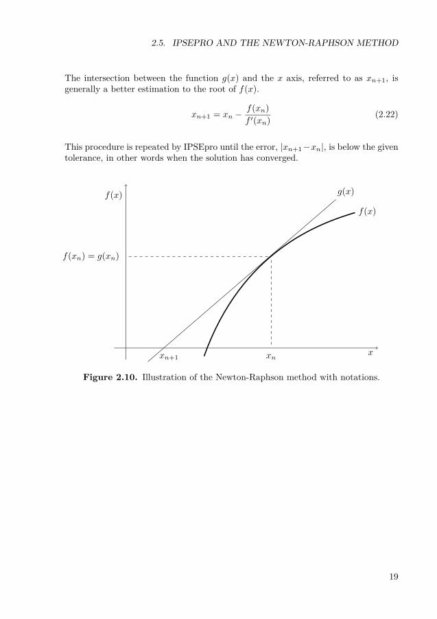
The basic principle of the Newton-Raphson method is that it, on the basis of astarting estimate, finds better and better approximations to the roots of a functionon the form of f(x) = 0. As the iteration continues the approximations convergesand a solution is obtained. This method is a fast way to solve a large number ofequations although it lacks in reliability because of the risk of calculating the wrongor no roots with poor initial estimates. The method can mathematically be describedas follows, with notations according to Figure 2.10.

By starting with the estimate xn, f(xn) is calculated and f(x) is estimated locallywith its linear tangent g(x) given by the point slope formula described by Böiers andPersson [19, p.25].

g(x) = f ′(xn)(x− xn) + f(xn) (2.21)

18

2.5. IPSEPRO AND THE NEWTON-RAPHSON METHOD

The intersection between the function g(x) and the x axis, referred to as xn+1, isgenerally a better estimation to the root of f(x).

xn+1 = xn −f(xn)f ′(xn) (2.22)

This procedure is repeated by IPSEpro until the error, |xn+1−xn|, is below the giventolerance, in other words when the solution has converged.

x

f(x)

f(x)

xn+1 xn

f(xn) = g(xn)

g(x)

Figure 2.10. Illustration of the Newton-Raphson method with notations.

19

3Methodology

T he general approach to fulfill the purpose of this thesis was to create astandard model of the gas turbines examined. The model was constructedto automatically read Siemens component characteristics to ensure its va-lidity. Furthermore, the model was validated against Siemens performance

programs to ensure its correspondence with reality. A model that was consistentwith the performance programs was able to give a useful indication of how the gasturbine would behave under changing circumstances. The model was thereafter com-plemented with EGR and its impact and potential was examined as a method toimprove the gas turbine’s performance and emissions at part load.

3.1 Software selectionThe software used in the work process were naturally selected. IPSEpro was selectedto create the model since it is the standard software to perform model calculations atSIT’s department of research and development. Due to the same reason, the programselected to validate the model’s calculations was the SIT intern performance calcu-lation program, GTPerform. The work with developing a DLL file was conductedin Microsoft Visual Studio 2010, with C++ as programming language. This choicewas made mainly because earlier work of creating executive files, with the purpose ofmaking IPSEpro communicate with text files, using this software and language hasbeen carried out at the Department of Energy Sciences by Mondejar [20].

21

CHAPTER 3. METHODOLOGY

3.2 Development of DLL fileTo get IPSEpro to load data from Siemens text files of component characteristics, aDLL file was developed. DLL files provides a way for an application to call functionsthat are not part of its executable code and are the recommended files to implementexternal functions in MDK according to SimTech [21]. The technicalities and methodbehind creating the file is described by Mondejar [20]. A disadvantage of using DLLfiles to communicate with IPSEpro is that error messages occurring when executingthe file are difficult to handle. The option of passing error messages from the DLLfile to IPSEpro is available in MDK but its applicability is limited.

3.2.1 Read data

A function read was written to read the data from the text files. The purpose of thefunction was to read and interpret the information from Siemens component charac-teristics and store it in variables. The main technical challenge of the read functionwas to make the DLL file future-proof and versatile. In example, the characters of astring was not read from character x to y on a given line but instead read from thefirst character not consisting of a white space to the character before next occurringwhite space.

3.2.2 Perform calculations

The calc function was written to perform the calculations. It calculates the massflow and efficiency based on the input data of corrected shaft speed and pressureratio by interpolating in the characteristics. Specific parameters were built in thecalculations to control whether the input parameters were within the boundaries ofthe characteristics. If not, the calculations returned excessive results to IPSEproto force a change in derivative and thus, a changed input in the next iteration ofcalculations.

3.2.3 Main functions and derivatives

The necessary functions to get the DLL file to interact with IPSEpro were created.These consisted of one main function and two derivatives for each return value. Thederivatives were numerically calculated using the definition of the derivative accordingto Böiers and Persson [19, p.187].

f ′(x) = limx→ 0

f(x+ h)− f(x)h

(3.1)

22

3.2. DEVELOPMENT OF DLL FILE

3.2.4 Description of the code

An extract of the actual code written, the preamble and functions related to thecompressor, is presented in the Appendix A whereas a more general description ofthe code’s cornerstones is presented in sequential order below.

• Initially some basic libraries are included.

• The necessary functions for a DLL file to communicate with IPSEpro are includedaccording to the manual by Mondejar [20].

• Some miscellaneous objects as vectors and other variables are defined.

• The function read:– After the input data file is opened a while loop traverses and reads all the lines

of the file.– After commentary lines are skipped some miscellaneous values as for example

the number of IGV angles and number of speed lines are read.– The code continues with looping all speed lines and for each speed line traversing

and reading its included lines of values. In the case of the compressor thesevalues are the corrected mass flow, pressure ratio and polytropic efficiency whilethey for the turbines are flow capacity, pressure ratio and isentropic efficiency.

– The input data file is closed.

• The function calc:– The speed lines are traversed to find the two speed lines relevant to interpolate

between with regard to the input data of speed.– For each of the two speed lines, its corresponding table of pressure ratio is

traversed to find the two pressure ratios relevant to interpolate between withregard to the input data of pressure ratio.

– With linear interpolation the return values are calculated. These are mass flowand polytropic efficiency for the compressor and flow capacity and isentropicefficiency for the turbines. If the input data is outside of the characteristics,the function returns a mass flow or flow capacity of zero and an efficiency of100% to force IPSEpro to change its derivatives, as described in Section 3.2.2.

– In the case of the power turbine an extra input data of turbine match is usedto determine which characteristics to use.

• External functions and associated derivatives are included.

23


3.3 Construction of modelInitially a model was put together using standard components from applib. Theworking procedure was to start from a basic model of a gas turbine and complementit with more advanced components as the work progressed. This resulted in a newlibrary containing all modified components and equations. Throughout the process,the work was performed with a general mindset to make the model durable andincrease its interchangeability for future possible changes of the gas turbine configu-ration.

The SIT specific theory and nomenclature used in the process of modeling the com-ponents is described in the SIT Performance Model by Sjödin [22].

3.3.1 SAS

Construction of the secondary air system started with examining the gas turbine’sreference file. This file states from where and at what temperature and enthalpyratio in the compressor the cooling flows are extracted, and at what location in theprocess they are inserted again. With this information the necessary splitters andmixers could be modeled.

The biggest effort put into this part of modeling was with creating the necessarysplitters for the cooling flows, Figure 3.1a. To facilitate future development of modelsof other gas turbines in the company, they were made general. Every splitter wascreated with three, and in some cases four, output ports. When adding the splitterto the model, every port’s destination was selected in a drop down list as presentedin Figure 3.1b, for example 0850, leak or no connection. These choices made thecorrect splitter fraction to be obtained from the global object containing all fractionsfrom the gas turbine reference file.

(a) Cooling flow splitter. (b) Port settings.

Figure 3.1. Secondary air system splitter with settings.

24

3.3. CONSTRUCTION OF MODEL

3.3.2 Modeling with characteristicsThe characteristics describes, as mentioned in Section 2.3.4, a components perfor-mance and behavior in all operating conditions. The general approach when modelingwith characteristics is to set a reference point to which all other parameters can berelated. In this case it was done by setting the reference values as input data in thecomponents in IPSEpro.

The relation between the actual, relative and reference values of a variable was cal-culated as follows. However, the pressure ratio was calculated differently to ensure apressure ratio of one when no pressure rise or drop occurs, in accordance with Sjödin[22].

Xrel = X

Xref(3.2a)

πrel = π − 1πref − 1 (3.2b)

3.3.3 CompressorWith set reference values, the corrected parameters were calculated according toEquation 2.16a and 2.16b and with Equation 3.2a and 3.2b, the relative parameterswere calculated. After this, functions were created in MDK to communicate withthe DLL file and calculate the mass flow and polytropic efficiency as a function ofrelative speed and pressure ratio.

mrel = f(Nrel, πrel) (3.3a)ηp,rel = f(Nrel, πrel) (3.3b)

3.3.4 TurbineA problem regarding the turbine expansion is that it either has to start from the realturbine inlet, in the example of the compressor turbine at 1500, or from a fictitiousstate where all cooling air is mixed in with the flow, at 1520. Neither of the methodsare correct since it, in reality, is a gradual process. This was solved by modelingthe expansion from the fictitious mixed inlet state and placing probes in the modelbefore the cooling air was mixed in. These probes were used to communicate thevariable values at the location of the probe with the turbine to calculate the differentparameters. This was done because if all variables used to calculate the parametersfor the characteristics, for example flow capacity, were fetched at the mixed inlet, achange in cooling mass flow would not affect these parameters.

The corrected parameters were calculated according to Equation 2.17a and 2.17b,after which the relation between the corrected, relative and reference value of vari-

25


ables in the turbine were calculated with Equation 3.2a and 3.2b. Functions werecreated to calculate flow capacity and isentropic efficiency as a function of correctedaero speed, pressure ratio and matching conditions, using the DLL file created. Thematching condition indicated whether the function should perform calculations us-ing normal or tropical matching of the gas turbine. This option was however onlyrelevant for the power turbine.

CTrel = f(ASrel, πrel,match) (3.4a)

ηs,rel = f(ASrel, πrel,match) (3.4b)

3.3.5 Combined cycle

An additional model was created were the gas turbine, referred to as the top cyclein a combined cycle, was added an existing model of a bottoming cycle from SIT.An existing model was used since modeling this was not considered a purpose ofthis thesis. The bottoming cycle consisted of a dual pressure heat recovery steamgenerator, HRSG, using heat from the exhaust gases of the gas turbine to producesteam for a simple Rankine steam cycle.

26

3.4. VALIDATION

3.4 ValidationThe model’s conformance with Siemens performance programs was a key criterion forthe work to proceed. A number of important sections throughout the machine wasexamined and key values in these sections were compared against the correspondingvalues calculated by GTPerform. This process was performed for different operatingconditions with varied ambient temperature and load. Sections were the deviationwas significant were examined thoroughly in MDK and errors were corrected.

With the goal to eliminate the residual error, the main components were examinedseparately. With values from GTPerform set in IPSEpro as input and output datain the components, their calculations were verified. The results yielded a remainingerror of the same magnitude resulting in further investigation. A single stream withthe same composition, temperature and pressure as in GTPerform was examined.With a remaining error the reason was found to be a difference in gas data, thephysical properties are calculated differently. IPSEpro uses JANAF, Joint ArmyNavy Air Force, Thermochemical Tables [23] whereas GTPerform uses NASA SP-273. The deviation was considered to be within the margin of error and the processof model validation was completed.

An issue appearing during the process of validating the compressor component sep-arately was that the input data to the DLL file sometimes was outside the tables ofcharacteristics. The interpolation in the function calc would not work and the modeldid not converge, it was instable. An idea if creating so called beta lines, slantinglines in the compressor map as input data was examined but the issue was solvedautomatically when connecting the compressor to the compressor turbine. The gasgenerator as a unit affected the quantities simultaneously and the model becamestable, the running line basically worked as a beta line.

27


3.5 Complementing with EGRThe model was complemented with EGR in different setups depending on whetherit was for the simple or combined cycle.

3.5.1 Simple cycle

In the case of the simple cycle, the model was complemented with a stream recir-culating exhaust gases from the exhaust before the outlet pressure drop, at 0850, tothe inlet before the intake air filter, at 0100. To drive the flow forward and managethe issue of mixing the cold inlet air and hot exhaust gases to guarantee a goodtemperature distribution, a fan was added to the model. This fan was powered witha motor affecting the total power produced since the motor consumes power.

The performance of the fan was set to necessary values according to Andersson [24]with a total pressure rise of 13.26mbar over the complete section of EGR. In additionthe isentropic, electrical and mechanical efficiencies of the motor were all set to 90%.This was made to ensure a satisfying safety margin in the calculations although boththe electrical and mechanical efficiency might be too restrictively set. To satisfythe demands of the fan, a maximal inlet temperature of 300 ◦C had to be guaranteedaccording to Tageman [4]. This was ensured by mixing a sufficient part of the ambientair with the recirculated exhaust gases before the fan.

3.5.2 Combined cycle

A stream recirculating the exhaust gases from after the HRSG to the gas turbineinlet before the intake air filter, at 0100, was added. To simulate the pressure drop ofthe HRSG, the outlet pressure drop was approximated to 25mbar. A fan and motor,as used in the simple cycle, was necessary also in this case. However, mixing therecirculated exhaust gases with the intake air before this fan was not necessary dueto the lower temperature of the gases. In addition to this, the feed water pumps inthe bottoming cycle were added motors with the same specifications as the EGR fanconsuming power and hence, negatively impacting the total power produced.

A variant of the combined cycle was also created with the same EGR case as forthe simple cycle to be able to fully compare the two and clarify the potential of thecombined cycle.

28

3.6. ANALYSIS

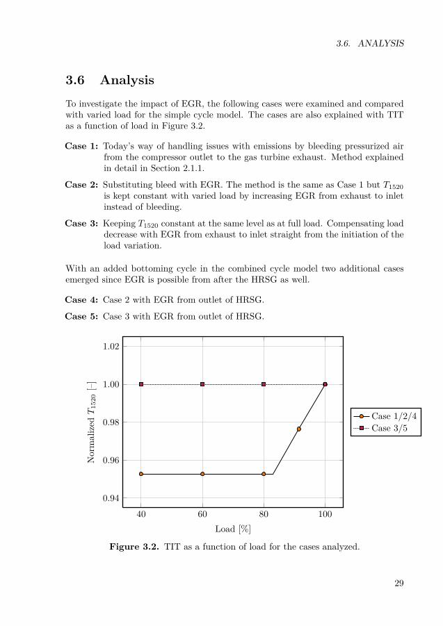
3.6 AnalysisTo investigate the impact of EGR, the following cases were examined and comparedwith varied load for the simple cycle model. The cases are also explained with TITas a function of load in Figure 3.2.

Case 1: Today’s way of handling issues with emissions by bleeding pressurized airfrom the compressor outlet to the gas turbine exhaust. Method explainedin detail in Section 2.1.1.

Case 2: Substituting bleed with EGR. The method is the same as Case 1 but T1520is kept constant with varied load by increasing EGR from exhaust to inletinstead of bleeding.

Case 3: Keeping T1520 constant at the same level as at full load. Compensating loaddecrease with EGR from exhaust to inlet straight from the initiation of theload variation.

With an added bottoming cycle in the combined cycle model two additional casesemerged since EGR is possible from after the HRSG as well.

Case 4: Case 2 with EGR from outlet of HRSG.

Case 5: Case 3 with EGR from outlet of HRSG.

40 60 80 100

0.94

0.96

0.98

1.00

1.02

Load [%]

Normalized

T15

20[–]

Case 1/2/4Case 3/5

Figure 3.2. TIT as a function of load for the cases analyzed.

29


3.6.1 Comparision

All cases were examined with ambient temperature of 15 ◦C and normal turbinematch of the power turbine as well as with ambient temperature of 30 ◦C and tropi-cal turbine match. Significant parameters were plotted against load or other key pa-rameters to illustrate the gas turbine’s performance and behavior at part load. Thedifferences between the cases were then analyzed based on the theory and results.Further tests were performed to either eliminate or determine certain parameter’sinfluence on the results.

The cases were examined with decreasing load from 100% to 40%. In the caseswith EGR from the HRSG outlet, Case 4 and 5, the combustion turned problematicwith decreasing oxygen content due to increasing EGR. The requirement of oxygencontent in the combustion chamber outlet was not satisfied at lower loads and thecalculations could not be performed all the way down to 40%.

To make the comparison fair and make the cases similar T1520 was allowed to bereduced to the same level in Case 1, 2 and 4. As mentioned in Section 2.1.1, inthe case of bleeding, T1520 is allowed to be lowered further after a specific bleedmass fraction is reached. This would have had a positive effect on the performancewhile affecting emissions negatively and allowing it in the comparison would be likecomparing apples and oranges and was therefore considered irrelevant.

It should be borne in mind throughout the analysis that the SGT-750 is not actuallydesigned and optimized to work in a combined cycle. The exhaust gas temperatureat ISO conditions is relatively low, 459 ◦C [3], resulting in poor performance of thebottoming cycle.

3.6.2 Practical analysis

The practical implementation of EGR was analyzed by calculating the needed diam-eter of the pipes to satisfy different pressure losses with the equations described inSection 2.2.3. This was done using goal seek, a numeric approximation method. Byiteration different diameters were used to try to satisfy given pressure losses, in thiscase a pressure loss of 13.26mbar in accordance with Andersson [24] and 0.1 bar asan arbitrary estimate. The lower of these losses was chosen because the calculationsthroughout this thesis are based on this pressure loss as described in Section 3.5.1while the latter was examined because a higher accepted pressure loss would resultin a reduced diameter.

The assumptions made for the pipe loss calculations are presented below. The valuesare assumed with conditions after the EGR fan since it is physically located close tothe extraction point and most of the recirculation actually occurs after this fan.

30

3.6. ANALYSIS

• The pipe length is assumed to be 10m for the simple cycle and 15m for thecombined cycle since the distance is further in this case.

• Equivalent roughness is approximated as the roughness for commercial steel, 0.045mm[7, table 8.1].

• The dynamic viscosity of air at 300 ◦C is used, 2.98·10−5 Pa s [7, table B.4]. This issince the combustion is made with excess oxygen resulting in nitrogen gas as thedominant element of the flue gases as is the case with ambient air. The dynamicviscosity is independent of pressure.

• For the simple cycle the mass flow and density at 50% load are used while for thecombined cycle the values related to an oxygen content of 8%, resulting in a loadof 62.134%, are used.

• The loss coefficient was estimated with four long radius 90° flanged bends and onegate valve ¼ closed resulting in a total loss coefficient of 1.06.

As the greater of the two pressure drops examined would have had negative influenceon the performance, the power consumed by the fan and the cycle efficiency were cal-culated to assure a change within the limits of what is considered acceptable.

The material needed for a safe recirculation was determined to be 16Mo3 in collabo-ration with Lindman [25] with reference to a conducted project regarding anti icingpiping. This steel is, according to one supplier, able to withstand wall temperaturesof approximately 530 ◦C [26].

31

4Results

T he standard model of the SGT-750 created in IPSEpro as a part of thisthesis is based on the gas turbine’s characteristics which cannot be madepublic. However, an illustration of the model is presented in Figure 4.1.The process also resulted in models with EGR instead of bleed, used for

further work in this thesis. All models are relatively general in their execution andtherefore future proof for further work and development. This will also facilitate anyadjustments to construct models in IPSEpro of other gas turbines in the company’sproduct portfolio.

G19

Inlet

G11

G12

G13

Diffuser

SGT-750.pro (Default) 02/18/15 07:47:24

Figure 4.1. Standard model of the SGT-750 with bleed.

33

CHAPTER 4. RESULTS

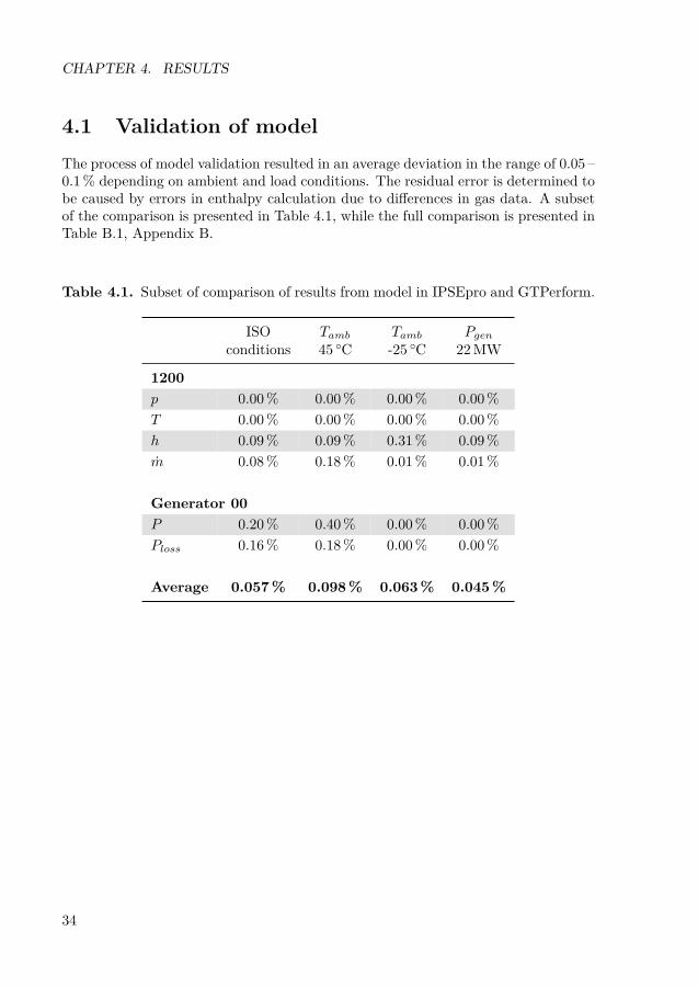
4.1 Validation of modelThe process of model validation resulted in an average deviation in the range of 0.05 –0.1% depending on ambient and load conditions. The residual error is determined tobe caused by errors in enthalpy calculation due to differences in gas data. A subsetof the comparison is presented in Table 4.1, while the full comparison is presented inTable B.1, Appendix B.

Table 4.1. Subset of comparison of results from model in IPSEpro and GTPerform.

ISO Tamb Tamb Pgenconditions 45 ◦C -25 ◦C 22MW

1200p 0.00% 0.00% 0.00% 0.00%T 0.00% 0.00% 0.00% 0.00%h 0.09% 0.09% 0.31% 0.09%m 0.08% 0.18% 0.01% 0.01%

Generator 00P 0.20% 0.40% 0.00% 0.00%Ploss 0.16% 0.18% 0.00% 0.00%

Average 0.057% 0.098% 0.063% 0.045%

34

4.2. SIMPLE CYCLE

4.2 Simple cycleThe result of comparing the three cases studied will be presented through plottingand examining relevant parameters’ variation with load. As mentioned in Section 3.6,Case 1 is using bleed, Case 2 is lowering the mixed TIT to the same level as withbleed while in Case 3 it is kept high throughout the load variation. It should benoted that some results are normalized due to confidentiality.

4.2.1 EGR

The percentage of recirculated mass flow, the definition of EGR in this thesis, isincreasing with lowered load. An in principle linear behavior is seen when examiningEGR as a function of load resulting in a recirculation with ISO conditions and normalmatch in the range of 7 – 9% on 50% load depending on the case studied as seen inFigure 4.2. The same overall behavior is found when the gas turbine is tropicallymatched.

40 50 60 70 80 90 100

0

2

4

6

8

10

12

Load [%]

EGR

[%]

Case 1Case 2Case 3

Figure 4.2. EGR as a function of load for normal match.

35

CHAPTER 4. RESULTS

4.2.2 Cycle efficiency and pressure ratio

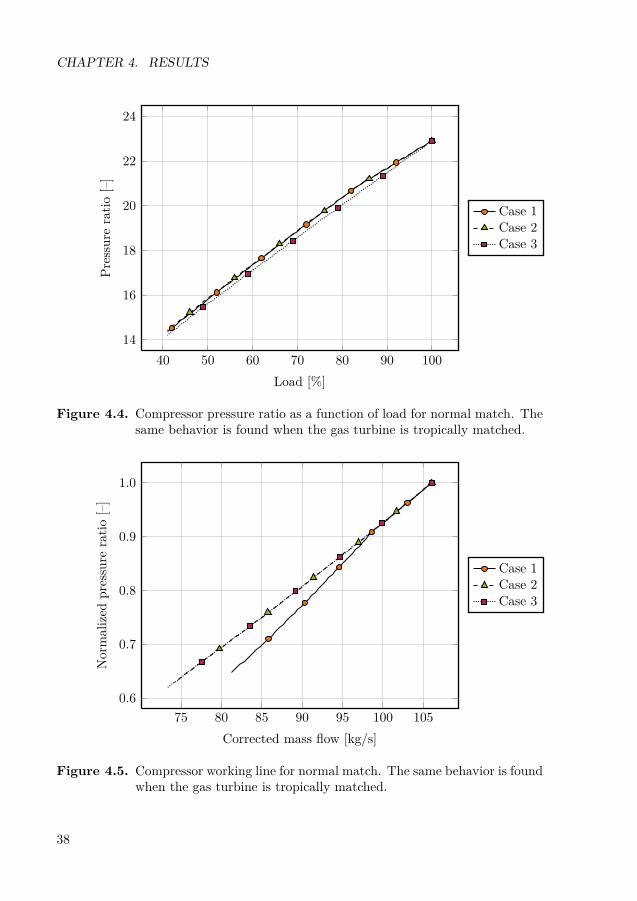
It is found that the cycle efficiency increases significantly with EGR in relation tobleed as presented in Figure 4.3. The reason is that when bleeding, a noticeableportion of pressurized air is dumped to the exhaust. Air that has been added work bythe compressor but is not utilized in the process. A difference in cycle efficiency is alsoobserved in the comparison between the different cases of EGR, Case 2 and 3. Thisrelates to the difference in pressure ratio presented in Figure 4.4 since Equation 2.4states that efficiency is a function of pressure ratio.

In Figure 4.4 a difference in pressure ratio cannot be spotted between Case 1 and 2although the data yields a minor deviation. The cases differs slightly in heat inputdue to the difference in cycle efficiency. This small difference multiplied with a fuelto air ratio in the range of two percent results in a basically equal pressure ratio inthe two cases.

The pressure ratio is also examined and presented as a compressor working line inFigure 4.5. It reveals a running line in Case 2 and 3 closer to the surge line than inCase 1. Despite the fact that the cases of EGR results in a higher efficiency, problemsregarding stability must be considered. When running a gas turbine, a safety marginto surge is necessary to manage changing conditions as for example rapid load rampup. That being said, these results does not disclose the surge margin.

36

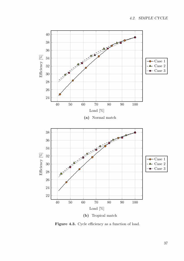
4.2. SIMPLE CYCLE

40 50 60 70 80 90 100

24

26

28

30

32

34

36

38

40

Load [%]

Efficien

cy[%

]

Case 1Case 2Case 3

(a) Normal match

40 50 60 70 80 90 100

22

24

26

28

30

32

34

36

38

Load [%]

Efficien

cy[%

]

Case 1Case 2Case 3

(b) Tropical match

Figure 4.3. Cycle efficiency as a function of load.

37

CHAPTER 4. RESULTS

40 50 60 70 80 90 10014

16

18

20

22

24

Load [%]

Pressure

ratio

[–]

Case 1Case 2Case 3

Figure 4.4. Compressor pressure ratio as a function of load for normal match. Thesame behavior is found when the gas turbine is tropically matched.

75 80 85 90 95 100 1050.6

0.7

0.8

0.9

1.0

Corrected mass flow [kg/s]

Normalized

pressure

ratio

[–]

Case 1Case 2Case 3

Figure 4.5. Compressor working line for normal match. The same behavior is foundwhen the gas turbine is tropically matched.

38

4.2. SIMPLE CYCLE

4.2.3 Component efficiencies

The compressor polytropic efficiency varies only slightly between the three casesstudied, as seen in Figure 4.6. The increased compressor inlet temperature leads toan operating point further from the design point and hence, a decrease in compressorefficiency.

To illustrate that the overall results are only vaguely related to the component eff-iciencies, the compressor polytropic efficiency, with reference to Section 2.2.2, was setconstant which revealed close to no change in cycle efficiency. The turbine efficienciesdoes not either vary appreciably. In conclusion, the variation in component efficien-cies due to EGR is found to have very little influence on the overall cycle.

40 50 60 70 80 90 1000.975

0.980

0.985

0.990

0.995

1.000

Load [%]

Normalized

polytrop

iceffi

cien

cy[–]

Case 1Case 2Case 3

Figure 4.6. Compressor polytropic efficiency as a function of load for normal match.The same behavior is found when the gas turbine is tropically matched.

39

CHAPTER 4. RESULTS

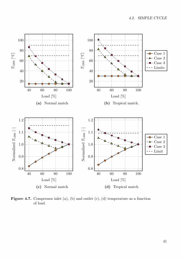
4.2.4 Compressor temperatures

The compressor temperatures varies with load according to Figure 4.7. The limit ofcompressor inlet temperature at 90 ◦C is reached in Case 3 with tropical matching ofthe power turbine. As mentioned in Section 2.4.2 this limit is not set in stone andthe compressor inlet can handle higher temperatures momentarily. That being said,the temperature limit in the compressor outlet is also reached in this case.

Furthermore, if the EGR is used as an anti icing system and the hot exhaust gasesare mixed with the ambient air before the intake air filter the general temperaturelimit of 70 ◦C applies. However, there is a workaround of this problem as discussedin Section 2.4.2 of not using EGR as an anti icing system.

4.2.5 Shaft speed

The physical rotational speed is an important parameter in aspects of solid mechanicsand lifing. The results presented in Figure 4.8a and 4.8b yield that with increasingrate of EGR due to lowered load the physical shaft speed increases, while it decreaseswith bleed. The behavior of Case 2 is especially noticed to at first decrease in shaftspeed then, when EGR is initiated, increase again. The downward trend of shaftspeed due to bleed can be explained by a lower mass flow through the turbine. Thisresults in a decrease in pressure due to a relatively constant flow capacity according toEquation 2.17b. A lower pressure build-up in turn leads to lower shaft speed.

The upward trend of shaft speed due to EGR is a consequence of the fact that morework has to be performed to compress the heated inlet air. The compressor com-pensates this with an increase in mass flow, in other words an increased shaft speed.Worth noticing is that in Case 3 the rotational speed limit of 9400 rpm is reached atapproximately 60% load and tropical match, a limit not acceptable to exceed. Also,studying the corrected compressor speed in Figure 4.8c and 4.8d reveals a decreasein all shaft speeds when corrected for temperature and gas properties.

While physical shaft speed is of importance in terms of mechanical aspects, theturbine aero speed is the parameter perceived by the flow affecting the aerodynamicperformance in general. The aero speeds presented in Figure 4.9a and 4.9b shows anincrease in all cases except for Case 1 after the bleed valve is opened. When bleedis initiated a rapid change occurs and the aero speed is decreasing. This behavior isconsistent and impacts for example the cycle efficiency as seen in Figure 4.3 where asudden change in gradient for Case 1 is found at just over 80 percent load.

40

4.2. SIMPLE CYCLE

40 60 80 100

20

40

60

80

100

Load [%]

T12

00[◦C]

(a) Normal match

40 60 80 100

20

40

60

80

100

Load [%]

T12

00[◦C] Case 1

Case 2Case 3Limits

(b) Tropical match.

40 60 80 1000.8

0.9

1.0

1.1

1.2

Load [%]

Normalized

T13

00[–]

(c) Normal match

40 60 80 1000.8

0.9

1.0

1.1

1.2

Load [%]

Normalized

T13

00[–]

Case 1Case 2Case 3Limit

(d) Tropical match

Figure 4.7. Compressor inlet (a), (b) and outlet (c), (d) temperature as a functionof load.

41

CHAPTER 4. RESULTS

40 60 80 1008.4’

8.6’

8.8’

9.0’

9.2’

9.4’

9.6’

Load [%]

GG

speed[rp

m]

(a) Normal match

40 60 80 1008.4’

8.6’

8.8’

9.0’

9.2’

9.4’

9.6’

Load [%]

GG

speed[rp

m]

Case 1Case 2Case 3Limit

(b) Tropical match

40 60 80 100

8.4’

8.5’

8.6’

8.7’

8.8’

8.9’

Load [%]

C01

correctedspeed[rp

m]

(c) Normal match

40 60 80 100

8.4’

8.5’

8.6’

8.7’

8.8’

8.9’

Load [%]

C01

correctedspeed[rp

m]

Case 1Case 2Case 3

(d) Tropical match

Figure 4.8. Physical (a), (b) and corrected (c), (d) shaft speed as a function ofload.

42

4.2. SIMPLE CYCLE

40 60 80 100215

220

225

230

235

240

245

Load [%]

T01

correctedAS[–]

(a) Normal match

40 60 80 100215

220

225

230

235

240

245

Load [%]

T01

correctedAS[–]

Case 1Case 2Case 3

(b) Tropical match

Figure 4.9. Aero speed as a function of load.

43

CHAPTER 4. RESULTS

4.3 Combined cycleThe results of the combined cycle indicate a rather similar behavior of the gas turbineas in simple cycle since the conditions of the top cycle does not change significantlybetween the two. In other words the results of Case 1-3 do not differ a lot from theresults in simple cycle.

It should be noted that the load in the cases of the combined cycle does not corresponddirectly with the load in the cases of the simple cycle as the load is calculated withthe total power produced by both cycles in the combined cycle. In other words, 50%load is not the same power output in the simple and combined cycle.

4.3.1 Cycle efficiency

One difference between the simple and the combined cycle is the results of the totalcycle efficiency, Figure 4.10. The bottoming cycle in Case 3 is favored by the higheroutlet temperature of the top cycle resulting in a higher total cycle efficiency.

Regarding the newly introduced Case 4 and 5 a higher efficiency is obtained sincemore energy is available from after the top cycle for the bottoming cycle to absorbbecause no extraction of exhaust gases occurs at this point in these cases. Anotherway of explaining this phenomenon is that if less energy is being dumped throughthe stack, more energy is used in the cycle and thus a higher total cycle efficiency isreached. In Case 4 the efficiency is equal to Case 1 and 2 until EGR is initiated sincethere is no difference in the cases until this point in the process. In Case 5, however,the efficiency is separate right from the start, in similarity to Case 3.

Particularly noteworthy is the fact that the total cycle efficiency only slightly differsin the tropical match compared to the normal match. In the simple cycle a greaterdifference was found in the cycle efficiencies between the match types, Figure 4.3.This is due to the temperatures in the gas turbine exhaust and stack. A comparisionof these temperatures at 100% load is presented in Table 4.2. The tropically matchedcycle has a higher exhaust temperature resulting in a lower efficiency of the top cycle.However, the bottoming cycle will partly compensate for this by benefiting from thehigher exhaust temperature. This is done by increasing steam flow resulting in ahigher energy absorption and a lower stack temperature.

44

4.3. COMBINED CYCLE

40 50 60 70 80 90 10038

40

42

44

46

48

50

52

54

Load [%]

Efficien

cy[%

] Case 1Case 2Case 3Case 4Case 5

(a) Normal match

40 50 60 70 80 90 10038

40

42

44

46

48

50

52

54

Load [%]

Efficien

cy[%

] Case 1Case 2Case 3Case 4Case 5

(b) Tropical match

Figure 4.10. Cycle efficiency as a function of load.

45

CHAPTER 4. RESULTS

Table 4.2. Normalized temperatures in the gas turbine exhaust, 0950, and stack fornormal and tropical match at 100% load.

T0950 Tstack

Normal 1.000 0.235Tropical 1.015 0.231

The results in Case 4 and 5 are distinctive in the way that the calculations can notbe performed on low loads due to the total lack of available oxygen in the combustionchamber outlet. In addition to this, the lower boundary of oxygen content of 8% isreached already at even higher loads, approximately 62% and 76% respectively forthe normal match calculations, Figure 4.11. The results yield a rapid decrease inoxygen content with increasing EGR due to lowered load. An exception is noticedin Case 4 that at high loads increase in oxygen content due to a decrease in T1520.The lack of oxygen, and the thereby limit of load variation, greatly limits the use ofthese methods despite the higher cycle efficiency they offer.

55 60 65 70 75 80 85 90 95 1000

2

4

6

8

10

12

14

Load [%]

Oxy

gencontent[%

]

Case 4Case 5Limit

Figure 4.11. Combustion chamber outlet oxygen content as a function of load. Thesame behavior is found when the gas turbine is tropically matched.

46

4.3. COMBINED CYCLE

4.3.2 EGR

Since the recirculated exhaust gases in Case 4 and 5 are of significantly lower tem-perature compared to the other cases, a higher mass flow is needed to satisfy thetemperature rise in the compressor inlet. This results in a percentage of EGR a lothigher in these cases, Figure 4.12. It is this rapid rise in EGR that causes the lackof the oxygen content shown in Section 4.3.1.

40 50 60 70 80 90 100

0

10

20

30

40

50

60

Load [%]

EGR

[%] Case 1

Case 2Case 3Case 4Case 5

Figure 4.12. EGR as a function of load for normal match. The same behavior isfound when the gas turbine is tropically matched.

47

CHAPTER 4. RESULTS

4.4 Practical aspectsCalculating the pipe pressure loss in the simple and combined cycle for a pressureloss of 13.26mbar and 0.1 bar in both cases yields a Reynolds number in all caseswell above the boundary to ensure a fully turbulent flow. In other words, using theHaaland equation, Equation 2.6b, is the correct approach to estimate the frictionfactor. The diameter determined varies in the range of 0.3 – 1m between the cases.For the simple cycle a diameter of 0.6m would satisfy the pressure loss of 13.26mbarused in the calculations throughout this thesis while this diameter would result ina pressure drop of approximately 0.1bar in the combined cycle. This is affectingthe cycle performance negatively but is considered to be within an acceptable limitas the loss performance is small compared to the profit of using EGR compared tobleed. Since larger pipes are more expensive there is a profit in settling for a smallerpipe diameter. With this in mind a pipe diameter DN 600 is chosen, a standardizedpipe size with a diameter of approximately 600mm depending on the wall thickness.The results of the calculations are presented in Table 4.3.

Table 4.3. Results of pipe pressure loss calculations.

Simple cycle Combined cycle50% load 62.13% load

∆pf 0.01326 0.1 0.01326 0.1Re 690 252 1 091 372 1 468 621 2 191 739D 0.579 0.344 0.977 0.547Pfan 27.80 191.19 65.07 398.00η 30.90% 30.74% 49.26% 48.80%

48

5Discussion

S tudying the results of this thesis reveals an in general positive impactof EGR implementation. The total cycle efficiency at 50% load is increasedby 3 – 5 percentage points depending on which case of EGR is studied. Noparticular bad side effects of EGR are found although in some cases different

limits of temperature or oxygen content are reached at certain loads. It is recom-mended that EGR is implemented in the gas turbine cycle to improve performance atpart load with the fact in mind that the practical aspects might be a bit troublesomein comparison to the method of bleed.

The method of recirculating heat can be varied so that only the heat and not theactual exhaust gas is recirculated. This is achieved by using a heat exchanger trans-ferring the heat from the exhaust gases to the inlet air. Using this kind of gas to gasheat exchanger would be very space consuming considering the large volume flowspresent with EGR according to Jonshagen [18]. Instead, there is a possibility of ex-tracting the heat from the feed water of a bottoming cycle in the case of a combinedcycle configuration. This would make the heat exchange manageable although itwould have negative effects on the total cycle performance. This, since the methodis extracting usable heat from the bottoming cycle instead of not used heat from thestack. Also, handling pressurized feed water would require higher standards of thepiping and thus a more complicated and expensive recirculation.

49

CHAPTER 5. DISCUSSION

5.1 Simple cycleIn general, implementation of EGR has positive effects on the performance of thesimple cycle. Both examined cases, Case 2 with lowered mixed TIT to the same levelas with bleed and Case 3 with mixed TIT kept high throughout the load variation,result in significantly higher cycle efficiency at part load compared to the method ofbleed, Case 1.

The results are similar for the normal as well as for the tropical matching of thepower turbine and the overall trends are equal between the compared match cases.However, the higher temperature throughout the machine with the tropical matchdue to the higher ambient temperature at these conditions results in exceeded limitsin Case 3. The temperature limit in the intake air filter is reached in this case forboth match types and the temperature limits in the compressor inlet and outlet arealso reached when the machine is tropically matched. Furthermore, the limit of shaftspeed is exceeded in this case, affecting the lifing negatively as well as the higher TITalso reduces the lifespan. This all together is making Case 3 unsuitable as a methodfor implementing EGR in the gas turbine cycle.

Although the shaft speed is higher in Case 2 compared to Case 1 at part load, entailingnegative influence on lifing as stated in Section 2.4.2, a rotational speed below thelimit has to be considered acceptable. With no other limitations reached except forthe momentary limit of 70 ◦C in the intake air filter with loads as low as below 50%,Case 2 is equal or superior to Case 1 in all examined physical aspects.

5.2 Combined cycleThe overall performance profits from EGR also in the combined cycle configuration.The results of Case 1–3 are rather similar to the results of the simple cycle analysisand as stated in Section 4.3, this is due to the non changing conditions of the topcycle. However, a difference is found in the cycle efficiency were Case 3 results in ahigher efficiency due to the higher outlet temperature of the top cycle.

The main differences between the simple and combined cycle occurs in the casesspecific for the combined cycle, Case 4 and 5 were Case 5 in similarity with Case 3results in the highest cycle efficiency. This case is however only applicable at loadsabove 76% due to the high percentage of recirculation resulting in low oxygen contentmaking the case nonoptimal as the sole method of EGR implementation. The sameapplies for Case 4 which is usable at loads above 62%.

In summary the potential of the combined cycle is greater than for the simple cyclebut the limitations restricts its opportunities.

50

5.3. CONCLUSION

5.3 ConclusionRegarding the simple cycle Case 2 is the best performing method throughout thecomplete range of load variation and hence, this would be the recommended way ofreplacing bleed with EGR to improve the gas turbine’s performance at part load.The method of lowering the TIT to a certain level after which it is kept constantdue to an increase in EGR affected the cycle performance as expected. The highertemperature in the compressor inlet due to EGR results in a lowered mass flow anda decreased power output with a fixed TIT according to Section 2.4. The analysisyields the somewhat surprising result that a higher TIT results in worse performance.This is however, as explained in Section 4.2.2, because of the lower pressure ratio inthis case.

Even though the SGT-750 is not designed to work in a combined gas turbine cycle theresults can yield trends and give a hint of how other twin shaft gas turbines adaptedfor combined cycles would perform. The results of the combined cycle analysis aredifferent than the of the simple cycle. Ultimately the best results would be achievedby combining the methods of EGR since different methods are superior in differentranges of load. By starting with a TIT kept high and recirculating exhaust gasesfrom the stack straight from the start of the load decrease and when the oxygen limitof 8% is reached, keep the oxygen level at this limit by decreasing the mixed TIT, amaximal cycle efficiency will be achieved. To further lower the load, either the EGRfrom the stack has to be combined with EGR from after the top cycle or the TIThas to be lowered further, neither of which is examined in this thesis. Alternativelybleed could be used at loads below this point in which case the performance wouldsuffer. It should be borne in mind however that even though this is the case, theperformance is significantly improved for higher loads before bleed is initiated.

Conclusively the scope of the thesis is fulfilled. A future-proof model of the SGT-750for IPSEpro, reading characteristics from text files, has been created. The model isconsistent with the performance calculation software at SIT and the minor existingdeviation is considered to be within acceptable margins. Furthermore it is consideredproven that it is possible to reduce the load of a twin shaft gas turbine by using EGRto maintain a high flame temperature and thus handling the emissions and improvingthe general performance of the machine. This is the case in a simple cycle as wellas in a combined cycle configuration with both normal and tropical matching of thepower turbine.

51

CHAPTER 5. DISCUSSION

5.4 Sources of errorRegarding the accuracy of the performed calculations the eventual errors are kept atacceptable levels. The following exemplifies parts of the calculations that might ledto minor errors.

• The machine is considered to be adiabatic since no heat exchange with the sur-roundings is taken into account. This might not really be the case of the psychicalmachine although gas turbines are quite thoroughly insulated. A slight heat losswill occur that is not considered in the calculations that will lead to a betterperformance of this model compared to the reality.

• Leak in the secondary air system is considered according to SIT standard of per-formance prediction and evaluation. Perhaps further leakage has to be consideredfor the losses to be compensated sufficiently.

• Physical losses as for example shaft and generator losses are approximated in themodel with proven methods. The losses are calculated from polynomials createdat SIT based on extensive experience within the field.

• The results of model validation yield an average deviation below 0.1% due toerrors in gas data. Even though these errors results in a deviation of up to 100 kWof power in certain cases the error is considered to be within the margin or errorsince the percentage of error is still low.

• Although based on company knowledge and experience the general assumptionsmade, as for example in the pipe pressure loss calculations, always poses a risk tobe possible sources of error.

In addition to these general sources of error it has, during the work of this thesis,arisen some sources of more specific nature.

• The approximation of the electrical and mechanical efficiency of 90% in the motorsdriving the EGR fan and the feed water pumps is restrictively set. This mightlead to a lower cycle efficiency than actually is the case.

• The pressure drop in the HRSG is set constant to 25mbar throughout the loadvariation although a more likely scenario is that it would decrease with loweredload. Furthermore the pressure drop in the intake air filter was not restored to8mbar at full load when the model was modified to a combined cycle and wastherefore slightly too low during the calculations in this part.

Conclusively some sources of possible error are remaining in the calculations. How-ever, these have little to no impact and the results are therefore considered to bewithin the margin of error. Also noteworthy is that it is not the results in numbersthat are the main scope of this thesis, but the comparison between them.

52

5.5. FUTURE WORK

5.5 Future workThis thesis only covers the impact in EGR on the cycle in general. To continue theresearch and development process of implementing EGR in the gas turbine cycle theeffect on each component needs to be specifically examined. The implementationof EGR also has to be solved practically. A more profound analysis determiningexactly what piping and other parts are needed and exactly how the exhaust gaseswill be extracted and inserted in the cycle has to be done. Furthermore a financialanalysis has to be performed to be able to fully determine the profitability of EGRimplementation.

An interesting study would be to examine the impact of alternative methods as forexample burner bypass. The method of bypassing the pressurized air over the burnerswas rejected as a method for the SGT-750 due to the can burner setup but a solutionmight be possible to achieve with further studies on the subject. Regardless of which,the method would have been interesting for other twin shaft gas turbines and couldbe compared to the results of this thesis.

53

References

[1] Siemens AG. Historia. 2015. url: http://www.sit-ab.se/01_historia.html.Accessed: 2015-03-23.

[2] H. Cohen, G. F. C. Rogers and H. I. H. Saravanamuttoo. Gas turbinetheory. 4th edition. Harlow, England: Longman, 1996. isbn: 0-582-23632-0.

[3] Siemens AG. Gas Turbine SGT-750. 2015. url: http : //www.energy.siemens.com/hq/en/fossil-power-generation/gas-turbines/sgt-750.htm#content=Technical%20data. Accessed: 2015-02-12.

[4] K. Tageman. SGT-750. Personal interview. Finspång, 2015-02-11.

[5] Siemens Industrial Turbomachinery AB. SGT-750. 2010. url: http://www.sit-ab.se/images/fotoarkiv/SIM00010_coated_20cm.jpg. Accessed:2015-02-11.

[6] Y. A. Çengel and M. A. Boles. Thermodynamics: An Engineering Ap-proach. 4th edition. Boston, USA: McGraw-Hill Higher Education, 2002.isbn: 0-07-112177-3.

[7] D. F. Young, B. R. Munson, T. H. Okiishi and W. W. Huebsch. A briefintroduction to fluid mechanics. 4th edition. Hoboken, USA: Wiley, 2007.isbn: 978-0-470-03962-5.

[8] S. E. Haaland. “Simple and Explicit Formulas for the Friction Factor inTurbulent Pipe Flow”. Journal of Fluids Engineering, vol. 105, 1983, pp. 89–90. doi: 10.1115/1.3240948.

[9] P. P. Walsh and P. Fletcher. Gas turbine performance. Oxford, Eng-land: Blackwell Science, 1998. isbn: 0-632-04874-3.

[10] K. Jonshagen. Modern Thermal Power Plants – Aspects on Modelling andEvaluation. PhD thesis. Department of Energy Sciences, Lund University.2011.

55

http://www.sit-ab.se/01_historia.html

http://www.energy.siemens.com/hq/en/fossil-power-generation/gas-turbines/sgt-750.htm#content=Technical%20data



http://www.sit-ab.se/images/fotoarkiv/SIM00010_coated_20cm.jpg

http://www.sit-ab.se/images/fotoarkiv/SIM00010_coated_20cm.jpg

http://dx.doi.org/10.1115/1.3240948

REFERENCES

[11] S. L. Dixon. Fluid mechanics and thermodynamics of turbomachinery. 4thedition. Boston, USA: Butterworth-Heinemann, 1998. isbn: 0-750-67059-2.

[12] A. M. Y. Razak. Industrial gas turbines performance and operability. 4thedition. Cambridge, England: Woodhead Publishing, 2007. isbn: 978-1-84569-205-6.

[13] H. Li, G. Haugen, M. Ditatanto, D. Bernstad and K. Jordal. “Im-pacts of exhaust gas recirculation (EGR) on the natural gas combined cycleintegrated with chemical absorption CO2 capture technology”. Energy Pro-cedia, vol. 4, 2011, pp. 1411–1418. doi: 10.1016/j.egypro.2011.02.006.

[14] J. Nilsson. SGT-750 inlet casing. Personal communication. Finspång,2015-02-10.

[15] R. Andersson. MGTX Design parameters for bleed and cooling air pipes.Internal technical report: Confidential. Siemens Industrial TurbomachineryAB, Finspång. 2011.

[16] D. Jonsson. SGT-750 intake air filter. Personal communication. Finspång,2015-03-04.

[17] J. Janczewski. SGT-750 oxygen content. Personal interview. Finspång,2015-02-27.

[18] K. Jonshagen. EGR with heat exchangers. Personal interview. Finspång,2015-03-12.

[19] L. C. Böiers and A. Persson. Analys i en variabel. 3rd edition. Lund:Studentlitteratur, 2010. isbn: 978-9-144-06765-0.

[20] M. Mondejar. How to create a customized DLL for IPSE pro. Departmentof Energy Sciences, Lund University. 2014.

[21] SimTech. IPSEpro Model Development Kit. Manual Version 3.1.001, 2000.

[22] M. Sjödin. SIT Performance Model Definition. Internal technical report:Confidential. Siemens Industrial Turbomachinery AB, Finspång. 2011.

[23] SimTech. IPSEpro Advanced Power Plant Library. Manual Version 9.0.001,2014.

[24] C. Andersson. CFD-simulation of exhaust gas recirculation. Technical re-port. FS Dynamics. 2010.

56

http://dx.doi.org/10.1016/j.egypro.2011.02.006

REFERENCES

[25] O. Lindman. Piping standards and material. Personal communication. Fin-spång, 2015-03-19.

[26] ThyssenKrupp. Material Data Sheet 1.5415. 2011. url: http://www.s-k-h.com/media/de/Service/Werkstoffblaetter_englisch/Kesselrohre_EN/16Mo3_1.5415_engl.pdf. Accessed: 2015-03-20.

[27] R. Astley. Never gonna give you up. 1987. url: https://www.youtube.com/watch?v=dQw4w9WgXcQ. Accessed: 2015-04-17.

57

http://www.s-k-h.com/media/de/Service/Werkstoffblaetter_englisch/Kesselrohre_EN/16Mo3_1.5415_engl.pdf



https://www.youtube.com/watch?v=dQw4w9WgXcQ

https://www.youtube.com/watch?v=dQw4w9WgXcQ

ADLL code

1 # include <windows .h>2 # include " stdafx .h"3 # include <iostream >4 # include <fstream >5 # include <string >6 # include <vector >7 using namespace std;89 # define EXTERN_FUNCTION __declspec ( dllexport ) _stdcall

10 extern "C" {11 void C01_read ();12 void C01_calc ( double speed_in , double pi_in);1314 double EXTERN_FUNCTION C01_m( double speed_in , double pi_in);15 double EXTERN_FUNCTION C01_dm_dspeed ( double speed_in , double pi_in);16 double EXTERN_FUNCTION C01_dm_dpi ( double speed_in , double pi_in);17 double EXTERN_FUNCTION C01_eta ( double speed_in , double pi_in);18 double EXTERN_FUNCTION C01_deta_dspeed ( double speed_in , double pi_in);19 double EXTERN_FUNCTION C01_deta_dpi ( double speed_in , double pi_in);20 }2122 // Defining objects23 string line;24 ifstream C01 ("SGT -750 _001.C01");2526 // Defining vectors and variables27 bool breaker_speed , breaker_interp_1 , breaker_interp_2 , breaker_above ,

breaker_below ;28 int row_counter , no_of_igv_angles_C01 , igv_angle_C01 , no_of_speed_lines_C01 ,

no_of_lines_per_speed_line_C01 ;29 double m_flow_1 , m_flow_2 , eta_p_1 , eta_p_2 , fc_1 , fc_2 , eta_s_1 , eta_s_2 ;30 vector <int > misc_values_C01 ;31 vector <double > speed_lines_C01 , m_flow_surge_C01 , pi_surge_C01 , m_flow_C01 , pi_C01 ,

eta_p_C01 ;32 double m_flow_return , eta_p_return ;33 bool C01IsRead = false ;

59

APPENDIX A. DLL CODE

34 // **********************************************************************//35 // *************************** Read from files **************************//36 // **********************************************************************//3738 // ****************************** Read C01 ******************************//3940 void C01_read (){4142 if (C01. is_open ()) {43 row_counter = 0;4445 // Gets next line46 while ( getline (C01 >> std ::ws , line)) {4748 // To skip commentary lines49 if (line [0] != ’;’) {50 row_counter ++;51 int pos_start ;52 int pos_end ;5354 if ( row_counter == 10 || row_counter == 11 || row_counter == 12 ||

row_counter == 13) {55 pos_start = line. find_first_not_of (’ ’);56 misc_values_C01 . push_back (atoi(line. substr ( pos_start ).c_str ()));5758 if ( row_counter == 13) {59 no_of_igv_angles_C01 = misc_values_C01 [0];60 igv_angle_C01 = misc_values_C01 [1];61 no_of_speed_lines_C01 = misc_values_C01 [2];62 no_of_lines_per_speed_line_C01 = misc_values_C01 [3];63 }64 }6566 if ( row_counter >= 14) {6768 if (( row_counter -14) % ( no_of_lines_per_speed_line_C01 +1) == 0) {69 // speed70 pos_start = line. find_first_not_of (’ ’);71 string temp0a = line. substr ( pos_start );72 pos_end = temp0a . find_first_of (’ ’);73 speed_lines_C01 . push_back ( strtod (line. substr (pos_start , pos_end ).c_str

(), NULL));7475 // m_flow_C01 @ surge76 string temp0b = temp0a . substr ( pos_end );77 pos_start = temp0b . find_first_not_of (’ ’);78 string temp0c = temp0b . substr ( pos_start );79 pos_end = temp0c . find_first_of (’ ’);80 m_flow_surge_C01 . push_back ( strtod ( temp0b . substr (pos_start , pos_end ).

c_str (), NULL));8182 // pi_C01 @ surge83 string temp0d = temp0c . substr ( pos_end );84 pos_start = temp0d . find_first_not_of (’ ’);85 string temp0e = temp0d . substr ( pos_start );86 pos_end = temp0e . find_first_of (’ ’);87 pi_surge_C01 . push_back ( strtod ( temp0d . substr (pos_start , pos_end ).c_str ()

, NULL));88 } else {89 // m_flow_C0190 pos_start = line. find_first_not_of (’ ’);91 string temp1 = line. substr ( pos_start );92 pos_end = temp1. find_first_of (’ ’);93 m_flow_C01 . push_back ( strtod (line. substr (pos_start , pos_end ).c_str (),

NULL));

60

94 // pi_C0195 string temp2 = temp1. substr ( pos_end );96 pos_start = temp2. find_first_not_of (’ ’);97 string temp3 = temp2. substr ( pos_start );98 pos_end = temp3. find_first_of (’ ’);99 pi_C01 . push_back ( strtod (temp2. substr (pos_start , pos_end ).c_str (), NULL)

);100101 // eta_p_C01102 string temp4 = temp3. substr ( pos_end );103 pos_start = temp4. find_first_not_of (’ ’);104 string temp5 = temp4. substr ( pos_start );105 eta_p_C01 . push_back ( strtod (temp4. substr ( pos_start ).c_str (), NULL));106 }107 }108 }109 } C01.close ();110 } C01IsRead = true;111 }112113 // **********************************************************************//114 // ******************** Calculation / Interpolation *********************//115 // **********************************************************************//116117 // ****************** Calculation / Interpolation C01 *******************//118119 void C01_calc ( double speed_in , double pi_in) {120121 if (! C01IsRead ) {122 C01_read ();123 }124125 breaker_speed = false;126 breaker_interp_1 = false ;127 breaker_interp_2 = false ;128 breaker_above = false ;129 breaker_below = false ;130131 // Iterates all speed lines132 for (int i = 0; i < no_of_speed_lines_C01 - 1; i++) {133134 // Checks if speed_in is between the current speed lines135 if( speed_in < speed_lines_C01 [i+1] && ! breaker_speed ) {136137 // Sets b true to break loop138 breaker_speed = true;139140 // Checks if pi_in is above surge line141 if (pi_in > pi_surge_C01 [i]) {142 breaker_above = true;143 }144145 // Checks if pi_in is below characteristics146 else if (pi_in < pi_C01 [ no_of_lines_per_speed_line_C01 * (i+1) - 1]) {147 breaker_below = true;148 }149150 // If pi_in is i characteristics151 if (! breaker_above && ! breaker_below ) {152153 for (int i1 = no_of_lines_per_speed_line_C01 * i; i1 < (

no_of_lines_per_speed_line_C01 * (i+1)) && ! breaker_interp_1 ; i1 ++) {154155 if(pi_in > pi_C01 [i1 +1]) {156

61

APPENDIX A. DLL CODE

157 double pi_interp_1 = (pi_in - pi_C01 [i1]) / ( pi_C01 [i1 +1] - pi_C01 [i1]);

158 m_flow_1 = pi_interp_1 * ( m_flow_C01 [i1 +1] - m_flow_C01 [i1]) +m_flow_C01 [i1];

159 eta_p_1 = pi_interp_1 * ( eta_p_C01 [i1 +1] - eta_p_C01 [i1]) + eta_p_C01 [i1];

160161 breaker_interp_1 = true;162 }163 }164165 for (int i2 = no_of_lines_per_speed_line_C01 * (i+1); i2 < (

no_of_lines_per_speed_line_C01 * (i+2)) && ! breaker_interp_2 ; i2 ++) {166167 if(pi_in > pi_C01 [i2 +1]) {168169 double pi_interp_2 = (pi_in - pi_C01 [i2]) / ( pi_C01 [i2 +1] - pi_C01 [i2])

;170 m_flow_2 = pi_interp_2 * ( m_flow_C01 [i2 +1] - m_flow_C01 [i2]) +

m_flow_C01 [i2];171 eta_p_2 = pi_interp_2 * ( eta_p_C01 [i2 +1] - eta_p_C01 [i2]) + eta_p_C01 [

i2];172173 breaker_interp_2 = true;174 }175 }176 }177178 // Calculates m_flow_return & eta_p_return179 if ( breaker_above || breaker_below ) {180 m_flow_return = 0;181 eta_p_return = 1;182 } else {183 m_flow_return = ( speed_in - speed_lines_C01 [i]) / ( speed_lines_C01 [i+1] -

speed_lines_C01 [i]) * ( m_flow_2 - m_flow_1 ) + m_flow_1 ;184 eta_p_return = ( speed_in - speed_lines_C01 [i]) / ( speed_lines_C01 [i+1] -

speed_lines_C01 [i]) * ( eta_p_2 - eta_p_1 ) + eta_p_1 ;185 }186 }187 }188 }189190 // **********************************************************************//191 // ************************** Extern functions **************************//192 // **********************************************************************//193194 // ************************ Extern functions C01 ************************//195196 double EXTERN_FUNCTION C01_m( double speed_in , double pi_in) {197 C01_calc (speed_in , pi_in);198 return m_flow_return ;199 }200201 double EXTERN_FUNCTION C01_dm_dspeed ( double speed_in , double pi_in) {202 double f_x = C01_m(speed_in , pi_in);203 double h = 0.001 * speed_in ;204 double f_x_h = C01_m( speed_in + h, pi_in);205 return (f_x_h - f_x) / h;206 }207208 double EXTERN_FUNCTION C01_dm_dpi ( double speed_in , double pi_in) {209 double f_x = C01_m(speed_in , pi_in);210 double h = 0.001 * pi_in;211 double f_x_h = C01_m(speed_in , pi_in + h);212 return (f_x_h - f_x) / h;

62

213 }214215 double EXTERN_FUNCTION C01_eta ( double speed_in , double pi_in) {216 C01_calc (speed_in , pi_in);217 return eta_p_return ;218 }219220 double EXTERN_FUNCTION C01_deta_dspeed ( double speed_in , double pi_in) {221 double f_x = C01_eta (speed_in , pi_in);222 double h = 0.001 * speed_in ;223 double f_x_h = C01_eta ( speed_in + h, pi_in);224 return (f_x_h - f_x) / h;225 }226227 double EXTERN_FUNCTION C01_deta_dpi ( double speed_in , double pi_in) {228 double f_x = C01_eta (speed_in , pi_in);229 double h = 0.001 * pi_in;230 double f_x_h = C01_eta (speed_in , pi_in + h);231 return (f_x_h - f_x) / h;232 }

63

BModel deviation

65

APPENDIX B. MODEL DEVIATION

Table B.1. Deviation of results from model in IPSEpro and GTPerform.

ISO Tamb Tamb Pgen

conditions 45 ◦C -25 ◦C 22 MW

1200p 0.00 % 0.00 % 0.00 % 0.00 %T 0.00 % 0.00 % 0.00 % 0.00 %h 0.09 % 0.09 % 0.31 % 0.09 %m 0.08 % 0.18 % 0.01 % 0.01 %

1300p 0.06 % 0.07 % -0.05 % -0.06 %T -0.06 % -0.06 % -0.15 % -0.11 %h 0.00 % 0.01 % -0.08 % -0.05 %m 0.08 % 0.18 % 0.01 % 0.01 %

1500p 0.07 % 0.17 % -0.06 % -0.05 %T 0.00 % 0.00 % 0.00 % 0.00 %h 0.10 % 0.10 % 0.12 % 0.10 %m 0.07 % 0.17 % -0.07 % -0.05 %

1520p 0.07 % 0.17 % -0.06 % -0.05 %T 0.00 % 0.00 % 0.00 % 0.00 %h 0.09 % 0.09 % 0.10 % 0.09 %m 0.07 % 0.17 % -0.06 % -0.04 %

0500p 0.10 % 0.20 % -0.02 % -0.02 %T 0.10 % 0.09 % 0.09 % 0.09 %h 0.14 % 0.14 % 0.15 % 0.13 %m 0.07 % 0.17 % -0.06 % -0.04 %

Shaft 01N 0.01 % 0.03 % 0.02 % 0.00 %P -0.08 % -0.18 % 0.05 % 0.04 %

Shaft 00N 0.00 % 0.00 % 0.00 % 0.00 %P 0.20 % 0.39 % 0.00 % 0.00 %

Gear 00Ploss 0.01 % 0.02 % 0.00 % 0.00 %

Generator 00P 0.20 % 0.40 % 0.00 % 0.00 %Ploss 0.16 % 0.18 % 0.00 % 0.00 %

Average 0.057 % 0.098 % 0.063 % 0.045 %

66

exhaust gas recirculation on twin shaft gas turbines

Documents