THE EFFECTS OF EMPLOYMENT PROTECTIONON LABOR TURNOVER:

EMPIRICAL EVIDENCE FROM TAIWAN ∗

Kamhon KanInstitute of Economics, Academia Sinica

Institute of Economics, National Sun Yat-Sen UniversityGraduate Institute of Industrial Economics, National Central University

Yen-Ling LinDepartment of Economics, Tamkang University

AbstractThis paper investigates the effects of employment protection legisla-tion on the rates of hiring, separation, worker flows, job reallocation,and churning flows for the case of Taiwan. Our empirical identificationtakes advantage of a reform created by Taiwan’s enactment of LaborStandards Law, which has substantially increased the costs of firing,and the implementation of the law’s enforcement measures. Moreover,our identification also exploits the fact that the stringency of the law’sprovisions and the intensity of the law’s enforcement vary with estab-lishment size. Based on monthly data at the establishment level forthe period 1983–1995, we find that Taiwan’s Labor Standards Law andits enforcement measures have dampened labor turnover for medium-sized and large establishments, while that of small establishments wasnot affected.

Keywords: Employment protection, Hiring, Separation, Worker flows, Job reallo-cation, Churning flows, Labor Standards Law

JEL Classification: J65, J63, J88

∗We thank Professors Stacey Chen, Jeff Smith and Ruoh-Rong Yu, and participants of seminars invarious institutions in Taiwan, the SOLE 2007 Annual Meetings and the WEA 2007 Annual Conferencefor comments and suggestions. Any remaining errors are the responsibility of the authors. Financialsupport from Taiwan’s National Science Council through grant NSC96-2415-H-001-010-MY3 is gratefullyacknowledged. Corresponding author: Kamhon Kan, Institute of Economics, Academia Sinica, Taipei,Taiwan 11529; (t) 886-2-27822791 (x505); (f) 886-2-27853946; (e) kk@sinica.edu.tw.

1 Introduction

This paper studies the effects of employment protection legislation (EPL) on the rates

of hiring, separation, worker flows, job reallocation, and churning flows. EPL refers to

restrictions on firing by means of severance pay, mandatory notification periods, or other

administrative procedures that delay or prevent an employee from being dismissed. We

examine the case of Taiwan, whose enactment of Labor Standards Law in 1984 and its

subsequent enforcement measures substantially increase firms’ firing costs.

The economic consequences of EPL is an important public policy issue. The origi-

nal purpose of EPL is to enhance the welfare of employees. However, if EPL leads to a

lower employment level, it becomes questionable whether the protections that employ-

ees enjoy through EPL are worth the costs in terms of fewer employment opportunities.

Policy makers have to weigh the welfare gains from labor protections against the loss

(i.e., a lower employment level). Furthermore, if a country’s EPL is associated with

slower worker and job flows, diminished economic efficiency and productivity are the

extra costs that the society has to pay for the improvement in employees’ job security.

Slower worker and job flows imply that the adjustment of the economy to shocks will be

slower and resources are not allocated to their best use.1

Economic theories generally predict that EPL limits the reallocation of labor (e.g.,

Hopenhayn and Rogerson, 1993). EPL lowers worker and job flows because firing costs

discourage firms from firing and hiring. In the absence of EPL a firm dismisses a non-

performing employee, and hires an employee to replace a non-performing one or to ex-

pand its workforce. The presence of EPL prompts a firm to retain an employee even if

her marginal value product is below wages in order to avoid the EPL-associated firing

costs. Likewise, a firm may be discouraged from hiring even when the product market

calls for an output expansion because an extra employee increase the chance of costly

adjustments in the future when the product market takes a down turn. The negative

effects of EPL on firms’ firing and hiring lead to lower labor market velocity. In contrast

to the consensus on the predicted effects of EPL on the flows of workers and jobs, there

is an inconsonance in the expected employment consequences of EPL among economic

models with different behavioral and environmental assumptions.

1It is widely believed that the disappointing economic performance of Western European countries,relative to that of the U.S., is partly attributable to their more stringent EPL. This believe prompts someEuropean countries to carry out labor market reforms.

1

In principle the validity of different theoretical models can be examined by con-

fronting their predictions with empirical evidence. However, in the literature empirical

findings on the effects of EPL are far from unanimous. Similar to the pattern of findings

obtained by theoretical studies, positive, negative or trivial effects of EPL on the em-

ployment level are obtained by empirical studies. Moreover, even though there is less

disaccord among theoretical models on EPL’s impact on employment flows, empirical

studies reach different conclusions. Some of the differences in empirical findings con-

cerning EPL can be attributed to the nature of the data used. Country-level panel data

are used by some past studies for analysis (e.g., Lazear, 1990; Bertola, 1990; Gómez-

Salvador, Messina and Vallanti, 2004; and Di Tella and Macculloch, 2004). In addition

to imprecision arising from aggregation, cross-country analysis may be liable to bias

from uncontrolled heterogeneity (e.g., institutional setting, the rule of law, strength of

EPL’s enforcement, social norms, etc.).

The diversity in empirical findings may also be attributed to the measures of the

strength of EPL. Some studies use objective measures (e.g., length of advance notice,

amount of severance payments) as proxies for EPL, e.g., Lazear, 1990; Bertola, 1990; and

Gómez-Salvador, Messina and Vallanti, 2004. These objective measures of EPL strength

may suffer from two shortcomings. Firstly, they ignore cross-country differentials in

EPL enforcement intensity. Secondly, changes in these measure may represent marginal

changes in the EPL. This may lead to weak identification. Some others use subjective

measures of labor market flexibility (e.g., Di Tella and MacCulloch, 2004). The use of

subjective measures may account for differences in the strictness of enforcement among

countries. However, since the measure is solicited from different individuals in different

countries, validity of cross-country comparison on the basis of this subjective measure

is questionable.

This study aims to examine the effect of employment protection on labor turnover.

Similar to Kugler (1999, 2004), Kugler, Jimeno, and Hernanz (2003), and Kugler and

Pica (2005), this study exploits a natural experiment arising from institutional changes.

In the current study, the natural experiment is created by Taiwan’s enactment of Labor

Standards Law (LSL), which is more comprehensive, covers more industries, and has

better enforcement measures than previous labor laws (notably the Factory Act).

Taiwan’s LSL has stipulations for severance payments and advance notice for firing,

and prohibits firing at will. It also has provisions for penalties for violations. Thus, firing

2

costs have substantially increased with its enactment. Moreover, to enhance its enforce-

ment, institutional changes were implemented in 1987 (i.e., the setting up of the Council

of Labor Affairs) and 1993 (i.e., the enactment of the Labor Inspection Law). However,

the intensity of LSL’s enforcement are uniform across establishments of different sizes.

This is because smaller establishments (having less than 30 employees) are not required

to post work rules such that monitoring of compliance for these establishments is more

difficult. Also, due to insufficient workforce, inspection for compliance is less intensive

for smaller establishments. For our identification of the effect of EPL on labor turnover,

we rely on special features of Taiwan’s institution for labor protection and the changes in

this institution, i.e., (a) the existence of a control group, i.e., some industries (mainly in

the tertiary sector) were not covered by LSL until 1996, (b) the changes in the intensity

of LSL’s enforcement over time due to the implementation of enforcement measures (i.e.,

the Council of Labor Affairs and the Labor Inspection Law), and (c) the variation in the

stringency of LSL’s provisions and intensity of its enforcement with establishment size.2

LSL’s special features and its subsequent enforcement measures allow us to adopt the

triple-difference (i.e., difference-in-difference-in-difference) approach for identification.

Our estimation is based on monthly data from the Employees’ Earnings Surveys,

which is conducted by Taiwan’s government for administrative and policy purposes. Es-

tablishments are sampled by a stratified sampling scheme, where stratification is based

on establishment size. Our sample, which has about one million observations, consists

of a sequence of establishment-level cross-sections covering the period 1983–1995. An

advantage of our data is that they are at the monthly frequency. This enables us to

uncover the effect of employment protection on worker and job flows that may not be

possible using data of lower frequencies. This point is demonstrated by Blanchard and

Portugal’s (2001) finding that the effect of employment protection in Portugal affects

mainly the transitory component of job creation and job destruction as reflected in their

quarter-to-quarter movements, while the permanent one, as captured by year-to-year

movements, is largely unaffected. This is also supported by Wolfers’ (2005) theoretical

model and empirical findings.

In our empirical analysis, we examine estimates of difference-in-differences and

triple-difference with respect to five turnover rates, i.e., the rates of hiring, separa-

tion, worker flows, job reallocation, and churning flows. The difference-in-difference

2See Section 3 for details.

3

estimates pertain to the changes in the relative turnover rates between the treatment

group (i.e., establishments covered by LSL) and control groups (i.e., establishments not

covered). The triple-difference estimates pertains to (a) the changes in the difference-

in-difference estimates arising from the implementation of an enforcement measure;

and (b) the difference in the difference-in-difference estimates between establishments

of difference sizes (i.e., having below 29, 30–99, or 100 or more employees). These esti-

mates are obtained by estimating a linear regression model, where we allow the labor

turnover rates of the treatment group and control group to have different time trend.

We also allow establishment size to have a smooth effect on labor turnover. Thus, the

effects of LSL and its subsequent enforcement measures are identified by the disconti-

nuity surrounding an institutional change and an establishment size cutoff point.

Furthermore, in our estimation we use cell weights to account for the sized-stratified

sampling of the Employees’ Earnings Survey. With establishment size being a criterion

for stratification, without accounting for the sampling scheme of the survey the estima-

tion results are likely to be biased. This is because labor turnover rates may be a func-

tion establishment size. A cell weight pertains to the total number of establishments in

a particular establishment size category and in a particular industry. We construct cell

weights based on the Industry, Commerce, and Service Census.

Our empirical findings suggest that Taiwan’s LSL and its enforcement measures

do have negative impacts on labor turnover pertaining to medium-sized and large es-

tablishments. These negative effects also vary with establishment size. Relative to

medium-sized establishments, large establishments endure greater negative impacts

by LSL and its enforcement measures. However, the labor turnover rates pertaining

to small establishments are not affected by the enactment of LSL and its enforcement

measures.

The remainder of this paper proceeds as follows. A review of literature is presented

in Section 2. In section 3 we provide an overview of the evolution of EPL in Taiwan.

For our empirical analysis we use data from the Employees’ Earnings Survey, which is

described in Section 4. Our empirical strategy and discussion of estimation results are

presented in Section 5. Some concluding remarks are presented in Section 6.

4

2 Literature Review

In the literature, there is a large body of theoretical and empirical research evaluating

EPL’s economic effects. Among theoretical studies, it is generally agreed that EPL has a

negative impact on job and worker flows.3 Notable examples of these studies are Linbeck

and Snower (1988), Bentolila and Bertola (1990), Bertola (1990), Bertola (1992), Burda

(1992), Hopenhayn and Rogerson (1993), Saint-Paul (1995), Boeri (1999), Mortensen

and Pissarides (1999), Fella (2000), Pissarides’ (2001), Galdón-Sáchez and Güell (2003).4

Even though theoretical studies unanimously agree on the negative effect of EPL on

labor turnover, empirical findings are divided. For example, based on aggregate data

Lazear (1990) and Bertola (1990) find that EPL does not have any effect on the employ-

ment level. By contrast, also using aggregate data Di Tella and Macculloch (2004) find

that an increase in the degree of labor market flexibility is associated with an decrease

in the unemployment rate and an increase in the labor force participation rate.5

Findings of more recent studies based on micro data are no more consistent. For ex-

ample, while Anderson (1993), Blanchard and Portugal (2001), Gómez-Salvador, Messina

and Vallanti (2004), and Boeri and Jimeno (2005) find that firing costs are associated

with slower labor market flows, both Hunt (2000) and Friesen (2005) suggest that labor

market flows are not affected by firing costs.

Most previous studies in the literature use indicators of the strictness of EPL to

measure firing costs and depend on cross-country comparison for identification. Adopt-

ing such a strategy may weaken identification because changes in firing costs in most

countries are mostly marginal and cross-country comparison may be complicated by

institutional differences (e.g., the rule of law and social norms, etc.) across countries.

There are recent empirical studies that use more robust identification strategies, e.g.,

Kugler’s (1999, 2004), Kugler, Jimeno, and Hernanz (2003), and Kugler and Pica (2005).

They rely on institutional changes created by labor market reforms, which relax la-

bor market regulations. In the context of the Colombian labor market reform, Kugler

3See Ljungqvist (2002) for a explanation on the mixed theoretical results concerning the effects of EPL(especially lay-off costs).

4An exception is Lazear (1990), who demonstrates that in complete markets EPL does not have anyreal effect on the reallocation of workers because the effects of firing costs, which represents a transferfrom an employer to an dismissed employee, will be neutralized by employment contracts, which specifiesa reverse transfer.

5Their studies do not contain an investigation on EPL’s effect on labor market reallocations.

5

(1999) uses multi-year cross-sectional data at the individual level to investigates the

impact of a firing costs reduction on the hazard of exiting from employment and from

unemployment. The Kugler’s (1999) difference-in-difference estimation uses formal sec-

tor employees and informal sector employees (which was exempted from the firing costs

reduction), respectively, as the treatment and control groups.

To identify the effect of the 1997 relaxation of EPL in Spain, Kugler, Jimeno, and

Hernanz (2003), use quarterly individual data and adopt a difference-in-difference ap-

proach with an individual’s age as the criterion to classify sample individuals into con-

trol or treatment groups. The 1990 Italian labor market reform, which increases the

firing costs for small firms, allows Kugler and Pica (2005) to identify the effects of EPL

on job and worker flows. Employing a matched employer-employee panel and using

large firms, which were not affected by the reform, as the control group, they use a

difference-in-difference approach for estimation.

By exploiting institutional changes for identification, our study is similar to that of

Kugler’s (1999, 2004), Kugler, Jimeno, and Hernanz (2003), and Kugler and Pica (2005).

This study supplements these studies by providing additional evidence on the effects of

changes in EPL in the context of an Asian country during a period of rapid economic

development.

3 BackgroundLabor Standards Law (1984)

Taiwan’s LSL was enacted on August 1, 1984. Prior to LSL there did not exist a

comprehensive labor law, even though there was a multitude of labor laws in Taiwan.6

Compared to the labor laws preceding LSL, LSL represents a significant strengthening

of labor protection.

Firstly, LSL is comprehensive. Taiwan’s LSL attempts to regulate all aspects of

employment relationship, e.g., labor contract, wage, overtime payments and hours, re-

tirement and severance payments, compensations for occupational accidents, maternity

benefits.7 Some of these were stipulated by other existing labor laws. For example, the

6Among the pre-LSL labor laws in Taiwan, the major one was the Factory Act, which was enacted in1930 and amended in 1975.

7See Lai and Master (2005) for an analysis of the adverse effects of LSL’s maternity and pregnancybenefit provisions on women’s employment and wages in Taiwan.

6

Factory Act had provisions for overtime payments and hours, and maternity benefits;

and severance payments was mandated also by the Factory Act. Some of the LSL la-

bor protection measures were new, e.g., the prohibition of firing at will. Moreover, while

many previous labor laws (e.g., the Factory Act) did not have any provisions for penalties

for violations, violations of LSL are liable to fines and prison sentences.

Moreover, LSL has a much broader coverage then Taiwan’s previous labor laws. For

example, while the Factory Act only covers manufacturing firms with 30 or more employ-

ees, LSL covers employees in manufacturing and some other sectors, regardless of the

number of employees in the establishments.8 The industries covered by LSL include:

(1) agriculture, forestry, fishing and animal husbandry; (2) mining and quarrying; (3)

manufacturing; (4) electricity, gas and water; (5) construction; (6) transportation, stor-

age and communication; and (7) mass media. The industries not covered by LSL belong

to the service sector: (1) retail and wholesale; (2) hotels and restaurants; (3) commerce;

(4) finance, insurance and real estate; (5) business services; (6) social, personal and re-

lated community services; and (7) public administration. The existence of industries not

covered by LSL is due to the fact that during LSL’s gestation period, manufacturing was

the largest sector in Taiwan. Moreover, limiting the coverage of LSL to a specific sector

might reduce the costs (both political and economic) of its enactment and made it easier

for the law to be endorsed by the congress.

The enactment of LSL has led to a substantial increase in the costs of firing an

employee in several dimensions. Firstly, employers have to give an advance notice be-

fore dismissing an employee. How far in advance a notice has to be issued in order to

dismiss an employee depends on the type of contracts and the length of service of the

employee. For example, for an employee working under a non-fixed-term contract and

having worked for more than three years, a 30-day advance notice has to be given in or-

der for the employer to dismiss the employee. Secondly, LSL imposes a higher severance

pay than previous labor laws. Although the Factory Act also stipulated severance pay

for dismissed employees, it did not specify the amount and it allowed an employer to set

its own severance pay as part of the work rules.9 Under LSL a dismissed employee is

8As of 1984, when the Factory Act was replaced by LSL, only 30% of all non-farm workers were coveredby the Factory Act. The scope of Taiwan’s LSL was extended further to cover employees in the servicesector in 1996.

9The Factory Act required employers employing more than 30 workers to post work rules. However,there were no provisions for penalties for violations. There are stricter stipulations for work rules underLSL. LSL requires an establishment of more than 30 employees to have work rules (covering, e.g., the

7

entitled to one month’s wage for each year of service for the whole length of the tenure.

Moreover, LSL raises an employer’s costs of firing an employee by ruling out the

possibility for an employee to be fired at will. Firing at will is prohibited even with

advance notices. Under LSL an employer can dismiss an employee only if the business

is closing down, suspended for more than one month, suffering from a loss, or when the

employee is not able to perform the duties satisfactorily or violates the work rule.

Since LSL imposes substantial extra labor costs to employers, they have tried to

evade it or adopted a wait-and-see strategy (see Chiu, 1993). The poor enforcement of

LSL has also contributed to the low compliance rate of LSL in the early years of its

implementations. During the first three years of LSL’s enactment the Department of

Labor of the Ministry of Interior was in charge of the enforcement of LSL. However,

inspection and prosecution were carried out by a multitude of local labor agencies be-

longing to the Taiwan Provincial Government, the Taipei and Kaohsiung municipalities,

and the Ministry of Economic Affairs. (See Council of Labor Affairs, 1990, for a descrip-

tion of the evolution and the bureaucratic structure of of labor inspection agencies in

Taiwan.) However, neither the Ministry of Interior’s Department of Labor nor the Tai-

wan Provincial Government’s local labor agencies took LSL seriously. As such LSL was

poorly enforced and employers’ compliance was skimpy.10 In contrast to employers’ lack-

luster compliance, employees believed they had the rights stipulated by LSL. This had

led to a rise in labor-management confrontation and disputes.

The low compliant rate was especially serious for small establishments. This is be-

cause during this period labor inspection mainly aimed at medium-sized to large estab-

lishments. In addition, even though establishments employing less than 30 employees

are also covered by LSL, without the requirement for the posting of work rules, the

compliance of these smaller firms with LSL is difficult to monitor.

Council of Labor Affairs (1987)

compensation scheme, work schedule, and disciplinary measures, etc). After being sanctioned by the ap-propriate government authorities, a firm’s work rules are to be posted publicly. There are also provisionsfor penalties for violation.

10The Factory Act was similarly enforced. The poor enforcement of LSL and the Factory Act is at-tributable to the fact that the Ministry of the Interior, which was a weak ministry in the 80s, whennational security and economic growth were the utmost concerns of Taiwan’s government. Even thoughthe Ministry of Interior was relatively more sympathetic to labor’s right and believed that the imple-mentation of LSL would promote workers’ welfare, it is ineffective in the enforcement of LSL. Moreover,local labor agencies were prevented from seriously carrying out inspection and prosecution because ofinterference from local politicians, shortage of workforce, and poor training of inspectors.

8

In response to mounting social discontent and pressure from the U.S. to improve

labor rights, Taiwan’s government attempted to step up LSL’s enforcement by setting

up the Council of Labor Affairs (CLA) on August 1, 1987. The CLA is a government

agency at the near-ministry level. It took charge of labor inspection. However, due to

insufficient workforce, its labor inspection emphasized on establishments with 100 or

more employees. It is reported by the CLA that in 1989, the CLA has inspected 2730

such establishments, representing 53.29% of these establishments. Almost half of these

inspected establishments were either fined (43.6%) or sent to court (5.5%).11,12

In addition, the CLA was responsible for providing guidelines and consultation for

local labor agencies, which were responsible for inspecting smaller establishments (i.e.,

with less than 100 employees). In 1989, 6156 (accounting for 3.11% of establishments

employing less than 100 employees and covered by LSL) businesses were inspected.13

Among these inspected 17.01% were either fined or sent to court. Comparing the in-

spection results of the central labor agency (i.e., the CLA) and the local ones, we see

that the violation rates found by the local agencies were lower. This can be attributed

to poor coordination among local agencies, insufficient training, interference by local

business, who lobbied against inspection and penalties, and a lack of cooperation from

justice agencies (see Chiu, 1993). This suggests that the local labor agencies are less

effective in performing their duties.14 Also, the different inspection rates for establish-

ment of different size reported above also suggest that the inspection intensity is higher

for larger establishments.

Labor Inspection Law (1993)

To remedy the ineffective inspection of local labor agencies, the CLA drafted a La-

bor Inspection Law (LIL), which was promulgated on February 3, 1993. LIL provides

labor inspection a legal basis and established a central inspection system. Under LIL,

all inspection agencies are under the jurisdiction of the CLA. This gives the CLA the

authority to supervise inspection agents and avoids interferences from local businesses.

In addition, labor inspection agencies’ jurisdiction has been much expanded under

11The figures on the number of inspections are from Council of Labor Affairs (1990). Unfortunately, therates of labor inspection for other years were not reported.

12The mandatory penalty for an employer in violation of LSL is NT$30,000 at most.13These figures are from the Council of Labor Affairs (1990).14It is also possible, but unlikely, that this is because smaller firms had higher compliance rates with

LSL.

9

LIL. For example, labor agencies are empowered by LIL to search a business entity

for evidence of violations of LSL, and they may request a business entity to supply

the necessary information for the purpose of labor inspection. The workforce for labor

inspection has been improved with the implementation of LIL, too. While the number

of inspectors has not been increased, labor inspectors are stipulated by LIL to receive

pre-employment and on-the-job training. Moreover, LIL stipulates the setting up of

an independent labor court, which handles cases involving LSL violations and labor-

management disputes.

With the enactment of LIL, the enforcement of LSL is vastly improved. However,

with a total of 253,000 establishments (as of 1994, computed based on the 1991 and

1996 volumes of the Report of the Industry, Commerce and Service Census) covered

by LSL, the workforce of 221 labor inspectors was sheerly insufficient to ensure the

compliance of LSL. Because of insufficient workforce, much of the labor inspection effort

was devoted to the inspection of medium-sized to large business entities, which have

100 or more employees (See Council of Labor Affairs, 1995).

Table 1: Changes in Taiwan’s Labor Laws and Policies.Law/Measure Effective

DateMain Features Enforcement

Factory Act 1930/08/01 Covers factories having30 or more employees.No provisions for penal-ties for violations.

No enforcement mea-sures.

Labor StandardsLaw

1984/08/01 Covers more industries,and regulates all aspectsof employment relation-ship. Provisions forpenalties for violationsstipulated.

Enforced by local policedepartments. Enforce-ment is weak, especiallyfor small establishmentswhich are not required topost work rules.

Council of LaborAffairs

1987/08/01 Strengthens labor in-spection.

Weak enforcement forsmaller establishments

Labor InspectionLaw

1993/02/03 Provides legal basis forlabor inspection. Centralinspection system estab-lished.

Enforcement improved,but still weak for smallerestablishments due toshortage of inspectorworkforce.

The above description of the evolution of labor protection institutions in Taiwan, as

summarized in Table 1, reveals that the enactment of LSL represented a reform in labor

protection, as is claimed by Chiu (1993). Nevertheless, initially the enforcement of LSL

10

was poor. This is especially true for small businesses. The monitoring of LSL compli-

ance for small businesses was also hampered by the fact that those having less than 30

employees were not required to post work rules. With the subsequent implementation

of enforcement measures (i.e., the setting up of the CLA in 1987 and the enactment of

LIL in 1993), the enforcement of LSL has been improved. However, due to insufficient

inspection workforce, LSL’s enforcement intensity was still low for employers with fewer

employees (i.e., those employing less than 100 employees).

4 Data and Sample4.1 Employees’ Earnings Survey

Our empirical analysis is based on a sequence of monthly cross-sections of establish-

ments from the 1983–1995 Employees’ Earnings Survey (EES).15 The EES is an establishment-

level survey conducted monthly by Taiwan’s Directorate-General of Budget, Accounting,

and Statistics since 1972.

The survey collects information on an establishment’s number of employees, average

work hours and employee turnover. The EES samples consist of both private establish-

ments and government-owned enterprises, which belong to the following industries: (1)

mining and quarrying, (2) manufacturing, (3) electricity, gas and water, (4) construction,

(5) trade, (6) wholesale, retail, traveler accommodation and eating & drinking places,

(7) transportation, storage and communications, (8) finance and insurance, (9) real es-

tate, and rental & leasing services, (10) professional, scientific and technical services,

(11) health care and social welfare services, (12) cultural, sports, and entertainment &

recreation services; and (13) other services. Excluded from the survey are consumers co-

operatives, workshops in charitable organizations and schools, and factories belonging

to Taiwan’s Ministry of National Defense.

Sample Design

The targeted sample size for each survey is 8,000. All government-owned enterprises

are surveyed, and data collection is by means of on-site enumeration. For the rest of the

15An establishment is surveyed 12 times. However, for confidentiality reasons, we are not able identifya given establishment across different surveys. Data prior to the 1983 surveys are not available becausethey are not digitalized. The reasons why we do not use data beyond those pertaining to 1995 surveys isthat there is a change in LSL in 1996 such that all industries are covered by LSL.

11

establishments, a random sample is surveyed by mail.16 The sampling of these estab-

lishments are by means of a stratified random sampling approach, with stratification by

an establishment’s number of employees. The EES uses the Dalenius-Hodges method to

determine the boundaries of the strata.17 The Neyman allocation is used to determine

the sample size in each stratum.

Since the rate of labor turnover may vary with establishment size, estimates or

statistics generated without accounting for sampling stratification may be biased. To

account for stratification in sampling, we adopt a weighting approach where sample

weights are computed based on the number of establishments having different num-

ber of employees in different industries from the 1981, 1986, 1991 and 1996 volumes

of the Report of the Industry, Commerce and Service Census. The census is conducted

by Taiwan’s Directorate General of Budget, Accounting and Statistics every five years.

In the reports the number of establishments by industry and establishment size are

reported.18 For the off years, the number of establishments in each cell is imputed by

interpolation. The weight, denoted wit, for establishment i, which belongs to size cate-

gory l and industry k, and observed in year t, equals the number of establishments in

that size-industry cell in year t.

Sampling Frame

The sampling frame of the EES comes from (1) business taxation registry; (2) In-

dustry, Commerce and Service Census (conducted every 5 years); and (3) other adminis-

trative records and business registration records. Since the sampling frame is updated

based on administrative records, the EES is able to cover newborn establishments, al-

beit with some time lags.

Sample Selection

The 1983 - 1995 EES raw data consists 1,286,324 observations. The following de-

16Starting from 1999, a web-based system is adopted for reporting by the sampled establishments.17The finding of the cut-off points is by means of minimizing the sum of the products of the relative

stratum size and the within stratum standard deviation. See Cochran (1977) for details.18There are nine broad categories of industries and twelve categories of establishment size in the Re-

port of the Industry, Commerce and Service Census, namely, (1) mining & quarrying; (2) manufacturing;(3) electricity, gas and water; (4) construction; (5) wholesale, retail, and eating and drinking places; (6)transportation, storage and communications (7) finance, insurance and real estate; (8) professional, sci-entific, technical services, and rental and leasing; (9) social and personal services; and (1) less than 5,(2) 5–9, (3) 10–19, (4) 20–29, (5) 30–39, (6) 40–49, (7) 50–99, (8) 100–199, (9) 200–299, (10) 300–499,(11) 500–999, and (12) more than 1000 employees. Since we have dropped establishments in the miningand quarrying industry, our weighting scheme draws information from eight industries and twelve sizecategories. There are 96 cells in the weight scheme.

12

scribes our sample selection.

1. A total of 1,215 observations pertaining to establishments without employees aredeleted.

2. We drop observations pertaining to establishments belonging to public-enterprises,which include public utilities (e.g., electricity, gas, and water) and other government-owned enterprises, and the banking and insurance sector. We also drop petroleumrefineries and related establishments, and mining establishments. We excludeestablishments belonging to the banking and insurance sector because all banksand insurance companies were government-owned or controlled before the finan-cial sector liberalization in 1991. During our sample period there was only one oilrefinery which was owned and operated by Taiwan’s government such that the oilrefinery and petroleum distribution establishments are excluded from your sam-ple. We exclude mining and quarrying establishments because that industry inTaiwan was highly controlled by the government. A total of 51,977 observationsare dropped from the sample.

3. We delete 14,3061 observations which pertains to the three months before and af-ter the implementation of each LSL-related policy. The dropping of observationspertaining to the three months after the implementation of an LSL-related policyis to allow an adjustment period for labor turnover to stabilize after the imple-mentation of a labor protection policy. Moreover, the enactment of an LSL-relatedpolicy is likely to have been expected because the passage of a law usually involvesa long process of negotiation among interest groups. The dropping of observationspertaining to the three months prior to the enactment of a law or policy is to mini-mize the confounding of our empirical results by firms’ adjustment behavior priorto the actual enactment of the law.

4. In addition, we delete observations if any of the labor turnover rates is above the99% percentile or below the 1% percentile of its distribution. There are 22,044such observations.

After the above sample selection, our sample consists 1,080,165 observations.

4.2 Definition of Variables of Interest

The purpose of the current study is to identify the effect of Taiwan’s LSL and the subse-

quent enhancement in its enforcement on the rates of hiring (denoted by HRATE), sepa-

ration (denoted by SRATE), worker flows (denoted by WFLOW), job reallocation (denoted by

JREALLOC), and churning flows (denoted by CFLOW).

These terms are defined as follows (see Davis and Haltiwanger, 1992; and Burgess,

Lane, and Stevens, 2000). The rate of hiring is defined as the total entry (i.e., recalls

and hiring of new employees) into the workforce of an establishment as a percentage of

13

its total employment in the previous period. That is,

HRATEit =HIREit

EMPit−1×100, (1)

whereHIREit denotes total hiring during period t, and EMPit−1 equals the number of em-

ployees at the end of period t−1. Similarly, the rate of separation is defined as the total

number of employees departing (i.e., quits, layoffs, and firing) from an establishment as

a percentage of its total employment in the previous period.

SRATEit =SEPARATEit

EMPit−1×100, (2)

where SEPARATEit denotes total number of separation.

Worker flows measures all movements of workers (i.e., separation and hiring) of an

establishment. It is equal to the summation of the number of workers who was hired

and separated from establishment i during period t. To derive the rate of worker flows,

we divide an establishment’s worker flows by the number of employees at the end period

t−1, i.e.,

WFLOWit =HIREit +SEPARATEit

EMPit−1×100. (3)

The variation in worker reallocation arises from two sources. The first is due to a firm’s

creation and destruction of job positions as it expands or contracts, leading to changes in

the level of employment. These changes of job positions are called gross job reallocation

or job turnover. The second source of turnover is a result of worker movements in a

given job position. These movements may either arise from worker-initiated quit or

from firm-initiated firing. Arising from poor job matches, they have no effects on the

level of a firm’s employment positions.

Job reallocation refers to the absolute value of the change in employment, which

is equivalent to the gross changes of job creation and job destruction. The rate of job

reallocation is derived by dividing job reallocation during period t by the employment

level at the end of period t−1. That is,

JREALLOCit = | EMPit −EMPit−1|EMPit−1

×100,

= | JCit −JDit|EMPit−1

×100,

= | HIREit −SEPARATEit|EMPit−1

×100, (4)

14

where JCit and JDit, respectively, stand for the number of jobs created and destruc-

ted during period t. It is obvious from (4) that WFLOWit must be greater or equal to

JREALLOCit.

Churning flow is defined as worker flows in excess of job flows. The rate of churning

flows is computed as

CFLOWit =WFLOWit −JREALLOCit. (5)

It represents the difference between the rates of worker flows and job reallocation. Since

JREALLOC can be interpreted as the minimum level of worker turnover in order to accom-

plish a change in the number of employment positions, churning flows can be considered

the excess job reallocation. Churning may arise from (a) separations initial by an em-

ployee in order to take up or look for better jobs and this employee is replaced, or (b)

employer initiated replacements of employees. Both types of churnings are motivated

by non-optimal job matches or firms’ non-optimal skill mix, and churnings represent

an improvement to job matches or reconfiguration of a firm’s skill mix. According to

Burgess, Lane and Stevens (2000), churning flows in the U.S. are highly persistent over

time, such that they can be regarded as an equilibrium phenomenon. They argue that

because churning flows are highly persistent, they reflect a particular set of personnel

policy.

[Figures 1–20 here][Table 3 here]

For an exploratory investigation into the effects of Taiwan’s LSL and its enforcement

measures on labor turnover rates, we examine the pattern of the average of the turnover

rates during our sample period by looking at Figures 1–20 and Tables 3–4.19 Visual ex-

amination of Figures 1–3, 5–7, 9–11, 13–15, and 17–19 shows that the rates of hiring,

separation, working flows, job reallocation, and churning flows of small establishments

in the LSL-covered industries have increased after the enactment of LSL, whereas for

small establishment in the non-LSL-covered industries all the turnover rates are very

stable over time. This is also confirmed by the average turnover rates reported in Ta-

ble 3.19In all the graphs, month effects are removed by regressing the turnover rates on 12 month dummies

(with weights and without a constant term), and month effect adjusted turnover rates are obtained byadding the average of the 12 coefficients of the month dummies back to the residuals of these regressions.The figures in Table 3–4 are weighted averages and month effects are not accounted for.

15

[Table 4 here]

The relative turnover rates, constructed by subtracting the average turnover rates

of the LSL-covered industries by those of the non-covered industries, in Table 4, and

Figures 4, 8, 12, 16 and 20 show that for small establishments there is a slight increase

in relative labor turnover over time. Thus, the time series pattern of the labor turnover

rates suggests that LSL and its enforcement measures did not have any hampering

effect on small establishments’ labor turnover.

By contrast, the five turnover rates of medium-sized and large establishments in

the LSL-covered industries exhibit an obvious downward trend, while those pertaining

to their counterparts in the non-LSL-covered industries show an upward trend. For

medium-sized and large establishments belonging to the LSL-covered industries, their

labor turnover rates during the pre-LSL period are slightly lower than those pertaining

to the period immediately after the enactment of LSL (i.e., before the setting up of the

CLA). Their turnover rates exhibit a distinct downward trend after 1987, when the CLA

was set up. Their turnover rates decline further after 1993, when LIL was enacted. Con-

versely, for medium-sized and large establishments belonging to the non-LSL-covered

industries, there is an upward trend. The negative effect of LSL and its enforcement

measures on medium-sized and large establishments’ turnover rates is sharply delin-

eated by the downward trend in the relative turnover rates displayed in Table 4, and

Figures 4, 8, 12, 16 and 20.

In summary, the graphs in Figures 1–20 and the descriptive statistics in Tables 3–4

indicate that while the turnover rates of small establishments were not affected by the

enactment and enforcement measures of LSL, medium-sized and large establishments’

turnover rates had clear dips, especially after the setting up of the CLA.

5 Empirical Strategy and Results

To investigate the effects of LSL and its subsequent enforcement measures on labor

market dynamics, as measured by the rates of hiring, separation, worker flows, job real-

location, and churning flows, we use the difference-in-different-in-difference approach.

Our empirical strategy exploits the (a) changes in the strength in employment protec-

tion over time (i.e., the enactment of LSL in August 1984, the setting up of CLA in

August 1987, and the enactment of LIL in February 1993), (b) sectoral difference in

16

the coverage of EPL (i.e., Taiwan’s LSL covered only some industries, which belong to

the primary and secondary sectors of industry, and establishments in some industries,

which mostly belong to the tertiary sector of industry, are not covered by LSL and are

used as the control group),20 and (c) differences in LSL enforcement intensity for LSL-

covered establishments of difference sizes.21

Accordingly, our empirical model is specified as follows.

FLOW f it = β f 1×LSLit +β f 2×CLAit +β f 3 ×LILit +β f 4 ×COVEREDit+β f 5 ×SIZE30it +β f 6×SIZE100it+β f 7 ×SIZE30it ×COVEREDit +β f 8×SIZE100it ×COVEREDit+β f 9 ×LSLit ×SIZE30it +β f 10×CLAit ×SIZE30it +β f 11×LILit ×SIZE30it+β f 12 ×LSLit ×SIZE100it +β f 13 ×CLAit ×SIZE100it +β f 14 ×LILit ×SIZE100it+β f 15 ×LSLit ×COVEREDit +β f 16 ×CLAit ×COVEREDit +β f 17 ×LILit ×COVEREDit+β f 18 ×LSLit ×COVEREDit ×SIZE30it +β f 19 ×CLAit ×COVEREDit ×SIZE30it+β f 20 ×LILit ×COVEREDit ×SIZE30it +β f 21 ×LSLit ×COVEREDit ×SIZE100it+β f 22 ×CLAit ×COVEREDit ×SIZE100it +β f 23 ×LILit ×COVEREDit ×SIZE100it+xitβ f 0 +εit, (6)

= zitδ f +εit, (7)

where FLOW f it represents HRATEit ( f = 1), SRATEit ( f = 2), WFLOWit ( f = 3), JREALLOCit

( f = 4), and CFLOWit ( f = 5), respectively, for establishment i in period t, COVEREDit is an

indicator of whether or not an establishment is in an industry covered by LSL; LSLit

is an LSL indicator, which equals one, for the period August 1984–July 1987 (i.e, after

the enactment of LSL and before the setting up of CLA); CLAit is a CLA indicator, which

equals one for the period August 1988–January 1993 (i.e., after the setting up of CLA

and before the enactment of LIL); LILit is a post-LIL indicator, which equals one for

periods after February 1993 (i.e., after the enactment of LIL); xit is a row vector of

control variables; and εit is a residual term. All the β’s, as represented by the vector δ,

are parameters to be estimated. Detailed definitions of variables used in our empirical

analysis are listed in Table 2.

[Table 2 here]20More specifically, in our empirical analysis the covered industries include (1) manufacturing, (2) elec-

tricity, gas and water, (3) construction, and (4) transportation, storage and communications; and theindustries not covered by LSL includes (1) trading, (2) wholesale, retail, traveler accommodation, andeating & drinking places, (3) finance and insurance (where banking and insurance establishments areexcluded), (4) real estate, and rental & leasing services, (5) professional, scientific and technical services,(6) health care and social welfare services, (7) cultural, sports, and entertainment & recreation services;and (8) other services.

21Smaller establishments’ LSL compliance was loosely enforced. As mentioned in Section 3, LSL re-quires work rules to be posted by establishments with more than 30 employees and labor inspectionmainly emphasizes establishments with more than 100 employees.

17

It is noted that the vector of control variables xit consists of (a) industry specific

average wage (deflated by CPI), which are interacted with a set of industry dummies;

(b) a polynomial (up to the fourth order) of establishment size; (c) a polynomial (up to

the fourth order) of time trend; (d) interaction between dummies {SIZE30,SIZE100} and

establishment size; (e) interaction between dummies {SIZE30,SIZE100} and time trend;

(f) sector dummies; (g) the interaction between a sector dummy indicating LSL-covered

industries COVERED and establishment size; and (h) a set of eleven month dummies.22

The use of industry specific average wage as regressors in (6) is to account for the

fact that different industries face different market conditions, which may affect its la-

bor turnover rates.23 Moreover, in (6) we allows time and establishment size to have

smooth effects on labor turnover. With smooth effects of time and establishment size

allowed, the effects of LSL and its subsequent enforcement measures are identified by

the discontinuity surrounding the timing of the introduction of LSL and its enforcement

measures and the establishment size cutoffs of 30 and 100. Our identification strategy

is similar to that of Autor, Kerr, and Kugler (2007).

To account for size-stratified sampling of the EES, we estimate the coefficients δ f

with sample weights.24 That is, we weight an observation pertaining to establishment

i in year t byp

wit, where wit represents the number of establishments in the size-

industry cell that it belonged to in year t, and the coefficients are estimated via

δ̂ f =(∑∀i

∑∀t

z′itwitzit

)−1 (∑∀i

∑∀t

z′itwitFLOW f it

). (8)

Baseline Estimation

The estimation of the parameters in (6) is by means of weighted least squares. Our

inference relies on cluster-robust standard errors, which account for within-group (i.e.,

industry) serial correlation of the error term εit.25 Our parameters of interest are

22Qualitatively the estimation results and our conclusion remain the same as we increase or decreasethe order of the establishment size polynomial.

23Data on industry average wages are extracted from Taiwan Statistical Data Book 2008, which ispublished by Taiwan’s Council for Economic Planning and Development. Electronic versions are availableat http://www.cepd.gov.tw.

24See Section 4 for an explanation on the construction of wit.25According to Bertrand, Duflo and Mullainathan (2004), the cluster-robust standard errors perform

well. The cluster-robust standard errors are produced by using the cluster command in STATA, with theindustries as the clusters. There are 12 industries in our sample. The t-statistics have 11 (i.e., the numberclusters minus one) degrees of freedom instead of the total number of observation minus one due to theuse of cluster-robust standard errors. The critical values in terms of the absolute values of the t-statistics

18

{β f 15,β f 16,β f 17, β f 18,β f 19,β f 20, β f 21,β f 22,β f 23

}, which are the difference-in-differences

of the labor turnover rates for the LSL-covered vs. non-LSL-covered establishments. We

also compute triple-difference estimates, which pertain to the relative effects of different

LSL-related policies and the relative effect of each LSL-related policy on establishments

of different sizes, based on differences among these parameters. The estimation results

are reported in Table 5–8.26

[Table 5 here]

The parameters{β f 15,β f 16,β f 17

}, whose estimates are reported in Table 5, represent

the effects of LSL and the subsequent enforcement measures on the worker/job turnover

rates during the periods August 1984–July 1987 (i.e., after LSL was enacted, but prior

to the CLA’s establishment), August 1987–January 1993 (i.e., after the CLA was set up,

but prior to the enactment of LIL) and February 1993–December 1995 (i.e., after the en-

actment of LIL, until the end of our sample period), respectively, for establishments with

less than 30 employees.27 It is expected that all three parameters are negative. How-

ever, contrary to our conjecture, the estimates of β f 15, β f 16, and β f 17 are mostly positive.

The parameter estimates{β̂ f 15, β̂ f 16, β̂ f 17

}pertaining to the rates of hiring, separation,

worker flows, job reallocation, and churning flows, respectively, are {0.37, 0.23, 0.28},

{0.26, 0.71, 0.67}, {0.63, 0.94, 0.95}, {0.55, 1.08, 1.10}, and {0.08, −0.15, −0.15}, which

are mostly statistically insignificant at conventional levels though. These estimation

results suggests that the rates of labor turnover in the post-LSL periods (which includes

the LSL, CLA, and LIL periods) are similar to those in the pre-LSL period. That is, the

rates of labor turnover of small establishments are not affected by Labor Standards Law

in Taiwan.

The triple-difference estimates, i.e., β̂ f 16 − β̂ f 15 for the five turnover rates, suggest

that the setting up of the CLA in 1987 did not hamper or encourage small establish-

ments’ rates of worker/job turnover. As reported in Table 5, for the rates of hiring,

separation, worker flows, job reallocation, and churning flows the differences between

β f 16 and β f 15 are −0.14, 0.45, 0.31, 0.53, and −0.23, respectively, and testing of the

hypothesis Ho : β f 16 −β f 15 = 0 yield F-statistics of 0.34, 1.99, 0.29, 1.22, and 4.08, re-

spectively, for the five turnover rates. These F-statistics indicate that the differences in

at the 1%, 5%, and 10% significant levels are 1.796, 2.201, and 3.108, respectively. See also Wooldridge(2003).

26The full results are reported in the Appendix’s Table A1.27In the discussion below we refer to the three periods as the LSL, CLA, and LIL periods, while the

period before the enactment of LSL as the pre-LSL period.

19

these turnover rates are statistically insignificant except for that pertaining to churning

flows.

The differences in parameter estimates β̂ f 17 − β̂ f 16 indicate the enforcement effect

of the LIL on worker/job turnover rates of small establishments. According to our esti-

mation results in Table 5, they are 0.05, −0.04, 0.01, 0.02, and −0.02, which are very

small in magnitude. Testing of the hypothesis Ho : β f 17 −β f 16 = 0 yields F-statistics of

0.03, 0.05, 1.43e-3, 4.33e-3, and 7.69e-4, respectively, for the rates of hiring, separation,

worker flows, job reallocation and churning flows. These F-statistics indicate that the

difference β̂ f 17 − β̂ f 16 is statistically insignificant for all five turnover rates at conven-

tional levels. These results suggest that the enactment of LIL has no effect on small

establishments’ rates of labor turnover.

The difference-in-difference estimates(i.e.,

{β̂ f 15, β̂ f 16, β̂ f 17

})and the difference-in-

difference-in-difference estimates (i.e., β̂ f 16 − β̂ f 15 and β̂ f 17 − β̂ f 16), as discussed above,

reveal that LSL and it enforcement measures did not have any negative effects on the

nimbleness of small establishments’ employment adjustments. It is likely to be because

small establishments’ compliance of LSL was not effectively enforced. In addition, mon-

itoring of small establishments’ LSL compliance is made complicated by the fact that

they are not required to post work rules.

The difference-in-difference estimates{β̂ f 18, β̂ f 19, β̂ f 20

}depict the labor turnover rates

of medium-sized (with 30–99 employees) establishments relative to their non-LSL-covered

counterparts during the LSL, CLA, and LIL periods, respectively. According to Ta-

ble 6, the rates of hiring, separation, worker flows, job reallocation, and churning flows

for the LSL-covered medium-sized establishment relative to their non-covered counter-

parts decreased by {0.58%, 0.27%, 0.84%, 0.57%, 0.27%}, {1.26%, 1.36%, 2.61%, 1.52%,

1.09%}, and {2.48%, 2.68%, 5.16%, 2.79%, 2.37%}, respectively, during the LSL, CLA,

and LIL periods relative to those in the pre-LSL period. Almost all of these difference-

in-difference estimates are statistically significant at the 5% level.28 These difference-

in-difference estimates are also significant in magnitude relative to the sample mean of

the five turnover rates reported in Table 3. These estimation results imply that Taiwan’s

Labor standards Law has a discernible dampening effect on the rates of labor turnover

28The exceptions are the estimates of β f 18 for the rates of separation and job reallocation, which arestatistically insignificant, and β f 19 for the rate of job reallocation is statistically significant at the 10%level only.

20

for medium-sized establishments.

[Table 6 here]

To investigate whether or not the enforcement measures of LSL has further sup-

pressed labor turnover, we examine the triple-difference β̂ f 19 − β̂ f 18, as reported in Ta-

ble 6. With the triple-difference estimates being negative and mostly statistically sig-

nificant at conventional levels for the rates of hiring (−0.68), separation (−1.09), worker

flows (−1.77), job reallocation (−0.95), and churning flows (−0.82), our empirical re-

sults indicate that the CLA’s establishment had further reduced medium-sized estab-

lishments’ worker/job turnover rates.29

Furthermore, the estimates of the triple-difference β̂ f 20 − β̂ f 19 are negative for all

five turnover rates. This implies that LIL’s enactment has further reduced the rates of

labor turnover for medium-sized establishments in Taiwan. With the triple-difference

estimates being −1.22, −1.32, −2.55, −1.27, and −1.28, the magnitude of LIL’s impacts is

quite significant relative to the sample mean of 3.08%, 3.62%, 6.70%, 4.26%, and 2.44%,

respectively for the five labor turnover rates for the LSL-covered industries during the

CLA period.

The difference-in-difference estimators{β f 21,β f 22,β f 23

}pertain to the worker/job

turnover rates of the large establishments (i.e., 100 or more employees), relative to their

counterparts not covered by LSL, during the LSL, CLA, and LIL periods. The parame-

ter estimates reported in Table 7 suggest that the reductions in turnover rates during

the LSL, CLA, and LIL periods are sizable relative to the sample mean of the five turn-

over rates.30 While β̂ f 21 is statistically significant only for the rate of hiring, β̂ f 22 and

β̂ f 23 are statistically significant for almost all turnover rates. This suggests that the

negative effect of LSL on large establishments’ labor turnover started to emerge only

when the CLA was set up and aggravated after LIL was enacted. This may reflect large

establishments’ ability to interfere with LSL’s enforcement initially when the LSL was

enacted.

[Table 7 here]

To investigate the relative impacts of LSL, the CLA and LIL, we analyze the differ-

ences in the estimates of these three parameters and report the results in Table 7. We

29Among these triple-difference estimates, that pertaining to the rate of job reallocations is statisticallyinsignificant at conventional levels.

30The largest is LIL’s impact on the rate of worker flows (i.e., −5.20%) and the smallest is LSL’s impacton the rate of separation (i.e., −0.06%).

21

first look at the difference in the estimates β̂ f 22− β̂ f 21, which is the triple-difference es-

timate of the relative effect of CLA. With β̂ f 22− β̂ f 21 being negative for all five turnover

rates, we infer that the setting up of the CLA has further stifled labor adjustments of

large establishments in Taiwan. A test of the hypothesis Ho : β f 22 −β f 21 = 0 yields F-

statistics of 8.01, 8.43, 9.59, 10.85, and 3.14. With the p-values below 0.05 for the rate

of hiring, separation, worker flows, and job reallocation, the triple-difference estimates

suggest that the negative impacts of CLA on labor turnover are statistically significant.

The difference β f 23 −β f 22 represents the effect of the enactment of LIL, relative to

the period when the CLA was in operation, on large establishments’ turnover rates. The

estimates of this difference are negative for all five turnover rates. The estimation re-

sults suggest that the impacts of LIL (relative to the period when the CLA had been set

up but prior to the enactment of LIL) on the rates of hiring, separation, worker flows,

job reallocation, and churning flows, respectively, are −1.24%, −1.78%, −2.92%, −1.15%,

and −1.77%. The F-statistics imply that the p-values of all these triple-difference esti-

mates are below 0.05. These results support our a priori conjecture that LIL’s enactment

has further deadened large establishment’s labor adjustments.

To further investigate the effect of the introduction of Labor Standards Law in Tai-

wan, we rely on the estimates of triple-difference by comparing the impacts of Taiwan’s

Labor Standards law on establishments of different sizes and report the results in Ta-

ble 8. We first examine establishments employing 30–99 employees relative to those

employing less than 30 employees by inspecting the differences in parameter estimates

β̂ f 18− β̂ f 15 (during the LSL period), β̂ f 19− β̂ f 16 (during the CLA period), and β̂ f 20− β̂ f 17

(during the LIL period). They represent the impacts of LSL, the CLA, and LIL on the

labor turnover rates for medium-sized establishments relative to those for small estab-

lishments. Since LSL’s provisions and enforcement are more stringent for medium-sized

establishments than small ones, it is expected that these differences in parameters are

negative for the rates of labor turnover.

[Table 8 here]

As reported in Table 8, these differences are {−0.95, −1.49, −2.76} for the rate of

hiring, {−0.53, −2.07, −3.35} for the rate of separation, {−1.47, −3.55, −6.11} for the

rate of worker flows; {−1.02, −2.60, −3.89} for the rate of job reallocation; and {−0.35,

−1.24, −2.54} for the rate of churning flows. The F-statistics imply that most of these

triple-difference estimates are statistically significant at the 10% level and a majority

22

of them are significant at the 5% level.31 This suggests that the negative impacts of

LSL, the CLA, and LIL are greater for medium-sized establishments than their smaller

counterparts. Overall, these results lend support to our conjecture that Taiwan’s La-

bor Standards Law and its subsequent enforcement measures did have greater negative

impacts on labor turnover rates for medium-sized establishments than for small estab-

lishments.

Higher priority of the enforcement of LSL is placed on larger establishments (i.e.,

with 100 or more employees) such that LSL, the CLA, and LIL are expected to pose

a greater impediment to labor force adjustment for this kind of establishments than

their medium-sized counterparts. We confront this conjecture with empirical evidence

by examining the estimates of the following triple-differences: β f 21 −β f 18, β f 22 −β f 19,

and β f 23−β f 20, which pertain to the difference in LSL, the CLA and LIL’s impact on the

labor turnover rate for larger establishments relative to the medium-sized ones.

It turns out that the triple-difference estimates, as reported in Table 8, are mixed in

sign and small in magnitude. The F-statistics of these triple-difference estimates imply

that the relative impact of LSL and LIL on the rates of hiring, separation, worker flows,

job reallocation, and churning flows are all statistically insignificant; while the relative

impact of CLA on these rates are almost all statistically insignificant except for the esti-

mate pertaining to the rate of separation, which is positive and is marginally significant

(at the 10%). Thus, our conjecture is not supported by our empirical evidence. Our re-

sults suggest that LSL and its subsequent enforcement measures did not have greater

impact on the labor turnover rates of large relative to medium-sized establishments.

This may be attributed to the fact that both medium-sized and large establishments

are required to post work rules, which are quite effective in ensuring the compliance of

these establishments.

Accounting for LSL’s Effect on Establishment Size

The identification of the effects of LSL and its subsequent enforcement measures

in (6) requires that establishment size is exogenous. However, establishments might

have incentive to reduce their number of employees in order to minimize the burden

imposed by LSL, implying an increase in the rate of separation. This is especially so for

31The estimates for β f 18 −β f 15 for the rates of separation, job reallocation, and churning flows arestatistically insignificant at the 10% level. The rest of the estimates are statistically significant at leastat the 10% level.

23

establishments whose number of employees was only slightly above 1, 30, or 100 before

LSL and the introduction of the enforcement measures. Moreover, for establishments

having no employees (e.g., the self-employed), or having slightly less than 30 or 100

employees, they may be discouraged from expanding their number of employees. Thus,

the association between the degree of enforcement of LSL and establishment size may

generate a correlation between the rates of labor turnover for firms with the number

of employees in the neighborhood of 1, 30 and 100. This renders establishment size an

invalid running variable in our empirical model.

To account for this, one may adopt an instrumental variable approach. This requires

the use of variables, which generate variation in establishment size but have no direct

relationship with labor turnover. However, such variables are not available in the EES

data. Instead, we extenuate such bias by dropping establishments having 1–2, 24–36

and 80–120 employees when estimating model (6).32 This is a robustness check of our

results in Tables 5–8. The full results of this estimation is reported in the Appendix’s

Table A2. These results suggests that the dropping of observations in the neighborhood

of the cutoffs 1, 30, and 100 does not alter the pattern of the results.

Estimation Based on Six-Month Windows

In our baseline estimation of model (6), after dropping observations pertaining to

the three months before and after a law/policy change, we use all observations to yield

estimates of the impact of Taiwan’s LSL and the subsequent enforcement measures. By

doing so, unobserved confounding factors, which evolves over time, are not taken into

account. A notable example of such confounding factor is a firm’s production technology.

In response to a law/policy change a firm may adjust its production technology. Such

adjustment is likely to be achieved slowly and this may induce an endogenous change

in the structure of labor turnover in the long run. Moreover, structural changes in a

firm’s labor turnover pattern may be induced by technological innovations, which alter

a firm’s production technology.

The impact of these confounding factors may be minimized by confining our sample

to narrow windows of observations surrounding a law/policy change. Accordingly, we

estimate model (6) with observations falling into a six-month window surrounding a

law/policy change. As in our baseline estimation, we drop observations pertaining to the

32There are 828,973 observations left after the deletion. The ranges 24–36 and 80–120, respectively,represent 20% above and below the original cutoffs of 30 and 100.

24

three months immediately before and after a law/policy change. Thus, we use only the

4th–9th months’ observations before and after the enactment of LSL, the setting up of

the CLA, and the enactment of LIL.

To economize on space, we report only the full regression results, which are displayed

in the Appendix’s Table A3. The triple-difference estimates are available upon request.

It turns out that the results based on observations in the six-month windows are similar

to the baseline estimation results. This suggests that our baseline estimates are robust.

6 Conclusion

This study examines the effect of employment protection legislation on the labor turn-

over rates. The empirical investigation is grounded in the case of Taiwan during a

period of rapid economic development. The identification of the effect of employment

protection legislation is based on a natural experiment created by the enactments of

Labor Standards Law in 1984, and the subsequent furnishing of enforcement measures

in 1987 (i.e., the setting up of the Council of Labor Affairs to centralize the enforcement

of Labor Standards Law) and 1993 (i.e., the enactment of the Labor Inspection Law,

which provides a legal basis for the enforcement of Labor Standards Law) by Taiwan’s

government. Our identification also exploits the fact that the stringency of Taiwan’s

Labor Standards Law and the intensity of enforcement varies with establishment size.

That is, small establishments (i.e., having 29 or less employees) are not required to post

work rules, and due to the shortage of inspectors, inspection for compliance is more in-

tensive for larger establishments. It is expected that the use of a natural experiment

for identification is superior to the use of indices indicating the degree of stringency of

employment protection legislation with cross-country data.

We use establishment level data for the period 1983–1995 from Taiwan’s Employ-

ees’ Earnings Survey, which is conducted monthly by Directorate-General of Budget,

Accounting, and Statistics. The use of monthly data allows the examination of the tran-

sitory components of labor turnover, which is not possible with data of a lower frequency

(see Blanchard and Portugal, 2001, and Wolfers, 2005).

We use the triple-difference approach for our empirical investigation. Our empirical

results indicate that small establishments’ employment adjustments have not been af-

fected by Taiwan’s Labor Standards Law and its enforcement measures. This may have

25

to do with the fact that small establishments are not required to post work rules such

that monitoring for compliance is difficult.

Moreover, we find that Labor Standards Law has stricken a negative impact on

medium-sized establishments’ labor turnover. Moreover, their labor turnover was fur-

ther dampended by Labor Standards Law’s subsequent enforcement measures. By con-

trast, large establishments’ labor turnover was not much affected by Labor Standards

Law initially after its enactment. Labor Standards Law’s negative effect started to

emerge after the Council of Labor Affairs was set up, and aggravated after the Labor

Inspection Law was enacted. Furthermore, our empirical results indicate that the labor

turnover rates of large and medium-sized establishments’ decreased by a similar mag-

nitude with the enactment of Labor Standards Law and its subsequent enforcement

measures.

The conclusion that we draw from our study is that Taiwan’s Labor Standards Law

has suppressed medium-sized and large establishments’ labor turnover, while those of

small establishment was not affected. This supports theoretical prediction that the

higher cost of firing due to employment protection legislation has made firms’ adjust-

ment in labor input more sluggish, implying that the allocation of resources may be less

efficient. This suggests that there is hidden cost of labor protection, in the form of loss

of economic efficiency.

26

References

[1] Anderson, Patricia (1993), “Linear Adjustment Costs and Seasonal Labor Demand:Evidence from Retail Trade Firms,” Quarterly Journal of Economics, 108(4), 1015–1042.

[2] Autor, D.H.; W. R. Kerr; and A.D. Kugler (2007), “Does Employment Protection Re-duce Productivity? Evidence From US States,” The Economic Journal, 117, F189–F217.

[3] Bentolila, Samuel and Giuseppe Bertola (1990), “Firing Cost and Labor Demand:How Bad is Eurosclerosis,” Review of Economic Studies, 57, 381–402.

[4] Bertola, Giuseppe (1990), “Job Security, Employment and Wages,” European Eco-nomic Review, 34, 851–886.

[5] Bertola, Giuseppe (1992) “Labor Turnover Costs and Average Labor Demand,”Journal of Labor Economics, 1992, 10(4), 389–411.

[6] Bertrand, M., E. Duflo, and S. Mullainathan (2004), “How Much Should We TrustDifferences-in-Differences Estimates?” Quarterly Journal of Economics, 119(1),249–75.

[7] Blanchard, Oliver and Pedro Portugal (2001), “What Hides Behind An Unemploy-ment Rate: Comparing Portuguese and U.S. Labor Markets,” American EconomicsReviews, 91(1), 187–207.

[8] Boeri, Tito (1999), “Enforcement of Employment Security Regulations, On-the-JobSearch and Unemployment Duration,” European Economic Review, 43, 65–89.

[9] Boeri, T. and J.F. Jimeno (2005), “The Effects of Employment Protection: Learningfrom Variable Enforcement,” European Economic Review, 49, 2057–2077.

[10] Burda, M. (1992). “A Note on Firing Costs and Severance Benefits in EquilibriumUnemployment,” Scandinavian Journal of Economics, 94(3), 479–489.

[11] Burgess, Simon, Julia Lane and David Stevens (2000), “Job Flows, Worker Flowsand Churning,” Journal of Labor Economics, 18(3), 473–502.

[12] Chiu, Su-fen (1993), Politics of Protective Labor Policy Making: A Case Study ofthe Labor Standards Law in Taiwan, University of Wisconsin-Madison Ph.D Dis-sertation.

[13] Cochran, W.G. (1977), Sampling Techniques, 3rd ed. New York: Wiley.

[14] Council for Economic Planning and Development (2008), Taiwan Statistical DataBook 2008, Taiwan: Council of Economic Planning and Development, ExecutiveYuan

27

[15] Council of Labor Affairs (1990), 1989 Yearbook of of Labor Inspection, ExecutiveYuan: Council of Labor Affairs, Republic of China.

[16] Council of Labor Affairs (1995), 1994 Yearbook of Labor Inspection, ExecutiveYuan: Council of Labor Affairs, Republic of China.

[17] Davis, Steven J. and John Haltiwanger (1992), “Gross Job Creation, Gross JobDestruction, and Employment Reallocation,” Quarterly Journal of Economics, 819–863.

[18] Di Tella, Rafael and Robert MacCulloch (2004), “The Consequences of Labor Mar-ket Flexibility: Panel Evidence Based on Survey Data,” European Economic Re-view, 49, 1225–1259.

[19] Fella, G. (2000), “Efficiency Wage and Efficient Redundancy Pay,” European Eco-nomic Review, 44, 1473–1490.

[20] Friesen, Jane (2005), “Statutory Firing Costs and Lay-Offs in Canada,” LabourEconomics, 12, 147–168.

[21] Galdón-Sáchez, J.E. and M. Güell (2003), “Dismissal Conflicts and Unemploy-ment,” European Economic Review, 47, 323–335.

[22] Gómez-Salvador, Ramón, Julián Messina and Giovanna Vallanti (2004), “Gross JobFlows and Institutions in Europe,” Labour Economics, 11(4), 469–484.

[23] Hopenhayn, H. and R. Rogerson (1993), “Job Turnover and Policy Evaluation: AGeneral Equilibrium Analysis,” Journal of Political Economy, 101(5), 915–938.

[24] Hunt, Jennifer (2000), “Firing Costs, Employment Fluctuations and Average Em-ployment: An Examination of Germany,” Economica, 67 (May), 177–202.

[25] Kugler, Adriana D. (1999), “The Impact of Firing Costs on Turnover and Unemploy-ment: Evidence From the Colombian Labor Market Reform,” International Tax andPublic Finance, 6, 389–410.

[26] Kugler, Adriana D. (2004), “The Effect of Job Security Regulations on Labor MarketFlexibility: Evidence From the Colombian Labor Market Reform,” NBER workingpaper, No. 10215.

[27] Kugler, Adriana D., Juan F. Jimeno, and Virginia Hernanz (2003), “EmploymentConsequences of Restrictive Permanent Contracts: Evidence from Spanish LaborMarket Reforms,” CEPR Discussion Paper, No. 3724.

[28] Kugler, Adriana and Giovanni Pica (2005), “Effects of Employment Protectionand Product Market Regulations on the Italian Labor Market” in J. Messina, C.Michelacci, J. Turunen, and G. Zoega, eds., Labour Market Adjustments in Europe,Edward Elgar.

28

[29] Lai, Yu-Cheng and Stanley Master (2005), “The Effects of Mandatory Maternityand Pregnancy Benefits on Women’s Wages and Employment in Taiwan, 1984-1996,” Industrial and Labor Relations Review, 58(2), 274–281.

[30] Lazear, Edward P. (1990), “Job Security Provisions and Employment,” QuarterlyJournal of Economics, 105, 699–726.

[31] Lindbeck, Assar and Dennis J. Snower (1988), The Insider-Outsider Theory of Em-ployment and Unemployment, MIT Press: Cambridge, Massachusetts.

[32] Ljungqvist, Lars (2002), “How Do Lay-Off Costs Affect Employment?,” EconomicJournal, 112 (482), 829–853.

[33] Mortensen, D. and Pissarides, C. (1999). “New developments in models of searchin the labour market,” In O. Ashenfelter and D. Card, eds., Handbook of LabourEconomics, vol. 3B, Amsterdam: Elsevier Science, North-Holland.

[34] Pissarides, Christopher A. (2001), “Employment Protection,” Labour Economics, 8,131–159.

[35] Saint-Paul, Gilles (1995), “The High Unemployment Trap,” Quarterly Journal ofEconomics, 110, 527–550.

[36] Wolfers, J. (2005) “Measuring the Effects of Employment Protection on Job Flows:Evidence from Seasonal Cycles,” Wharton School of Business Mimeograph, Jan-uary.

[37] Wooldridge, J.M. (2003), “Cluster-Sample Methods in Applied Econometrics,”American Economic Review, 93, 133–138.

29

Figure 1: The Rate of Hiring for EstablishmentsEmploying less than 30 Employees.

0

1

2

3

LSL CLA LIL

1983 1984 1985 1986 1987 1988 1989 1990 1991 1992 1993 1994 1995

Year

LSL−Covered Non−LSL−Covered

Figure 2: The Rate of Hiring for EstablishmentsEmploying 30-99 Employees.

0

1

2

3

4

5

6

LSL CLA LIL

1983 1984 1985 1986 1987 1988 1989 1990 1991 1992 1993 1994 1995

Year

LSL−Covered Non−LSL−Covered

Figure 3: The Rate of Hiring for EstablishmentsEmploying higher than 100 Employees.

0

1

2

3

4

5

6

LSL CLA LIL

1983 1984 1985 1986 1987 1988 1989 1990 1991 1992 1993 1994 1995

Year

LSL−Covered Non−LSL−Covered

Figure 4: Difference in the Rate of Hiring be-tween LSL-Covered and Non-LSL-Covered In-dustries.

−2

−1

0

1

2

3

4

LSL CLA LIL

1983 1984 1985 1986 1987 1988 1989 1990 1991 1992 1993 1994 1995Year

Relative rate of hiring for establishments employing less than 30 employees

Relative rate of hiring for establishments employing 30−99 employees

Relative rate of hiring for establishments employing more than 100 employees

30

Figure 5: The Rate of Separation for Establish-ments Employing less than 30 Employees.

0

1

2

3

LSL CLA LIL

1983 1984 1985 1986 1987 1988 1989 1990 1991 1992 1993 1994 1995

Year

LSL−Covered Non−LSL−Covered

Figure 6: The Rate of Separation for Establish-ments Employing 30-99 Employees.

0

1

2

3

4

5

6

LSL CLA LIL

1983 1984 1985 1986 1987 1988 1989 1990 1991 1992 1993 1994 1995

Year

LSL−Covered Non−LSL−Covered

Figure 7: The Rate of Separation for Establish-ments Employing higher than 100 Employees.

0

1

2

3

4

5

6

LSL CLA LIL

1983 1984 1985 1986 1987 1988 1989 1990 1991 1992 1993 1994 1995

Year

LSL−Covered Non−LSL−Covered

Figure 8: Difference in the Rate of Separationbetween LSL-Covered and Non-LSL-Covered In-dustries.

−2

−1

0

1

2

3

4

5

LSL CLA LIL

1983 1984 1985 1986 1987 1988 1989 1990 1991 1992 1993 1994 1995Year

Relative rate of separation for establishments employing less than 30 employees

Relative rate of separation for establishments employing 30−99 employees

Relative rate of separation for establishments employing more than 100 employees

31

Figure 9: The Rate of Worker Flows for Establish-ments Employing less than 30 Employees.

0

1

2

3

4

5

LSL CLA LIL

1983 1984 1985 1986 1987 1988 1989 1990 1991 1992 1993 1994 1995

Year

LSL−Covered Non−LSL−Covered

Figure 10: The Rate of Worker Flows for Estab-lishments Employing 30-99 Employees.

0

2

4

6

8

10

12

LSL CLA LIL

1983 1984 1985 1986 1987 1988 1989 1990 1991 1992 1993 1994 1995

Year

LSL−Covered Non−LSL−Covered

Figure 11: The Rate of Worker Flows for Estab-lishments Employing higher than 100 Employ-ees.

0

2

4

6

8

10

12

LSL CLA LIL

1983 1984 1985 1986 1987 1988 1989 1990 1991 1992 1993 1994 1995

Year

LSL−Covered Non−LSL−Covered

Figure 12: Difference in the Rate of Worker Flowsbetween LSL-Covered and Non-LSL-Covered In-dustries.

−2

−1

0

1

2

3

4

5

6

7

8

LSL CLA LIL

1983 1984 1985 1986 1987 1988 1989 1990 1991 1992 1993 1994 1995Year

Relative rate of worker flows for establishments employing less than 30 employees

Relative rate of worker flows for establishments employing 30−99 employees

Relative rate of worker flows for establishments employing more than 100 employees

32

Figure 13: The Rate of Job Reallocation for Es-tablishments Employing less than 30 Employees.

0

1

2

3

4

LSL CLA LIL

1983 1984 1985 1986 1987 1988 1989 1990 1991 1992 1993 1994 1995

Year

LSL−Covered Non−LSL−Covered

Figure 14: The Rate of Job Reallocation for Es-tablishments Employing 30-99 Employees.

0

1

2

3

4

5

6

LSL CLA LIL

1983 1984 1985 1986 1987 1988 1989 1990 1991 1992 1993 1994 1995

Year

LSL−Covered Non−LSL−Covered

Figure 15: The Rate of Job Reallocation for Estab-lishments Employing higher than 100 Employ-ees.

0

1

2

3

4

5

6

LSL CLA LIL

1983 1984 1985 1986 1987 1988 1989 1990 1991 1992 1993 1994 1995

Year

LSL−Covered Non−LSL−Covered

Figure 16: Difference in the Rate of Job Realloca-tion between LSL-Covered and Non-LSL-CoveredIndustries.

−2

−1

0

1

2

3

4

5

LSL CLA LIL

1983 1984 1985 1986 1987 1988 1989 1990 1991 1992 1993 1994 1995Year

Relative rate of job reallocation for establishments employing less than 30 employees

Relative rate of job reallocation for establishments employing 30−99 employees

Relative rate of job reallocation for establishments employing more than 100 employees

33

Figure 17: The Rate of Churning Flows for Estab-lishments Employing less than 30 Employees.

0

.5

1

1.5

LSL CLA LIL

1983 1984 1985 1986 1987 1988 1989 1990 1991 1992 1993 1994 1995

Year

LSL−Covered Non−LSL−Covered

Figure 18: The Rate of Churning Flows for Estab-lishments Employing 30-99 Employees.

0

1

2

3

4

5

LSL CLA LIL

1983 1984 1985 1986 1987 1988 1989 1990 1991 1992 1993 1994 1995

Year

LSL−Covered Non−LSL−Covered

Figure 19: The Rate of Churning Flows for Estab-lishments Employing higher than 100 Employ-ees.

0

1

2

3

4

5

6

LSL CLA LIL

1983 1984 1985 1986 1987 1988 1989 1990 1991 1992 1993 1994 1995

Year

LSL−Covered Non−LSL−Covered

Figure 20: Difference in the Rate of Churn-ing Flows between LSL-Covered and Non-LSL-Covered Industries.

−1.5

−.5

.5

1.5

2.5

3.5

4.5

LSL CLA LIL

1983 1984 1985 1986 1987 1988 1989 1990 1991 1992 1993 1994 1995Year

Relative rate of churning flows for establishments employing less than 30 employees

Relative rate of churning flows for establishments employing 30−99 employees

Relative rate of churning flows for establishments employing more than 100 employees

34

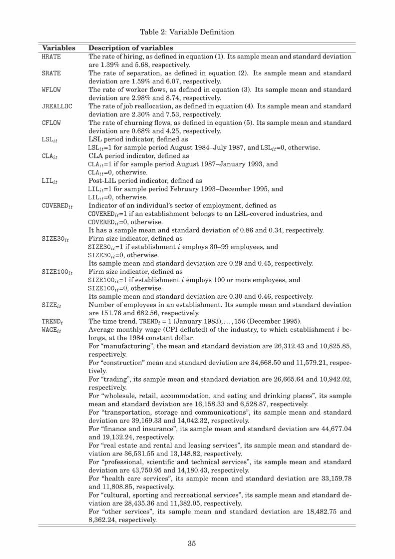
Table 2: Variable Definition

Variables Description of variablesHRATE The rate of hiring, as defined in equation (1). Its sample mean and standard deviation

are 1.39% and 5.68, respectively.SRATE The rate of separation, as defined in equation (2). Its sample mean and standard

deviation are 1.59% and 6.07, respectively.WFLOW The rate of worker flows, as defined in equation (3). Its sample mean and standard

deviation are 2.98% and 8.74, respectively.JREALLOC The rate of job reallocation, as defined in equation (4). Its sample mean and standard

deviation are 2.30% and 7.53, respectively.CFLOW The rate of churning flows, as defined in equation (5). Its sample mean and standard

deviation are 0.68% and 4.25, respectively.LSLit LSL period indicator, defined as

LSLit=1 for sample period August 1984–July 1987, and LSLit=0, otherwise.CLAit CLA period indicator, defined as

CLAit=1 if for sample period August 1987–January 1993, andCLAit=0, otherwise.

LILit Post-LIL period indicator, defined asLILit=1 for sample period February 1993–December 1995, andLILit=0, otherwise.

COVEREDit Indicator of an individual’s sector of employment, defined asCOVEREDit=1 if an establishment belongs to an LSL-covered industries, andCOVEREDit=0, otherwise.It has a sample mean and standard deviation of 0.86 and 0.34, respectively.

SIZE30it Firm size indicator, defined asSIZE30it=1 if establishment i employs 30–99 employees, andSIZE30it=0, otherwise.Its sample mean and standard deviation are 0.29 and 0.45, respectively.

SIZE100it Firm size indicator, defined asSIZE100it=1 if establishment i employs 100 or more employees, andSIZE100it=0, otherwise.Its sample mean and standard deviation are 0.30 and 0.46, respectively.

SIZEit Number of employees in an establishment. Its sample mean and standard deviationare 151.76 and 682.56, respectively.

TRENDt The time trend. TRENDt = 1 (January 1983), . . . ,156 (December 1995).WAGEit Average monthly wage (CPI deflated) of the industry, to which establishment i be-

longs, at the 1984 constant dollar.For “manufacturing”, the mean and standard deviation are 26,312.43 and 10,825.85,respectively.For “construction” mean and standard deviation are 34,668.50 and 11,579.21, respec-tively.For “trading”, its sample mean and standard deviation are 26,665.64 and 10,942.02,respectively.For “wholesale, retail, accommodation, and eating and drinking places”, its samplemean and standard deviation are 16,158.33 and 6,528.87, respectively.For “transportation, storage and communications”, its sample mean and standarddeviation are 39,169.33 and 14,042.32, respectively.For “finance and insurance”, its sample mean and standard deviation are 44,677.04and 19,132.24, respectively.For “real estate and rental and leasing services”, its sample mean and standard de-viation are 36,531.55 and 13,148.82, respectively.For “professional, scientific and technical services”, its sample mean and standarddeviation are 43,750.95 and 14,180.43, respectively.For “health care services”, its sample mean and standard deviation are 33,159.78and 11,808.85, respectively.For “cultural, sporting and recreational services”, its sample mean and standard de-viation are 28,435.36 and 11,382.05, respectively.For “other services”, its sample mean and standard deviation are 18,482.75 and8,362.24, respectively.

35

Table 3: Weighted Average Labor Turnover Rates†

Worker and Job Turnover Rates (%)Period 1–29 Employees 30–99 Employees ≥100 Employees

LSL-Covered Non-Covered LSL-Covered Non-Covered LSL Covered Non-Covered

HRATE 1.05 1.26 3.17 1.33 3.30 1.19(5.50) (6.28) (5.98) (3.43) (5.35) (2.23)

SRATE 1.17 1.62 3.14 1.22 3.16 1.09(5.87) (7.25) (5.80) (3.78) (4.79) (1.99)

WFLOW 2.21 2.89 6.31 2.54 6.45 2.28Pre-LSL (8.37) (9.92) (9.17) (5.58) (8.29) (3.43)

JREALLOC 1.84 2.41 3.65 1.63 3.01 1.19(7.49) (8.93) (6.44) (4.28) (5.04) (2.17)

CFLOW 0.38 0.48 2.66 0.92 3.44 1.10(3.68) (4.50) (5.78) (2.91) (5.91) (2.32)

Observation 38,307 13,221 23,846 3,936 32,469 2,338

HRATE 1.13 0.99 3.15 1.40 3.24 1.22(5.58) (5.70) (5.92) (3.99) (5.31) (2.68)

SRATE 1.16 1.37 3.30 1.27 3.45 1.11(5.61) (6.78) (5.71) (3.82) (5.10) (2.22)

WFLOW 2.29 2.36 6.45 2.67 6.69 2.33LSL (8.38) (9.22) (8.96) (6.01) (8.38) (3.89)

JREALLOC 1.78 1.96 3.83 1.75 3.25 1.26(7.20) (8.27) (6.37) (4.67) (5.26) (2.76)

CFLOW 0.51 0.41 2.62 0.92 3.44 1.07(4.26) (4.19) (5.69) (3.06) (5.99) (2.39)

Observation 70,218 24,505 52,159 8,248 68,798 5,318

HRATE 1.37 0.99 3.08 1.94 3.09 1.82(5.81) (5.44) (5.59) (3.94) (4.87) (3.14)

SRATE 1.63 1.09 3.62 2.05 3.72 1.57(6.35) (5.77) (5.78) (4.17) (5.09) (2.80)

WFLOW 3.00 2.08 6.70 3.99 6.82 3.40CLA (8.93) (8.32) (8.43) (6.42) (7.72) (4.60)

JREALLOC 2.45 1.69 4.26 2.29 3.54 1.82(7.89) (7.33) (6.35) (4.41) (5.24) (3.32)

CFLOW 0.55 0.39 2.44 1.70 3.27 1.58(4.02) (3.99) (5.18) (4.09) (5.39) (2.75)

Observation 155,935 41,248 128,793 13,948 136,672 14,570

HRATE 1.47 0.93 2.68 2.60 2.62 2.42(5.76) (5.16) (5.00) (4.55) (4.45) (4.25)

SRATE 1.70 1.13 2.95 2.49 2.67 2.09(6.14) (5.74) (5.07) (4.34) (4.17) (3.48)

WFLOW 3.17 2.05 5.63 5.09 5.29 4.51LIL (8.86) (8.10) (7.48) (7.10) (6.59) (6.15)

JREALLOC 2.49 1.66 3.66 2.74 2.96 2.11(7.56) (7.12) (5.67) (4.60) (4.71) (4.26)

CFLOW 0.68 0.40 1.97 2.34 2.32 2.40(4.44) (3.81) (4.48) (4.90) (4.25) (3.94)

Observation 85,088 15,542 69,489 6,812 59,581 9,124†Standard deviation in parentheses.

36

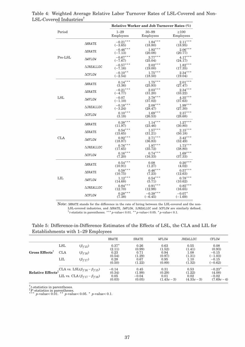
Table 4: Weighted Average Relative Labor Turnover Rates of LSL-Covered and Non-LSL-Covered Industries†

Relative Worker and Job Turnover Rates (%)

Period 1–29 30–99 ≥100Employees Employees Employees

∆HRATE −0.21∗∗∗ 1.84∗∗∗ 2.11∗∗∗(−3.65) (18.80) (18.95)

∆SRATE −0.46∗∗∗ 1.92∗∗∗ 2.06∗∗∗(−7.13) (20.08) (20.77)

Pre-LSL ∆WFLOW −0.67∗∗∗ 3.77∗∗∗ 4.17∗∗∗(−7.67) (25.04) (24.17)

∆JREALLOC −0.57∗∗∗ 2.02∗∗∗ 1.82∗∗∗(−7.16) (19.00) (17.35)

∆CFLOW −0.10∗∗ 1.75∗∗∗ 2.34∗∗∗(−2.54) (18.50) (19.04)

∆HRATE 0.14∗∗∗ 1.75∗∗∗ 2.01∗∗∗(3.36) (25.93) (27.47)

∆SRATE −0.21∗∗∗ 2.03∗∗∗ 2.34∗∗∗(−4.77) (31.20) (33.22)

LSL ∆WFLOW −0.07 3.78∗∗∗ 4.35∗∗∗(−1.10) (37.02) (37.63)

∆JREALLOC −0.18∗∗∗ 2.08∗∗∗ 1.99∗∗∗(−3.24) (28.47) (27.30)

∆CFLOW 0.10∗∗∗ 1.69∗∗∗ 2.37∗∗∗(3.18) (26.53) (28.68)

∆HRATE 0.38∗∗∗ 1.14∗∗∗ 1.27∗∗∗(11.97) (23.46) (30.80)

∆SRATE 0.54∗∗∗ 1.57∗∗∗ 2.15∗∗∗(15.65) (31.21) (50.18)

CLA ∆WFLOW 0.92∗∗∗ 2.71∗∗∗ 3.42∗∗∗(18.87) (36.83) (52.49)

∆JREALLOC 0.76∗∗∗ 1.97∗∗∗ 1.73∗∗∗(17.65) (35.72) (38.80)

∆CFLOW 0.16∗∗∗ 0.74∗∗∗ 1.69∗∗∗(7.20) (16.33) (37.33)

∆HRATE 0.54∗∗∗ 0.08 0.20∗∗∗(10.91) (1.27) (4.02)

∆SRATE 0.58∗∗∗ 0.46∗∗∗ 0.57∗∗∗(10.75) (7.23) (12.63)

LIL ∆WFLOW 1.12∗∗∗ 0.54∗∗∗ 0.78∗∗∗(14.68) (5.71) (10.62)

∆JREALLOC 0.84∗∗∗ 0.91∗∗∗ 0.85∗∗∗(12.70) (12.98) (16.65)

∆CFLOW 0.28∗∗∗ −0.38∗∗∗ −0.07∗(7.38) (−6.45) (−1.69)

Note: ∆HRATE stands for the difference in the rate of hiring between the LSL-covered and the non-LSL-covered industries, and ∆SRATE, ∆WFLOW, ∆JREALLOC and ∆CFLOW are similarly defined.† t-statistic in parentheses. ∗∗∗p-value< 0.01. ∗∗p-value< 0.05. ∗p-value< 0.1.

Table 5: Difference-in-Difference Estimates of the Effects of LSL, the CLA and LIL forEstablishments with 1–29 Employees

HRATE SRATE WFLOW JREALLOC CFLOW

LSL (β f 15) 0.37∗ 0.26 0.63 0.55 0.08(2.11) (0.99) (1.52) (1.41) (0.93)

Gross Effects† CLA (β f 16) 0.23 0.71 0.94 1.08 −0.15(0.54) (1.29) (0.97) (1.31) (−1.03)

LIL (β f 17) 0.28 0.67 0.95 1.10 −0.15(0.50) (1.22) (0.89) (1.32) (−0.62)

CLA vs. LSL(β f 16 −β f 15) −0.14 0.45 0.31 0.53 −0.23∗Relative Effects‡ (0.34) (1.99) (0.29) (1.22) (4.08)

LIL vs. CLA (β f 17 −β f 16) 0.05 −0.04 0.01 0.02 −0.02(0.03) (0.05) (1.43e−3) (4.33e−3) (7.69e−4)

†t-statistics in parentheses.‡F-statistics in parentheses.∗∗∗ p-value< 0.01. ∗∗ p-value< 0.05. ∗ p-value< 0.1.

37

Table 6: Difference-in-Difference Estimates of the Effects of LSL, the CLA and LIL forEstablishments with 30–99 Employees

HRATE SRATE WFLOW JREALLOC CFLOW

LSL (β f 18) −0.58∗∗∗ −0.27 −0.84∗∗ −0.57 −0.27∗∗(−3.46) (−1.11) (−2.21) (−1.64) (−2.21)

Gross Effects† CLA (β f 19) −1.26∗∗ −1.36∗∗ −2.61∗∗ −1.52∗ −1.09∗∗∗(−3.10) (−2.47) (−2.79) (−2.03) (−5.60)

LIL (β f 20) −2.48∗∗∗ −2.68∗∗∗ −5.16∗∗∗ −2.79∗∗∗ −2.37∗∗∗(−4.99) (−3.72) (−4.31) (−3.46) (−5.79)

CLA vs. LSL (β f 19 −β f 18) −0.68∗∗ −1.09∗∗ −1.77∗∗ −0.95 −0.82∗∗∗Relative Effects‡ (5.96) (7.12) (7.50) (2.87) (24.09)

LIL vs. CLA (β f 20 −β f 19) −1.22∗∗∗ −1.32∗∗∗ −2.55∗∗∗ −1.27∗∗∗ −1.28∗∗∗(25.43) (22.13) (21.35) (12.44) (22.08)

†t-statistics in parentheses.‡F-statistics in parentheses.∗∗∗ p-value< 0.01. ∗∗ p-value< 0.05. ∗ p-value< 0.1.

Table 7: Difference-in-Difference Estimates of the Effects of LSL, the CLA and LIL forEstablishments with 100 or more Employees

HRATE SRATE WFLOW JREALLOC CFLOW

LSL (β f 21) −0.55∗ −0.06 −0.61 −0.49 −0.12(−2.04) (−0.20) (−1.17) (−1.32) (−0.51)

Gross Effects† CLA (β f 22) −1.38∗∗ −0.90 −2.28∗∗ −1.65∗∗ −0.63(−2.85) (−1.68) (−2.27) (−2.64) (−1.37)

LIL (β f 23) −2.62∗∗∗ −2.58∗∗∗ −5.20∗∗∗ −2.80∗∗∗ −2.40∗∗∗(−3.97) (−4.52) (−4.32) (−4.68) (−3.41)

CLA vs. LSL (β f 22 −β f 21) −0.83∗∗ −0.84∗∗ −1.67∗∗ −1.16∗∗∗ −0.51Relative Effects‡ (8.01) (8.43) (9.59) (10.85) (3.14)

LIL vs. CLA (β f 23 −β f 22) −1.24∗∗ −1.78∗∗∗ −2.92∗∗∗ −1.15∗∗ −1.77∗∗∗(6.44) (9.88) (9.85) (7.06) (11.09)

†t-statistics in parentheses.‡F-statistics in parentheses.∗∗∗p-value< 0.01. ∗∗p-value< 0.05. ∗p-value< 0.1.

Table 8: Triple-Difference Estimates of the Differential Impacts on Establishments ofDifferent Sizes†

HRATE SRATE WFLOW JREALLOC CFLOW

Establishments employing 30–99 vs. those employing 1–29 employees

Effects of LSL (β f 18 −β f 15) −0.95∗∗ −0.53 −1.47∗ −1.02 −0.35(9.35) (1.31) (4.19) (2.71) (3.13)

Effects of CLA (β f 19 −β f 16) −1.49∗ −2.07∗ −3.55∗ −2.60∗ −1.24∗∗∗(3.76) (4.75) (4.41) (3.41) (10.75)

Effects of LIL (β f 20 −β f 17) −2.76∗∗∗ −3.35∗∗∗ −6.11∗∗∗ −3.89∗∗∗ −2.54∗∗∗(10.79) (13.01) (12.87) (9.97) (19.15)

Establishments employing 100 or more vs. those employing 30–99 employees

Effects of LSL (β f 21 −β f 18) 0.03 0.21 0.23 0.8 0.15(0.01) (0.95) (0.32) (0.14) (0.56)

Effects of CLA (β f 22 −β f 19) −0.12 0.46∗ 0.33 −0.14 0.46(0.34) (3.60) (0.71) (0.27) (1.64)

Effects of LIL (β f 23 −β f 20) −0.14 0.10 −0.04 −0.01 −0.03(0.11) (0.05) (2.27e−3) (9.62e−4) (2.53e−3)

†F-statistics in parentheses.∗∗∗ p-value< 0.01. ∗∗ p-value< 0.05. ∗ p-value< 0.1.

38

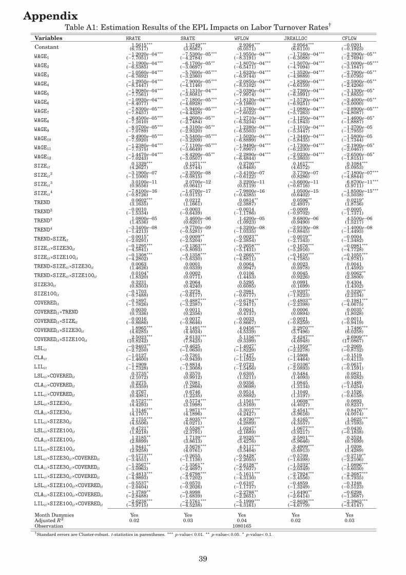
Table A1: Estimation Results of the EPL Impacts on Labor Turnover Rates†Appendix

Variables HRATE SRATE WFLOW JREALLOC CFLOW

Constant 1.5615∗∗∗ 1.3749∗∗∗ 2.9364∗∗∗ 2.9564∗∗∗ −0.0201(6.7517) (3.8567) (6.0571) (6.6110) (−0.1923)

WAGE1−1.2020e−04∗∗∗ −7.5300e−05∗∗∗ −1.9550e−04∗∗∗ −1.7160e−04∗∗∗ −2.3900e−05∗∗

(−7.7051) (−4.2784) (−8.3191) (−6.3088) (−2.7694)WAGE2

−1.1900e−04∗∗∗ −6.1700e−05∗∗ −1.8070e−04∗∗∗ −1.5070e−04∗∗∗ −3.0000e−05∗∗∗(−6.5385) (−3.0697) (−6.5471) (−4.7094) (−3.1847)

WAGE3−1.0560e−04∗∗∗ −5.7600e−05∗∗∗ −1.6320e−04∗∗∗ −1.3520e−04∗∗∗ −2.7900e−05∗∗

(−6.7692) (−3.2360) (−6.9744) (−4.9889) (−3.0795)WAGE4

−1.2950e−04∗∗∗ −7.9000e−05∗∗∗ −2.0850e−04∗∗∗ −1.8260e−04∗∗∗ −2.5900e−05∗∗(−8.1447) (−4.1146) (−8.5102) (−6.6159) (−2.4206)

WAGE5−1.9080e−04∗∗∗ −1.1310e−04∗∗∗ −3.0390e−04∗∗∗ −2.7260e−04∗∗∗ −3.1300e−05∗

(−7.7561) (−3.8081) (−7.9974) (−6.3991) (−1.8855)WAGE6

−1.0930e−04∗∗∗ −7.1800e−05∗∗∗ −1.8120e−04∗∗∗ −1.5720e−04∗∗∗ −2.4000e−05∗∗(−8.4077) (−4.6928) (−9.1980) (−6.9251) (−3.0000)

WAGE7−7.8300e−05∗∗∗ −5.9400e−05∗∗∗ −1.3760e−04∗∗∗ −1.0880e−04∗∗∗ −2.8900e−05∗∗∗

(−7.8457) (−4.4328) (−7.6022) (−5.7263) (−4.8087)WAGE8

−8.4500e−05∗∗∗ −4.2600e−05∗∗ −1.2710e−04∗∗∗ −1.1250e−04∗∗∗ −1.4600e−05∗(−7.1610) (−2.7484) (−6.3234) (−5.1843) (−1.8887)

WAGE9−8.0700e−05∗∗∗ −4.3100e−05∗∗ −1.2380e−04∗∗∗ −1.1010e−04∗∗∗ −1.3700e−05

(−7.0789) (−2.9320) (−6.5503) (−5.3447) (−1.7955)WAGE10

−9.4900e−05∗∗∗ −5.5400e−05∗∗∗ −1.5020e−04∗∗∗ −1.3440e−04∗∗∗ −1.5800e−05(−7.5920) (−3.2209) (−6.8899) (−5.8435) (−1.7344)

WAGE11−1.2380e−04∗∗∗ −7.1100e−05∗∗∗ −1.9490e−04∗∗∗ −1.7300e−04∗∗∗ −2.1900e−05∗

(−7.7375) (−3.6649) (−7.8907) (−6.2230) (−2.0467)WAGE12

−1.4470e−04∗∗∗ −8.4200e−05∗∗ −2.2890e−04∗∗∗ −2.0230e−04∗∗∗ −2.6500e−05∗(−7.0243) (−3.0507) (−6.4844) (−5.3803) (−1.8151)

SIZEit0.1329∗∗∗ 0.1371∗∗∗ 0.2700∗∗∗ 0.1617∗∗∗ 0.1084∗∗∗

(4.2627) (5.5744) (4.8468) (4.6372) (5.0953)SIZEit

2 −3.1900e−07 −2.2500e−08 −3.4100e−07 3.7700e−07 −7.1800e−07∗∗∗(−1.1000) (−0.0815) (−0.6122) (0.8286) (−4.8844)

SIZEit3 3.0100e−11 2.0700e−12 3.2200e−11 −3.6600e−11 6.8700e−11∗∗∗

(0.9556) (0.0641) (0.5119) (−0.6716) (3.9711)SIZEit

4 −7.8100e−16 −1.6700e−17 −7.9800e−16 1.0500e−15 −1.8500e−15∗∗∗(−0.8726) (−0.0175) (−0.4385) (0.6402) (−3.5038)

TREND 0.0602∗∗∗ 0.0212 0.0814∗∗ 0.0596∗∗ 0.0219∗(3.1635) (1.1661) (2.3887) (2.4937) (1.8736)

TREND2 −0.0010 −0.0003 −0.0014 −0.0009 −0.0005(−1.5334) (−0.6439) (−1.1786) (−0.9702) (−1.7371)

TREND3 1.0800e−05 3.4600e−06 1.4200e−05 9.6800e−06 4.5500e−06(1.4536) (0.6201) (1.0923) (0.9490) (1.5217)

TREND4 −3.3400e−08 −9.7700e−09 −4.3200e−08 −2.9100e−08 −1.4000e−08(−1.4213) (−0.5281) (−1.0335) (−0.8845) (−1.4493)

TREND×SIZEit−0.0015∗ −0.0009∗∗ −0.0023∗∗ −0.0019∗∗ −0.0004

(−2.0291) (−2.5204) (−2.3854) (−2.7343) (−1.3482)SIZEit×SIZE30it

−0.1295∗∗∗ −0.1363∗∗∗ −0.2658∗∗∗ −0.1676∗∗∗ −0.0981∗∗∗(−4.5841) (−5.8093) (−5.1431) (−5.2916) (−4.7728)

SIZEit×SIZE100it−0.1308∗∗∗ −0.1358∗∗∗ −0.2665∗∗∗ −0.1610∗∗∗ −0.1055∗∗∗

(−4.2802) (−5.6330) (−4.8811) (−4.7585) (−4.9781)TREND×SIZEit×SIZE30it

0.0063 0.0001 0.0064 0.0023 0.0041(1.4626) (0.0339) (0.9947) (0.5978) (1.4592)

TREND×SIZEit×SIZE100it0.0104∗ 0.0002 0.0106 0.0045 0.0062∗∗

(1.8320) (0.0771) (1.4453) (0.9226) (2.3800)SIZE30it

0.3231 0.2064 0.5295 0.0991 0.4304(0.8303) (0.4240) (0.6085) (0.1699) (1.4302)

SIZE100it−0.1703 −0.2278 −0.3981 −0.9207∗ 0.5226∗∗

(−0.7488) (−0.6177) (−0.6777) (−1.8223) (2.2134)COVEREDit

−0.1897 −0.4887∗∗∗ −0.6784∗∗ −0.4803∗∗ −0.1981∗∗∗(−1.7826) (−3.2387) (−2.9471) (−2.2398) (−4.0675)

COVEREDit×TREND 0.0030 0.0011 0.0041 0.0006 0.0035∗(0.7336) (0.2356) (0.4737) (0.0894) (1.8028)

COVEREDit×SIZEit−0.0016 −0.0017 −0.0033 −0.0021 −0.0011

(−0.8686) (−0.8646) (−0.8667) (−0.8259) (−0.9419)COVEREDit×SIZE30it

1.8965∗∗∗ 2.1491∗∗∗ 4.0456∗∗∗ 2.2970∗∗∗ 1.7486∗∗∗(4.6285) (4.4024) (4.5339) (3.7496) (6.0258)

COVEREDit×SIZE100it2.5023∗∗∗ 2.6133∗∗∗ 5.1156∗∗∗ 2.4247∗∗∗ 2.6909∗∗∗

(10.8242) (7.8425) (9.3399) (4.6948) (17.0867)LSLit

−0.9403∗∗ −0.4625 −1.4027∗ −1.1959∗∗ −0.2069(−2.7250) (−1.0630) (−1.8229) (−2.2278) (−0.8732)

CLAit−1.0127 −0.7301 −1.7427 −1.5908 −0.1519

(−1.4600) (−0.9439) (−1.1932) (−1.4464) (−0.4113)LILit

−1.1909 −0.8814 −2.0723 −2.0106∗ −0.0617(−1.7328) (−1.3008) (−1.5456) (−2.0893) (−0.1591)

LSLit×COVEREDit0.3735∗ 0.2570 0.6305 0.5484 0.0821

(2.1072) (0.9912) (1.5211) (1.4093) (0.9282)CLAit×COVEREDit

0.2275 0.7081 0.9356 1.0845 −0.1489(0.5359) (1.2866) (0.9698) (1.3134) (−1.0254)

LILit×COVEREDit0.2767 0.6746 0.9514 1.1040 −0.1526

(0.4981) (1.2235) (0.8892) (1.3197) (−0.6158)LSLit×SIZE30it

0.5727∗∗∗ 0.5774∗∗∗ 1.1501∗∗∗ 1.0608∗∗∗ 0.0893(4.4293) (3.1998) (3.8169) (4.4027) (0.8237)

CLAit×SIZE30it1.3146∗∗∗ 1.9871∗∗∗ 3.3017∗∗∗ 2.4541∗∗∗ 0.8476∗∗∗

(4.1707) (4.1896) (4.2427) (3.9616) (4.0074)LILit×SIZE30it

2.1755∗∗∗ 2.8035∗∗∗ 4.9790∗∗∗ 3.4165∗∗∗ 1.5625∗∗∗(4.5506) (4.0271) (4.2889) (4.3557) (3.7593)

LSLit×SIZE100it0.4721∗ 0.5526∗∗ 1.0247∗ 1.0677∗∗∗ −0.0430

(1.8218) (2.3791) (2.1689) (3.9217) (−0.1838)CLAit×SIZE100it

1.2185∗∗ 1.7139∗∗∗ 2.9325∗∗∗ 2.5801∗∗∗ 0.3524(2.8899) (3.8613) (3.4276) (5.9646) (0.7699)

LILit×SIZE100it1.9441∗∗ 2.5676∗∗∗ 4.5117∗∗∗ 3.4909∗∗∗ 1.0208

(2.9258) (4.0761) (3.5404) (5.6913) (1.4289)LSLit×SIZE30it×COVEREDit

−0.5773∗∗∗ −0.2655 −0.8428∗ −0.5709 −0.2719∗∗(−3.4551) (−1.1136) (−2.2055) (−1.6398) (−2.2106)

CLAit×SIZE30it×COVEREDit−1.2567∗∗ −1.3561∗∗ −2.6128∗∗ −1.5232∗ −1.0896∗∗∗

(−3.0963) (−2.4697) (−2.7937) (−2.0349) (−5.6030)LILit×SIZE30it×COVEREDit

−2.4813∗∗∗ −2.6798∗∗∗ −5.1611∗∗∗ −2.7924∗∗∗ −2.3687∗∗∗(−4.9893) (−3.7202) (−4.3130) (−3.4556) (−5.7935)

LSLit×SIZE100it×COVEREDit−0.5537∗ −0.0570 −0.6107 −0.4859 −0.1248

(−2.0404) (−0.2026) (−1.1737) (−1.3249) (−0.5123)CLAit×SIZE100it×COVEREDit

−1.3789∗∗ −0.8998 −2.2788∗∗ −1.6490∗∗ −0.6298(−2.8488) (−1.6839) (−2.2651) (−2.6414) (−1.3687)

LILit×SIZE100it×COVEREDit−2.6238∗∗∗ −2.5761∗∗∗ −5.1999∗∗∗ −2.8036∗∗∗ −2.3963∗∗∗

(−3.9715) (−4.5238) (−4.3161) (−4.6779) (−3.4147)

Month Dummies Yes Yes Yes Yes YesAdjusted R2 0.02 0.03 0.04 0.02 0.03Observation 1080165†Standard errors are Cluster-robust. t-statistics in parentheses. ∗∗∗ p-value< 0.01. ∗∗ p-value< 0.05. ∗ p-value< 0.1.

39

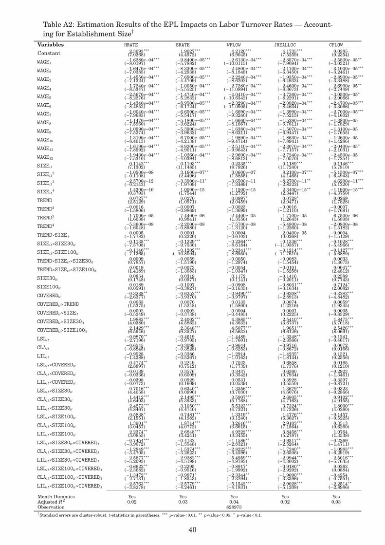
Table A2: Estimation Results of the EPL Impacts on Labor Turnover Rates — Account-ing for Establishment Size†

Variables HRATE SRATE WFLOW JREALLOC CFLOW

Constant 2.3093∗∗∗ 1.9027∗∗∗ 4.2120∗∗∗ 4.1735∗∗∗ 0.0385(7.0268) (4.4572) (6.9045) (7.5259) (0.2354)

WAGE1−1.6280e−04∗∗∗ −9.8400e−05∗∗∗ −2.6130e−04∗∗∗ −2.3570e−04∗∗∗ −2.5500e−05∗∗

(−8.0197) (−5.7882) (−10.0115) (−7.9094) (−3.0321)WAGE2

−1.6470e−04∗∗∗ −8.3300e−05∗∗∗ −2.4800e−04∗∗∗ −2.1700e−04∗∗∗ −3.1000e−05∗∗∗(−7.0385) (−4.2938) (−8.1848) (−6.3450) (−3.2461)

WAGE3−1.4550e−04∗∗∗ −7.6900e−05∗∗∗ −2.2240e−04∗∗∗ −1.9350e−04∗∗∗ −2.8900e−05∗∗∗

(−7.1324) (−4.4709) (−8.6202) (−6.4933) (−3.3488)WAGE4

−1.7240e−04∗∗∗ −1.0050e−04∗∗∗ −2.7280e−04∗∗∗ −2.4600e−04∗∗∗ −2.6900e−05∗∗(−8.5347) (−5.5525) (−11.0894) (−8.3673) (−2.7449)

WAGE5−2.5670e−04∗∗∗ −1.4740e−04∗∗∗ −4.0410e−04∗∗∗ −3.7360e−04∗∗∗ −3.0500e−05∗

(−8.2276) (−5.2832) (−10.6342) (−8.2291) (−2.0066)WAGE6

−1.4340e−04∗∗∗ −8.9500e−05∗∗∗ −2.3290e−04∗∗∗ −2.0820e−04∗∗∗ −2.4700e−05∗∗∗(−8.4852) (−6.1724) (−11.0905) (−8.4634) (−3.3066)

WAGE7−1.0040e−04∗∗∗ −6.6500e−05∗∗∗ −1.6690e−04∗∗∗ −1.3990e−04∗∗∗ −2.7000e−05∗∗∗

(−7.9683) (−5.5417) (−9.3240) (−7.5215) (−4.1602)WAGE8

−1.1470e−04∗∗∗ −5.1800e−05∗∗∗ −1.6660e−04∗∗∗ −1.5280e−04∗∗∗ −1.3800e−05(−7.5960) (−3.6224) (−8.1667) (−6.7611) (−1.7829)

WAGE9−1.0990e−04∗∗∗ −5.3900e−05∗∗∗ −1.6380e−04∗∗∗ −1.5070e−04∗∗∗ −1.3100e−05

(−7.5274) (−3.9632) (−8.6211) (−6.9447) (−1.7655)WAGE10

−1.3190e−04∗∗∗ −6.7000e−05∗∗∗ −1.9890e−04∗∗∗ −1.8630e−04∗∗∗ −1.2600e−05(−8.4013) (−4.2138) (−9.4714) (−7.8941) (−1.4286)

WAGE11−1.6190e−04∗∗∗ −8.9200e−05∗∗∗ −2.5110e−04∗∗∗ −2.3070e−04∗∗∗ −2.0400e−05∗

(−7.8592) (−4.9011) (−9.9643) (−7.7157) (−2.1031)WAGE12

−1.9430e−04∗∗∗ −1.0260e−04∗∗∗ −2.9690e−04∗∗∗ −2.7240e−04∗∗∗ −2.4500e−05(−7.5310) (−4.0394) (−8.6813) (−7.0570) (−1.7254)

SIZEit0.1142∗∗∗ 0.1193∗∗∗ 0.2335∗∗∗ 0.1189∗∗∗ 0.1146∗∗∗

(7.1302) (11.1485) (8.7926) (11.7240) (5.7810)SIZEit

2 −1.0500e−08 3.1600e−07∗∗ 3.0600e−07 8.2100e−07∗∗∗ −5.1500e−07∗∗∗(−0.1108) (2.4496) (1.5855) (4.1465) (−6.4943)

SIZEit3 −2.5700e−12 −3.3900e−11∗ −3.6500e−11 −8.2700e−11∗∗ 4.6200e−11∗∗∗

(−0.2142) (−1.9709) (−1.3469) (−2.8322) (5.1220)SIZEit

4 1.4300e−16 1.0000e−15 1.1500e−15 2.3400e−15∗∗ −1.1900e−15∗∗∗(0.3793) (1.7544) (1.2792) (2.3447) (−4.3750)

TREND 0.0727∗∗ 0.0270 0.0997∗ 0.0728∗ 0.0269(2.5129) (1.0971) (2.0459) (2.0471) (1.7828)

TREND2 −0.0016 −0.0007 −0.0023 −0.0016 −0.0007(−1.5806) (−0.9869) (−1.3699) (−1.2110) (−1.7691)

TREND3 1.7000e−05 7.4400e−06 2.4400e−05 1.7700e−05 6.7500e−06(1.6038) (0.9841) (1.3556) (1.2643) (1.5808)

TREND4 −5.3600e−08 −2.2000e−08 −7.5700e−08 −5.4800e−08 −2.0800e−08(−1.6048) (−0.8980) (−1.3120) (−1.2260) (−1.5182)

TREND×SIZEit−0.0005 0.0001 −0.0004 2.0400e−05 −0.0004

(−1.7782) (0.2220) (−0.6103) (0.0268) (−1.5129)SIZEit×SIZE30it

−0.1135∗∗∗ −0.1229∗∗∗ −0.2364∗∗∗ −0.1336∗∗∗ −0.1028∗∗∗(−7.5708) (−9.7530) (−8.6184) (−11.9367) (−5.4966)

SIZEit×SIZE100it−0.1140∗∗∗ −0.1202∗∗∗ −0.2341∗∗∗ −0.1214∗∗∗ −0.1127∗∗∗

(−7.1365) (−10.8094) (−8.6950) (−11.7610) (−5.6889)TREND×SIZEit×SIZE30it

0.0009 −0.0059 −0.0050 −0.0083 0.0033(0.7857) (−1.5190) (−1.2974) (−1.5454) (1.3073)

TREND×SIZEit×SIZE100it0.0019 −0.0073 −0.0054 −0.0101 0.0047∗∗

(1.4189) (−1.3083) (−1.0347) (−1.5258) (2.4812)SIZE30it

0.0854 0.0319 0.1172 −0.1416 0.2589(0.1748) (0.0577) (0.1141) (−0.2011) (0.7743)

SIZE100it0.0189 −0.1097 −0.0908 −0.8031∗∗∗ 0.7124∗

(0.0591) (−0.3827) (−0.1635) (−3.1634) (2.0082)COVEREDit

−0.3238∗∗ −0.6252∗∗∗ −0.9490∗∗∗ −0.6208∗∗ −0.3282∗∗∗(−2.6377) (−3.9370) (−3.9797) (−2.8913) (−4.8482)

COVEREDit×TREND 0.0063 0.0070 0.0133 0.0074 0.0059∗(1.5375) (1.5248) (1.5800) (1.2216) (1.9345)

COVEREDit×SIZEit−0.0002 −0.0002 −0.0004 0.0001 −0.0005

(−0.5249) (−0.3738) (−0.4485) (0.2225) (−0.8329)COVEREDit×SIZE30it

1.9883∗∗∗ 2.4002∗∗∗ 4.3885∗∗∗ 2.5410∗∗∗ 1.8475∗∗∗(4.0380) (4.5862) (4.3632) (3.6737) (5.7018)

COVEREDit×SIZE100it2.1429∗∗∗ 2.3648∗∗∗ 4.5077∗∗∗ 1.9651∗∗∗ 2.5426∗∗∗

(6.5946) (9.3527) (8.5632) (6.6126) (8.0691)LSLit

−0.9870∗∗ −0.4619 −1.4489 −1.3248∗∗ −0.1241(−2.7196) (−0.9703) (−1.7601) (−2.3566) (−0.4617)

CLAit−0.6545 −0.3099 −0.9644 −0.9716 0.0072

(−0.8845) (−0.3828) (−0.6253) (−0.8672) (0.0166)LILit

−0.9528 −0.3386 −1.2914 −1.4235∗ 0.1321(−1.4288) (−0.5267) (−1.0163) (−1.8144) (0.2556)

LSLit×COVEREDit0.4774∗∗ 0.2249 0.7023 0.6858 0.0165

(2.8897) (0.7512) (1.7739) (1.7376) (0.1210)CLAit×COVEREDit

−0.0139 0.3576 0.3437 0.6360 −0.2923(−0.0336) (0.6009) (0.3542) (0.7934) (−1.3461)

LILit×COVEREDit−0.0398 0.0929 0.0531 0.3928 −0.3397

(−0.0773) (0.1609) (0.0539) (0.5550) (−0.8721)LSLit×SIZE30it

0.7016∗∗∗ 0.6340∗∗ 1.3356∗∗∗ 1.3679∗∗∗ −0.0323(4.4058) (3.0990) (3.7030) (4.6076) (−0.2866)

CLAit×SIZE30it1.4412∗∗∗ 2.1495∗∗∗ 3.5907∗∗∗ 2.6805∗∗∗ 0.9102∗∗∗

(4.6493) (5.3933) (5.1768) (4.7163) (4.9155)LILit×SIZE30it

2.4273∗∗∗ 3.1050∗∗∗ 5.5323∗∗∗ 3.7324∗∗∗ 1.8000∗∗∗(4.8467) (4.4740) (4.7321) (4.7326) (4.0260)

LSLit×SIZE100it0.5838∗ 0.7481∗∗∗ 1.3319∗∗ 1.4776∗∗∗ −0.1457

(2.1551) (4.1982) (3.1240) (6.3627) (−0.5225)CLAit×SIZE100it

1.3901∗∗ 1.8714∗∗∗ 3.2616∗∗∗ 2.9103∗∗∗ 0.3513(3.0457) (4.0772) (3.6615) (7.1564) (0.6260)

LILit×SIZE100it2.2374∗∗ 2.6848∗∗∗ 4.9222∗∗∗ 3.8458∗∗∗ 1.0764

(3.0855) (3.4241) (3.3455) (5.2787) (1.3338)LSLit×SIZE30it×COVEREDit

−0.7454∗∗∗ −0.4132 −1.1586∗∗ −0.9317∗∗ −0.2269(−3.9072) (−1.5548) (−2.8321) (−2.5264) (−1.4711)

CLAit×SIZE30it×COVEREDit−1.2849∗∗∗ −1.5374∗∗∗ −2.8222∗∗∗ −1.7240∗∗ −1.0983∗∗∗

(−3.4705) (−3.2623) (−3.4596) (−2.6506) (−6.2919)LILit×SIZE30it×COVEREDit

−2.5677∗∗∗ −2.9282∗∗∗ −5.4959∗∗∗ −2.9944∗∗∗ −2.5016∗∗∗(−5.2093) (−4.5198) (−4.9783) (−4.3002) (−5.7635)

LSLit×SIZE100it×COVEREDit−0.6622∗∗ −0.2295 −0.8917∗ −0.9180∗∗ 0.0263

(−2.3682) (−0.9516) (−1.9992) (−2.9292) (0.0884)CLAit×SIZE100it×COVEREDit

−1.3472∗∗ −0.9871∗ −2.3344∗∗ −1.9090∗∗∗ −0.4254(−2.7131) (−1.8343) (−2.3294) (−3.3396) (−0.7551)

LILit×SIZE100it×COVEREDit−2.5763∗∗∗ −2.5779∗∗∗ −5.1542∗∗∗ −2.9028∗∗∗ −2.2514∗∗

(−3.8278) (−4.2461) (−4.1831) (−5.1208) (−2.8986)

Month Dummies Yes Yes Yes Yes YesAdjusted R2 0.02 0.03 0.04 0.02 0.03Observation 828973†Standard errors are cluster-robust. t-statistics in parentheses. ∗∗∗ p-value< 0.01. ∗∗ p-value< 0.05. ∗ p-value< 0.1.

40

Table A3: Estimation Results of the EPL Impacts on Labor Turnover Rates—Estimationwith Six-Month Windows†

Variables HRATE SRATE WFLOW JREALLOC CFLOW

Constant 0.0430 −0.9296 −0.8865 −0.4620 −0.4245(0.0791) (−1.6596) (−0.9483) (−0.5903) (−0.4183)

WAGE1−8.3000e−05∗∗∗ −4.7500e−05∗ −1.3050e−04∗∗ −1.1420e−04∗∗ −1.6300e−05∗

(−3.6889) (−2.1889) (−3.0278) (−2.9662) (−2.0924)WAGE2

−8.2400e−05∗∗ −3.6800e−05 −1.1920e−04∗∗ −9.4000e−05∗ −2.5200e−05∗∗(−3.1331) (−1.4431) (−2.3651) (−2.0614) (−2.8932)

WAGE3−6.9000e−05∗∗ −3.6100e−05 −1.0510e−04∗∗ −7.7000e−05∗ −2.8100e−05∗∗∗

(−3.0531) (−1.6560) (−2.4273) (−2.0000) (−3.5346)WAGE4

−8.7100e−05∗∗∗ −5.1100e−05∗ −1.3820e−04∗∗ −1.1750e−04∗∗ −2.0700e−05∗(−3.5121) (−2.1471) (−2.9095) (−2.8245) (−2.1975)

WAGE5−1.2310e−04∗∗∗ −6.6900e−05∗ −1.9000e−04∗∗ −1.6980e−04∗∗ −2.0100e−05

(−3.1564) (−1.8081) (−2.5606) (−2.6244) (−1.3400)WAGE6

−8.8100e−05∗∗∗ −5.4900e−05∗∗ −1.4300e−04∗∗∗ −1.1800e−04∗∗∗ −2.5100e−05∗∗∗(−4.4721) (−2.8594) (−3.7632) (−3.5119) (−3.5105)

WAGE7−7.1800e−05∗∗∗ −5.6200e−05∗∗∗ −1.2810e−04∗∗∗ −9.7300e−05∗∗∗ −3.0700e−05∗∗∗

(−4.3515) (−3.7219) (−4.2987) (−3.7137) (−4.5214)WAGE8

−5.0400e−05∗∗ −1.6900e−05 −6.7300e−05∗ −6.5900e−05∗ −1.4600e−06(−2.5075) (−1.0060) (−1.9339) (−2.1678) (−0.1992)

WAGE9−5.2500e−05∗∗ −1.8900e−05 −7.1400e−05∗ −6.4900e−05∗ −6.4800e−06

(−2.7344) (−1.1386) (−2.1000) (−2.1852) (−0.9191)WAGE10

−6.6700e−05∗∗ −3.5500e−05∗ −1.0220e−04∗∗ −9.8100e−05∗∗ −4.1400e−06(−2.8383) (−1.8783) (−2.5360) (−2.8517) (−0.4381)

WAGE11−9.2100e−05∗∗∗ −5.1300e−05∗ −1.4350e−04∗∗ −1.3490e−04∗∗ −8.6000e−06

(−3.4755) (−2.0685) (−2.8700) (−3.1011) (−0.8431)WAGE12

−9.3600e−05∗∗ −3.8600e−05 −1.3220e−04∗ −1.2210e−04∗ −1.0100e−05(−2.4960) (−1.2293) (−2.0338) (−2.1687) (−0.7163)

SIZEit0.1485∗∗∗ 0.1604∗∗∗ 0.3089∗∗∗ 0.1946∗∗∗ 0.1143∗∗∗

(3.5130) (4.6102) (4.0176) (4.1042) (3.8610)SIZEit

2 −2.9100e−07 −6.2200e−08 −3.5300e−07 2.5600e−07 −6.0900e−07∗∗∗(−0.7012) (−0.1851) (−0.4757) (0.4339) (−3.6250)

SIZEit3 2.6800e−11 3.5800e−12 3.0400e−11 −2.4900e−11 5.5300e−11∗∗∗

(0.6247) (0.0960) (0.3838) (−0.3802) (3.2917)SIZEit

4 −6.8400e−16 −3.3400e−17 −7.1800e−16 7.1900e−16 −1.4400e−15∗∗(−0.5700) (−0.0309) (−0.3191) (0.3764) (−3.0573)

TREND 0.1662∗∗ 0.1687∗∗ 0.3349∗∗ 0.3204∗∗∗ 0.0146(2.8719) (2.6992) (3.0554) (4.2251) (0.1170)

TREND2 −0.0043∗∗∗ −0.0041∗∗ −0.0084∗∗∗ −0.0084∗∗∗ 0.0000(−4.3080) (−2.8283) (−3.8485) (−3.1816) (−0.0010)

TREND3 4.9300e−05∗∗∗ 3.9500e−05∗∗ 8.8800e−05∗∗∗ 9.4400e−05∗∗ −5.6200e−06(5.5581) (2.3235) (3.7311) (2.5934) (−0.1471)

TREND4 −1.8600e−07∗∗∗ −1.2700e−07∗ −3.1300e−07∗∗∗ −3.5000e−07∗∗ 3.7500e−08(−4.9337) (−1.8433) (−3.2469) (−2.2876) (0.2517)

TREND×SIZEit−0.0022 −0.0019 −0.0042 −0.0033 −0.0008

(−1.1872) (−1.6763) (−1.3878) (−1.5616) (−0.9350)SIZEit×SIZE30it

−0.1410∗∗∗ −0.1545∗∗∗ −0.2956∗∗∗ −0.1943∗∗∗ −0.1012∗∗∗(−3.8336) (−4.9801) (−4.3664) (−4.8124) (−3.6868)

SIZEit×SIZE100it−0.1461∗∗∗ −0.1588∗∗∗ −0.3049∗∗∗ −0.1932∗∗∗ −0.1117∗∗∗

(−3.5451) (−4.6589) (−4.0583) (−4.2148) (−3.7994)TREND×SIZEit×SIZE30it

0.0181∗ 0.0173∗∗∗ 0.0354∗∗ 0.0191∗ 0.0163∗∗(1.8895) (3.5138) (2.4991) (2.1694) (3.0150)

TREND×SIZEit×SIZE100it0.0251∗ 0.0193∗∗ 0.0443 0.0238 0.0206∗∗

(1.8079) (2.6762) (2.1349) (1.7152) (2.9588)SIZE30it

0.5696∗ 0.7544∗ 1.3240 0.7834 0.5406∗∗(2.1223) (1.9256) (2.0478) (1.6898) (2.6258)

SIZE100it0.2259 0.5615 0.7874 −0.1415 0.9289∗∗∗

(0.8577) (1.5451) (1.2918) (−0.2367) (4.3992)COVEREDit

−0.0474 −0.0377 −0.0851 −0.1941 0.1090(−0.4081) (−0.2529) (−0.3678) (−1.3636) (1.0175)

COVEREDit×TREND 0.0050 0.0059 0.0109 0.0019 0.0090∗∗(0.8740) (1.2154) (1.0712) (0.2833) (2.5509)

COVEREDit×SIZEit−0.0019 −0.0016 −0.0034 −0.0024 −0.0010

(−0.9648) (−0.9168) (−0.9433) (−0.9332) (−0.9371)COVEREDit×SIZE30it

1.5339∗∗∗ 1.7163∗∗∗ 3.2502∗∗∗ 1.7563∗∗∗ 1.4939∗∗∗(5.5953) (4.4834) (5.0414) (3.9645) (6.9801)

COVEREDit×SIZE100it2.1655∗∗∗ 2.0784∗∗∗ 4.2439∗∗∗ 1.9703∗∗∗ 2.2736∗∗∗

(7.8341) (5.8368) (6.9576) (3.1650) (16.6555)LSLit

−1.0007∗ −0.2547 −1.2554 −1.2928∗∗ 0.0374(−2.0025) (−0.5155) (−1.2905) (−2.2971) (0.0765)

CLAit−0.8390 −0.1915 −1.0305 −1.4308 0.4003

(−1.2020) (−0.3037) (−0.7834) (−1.7547) (0.6992)LILit

−0.0783 0.0543 −0.0240 −0.1853 0.1613(−0.0715) (0.0660) (−0.0134) (−0.1272) (0.2020)

LSLit×COVEREDit0.1868 −0.4833∗ −0.2965 −0.0009 −0.2956∗∗∗

(1.0264) (−2.1800) (−0.7527) (−0.0025) (−3.4498)CLAit×COVEREDit

−0.0834 −0.0427 −0.1261 0.6536 −0.7797∗∗(−0.1682) (−0.1017) (−0.1404) (1.0368) (−2.7930)

LILit×COVEREDit0.1387 −0.0878 0.0508 0.7447 −0.6939

(0.1751) (−0.1626) (0.0398) (0.9524) (−1.3513)LSLit×SIZE30it

0.3708∗∗∗ −0.4307 −0.0599 0.2738 −0.3336∗∗∗(3.1387) (−1.6203) (−0.1629) (0.8958) (−3.5851)

CLAit×SIZE30it0.3021 0.3608 0.6629 0.9999 −0.3369

(0.9877) (0.6056) (0.7634) (1.5029) (−1.2849)LILit×SIZE30it

1.1326∗∗ 1.0208 2.1534 2.0561∗∗ 0.0973(2.3476) (1.2614) (1.7221) (2.2970) (0.2391)

LSLit×SIZE100it0.1830 −0.3264 −0.1434 0.4088 −0.5522∗∗

(0.6012) (−1.3277) (−0.2727) (1.3486) (−2.2791)CLAit×SIZE100it

0.3149 0.2381 0.5531 1.3873∗∗∗ −0.8343∗∗(0.8051) (0.7443) (0.8546) (4.0734) (−2.2240)

LILit×SIZE100it0.4873 0.6414 1.1287 1.8184∗∗ −0.6898

(0.7610) (1.0259) (0.9732) (2.8612) (−1.1134)LSLit×SIZE30it×COVEREDit

−0.7036∗∗∗ 0.2052 −0.4984 −0.2275 −0.2709∗∗(−4.2706) (0.7115) (−1.1719) (−0.6092) (−2.5302)

CLAit×SIZE30it×COVEREDit−0.9937∗∗ −1.0900 −2.0837∗∗ −1.2935∗ −0.7902∗∗

(−2.7536) (−1.7776) (−2.2322) (−1.8917) (−2.8719)LILit×SIZE30it×COVEREDit

−2.3660∗∗∗ −2.5569∗∗ −4.9229∗∗∗ −2.7864∗∗∗ −2.1365∗∗∗(−4.8866) (−3.1153) (−3.9207) (−3.2289) (−5.2006)

LSLit×SIZE100it×COVEREDit−0.7068∗∗ 0.3795 −0.3273 −0.2018 −0.1255

(−2.2471) (1.4484) (−0.5958) (−0.5607) (−0.5087)CLAit×SIZE100it×COVEREDit

−1.3139∗∗∗ −0.6170∗ −1.9309∗∗ −1.4787∗∗∗ −0.4522(−3.1700) (−1.8836) (−2.7994) (−3.9968) (−1.2090)

LILit×SIZE100it×COVEREDit−2.0307∗∗ −2.0497∗∗∗ −4.0804∗∗∗ −2.3273∗∗∗ −1.7530∗∗

(−3.0952) (−3.8557) (−3.7800) (−4.2503) (−2.7760)

Month Dummies Yes Yes Yes Yes YesAdjusted R2 0.02 0.03 0.04 0.02 0.03Observation 283685†Standard errors are Cluster-robust. t-statistics in parentheses. ∗∗∗ p-value< 0.01. ∗∗ p-value< 0.05. ∗ p-value< 0.1.

41

Appendix Not to be Published

Table B1: Difference-in-Difference Estimates of the Effects of LSL, the CLA and LIL forEstablishments with 3–23 Employees—Accounting for Establishment Size

HRATE SRATE WFLOW JREALLOC CFLOW

LSL (β f 15) 0.48∗∗ 0.22 0.70 0.69 0.02(2.89) (0.75) (1.77) (1.74) (0.12)

Gross Effects† CLA (β f 16) −0.01 0.36 0.34 0.64 −0.29(−0.03) (0.60) (0.35) (0.79) (−1.35)

LIL (β f 17) −0.04 0.09 0.05 0.39 −0.34(−0.08) (0.16) (0.05) (0.55) (−0.87)

CLA vs. LSL (β f 16 −β f 15) −0.49∗ 0.14 −0.33 −0.05 −0.31∗Relative Effects‡ (3.33) (0.17) (0.38) (0.01) (3.35)

LIL vs. CLA (β f 17 −β f 16) −0.03 −0.27∗∗ −0.29 −0.25 −0.05(0.01) (4.97) (0.89) (1.27) (0.06)

†t-statistics in parentheses.‡F-statistics in parentheses.∗∗∗ p-value< 0.01. ∗∗ p-value< 0.05. ∗ p-value< 0.1.

Table B2: Difference-in-Difference Estimates of the Effects of LSL, the CLA and LIL forEstablishments with 37–79 Employees—Accounting for Establishment Size

HRATE SRATE WFLOW JREALLOC CFLOW

Gross Effects† LSL (β f 18) −0.75∗∗∗ −0.41 −1.16∗∗ −0.93∗∗ −0.23(−3.91) (−1.55) (−2.83) (−2.53) (−1.47)

CLA (β f 19) −1.28∗∗∗ −1.54∗∗∗ −2.82∗∗∗ −1.72∗∗ −1.10∗∗∗(−3.47) (−3.26) (−3.46) (−2.65) (6.29)

LIL (β f 20) −2.57∗∗∗ −2.93∗∗∗ −5.50∗∗∗ −2.99∗∗∗ −2.50∗∗∗(−5.21) (−4.52) (−4.98) (−4.30) (−5.76)

Relative Effects‡ CLA vs. LSL (β f 19 −β f 18) −0.53∗∗ −1.13∗∗∗ −1.66∗∗∗ −0.79∗ −0.87∗∗∗(5.41) (21.19) (13.15) (4.24) (27.53)

LIL vs. CLA (β f 20 −β f 19) −1.29∗∗∗ −1.39∗∗∗ −2.68∗∗∗ −1.27∗∗∗ −1.40∗∗∗(26.44) (16.06) (21.24) (12.41) (19.90)

†t-statistics in parentheses.‡F-statistics in parentheses.∗∗∗ p-value< 0.01. ∗∗ p-value< 0.05. ∗ p-value< 0.1.

Table B3: Difference-in-Difference Estimates of the Effects of LSL, the CLA and LIL forEstablishments with 121 or more Employees—Accounting for Establishment Size

HRATE SRATE WFLOW JREALLOC CFLOW

LSL (β f 21) −0.66∗∗ −0.23 −0.89∗ −0.92∗∗ 0.03(−2.37) (−0.95) (−2.00) (−2.93) (0.09)

Gross Effects† CLA (β f 22) −1.35∗∗ −0.99∗ −2.33∗∗ −1.91∗∗ −0.43(−2.71) (−1.83) (−2.33) (−3.34) (−0.76)

LIL (β f 23) −2.58∗∗∗ −2.58∗∗∗ −5.15∗∗∗ −2.90∗∗∗ −2.25∗∗(−3.83) (−4.25) (−4.18) (−5.12) (−2.90)

CLA vs. LSL (β f 22 −β f 21) −0.69∗ −0.76∗ −1.44∗ −0.99∗∗ −0.40Relative Effects‡ (3.74) (4.60) (4.22) (6.82) (1.30)

LIL vs. CLA (β f 23 −β f 22) −1.23∗∗ −1.59∗∗∗ −2.82∗∗ −0.99∗∗ −1.82∗∗∗(6.91) (11.15) (9.24) (5.06) (11.93)

†t-statistics in parentheses.‡F-statistics in parentheses.∗∗∗ p-value< 0.01. ∗∗ p-value< 0.05. ∗ p-value< 0.1.

42

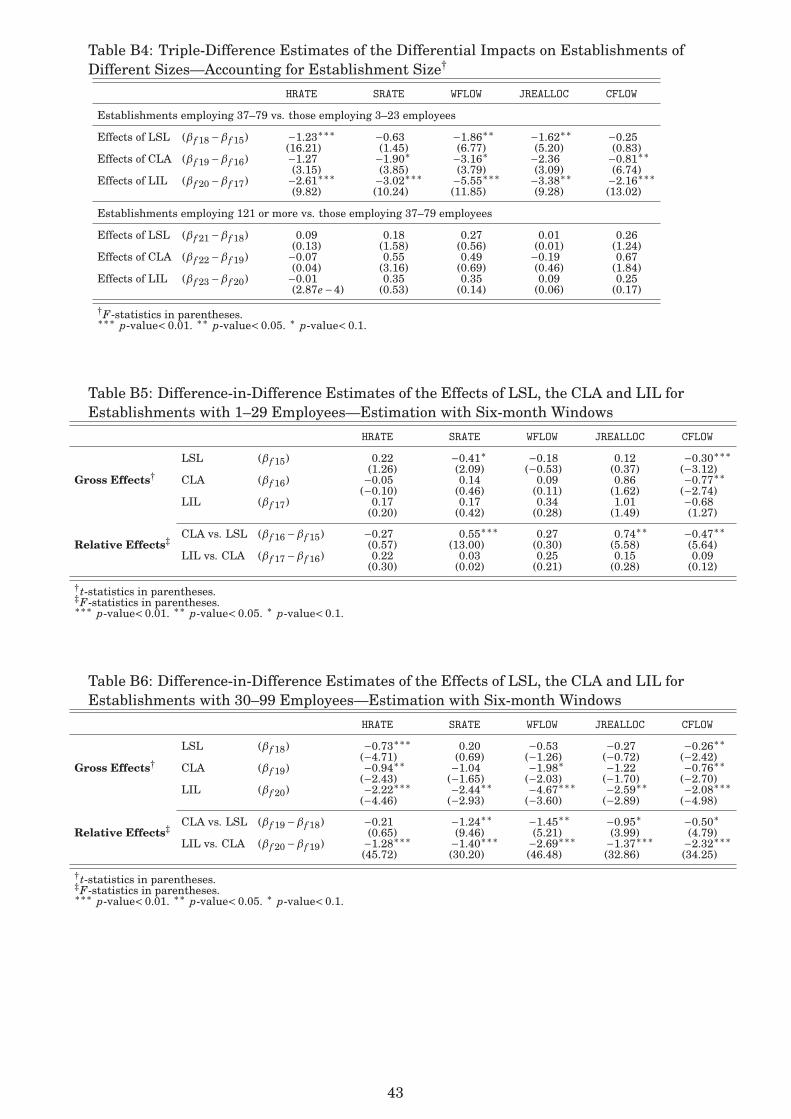
Table B4: Triple-Difference Estimates of the Differential Impacts on Establishments ofDifferent Sizes—Accounting for Establishment Size†

HRATE SRATE WFLOW JREALLOC CFLOW

Establishments employing 37–79 vs. those employing 3–23 employees

Effects of LSL (β f 18 −β f 15) −1.23∗∗∗ −0.63 −1.86∗∗ −1.62∗∗ −0.25(16.21) (1.45) (6.77) (5.20) (0.83)

Effects of CLA (β f 19 −β f 16) −1.27 −1.90∗ −3.16∗ −2.36 −0.81∗∗(3.15) (3.85) (3.79) (3.09) (6.74)

Effects of LIL (β f 20 −β f 17) −2.61∗∗∗ −3.02∗∗∗ −5.55∗∗∗ −3.38∗∗ −2.16∗∗∗(9.82) (10.24) (11.85) (9.28) (13.02)

Establishments employing 121 or more vs. those employing 37–79 employees

Effects of LSL (β f 21 −β f 18) 0.09 0.18 0.27 0.01 0.26(0.13) (1.58) (0.56) (0.01) (1.24)

Effects of CLA (β f 22 −β f 19) −0.07 0.55 0.49 −0.19 0.67(0.04) (3.16) (0.69) (0.46) (1.84)

Effects of LIL (β f 23 −β f 20) −0.01 0.35 0.35 0.09 0.25(2.87e−4) (0.53) (0.14) (0.06) (0.17)

†F-statistics in parentheses.∗∗∗ p-value< 0.01. ∗∗ p-value< 0.05. ∗ p-value< 0.1.

Table B5: Difference-in-Difference Estimates of the Effects of LSL, the CLA and LIL forEstablishments with 1–29 Employees—Estimation with Six-month Windows

HRATE SRATE WFLOW JREALLOC CFLOW

LSL (β f 15) 0.22 −0.41∗ −0.18 0.12 −0.30∗∗∗(1.26) (2.09) (−0.53) (0.37) (−3.12)

Gross Effects† CLA (β f 16) −0.05 0.14 0.09 0.86 −0.77∗∗(−0.10) (0.46) (0.11) (1.62) (−2.74)

LIL (β f 17) 0.17 0.17 0.34 1.01 −0.68(0.20) (0.42) (0.28) (1.49) (1.27)

CLA vs. LSL (β f 16 −β f 15) −0.27 0.55∗∗∗ 0.27 0.74∗∗ −0.47∗∗Relative Effects‡ (0.57) (13.00) (0.30) (5.58) (5.64)

LIL vs. CLA (β f 17 −β f 16) 0.22 0.03 0.25 0.15 0.09(0.30) (0.02) (0.21) (0.28) (0.12)

†t-statistics in parentheses.‡F-statistics in parentheses.∗∗∗ p-value< 0.01. ∗∗ p-value< 0.05. ∗ p-value< 0.1.

Table B6: Difference-in-Difference Estimates of the Effects of LSL, the CLA and LIL forEstablishments with 30–99 Employees—Estimation with Six-month Windows

HRATE SRATE WFLOW JREALLOC CFLOW

LSL (β f 18) −0.73∗∗∗ 0.20 −0.53 −0.27 −0.26∗∗(−4.71) (0.69) (−1.26) (−0.72) (−2.42)

Gross Effects† CLA (β f 19) −0.94∗∗ −1.04 −1.98∗ −1.22 −0.76∗∗(−2.43) (−1.65) (−2.03) (−1.70) (−2.70)

LIL (β f 20) −2.22∗∗∗ −2.44∗∗ −4.67∗∗∗ −2.59∗∗ −2.08∗∗∗(−4.46) (−2.93) (−3.60) (−2.89) (−4.98)

CLA vs. LSL (β f 19 −β f 18) −0.21 −1.24∗∗ −1.45∗∗ −0.95∗ −0.50∗Relative Effects‡ (0.65) (9.46) (5.21) (3.99) (4.79)

LIL vs. CLA (β f 20 −β f 19) −1.28∗∗∗ −1.40∗∗∗ −2.69∗∗∗ −1.37∗∗∗ −2.32∗∗∗(45.72) (30.20) (46.48) (32.86) (34.25)

†t-statistics in parentheses.‡F-statistics in parentheses.∗∗∗ p-value< 0.01. ∗∗ p-value< 0.05. ∗ p-value< 0.1.

43

Table B7: Difference-in-Difference Estimates of the Effects of LSL, the CLA and LIL forEstablishments with 100 or more Employees—Estimation with Six-month Windows

HRATE SRATE WFLOW JREALLOC CFLOW

LSL (β f 21) −0.71∗ 0.39 −0.32 −0.22 −0.11(−2.19) (1.41) (−0.56) (−0.57) (−0.42)

Gross Effects† CLA (β f 22) −1.19∗∗ −0.55 −1.74∗ −1.35∗∗ −0.39(−2.57) (−1.43) (−2.17) (−2.93) (−1.00)

LIL (β f 23) −1.82∗∗ −1.95∗∗∗ −3.77∗∗∗ −2.08∗∗∗ −1.70∗∗(−2.89) (−3.49) (−3.43) (−3.44) (−2.69)

CLA vs. LSL (β f 22 −β f 21) −0.48∗∗ −0.16∗∗∗ −1.42∗∗∗ −1.13∗∗∗ −0.28Relative Effects‡ (6.11) (34.70) (19.74) (27.77) (2.06)

LIL vs. CLA (β f 23 −β f 22) −0.63 −1.40∗∗∗ −2.03∗∗ −0.73∗ −1.31∗∗(2.52) (15.55) (8.19) (4.80) (7.79)

†t-statistics in parentheses.‡F-statistics in parentheses.∗∗∗ p-value< 0.01. ∗∗ p-value< 0.05. ∗ p-value< 0.1.

Table B8: Triple-Difference Estimates of the Differential Impacts on Establishments ofDifferent Sizes—Estimation with Six-month Windows†

HRATE SRATE WFLOW JREALLOC CFLOW

Establishments employing 30–99 vs. those employing 1–29 employees

Effects of LSL (β f 18 −β f 15) −0.95∗∗∗ 0.61 −0.35 −0.39 0.04(10.91) (2.06) (0.26) (0.39) (0.05)

Effects of CLA (β f 19 −β f 16) −0.89 −1.18 −2.07 −2.08∗ 0.01(1.32) (2.49) (2.17) (4.03) (8.17e−4)

Effects of LIL (β f 20 −β f 17) −2.39∗ −2.27∗∗ −5.01∗∗ −3.60∗∗ −1.40∗(4.27) (7.12) (6.71) (8.65) (3.44)

Establishments employing 100 or more vs. those employing 30–99 employees

Effects of LSL (β f 21 −β f 18) 0.02 0.19 0.21 −0.05 0.15(2.15e−3) (1.38) (0.36) (0.06) (0.76)

Effects of CLA (β f 22 −β f 19) −0.25∗ 0.59 0.24 −0.13 0.37(4.06) (2.42) (0.51) (0.13) (2.82)

Effects of LIL (β f 23 −β f 20) 0.40 0.49 0.90 0.51 0.38(1.50) (0.78) (1.52) (1.86) (0.57)

†F-statistics in parentheses.∗∗∗ p-value< 0.01. ∗∗ p-value< 0.05. ∗ p-value< 0.1.

44