the effects of ambient conditions on helicopter rotor source noise modeling · the effects of...
TRANSCRIPT

The Effects of Ambient Conditions onHelicopter Rotor Source Noise Modeling
Eric Greenwood!NASA Langley Research Center
Fredric H. Schmitz†
University of Maryland
A new physics-based method called “Fundamental Rotorcraft Acoustic Modeling from Experiments”(FRAME) is used to demonstrate the change in rotor harmonic noise of a helicopter operating at dif-ferent ambient conditions. FRAME is based upon a non-dimensional representation of the governingacoustic and performance equations of a single rotor helicopter. Measured external noise is used to-gether with parameter identification techniques to develop a model of helicopter external noise that isa hybrid between theory and experiment. The FRAME method is used to evaluate the main rotor har-monic noise of a Bell 206B3 helicopter operating at different altitudes. The variation with altitude ofBlade-Vortex Interaction (BVI) noise, known to be a strong function of the helicopter’s advance ratio,is dependent upon which definition of airspeed is flown by the pilot. If normal flight procedures are fol-lowed and indicated airspeed (IAS) is held constant, the true airspeed (TAS) of the helicopter increaseswith altitude. This causes an increase in advance ratio and a decrease in the speed of sound whichresults in large changes to BVI noise levels. Results also show that thickness noise on this helicopterbecomes more intense at high altitudes where advancing tip Mach number increases because the speedof sound is decreasing and advance ratio increasing for the same indicated airspeed. These resultssuggest that existing measurement-based empirically derived helicopter rotor noise source models maygive incorrect noise estimates when they are used at conditions where data were not measured and mayneed to be corrected for mission land-use planning purposes.
Notation
A Rotor Disk Areaa0 Ambient Speed of Soundax Longitudinal Acceleration of Aircraftb Number of Rotor Bladescd0 Blade Element Profile Drag CoefficientCT Thrust CoefficientCp" Acoustic Pressure CoefficientCpi j Blade Surface Pressure CoefficientCL Mean Blade Section Lift CoefficientD f Fuselage Parasite Dragfe Effective Flag Plate Drag Areag Gravitational AccelerationH Rotor Longitudinal “H-Force”M Section Mach NumberMAT Advancing Tip Mach NumberMH Hover Tip Mach NumberMr Mach Number along Propagation Directionn Surface Normal DirectionP Surface Pressurep" Acoustic Perturbation Pressure
!Research Aerospace Engineer, [email protected]†Senior Research Professor, [email protected]
Presented at the American Helicopter Society 67th Annual Forum,Virginia Beach, VA, May 3-5, 2011. This is a work of the U.S.Government and is not subject to copyright protection in the U.S.
Q Lighthill Stress Tensorr Propagation Distancer Non-Dimensional Propagation Distancer Non-Dimensional Radial StationR Rotor RadiusR! Molar Mass of AirS Blade Surface Areat Time of Observationt Non-Dimensional Time of ObservationT0 Ambient TemperatureU Blade Section Velocity relative to MediumV Aircraft Velocity Relative to Mediumvi Mean Induced VelocityVIAS Indicated Airspeedvn Velocity of Medium Normal to Blade SurfaceW Vehicle Gross Weightx Cartesian Coordinate Vectorx Non-Dimensional Cartesian Coordinate Vector
!T PP Tip-Path-Plane Angle of Attack! Tip Vortex Circulation Strength" Flight Path Angle"! Adiabatic Coefficient of Air# Inflow Ratioµ Advance Ratio$ Airfoil Surface Slope%0 Ambient Density
https://ntrs.nasa.gov/search.jsp?R=20110011597 2018-10-15T18:48:32+00:00Z

%SL Ambient Density at Sea Level& Rotor Solidity' Time of Emission' Non-Dimensional Time of Emission( Wake Skew Ratio) Rotor Azimuth" Rotor Rotational Speed
Introduction
Helicopter acoustic land-use and mission planning tools aregaining favor for both military and commercial applica-tions. For the military, reducing the detection distance (thedistance when an observer first notices the vehicle) is nor-mally the focus. In commercial applications, there is alsointerest in the detection or noticeability of rotorcraft noise,especially in areas with low ambient noise levels such asrural parks; however, the primary civil focus is designinghelicopter operations which reduce community annoyancecaused by exposure to helicopter noise. For any of theseapplications, accurate noise models are needed in order toestimate the acoustic impact of helicopter operations on theobservers.
Noise modeling in land-use and mission planning toolsis composed of three distinct components: a noise sourcemodel, a propagation model, and a receiver model. Thenoise source model characterizes the far-field noise radia-tion of the helicopter. The magnitude and direction of ro-tor noise is strongly dependent on the operating conditionof the helicopter, so the external noise radiation must be afunction of the helicopter operating state. The propagationmodel estimates how the sound radiated by the helicopterwill propagate through the atmosphere and around terrainto the locations of the observers, and is a strong functionof the environmental conditions and terrain. The observermodel characterizes the observer characteristics that are im-portant for detection or annoyance.
The focus of this paper is on improving helicopter noisesource modeling. Without an accurate description of noiseradiated at the source, the acoustic impact of helicopter op-erations on observers cannot be accurately predicted. Exist-ing empirical noise models are normally based upon acous-tic measurements of specific helicopters that are flown insteady-state conditions over a ground-based microphonemeasurement array. The measured acoustic data are thenback-propagated to an assumed point of radiation in order toform a compact helicopter source noise model that is validat the chosen operating condition of the specific helicopter.This measurement and modeling process is repeated for anumber of steady operating conditions, with the acousticdata stored as a function of the specific operating condition.An empirical helicopter noise source model is constructedfrom this data set which describes the magnitude and direc-tion of radiated noise as a function of the helicopter oper-
ating condition. Estimating the noise radiation of this he-licopter flying under the measured operating conditions re-verses this process and should result in the reproduction ofthe measured data used to construct the noise source modelat that condition.
Several empirical helicopter source noise modelingmethods are currently in use. The simplest is derivedfrom simple noise-power-distance extrapolations of mea-sured data at a few microphone locations in order to capturesome information about the directivity of helicopter noise.(Refs. 1, 2) More complex modeling methods are based ona linear (Refs. 3–5) or planar (Refs. 6, 7) grid of groundbased microphones—with the most complex of these meth-ods measuring the radiated noise from maneuvering heli-copter in many directions simultaneously using a dense ar-ray of microphone positions on the ground. (Ref. 7) All ofthese modeling approaches have one thing in common—they are based upon acoustic measurements at one ambientoperating condition. Changes in that ambient condition areeither not considered or are accounted for indirectly (andperhaps incorrectly) through changes in the other dependentparameters.
Existing land-use and mission planning tools, such asthe widely used Rotorcraft Noise Model (RNM), (Refs. 3,4)also neglect the effects of ambient conditions on the he-licopter source noise models. The Federal Aviation Ad-ministration’s Integrated Noise Model (INM) (Refs. 1, 2)does include an empirical correction to data measured dur-ing the reference flyover flight condition based on the non-dimensional advancing tip Mach number; this is used to ad-just the source noise level of the measured flight conditionfor airspeeds other than that measured, but since the cor-rection is formulated in terms of the non-dimensional ad-vancing tip Mach number, it also includes the effect of tem-perature changes by way of changes in the ambient speedof sound. However, the simple 2nd order polynomial curvefit used by the INM method does not fully account for thechanges in rotorcraft noise sources due to both flight andambient condition changes, nor can the integrated model-ing method capture changes in the directivity of noise dueto changes in operating condition. (Ref. 8)
Objective
The main objective of this paper is to improve the under-standing of the effects of ambient conditions on helicopterexternal noise radiation using a non-dimensional analyti-cal model of main rotor harmonic noise. A new physics-based experimental method called “Fundamental RotorcraftAcoustic Modeling from Experiments” (FRAME) is usedto assess the acoustic radiation of an example helicopteroperating at altitude. The operational, land-use and mis-sion planning implications of ambient conditions on sourcenoise modeling are also briefly addressed.

Operations at Altitude and the Standard Atmosphere
Helicopters are strongly influenced by ambient conditionsand those conditions are strongly affected by increases inoperating altitude. Temperature, density, and ambient pres-sure all decrease with increasing altitude—this is shown inthe top plot of Figure 1, in accordance with the InternationalStandard Atmosphere (ISA) model. (Ref. 9) These changesaffect helicopter performance and noise, usually in an ad-verse manner.
At altitude, the air is thinner and the temperature de-creases. Lower air density forces the helicopter to operateat high blade lift coefficients that can decrease performanceand increase the likelihood the blade will stall. The lowertemperature also increases the operating Mach number ofthe rotor—again decreasing performance. The aerodynam-ics of the rotor influence noise radiation. Although the pilotmay maintain the same flight condition, as indicated by theaircraft’s instruments, the aerodynamic and acoustic state ofthe rotor will change.
Dimensionally-Defined Flight Conditions
Flight conditions are typically defined by pilots using di-mensional parameters, i.e. indicated airspeed (IAS) andflight path angle. Likewise, these parameters are often usedto define the operating condition of the helicopter during theconstruction and usage of empirical helicopter source noisemodels. However, for a given indicated airspeed and flightpath angle, the non-dimensional parameters that are knownto govern rotor harmonic noise vary with ambient densityand speed of sound. In this paper, the governing parametersused to define the rotor operating condition are the advanceratio (µ), wake skew ratio ((), thrust coefficient (CT ), andhover tip Mach number (MH ). The definition and physi-cal relevance of these parameters is explained in AppendixI. The effect of this variation in ambient conditions on thenon-dimensional operating condition of a helicopter rotor isillustrated in lower two plots of Figure 1 for a flight condi-tion defined by a constant set of dimensional parameters—in particular, for a Bell 206B3 operating at a -6.0# flight pathangle and 60 kts IAS at a variety of ISA altitude conditions.
The variation in governing parameters with ambientconditions leads to a changes in the aerodynamic and acous-tic state of the rotor. As air density decreases with in-creasing altitude, the non-dimensional thrust coefficient in-creases, bringing the rotor blades closer to stall and increas-ing the circulation strength of the trailed tip vortices whichform the rotor wake. This also leads to an increase in theinduced inflow through the rotor. In addition, the decreasedair density causes the rotor advance ratio with respect to themedium to increase as true airspeed increases for the sameindicated airspeed. This change in advance ratio results in achange in the epicycloidal pattern of the wake; for exampleFigure 2 shows the “top-view” geometry of the wake for the
0 5000 10000 1500040
60
80
100
0 5000 10000 1500080
100
120
140
Perc
ent of S
ea L
eve
l Valu
e
0 5000 10000 1500050
100
150
200
Altitude, ft
CT
MH
Density
Speed of Sound
Ambient Pressure
µ
!
Fig. 1. (top) The variation in atmospheric and govern-ing parameters for the ISA model. (mid/bottom) Cor-responding variations in the non-dimensional governingparameters for a constant 60 kts IAS -6# FPA approach.
advance ratios associated with 60 kts IAS flight under sealevel and at 15,000 ft ISA altitude conditions. While safetyof flight considerations dictate that pilots fly the helicopterwith respect to indicated airspeed, for noise modeling pur-poses, true airspeed could be used to define the helicopterflight condition. This is equivalent to holding advanced ra-tio fixed. The effects of this approach are considered inAppendix II.
The increase in the rotor induced inflow with altitudedue to the decrease in ambient air density is matched by theincrease in advance ratio for the same indicated airspeed.Therefore, the wake skew ratio remains unchanged with al-titude for a flight condition maintaining constant indicatedairspeed. However, the wake skew ratio will vary with alti-tude for a constant true airspeed flight condition. The wakeskew ratio is related to the average “miss-distance” betweenthe vortices and blades, and is consequently a significant pa-rameter governing Blade-Vortex Interactions (BVI). Lastly,due to the decrease in ambient temperature with altitude,the speed of sound decreases, leading to an increase in therotor tip Mach number. Altogether, these effects result in asignificant change in the rotor acoustic state with variationin altitude that is not accounted for in any of the empiricalrotor noise modeling methods currently in use, all of whichare developed on the basis of dimensional performance pa-rameters.

!1 !0.5 0 0.5 1!1
!0.8
!0.6
!0.4
!0.2
0
0.2
0.4
0.6
0.8
1
x/R
y/R
Sea Level
ISA 15,000 ft
Fig. 2. “Top-view” epicycloidal wake geometry for sealevel and ISA 15,000 ft advance ratios at 60 kts IAS.
Fundamental Rotorcraft Acoustic Modelingfrom Experiments
The Fundamental Rotorcraft Acoustic Modeling from Ex-periments (FRAME) methodology (Ref. 10), previously de-veloped by the authors, is used in this paper to describethe external noise radiation of the Bell 206B3 helicopter.FRAME develops non-dimensional semi-empirical noisesource models for specific helicopters from measured data.A flowchart of the method is shown in Figure 3. Both windtunnel and flight test measurements are used in the model-ing building process. Wind tunnel measurements allow formore careful control of the operating state of the rotor overa wide range of operating conditions, but are usually limitedto scale models of isolated rotors. Flight test measurementsare necessary to acquire noise data for the entire full-sizevehicle, but for practical reasons the variations in operatingcondition are limited.
In the FRAME method, both types of experimentalmeasurements of rotor noise are first classified by oper-ating condition in terms of the non-dimensional govern-ing parameters of rotor harmonic noise. For flight testmeasurements of an entire vehicle, the acoustic signalsare transformed to a wind-tunnel reference frame using atime-domain de-Dopplerization technique. (Ref. 11) Peri-odic averaging is then used to separate the contributionsof main rotor, tail rotor, and non-rotor harmonic noisesources from the transformed signal. Using a parame-ter identification technique, analytical models of the rotornoise sources are then adapted to the acoustic measure-ments by adjusting a set of physics-based dependent mod-eling parameters to match the noise radiated for each setof non-dimensional governing parameters. Application ofthe method across a wide range of operating conditions re-
Relate Dependent Modeling
Parameters to Governing
Parameters
(Neural Network)
Flight Test
Vehicle
Measurments
Non-
Dimensional
Analytical
Model
Define Operating
Conditions by
Non-Dimensional
Governing
Parameters of
Each Type of
Noise SourceMain, Tail and Non-
Rotor Harmonic Noise
Separation
Wind Tunnel
Rotor
Measurements
Identification of
Dependent
Modeling
Parameters for
Each Condition
Identification of
Dependent
Modeling
Parameters for
each Condition
Fig. 3. A flowchart describing the FRAME method fordeveloping rotorcraft source noise models.
sults in a set of dependent modeling parameters associatedwith the non-dimensional governing parameters of the ro-tor noise sources. Using the dependent modeling param-eters developed from both flight test measurements of fullvehicles and wind tunnel measurements of isolated rotors,a neural network model is employed to develop a func-tional relationship between the non-dimensional governingand dependent modeling parameters over the entire rangeof operating conditions. By combining the neural networkparameter estimator with the associated analytical model,estimates of noise at other operating conditions than thosemeasured may be made. In this paper a FRAME model isconstructed for the Bell 206B3 helicopter using a combina-tion of flight test data of the Bell 206B3 (Ref. 12) and windtunnel data from the similar Operational Loads Survey rotortested in the German-Dutch Windtunnel (DNW). (Ref. 13)
The underlying analytical framework used in theFRAME model employs a Ffowcs Williams – Hawkings(FW-H) acoustic analogy method. Aerodynamic inputs areprovided for each condition using a tunable prescribed wakemodel combined with an incompressible indicial unsteadyaerodynamics model. The non-dimensionalized form of theequation (Eq. 2 in Appendix I) is solved numerically usingFarassat Formulation 1A. (Ref. 14) Acoustic sources off theblade surfaces, such as those causing High Speed Impul-sive (HSI) noise, are neglected for the moderate advanc-ing tip Mach number range examined in this paper. Thick-ness noise is directly computed from the blade geometryand rotor operating condition. Loading noise, both lowerharmonic and BVI noise, are determined from an assumedaerodynamic model adapted to measured data using param-eter identification techniques. The lower harmonic loadingvariations required to match the measured data are deter-mined directly, but the higher harmonic loading responsiblefor impulsive BVI noise is found by fitting an adjustablewake model.

The wake model is based on a modified Beddoes pre-scribed wake (Refs. 15, 16) , where the dependent param-eters adjusted by the FRAME method are used to describethe non-uniform longitudinal and lateral inflow variationsacross the rotor disk, the initial vortex core size and its rateof growth (Ref. 17), the tip vortex rollup radius and the rateof wake contraction (Ref. 18), and the harmonic variation ofvortex circulation strength about the rotor azimuth. The ve-locities induced by the wake onto the rotor blades are thencorrected using the Beddoes-Leishman indicial aerodynam-ics model (Refs. 19,20) to account for the delayed responseof the shed wake on the rapidly changing aerodynamic load-ing felt by the blade elements. This is similar to the analyti-cal modeling used in previous theoretical research into BVInoise, (Ref. 21) but with additional physics-based wake dis-tortion terms to allow the model to be accurately fitted to themeasured acoustic data.
Once the fitting process is completed for the entire setof measured data from both the wind tunnel and flight tests,the variations of the dependent parameters with respect tothe governing parameters are incorporated into a single ar-tificial neural network model. The result is a single semi-empirical model of the Bell 206B3 which is applicable overa wide range of operating conditions defined in terms of thefour non-dimensional governing parameters. This modelcan then be used to generate acoustic hemispheres repre-senting the noise radiated by the rotor for various non-dimensionally defined operating conditions, including theeffects of ambient condition variations. In this paper noiseradiation is described using acoustic hemispheres whichshow the far-field noise levels normalized to a fixed dis-tance of 30 ft from the main rotor hub. For BVI noise,the levels shown are calculated using the BVISPL metric,which is the unweighted sound pressure level of all mainrotor harmonic noise from the 6th through 40th harmonicsof the blade passage frequency. For lower harmonic noise,both steady loading and thickness, the unweighted OASPLacross the entire audible frequency range is calculated. Theresulting acoustic hemispheres are plotted using a Lambertconformal conic projection. (Ref. 22)
Results
Steady Loading Noise
First, consider the simple case of a hovering helicopter,where the constant aerodynamic lift is distributed linearlyalong the blade span, and the corresponding induced dragcalculated under the assumption of uniform inflow. Figure4 shows the OASPL hemisphere representation of the noiseradiated by the helicopter at sea level–as expected for steadyloading noise in hover, there is no azimuthal directional-ity to the noise. The OASPL noise metric is used becausethis noise source is known to be dominated by the funda-mental frequency, with noise levels decaying rapidly withhigher frequency harmonics. Figure 5 shows the steady
75
85
95
105
115
0o
270 o
180
o
90o
0 o
!90 o
!60 o !
30 o
0 o
OA
SP
L,dB
Fig. 4. Hovering flight steady loading noise OASPLhemisphere at ISA sea level conditions.(CT = 0.0029 , MH = 0.66)
loading noise hemisphere estimated for the 15,000 ft ISAaltitude condition, where thrust coefficient has increased forthe same vehicle gross weight, due to a decrease in density,and hover tip Mach number has increased for the same ro-tor rotational rate, due to the decrease in the speed of sound.In addition, the ambient pressure decreases as a function ofboth ambient speed of sound and density, as per Equation 5in Appendix I. There is a slight increase in OASPL with al-titude, but no change in directivity. The changes in ambientconditions, hover tip Mach number and thrust coefficientare the same in the hover condition as those shown in Fig-ure 1 for forward flight.
Having a non-dimensional analytical model of the ro-tor harmonic noise sources allows the governing parametervariations to be assessed in isolation from one another, pro-
75
85
95
105
115
0o
270 o
180
o
90o
0 o
!90 o
!60 o !
30 o
0 o
OA
SP
L,dB
Fig. 5. Hovering flight steady loading noise OASPLhemisphere at ISA 15,000 ft altitude conditions.(CT = 0.0046 , MH = 0.70)

0 5000 10000 1500091
92
93
94
95
96
97
98
99
100
101
Altitude, ft
OA
SP
L,
dB
Overa l l
Cp!
CT
MH
Fig. 6. (a) Variation in steady loading noise OASPL(blue) with ISA altitude conditions. (b) OASPL vari-ations associated with individual governing parametervariations with ISA altitude conditions.viding some physical insight into the mechanisms whichlead to changes in noise radiation. Figure 6 plots in blue thevariations in the maximum steady loading noise OASPL ra-diated in any direction with altitude, for ISA ambient con-ditions from those associated with sea level to 15,000 ft al-titude. In addition, the variations in OASPL are shown forcases where only one parameter is allowed to vary accord-ing to ISA conditions, and the rest held fixed at their sealevel values. The change in ambient pressure leads to a sig-nificant reduction in noise levels when the other parameters,including CT , are held fixed. Of course, this is not a phys-ically realizable situation, because the reduction in densityleads to a reduction in dynamic pressure, and hence lift; CTmust be increased to provide the same thrust at altitude. Theincrease in CT associated leads to an increase in noise whichcancels much of the effect of the reduction in ambient pres-sure. The increase in hover tip Mach number with altitudeleads to a moderate increase in noise levels. In total, there isa small increase in noise with altitude for this simple steadyloading source.
Thickness Noise
Thickness noise, like all other rotor harmonic noise sources,is also affected by changes in ambient conditions. From thenon-dimensionalized FW-H equation (Eq. 2 in Appendix I),it is apparent that thickness noise is not governed by param-eters that only affect rotor loading, like thrust coefficientand inflow ratio. Therefore, given a description of the rotorgeometry, thickness noise can be predicted knowing onlythe ambient pressure and blade motion through the medium,which is effectively described by the hover tip Mach num-ber and advance ratio. Figure 7 shows the predicted OASPLacoustic hemisphere for thickness noise produced by theBell 206B3 main rotor during 60kts IAS flight. Indicated
!"#
$"#
%"#
&'"
&&"
###'(
#)!' (
#&$'(
##%'(
###' (
##!%' (
##!*' (##!
+' (
####' (
OA
SP
L,dB
Fig. 7. 60kts IAS OASPL hemisphere of thickness noiseat ISA sea level conditions.(µ = 0.14 , MH = 0.66 , MAT = 0.66)
airspeed (IAS) is chosen as an independent parameter in thisanalysis because it is the airspeed that is normally flown bypilots in order to keep the helicopter within flight safety lim-its. Thickness noise radiates in-plane ahead of and towardthe advancing side of the rotor for any forward flight con-dition. Likewise, Figure 8 shows the thickness noise hemi-sphere predicted for the same dimensionally defined flightcondition at an ISA 15,000 ft altitude ambient conditions.Predictably, the directivity has not changed substantially,but noise levels have increased. Figure 9 shows the trend inpeak thickness noise OASPL with altitude for standard ISAconditions for several different indicated airspeeds. Thick-ness noise increases more rapidly with increasing altitudefor conditions at higher airspeeds.
!"#
$"#
%"#
&'"
&&"
###'(
#)!' (
#&$'(
##%'(
###' (
##!%' (
##!*' (##!
+' (
####' (
OA
SP
L,dB
Fig. 8. 60kts IAS OASPL hemisphere of thickness noiseat ISA 15,000 ft altitude conditions.(µ = 0.18 , MH = 0.70 , MAT = 0.89)

0 5000 10000 15000100
105
110
115
120
125
Altitude, ft
OA
SP
L,
dB
100 kts IAS
80 kts IAS
60 kts IAS
Fig. 9. Peak OASPL thickness noise level variation forISA altitude conditions for constant IAS flight.
0 5000 10000 1500096
98
100
102
104
106
108
Altitude, ft
OA
SP
L,
dB
100 kts IAS
80 kts IAS
60 kts IAS
Fig. 10. OASPL variation in thickness noise for ambientpressure variation per ISA altitude conditions.
As for the steady loading case, the contributions of thegoverning parameters to variation in noise levels can be as-sessed independently. Figure 10 illustrates the variation inthickness noise due to a decrease in ambient pressure due toaltitude, with the sea level values of the advance ratio andhover tip Mach number held fixed. The decrease in ambientpressure leads to a decrease in noise levels, and the effectis proportionate for all cases. (This variation is describedby Equation 5 in Appendix I.) The variation in thicknessnoise with only hover tip Mach number varying in accor-dance to the ISA altitude conditions is shown in Figure 11.As should be expected, the increase in hover tip Mach num-ber with altitude causes a similar increase in thickness noisefor all three indicated airspeeds.
Figure 12 shows the variation in thickness noise withonly the advance ratio varying in order to maintain the sameindicated airspeed (IAS) as density decreases with altitude.
0 5000 10000 15000100
102
104
106
108
110
112
Altitude, ft
OA
SP
L,
dB
100 kts IAS
80 kts IAS
60 kts IAS
Fig. 11. Thickness noise OASPL trend for hover tipMach number variation with temperature at altitude.
0 5000 10000 15000100
102
104
106
108
110
112
114
116
118
Altitude, ft
OA
SP
L,
dB
100 kts IAS
80 kts IAS
60 kts IAS
Fig. 12. Thickness noise OASPL trend for advance ratiovariation to maintain constant IAS at altitude.
An increase in the advance ratio for the same hover tipMach number corresponds to an increase in the advanc-ing tip Mach number. (See Equation 11 in Appendix I.)The increase in advancing tip Mach number leads to a sub-stantial increase in thickness noise levels. The increase innoise levels with altitude is greater for higher indicated air-speeds. The simple monopole thickness noise calculationused in the FRAME analytical model is known to under-predict noise levels at high advancing tip Mach numbers;the increase in noise with altitude when flying constant in-dicated airspeed is likely to be even higher in reality thanpredicted in this paper for high flight speeds.
Blade-Vortex Interaction Noise
Blade-vortex interaction noise is a special case of load-ing noise, and is much more complex. The full FRAME

!"#
$"#
%"#
&'"
&&"
###'(
#)!' (#&$'(
##%'(
###' (
##!%' (
##!*' (##!
+' (
####' (
BV
ISP
L,dB
Fig. 13. 60kts IAS -6# descent BVISPL hemisphere atISA sea level conditions.(µ = 0.14 , ( = 0.046 ,CT = 0.0029 , MH = 0.66)model described previously is used to show effects of am-bient condition variations on BVI noise. Figure 13 showsthe BVISPL contours on the surface of a 30 ft radiusacoustic hemisphere produced by the Bell 206B3 main ro-tor FRAME model for a typical 60 kts indicated airspeed(IAS), -6# flight path angle approach condition, known forhigh levels of BVI noise in standard sea level conditions.Two BVI radiate towards the advancing side: the dominantone radiates towards 120# azimuth and the weaker one to-wards 160# azimuth. In addition, a weak BVISPL “hotspot”can be observed on the retreating side of the rotor at 290#azimuth.
Figure 14 shows a similar BVISPL hemisphere for thesame flight condition at ambient conditions correspondingto a 5,000 ft ISA altitude. While all three BVI ”hotspots”are still present, the magnitude of the BVI hotspots hasincreased. The increase in noise levels is not uniform;the noise radiated by the foremost advancing side BVISPLhotspot has increased more rapidly than the others. In addi-tion, the advancing side BVISPL “hotspots” have shifted indirection further towards the advancing side of the rotor.
Figure 15 shows the hemisphere predicted by the modelfor the same dimensionally defined flight condition at a10,000 ft ISA altitude. The BVI “hotspot” closer to theretreating side has increased further in level. On the ad-vancing side the foremost “hotspot” has increased evenmore in BVISPL, dominating the rearmost advancing side“hotspot.”
The 15,000 ft ISA altitude BVISPL hemisphere pre-dicted by the FRAME model is shown in Figure 16.BVISPL levels increase even further, but this time it is theadvancing side level which increases the most. Both theadvancing and retreating side “hotspots” shift rearward.
The retreating side BVISPL levels continue to decreasewith further increases in altitude. Figure 17 shows the
!"#
$"#
%"#
&'"
&&"
###'(
#)!' (
#&$'(
##%'(
###' (
##!%' (
##!*' (##!
+' (
####' (
BV
ISP
L,dB
Fig. 14. 60kts IAS -6# descent BVISPL hemisphere atISA 5,000 ft conditions.(µ = 0.16 , ( = 0.046 ,CT = 0.0034 , MH = 0.67)
20,000 ft ISA altitude prediction—in this condition, the re-treating side BVI “hotspot” has disappeared, but a third ad-vancing side hotspot begins to form ahead of and toward theadvancing side of the rotor.
Figure 18 shows the variation of the peak and averageBVISPL levels radiated over all directions across the en-tire range of ISA altitudes. Initially, BVISPL levels de-crease with altitude reaching a minimum at about 5,000 ftISA altitude—after this point, BVISPL see significant in-creases with altitude throughout the practical range of oper-ating conditions.
Using the non-dimensional model, it is possible to ex-amine in isolation the effect of each of the governing param-eter variations with altitude on BVI noise radiation. First,the case is considered where all four non-dimensional gov-
!"#
$"#
%"#
&'"
&&"
###'(
#)!' (
#&$'(
##%'(
###' (
##!%' (
##!*' (##!
+' (
####' (
BV
ISP
L,dB
Fig. 15. 60kts IAS -6# descent BVISPL hemisphere atISA 10,000 ft conditions.(µ = 0.16 , ( = 0.046 ,CT = 0.0039 , MH = 0.68)

!"#
$"#
%"#
&'"
&&"
###'(
#)!' (#&$'(
##%'(
###' (
##!%' (
##!*' (##!
+' (
####' (
BV
ISP
L,dB
Fig. 16. 60kts IAS -6# descent BVISPL hemisphere atISA 15,000 ft conditions.(µ = 0.18 , ( = 0.046 ,CT = 0.0046 , MH = 0.70)
erning parameters are held fixed at their ISA sea level val-ues, but ambient pressure is allowed to change. The pre-dicted hemisphere for the 15,000 ft ISA altitude is shownin Figure 19. The directivity of the radiated noise remainsunchanged from the sea level case, but the levels have de-creased, as would be expected from Equation 5 in AppendixI.
Figure 20 shows the BVISPL hemisphere contours pro-duced for the case where the thrust coefficient (CT ) is in-creased to the value corresponding to a 15,000 ft ISA al-titude (as in Figure 1), but the other three governing pa-rameters, as well as the ambient pressure, are held fixed attheir standard sea level values. This has the direct effect ofincreasing the circulation strength of the trailed vortices inthe model, as described in Equation 13. Consequently, the
!"#
$"#
%"#
&'"
&&"
###'(
#)!' (
#&$'(
##%'(
###' (
##!%' (
##!*' (##!
+' (
####' (
BV
ISP
L,dB
Fig. 17. 60kts IAS -6# descent BVISPL hemisphere atISA 20,000 ft conditions.(µ = 0.22 , ( = 0.046 ,CT = 0.0054 , MH = 0.71)
0 5000 10000 1500096
98
100
102
104
106
108
110
Altitude, ft
BV
ISP
L,
dB
PeakAverage
Fig. 18. Variation of BVISPL values with ISA altitudeconditions for 60 kts IAS, -6# descent flight.
!"#
$"#
%"#
&'"
&&"
###'(
#)!' (
#&$'(
##%'(
###' (
##!%' (
##!*' (##!
+' (
####' (
BV
ISP
L,dB
Fig. 19. BVISPL hemisphere at 15,000 ft ISA altitudeambient pressure with µ , ( , CT and MH held at ISA sealevel values.noise resulting from each BVI is increased equally resultingin a uniform increase in BVISPL levels in all directions.
Advance ratio increases with increasing altitude for thesame indicated airspeed, due to the decrease in air density.Figure 21 shows the resulting BVISPL hemisphere for achange in advance ratio corresponding to 15,000 ft ISA al-titude, with the other three governing parameters and am-bient pressure held fixed. Compared to BVI noise radia-tion at standard sea level condition, shown in Figure 13, theincreased advance ratio results in an increase in BVISPLnoise levels on the advancing side, due in part to an in-crease in advancing tip Mach number. In addition, thereis a significant change in the directivity of the BVI noisetowards the advancing side of the rotor. The increased ad-vance ratio at altitude substantially changes the geometryof the BVI, moving the vortices rearward relative to theblades and changing the interaction angles for the same in-

!"#
$"#
%"#
&'"
&&"
###'(
#)!' (#&$'(
##%'(
###' (
##!%' (
##!*' (##!
+' (
####' (
BV
ISP
L,dB
Fig. 20. 60kts IAS -6# descent BVISPL hemisphere forCT only at ISA 15,000 ft altitude conditions.(µ = 0.14 , ( = 0.046 ,CT = 0.0046 , MH = 0.66)
dicated airspeed, as shown in Figure 2. The change in wakegeometry influences how the acoustic disturbances of BVIphase in the medium, as explained in Appendix I, and con-sequently leads to a change in the azimuthal directivity ofradiated BVI noise.
As altitude increases, temperature tends to decrease,leading to a reduction in the speed of sound and an increasein all Mach numbers, including the hover tip Mach num-ber. Figure 22 shows the BVISPL hemisphere contours pre-dicted by the model for the 15,000 ft ISA hover tip Machnumber, with the other governing parameters and ambientpressure held at their sea level values. In general, the in-crease in blade section Mach numbers results in an increasein noise levels. The change in hover tip Mach number af-
!"#
$"#
%"#
&'"
&&"
###'(
#)!' (
#&$'(
##%'(
###' (
##!%' (
##!*' (##!
+' (
####' (
BV
ISP
L,dB
Fig. 21. 60kts IAS -6# descent BVISPL hemisphere forµ only at ISA 15,000 ft altitude conditions.(µ = 0.18 , ( = 0.046 ,CT = 0.0029 , MH = 0.66)
!"#
$"#
%"#
&'"
&&"
###'(
#)!' (
#&$'(
##%'(
###' (
##!%' (
##!*' (##!
+' (
####' (
BV
ISP
L,dB
Fig. 22. 60kts IAS -6# descent BVISPL hemisphere forMH only at ISA 15,000 ft altitude conditions.(µ = 0.14 , ( = 0.046 ,CT = 0.0029 , MH = 0.71)
fects all interactions similarly, so that there is no significantchange in directivity.
Figure 23 shows the overall trends in BVISPL for varia-tions in each of the governing parameter variations with al-titude in isolation. As might be expected, BVISPL levels in-crease uniformly with the variations in thrust coefficient andhover tip Mach number with ISA altitude conditions. Like-wise, the decrease in ambient pressure alone results in a pre-dictable decrease in BVI noise levels. Most notable is thechange in BVISPL with advance ratio—initially, BVISPLlevels decrease as advance ratio increases. However, after5,000 ft ISA altitude BVISPL increase with increasing al-titude and advance ratio. This is because the change in ad-vance ratio leads to a change the epicyclodial wake geome-try. As the BVI locations move aft, the rearmost BVI on theadvancing side weakens while the next interaction forwardin the wake becomes stronger, as indicated by the differencein BVI noise directivity between BVISPL hemispheres forthe sea level (Figure 13) and 15,000 ft ISA (Figure 21) ad-vance ratio operating conditions. At 5,000 ISA altitude, nei-ther interaction is at its strongest and so the overall BVISPLminima is reached. There is no change in the wake skew ra-tio with altitude for constant indicated airspeed, since theinflow increases in proportion to increases in advance ra-tio, and so this parameter does not contribute to changesin noise with altitude for this dimensionally-defined flightcondition. More details are provided in Appendix I.
Three of the four governing parameters contribute toBVI noise variations with altitude for this flight condition.Variations in hover tip Mach number and thrust coefficientlead to significant increases in BVI noise with increasingaltitude, but no significant changes in directivity. This in-crease is moderated by the reduction in ambient pressurewith altitude. Significant changes in the levels and directiv-ity of BVI noise are caused by the variation in advance ratio
0 5000 10000 1500098
100
102
104
106
108
110
Altitude, ft
Pe
ak B
VIS
PL
, d
B
Cp!
CT
MH
µ
!
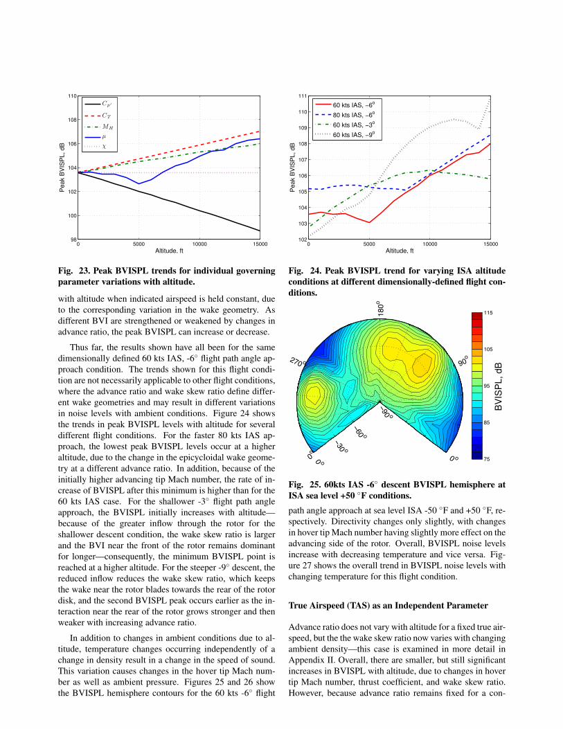
Fig. 23. Peak BVISPL trends for individual governingparameter variations with altitude.
with altitude when indicated airspeed is held constant, dueto the corresponding variation in the wake geometry. Asdifferent BVI are strengthened or weakened by changes inadvance ratio, the peak BVISPL can increase or decrease.
Thus far, the results shown have all been for the samedimensionally defined 60 kts IAS, -6# flight path angle ap-proach condition. The trends shown for this flight condi-tion are not necessarily applicable to other flight conditions,where the advance ratio and wake skew ratio define differ-ent wake geometries and may result in different variationsin noise levels with ambient conditions. Figure 24 showsthe trends in peak BVISPL levels with altitude for severaldifferent flight conditions. For the faster 80 kts IAS ap-proach, the lowest peak BVISPL levels occur at a higheraltitude, due to the change in the epicycloidal wake geome-try at a different advance ratio. In addition, because of theinitially higher advancing tip Mach number, the rate of in-crease of BVISPL after this minimum is higher than for the60 kts IAS case. For the shallower -3# flight path angleapproach, the BVISPL initially increases with altitude—because of the greater inflow through the rotor for theshallower descent condition, the wake skew ratio is largerand the BVI near the front of the rotor remains dominantfor longer—consequently, the minimum BVISPL point isreached at a higher altitude. For the steeper -9# descent, thereduced inflow reduces the wake skew ratio, which keepsthe wake near the rotor blades towards the rear of the rotordisk, and the second BVISPL peak occurs earlier as the in-teraction near the rear of the rotor grows stronger and thenweaker with increasing advance ratio.
In addition to changes in ambient conditions due to al-titude, temperature changes occurring independently of achange in density result in a change in the speed of sound.This variation causes changes in the hover tip Mach num-ber as well as ambient pressure. Figures 25 and 26 showthe BVISPL hemisphere contours for the 60 kts -6# flight
0 5000 10000 15000102
103
104
105
106
107
108
109
110
111
Altitude, ft
Pe
ak B
VIS
PL
, d
B
60 kts IAS, !6o
80 kts IAS, !6o
60 kts IAS, !3o
60 kts IAS, !9o
Fig. 24. Peak BVISPL trend for varying ISA altitudeconditions at different dimensionally-defined flight con-ditions.
!"#
$"#
%"#
&'"
&&"
###'(
#)!' (
#&$'(
##%'(
###' (
##!%' (
##!*' (##!
+' (
####' (
BV
ISP
L,dB
Fig. 25. 60kts IAS -6# descent BVISPL hemisphere atISA sea level +50 #F conditions.path angle approach at sea level ISA -50 #F and +50 #F, re-spectively. Directivity changes only slightly, with changesin hover tip Mach number having slightly more effect on theadvancing side of the rotor. Overall, BVISPL noise levelsincrease with decreasing temperature and vice versa. Fig-ure 27 shows the overall trend in BVISPL noise levels withchanging temperature for this flight condition.
True Airspeed (TAS) as an Independent Parameter
Advance ratio does not vary with altitude for a fixed true air-speed, but the the wake skew ratio now varies with changingambient density—this case is examined in more detail inAppendix II. Overall, there are smaller, but still significantincreases in BVISPL with altitude, due to changes in hovertip Mach number, thrust coefficient, and wake skew ratio.However, because advance ratio remains fixed for a con-

!"#
$"#
%"#
&'"
&&"
###'(
#)!' (#&$'(
##%'(
###' (
##!%' (
##!*' (##!
+' (
####' (
BV
ISP
L,dB
Fig. 26. 60kts IAS -6# descent BVISPL hemisphere atISA sea level -50 #F conditions.
!50 !40 !30 !20 !10 0 10 20 30 40 5092
94
96
98
100
102
104
106
108
110
112
! ISA Sea Level Temperature, oF
Pe
ak
BV
ISP
L,
dB
PeakAverage
Fig. 27. Variation of BVISPL values for ISA sea leveltemperature variations at 60 kts IAS, -6# descent flight.
stant true airspeed, the directivity of the BVI is not changedsignificantly. There is a moderate increase in thicknessnoise levels with altitude for high true airspeed flight condi-tions and a moderate decrease in levels with altitude for lowtrue airspeed flight conditions. This is because thicknessnoise is more sensitive to changes in the speed of sound athigher advancing tip Mach numbers.
Implications for Mission Planning Tools
The implications for the development of land-use and mis-sion planning tools are clear; helicopter source noise mod-els must incorporate the effects of ambient conditions onthe rotor noise sources in order to avoid significant errors inthe estimation of ground noise and detectability contours.The effects of ambient condition variations are somewhatdifferent for each rotor harmonic noise source; if correc-tions for ambient conditions are to be developed for empir-
ical helicopter source noise modeling methods, the effectson each noise source on the overall external noise radiationneed to be considered separately. For this reason, no simpleapproach is likely to provide an accurate and complete cor-rection of existing helicopter noise source models. Currentempirical helicopter noise source models generally classifyflight conditions in terms of indicated airspeed and flightpath angle—under a single known ambient condition, thiscorresponds to variations in advance ratio and wake skewratio. Variations in hover tip Mach numbers and thrust coef-ficients captured during typical test programs are small andunintentional, but variations in these parameters can be sig-nificant over the practical range of helicopter operating con-ditions. The physics-based and non-dimensional FRAMEmethod offers one solution to this problem, allowing rotornoise models to be constructed for each noise source us-ing both measured flight test data of a full scale vehicleunder a practical range of operating conditions and windtunnel data of similar rotors under a much wider and morecarefully controlled range of operating conditions than canbe achieved in flight. However, the FRAME method willrequire validation against measurements of full scale heli-copters operating across a range of ambient conditions be-fore it is ready for routine use.
Conclusions
The parameters that govern helicopter external harmonicnoise radiation have been analyzed using a non-dimensionalform of semi-empirical theory and parameter identificationtechniques. Although the approach was applied to the Bell206B3 two-bladed helicopter in this paper, the findings arethought to be representative of other single main rotor he-licopters. Based upon this modeling, the noise producedby a helicopter operating at several different altitudes wasestimated. Based upon these results, it was found that:
• In hover, lower frequency noise due to steady loadingincreases slightly with altitude. Decreases in ambientpressure with altitude reduce the radiated noise but aremitigated by increasing hover Mach numbers. In for-ward flight, the lower harmonics of loading will con-tribute as well and noise will also vary with advanceratio.
• Thickness noise levels increase with increasing alti-tude when flying constant indicated airspeed becauseof the dependency of thickness noise on advancingtip Mach number. It is mitigated slightly because ofdecreasing atmospheric pressures, but the strong de-pendency on advancing tip Mach number dominates(8 dB OASPL/10,000 ft). In practice, increases in ad-vancing tip Mach number may cause HSI noise to de-velop at altitude, leading to further increases in noiselevels and changes in the frequency spectrum of radi-ated noise.

• When flying true airspeed, the change in thicknessnoise levels with increasing altitude is more mod-erate. The increase in hover tip Mach number in-creases thickness noise levels, but is counteracted bythe decrease in ambient pressure. At high true air-speeds, the net effect is an increase in thickness noise(3/4 dB OASPL/10,000 ft at 100 kts TAS), but atlow airspeeds, thickness noise decreases with altitude(-1 dB OASPL/10,000 ft at 60 kts TAS).
• BVI noise can change markedly with altitude for flightoperations at constant indicated airspeed. Indicatedairspeed compensates for decreasing density at alti-tude by increasing the forward airspeed of the heli-copter. This changes the helicopters true airspeed,which changes the epicycloidal BVI intersection pat-terns, thus changing the directivity and magnitude ofthe resulting noise. The decrease in air density withaltitude also increases the circulation strength of thetip vortices trailed from each blade, causing increasesin BVI noise levels. In addition, decreasing tempera-ture with altitude increases BVI noise radiation levelsdue to increasing Mach numbers. Changes of up to7 dB BVISPL per 10,000 feet altitude were estimated.
• Flying true airspeed tends to maintain BVI noiseradiation patterns and noise levels. Advance ratiois constant with altitude explaining the similarity ofthe radiation patterns. Noise levels increase slightly(1 dB BVISPL/10,000 ft) with altitude because of in-creasing tip vortex strength and increasing Mach num-bers, but the increase is mitigated to some degree bythe decrease in atmospheric pressure.
• Formulating the problem in non-dimensional termsis helpful in interpreting the variations in the acous-tic state of the rotor with variation in the operatingcondition. The sensitivity of the radiated noise eachnon-dimensional governing parameter has been clearlyshown.
These results show that it is important to consider how mea-sured helicopter acoustic data taken under a given set ofconditions might be used to predict noise under differentoperational conditions. It is obvious that Mach number is animportant parameter that will strongly govern radiated noiseand should be carefully accounted for. For BVI noise, if thehelicopter is flown so that true airspeed (TAS) is constant,then the measured noise patterns that have been gatheredat one altitude can approximate the noise that is radiated atother altitudes. However, if indicated airspeed (IAS) is heldat these different altitudes, then significant changes in thepatterns and levels of BVI noise are to be expected.
Appendix I: Non-Dimensionalization and Developmentof the Governing Parameters of Rotor Harmonic Noise
Non-Dimensionalization
In most cases, physical relationships among variablescan be discovered by formulating problems using non-dimensional analysis. Buckingham’s # theorem, formal-ized one century ago, provides a systematic procedure fordetermining a set of non-dimensional parameters governinga physical process. When a problem is correctly formulatedon a non-dimensional basis, key relationships between thevariables become defined in a way which makes their phys-ical significance more clear.
Consider the Ffowcs Williams – Hawkings (Ref. 23)equation, Eq. 1, which describes the sound generated byarbitrary surfaces in motion:
p"(x, t) =1
4*++ t
!
S
"%0vn
r |1$Mr|
#
'dS $ (monopole) (1)
14*
++xi
!
S
"Pi jn j
r |1$Mr|
#
'dS + (dipole)
14*
+ 2
+xix j
!
S
"Qi j
r |1$Mr|
#
'dS (quadrupole)
The monopole term models thickness noise by consider-ing the rotor blade as a set of monopole mass sources andsinks which describe how the blades displace the medium.The dipole term models the mechanisms of loading noise,including BVI, as a set of aerodynamic dipole sources onthe surface of the blades that describe the forces the bladesexert on the medium. The quadrupole term includes the ef-fects of complex noise sources inside a fluid volume sur-rounding the rotor blades—this is how the effect of thetransonic flow field that causes HSI noise is modeled. Inthis paper, the quadrupole term is neglected and the mod-eling restricted to lower tip Mach number operating condi-tions where HSI noise does not occur. The FW-H equa-tion for the monopole and dipole terms can be rewrittenin non-dimensional form (Eq. 2), following the approachof Reference 13, where all all geometric terms are non-dimensionalized by the rotor radius, and all temporal termsby the rotor rotational rate.
Cp"(x, t) =1
4*++ t
!
S
$ Mr(1$Mr)
dS$ (2)
14*
++ xi
!
S
Cpi j n jM2
r(1$Mr)dS
where the acoustic pressure has been non-dimensionalizedwith respect to the ambient pressure (expressed as a func-tion of ambient density and speed of sound):
Cp"(x, t) =p"(x, t)%0a2
0(3)

and the blade surface pressures are non-dimensionalized bythe dynamic pressure at the respective blade element:
Cpi j =pi j
%0U2(r,))(4)
This non-dimensionalization indicates that for an other-wise identical non-dimensional operating condition of therotor, the acoustic pressure amplitudes will vary in propor-tion to the ambient pressure ratio, as expressed in Eq. 5.
p"1(x, t) =(%0a2
0)1
(%0a20)2
p"2(x, t) (5)
Governing Parameters of Rotor Harmonic Noise
The non-dimensional rotor operating condition is definedby a set of four independent parameters which are known(Refs. 13, 24) to govern the rotor harmonic noise sources,and these parameters can be expressed as the wake skew ra-tio ((), advance ratio (µ), thrust coefficient (CT ), and hovertip Mach number (MH ). This set of four non-dimensionalgoverning parameters is derived from the physical pro-cesses of rotor harmonic noise generation, including thick-ness and BVI noise.
For a fixed hover tip speed, hover tip Mach number isdefined by the ambient speed of sound:
MH ="Ra0
(6)
where ambient speed of sound can be estimated in air witha function of ambient temperature:
a0 =$
"!R!T0 (7)
Likewise, the rotor advance ratio is determined by thetrue airspeed at which the rotor moves through the medium.
µ =V
"R(8)
This can be related to the indicated airspeed, which isa function of dynamic pressure, through air density usingthe following expression valid for the range of rotorcraftairspeeds and altitudes:
VIAS =V%
%0
%SL(9)
The combination of hover tip Mach number and advanceratio therefore specify the Mach number of all blade sec-tions at all azimuths.
M = M(r,)) = MH(r+µ sin)) (10)
For example, equation 10 can be used to relate the hoverand advancing tip Mach numbers:
MAT = MH (1+µ) (11)
The advance ratio and hover tip Mach number also setthe epicycloidal pattern of the wake formed by the trailedtip vortices responsible for BVI, as shown in Figure 28. Incombination, these two governing parameters set the num-ber of potential BVI occurring on the advancing and retreat-ing sides of the rotor, as well as the interaction angles be-tween the rotor blades and the vortices during BVI events.The interaction angle of BVI controls how the acoustic dis-turbance accumulates in phase through the medium, andtherefore contributes to the amplitude of BVI impulses anddetermines the azimuthal directivity of BVI noise. Figures29 and 30 use 2D Huygens’ wavelets to illustrate how theBVI phasing process causes the radiation of noise towardsspecific azimuths for oblique and parallel BVI, respectively.
The thrust coefficient is the non-dimensionalization ofrotor thrust with respect to a reference dynamic pressure,calculated from the rotor tip speed and ambient air density,and a reference area taken as the rotor disk area.
CT =T
%0 A("R)2 (12)
For steady flight conditions, the rotor thrust is approx-imately equal to the vehicle weight. Therefore, the ambi-ent air density determines thrust coefficient for a particu-lar rotorcraft with fixed gross weight and rotor tip speed.The thrust coefficient relates to the blade section loading,and hence influences lower harmonic loading noise. In ad-dition, the trailed tip vortex circulation strength is directlyproportional to rotor thrust coefficient, which influences thestrength and acoustic impact of BVI events. For instance,the analytical solution for the non-dimensionalized trailedtip vortex circulation strength due to an idealized triangularspanwise lift distribution is shown in Eq. 13.
!"R2 =
2*CT
b(13)
The thrust coefficient is also directly related to the bladeloading coefficient, CT/& , which has a similar form to thenon-dimensionalized blade surface pressure term, Cpi j , ofEquation 2. Through Equation 14, provided in Reference26, the blade loading coefficient can also be related to themean lift coefficient of the rotor blade sections. In hoveringflight, rotor stall occurs for CT/& % 0.13, and decreaseswith increasing advance ratio due to asymmetry in local liftcoefficient. Consequently, as altitude increases so does theblade loading coefficient, bringing the rotor closer to stall.Not only does this impose limits on the operation of thehelicopter in high altitude conditions, it will also changerotor’s aerodynamic and acoustic state.
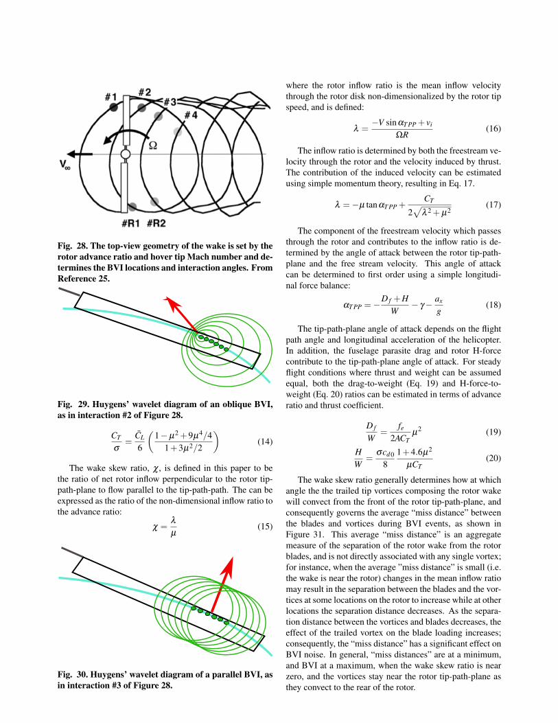
Fig. 28. The top-view geometry of the wake is set by therotor advance ratio and hover tip Mach number and de-termines the BVI locations and interaction angles. FromReference 25.
Fig. 29. Huygens’ wavelet diagram of an oblique BVI,as in interaction #2 of Figure 28.
CT
&=
CL
6
&1$µ2 +9µ4/4
1+3µ2/2
'(14)
The wake skew ratio, ( , is defined in this paper to bethe ratio of net rotor inflow perpendicular to the rotor tip-path-plane to flow parallel to the tip-path-path. The can beexpressed as the ratio of the non-dimensional inflow ratio tothe advance ratio:
( =#µ
(15)
Fig. 30. Huygens’ wavelet diagram of a parallel BVI, asin interaction #3 of Figure 28.
where the rotor inflow ratio is the mean inflow velocitythrough the rotor disk non-dimensionalized by the rotor tipspeed, and is defined:
# =$V sin!T PP + vi
"R(16)
The inflow ratio is determined by both the freestream ve-locity through the rotor and the velocity induced by thrust.The contribution of the induced velocity can be estimatedusing simple momentum theory, resulting in Eq. 17.
# =$µ tan!T PP +CT
2$
# 2 +µ2(17)
The component of the freestream velocity which passesthrough the rotor and contributes to the inflow ratio is de-termined by the angle of attack between the rotor tip-path-plane and the free stream velocity. This angle of attackcan be determined to first order using a simple longitudi-nal force balance:
!T PP =$D f +H
W$ " $ ax
g(18)
The tip-path-plane angle of attack depends on the flightpath angle and longitudinal acceleration of the helicopter.In addition, the fuselage parasite drag and rotor H-forcecontribute to the tip-path-plane angle of attack. For steadyflight conditions where thrust and weight can be assumedequal, both the drag-to-weight (Eq. 19) and H-force-to-weight (Eq. 20) ratios can be estimated in terms of advanceratio and thrust coefficient.
D f
W=
fe
2ACTµ2 (19)
HW
=&cd0
81+4.6µ2
µCT(20)
The wake skew ratio generally determines how at whichangle the the trailed tip vortices composing the rotor wakewill convect from the front of the rotor tip-path-plane, andconsequently governs the average “miss distance” betweenthe blades and vortices during BVI events, as shown inFigure 31. This average “miss distance” is an aggregatemeasure of the separation of the rotor wake from the rotorblades, and is not directly associated with any single vortex;for instance, when the average ”miss distance” is small (i.e.the wake is near the rotor) changes in the mean inflow ratiomay result in the separation between the blades and the vor-tices at some locations on the rotor to increase while at otherlocations the separation distance decreases. As the separa-tion distance between the vortices and blades decreases, theeffect of the trailed vortex on the blade loading increases;consequently, the “miss distance” has a significant effect onBVI noise. In general, “miss distances” are at a minimum,and BVI at a maximum, when the wake skew ratio is nearzero, and the vortices stay near the rotor tip-path-plane asthey convect to the rear of the rotor.

Fig. 31. The side-view geometry of the wake is set bythe rotor inflow and determines the “miss-distance” be-tween the vorticies and blades during BVI. From Refer-ence 25.
Appendix II: Flight ConditionsDefined by True Airspeed
While flight conditions are typically defined in terms of in-dicated airspeed (IAS), which varies with dynamic pres-sure, another option is to define flight conditions with re-spect to true air speed (TAS). Figure 32 shows the varia-tion in non-dimensional governing parameter values withchanging ISA altitude conditions for the case where trueairspeed is held constant, similar to Figure 1 for the typicalindicated airspeed case. In this situation, the advance ra-tio does not vary, such that the freestream dynamic pressuredecreases with altitude. This leads to a decreasing fuselageparasite drag and rotor H-force, causing the rotor tip-path-plane to tilt backwards and reducing the inflow through therotor. On the other hand, the reduction in air density leadsto a substantial increase in induced inflow—overall, there isa greater increase in inflow for constant true airspeed (TAS)than when flying constant indicated airspeed (IAS). Sinceinflow increases relative to the constant true airspeed, thewake skew ratio varies with altitude. This results in the de-scent angle required for zero wake skew (and hence nearmaximum BVI noise) varying with altitude, as shown inFigure 33. Depending on the true airspeed flow, the sensi-tivity of BVI to flight condition will change. The BVISPLhemisphere contours for a 60 kts TAS -6# flight path angleapproach condition at ISA altitudes of 5,000, 10,000 and15,000 ft are shown in Figures 34, 35 and 36, respectively.The retreating side BVI “hotspot” location remains fixedwith altitude, since advance ratio remains unchanged. Theincrease in the wake skew ratio causes a small increase inthe “miss-distances” of the BVI, but this is mitigated by theincrease in thrust coefficient and Mach numbers with alti-tude. The overall increase in BVISPL with altitude is shownin Figure 37. In general, the changes in BVISPL magnitude
0 5000 10000 1500080
100
120
140
160
Altitude above MSL, ft
Perc
en
t o
f M
SL
Valu
e
µ!
0 5000 10000 1500080
100
120
140
160
Altitude above MSL, ft
Perc
en
t o
f M
SL
Valu
e
CTMH
Fig. 32. The relative variation in non-dimensional gov-erning parameters with ISA altitude for a Bell 206B3 in60 kts TAS -6.0# descending flight.
30 40 50 60 70 80 90 100!15
!10
!5
0F
light P
ath
Angle
(!),
degre
es
True Airspeed, kts
Sea Level10,000 ft20,000 ft
Fig. 33. A plot of the dimensionally-defined zero wakeskew ratio flight conditions at various altitudes.
and directivity with changing ambient conditions are some-what less pronounced and are more predictable when defin-ing flight conditions by true airspeed instead of indicatedairspeed, because the advance ratio remains fixed.
The variation in thickness noise with altitude is likewisedifferent for flight conditions defined by true airspeed thanfor those defined by indicated airspeed. Since advance ra-tio remains fixed, the advancing tip Mach number only in-creases in proportion to the increase in hover tip Mach num-ber with altitude. In addition, the reduction in ambient pres-sure with altitude reduces the amplitude of thickness noise.Figure 38 plots the peak thickness noise level variation withaltitude in OASPL for several different true airspeeds. De-pending on the true airspeed of the vehicle, thickness noisemay either increase or decrease with increasing altitude.Higher true airspeeds correspond to higher advancing tipMach numbers, where the thickness noise is more sensitiveto further increases in advancing tip Mach number due to

!"#
$"#
%"#
&'"
&&"
###'(
#)!' (#&$'(
##%'(
###' (
##!%' (
##!*' (##!
+' (
####' (
BV
ISP
L,dB
Fig. 34. 60kts TAS -6# descent BVISPL hemisphere atISA 5,000 ft conditions.(µ = 0.14 , ( = 0.048 ,CT = 0.0034 , MH = 0.67)
the decrease in ambient temperature. In practice, further in-creases in advancing tip Mach number at high flight speedsmay yield even higher increases in noise than predicted aslocal transonic flow allows HSI noise to develop.
In practice, helicopters must be flown according to theindicated airspeed, because the aerodynamic forces andhence vehicle performance parameters are tied to the dy-namic pressure, which varies with air density. However,so long as vehicle performance at altitude is taken intoaccount when designing helicopter trajectories, helicopternoise modeling might be conducted more accurately onthe basis of flight conditions defined by true airspeed thanon the basis of indicated airspeed; in conjunction with theflight path angle, this is equivalent to specifying flight con-ditions on a non-dimensional basis of advance ratio and
!"#
$"#
%"#
&'"
&&"
###'(
#)!' (
#&$'(
##%'(
###' (
##!%' (
##!*' (##!
+' (
####' (
BV
ISP
L,dB
Fig. 35. 60kts TAS -6# descent BVISPL hemisphere atISA 10,000 ft conditions.(µ = 0.14 , ( = 0.054 ,CT = 0.0039 , MH = 0.68)
!"#
$"#
%"#
&'"
&&"
###'(
#)!' (
#&$'(
##%'(
###' (
##!%' (
##!*' (##!
+' (
####' (
BV
ISP
L,dB
Fig. 36. 60kts TAS -6# descent BVISPL hemisphere atISA 15,000 ft conditions.(µ = 0.14 , ( = 0.064 ,CT = 0.0046 , MH = 0.70)
0 5000 10000 15000 2000092
94
96
98
100
102
104
106
108
110
112
Altitude, ft
Pe
ak
BV
ISP
L,
dB
PeakAverage
Fig. 37. Variation of BVISPL values for ISA altitudeconditions at 60 kts TAS, -6# descent flight.
wake skew ratio for steady flight conditions. Due to thestrong effect of advance ratio on rotor harmonic noise, itis also cautioned that flight conditions should not be de-fined on the basis of ground speed in helicopter source noisemodels, since ground speed is not equivalent to true air-speed except in the absence of wind.
Acknowledgements
The authors would like to thank Dr. Ben Wel-C Sim andMichael E. Watts for helpful discussions during the prepa-ration of this paper. In addition, the authors would like tothank Richard D. Sickenberger, David A. Conner, CharlesD. Smith, Ernesto Moralez, and William A. Decker for theirimportant roles in the 2006 flight test of the Bell 206B3 he-licopter at Moffett Field, CA.

0 5000 10000 15000100
101
102
103
104
105
106
107
108
109
110
Altitude, ft
OA
SP
L,
dB
100 kts TAS
80 kts TAS
60 kts TAS
Fig. 38. Peak OASPL thickness noise level variation forISA altitude conditions for constant TAS flight.
References
1Fleming, G. G. and Rickley, E. J., “Heliport NoiseModel, HNM. Version 2.2 (User’s Guide),” Technical re-port, Federal Aviation Administration, February 1994.
2Connor, T. L., “Integrated Noise Model-The FederalAviation Administration’s computer program for predictingnoise exposure around an airport,” Inter-noise 80: Noisecontrol for the 80’s, Jan 1980.
3Lucas, M. J. and Marcolini, M. A., “Rotorcraft NoiseModel,” AHS Technical Specialists’ Meeting for RotorcraftAcoustics and Aerodynamics, October 1997.
4Conner, D. A. and Page, J. A., “A Tool for Low NoiseProcedures Design and Community Noise Impact Assess-ment: The Rotorcraft Noise Model (RNM),” Heli Japan,2002.
5Browne, R. W., Munt, R. M., Simpson, C. R., andWilliams, T., “Prediction of Helicopter Noise Contoursfor Land Use Planning,” 10th AIAA/CEAS AeroacousticsConference, 2004.
6Gervais, M., Gareton, V., Dummel, A., and Heger, R.,“Validation of EC130 and EC135 Environmental ImpactAssessment using HELENA,” American Helicopter Society66th Annual Forum, May 2010.
7Guntzer, F., Spiegel, P., and Lummer, M., “Genetic Op-timizations of EC-135 Noise Abatement Flight Proceduresusing and Aeroacoustic Database,” 35th European Rotor-craft Forum, September 2009.
8Fleming, G. G., Plotkin, K. J., Roof, C. J., Ikelheimer,B. J., and Senzig, D. A., “Assessment of Tools for Model-ing Aircraft Noise in the National Parks,” Technical report,FICAN, March 2005.
9International Organization for Standardization, “Stan-dard Atmosphere,” Technical Report 2533:1975, ISO,1975.
10Greenwood, E. and Schmitz, F. H., “A Parameter Identi-fication Method for Helicopter Noise Source Identificationand Physics-Based Semi-Empirical Modeling,” AmericanHelicopter Society 66th Annual Forum, May 2010.
11Greenwood, E. and Schmitz, F. H., “Separation of Mainand Tail Rotor noise Ground-Based Acoustic Measure-ments using Time-Domain De-Dopplerization,” 35th Euro-pean Rotorcraft Forum, September 2009.
12Schmitz, F. H., Greenwood, E., Sickenberger, R. D.,Gopalan, G., Sim, B. W.-C., Conner, D. A., Moralez, E.,and Decker, W., “Measurement and Characterization of He-licopter Noise in Steady-State and Maneuvering Flight,”American Helicopter Society 63rd Annual Forum, May2007.
13Schmitz, F. H., Boxwell, D. A., Lewy, S., and Dahan, C.,“Model- to Full-Scale Comparisons of Helicopter Blade-Vortex Interaction Noise,” Journal of the American Heli-copter Society, Vol. 29, (2), 1984, pp. 16–25.doi: 10.4050/JAHS.29.16
14Farassat, F., “Derivation of Formulations 1 and 1Aof Farassat,” Technical Report TM-2007-214853, NASA,2007.
15Beddoes, T. S., “A wake model for high resolution air-loads,” International Conference on Rotorcraft Basic Re-search, February 1985.
16van der Wall, B. G., “The Effect of HHC on the VortexConvection in the Wake of a Helicopter Rotor,” AerospaceScience and Technology, Vol. 4, (5), 2000, pp. 321–336.
17Bhagwat, M. J. and Leishman, J. G., “Generalized Vis-cous Vortex Core Models for Application to Free-VortexWake and Aeroacoustic Calculations,” 58th Annual Forumof the American Helicopter Society, June 2002.
18Landgrebe, A. J., “The wake geometry of a hovering he-licopter rotor and its influence on rotor performance,” Jour-nal of the American Helicopter Society, Vol. 17, (4), 1972.
19Beddoes, T. S., “Practical Computation of UnsteadyLift,” Vertica, Vol. 8, (1), 1984.
20Leishman, J. G., Principles of Helicopter Aerodynam-ics, Cambridge University Press, New York, second edition,2006.
21Schmitz, F. H. and Sim, B. W.-C., “Radiation and Direc-tionality Characteristics of Helicopter Blade-Vortex Inter-action Noise,” Journal of the American Helicopter Society,Vol. 48, (4), 2003, pp. 253–269.

22Snyder, J. P., “Map Projections: A Working Manual,”Technical Report PP1395, USGS, 1982.
23Ffowcs Williams, J. E. and Hawkings, D. L., “Soundgeneration by turbulence and surfaces in arbitrary motion,”Transactions for the Royal Society of London, Vol. 264,May 1969, pp. 321–342.
24Schmitz, F. H. and Sim, B. W.-C., “Acoustic Phasing, Di-rectionality and Amplification Effects of Helicopter Blade-Vortex Interactions,” Journal of the American HelicopterSociety, Vol. 46, (4), 2001, pp. 273–282.doi: 10.4050/JAHS.46.273
25Schmitz, F. H., “Rotor Noise,” Aeroacoustics of FlightVehicles: Theory and Practice, edited by H. H. Hubbard,Vol. 1, Acoustical Society of America, first edition, 1995,pp. 65–145.
26Harris, F. D., “Rotary Wing Aerodynamics—HistoricalPerspective and Important Issues,” AHS Technical Special-ists’ Meeting on Aerodynamics and Aeroacoustics, Febru-ary 1987.