construction of a four rotor helicopter control systemetd.dtu.dk/thesis/243342/thesis_dagur.pdf ·...
TRANSCRIPT

Thorhallur Tomas BuchholzDagur Gretarsson
Construction of a Four RotorHelicopter Control System
Master’s Thesis, February 2009


Thorhallur Tomas BuchholzDagur Gretarsson
Construction of a Four RotorHelicopter Control System
Master’s Thesis, February 2009


Construction of a Four Rotor Helicopter Control System,
This report was prepared byThorhallur Tomas BuchholzDagur Gretarsson
SupervisorsElbert Hendricks
Release date: Date publishedCategory: 1 (public)
Edition: First
Comments: This report is part of the requirements to achieve the Master ofScience in Engineering (M.Sc.Eng.) at the Technical Universityof Denmark. This report represents 30 ECTS points.
Rights: c©Dagur Gretarsson and Thorhallur Tomas Buchholz, 2009
Department of Electrical EngineeringAutomation (AU)Technical University of DenmarkElektrovej building 326DK-2800 Kgs. LyngbyDenmark
www.elektro.dtu.dk/forskning/auTel: (+45) 45 25 35 50Fax: (+45) 45 88 12 95E-mail: [email protected]


Construction of a Four RotorHelicopter Control System
Thorhallur Tomas BuchholzDagur Gretarsson
Master’s Thesis, February 2009

Abstract
This report presents the construction of a four rotor helicopter control sys-tem.
A nonlinear dynamic model of a custom built four rotor helicopter is pre-sented. This model is linearized in order to serve as basis for the design ofa LQ regulator. The LQ regulator is realized using a microprocessor basedflight controller mounted on the custom built four rotor helicopter. Theflight controller runs a flight routine designed to work as a stability aug-mented control system for a pilot.
Flight tests suggest that the stabilizing LQ regulator works properly. Thenonlinear model has also been partly validated, but further improvementsof the code for the flight controller are needed in order to confirm this indetail.


Dansk Resume
Denne rapport præsenterer konstruktion af et fire rotor helikopter kontrolsystem.
En ulineær dynamisk model, af en specialfremstillet fire rotor helikopter,bliver præsenteret. Denne model bliver lineariseret for at danne grundlagfor designet af en LQ regulator. LQ regulatoren bliver realiseret ved brugaf et mikrokontroller baseret fly styresystem monteret pa den specialfrem-stillede fire rotor helikopter. Fly styresystemet eksikverer en fly rutine somer designet til at virke som stabilitets supplerende reguleringssystem for enpilot.
Fly tests tyder pa at den stabiliserende LQ regulator virker rigtigt. Denulineære model er ogsa delvis blevet valideret, men yderligere forbedringerpa fly kontrollerens kode er nødvendige for at konstatere dette.


Acknowledgments
We wish first and foremost to thank our supervisor Elbert Hendricks for hispatience, guidance and support. We also like to think Bertil Morelli for hishelp with the construction of the helicopter and those who supported us invarious ways during the project. We finally wish to thank Free2move fortheir generous contribution in form of the Bluetooth module.

Contents
Nomenclature xi
1 Introduction 1
2 Four rotor principles 5
2.1 Single rotor helicopter . . . . . . . . . . . . . . . . . . . . . . 5
2.2 Four rotor helicopter . . . . . . . . . . . . . . . . . . . . . . . 8
3 Four rotor helicopter platform 11
4 Four rotor dynamics 15
4.1 Attitude representation . . . . . . . . . . . . . . . . . . . . . 16
4.2 Nonlinear equations of motion . . . . . . . . . . . . . . . . . . 17
4.2.1 Forces acting on the helicopter . . . . . . . . . . . . . 20
4.2.2 Torques acting on the helicopter . . . . . . . . . . . . 22
4.3 Simulink models . . . . . . . . . . . . . . . . . . . . . . . . . 24
4.3.1 Model in reference frame . . . . . . . . . . . . . . . . 25
4.3.2 Model in body frame . . . . . . . . . . . . . . . . . . . 25
4.4 Linearized models . . . . . . . . . . . . . . . . . . . . . . . . 26
4.4.1 Linearized model in reference frame . . . . . . . . . . 27
4.4.2 Linearized model in body frame . . . . . . . . . . . . . 29

4.5 Open loop simulations of model in body frame . . . . . . . . 30
4.6 Motor model . . . . . . . . . . . . . . . . . . . . . . . . . . . 31
5 Controller design 35
5.1 Linear Quadratic Regulator . . . . . . . . . . . . . . . . . . . 35
5.2 Designing a continuous LQR for attitude and position stabi-lization . . . . . . . . . . . . . . . . . . . . . . . . . . . . . . 38
5.3 Designing a reduced continuous LQR for attitude stabilization 45
5.4 Discrete Linear Quadratic Regulator . . . . . . . . . . . . . . 48
5.5 Designing a discrete LQR . . . . . . . . . . . . . . . . . . . . 48
6 Hardware 53
6.1 The flight controller . . . . . . . . . . . . . . . . . . . . . . . 53
6.2 The microprocessor . . . . . . . . . . . . . . . . . . . . . . . . 54
6.3 Blutooth module . . . . . . . . . . . . . . . . . . . . . . . . . 55
6.4 Motors . . . . . . . . . . . . . . . . . . . . . . . . . . . . . . . 57
6.5 Sensors . . . . . . . . . . . . . . . . . . . . . . . . . . . . . . 59
6.6 Print Circuit Board . . . . . . . . . . . . . . . . . . . . . . . 60
6.7 Receiver . . . . . . . . . . . . . . . . . . . . . . . . . . . . . . 61
7 Software structure 63
7.1 Code flow diagrams . . . . . . . . . . . . . . . . . . . . . . . . 63
7.2 Code performance . . . . . . . . . . . . . . . . . . . . . . . . 70
8 Flight test and model validation 73
9 Conclusion 81
9.1 Conclusion on the helicopter construction . . . . . . . . . . . 81
9.2 Conclusion on the controller design and simulations . . . . . . 82
9.3 Conclusion on the validation of the nonlinear dynamic model 83
References 84

Appendix 88
A Rotating frame of reference 89
B Equations of angular motion 93
B.1 Torque . . . . . . . . . . . . . . . . . . . . . . . . . . . . . . . 93
B.2 Inertia tensor . . . . . . . . . . . . . . . . . . . . . . . . . . . 95
C Euler angle rotation 99
D Thrust and H-force 101
D.1 Rotor thrust . . . . . . . . . . . . . . . . . . . . . . . . . . . . 101
D.2 H-force . . . . . . . . . . . . . . . . . . . . . . . . . . . . . . . 102
E The inertia of the helicopter 103
F Rotor inertia 107
G Helicopter frame construction 111
G.1 Frame materials . . . . . . . . . . . . . . . . . . . . . . . . . . 111
G.2 Frame design . . . . . . . . . . . . . . . . . . . . . . . . . . . 113
G.2.1 Frame arms . . . . . . . . . . . . . . . . . . . . . . . . 113
G.2.2 Center cross . . . . . . . . . . . . . . . . . . . . . . . . 116
G.2.3 Center plates . . . . . . . . . . . . . . . . . . . . . . . 117
G.2.4 Rotor mountings . . . . . . . . . . . . . . . . . . . . . 118
G.2.5 Frame extra supports . . . . . . . . . . . . . . . . . . 118
G.3 Landing frame . . . . . . . . . . . . . . . . . . . . . . . . . . 119
G.4 The helicopter frame . . . . . . . . . . . . . . . . . . . . . . . 119
G.5 Frame drag . . . . . . . . . . . . . . . . . . . . . . . . . . . . 119
H The single chip yaw rate gyro ADXRS150 121
I Rotor measurements 127

x
I.1 Measurement setup . . . . . . . . . . . . . . . . . . . . . . . . 127
I.2 Applied rotor blades . . . . . . . . . . . . . . . . . . . . . . . 130
I.2.1 Duty cycle and angular velocity . . . . . . . . . . . . . 130
I.2.2 Angular velocity and thrust . . . . . . . . . . . . . . . 130
I.2.3 Angular velocity and torque . . . . . . . . . . . . . . . 132
I.3 Other rotor blades . . . . . . . . . . . . . . . . . . . . . . . . 133
I.3.1 Duty cycle versus angular velocity . . . . . . . . . . . 133
I.3.2 Angular velocity and thrust . . . . . . . . . . . . . . . 133
I.4 Figure of merit . . . . . . . . . . . . . . . . . . . . . . . . . . 134
J Momentum theory 137
K Level shifter simulation 145
L Schematics and PCB layouts 147
M Functions used in control loop 153

Nomenclature
x State derivatives vector 12x1, page 25
Γa Torque acceleration, page 24 Nm
Γf Torque flight, page 23 Nm
Γg Rotors gyro torque, page 23 Nm
Γr Torque rotor, page 23 Nm
Γx Torque about the x-a xis, page 23 Nm
Γx Torque about the x-axis, page 22 Nm
Γy Torque about the y-axis, page 22 Nm
Γ Torque in body frame Γ = [Γx,Γy,Γz]′, page 18 Nm
Ω Euler angular velocity in body frame Ω = [p, q, r]′, page 18 rads
a′ Acceleration in body frame a′ = [u, v, w]′, page 18 ms2
Aψθφ Attitude matrix, page 17
Fd Drag force, page 21 N
Fg Gravitation force, page 17 N
FH H-force, page 21 N
Fr Total rotor thrust, page 20 N
F Force in body frame F = [Fx, Fy , Fz]′, page 18 N
Iψθφ Inertia tensor, page 19 kgm2

xii
L0 Angular momentum in body frame L0 = [L,M,N ]′, page 18 kgm2
s
T1, T2, T3, T4 Thrust of the rotors, page 22 N
T Thrust vector, page 20 N
u Input vector 4x1, page 25 dutycycle
v Velocity in body frame v = [u, v,w]′, page 18 ms
x State vector 12x1, page 25
y Output vector 6x1, page 25
ω Rotor angular velocity, page 23 rads
ρ Air density, page 21 kgm3
Af Frontal area of the helicopter body, page 21 m2
Cf Drag coefficient, page 21 Ns2
kg
Ia Armature current, page 31 A
Ir Rotor moment of inertia, page 23 kgm2
Ixx Inertia about the bodys x-axis, page 19 kgm2
Iyy Inertia about the bodys y-axis, page 19 kgm2
Izz Inertia about the bodys z-axis, page 19 kgm2
Jm Motor moment of inertia, page 31 kgm2
Ke Back emf constant, page 31 V srad
Kt Motor moment constant, page 31 NmA
La Armature windings inductance, page 31 H
m Mass, page 18 kg
Mb Motor external load, page 31 Nm
Mf Motor friction, page 31 Nm
Mp Overshoot, page 41 %
Mu Motor torque, page 31 Nm
Ra Armature windings impedance, page 31 Ω
tr Rise time, page 41 s

xiii
ts Settling time, page 41 s
Va Armature voltage, page 31 V
Ve Back emf voltage, page 31 V

xiv

Chapter 1
Introduction
With the rapid development in microprocessor and sensor technology in theresent years, the interest for small four rotor helicopters has increased. Fourrotor helicopters have moved on from being an unattainable idea to becomepopular research objects within the realms of control theory, autonomousrobot theory, electronics and mechanics.
The particular interest of the research community in four rotor helicoptersas Unmanned Aerial Vehicles (UAV), can be explained by their advantagesover other equivalent vertical take of an landing UAV’s, such as single rotorhelicopters. In its simplicity, the four rotor helicopter does not need anycomplex mechanical controls of its rotors for vehicle control. Instead it usesrotor blades with fixed pitch and changes the angular velocity with the sameresults.
Its advantages become even more clear when it is used for indoor flight.As it uses four rotors to produce thrust, each rotor can be kept smaller indiameter relative to a single rotor helicopter, producing the same thrust.The moment of each rotor is subsequently much smaller and they are there-fore less harmful should they accidentally bumps into any objects.
This groups particular interest lies in the four rotor helicopter as a con-trol object. As such, it is a marginally stable multiple input multiple output(MIMO) system that has small time constants as a result of its small size.It is therefore considered to be a challenging project to design a controllerthat is able to stabilize the attitude of the helicopter while it is being flown

2 Introduction
by a pilot.
Many of the technical problems that limited earlier flight experiments withfour rotor helicopters are still valid in the present. In this report, this groupwill assess some of these problems and will seek to solve them in an accept-able manor. These are the following.
• The helicopter frame should be as stiff and strong as possible.
• The helicopters weight should be as low as possible for a prolongedflight time.
• The group has to understand and explain the basic aerodynamics thatare needed to make a stabilizing control system for the helicopter.
• The group has to provide stability and proper control to the helicopterfor an easy pilot augmented hover and forward flight.
To solve these problems, the group will design and custom build a four rotorhelicopter. This includes choosing suitable materials that will keep the he-licopter as strong and stiff as possible while being light weight at the sametime. Control electronics, rotors and batteries will also be chosen bearingthe weight in mind.
A linearized model of the helicopter will be made to serve as the basis for alinear controller design.
The stability control will be done with an on-board microprocessor runninga Linear Quadratic Regulator (LQR) as a attitude stabilizing augmentationfor a pilot controlled flight. The pilot will control the movements and posi-tion of the helicopter with a remote control.
A data link will be implemented on the helicopter in order to be able at-tain real time flight data for possible monitoring of the flight and analyticalpurposes.
Prior work on the subject
Many research groups are working on four rotor helicopters as UnmannedAerial Vehicle (UAV) testbeds for stabilizing control algorithms and sensing.Numerous UAV’s have seen success using Linearized Quad Regulator (LQR)derived from linearized dynamic models for attitude control.

3
The Stanford Testbed of Autonomous Rotorcraft for Multi-Agent Control(STARMAC) is an ongoing project that acts as a testbed for UAV’s. LQRcontrollers have been used successfully in providing attitude stabilization inthat project. During their work on this project, Hoffmann et al. (19) re-alized that by stiffening the helicopter frame greatly improved the attitudemeasurements of the inertial measuring unit (IMU). The frame was stiffenedby cross braces between the motors.
Nice (29) constructed a Autonomous Flying Vehicle (AFV). This four ro-tor helicopter project was based on a custom made airframe with brushlessmotors, for improved rotor efficiency, controlled by custom made electronicsto improve resolution. The attitude stabilization was done with a on-boardLQR controller based on a linearized model of the helicopter. A very stablehover flight was achieved with the aid of a human pilot correcting gyroscopicdrift.
Bertelsen et al. (4) constructed in the work on their masters thesis, a atti-tude stabilizing LQR on the bases of a proposed linearized model of a fourrotor helicopter. This controller was realized using a the frame includingrotors from a commercially available four rotor helicopter, the Draganflyer(11), and a xPC real time kernel to running the controller derived fromMatlab/Simulink. The measurements of angular velocity were provided bythree gyroscopes measuring Eulers angular velocities. The validation of themodel was made by comparing flight data with simulation data.

4 Introduction

Chapter 2
Four rotor principles
The principle of using four rotors to lift a helicopter from the ground is thetopic of this chapter. In order to emphasize the simplicity of the four rotorconcept and to familiarize the reader with helicopter principles in general,an introduction to a conventional single rotor helicopter will be presentedfirst.
2.1 Single rotor helicopter
All the lifting thrust of the single rotor helicopter is produced by the mainrotor, see figure 2.1. When the main rotor is rotating it has to overcomethe air resistance (drag) of the rotor blades. The torque that is applied tothe rotor shaft in order to overcome the drag is directly transmitted to thehelicopter body to which the rotor is attached.
It is customary to treat the rotor as if it had an infinite number of bladeswhich form a disc. This imaginary rotor disk, lies in the plane of the bladeswith the radius equal to the length of the blades. The thrust that the rotorproduces is always perpendicular to the rotor disc plane. When the heli-copter is in axial flight, that is flying up, down or hovering, the lift of therotor is symmetrical around the rotor’s axis.
One of the characteristic features of the single rotor helicopter is the tailrotor. The tail rotor’s thrust generates a torque which cancels out thetorque deriving from the main rotor as result of the blade drag. The pi-

6 Four rotor principles
lot also exploits the tail rotor to turn the helicopter body around the rotoraxis. This is done by changing the angular velocity of the tail rotor, andthereby its thrust. The tail rotor reacts immediately in a predefined way tothe pilots controls so that the pilot does not have to think about it when heis maneuvering the helicopter.
Figure 2.1: Single rotor helicopter. The tail rotor is used to produce anti-torqueto cancel out the torque generated by the main rotor when it is over-coming the rotor blade drag.(25, p. 57). The figure also shows thebasic rotational movements of the helicopter, roll, pitch and yaw.
Besides producing the lifting thrust, the main rotor is also the primary sourceof propulsion and control (25, p. 171). In forward flight, the main rotor diskis effectively tilted so that the otherwise vertical thrust in axial flight is nowtilted as well, see figure 2.2. The thrust in the figure is represented by twoforce components, the lifting force and the propulsion force. To maintainaltitude, the lifting force has to overcome the gravity force. The thrust musttherefore be increased when going from axial flight into forward flight in or-der to maintain the same altitude.
Tilting the rotor disk in the direction of choice is done by adjusting therotor blades. A rotor blade is generally attached to its hub by the means ofhinges located at the root of the blade, see figure 2.3. The hinges allow the

2.1 Single rotor helicopter 7
Figure 2.2: The two force components of the thrust when the rotor disk is tilted.
rotor blade to flap with respect to its hub plane (25, p. 172). Flapping isthe rotational motion of the blade about its flapping axis as shown in figure2.3. The possibility of pitching the rotor blades is also incorporated intothe blade design. Pitching is the rotation of the blade about its longitudinalaxis. Pitching the rotor blades collectively, that is all with the same angle,while maintaining constant rotor angular velocity changes the lift of the ro-tor. Changing the pitch of the rotor blades independently while they arerotating is called cyclic pitch. Cyclic pitch, which changes the distributionof forces over the rotor disk, is the key feature in tilting the rotor disk effec-tively in order to move the helicopter in axial flight.
Figure 2.3: Schematics of a rotor blade showing the basic movements of the rotorblade, flapping and pitch.
The mechanical complexity of controlling the blade movements mentionedabove causes stress on the rotor construction. This demands frequent main-tenance and component replacement in order to avoid rotor failure. It also

8 Four rotor principles
adds weight to the helicopter.
2.2 Four rotor helicopter
The four rotor helicopter concept is not new. In the year 1907 the firstreported successful helicopter flights with a helicopter, said to have lifted aman from the ground, were done by Paul Cornu of France (25, p. 11). Thesame year Breguet brothers made a quadrotor helicopter called GyroplaneNo. 1. This four rotor helicopter is said to have briefly lifted a man from theground into free flight. Leishman (25, p. 12) speculates that this flight waseven closer to being a real flight than that of Paul Cornu. The four rotorconcept does not seem to have been a success though, probably because it isbeyond the skills of even a trained pilot to fly the helicopter by controllingthe four rotors simultaneously.
The four rotor helicopter is built as a square where rotors are mountedon each corner, see figure 2.4. All the rotors are fixed in the helicopter’sx−y plane see figure 2.4. Each rotor has thrust that is perpendicular to therotor disk plane. As all the rotors are fixed in the helicopter’s x − y plane,the total lifting thrust is perpendicular to the helicopter’s x− y plane at alltimes.
Rotors on the opposite side of the square center rotate in the same direction.These are considered to be a pair. In figure 2.4 the two pairs are R1 andR2, R3 and R4. The two pairs of rotors spin in opposite directions. Ideallythe torque that each rotor causes on the body is cancelled out since one pairrotates in the opposite direction of the other. The function of the tail rotoron a conventional helicopter is therefore redundant in the four rotor con-cept. This, in fact, holds for all helicopters that incorporate rotors spinningin opposite directions, for example in the familiar Boeing CH-47 Chinook.
Figure 2.4 illustrates how the transition from axial flight into horizontalflight is invoked. Starting with a hover state of the helicopter, the attitudeis changed by increasing the relative angular velocity of some of the rotorsand simultaneously decreasing the relative angular velocity of the others, seefigure 2.4 (a) and (b). As this is done the total thrust vector angle is shiftedfrom vertical of the body frame in the direction of the two faster spinningrotors. This will tilt the helicopter and thus have the same effect as shown infigure 2.2 for the total thrust, that is it will thereby be composed of lift forceand propulsion force as discussed for the single rotor helicopter. The totalthrust has to be adjusted concurrently in order to maintain the helicopteraltitude.

2.2 Four rotor helicopter 9
Figure 2.4: Four rotor helicopter seen from above. The blue arrows indicate thedirection and the angular velocity of the rotors, as does the grey color.The red arrows show the helicopters motion change in the x-y planein each case. Figure (a) shows how the helicopter begins to movealong the x axis because the angular velocity of R4 and R2 is greaterthan R1 and R3. In figure (b) R4 and R1 are rotating faster than R2and R3, and the helicopter begins to move along the y axis. It shouldbe noted that figures (a) and (b) only show the transition from axialflight to horizontal flight. Figures (c) and (d) show how the helicopterrotates around its center. The direction depends on which rotor pairis rotating faster.

10 Four rotor principles
An alternative to the fixed blades where only the adjustment of the an-gular velocity of the rotors is used, the pitch of the rotor blades can bechanged to get the same effect. In this report however, the rotor blades areconsidered to be fixed with no means of pitch, lag-lead or flapping.
Starting in a hover state of the helicopter again, in order to make the he-licopter revolve around its center, the angular velocity of one of the rotorpairs is increased while it is decreased for the other, see figures 2.4 (c) and(d). The resulting difference in torque applied to the body frame by eachrotor pair causes the helicopter to rotate around its center. It is easy to seethat with increased difference in the angular velocities of the two rotor pairsthe helicopter will rotate faster.
The discussion above shows that all movement of the four rotor helicopter,both rotational and translational, is done by simply changing the relativeangular velocity of the four rotors. There is no need to tilt the rotor disks.This makes it possible to use fixed blades on the rotors. Consequently, allthe complex mechanical manipulations of the conventional helicopter ro-tor blades are not needed. This saves both weight and energy and makesthe four rotor less susceptible to mechanical failure than conventional heli-copters. Theoretically this makes the fixed rotor blades more efficient thanconventional helicopter rotor blades.
This simplicity comes at a cost. The four rotor helicopter has to be sta-bilized by the means of electrical control devices, so that a pilot can fly it.However, unlike the situation in 1907, this is not a big issue nowadays, assensors, actuators, processing units etc. are easily accessible and are avail-able in all price categories. One downside to this setup is that the four rotorsneed four engines/motors. These contribute to the overall weight of the he-licopter. The helicopter frame design and its overall weight are discussed inchapter 3.

Chapter 3
Four rotor helicopter platform
The design and construction of a physical four rotor helicopter platform isthe topic of this chapter. The main emphasis in the design are that thehelicopter is small enough for indoor flight, lightweight for prolonged flightand payload flexibility, strong and stiff. Chapter 6 describes all the electricalhardware in more detail and the detailed frame construction can be seen inappendix G.
When designing a control system for a physical object, there are most oftensome unwanted dynamics that have to be considered. These can be tediousto model and if their overall effect is considered to be trivial, they are oftenexcluded from the model.
In the four rotor helicopter case, the body frame will be considered to bestiff and its dynamics are not considered in the modeling. To justify thisassumption, it was decided to build a helicopter frame rather then buy someoff the shelf four rotor hobby helicopter of unknown quality.
The body frameThe body frame, seen in figure 3.1, is constructed as a horizontal cross withequally long arms. A detailed description of the construction can be seenin appendix G. In order to make it as stiff as possible, square carbon fibertubes were chosen for the arms. These are lightweight and strong. They arejoined in the center of the frame with a cross made of nylon. The rotors areattached of the frame by rotor mountings made of aluminum. Some carbon

12 Four rotor helicopter platform
fiber structural reinforcements in the form of center plates and strips wereadded to the frame. The weight of the frame is about 0.075[kg] which isabout 10% of the helicopter total weight.
Figure 3.1: The carbon fiber body frame, shown here without the landing frame.
Helicopter rotorsThe motors used on the helicopter are Robbe Roxxy Bl outrunner 2824-34,(32). These brushless motors were already available in-house and their spec-ifications were considered to fit this helicopter project well.
The availability of contra rotating blades is limited. In appendix I, threetypes of blades are tested. The chosen blades for the helicopter are MaxxprodEPP1045, (27), which are a pair of counter rotating blades. These are10[inch] long and have 4.5[inch] pitch which means that for each circle theblade rotates the vertical movement is 4.5[inch].
With the combined Robbe motor and Maxxprod rotor blade the rotor cangive about 5[N ] of thrust. Their relative rotor effectiveness is measured infigure of merit (FM) which is a scale from 0 − 1, 1 being ideal rotor. In ap-pendix I FM was measured for the chosen motors with three types of rotorsblades. FM was measured 0.34 for the chosen rotor blade while the othersblades had 0.27 and 0.22.
Motor controllersTo control the brushless motors, special motor controllers are needed. Thereis a wide variety of hobby brushless motor controllers available, but most ofthem have some build in time constants, which could make all responses ofthe rotors slower than required in this project. Mikrokopter (28) produces

13
brushless motor controllers specially designed for four rotor helicopters.They have a time constant < 0.0005[s] and were therefore chosen for thisproject.
Flight controllerThe flight controller is placed at the center of the frame, see figure 3.2.This is done in order to maintain the symmetry of the construction. Fur-thermore it does not interfere directly with the rotor wake as it is neitherplaced above nor under the rotor directly. The flight controller electronicsare discussed in more detail in chapter 6 and will not be treated further here.
The landing frameThe landing frame is made of ash strips, see figure 3.3. These are lightweightand flexible enough to be bend into shape. Furthermore they can absorb arelatively big amount of energy without breaking.
Energy sourceLithium polymer batteries were available in house. These are Graupner2[Ah], 11.1[V ] batteries (17). They were considered efficient enough for thehelicopter to fly for several minutes. The battery is attached under the cen-ter of the helicopter with velcro straps. Theses are lightweight, strong andflexible, see figure 3.3.
The four rotor helicopterFigures 3.2 and 3.3 show the completed helicopter used in this project. Thefigures explain themselves.
With the physical platform in place, the next thing is to make a mathe-matical model of the four rotor helicopter. That is the topic of chapter 4.

14 Four rotor helicopter platform
Figure 3.2: Top view of the helicopter. The motor controllers are placed symmet-rically about the center.
Figure 3.3: Bottom view of the helicopter. It shows how velcro holds the batteryin place.

Chapter 4
Four rotor dynamics
When designing a control system to stabilize a physical system, generallythe first step is to derive a mathematical model of the physical system.This is not always an option as some systems can be extremely difficult tomodel correctly. In practice when the mathematical modeling is possible,the mathematical models of the systems are generally nonlinear (22, p. 29)
The topic of this chapter is to derive a linearized state space model, de-scribing the dynamics of the four rotor helicopter about a chosen operatingpoint. The linearized state space model will then be used in chapter 5 asthe basis for the design of a linear quadratic regulator (LQR).
In order to derive the linearized state space model, some preliminary stepshave to be taken. First, a way to describe the movements of the helicopterin an inertial Cartesian coordinate system, i.e. the fixed reference frame, hasto be derived. This is necessary in order to track the movements of the heli-copter in the fixed reference frame. Second, a nonlinear mathematical modelof the system has to be constructed. Then a nonlinear state space modelis derived. Finally the nonlinear state space model will be linearized abouta chosen operating point of the system. For this purpose Matlab/Simulinkwill be used (1).

16 Four rotor dynamics
4.1 Attitude representation
The nonlinear dynamic model that will be represented in section 4.2 is validin the helicopter body frame. This means that if the helicopter was con-trolled by a pilot sitting in it, this model would describe the forces andtorques the pilot would be experiencing.
As this helicopter is remotely controlled, the pilot is standing in a differ-ent frame of reference than that of the helicopter. This frame of referenceis called the reference here, see figure 4.1. In order to be able to track themovements of the helicopter it is necessary to be able to project coordinatesback and forth from the reference frame to the helicopter body frame. Thatis the topic of this section.
Figure 4.1: Four rotor helicopter sketch showing its orientation relative to itsbody frame. The big arrows above the rotor disks show the rotationof the rotors producing thrust in −ezb direction. The arrows aroundthe axes show the direction of positive body rotation. The referenceframe is also shown in the figure.
Figure 4.1 shows the two frames of reference. These are two right handCartesian coordinate systems. The reference frame is fixed in space and isdefined with zr axes lying in the Earth’s gravitation vector, pointing down-wards. The xr − yr plane lies horizontally with the yr axis to the rightrelative to the positive xr direction. The body frame has the same internalaxes orientation as the reference frame with the zb defined positive in theopposite direction of the thrust vector which is orthogonal to the xb − yb

4.2 Nonlinear equations of motion 17
plane.
The projection from the reference frame to the body frame is done by mul-tiplying the coordinates with an attitude matrix. The Euler zyx rotationalsequence is used to derive the attitude matrix, see appendix C. The rota-tion about z, y, x is conventionally represented as the Euler angles ψ, θ, φrespectively, see figure 4.1. The attitude matrix is shown in equation (4.1).
[Aψθφ
]=
⎡⎣ c(θ)c(ψ) c(θ)s(ψ) −s(θ)−c(φ)s(ψ) + s(φ)s(θ)c(ψ) c(φ)c(ψ) + s(φ)s(θ)s(ψ) s(φ)c(θ)s(φ)s(ψ) + c(φ)s(θ)c(ψ) −s(φ)c(ψ) + c(φ)s(θ)s(ψ) c(φ)c(θ)
⎤⎦
(4.1)
For convenience c(...) = cos(...) in equation (4.1) and s(...) = sin(...).
The projection from the body frame coordinates into the reference framecoordinates is done with the transposed matrix [Aψθφ]T . The transposedmatrix can be seen in equation (4.2).
[Aψθφ
]T =
⎡⎣c(θ)c(ψ) −c(φ)s(ψ) + s(φ)s(θ)c(ψ) s(φ)s(ψ) + c(φ)s(θ)c(ψ)c(θ)s(ψ) c(φ)c(ψ) + s(φ)s(θ)s(ψ) −s(φ)c(ψ) + c(φ)s(θ)s(ψ)−s(θ) s(φ)c(θ) c(φ)c(θ)
⎤⎦
(4.2)
The use of the attitude matrix can be demonstrated for the representationof the Earth’s gravitation vector in the helicopter body frame as seen above.This is done by multiplying the gravitational vector by the attitude matrixas in equation (4.3).
Fg = Aezrmg = A
⎡⎣0
01
⎤⎦mg =
⎡⎣ −s(θ)mgs(φ)c(θ)mgc(φ)c(θ)mg
⎤⎦ (4.3)
If ezb would have the same orientation as ezr for an example, Fg acting onthe helicopter would be presented like in equation (4.4) in its body frame.
Fg =
⎡⎣ 0
0mg
⎤⎦ (4.4)
4.2 Nonlinear equations of motion
In this section the dynamics of the four rotor helicopter are represented in theform of two general nonlinear mathematical equations of motion, Newton’s

18 Four rotor dynamics
second law of motion and its analog for rotating system, Euler’s momentequation.
As discussed in chapter 3, efforts were made to make the frame of the fourrotor helicopter as stiff as possible. By doing that, the modeling of theinternal dynamics of the helicopter construction could be avoided. Treat-ing the helicopter as a stiff body simplifies the modeling considerably andthe resulting modeling error is considered to be trivial. The helicopter istherefore treated as a stiff body, moving with six degrees of freedom, threetranslational and three rotational. In addition to that, the helicopter rotorsare considered to be stiff.
Two general equations of motion are used to describe the dynamics of thehelicopter (6, p. 13). Newton’s second law of motion, see equation (4.5)describes the relation between the total forces acting on the helicopter and itsrelative acceleration dv
dt . It’s analog for rotating systems is Euler’s momentequation, see equation (4.6). It describes the relation between the totaltorques acting on the helicopter and its relative angular acceleration dh
dt .
F = mdv
dt(4.5)
Γ =dL0
dt(4.6)
Equation (4.5) applied to the four rotor helicopter, can be represented asequation (4.7), see appendix A about rotating frame of reference.
F = mdv
dt= m(a′ + Ω × v) (4.7)
In equation (4.7), Ω is the Euler relative angular velocity vector in bodyframe [p, q, r]′, a′ is the relative Euler angular acceleration vector in bodyframe [p, q, r]′ and v is the relative velocity vector in body frame [u, v,w]′,see (6, p. 14).
The cross product from equation (4.7) can be seen in (4.8).
Ω × v =
⎡⎣pqr
⎤⎦ ×
⎡⎣uvw
⎤⎦ =
⎡⎣qw − rvru− pwpv − qu
⎤⎦ (4.8)
The right matrix is called the Coriolis effect. It is the acceleration that iscaused by the fictive forces that arise when Newton’s second law of motionis transformed into a moving frame of reference, see appendix A.

4.2 Nonlinear equations of motion 19
Equation (4.7) can now be written as (4.9).
F =
⎡⎣FxFyFz
⎤⎦ = m
⎛⎝
⎡⎣uvw
⎤⎦ +
⎡⎣qw − rvru− pwpv − qu
⎤⎦
⎞⎠ =
⎡⎣m(u+ qw − rv)m(v + ru− pw)m(w + pv − qu)
⎤⎦ (4.9)
Equation (4.9) describes the forces causing the translational acceleration ofthe four rotor helicopter.
Equation (4.6) can be written like (4.10), see appendix B concerning theangular momentum.
Γ =dL0
dt= Γ′ + Ω× L0 (4.10)
The first term on the right in (4.10) is shown in (4.11),
Γ′ = IdΩdt
(4.11)
where dΩdt is the Euler angular acceleration [p, q, r]′ and I is the inertia ten-
sor, see appendix B. The values of the inertia tensor have been measuredfor the four rotor helicopter, see appendix E, and are used in the simulations.
The angular momentum of the helicopter L0 is given in (4.12),
L0 = IΩ (4.12)
and the inertia tensor for the four rotor helicopter can be seen in (4.13).
I =
⎡⎣Ixx 0 0
0 Iyy 00 0 Izz
⎤⎦ (4.13)
The cross product term in (4.10) thus becomes (4.14).
Ω × L0 =
⎡⎣pqr
⎤⎦ ×
⎡⎣IxxpIyyqIzzr
⎤⎦ =
⎡⎣(Izz − Iyy)qr
(Ixx − Izz)pr(Iyy − Ixx)pq
⎤⎦ (4.14)
Equation (4.10) can be written as (4.15).
Γ =
⎡⎣Γx
ΓyΓz
⎤⎦ =
⎡⎣Ixxp+ (Izz − Iyy)qrIyy q + (Ixx − Izz)prIzz r + (Iyy − Ixx)pq
⎤⎦ (4.15)
20 Four rotor dynamics
Equation (4.15) describes the torques causing the angular acceleration ofthe helicopter in its body frame.
Equations (4.9) and (4.15) are the complete set of nonlinear equations de-scribing the dynamics of the four rotor helicopter, assuming that the heli-copter is a stiff body. The three axes of its coordinate system are its principalaxes and center of gravity of the helicopter is situated at the origin of thebody axes (6, p. 12).
In equations (4.9) and (4.15), [mu,mv,mw]′ and [Ixxp, Iyy q, Izz r]′ repre-sent the external forces and torques respectively acting on the helicopter.These are the sum of several different forces and torques discussed below.
4.2.1 Forces acting on the helicopter
In order to discuss the forces and torques acting on the helicopter, the bodyframe of the helicopter is defined as shown in figure 4.1.
The force that the rotors produce is called the rotor thrust T . As the positionand orientation of the rotor disc for each rotor relative to the body frameis invariant, the direction of their thrust vector is always −ezb. Equation(4.16) shows the cumulative thrust of the four rotors.
Fr = −ezb
∑Ti ; i ∈ I : [1, 4] (4.16)
The individual thrust measurements as functions of the rotors angular ve-locity can be seen in appendix I. A theoretical basis, called the momentumtheory (25, p. 59), for simple analysis of the rotor performance can be seenin appendix J.
The gravity acting on the helicopter is Fg. This force vector has the positivedirection of zr in the reference frame, see figure 4.1. As the gravity force isfixed in the reference frame, its influence on the helicopter depends on thehelicopter’s attitude, see chapter 4.1. Relating Fg to the helicopter’s bodyframe is done with the attitude matrix, see section 4.1 for validation. It canbe seen in equation (4.17).
Fg = Aezrmg =
⎡⎣ −s(θ)mgs(φ)c(θ)mgc(φ)c(θ)mg
⎤⎦ (4.17)
In (4.17) s(...) = sin(...) and c(...) = cos(...).
4.2 Nonlinear equations of motion 21
In flight, the drag of a rotor FH is conventionally called the H-force. Thederivation of the H-force can be seen in appendix D. It works opposite theflight direction in the x − y plane of the helicopter body frame. Equation(4.18) shows the cumulative force from the four rotors.
FH =
⎡⎢⎣−
u|v|
− v|v|0
⎤⎥⎦∑
Hi ; i ∈ I : [1, 4] (4.18)
In (4.18) − u|v| and − v
|v| are the unit velocity vectors relative to the bodyframes x− y plan. These unit vectors decide the orientation of the H-forcein the x− y plane.
The air resistance in the helicopter body frame causes a drag force Fd. Thisforce is in the opposite direction of the unit velocity vector in the helicopterbody frame v
|v| . The equation for a drag force in a fluid environment can beseen in (4.19), (7, p. 13-20).
Fd = −12CfρAfv
2 v
|v| (4.19)
The drag coefficient Cf is a function of velocity (16, p.397). As the appli-cation of this project is strictly indoors it can be assumed that its velocityis limited to 0− 2[ms ]. The resulting drag coefficient is roughly estimated tobe Cf = 0.5.
Assuming that the drag coefficient is constant, then equation (4.19) showsthat Fd is proportional to the squared fluid velocity. In this case the fluid(air) velocity is the helicopter velocity. In (4.19) the air density is ρ. Thefrontal area of the helicopter body is Af . To simplify this expression thefrontal area is assumed to be the same for all flight directions. The largestfrontal area of the helicopter was measured and is used in the simulations,see appendix G.
Combining all the forces discussed above gives equation (4.20).
F = Fr + Fg + FH + Fd =
⎡⎣m(u+ qw − rv)m(v + ru− pw)m(w + pv − qu)
⎤⎦ (4.20)
Defining
∑Fi = Fr + Fg + FH + Fd

22 Four rotor dynamics
and isolating the acceleration vector [u v w]′ in equation (4.20) gives (4.21).
⎡⎣uvw
⎤⎦ =
1m
∑Fi −
⎡⎣qw − rvru− pwpv − qu
⎤⎦ (4.21)
Equation (4.21) describes the complete set of forces causing translationalacceleration in the nonlinear dynamic model of the helicopter.
4.2.2 Torques acting on the helicopter
The torques acting about the x and the y axes of the reference frame arecaused by the thrust vectors induced by the four rotors. In these casesthe thrust vectors are situated in the center of a straight line between thetwo rotors in the rotor pairs causing the rotation. The thrust vector pairscausing a rotation about the x axes are T1 + T4 and T2 + T3, see figure4.1. Similarly the pairs causing a rotation about the y axes are T1 + T3 andT2 + T4. Equations (4.22) and (4.23) describe these two torques.
Γx = exb
[((T1 + T4) − (T2 + T3))
lx2
](4.22)
Γy = eyb
[((T1 + T3) − (T2 + T4))
ly2
](4.23)
In (4.23) lx = ly is the distance between any two of the rotors in a rotorpair. Dividing it by two gives the radius from the center of the frame to thepoint on which the force is acting.
As discussed in chapter 2, the spinning rotors have to overcome air resis-tance when rotating. This results in torque Γr acting on the body that therotor is attached to. The orientation of the force component of this torqueis in the opposite direction of the rotation. The torque is a cross productof the radius from center of rotation and the force acting perpendicular onit see appendix B and the torque vector is oriented according to the righthand rule (2, p. 50).
Figure 4.1 shows the rotational direction of the rotors that gives negativethrust relative to ezb. The torque caused by the drag of the rotors can beseen in equation (4.24).
Γr = ezb(−τM1 − τM2 + τM3 + τM4) (4.24)

4.2 Nonlinear equations of motion 23
The drag of the rotors is a second order effect that depends on the shape ofthe rotor blades. In order to find the second order equation describing thetorque as a function of the rotor angular velocity, the torque of each rotorwas measured at different angular velocities and the results were fitted usingMatlab, see appendix I.
Yet another torque that the rotors cause on the body, to which they areattached, is the gyroscopic torque Γg, (4, p. 14). When the rotor is spinningand its body frame is moving with angular velocity Ω the body experiencesa torque from the rotors. The orientation of the torque depends on therotational direction of both the body frame and the rotor. Equation (4.25)shows the cumulative torque for the four rotors acting about the center ofmass of the helicopter.
Γg = −Ir[Ω×(−ezbω1)+Ω×(−ezbω2)+Ω×(ezbω3)+Ω×(ezbω4)] (4.25)
In equation (4.25) the inertia of the rotors Ir is assumed to be the same.The calculation of the inertia can be seen in appendix F.
When the helicopter is moving with a velocity v = 0 in the x − y plane ofthe reference frame the air velocity is higher for the advancing rotor bladesthan the receding. This causes the thrust vectors point of attack on therotor disk to move from the center. (4, p. 14) which causes flapping of therotor blades. This effect depends on the angular velocity of the rotor bladesand the velocity of the helicopter. As the rotor is considered to be rigid, theresulting torque is transferred directly to the helicopter frame. The equationfor this torque is (4.26).
Γf = −γ[v′ × (ezb(−ωM1 − ωM2 + ωM3 + ωM4))] (4.26)
It has been suggested that in the case of the four rotor helicopter, the torquecontributions in (4.26) cancel each other out and thus do not affect the dy-namics of the system, see (31, p. 148). It is intuitive to see that this is anacceptable assumption because the torque on the frame is symmetrical aboutthe velocity vector in the xb−yb plane. It should though be noted that thesetorques stress the helicopter frame nevertheless, see appendix G.2.5 wherethis problem is discussed briefly.
As Γf is a function of both the rotor angular velocity and the helicopter’svelocity, the contribution of Γf to the overall dynamics at low velocities istrivial. When the four rotor helicopter in this project is in hover, the windvelocity about the blade at half of the rotor radius is approximately 22[ms ]

24 Four rotor dynamics
while the maximum helicopter velocity is about 2[ms ]. The overall wind ve-locity about the rotor blade is thus dominated by the angular velocity of therotor.
The constant γ in equation (4.26) depends on the design of the rotor blade.No attempts have been done to derive γ through rotor measurements as Γf
is considered to be trivial as explained before.
Whenever there is a change in the velocity of the rotors, torque is appliedto the body frame. This is due to the law of conservation of angular mo-mentum (4, p. 15). This can be seen in equation (4.27)
Γa = Irezb(−ωM1 − ωM2 + ωM3 + ωM4) (4.27)
Equation (4.15) can now be written as (4.28).
Γ = Γx + Γy + Γr + Γg + Γf + Γa =
⎡⎣Ixxp+ (Izz − Iyy)qrIyy q + (Ixx − Izz)prIzz r + (Iyy − Ixx)pq
⎤⎦ (4.28)
By defining
∑Γi = Γx + Γy + Γr + Γg + Γf + Γa
and isolating the angular acceleration vector [p q r]′ in (4.28), equation(4.29) is derived.
⎡⎣pqr
⎤⎦ =
⎡⎢⎣
1Ixx
0 00 1
Iyy0
0 0 1Izz
⎤⎥⎦
⎡⎣∑
Γi −⎡⎣(Izz − Iyy)qr
(Ixx − Izz)pr(Iyy − Ixx)pq
⎤⎦
⎤⎦ (4.29)
Equation (4.29) describes the complete set of torques causing the rotationalacceleration on the nonlinear dynamical model of the helicopter.
Equations (4.21) and (4.29) are the complete nonlinear dynamic model ofthe helicopter in the helicopter body frame. The next step is to derive alinear state space model of the helicopter dynamics.
4.3 Simulink models
In order to linearize the nonlinear dynamical model of the helicopter usingMatlab and Simulink, an open loop model of the helicopter is constructed in

4.3 Simulink models 25
Simulink. Two models are made, one in the reference frame and the otherin the body frame. The open loop model in the reference frame makes itpossible to simulate the helicopter going from one point to another. Theopen loop model in the body frame is a reduced model which is the correctmodel of the physical four rotor helicopter in the sense that it has no ac-celerometer measurements and can therefore only measure attitude changeslike the real helicopter.
4.3.1 Model in reference frame
The model in the reference frame is made by setting up the complete nonlin-ear equations (4.21) and (4.29), derived in section 4.2, as a block diagram.
The block diagram of the open loop helicopter model in reference framecan be seen in figure 4.2. The input is a vector containing the duty cycles,which are described in appendix I, for each rotor. The output is a vectorcontaining the Euler angles and the helicopter’s position in reference framecoordinates.
The states, the state derivatives, inputs and outputs of the system can beseen in 4.30.
x =
⎡⎢⎢⎢⎢⎢⎢⎢⎢⎢⎢⎢⎢⎢⎢⎢⎢⎢⎢⎢⎣
pqrxyzpqrxyz
⎤⎥⎥⎥⎥⎥⎥⎥⎥⎥⎥⎥⎥⎥⎥⎥⎥⎥⎥⎥⎦
x =
⎡⎢⎢⎢⎢⎢⎢⎢⎢⎢⎢⎢⎢⎢⎢⎢⎢⎢⎢⎢⎣
pqrxyzφθψxyz
⎤⎥⎥⎥⎥⎥⎥⎥⎥⎥⎥⎥⎥⎥⎥⎥⎥⎥⎥⎥⎦
u =
⎡⎢⎢⎣u1
u2
u3
u4
⎤⎥⎥⎦ y =
⎡⎢⎢⎢⎢⎢⎢⎣
φθψxyz
⎤⎥⎥⎥⎥⎥⎥⎦
(4.30)
4.3.2 Model in body frame
The model in the body frame is made by setting up the nonlinear equation(4.29), derived in section 4.2, as a block diagram. The block diagram of theopen loop helicopter model in body frame can be seen in figure 4.2.
As for the model in reference frame the input is an array containing the dutycycles of the rotor driving motors. The output vector contains the angular
26 Four rotor dynamics
x y z
4
roll pitch yaw
3
dx dy dz
2
p q r
1
Transposed attitude matrix
Angles
du dv dw
Acceleration
Torque gyro
w
p q rtg
Torque drag
Torque td
Torque acc
w ta
Torque Y
Thrust ty
Torque X
Thrust tx
Integrator 3
1s
Integrator 2
1s
Integrator 1
1s
Integrator
1s
Force rotors
Thrust Ft
Force gravity
Angles Fg
Force drag
Velocity Fd
Force H
Velocity Fh
Duty cycle to Angular velocity
Duty cycle w
Coriollis effect
u v w
p q r
AccelerationAttitude matrix
dx dy dz
Angles
u v w
Angular velocity to Torque
w Torque
Angular velocity to Thrust
w Thrust
Add1
Add
1/m
−K−
1/I
K*u
p q r
Duty cycle
1
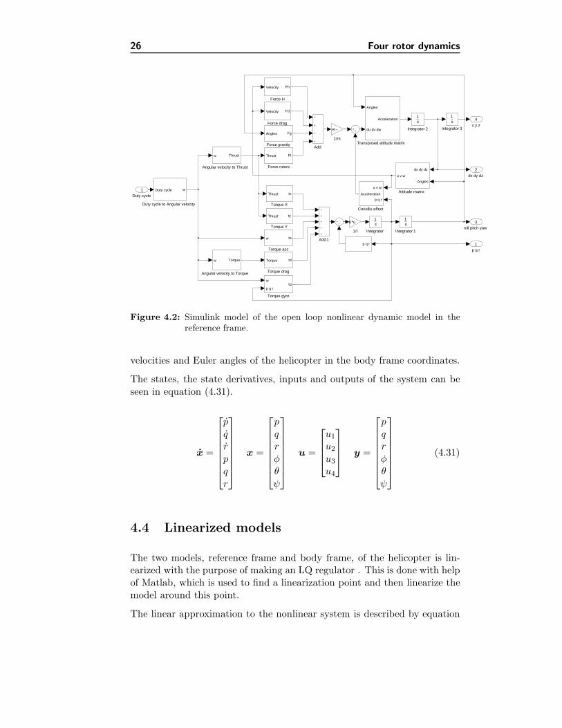
Figure 4.2: Simulink model of the open loop nonlinear dynamic model in thereference frame.
velocities and Euler angles of the helicopter in the body frame coordinates.
The states, the state derivatives, inputs and outputs of the system can beseen in equation (4.31).
x =
⎡⎢⎢⎢⎢⎢⎢⎣
pqrpqr
⎤⎥⎥⎥⎥⎥⎥⎦
x =
⎡⎢⎢⎢⎢⎢⎢⎣
pqrφθψ
⎤⎥⎥⎥⎥⎥⎥⎦
u =
⎡⎢⎢⎣u1
u2
u3
u4
⎤⎥⎥⎦ y =
⎡⎢⎢⎢⎢⎢⎢⎣
pqrφθψ
⎤⎥⎥⎥⎥⎥⎥⎦
(4.31)
4.4 Linearized models
The two models, reference frame and body frame, of the helicopter is lin-earized with the purpose of making an LQ regulator . This is done with helpof Matlab, which is used to find a linearization point and then linearize themodel around this point.
The linear approximation to the nonlinear system is described by equation

4.4 Linearized models 27
roll pitch yaw
2
p q r
1
Torque gyro
w
p q rtg
Torque drag
Torque td
Torque acc
w ta
Torque Y
Thrust ty
Torque X
Thrust tx
Integrator 1
1s
Integrator
1s
Duty cycle to Angular velocity
Duty cycle w
Angular velocity to Torque
w Torque
Angular velocity to Thrust
w Thrust
Add1
1/I
K*u
p q r
In1
1
Figure 4.3: Simulink model of the open loop nonlinear dynamic model in bodyframe. The Angular velocity to thrust and Angular velocity to torqueblocs are discussed in appendix I
(4.32), (18, p. 40).∆x(t) = A∆x(t) + B∆u(t) (4.32)
Where the ∆’s denote the deviation from the linearization point. MatricesA and B are:
A =∂f(x0,u0)
∂x, B =
∂f(x0,u0)∂u
(4.33)
In equation (4.33), x0 and u0 are the stationary values, in this case thevalues corresponding to hover.
The initial guess of a linearization point is done on the basis of measurementsfor thrust and duty cycle which are shown in appendix I. The duty cycle isthe control signal for the rotors of the helicopter and the thrust is the lift ofeach rotor. Hover state is when the trust from the rotors is just enough toovercome the gravitational force and the helicopter is still in the air.
By using the trim function in Matlab the linearization point is generatedapplying the initial guess for the input signal.
4.4.1 Linearized model in reference frame
The linearized model in reference frame is found in this section. The trimfunction generates the following initial input signal values:
u0(1) = 0.4013u0(2) = 0.3864u0(3) = 0.3871u0(4) = 0.3705
(4.34)

28 Four rotor dynamics
The input signals are are presented in duty cycle from 0 (0%) to 1 (100%).
Now that the input signals for hover are found, the linearizion of the he-licopter model can take place. The linearization is done with the Matlabfunction linmod, which takes the initial/stationary values for the states andcontrol signals. The stationary values for the states are equal to zero. Thelinear state space model is on the form:
x(t) = Ax(t) + Bu(t), y(t) = Cx(t) + Du(t) (4.35)
Where the state space matrices A and B are as follows:
A =
⎡⎢⎢⎢⎢⎢⎢⎢⎢⎢⎢⎢⎢⎢⎢⎢⎢⎢⎢⎢⎣
0 −6.3613 0 0 0 0 0 0 0 0 0 06.4007 0 0 0 0 0 0 0 0 0 0 0
0 0 1 0 0 0 0 0 0 0 0 00 0 0 1 0 0 0 −9.82 0 0 0 00 0 0 0 1 0 9.82 0 0 0 0 00 0 0 0 0 1 0 0 0 0 0 00 0 0 0 0 0 1 0 0 0 0 00 0 0 0 0 0 0 1 0 0 0 00 0 0 0 0 0 0 0 1 0 0 00 0 0 0 0 0 0 0 0 1 0 00 0 0 0 0 0 0 0 0 0 1 00 0 0 0 0 0 0 0 0 0 0 1
⎤⎥⎥⎥⎥⎥⎥⎥⎥⎥⎥⎥⎥⎥⎥⎥⎥⎥⎥⎥⎦
B =
⎡⎢⎢⎢⎢⎢⎢⎢⎢⎢⎢⎢⎢⎢⎢⎢⎢⎢⎢⎢⎣
181.7491 −183.0452 −181.5290 176.7712182.8752 −184.1794 182.6537 −177.8664−58.5946 −58.9435 57.3055 53.9644
0 0 0 00 0 0 0
−12.1935 −12.2805 −12.1787 −11.85950 0 0 00 0 0 00 0 0 00 0 0 00 0 0 00 0 0 0
⎤⎥⎥⎥⎥⎥⎥⎥⎥⎥⎥⎥⎥⎥⎥⎥⎥⎥⎥⎥⎦
The C matrix is the output matrix. The outputs are, angles [φ, θ, ψ] andthe position [x, y, z]. These output are used to generate a reference matrixused for simulations. The C matrix is:

4.4 Linearized models 29
C =
⎡⎢⎢⎢⎢⎢⎢⎣
0 0 0 0 0 0 1 0 0 0 0 00 0 0 0 0 0 0 1 0 0 0 00 0 0 0 0 0 0 0 1 0 0 00 0 0 0 0 0 0 0 0 1 0 00 0 0 0 0 0 0 0 0 0 1 00 0 0 0 0 0 0 0 0 0 0 1
⎤⎥⎥⎥⎥⎥⎥⎦
And the D matrix:
D =
⎡⎢⎢⎢⎢⎢⎢⎣
0 0 0 00 0 0 00 0 0 00 0 0 00 0 0 00 0 0 0
⎤⎥⎥⎥⎥⎥⎥⎦
The helicopter model in reference frame has a complex conjugate pole pair in0±6.381i and ten poles in 0. Since all the poles are placed on the imaginaryaxis the helicopter is marginally stable.
To verify that the model is controllable, the controllability matrix is foundby using following equation:
M c = [B AB A2B ... An−1B] (4.36)
The controllability matrix has full rank and the system is therefore control-lable.
4.4.2 Linearized model in body frame
The procedure of finding the linearized model in body frame is the same asfor the model in reference frame. The trimmed values are:
u0(1) = 0.3956u0(2) = 0.3807u0(3) = 0.3812u0(4) = 0.3644
(4.37)
The trimmed values for the reference frame model, see equation (4.34) arenot the same as the trimmed values for the body frame model, see equation(4.37). This happens because the trim function only considers the attitudeand not the altitude of the helicopter when used with the body frame model.This means that the helicopter is not necessarily stable with respect to

30 Four rotor dynamics
altitude using the trimmed values seen in equation (4.37). The state spacematrices A and B are as follows:
A =
⎡⎢⎢⎢⎢⎢⎢⎣
0 −6.2723 0 0 0 06.3111 0 0 0 0 0
0 0 0 0 0 01 0 0 0 0 00 1 0 0 0 00 0 1 0 0 0
⎤⎥⎥⎥⎥⎥⎥⎦
B =
⎡⎢⎢⎢⎢⎢⎢⎣
180.8002 −182.0131 −181.0361 176.1681181.9204 −183.1409 182.1577 −177.2596−58.4693 −58.6113 57.2476 53.9213
0 0 0 00 0 0 00 0 0 0
⎤⎥⎥⎥⎥⎥⎥⎦
The output matrix C includes all the states, angular velocities [p q r]′ andangles [φ θ ψ]′.
C =
⎡⎢⎢⎢⎢⎢⎢⎣
1 0 0 0 0 00 1 0 0 0 00 0 1 0 0 00 0 0 1 0 00 0 0 0 1 00 0 0 0 0 1
⎤⎥⎥⎥⎥⎥⎥⎦
D =
⎡⎢⎢⎢⎢⎢⎢⎣
0 0 0 00 0 0 00 0 0 00 0 0 00 0 0 00 0 0 0
⎤⎥⎥⎥⎥⎥⎥⎦
The helicopter model in body frame has a complex conjugated pole pair in0 ± 6.29i and ten poles in 0. As for the helicopter model in the referenceframe the system is marginally stable. The controllability matrix, equation4.36, has full rank and therefore the model is controllable.
4.5 Open loop simulations of model in body frame
In this section the nonlinear and linear models in body frame are simulatedand compared. If figure 4.4 the six states are shown, angular velocities[p q r]′ and angles [φ θ ψ]′.
The two models are given initial values for the angular velocity around they-axis, q. The imaginary pole pairs’ natural frequencies 6.29[rads ] can be

4.6 Motor model 31
seen on the plots of the angular velocities p and q for both models. Theseoscillations are naturally transferred to the angles. The angular velocitiesp and q for both models seem to be identical, while the angular velocity rfor the linear model drifts away from the nonlinear model with 0.0017[ rads ].Angles roll, φ, and yaw, ψ for the linear model also drift away from thenonlinear model.
These deviations between the linear and the nonlinear model are due to theinitial values for the states and input signals, the slightest deviation cancause the linear model to drift away from the nonlinear model.
4.6 Motor model
The motors of the helicopter are brushless DC motors which drive the pro-pellers of the heilcopter. Brushless DC motors dynamics can by linearlymodeled with the same principles as a brushed DC motor, though the con-trol is different, see chapter 6.4 for description of brushless motors and thecontrol. In figure 4.5 a block diagram of a DC motor is shown, see (26, Ch.2).
The input signal to the model is the armature voltage Va[V ], which is thevoltage over the armature windings. The the back electromotive force (backemf) voltage, Ve[V ], counteracts the armature voltage and is therefore sub-tracted from the armature voltage Va[V ]. The back emf voltage is inducedin the armature of the rotor proportionally to the angular velocity of themotor determined by Ke[ V srad ] where Ke is the back emf constant.
The electrical part of the motor is described by the block 1Ra+sLa
, whereRa[Ω] is the impedance and La[H] the inductance of the armature windings.The momentMu[Nm] produced by the armature is proportional to armaturecurrent Ia[A] multiplied by the moment constant of the motor Kt[NmA ].
This moment is affected by the friction of the motor Mf [Nm], which isproportional to the angular velocity of the motor, and the external loadMb[Nm] (in this case the propellers of the helicopter). Jm[kgm2] is themoment of inertia of the motor giving the acceleration of the motor andby integrating the acceleration of the motor the angular velocity ωm[ rads ] isfound.
There are numerous constants that have to be measured for the model ofthe motor. The measurements can lead to great uncertainties for the model.Therefore a different approach was taken in modeling the motor with thepropellers, the combination of the motor and propeller is called a rotor.
In order to make the model measurements of the rotor, angular velocity

32 Four rotor dynamics
0 2 4 6 8 10 12 14 16 18 20−0.2
0
0.2p
Ang
ular
vel
ocity
[rad
/s]
NonlinearLinear
0 2 4 6 8 10 12 14 16 18 20−0.2
0
0.2q
Ang
ular
vel
ocity
[rad
/s]
NonlinearLinear
0 2 4 6 8 10 12 14 16 18 20−0.02
0
0.02
0.04r
Ang
ular
vel
ocity
[rad
/s]
NonlinearLinear
0 2 4 6 8 10 12 14 16 18 20−0.1
0
0.1Roll
Ang
les
[rad
]
NonlinearLinear
0 2 4 6 8 10 12 14 16 18 20−0.02
0
0.02Pitch
Ang
les
[rad
]
NonlinearLinear
0 2 4 6 8 10 12 14 16 18 20−0.2
0
0.2
0.4Yaw
Ang
les
[rad
]
Time [s]
NonlinearLinear
Figure 4.4: Open loop response for the body frame model, with initial angularvelocity q = 0.1[ rad
s ].

4.6 Motor model 33
Figure 4.5: Motor model.
measurements were done around hover. By giving the rotors a step on theinput signal (duty cycle) while measuring the angular acceleration time, therotors time constant can be derived. The time constant is the time it takesthe output (angular velocity of rotor) to reach 63.2% its final value, fromthe step start. Assuming that inductance of the motor is very small therotor can be modeled as a first order system with time constant τr. Thetime constant was measured τr = 0.05[s] and is considered to be the samefor all rotors. The transfer function is:
ωrDr
=1
τrs+ 1
Where Dr is the duty cycle, ωr the angular velocity of the rotor and τr thetime constant for the rotor.
The input to the rotor is the duty cycle and its output is the angular ve-locity. Therefore a function describing the relations between duty cycle andangular velocity is made from measurements, see appendix I. In figure 4.6the Matlab/Simulink model of the rotor is shown.
w
1
Integrator
1s
Gain 1
−K−
Gain
−K−
Duty cycle to Angular velocity
f(u)
Duty cycle
1
Figure 4.6: Simulink model of helicopter rotor. The gains are equal to 1τr
.

34 Four rotor dynamics
Chapter 5
Controller design
In this chapter a controller for the four rotor helicopter is designed. Be-cause the mathematical model of the helicopter presented in chapter 4 ismarginally stable, a controller is designed with the goal to make the heli-copter stable.
The controller specifications for a pilot augmented system have been sug-gested in (31). There the rise time is tr < 1[s], settling time ts < 5[s] anddamping ratio 0.4 ≤ ζ ≤ 1.3. The controller will be designed using thesespecifications.
The model of the helicopter is a MIMO system (Multiple Input MultipleOutput system) and therefore a traditional controller, such as PID con-troller (Proportional Integral Derivative), would require quite a lot of timefor hand tuning. Therefore a Linear Quadratic Regulator (LQR), whichis a MIMO linear closed loop controller, is chosen . The LQ regulator isdescribed in next section, using theory from (18, ch.5).
5.1 Linear Quadratic Regulator
The helicopter model described in chapter 4 is an nonlinear model, thereforethe model needs to be linearized to apply the LQ regulator. The linearizationpoint is when the helicopter is in a hovering state, see chapter 4.
The LQ regulator is an optimal controller with the goal of minimizing or

36 Controller design
maximizing the performance index to achieve a qualified controller. Theperformance index is a measure of the quality of the controller.
Figure 5.1: A sample of a regulator time response where the object for the regu-lator is to make the output signal y(t) reach the stationary point r0,(18, Figure 5.2).
In figure 5.1 a typical regulator problem is shown. The object for the regula-tor is to make the output signal y(t) reach the stationary point r0, as fast aspossible without too much overshoot. The grey area on the plot illustratesthe error in the system where the best controller is the one that minimizesthis area. Equation 5.1 is the performance index of the illustrated figure 5.1.The performance index is equal to 0 when there is no error in the system,this is achieved when the output signal y(t) is equal to the stationary pointr0 for t = 0 → ∞. The control signal does not have limitations in equation5.1 which is not the case in the four rotor helicopter construction.
∫ ∞
0| y(t) − r0 | dt (5.1)
The control signal has physical restrictions and therefore the cost functionhas to take the limitations of control signal into account. Since the systemis linearized around an operating point, hover in the helicopter case, thedeviations from that point should be added to the cost function.
Equation 5.2 is the performance index for the LQ regulator. R1 is theweight matrix for the states and R2 is the weight matrix for the controlsignals, where ∆x(t) = x(t)− x0 and ∆u(t) = u(t)− u0 are the incremental

5.1 Linear Quadratic Regulator 37
states and control signals.
J =∫ t1
t0
[∆xT (t)R1∆x(t) + ∆uT (t)R2∆u(t)]dt (5.2)
These weight matrices will determine how much deviation of x(t) and u(t),respectively, from the stationary points will be added to the cost function.The combination of these two parts of the cost function will set the speedof the control system.
The objective is to make a steady state LQ regulator where the helicoptermodel is linearized around the hover state. The linearized model is on thestate space form:
x(t) = Ax(t) + Bu(t) (5.3)
Equations 5.4 and 5.5 are used to select the weights of the weight matricesfor the states, R1, and the control signals, R2, respectively.
[R1]ii =1
max([xi(t)]2)(5.4)
[R2]jj =1
max([uj(t)]2)(5.5)
To determine the optimal control matrix, K, for the time invariant systemthe Algebraic Riccati Equation (ARE) has to be solved:
0 = ATP + PA + R1 − P BR−12 BTP (5.6)
By solving the Riccati equation, the feedback gain K can be obtained byusing equation 5.7.
K = R−12 BTP (5.7)
Thereby the optimal gain matrix K can be used to close the loop from thestates of the system, x(t), to the control signals, u(t).
In figure 5.2 the state space model is illustrated with the LQ regulator.

38 Controller design
Figure 5.2: LQ regulator in a closed loop system with full state feedback, (18,Figure 4.4).
5.2 Designing a continuous LQR for attitude andposition stabilization
In this section the method described in section 5.1 is used to design a contin-uous LQ regulator for the helicopter. The controller designed is a full statefeedback controller. This is done for simulation purpose, making it possibleto fly the helicopter model to desired position in the reference frame.
The object is to design a controller that makes it possible for a humanpilot to fly the helicopter. The closed loop response time must therefore beadjusted to fit within the range of human pilot perception.
The first step is to choose the restrictions for the weights of the weightmatrices for the states R1 and the control signals R2 by using equations 5.4and 5.5 respectively. The maximum-values for R1 are:
[p, q, r] = 2.62[rad/s][x, y, z] = 1.9[m/s][φ, θ, ψ] = 0.262[rad][x, y, z] = 0.2[m]
The maximum-values for R2 are:
[u1, u2, u3, u4] = 0.1
The state weight matrix R1 is diagonal with elements inversely proportionalto the square of the max-values of the state variable, and is as follows:
R1 =

5.2 Designing a continuous LQR for attitude and position stabilization39
⎡⎢⎢⎢⎢⎢⎢⎢⎢⎢⎢⎢⎢⎢⎢⎢⎢⎢⎢⎢⎣
12.622 0 0 0 0 0 0 0 0 0 0 00 1
2.622 0 0 0 0 0 0 0 0 0 00 0 1
2.622 0 0 0 0 0 0 0 0 00 0 0 1
1.92 0 0 0 0 0 0 0 00 0 0 0 1
1.92 0 0 0 0 0 0 00 0 0 0 0 1
1.92 0 0 0 0 0 00 0 0 0 0 0 1
0.2622 0 0 0 0 00 0 0 0 0 0 0 1
0.2622 0 0 0 00 0 0 0 0 0 0 0 1
0.2622 0 0 00 0 0 0 0 0 0 0 0 1
0.22 0 00 0 0 0 0 0 0 0 0 0 1
0.22 00 0 0 0 0 0 0 0 0 0 0 1
0.22
⎤⎥⎥⎥⎥⎥⎥⎥⎥⎥⎥⎥⎥⎥⎥⎥⎥⎥⎥⎥⎦
The input weight matrix is:
R2 =
⎡⎢⎢⎣
10.12 0 0 00 1
0.12 0 00 0 1
0.12 00 0 0 1
0.12
⎤⎥⎥⎦
The max-values for the states are chosen considering the helicopter to beflown indoors. The angular velocity values are the dynamic range valuesgiven for the gyroscope sensor used to measure the angular velocity for thephysical four rotor helicopter, see data sheet for gyroscopes (10). The finalvalues for the restriction presented above were found by simulating the stepresponse in figure 5.4 and adjusting the values until a desired response wasachieved.
The optimal gain matrix K is then found by using the lqr function inMatlab, and is:
K =[0.0361 0.0365 −0.0459 −0.1714 0.0930 −0.1026 0.2474 0.4471 −0.1959 −0.3093 0.1681 −0.2456
−0.0365 −0.0362 −0.0453 0.1720 −0.0951 −0.1020 −0.2533 −0.4479 −0.1935 0.3109 −0.1715 −0.2445−0.0367 0.0367 0.0441 −0.0954 −0.1732 −0.1060 −0.4512 0.2540 0.1860 −0.1721 −0.3128 −0.2515
0.0364 −0.0365 0.0451 0.0929 0.1707 −0.1089 0.4463 −0.2475 0.1884 0.1675 0.3074 −0.2581
]
To be able to simulate the closed loop system of the helicopter with a ref-erence input in the reference frame, a reference transformation gain matrixis implemented. The inputs to the matrix are the position and angles ofthe helicopter, and the outputs are the control signals, see figure 5.3 of theMatlab/Simulink model.
The reference transformation gain matrix is found by using equations (5.8)and (5.9), from (21, p. 5.40).
M = C(A − BK)−1B (5.8)

40 Controller design
StepZ
StepY
StepX
Step Yaw
Step Roll
Step Pitch
Saturation of control signal
Referancegain matrix F
K*u
LQR gain matrix K
K*u
Control signal for hover
u04rotor helicopter
Ud
p q r
dotx doty dotz
roll pitch yaw
x y z
Figure 5.3: Matlab/Simulink model of the four rotor helicopter model and thecontinuous LQ regulator.
F = −(MTM)−1MT (5.9)
To find out whether the closed loop system is stable, the poles for the systemare found. The eigenvalues for the poles in the system are complex conju-gated which means that the poles are in a second order system. A secondorder system can be described with the transfer function:
Y (s)U(s)
=ω2n
s2 + 2ζωns+ ω2n
(5.10)
Where ωn is the natural frequency and ζ the damping factor. The secondorder system shows the connection between the states of the system, howeach angle is dependent on corresponding angular velocity and how eachposition is dependent on corresponding velocity.
In finding eigenvalues, damping factors, natural frequencies and time con-stants, the closed loop matrix Ac is found. That is done using the followingequation:
x(t) = Acx(t) = (A − BK)x(t)⇒ Ac = A − BK
The eigenvalues, damping, natural frequencies and time constants of theclosed loop system, Ac are shown in table 5.1. All the poles lie in the lefthalf-plane of the s-plane, and therefore the closed loop system is stable.
Equations 5.11, 5.12 and 5.13 can be used to find the natural frequencies,damping ratios and time constants for the system poles.
ωn =√α2 + β2 (5.11)
5.2 Designing a continuous LQR for attitude and position stabilization41
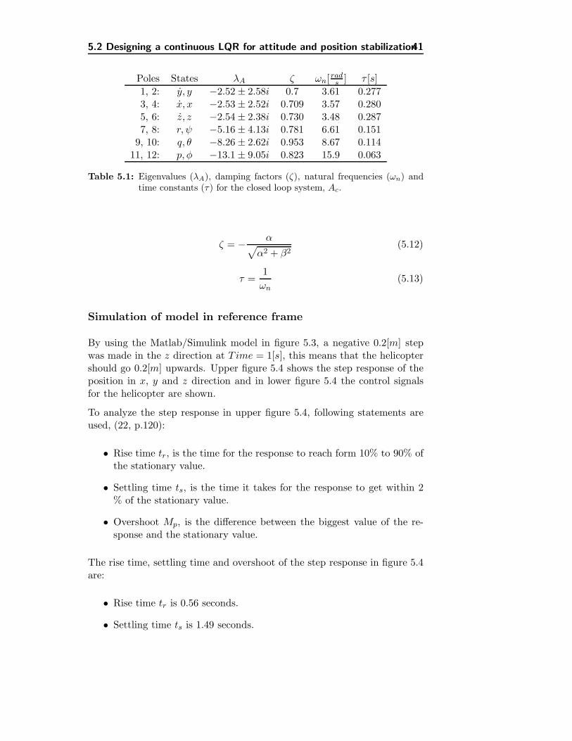
Poles States λA ζ ωn[ rads ] τ [s]1, 2: y, y −2.52 ± 2.58i 0.7 3.61 0.2773, 4: x, x −2.53 ± 2.52i 0.709 3.57 0.2805, 6: z, z −2.54 ± 2.38i 0.730 3.48 0.2877, 8: r, ψ −5.16 ± 4.13i 0.781 6.61 0.151
9, 10: q, θ −8.26 ± 2.62i 0.953 8.67 0.11411, 12: p, φ −13.1 ± 9.05i 0.823 15.9 0.063
Table 5.1: Eigenvalues (λA), damping factors (ζ), natural frequencies (ωn) andtime constants (τ) for the closed loop system, Ac.
ζ = − α√α2 + β2
(5.12)
τ =1ωn
(5.13)
Simulation of model in reference frame
By using the Matlab/Simulink model in figure 5.3, a negative 0.2[m] stepwas made in the z direction at T ime = 1[s], this means that the helicoptershould go 0.2[m] upwards. Upper figure 5.4 shows the step response of theposition in x, y and z direction and in lower figure 5.4 the control signalsfor the helicopter are shown.
To analyze the step response in upper figure 5.4, following statements areused, (22, p.120):
• Rise time tr, is the time for the response to reach form 10% to 90% ofthe stationary value.
• Settling time ts, is the time it takes for the response to get within 2% of the stationary value.
• Overshoot Mp, is the difference between the biggest value of the re-sponse and the stationary value.
The rise time, settling time and overshoot of the step response in figure 5.4are:
• Rise time tr is 0.56 seconds.
• Settling time ts is 1.49 seconds.

42 Controller design
0 0.5 1 1.5 2 2.5 3 3.5 4 4.5 5−0.25
−0.2
−0.15
−0.1
−0.05
0
0.05
0.1Position
Pos
ition
[m]
xyz
0 0.5 1 1.5 2 2.5 3 3.5 4 4.5 50.34
0.36
0.38
0.4
0.42
0.44
0.46Control signals
Dut
y cy
cle
Time [s]
U1U2U3U4
Figure 5.4: Step response of the helicopter model with LQR. The position isshown on the upper plot and the control signals below.
• Overshoot Mp is 3.5%.
The settling time and rise time are reasonable and the overshoot of 0.007[m]is considered to be trivial. The control signals are shown in figure 5.4, pre-sented as the duty cycle. The control signals do not saturate so the LQregulator is working within the limits of the control signal. These responsesgive an show that the model of the helicopter behaves correctly at the lin-earization point.
The LQ regulator was also tested by setting the initial value for the velocityin the x-direction (x) equal to 0.5[m/s]. The reference signals are zerothroughout the simulation. The results of the simulations are illustrated infigure 5.5.
The controller starts to react immediately and gives rotors 1 and 3 a boost, tocorrect this pitch and change of position. This forces the helicopter to pitchbackwards, increasing the pitch angle to 0.24[rad]. This initial velocity alsohas influence on the position of the helicopter, causing it to move 0.11[m]in the x-direction and losing height to 0.02[m]. These changes in control

5.2 Designing a continuous LQR for attitude and position stabilization43
signal shifts the velocity in the x-direction backwards causing the helicopterto move towards zero. The controller brings the helicopter to the trimmedcontrol values, in 2.5 seconds. As in the test before the controller and themodel response correctly, this time to the initial value of the velocity in thex-direction.
The swings in the angular velocity, p, around the x-axis from 0 seconds to1 second are due to the time constants of the rotor interacting with timeconstants of the helicopter rotors causing these swings. The lower the timeconstants are the smaller the swings become. The rotors time constants alsoinfluence the angular velocity, q, around the y-axis which leads to the angles’roll (φ) and pitch (θ).
The oscillations on the angular velocity p and roll angle φ are slightly fasterthan their corresponding natural frequencies. The frequency on the plot forthe angular velocity is 22rads (3.5Hz) while the natural frequency in table5.1 is 15.9rads (2.5Hz). This difference is due to the time constants of therotors. If the time constants of the rotors are made smaller the frequencyof the oscillations gets closer 15.9 rads . This is also the case for the angularvelocity q and pitch angle θ. The natural frequency for the velocity x is3.57[ rads ] (0.57Hz) which can be seen on the response for the velocity x.

44 Controller design
0 0.5 1 1.5 2 2.5 3 3.5 4 4.5 5
0.35
0.4
0.45
0.5Control signals
Dut
y cy
cle
U1U2
0 0.5 1 1.5 2 2.5 3 3.5 4 4.5 5
0.35
0.4
0.45
0.5
Dut
y cy
cle
U3U4
0 0.5 1 1.5 2 2.5 3 3.5 4 4.5 5−2
0
2States
Ang
ular
vel
ocity
[rad
/s]
pqr
0 0.5 1 1.5 2 2.5 3 3.5 4 4.5 5−0.5
0
0.5
Vel
ocity
[m/s
]
dxdydz
0 0.5 1 1.5 2 2.5 3 3.5 4 4.5 5−0.5
0
0.5
Ang
les
[rad
]
rollpitchyaw
0 0.5 1 1.5 2 2.5 3 3.5 4 4.5 5−0.2
0
0.2
Time [s]
Pos
ition
[m]
xyz
Figure 5.5: Results of simulation of the continuous LQR with an initial state valueof 1[m/s] for velocity x. The control signals are plotted on the firsttwo figures and the states are on the next four figures. The simulationtime is 5 seconds.

5.3 Designing a reduced continuous LQR for attitude stabilization 45
5.3 Designing a reduced continuous LQR for atti-tude stabilization
The physical helicopter has gyroscopic sensors which measure the angular ve-locities [p, q, r] and, by integrating the angular velocities, the angles [φ, θ, ψ]of the helicopter. This means that a full state feedback controller is not anoption. Therefore an LQ regulator is designed for the four rotor helicopterin body frame, using the method presented in section 5.1.
As in section 5.3 the object is to design a controller that has a closed loopresponse time that fits within the range of human pilot perception.
The weights for the state weight matrix R1 and the input weight matrix arethe same as for the controller designed in section 5.2 without the acceleration[x, y, z] and position [x, y, z]. The state weight matrix max-values are:
[p, q, r] = 2.62[rad/s][φ, θ, ψ] = 0.262[rad]
The maximum-values for R2 are:
[u1, u2, u3, u4] = 0.1
The control matrix for the model in body frame is:
K2 =
⎡⎢⎢⎣
0.0291 0.0297 −0.0466 0.1270 0.2368 −0.1972−0.0297 −0.0293 −0.0460 −0.1312 −0.2376 −0.1946−0.0298 0.0297 0.0437 −0.2388 0.1305 0.18570.0293 −0.0295 0.0442 0.2356 −0.1277 0.1862
⎤⎥⎥⎦
The closed loop eigenvalues, damping factors, natural frequencies and timeconstants for the body frame model are shown in table 5.2.
Poles States λA ζ ωn[ rads ] τ [s]1, 2: r, ψ −5.15 ± 4.13i 0.780 6.60 0.1523, 4: q, θ −8.27 ± 2.71i 0.950 8.70 0.1155, 6: p, φ −13.1 ± 9.0i 0.824 15.9 0.063
Table 5.2: Eigenvalues (λA), damping factors (ζ), natural frequencies (ωn) andtime constants (τ) for the closed loop body frame system, Ac.
To see how the closed loop system behaves, it is simulated with initial con-ditions on the angular velocity q of π/2[ rads ] around the y-axis. Figure 5.6shows the results of the simulation.

46 Controller design
The initial angular velocity causes the helicopter to pitch backwards to0.09[rad] and roll to the left to −0.03[ rads ]. The controller reacts to theinitial state value and gives rotors 1 and 3 higher control signal to bring thehelicopter to steady state, which takes about 1[s].
As in the simulation for the full state feedback controller, the swings in an-gular velocity, p, around the x-axis, are due to the rotors’ time constants in-tervening with time constants of the helicopter. The swings become smalleras the time constants of the rotor are lower.

5.3 Designing a reduced continuous LQR for attitude stabilization 47
0 0.5 1 1.5 2 2.5 3
0.35
0.4
0.45Control signals
Dut
y cy
cle
U1U2
0 0.5 1 1.5 2 2.5 3
0.35
0.4
0.45
Dut
y cy
cle
U3U4
0 0.5 1 1.5 2 2.5 3−1
0
1
2States
Ang
ular
vel
ocity
[rad
/s]
pqr
0 0.5 1 1.5 2 2.5 3−0.05
0
0.05
0.1
0.15
Ang
les
[rad
]
Time [s]
rollpitchyaw
Figure 5.6: Results of simulation of the model in body frame using LQR with aninitial state value of π/2 for angular velocity q. The control signalsare plotted on the first two figures and the states on the next two.

48 Controller design
5.4 Discrete Linear Quadratic Regulator
The physical four rotor helicopter has a microprocessor where the controlsystem is implemented, see chapter 6. This means that the controlling ofthe helicopter takes place on a digital platform. In this section it is shownhow the LQ regulator is discretized.
The linearized state space model of the helicopter needs to be discretized,as shown in equation 5.14.
x(k + 1) = Fx(k) + Gu(k) (5.14)
To determine the optimal control matrix, K, the Riccati differential equation5.15 has to be solved.
P d = R1d + F T [P d − P dG(R2d + GTP dG)−1GTP d]F (5.15)
Where the weight matrices are transformed from continuous time to discretetime by using equations:
R1d = R1 · Ts (5.16)R2d = R2 · Ts
By solving the discrete Riccati equation the feedback gain K can be obtainedby using the following equation:
Kd = [R2d + GTP dG]−1GTP dF (5.17)
5.5 Designing a discrete LQR
The method described in section 5.4 is used in this section to design a dis-crete LQ regulator. A linearized state space model is found with sample timeof 0.01[s] and a discrete LQ regulator found from that model. The contin-uous LQ regulator from section 5.3 is then compared with two discrete LQregulators, one with 0.01[s] sample time and the other with 0.02[s] sampletime. This is done to see if the performance of the regulator is reduced whenchanging from continuous LQ regulator to a discrete LQ regulator and tosee if a different sample time has much effect on the discrete LQ regulatorsperformance.
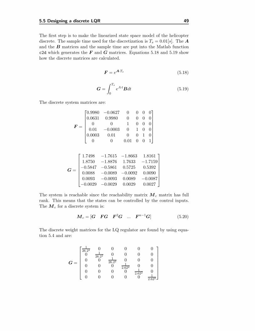
5.5 Designing a discrete LQR 49
The first step is to make the linearized state space model of the helicopterdiscrete. The sample time used for the discretization is Ts = 0.01[s]. The Aand the B matrices and the sample time are put into the Matlab functionc2d which generates the F and G matrices. Equations 5.18 and 5.19 showhow the discrete matrices are calculated.
F = eA·Ts (5.18)
G =∫ Ts
0eA·tBdt (5.19)
The discrete system matrices are:
F =
⎡⎢⎢⎢⎢⎢⎢⎣
0.9980 −0.0627 0 0 0 00.0631 0.9980 0 0 0 0
0 0 1 0 0 00.01 −0.0003 0 1 0 0
0.0003 0.01 0 0 1 00 0 0.01 0 0 1
⎤⎥⎥⎥⎥⎥⎥⎦
G =
⎡⎢⎢⎢⎢⎢⎢⎣
1.7498 −1.7615 −1.8663 1.81611.8750 −1.8876 1.7633 −1.7159−0.5847 −0.5861 0.5725 0.53920.0088 −0.0089 −0.0092 0.00900.0093 −0.0093 0.0089 −0.0087−0.0029 −0.0029 0.0029 0.0027
⎤⎥⎥⎥⎥⎥⎥⎦
The system is reachable since the reachability matrix M c matrix has fullrank. This means that the states can be controlled by the control inputs.The M c for a discrete system is:
M c = [G FG F 2G ... F n−1G] (5.20)
The discrete weight matrices for the LQ regulator are found by using equa-tion 5.4 and are:
G =
⎡⎢⎢⎢⎢⎢⎢⎣
126.22 0 0 0 0 00 1
26.22 0 0 0 00 0 1
26.22 0 0 00 0 0 1
2.622 0 00 0 0 0 1
2.622 00 0 0 0 0 1
2.622
⎤⎥⎥⎥⎥⎥⎥⎦

50 Controller design
R2d =
⎡⎢⎢⎣
112 0 0 00 1
12 0 00 0 1
12 00 0 0 1
12
⎤⎥⎥⎦
The discrete LQ regulator gain matrix is now found by using dlqr functionin Matlab. The gain matrix is:
Kd =
⎡⎢⎢⎣
0.0276 0.0270 −0.0452 0.1138 0.2128 −0.1872−0.0282 −0.0265 −0.0446 −0.1179 −0.2135 −0.1849−0.0270 0.0282 0.0423 −0.2149 0.1171 0.17620.0266 −0.0280 0.0429 0.2122 −0.1146 0.1770
⎤⎥⎥⎦
To find the eigenvalues for the discrete closed loop system the closed loopsystem matrix needs to be found. The closed loop matrix is found by usingequation 5.21.
F c = F − GK (5.21)
The discrete eigenvalues, λF , are shown in table 5.3. The damping factors,natural frequencies and time constants are the same as for the continuousclosed loop system shown in table 5.2.
Poles λF λA ζ ωn[ rads ] τ [s]1: 0.949 + 0.0392i −5.15 + 4.13i 0.780 6.60 0.1522: 0.949 − 0.0392i −5.15 − 4.13i 0.780 6.60 0.1523: 0.920 + 0.0249i −8.27 + 2.71i 0.950 8.70 0.1154: 0.920 − 0.0249i −8.27 − 2.71i 0.950 8.70 0.1155: 0.874 + 0.0789i −13.1 + 9.0i 0.824 15.9 0.0636: 0.874 + 0.0789i −13.1 − 9.0i 0.824 15.9 0.063
Table 5.3: The discrete eigenvalues corresponding to the continuous eigenvalues,damping factors, natural frequencies and time constants shown in table5.2.
The relations between the continuous eigenvalues, λA, and the discreteeigenvalues,λA, are shown in the following equation:
λF = eλATs (5.22)
All the discrete poles lie inside the unit circle and are therefore stable. Thisis to be expected since the continuous poles are stable.

5.5 Designing a discrete LQR 51
Two discrete LQ regulators, with 0.01[s] and 0.02[s] sample time, are com-pared with the continuous LQ regulator designed in section 5.3. They aresimulated with the initial values for the angular velocity around the y-axis,q. Figure 5.7 shows the results of the simulation. The angular velocities, pand q are plotted on the top two plots and the angles roll (φ) and pitch (θ)the bottom two.
The response for the discrete controller and the continuous controller aresimilar. This was expected since the discrete controller is based on thecontinuous controller. The simulations show that the smaller the samplingtime is the more the discrete response looks like the continuous response,which is as to be expected.
Even though the discrete LQ regulators are similar to the continuous one,they do not settle the states to steady state as quickly and have more over-shoot. The discrete LQ regulator with sample time of 0.02[s] takes moretime to settle the states to steady state than the regulator with 0.01[s] andhas more overshoot. The difference between the two discrete regulators issmall, showing that both regulators should be able to control the four rotorhelicopter. Sample times bigger than 0.02[s] have been tested (not reported).These give a longer settling time and higher overshoot, and are therefore notconsidered good candidates for controlling the four rotor helicopter.

52 Controller design
0 0.5 1 1.5 2 2.5 3−0.5
0
0.5
1p
Ang
ular
vel
ocity
[rad
/s]
ContinuousDiscrete Ts=0.01Discrete Ts=0.02
0 0.5 1 1.5 2 2.5 3−1
0
1
2q
Ang
ular
vel
ocity
[rad
/s]
ContinuousDiscrete Ts=0.01Discrete Ts=0.02
0 0.5 1 1.5 2 2.5 3−0.04
−0.02
0
0.02
0.04Roll
Ang
les
[rad
]
ContinuousDiscrete Ts=0.01Discrete Ts=0.02
0 0.5 1 1.5 2 2.5 3−0.05
0
0.05
0.1
0.15Pitch
Ang
les
[rad
]
Time [s]
ContinuousDiscrete Ts=0.01Discrete Ts=0.02
Figure 5.7: Comparing continuous LQR with discrete LQR with 0.01 and 0.02second sampling time.

Chapter 6
Hardware
The topic of this chapter is the electrical hardware used in the project.Figure 6.1 illustrates a block diagram of the hardware structure.
The flight controller board is connected to a 3 cell Lithium-ion polymerbattery (LIPO battery), which powers all of the devices including the motors.The microprocessor is the main control unit. It has an input that reads froma receiver, an input for measurements from gyroscopes, a serial connectionto a Bluetooth device and a two wire serial connection to motor controllers.In the following section, the hardware is described in more detail.
6.1 The flight controller
The flight controller board is developed by the SACS project (3). The boardis designed to be a ready-to-use flight controller for an indoor hobby sizedfour rotor helicopter. This is done by mounting a microprocessor and gyro-scopes on the board and ensure that there are enough input/output portsavailable so that a minimum amount of necessary peripherals can be con-nected to it. These include a remote control, wireless LAN, motor controllers(PWM out), etc. The standard software implements a LQ regulator to ensureattitude stability. The developers work from the idea, that the difference inthe dynamics of small four rotor helicopters is so small that no software orhardware changes are necessary in order to implement the flight controlleron several different helicopters. To ensure this, the possibility of adjustingsome key control parameters with the remote control is embedded in the

54 Hardware
Figure 6.1: A figure of the flight controllers layout in the SACS project (3).
flight controller.
At the same time, the cost of the flight controller is held as low as possible.This is mainly done with the careful choice of gyroscopes and microprocessorwhile keeping the design as simple as possible.
6.2 The microprocessor
When choosing the microprocessor for the flight controller, two main perfor-mance specifications were made. The microprocessor has to be able to runthe flight routine so that both measurement values and control signals can beupdated within 20[ms] and it has to have minimum 12 bit analog to digital(adc) converter for the measured gyroscope signals. The Texas InstrumentsMSP430f169 microprocessor was chosen for SACS because it fulfills thesespecifications and has very accurate timers as well. By choosing a micropro-cessor that has a 12 bit adc converter eliminates the need for an externaladc converter on the flight control board.

6.3 Blutooth module 55
The MSP430F169 microprocessor incorporates a 16 bit RISC CPU runningat 8[MHz] system clock. It has a high-performance 12 bit adc converter,two timers with several capture/compare registers and analog voltage com-parator. It has two hardware USART peripheral interfaces that are capableof running in UART mode, SPI mode and I2C mode. Many of these possi-bilities and others are used in this project.
6.3 Blutooth module
Getting data from the helicopter is very important. It can help with codedebugging which otherwise can be tedious and it can be used to monitorthe states of the helicopter for analytical purposes. In order to establish adata link between the helicopter and the ground while in flight, a wirelesscommunication standard had to be chosen. The microprocessor is set up tosupport two way communication, therefore a two way communication stan-dard was required.
Tables 6.1 and 6.2 show some of the communication standards available.
Terminal EmbeddetGPRS 3G EGPRS GPRS 3G EGPRS
Delay ca. 1500[ms] ca. 350[ms] ca. 900[ms] ca. 1500[ms] ca. 350[ms] ca. 900[ms]
Bandwidth 40/400[ kbits
] <1[ Mbits
] <384[ kbits
] 40/400[ kbits
] <1[ Mbits
] <384[ kbits
]
Implement time ca. 3 days ca. 21 daysLine of sight Very good Very goodPrice 1500[dkr] 1000[dkr]Weight 150[g] 15[g]Covered area Very good Very good
Table 6.1: Table over possible downlink methods using the GSM system. It shouldbe noted that most of the values are ca. values. More on the subjectcan be found at (12), (14) and (36)
In tables 6.1 and 6.2 the values for implementation time (implement time)are rough estimations on how long it would take to get them to work prop-erly. Line of sight does not give exact values, but are considered relative toeach other. The covered area is the circle area which a sender covers. Anexception to this are the standards using the GSM system. These cover allthe area that their respective network covers.
The two candidates that stand out are Wlan and Bluetooth version 2. TheWlan has very high bandwidth, is lightweight, is relatively cheap and is easyto implement. Its downside is that its delay depends on how many users are

56 Hardware
RF(ZigBee) Bluetooth Wlan Infrared2.4GHz version 1 — version 2 802.11 g IrDA
Class 1 Class 2 Ext.Delay <100[ms] <20[ms] <20[ms] <20[ms] variable <20[ms]
Bandwidth 250[ kbits
] 1[ Mbits
] 1[ Mbits
] 4[ Mbits
] <54[ Mbits
] <4[ Mbits
]
Implement time 21 days 10 days 10 days 2 days 2 days 2 daysLine of sight bad bad very bad good good very badPrice 1000[dkr] 500[dkr] 500[dkr] 500[dkr] 750[dkr] 100[dkr]Weight 20[g] 15[g] 15[g] 2[g] 11[g] <1[g]Covered area <600[m2] <600[m2] <60[m2] <6000[m2] <600[m2] <120[m2]
Table 6.2: Table over other possible downlink methods, it should be noted thatmost of the values are ca. values. More on the subject can be foundat (34), (13), (20) and (35)
on the Wlan at any given time. The Bluetooth version 2 standard was cho-sen because it fulfills the most important specifications for the helicopter.It can easily be used as a point to point transceiver, it has very little delay,relatively high bandwidth, it is lightweight, cheap and it is easy to imple-ment.
The Bluetooth module is used as a serial interface. As most modern daycomputers come with a built in Bluetooth communication device which canact as a serial port, the Bluetooth connection thus replaces a serial cableconnection. This makes it easy to use the selected Bluetooth module, theFree2move F2M03GXA (15). This module comes with a easy-to-use wirelessuniversal asynchronous receiver/transmitter (UART) firmware which imple-ments its serial port profile. The data that the microprocessor sends to itis transmitted transparently through the Bluetooth to the remote device.The module is equipped with an omni directional antenna. When the Blue-tooth module had been mounted on the PCB board, it was only a matter ofchoosing the same baud rate for the microprocessor in order to start sending.
In this project, the data retrieved ”real time” through the Bluetooth moduleare angular velocity, angle, all the receiver values and the control signals.During programming and testing of the helicopter debugging data was alsoretrieved.
By making two way data communication possible with high bandwidth andrelatively low delay, the Bluetooth module can be used to send a broad rangeof commands to the helicopter from the computer. This extends future ap-plication possibilities of the helicopter considerably. It should be noted thatthe Bluetooth module sends data directly without any means of error de-tection. Some sort of a data packing with error detection should thereforebe done before using the module in order to get reliable data. This was not

6.4 Motors 57
possible in this project as there were already more than enough problemsgetting the microprocessor to act as a flight controller.
6.4 Motors
Brushless DC motors are considered more suitable for the job at hand thanbrushed DC motors. The brushed DC motor have the field windings on thestator and armature windings on the rotor and using brushes for switching.A brushless DC motor has a permanent magnet rotor and a wound fieldstator and controlled by a switching electronic circuit. By omitting thebrushes of the DC motor, which wear down and can lead to bad electricalconnection, the efficiency and the reliability is increased.
As mentioned in chapter 3 the motor chosen for the four rotor helicopter isa brushless DC motor, Robbe Roxxy 2824-34 (32). The operating voltagefor the motor is 7.4[V ]−11.1[V ], with a operating current of 4[A]−8[A] anda maximum current of 9[A].
To drive the motor, a motor controller, BL-Ctrl V1.2 by MikroKopter, waschosen (28). The controller has a Pulse Width Modulation (PWM) inputfor throttle values. This PWM signal has to be of a servo control standard,which is used to control servo motors and often called Pulse Position Mod-ulation (PPM). Servo control uses 1− 2[ms] long pulses running at 50[Hz].Each pulse is modulated with a value ranging from 0 − 100%. When thepulse is modulated with 0% value the pulse width is 1[ms]. If the modulationvalue is increased to 100% the pulse width becomes 2[ms]. The minimumpulse width is thus 1[ms] and the maximum pulse width is 2[ms]. Figure6.2 shows the servo control principles.
Figure 6.2: Servo control. The pulse width of the signal varies from 1[ms] and upto 2[ms]. This range represents a value of 0 − 100%.
The motor controller is set up to run the I2C (Inter-Integrated Circuit)communication protocol as well. This standard is a two way serial com-puter bus protocol that supports 128 devices on a single two wire bus. Forfurther reading see (30).

58 Hardware
The I2C protocol can be chosen in stead of PPM to send throttle valuesto the motor controller. When the initial thrust measurements on the ro-tors were done, the stability of the rotor angular velocity using the PPMstandard was poor. The I2C standard, however, performed flawlessly andwas therefore chosen as the communication protocol to deliver the throttlevalues to the motor controllers. The reason for the poor stability using thePPM is not that it is unreliable, but rather that the motor controllers areoptimized to run on the I2C standard.
Another advantage of the I2C protocol is that it can run much faster thanthe PPM standard, or up to 400[KHz]. Sending one throttle value is doneby sending 18 data bits. At a typical sending frequency of 100[KHz] itwould therefore take about 720[µs] to send data to all motors. The I2C cansend and receive data regardless of the microprocessors other duties so ittakes very limited time from the processor.
The motor controllers operate on 5[V ] voltage level while the MSP430 mi-croprocessor operates on 3.3[V ]. In order to communicate with the motorcontrollers using the I2C standard, a level shifter had to be implemented.The level shifter is simulated and explained in appendix K.
The motor has three phases and the controller uses three-phase full-bridgecircuit to control it, see (24, p. 2-27).
Figure 6.3: Three phase bridge control.
In figure 6.3 the diagram of a three phase bridge control is shown along withits switching sequence. When the motor is running, current flows throughtwo phases at a time. The current control is done by two switches, an upperswitch and a lower switch. The upper switch is controlled by a switching

6.5 Sensors 59
control signal with a period of 66[µs], 15.15[kHz], and a various duty cycle.By doing this the current through the phases is chopped, causing the currentto be within a certain level, or hysteresis.
Figure 6.4: Current hysteresis and duty cycle.
Figure 6.4 shows the actual current flows through the phases of the motor.When the switches are turned on, with period of Ts and duty cycle D, thecurrent through the phase rises to the top of the hysteresis band and thenthey are turned off causing the current to fall down to the lower limit of thehysteresis band. The higher the duty cycle becomes the higher current runsthrough the phases.
6.5 Sensors
To be able to control the four rotor helicopter it is necessary to monitorits behavior. This is done by using three single chip yaw rate gyroscopes,ADXRS150 from Analog Devices (10). Each gyroscope measures the angularvelocity around one axis, x, y and z. Figure 6.5 shows how the gyros aremounted on the flight controller board with an illustration of correspondingaxis for each gyroscope.
The ADXRS150 gyroscope full range sensitivity is 150[s ], which corresponds
to 2.62[ rads ]. A clockwise rotation, looking at the device from above, givespositive going output voltage. In other words, the output voltage increaseswith clockwise rotation. This means that the gyroscope measuring the an-gular velocity, r, around the z-axis rotates correctly with regards to thedefinition of the four rotor helicopter while the gyroscopes measuring theangular velocities around the x-axis, p, and y-axis, q, have to be inverted.
The ADXRS150 gyroscope is powered by a 5[V ] supply, while the micro-

60 Hardware
Figure 6.5: Gyroscopes are used to measure the angular velocity of the four rotorhelicopter.
processor runs on 3.3[V ]. This means that the measured signal has to bescaled down, which is done by using two resistors, 15kΩ and 10kΩ, scalingthe voltage from the gyroscope by a factor of 2
5 . This has to be taken intoaccount when calculating from voltages to angular velocities.
The sensitivity of the gyroscope for one degree is 12.5[mV ] and the analogto digital converter is 12 bit. The conversion from [V ] to [ rads /bit] is doneby using the following equation:
gs
[rad
s/bit
]=
2.048[V ]212bit
· 52· 112.5[mV//s]
· π
180(6.1)
The measured angular velocity is integrated to get the angle of the helicopter.The result show that there is a drift in the gyroscope, see appendix H. Thismeans that the four rotor helicopter will drift somewhat which the pilot willhave to compensate for.
6.6 Print Circuit Board
A PCB board (Print Circuit Board) is designed for several components. Themodules used in this project include a Bluetooth device, level shifter and two

6.7 Receiver 61
power sources, 3.3[V ] and 5[V ]. Space in the PCB board was reserved foran IMU (Inertial Measuring Unit) sensor from Analog Devices, ADIS16350(9), and a pressure sensor from Bosch, BMP085 (5) for a possible futureimplementation. These two devices were not implemented in this project.The schematics and PCB layouts are shown in appendix L.
6.7 Receiver
The remote receiver used in the project is a Graupner C17 FM 35S receiver.It has the 8 channels were only 7 were used.
With the electronics discussed above the four rotor helicopter is able to flywith the aid of a pilot. Before this can be achieved, the microprocessor hasto be programmed with a flight routine and attitude stabilizing controller.That is the topic of chapter 7.

62 Hardware

Chapter 7
Software structure
Realizing the controller derived in chapter 5 for the four rotor helicopteris done by programming the TI MSP430f169 microprocessor discussed inchapter 6. The realization of the LQ regulator for the attitude control onthe microprocessor is basically a simple process, it reads measurements, in-tegrates them, runs them through the K matrix, subtracts the results fromthe reference and sends them out to the servos. However, as each of thesesteps have to include additional functionalities in order to solve their task,this relatively simple process can get rather complicated in practice. Fur-thermore, as the control system’s reliability relies highly on an invariantsample time the system has to programmed as a real time system, in thesense that is has to be able to execute all the necessary control tasks withina predefined time period. In order to do that, the system structure has tobe carefully designed to make use of all the aids that the microprocessorshas to offer. The topic of this chapter is to give an insight into the mostrelevant functionality of the code controlling the helicopter.
7.1 Code flow diagrams
The discussion in the following will be focused on the flight state of the heli-copter with a short description of the main function as well. In order to givea good overview of the overall functionality of the code, it will be presentedin flow diagrams and all detailed description and code examples are omitted.

64 Software structure
The functions that will be presented are the main function, adc convertfunction, receiver convert function and the controllerdynamicthrustfunction. The state machine used in the program will be presented and thestate Flight augmented which is basically the simple control loop discussedabove.
The main functionThe main functions flow diagram can be seen in figure 7.1. It starts by dis-abling the watchdog timer, which is a hardware timing device that is ableto reset the system if it does not get service pulses regularly. Then it setsthe master clock at maximum frequency 8[MHz]. Next the initialization ofall the system modules is performed.
The timers used, all run in 10[ms] cycles. There are three timers, two timingthe capture of receiver data and one timing the servo outputs. The statemachine is then initiated. It is discussed in more detail below. Analog todigital conversion (adc) is then initiated. That is also discussed below. Serialinput/output (sio) is initiated and finally the data transfer protocol, I2C,used to write data to the motor controllers, is initiated.
When the system setup is done, the main function loops forever, sendingdata if required and running the state machine in each loop. The possibilityto choose which data the helicopter sends to the ground computer with thebluetooth module, is controlled by a switch on the remote control. In theprogramming phase this was mostly used to get debugging data. The datadown/up link can though be used to send any relevant data.
The state machineA flow diagram of the state machine can be seen in 7.2. The state machineis the main flight control of the helicopter. It is programmed as a switch-case structure. The state machine runs a system check before allowing thehelicopter to take off. If the state machine encounters a problem, it can getstuck in the state where the problem was discovered. State time is a counterthat is restarted at zero at the beginning of each state. The state time isused as control argument for each state.
There are two diodes, red and green, on the flight controller board as shownin chapter 6. These are used by the pilot to monitor the helicopter states atall times. In the diagram these are marked r and g. The diagram shows thelogical steps that have to be taken before the helicopter is ready to fly. Itmostly explains itself, but the two states Calibrate and Flight augmentedtroubled need further explanation.

7.1 Code flow diagrams 65
Figure 7.1: The main function runs initiating routines and than loops forever,sending data to the pilot and running the state machine in the loop.

66 Software structure
Figure 7.2: The state machine is implemented as a switch-case structure.
7.1 Code flow diagrams 67
When the helicopter is in Calibrate state samples from the gyros are takenin order to calculate their mean offset before takeoff. The gyro values canthereby be corrected by the offset in order to give zero mean angular ve-locity before takeoff. It should be noted that the gyro measurement noisethat is used to derive the offset is taken before the rotors are started. Thenoise characteristic therefore change considerably when the rotors are run-ning and the state noise adds to the measurement noise. The receiver is alsocalibrated in the Calibrate state.
The helicopter can go from the state Flight augmented to the state Flightaugmented troubled if it loses the connection to the remote control. If thisconnection is established again within 5[s], it will go into Flight augmentedagain. The helicopter can also go into Flight augmented troubled stateif the thrust is too low. This is typically when the helicopter has landed. Ifthe state time exceeds 5[s] the state machine will go into Boot wait stateand the pilot cannot fly the helicopter before calibrating it again.
In state Flight augmented the helicopter is ready to fly or is flying. Theloop that the program runs in this state can be seen in figure 7.3.
The figure shows that after entering Flight augmented the program startstaking new raw data from the gyros to convert them into [rads ] This con-version was discussed in chapter 6. Thereafter new receiver raw values areconverted into the appropriate units. If there are neither new adc valuesnor receiver values, relevant data are sent to the pilot and the loop startsagain. Both functions adc convert and receiver convert can be seen inappendix M.
If there are new adc and receiver data, the controller routine controller-dynamicthrust, see appendix M, is initiated. This routine calculates thenew servo values using the gain matrix K derived in chapter 5. The servovalues are subsequently sent to the motor controllers. Thereafter relevantdata is sent to the pilot and the loop starts again.
The raw gyro values available to the adc convert function are updatedevery 10[ms]. As soon as there are new data available, an adc flag is raised,see appendix M. The adc flag allows the adc convert function to run andreturn the converted data. Otherwise it will not return any data and thecode takes a short loop and tries again. As the whole control loop is exe-cuted within 10[ms] the adc flag ensures that the control loop time is 10[ms]by preventing the loop to proceed before it gets new adc data.
Figure 7.4 shows a flow diagram of how the pilot can influence the atti-

68 Software structure
Figure 7.3: The control loops period time is controlled by the acd flag. This flagis raised when there is new data available to be processed.

7.1 Code flow diagrams 69
tude of the helicopter as well as its total thrust. Some of the areas havebeen highlighted by color for clarification. The red area marks the sensors(gyro) signals after they have been converted to [rads ] , the green area marksthe receiver signals after conversion and the blue area marks the integrationof the angular velocity into angles.
Figure 7.4: This figure shows how the control loop works when the helicopteris flying. The signals are either single signals (thin lines) or vectorsignals (thick lines).
As mentioned before, the mean angular velocity offset is calculated beforeflight. The offset subtracted from the measured values can be seen besidesthe red area. The figure shows how the roll, pitch and yaw receiver signalsinfluence both angular velocity and angle in a different way. The X blocksare different gain values that have been found by trial and error approach.
The pitch, roll and yaw signals are multiplied by x1 and are then addedto the angular velocities respectively before they are integrated into angles.This is done so that the pilot is able to fly the helicopter around and com-pensate for the drift in the angle as a result of drift in the gyros. This is

70 Software structure
the pilot’s helicopter control. If the pilot wishes to change the yaw angle,he will do that by putting the yaw stick to the left or right. Integratingthe following yaw value will make the controller react because its input isdifferent from zero. The helicopter will thus start rotating about its z axisuntil it has reached the desired yaw angle. In a sense the controller is fooledto turn the helicopter into a new yaw angle.
The same signals are multiplied by x2 and are added to the angle there-after. This is done so that the pilot’s controls work immediately to someextent while being integrated at the same time. This signal works with fulleffect instantly while the signal that is integrated is multiplied with the sam-ple time.
The same is done with the angular speed. The signals are multiplied byx3 and the results are added to the angular speed before the results of theaddition is fed to the controller. The effect is the same on angular velocityas described for the angle before. However the effect that this manipulationhas on the angular speed signal is kept very small as is much harder if notimpossible for the pilot to control the helicopter by influencing the angularvelocity directly.
There are always some dynamics that are left out of the mathematical modelas discussed before. It is therefore necessary in many cases to fine tune thecontrol system by adjusting some of its parameters when it has been imple-mented on the physical system. That is the purpose of the gain blocks thatare placed after the control matrix. These are marked with green and canbe seen in figure 7.4. The gains on the angles, angular speeds and the totalgain can be individually adjusted by sliders on the remote control. When anoptimal gain has been found, it can be preserved by writing it as constantgain in the helicopter code.
When the control signals have been manipulated by the three gain values,they are subtracted from the receiver thrust signals. The resulting servosignal is then sent directly to the motor controllers.
7.2 Code performance
In order to make the initial written code work on the helicopter, two majorchanges had to made to it. One of the problems was that the routine wasrunning to slow. The period time of the controller was about 40[ms] whichwas not fast enough. This messed up the routine so that the sample timeused in the integration was much to small. A relatively stable flight was

7.2 Code performance 71
possible however. The effect of this was that the controller did not react tothe attitude changes of the helicopter in a proper way. This resulted in aconsiderable drift of the helicopter with respect to pitch, roll and yaw. Anexperienced pilot could compensate for this somewhat, but it was obviousthat some improvements were needed. If the integrated angles were mul-tiplied by the sample time of 40[ms], the helicopter was unstable despiteefforts to fine tune it.
As all the values being used for the calculations were floating point val-ues, it was decided to rewrite the code to calculate with fixed point values.This brought the period time under 10[ms] as described before. Calculatingwith fixed point values comes at a cost though. When calculations withfixed point values are done in general, a balance between lost accuracy inthe lower region and not overflowing the variable in the higher region hasto be maintained. However, by setting the fixed point so that there are 16bits below the comma and 15 bits above it (one bit has to be used for sign)the inaccuracy is only about 1% calculating small numbers. In the higherregion there is the possibility of overflow, but the helicopter has to turnaround itself 20 times in the same flight before risking this.
After rewriting the code, tests were made on the helicopter on the groundto ensure that the code was performing as intended. This gave promisingresults and the microprocessor seemed to calculate everything in the rightmanor. The angles were integrated to the right values as the helicopter wasturned. Unfortunately an hardware fault prevented further testing of thehelicopter. By the time this had been fixed, the time frame for the projectwas at an end, and further testing of the helicopter had to be suspended.

72 Software structure

Chapter 8
Flight test and modelvalidation
In this chapter the four rotor helicopter is tested and the nonlinear model isvalidated. There is one test flight1 presented, which describes the behaviorof the helicopter. It should be noted that at the time of this test flight, thefinal construction of the frame was not complete and later it was stiffenedfurther to reduce state noise. Also the landing frame was changed to reduceinstability at take off.
As mentioned in chapter 7 there were some timing problems with regards tothe code. The execution time was to slow for the controller and the integra-tion of the angular velocity was thereby incorrect. It was however possibleto fly the helicopter despite these timing issues. The test flight requiredgood space due to the drifting of the helicopter.
Unfortunately further test flights, after the timing problems had been re-solved, were not possible. This was due to a hardware fault that was resolvedat the end of the project’s time frame. The results presented here are there-fore sub optimal performance results that were logged during one of theinitial test flights.
In order to validate the nonlinear dynamic model of the helicopter, themeasured receiver values from the remote control, used as inputs duringthe test flight, were used as input to the nonlinear model with it’s feedbackloops connected. This can be seen in figure 8.1. The setup with respect to
1A video of the test can be seen on attached CD: FlightTest.MPG

74 Flight test and model validation
gains is exactly the same as was used on the helicopter in the test flight.The data from the helicopter are logged by Matlab via the Bluetooth serialconnection.
Saturation
Refu0
K matrix
K*u
Integrator 2
1s
Integrator 1
1s
Integrator
1s
Gain 9x1
Gain 8x1
Gain 7x1
Gain 6x1
Gain 5x2
Gain 4x2
Gain 14
−K−
Gain 13
div
Gain 12x3
Gain 11x3
Gain 10
−K−
Gain 1
−K−
FromWorkspace3
[Tsec,Pitch ]
FromWorkspace2
[Tsec,Roll ]
FromWorkspace1
[Tsec,−Yaw]
Again
−K−
AVgain
−K−
4 rotor helicopter
Ud p q r
Figure 8.1: The setup for the model validation. The measured receiver inputsignals are used as input to the nonlinear model. The outputs ofthe nonlinear model, the angular velocities are then compared to therespective measure values from the helicopter.
In figure 8.2 the servo signals for the rotors are shown. The servo signalsare increased steadily until the helicopter lifts from the ground after 7[s].There is a spike at 27[s] caused by the pilot. At that time instant the pilotgives the helicopter more throttle for a short period of time then lowering itagain and keeping it constant.
In figure 8.3 the input signals from the receiver are illustrated. The heli-copter has a tendency to rotate relative to all its body frame axes. Thisis especially noticeable on the yaw where the helicopter has a considerabletendency to rotate counter clockwise. This is due to differences betweenrotors and possible construction deviations. Before the helicopter takes off,the pilot therefore tries to eliminate this tendency by trimming in the angleswith the pitch, roll and yaw sticks on the remote control. In chapter 7, the

75
0 10 20 30 40 50 60 700.2
0.25
0.3
0.35
0.4Servo signals
Dut
y cy
cle
U1U2
0 10 20 30 40 50 60 700.25
0.3
0.35
0.4
0.45
Dut
y cy
cle
Time [s]
U3U4
Figure 8.2: Servo signals that were logged during the flight test. This shows thetake off and the flight of the helicopter.

76 Flight test and model validation
way the remote control sticks pitch, roll and yaw influence the angle andangular velocity, was described.
In figure 8.3 the yaw input signal from the receiver is always negative, in-dicating that the automatic trimming is not working. This is due to theincorrect sample time used in the integration of the angular velocity. Thismakes the influence of the integrated angular velocity insufficient, forcingthe pilot to keep the stick to the side. The same is necessary for the pitchand roll angles. This can be seen on the pitch and roll receiver input signalsthat figure 8.3 illustrates.
The angular velocity measurements are presented in figure 8.4. The angularacceleration around the z-axis, r, is lower then for the velocity around theother two axis indicating that the natural frequency is lower for the z-axis.It is not possible to compare the natural frequencies of these measurementswith the simulated responses because these signals are a combination of re-ceiver inputs and helicopter dynamics. In order to get data that describesthe dynamics of the helicopter correctly, the helicopters drift has to be min-imized so that the receiver input signals pitch, roll and yaw can be set tozero for a short period of time while the response measurements are beinglogged. Unfortunately this was not possible for the reasons discussed above.
Figure 8.5 shows the measured and the simulated angular velocities for thethree axes over a much smaller interval then shown above. This gives amore detailed view of the measured and the simulated signals in relationto each other. It can be seen that the simulated signals mostly follow themeasured signals. If the figure is analyzed with respect to controller timedelay it can be seen that the delay is not constant. This could be causedby the structure of the control algorithm and its varying loop time. Thereis also a possibility of some variant time problems in the way the data iscollected on the helicopter and in the way it is sent.
Before the data is sent from the helicopter, it is multiplied by a factor 1000to ensure accuracy of the sent data. The data is then scaled down againwith Matlab. It may be necessary to multiply the data by a greater factorto improve the resolution more.
It seems reasonable to validate the nonlinear model on the base of the datashown in figure 8.5. Its angular velocity responses to the logged input re-sembles the logged angular velocity responses from the actual flight. Thedifference observed can be explained by a varying loop time of the controllerroutine and a improper logging of the data. The controller design seems tobe working. The helicopter is stable even though a great drift occurs be-cause of faulty integration. The performance of the controller implemented

77
0 10 20 30 40 50 60 70−0.15
−0.1
−0.05
0
0.05Roll from receiver
0 10 20 30 40 50 60 70−0.3
−0.2
−0.1
0
0.1Pitch from receiver
0 10 20 30 40 50 60 70−1
−0.8
−0.6
−0.4
−0.2
0Yaw from receiver
Time [s]
Figure 8.3: Receiver signal inputs during the flight test. The pitch, roll and yawsticks must be held in positions different from zero in order for thehelicopter to hover indicating that a constant trim has to be doneby the pilot. This is necessary because the integration from angularvelocity to angle does not work correctly.

78 Flight test and model validation
0 10 20 30 40 50 60 70−0.8
−0.6
−0.4
−0.2
0
0.2
0.4
0.6
p
Ang
ular
vel
ocity
[rad
/s]
MeasurementSimulation
0 10 20 30 40 50 60 70−0.8
−0.6
−0.4
−0.2
0
0.2
0.4
0.6
q
Ang
ular
vel
ocity
[rad
/s]
MeasurementSimulation
0 10 20 30 40 50 60 70
−0.6
−0.4
−0.2
0
0.2
0.4
0.6
Time [s]
Ang
ular
vel
ocity
[rad
/s]
r
MeasurementsSimulation
Figure 8.4: Measured angular velocity signals from the test flight compared tosimulated angular velocity signals using the nonlinear model. Themeasured receiver inputs from the test flight were used as inputs to themodel. The figure illustrates that the signals behave in approximatelythe same way.
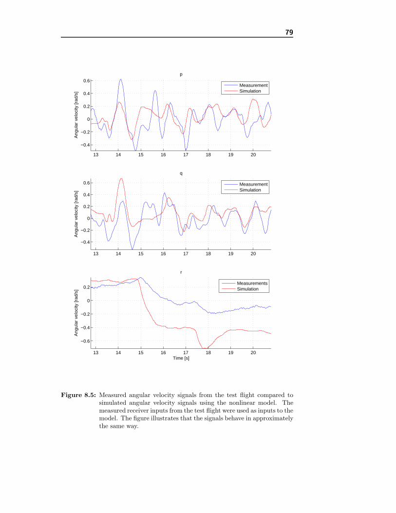
79
13 14 15 16 17 18 19 20
−0.4
−0.2
0
0.2
0.4
0.6p
Ang
ular
vel
ocity
[rad
/s]
MeasurementSimulation
13 14 15 16 17 18 19 20
−0.4
−0.2
0
0.2
0.4
0.6
q
Ang
ular
vel
ocity
[rad
/s]
MeasurementSimulation
13 14 15 16 17 18 19 20
−0.6
−0.4
−0.2
0
0.2
Time [s]
Ang
ular
vel
ocity
[rad
/s]
r
MeasurementsSimulation
Figure 8.5: Measured angular velocity signals from the test flight compared tosimulated angular velocity signals using the nonlinear model. Themeasured receiver inputs from the test flight were used as inputs to themodel. The figure illustrates that the signals behave in approximatelythe same way.

80 Flight test and model validation
in the helicopter is hard to assess without it being stable enough for a stepresponse. Improvements on the control algorithm used to regulate the he-licopter and better control on the data transmission are needed before themodel validation can be confirmed.

Chapter 9
Conclusion
The main goal with this project was to construct a four rotor helicoptercontrol system for an indoor flight. The platform for the helicopter was acustom made helicopter frame to improve sensor performance using efficientbrushless motors to induce thrust. A nonlinear dynamic model of the he-licopter was derived and a LQ regulator was designed from the linearizeddynamic model. The flight control was realized using an on-board micropro-cessor which was programmed to run pilot augmented flight control routine.Data was collected through a wireless Bluetooth connection.
9.1 Conclusion on the helicopter construction
The construction of the helicopter was discussed in chapter 3 and in appendixG. Considerable amount of time was used to make a simple, stiff and strongplatform for the four rotor helicopter.
The helicopter frameThe initial result was a simple cross with the rotors attached on each end.It was discovered that the carbon profiles used in the construction could nottolerate twisting torque repeatedly applied to them while flying. When theframe had been stiffened by attaching thin carbon fiber stripes between themotors this problem was resolved. The result is a frame that has inheritedthe specific stiffness of the carbon fiber. This is thought to minimize thestate noise derived from the flexibility of the frame in the system.

82 Conclusion
The rotorsUsing the chosen brushless DC motors combined with the chosen rotor bladesgives very good thrust to weight ratio. At hover the duty cycle is about 0.35which means that the helicopter should be able to carry a maximum payloadof about its own weight or more without going to the limit of the maximummotor current. The figure of merit for the rotors found to be 0.34 whichseems low, but the theory applied in these calculations derives from fullscale helicopters.
The flight controllerThe flight controller did not perform as well as was intended using float-ing point values for all the variables. The controller loop was running withabout 0.04[s] (25[Hz]) intervals while the integration from angular velocityto angles was done with a much smaller sample time. This was caused bythe microprocessors inability to process floating point values fast enoughto ensure high enough control loop frequency. The helicopter could not bestabilized using sample time of 0.04[s] either. Using fixed point calculationsin stead brought the control loop time under 0.010[s] (100[Hz]) which sim-ulations suggested to be small enough sample time. This however could notbe confirmed on the helicopter because of a hardware fault and the lack oftime.
The serial data connectionUsing the Bluetooth module to collect data from the helicopter was a success.It was easy to set up and worked immediately. Errors while sending the datacan however occur so that in order to get reliable data it should be packedwith some sort of error detection before sending it.
9.2 Conclusion on the controller design and simu-
lations
A linearized model of the helicopter was derived in order to design a LQregulator. The simulations show that the attitude controller stabilizes themodel with a settling time with about 1[s] which is within the specifications.
Simulations on the discrete controller that were based on the continuouscontroller showed that even with a sampling time of 0.02[s] the controllerwas able to stabilize the system, and its settling time was about the sameas for the continuous controller. There was more overshoot though. Highersampling times than 0.020[s] are not recommended because the helicopterhas small time constants and its harder to make such controllers work on

9.3 Conclusion on the validation of the nonlinear dynamic model 83
the physical system than in simulations. This is mainly because un-modeleddynamics of the system could destabilize it.
9.3 Conclusion on the validation of the nonlinear
dynamic model
Data from one of the early test flights were used to validate the nonlinearmodel. At the time of the test, the helicopter flight routines were not beingexecuted as intended resulting in a sub optimal flight performance. How-ever, the simulations using the test flight data indicate that the model canbe validated on the basis of these data. There are though some differencesthat have to be explained before the validation can be confirmed. The mostlikely explanation is the unacceptable performance of the flight controllerroutine which also can cause the data collected to be inaccurately sent viathe Bluetooth connection.
The project is considered to have been solved successfully in the sense thatthe helicopter can be flown by a pilot and the stabilizing controller worksproperly. Also the model has partly been validated even though more testsare required to confirm this.
It seems reasonable to assume that the drift of the helicopter could be stabi-lized considerably by improving the flight controller code. It is unacceptableto run a control loop at varying and too slow sample time. In order to dothis a possible solution would be to choose a microprocessor that does notlimit the capabilities of the control loop running as a real time system atthe desired sample rate.
Thorhallur Tomas Buchholz (s973637)
Dagur Gretarsson (s021235)

84 Conclusion

Bibliography
[1] Matlab and simulink. http : //www.mathworks.com/.
[2] Marcelo Alonso and Edward J. Finn. Fundamental University Physics.Volume one. Mechanics and thermodynamics. Addison-Wesley Publish-ing Company, 1980.
[3] AUCS. Areal unmanned compact system. http : //www.aucs.dk.
[4] Allan Bertelsen and Sigurjon Magnusson. Modeling and control of a4-rotor helicopter. Master’s thesis, DTU, March 2004.
[5] Bosch. Bmp085. http : //www.bosch − sensortec.com.
[6] A. R. S. Bramwell. Helicopter Dynamics. Edward Arnold, 25 Hill St.London W1X 8LL, 1976.
[7] Gunnar Christiansen, Erik Both, and Preben Østergaard Sørensen.Mekanik. Institut for Fysik, Danmarks Tekniske Universitet, 2000.
[8] University of Cambridge. Department of engineering. Interactive charts.http : //www−materials.eng.cam.ac.uk/mpsite/interactive charts/.
[9] Analog Devices. Adis16350. http : //www.analog.com.
[10] Analog Devices. Adxrs150. http : //www.analog.com.
[11] Draganfly. Draganflyer. http : //www.rctoys.com.
[12] Ericsson. Introduction of high-speed data in gsm/gprs networks. http ://www.ericsson.com/solutions.
[13] Hannu Koivisto et al. Bluetooth and wirelesslan applicability for real-time control. http ://ae.tut.f i/research/AIN/Publications/automaatio03 paper vladimir lucan−final.pdf .

86 BIBLIOGRAPHY
[14] Exitgames. Third generation mobile system. http ://www.exitgames.com.
[15] Free2move. Bluetooth module. http : //www.free2move.se.
[16] Robert A. Granger. Fluid Mechanics. Dover Publications, Inc., 1995.
[17] Graupner. Lithium ion battery. http : //www.graupner.com.
[18] Elbert Hendricks, Ole Jannerup, and Paul Haase Sørensen. LinearSystems Control. Polyteknisk, 3. edition, 2004.
[19] Gabriel M. Hoffmann, Haomiao Huang, Steven L. Waslander, andClaire J. Tomlin. Quadrotor helicopter flight dynamics and control:Theory and experiment. AIAA Guidance, Navigation and Control Con-ference and Exhibit, August 2007.
[20] IEEE. Wireless lan. http : //standards.ieee.org/getieee802/download/802.11g−2003.pdf .
[21] Ole Jannerup. Vidergaaende Styreteknik - notes 1, 3, 4, 5. Institute forautomation, DTH, February 1988.
[22] Ole Jannerup and Paul Haase Sørensen. Reguleringsteknik. DTU -Automation, 2006.
[23] Bjarne Chr. Jensen. Teknisk Stabi. Nyt Teknisk Forlag, 19 edition,2006.
[24] J. R. Hendershot Jr and Tje Miller. Design Of Brushless Permanent-Magnet Motors. Magna Physics Pub, 1994.
[25] J.Gordon Leishman. Principles of Helicopter Aerodynamics. CambridgeUniversity Press, second edition edition, 2006.
[26] Nils Leth. Servomekanismer - bind 1. Servolaboratoriet, 1978.
[27] Maxxprod. Rotor blades. http : //www.maxxprod.com/mpi/mpi −29a.html.
[28] Mikrokopter. Brushless speed controller. http ://www.mikrokopter.de/ucwiki/en/BrushlessCtrl.
[29] Eryk Brian Nice. Design of a hovering four rotor vehicle. Master’sthesis, Cornell University, May 2004.
[30] Philips. The i2c-bus specification. http ://www.nxp.com/acrobatdownload/literature/9398/39340011.pdf .

BIBLIOGRAPHY 87
[31] P. Pounds, R. Mahony, P. Hynes, and J. Roberts. Design of a fourrotor aerial robot. Proc. 2002 Australian Conference on Robotics andAutomation, 2002.
[32] Robbe. Robbe roxxy bl motors. http : //cms.robbe.com/en/.
[33] Marcel J. Sidi. Spacecraft Dynamics and control. A practical engineeringapproach. Cambridge University Press, 1997.
[34] Techworld. Zigbee. http : //www.techworld.com/mobility/features.
[35] Vishay. Fast infrared transceiver module. http ://www.vishay.com/docs/81211/tfdu6103.pdf .
[36] Neta Weiss. Understanding egprs. http ://www.comsysmobile.com/pdf/UnderstandingEGPRS.pdf .

88 BIBLIOGRAPHY

Appendix A
Rotating frame of reference
In order for Newton’s second law to work for mass moving with a non-inertialframe of reference, fictitious forces acting on it have to be introduced. Theseforces are added to the existing natural forces acting on the mass.In the following, a term for describing Newton’s second law for a movingframe of reference is derived, see (7, p.6-6).
Figure A.1: The moving system S′ turns with the angular velocity ω while O′
has the acceleration a0 relative to the inertial system S. The primesare used to mark the variables that are related to the moving frameof reference.

90 Rotating frame of reference
Figure A.1 shows the inertial system S with O as its center and the movingsystem S′ with O′ as its center. The variables related to the moving sys-tem are marked with primes. If S and S′ have the same starting point att = 0, r0 = v0t where v0 is the constant velocity of O′. At the time t theparticle P is located at r in S and at r′ in S′. The angular velocity of S′ is ω.
For an observer in S equations A.1 show r, v and a.
r = xex + yey + zez
v = dxdt ex + dy
dt ey + dzdt ez
a = dvxdt ex + dvy
dt ey + dvzdt ez
(A.1)
Equally for S′ equations A.2 show r′, v′ and a′.
r′ = x′e′x + y′e′y + z′e′z
v′ = dx′dt e
′x + dy′
dt e′y + dz′
dt e′z
a′ = d2v′xdt2
e′x + d2v′ydt2
e′y + d2v′zdt2
e′z
(A.2)
It should be noted that because the unit vectors for the moving system areconstantly changing their orientation, v′ = dr′
dt and a′ = dv′dt .
As r = r0 + r′, drdt can be expressed like in equation A.3.
dr
dt=dr0dt
+dr′
dt(A.3)
The first term on the right hand side is v0 and the second term is shown inA.4.
dr′
dt=dx′
dte′x +
dy′
dte′y +
dz′
dte′z + x′
de′xdt
+ y′de′ydt
+ z′de′zdt
(A.4)
The first three terms on the right side in equation A.4 are v′. For the lastthree terms it should be noted that the unit vectors for S′ are rotating withthe angular velocity ω and their lengths are constant. Equation A.5 showsthe term for the three unit vectors in S′ differentiated.
de′xdt
= ω × e′x,de′ydt
= ω × e′y,de′zdt
= ω × e′z (A.5)
Equation A.4 can therefore be written like A.6.

91
dr′
dt= v′ + ω × (x′e′x + y′e′y + z′e′z) (A.6)
Combining equation A.1 and equation A.6 gives A.7.
dr′
dt= v′ + ω × r′ (A.7)
Equation A.3 can therefore be written like A.8.
v = (v0 + ω × r′) + v′ (A.8)
The term inside the parentheses in A.8 is the velocity of the particle P as ifit were at rest in S′. The term v′ is the velocity of S′ relative to P .
Differentiating v in A.8 with respect to time gives A.9.
dv
dt=dv0dt
+d(ω × r′)
dt+dv′
dt(A.9)
In A.9 dvdt = a and dv0
dt = a0. Applying Newton’s second law to A.9 givesA.10.
ma = ma0 +md(ω × r′)
dt+m
dv′
dt(A.10)
The third term on the right in A.10 is shown in A.11,
mdv′dt = m(dv
′xdt e
′x + dv′y
dt e′y + dv′z
dt e′z + v′x
de′xdt + v′y
de′ydt + v′z
de′zdt ) ⇒
mdv′dt = m(a′ + ω × (v′xe′x + v′ye′y + v′ze′z))
(A.11)
or as shown in A.12.
F = mdv′
dt= m(a′ + ω × v′) (A.12)
This equation shows the forces acting on S′ relative to P .

92 Rotating frame of reference

Appendix B
Equations of angular motion
Two general equations are used to describe the dynamics of a particle in amoving frame of reference. One describes the forces acting on it (see in ap-pendix A) and the other, describing the angular momentum, or the torque,acting on it, is introduced in this chapter.
The term for moment of inertia that can be applied in the general caseof moving reference frame, called the inertia tensor, is also introduced inthis chapter.
B.1 Torque
The impulse p of a particle is shown in B.1. It is equal to the change ofmomentum for a particle (2, p.186).
p = mv (B.1)
The term for angular momentum L0 of a particle with the impulse p withrespect O is B.2 (7, p.5-2).
L0 = r × p = mr × v (B.2)
Figure B.1 shows a circular motion of a particle in a plane. With the radius

94 Equations of angular motion
Figure B.1: A particle moving in plane around a fixed point 0. The angularmomentum L0 is perpendicular to both r and v.
r, angular velocity ω and the mass m, the angular moment is B.3. Here L0
is a vector product of r and p.
L0 = mr2ω (B.3)
As the particle is moving in a circular motion around the fixed point 0, B.3can be written like B.4 (7, p.7-9).
L0 = Iω (B.4)
Here I is the moment of inertia for the point mass of the particle timesradius squared, mr2.Differentiation of B.2 gives B.5.
dL0
dt=d(r × p)
dt=dr
dt× p+ r × dp
dt(B.5)
By Newton’s second law dpdt = F and using dr
dt = v and p = mv equation B.5can be modified to B.6.
dL0
dt= v ×mv + r × F (B.6)
In B.6 the first term on the right hand side is zero because v × v = 0. Thesecond term on the right hand side is the torque, see B.7,
τ0 = r × F (B.7)

B.2 Inertia tensor 95
or B.8.
dL0
dt= τ0 (B.8)
Equation B.7 shows that the torque τ0 is a vector product of r and F . Thetorque is therefore perpendicular to the plane of the circular motion aroundthe fixed point 0.
Generally the axis of the coordinate system are moving. It is thereforenecessary to apply equation A.7, see (6, p.12), to give B.9.
dL′0
dt= Γ′ + Ω× L′
0 (B.9)
This general form of the torque can be used to describe the torques actingon a mass in a moving frame of reference.
B.2 Inertia tensor
In order to find the impulse moment L0 of a stiff body with respect to 0, itis important to know the moment of inertia for that body. This is the topicof this section.
For the orthonormal set of unit vectors, e1, e2 and e3, the impulse mo-ment L0 can be described like in B.10 (7, p.8-1).
L0 = I1ω1e1 + I2ω2e2 + I3ω3e3 (B.10)
The axes the unit vectors e1, e2 and e3 lie in, are called the principal axes.The moments of inertia in B.10 are thus called the principal moments ofinertia. Figure B.2 shows mi’s contribution Li,0 to L0. This is shown inB.11.
Li,0 = ri × pi = miri × (ω × ri) (B.11)
By inserting a orthonormal coordinate system with its center in 0 andthe unit vectors ex, ey and ez, ri can be written as (xi, yi, zi) and ω as(ωx, ωy, ωz). The vector product ω × ri can than be written as B.12.
ω × ri = (ziωy − yiωz, xiωz − ziωx, yiωx − xiωy) (B.12)

96 Equations of angular motion
Figure B.2: The mass mi’s contribution Li,0 contribution to L0.
Li,0 can be found in the same way, by the vector product of miri and ω× ri,see B.13.
Li,0 = exmi (y2i + z2
i )ωx − xiyiωy − xiziωz + eymi −yixiωx + (x2
i + z2i )ωy − yiziωz
+ ezmi −zixiωx − ziyiωy + (x2i + y2
i )ωz(B.13)
By summing all mi, the impulse moment L0 with respect to 0 can be writtenlike B.14. ⎡
⎣LxLyLz
⎤⎦ =
⎡⎣ Ixx −Dxy −Dxz
−Dyx Iyy −Dyz
−Dzx −Dzy Izz
⎤⎦
⎡⎣ωxωyωz
⎤⎦ (B.14)
The first matrix on the right hand side is called the inertia tensor I. Theindividual terms of I are shown in B.15.
Dxy = Dyx =∑mixiyi, Dxz = Dzx =
∑mixizi, Dyz = Dzy =
∑miyizi
Ixx =∑mi(y2
i + z2i ), Iyy =
∑mi(x2
i + z2i ), Izz =
∑mi(x2
i + y2i )
(B.15)

B.2 Inertia tensor 97
The upper terms in B.15 are called the products of inertia. The lower termsare the moments of inertia. Equation B.14 can now be written like B.16.
L′0 = IΩ (B.16)
If the coordinate system, with which the stiff body is moving, can be turnedso that 0 lies in the body’s center of mass and the body is symmetricalaround all the axes, then B.14 can be simplified to B.17, see (7, p.8-3) and(6, p.15). ⎡
⎣LxLyLz
⎤⎦ =
⎡⎣Ixx 0 0
0 Iyy 00 0 Izz
⎤⎦
⎡⎣ωxωyωz
⎤⎦ (B.17)

98 Equations of angular motion

Appendix C
Euler angle rotation
The projection between two coordinate systems, inertial frame coordinatesand moving frame coordinates is the topic of this chapter.
A successive angular rotation about the three orthogonal frame axes is calledthe Euler angle rotation. Out of the six possible ways this can be done, onlyone will be introduced here, see (33, p.320).
It is common to define the Euler roll angle φ as the rotation about thebody’s x axis, the pitch angle θ about the y axis and the yaw angle ψ aboutthe z axis.
By assuming that initially the moving frame axes are aligned with the axesof the initial frame, transformation ψ → θ → φ is done in the following way:
Rotating about the z axes is the first step. It is done with the transfor-mation matrix seen in C.1.
⎡⎣x1
y1
z1
⎤⎦ =
⎡⎣ cos(ψ) sin(ψ) 0−sin(ψ) cos(ψ) 0
0 0 1
⎤⎦
⎡⎣XYZ
⎤⎦ =
[Aψ
] ⎡⎣XYZ
⎤⎦ (C.1)
Initially, the body axes were aligned with the reference axes X, Y and Z.
The next step is to rotate about the y axis. That is done with the rota-tional matrix seen in C.2.

100 Euler angle rotation
⎡⎣x2
y2
z2
⎤⎦ =
⎡⎣cos(θ) 0 −sin(θ)
0 1 0sin(θ) 0 cos(θ)
⎤⎦
⎡⎣x1
y1
z1
⎤⎦ =
[Aθ
] ⎡⎣x1
y1
z1
⎤⎦ (C.2)
The last rotation is about the x axis. The rotational matrix can be seen inC.3. ⎡
⎣x3
y3
z3
⎤⎦ =
⎡⎣1 0 00 cos(φ) sin(φ)0 −sin(φ) cos(φ)
⎤⎦
⎡⎣x2
y2
z2
⎤⎦ =
[Aφ
] ⎡⎣x2
y2
z2
⎤⎦ (C.3)
This results in C.4.⎡⎣xyz
⎤⎦ =
⎡⎣x3
y3
z3
⎤⎦ =
[Aφ
] [Aθ
] [Aψ
] ⎡⎣XYZ
⎤⎦ =
[Aψθφ
] ⎡⎣XYZ
⎤⎦ (C.4)
The projection matrix can be seen in C.5.
[Aψθφ
]=
⎡⎣ c(θ)c(ψ) c(θ)s(ψ) −s(θ)−c(φ)s(ψ) + s(φ)s(θ)c(ψ) c(φ)c(ψ) + s(φ)s(θ)s(ψ) s(φ)c(θ)s(φ)s(ψ) + c(φ)s(θ)c(ψ) −s(φ)c(ψ) + c(φ)s(θ)s(ψ) c(φ)c(θ)
⎤⎦
(C.5)
For convenience c(...) in C.5 means cos(...) and s(...) means sin(...).
The projection from the moving frame coordinates into the inertial framecoordinates are done with the transposed matrix [Aψθφ]T , see (33, p.319).The transposed matrix can be seen in C.6.
[Aψθφ
]T =
⎡⎣c(θ)c(ψ) −c(φ)s(ψ) + s(φ)s(θ)c(ψ) s(φ)s(ψ) + c(φ)s(θ)c(ψ)c(θ)s(ψ) c(φ)c(ψ) + s(φ)s(θ)s(ψ) −s(φ)c(ψ) + c(φ)s(θ)s(ψ)−s(θ) s(φ)c(θ) c(φ)c(θ)
⎤⎦
(C.6)

Appendix D
Thrust and H-force
D.1 Rotor thrust
The theoretical thrust produced by a rotor in forward flight can be seen inequation (D.1), (6, p.147).
T = ρσArΩ2rR
2r
a
4
[23θ0(1 +
3µ2
2) + λ
](D.1)
In (D.1) ρ is the air density, Rr is the rotor radius, Ar is the rotor area andΩr is the angular velocity of the rotor. The ratio of blade lifting area anddisk area is called the rotor solidity. It can be seen in (D.2). Here b is thenumber of rotor blades and c is the blade chord at 3
4Rr.
σ =Blade area
Disk area=AbAr
=bcRrπR2
r
=bc
πRr(D.2)
The thrust coefficient of equation (D.1), CT can be seen in (D.3).
CT =a
4
[23θ0(1 +
3µ2
2) + λ
](D.3)
In (D.3), a represents the lift-curve slope of the airfoil section (25, p.119).The effective pitch angle of the rotor blade is θ0.
Equation (D.4) shows the tip speed ratio.

102 Thrust and H-force
µ =
√v2 + u2 + w2 cos(argtan w√
v2+u2)
ΩrRr(D.4)
The disk plane inflow velocity λ can be seen in equation (D.5).
λ =sin(AWU)
ΩrRr− λi (D.5)
AWU from (D.5) depends on u and w. The relationship can be seen inequation (D.6), (4, 106).
AWU =
⎧⎪⎪⎪⎨⎪⎪⎪⎩
if u > 0, w > 0 then arg tan( w√u2+v2
)if u > 0, w < 0 then arg tan( w√
u2+v2)
if u < 0, w > 0 then − arg tan( w√u2+v2
)if u < 0, w < 0 then − arg tan( w√
u2+v2)
⎫⎪⎪⎪⎬⎪⎪⎪⎭
(D.6)
From (D.5) λi can be written like equation (D.7) (4, p. 106).
λi = 0.047√
−226.35µ2 +√
226.352µ4 + 1 (D.7)
D.2 H-force
The H-force of a rotor is described by (D.8).
Hr = ρsArΩ2rR
2r [
14µδ − a
4λDµθ0] (D.8)
In equation (D.8), δ = 0.012 (4, 106) is the profile drag coefficient. All othervalues have been described above.

Appendix E
The inertia of the helicopter
The inertia of the helicopter can be described in an inertia tensor as shownin appendix B. The inertia tensor shows the inertia about the three princi-pal axes.
As the helicopter is an irregular object, it would be much work to approxi-mate its inertia. Instead the inertia about the three principal axes has beenmeasured.
Figure E.1 shows the setup for the measurement. By using a spring witha known spring constant attached to a rigid support, the helicopter can betreated like a torsion pendulum with suspending it to the spring. The periodtime of the harmonic motion this rotation follows when rotated and releasedis measured and used to calculate the inertia about the respective axis.
A spring was made of piano wire. To measure its torsion constant, a rodwith known inertia was used. Equation (E.1) shows the inertia for a rod.
Ic =112Ml2 (E.1)
In (E.1) M is the mass of the rod, and l is the length of it.
The relationship between the period time and the torsion constant is shownin equation (E.2).
T = 2π
√IcK
(E.2)
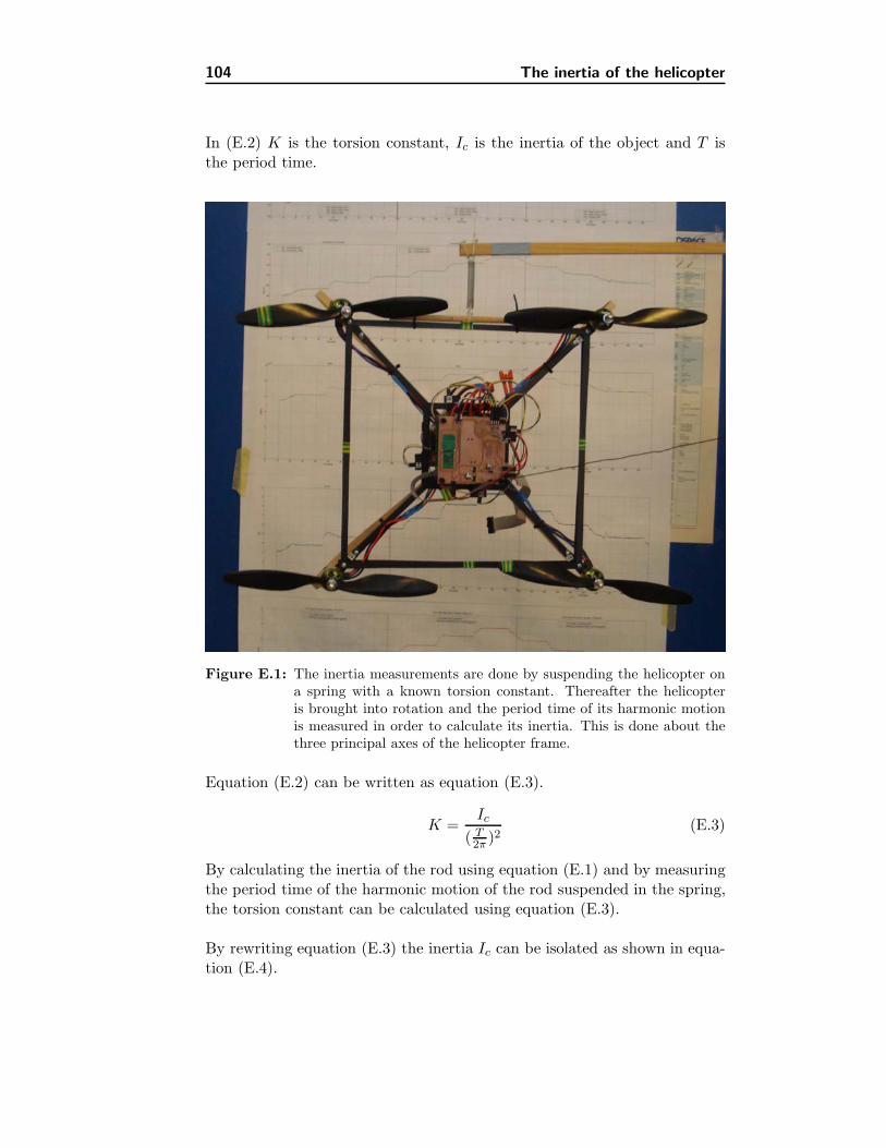
104 The inertia of the helicopter
In (E.2) K is the torsion constant, Ic is the inertia of the object and T isthe period time.
Figure E.1: The inertia measurements are done by suspending the helicopter ona spring with a known torsion constant. Thereafter the helicopteris brought into rotation and the period time of its harmonic motionis measured in order to calculate its inertia. This is done about thethree principal axes of the helicopter frame.
Equation (E.2) can be written as equation (E.3).
K =Ic
( T2π )2(E.3)
By calculating the inertia of the rod using equation (E.1) and by measuringthe period time of the harmonic motion of the rod suspended in the spring,the torsion constant can be calculated using equation (E.3).
By rewriting equation (E.3) the inertia Ic can be isolated as shown in equa-tion (E.4).

105
Ic = K(T
2π)2 (E.4)
By measuring the harmonic motion period time of the helicopter rotatingabout its three principal axes, equation (E.4) can be used to calculate theirrespective inertias.
The torsion constant K was measured by using a rod with l = 0.524[m]and M = 0.524[kg]. Three measured period times gave a mean period timeT = 12.05[s]. This gives the torsion constant T = 0.00326[kgm
2
s2].
The mean measured swing periods about the x, y and z axis were mea-sured 9.7[s], 9.67[s] and 14.53[s] respectively. By using equation E.4 theinertia tensor shown in equation E.5 was derived.
I =
⎡⎣Ixx 0 0
0 Iyy 00 0 Izz
⎤⎦ =
⎡⎣0.00777 0 0
0 0.00772 00 0 0.0175
⎤⎦ (E.5)
This inertia tensor is used in the simulink model.

106 The inertia of the helicopter

Appendix F
Rotor inertia
In order to calculate the spinning rotors gyro effect and the torque causedby change in angular velocity of the rotors, it is necessary to know their mo-ment of inertia about the center of rotation. To do this, one of the RoxxyRobbe motors was disassembled and the inertia of its rotating parts wasmeasured along with that of the blade.
Figure F.1 shows one of the rotors used on the helicopter.
Figure F.1: One of the helicopter rotors
To calculate approximately the rotors moment of inertia it is disassembledinto three pieces, the rotor blade, the stator and the rotor mount. Thesepieces are all irregularly shaped. Their form is therefore fitted to a regularform with known moment of inertia. These are a rod, a ring and a circularplate respectively.

108 Rotor inertia
The blade mount, see figure F.2, is approximated with a circular plate.
Figure F.2: The blade mounting. The lower part is fastened to the motor withthree screws. The blade is than fastened by tightening the nut.
Its moment of inertia can then be calculated using F.1.
I =12mr2 (F.1)
The estimated radius of the rotor mount is rm = 0.007[m] and its mass ismm = 0.005[kg]. That gives Im = 1.225e−7[kgm2]
The stator can be seen in figure F.3. It is approximated with a ring ro-tating around an axle in its center. Equation F.2 shows the formula for theinertia of a ring.
Figure F.3: The stator. Here the permanent magnets can be seen.
I = mr2 (F.2)

109
The estimated radius of the stator is rs = 0.013[m] and its mass is ms =0.018[kg]. This gives Is = 3e−6[kgm2].
A picture of the rotor blade can be seen in figure F.4. It is assumed equiva-lent to a rod rotating around an axle in its center. Equation F.3 shows theformula for the inertia of a rod.
Figure F.4: One of the rotor blades used on the helicopter.
I =112ml2 (F.3)
The length of the rotor blade is lrb = 0.254[m] and its mass is mrb =0.006[kg]. This gives Irb = 3.2e−5[kgm2]
The total inertia of the rotor is shown in F.4.
Ir = Im + Is + Irb = 3.5e−5[kgm2] (F.4)
The approximations used to calculate the moment of inertia for the rotor,are considered to give a good estimation of its true moment of inertia. Therotors moment of inertia together with its air resistance control the timeconstant of the rotor. As the time constant has been measured no attemptshave been made to measure the inertia of the rotor.

110 Rotor inertia

Appendix G
Helicopter frame construction
In this chapter, a complete construction of a four rotor helicopter platformis introduced. The goal of the construction is to build a battery poweredhelicopter that is small enough to be used for wireless indoor flight exper-iments. The helicopter is thus restricted in size which also limits the totalweight it can carry.
G.1 Frame materials
The main emphasis in choosing the materials used for the frame construc-tion is that they are lightweight, stiff, strong and easy to work with. Asthis is a prototype helicopter which is to be a platform for the design of anautonomous control system, the cost of the materials is considered to be lessimportant, as are other material features such as service temperature andwater resistance.
The construction materials considered for the frame are wood, metals, com-posite materials and polymers. Generally, materials with high specific strengthand specific stiffness are preferred in aerospace applications. Specific strengthis the strength to density ratio and the specific stiffness is the stiffness toweight ratio. Wood and polymers can therefore be ruled out immediately asthe main construction materials. These material classes have lower specificstrength than metals and composite materials and are therefore less suitablefor this application. This can be seen in figure G.1. Furthermore figure G.1shows that composite materials generally have higher specific strength than

112 Helicopter frame construction
metals or metal alloys.
Figure G.1: Material specific stiffness and specific strength ratio domains.(8)
Figure G.2 shows that the toughness of metals and composite materials aresimilar. The choice therefore, lies between these two categories.
Aluminum is the best metal candidate for this application. It is strong,stiff, light and easy to work with. The diversity of aluminum profiles on themarket is also great.
Carbon fiber reinforced polymer (CFRP) is not as easy to use and the diver-sity of profiles available for this particular application is also less. Carbonfiber, however, has higher specific strength and specific stiffness than alu-minum.
Carbon fiber is therefore selected as the main construction material of theframe. Other materials used for the frame construction are aluminum andpolyamide (nylon). This can be seen below.

G.2 Frame design 113
Figure G.2: Material strength and toughness ratio domains.(8)
G.2 Frame design
The goal of the frame design is to build a simple, light weight and stiff framewhich is strong enough to carry itself, all the electronics of the control sys-tem, the rotors and a battery with enough capacity to fly the helicopter forseveral minutes. Furthermore, the frame interference with the rotor wakesshould be minimal.
This is done by designing a horizontal cross frame with equally long armswhere one rotor is mounted on the end of each arm. The printed circuitboards and the battery are mounted in the center of the frame as payload.
G.2.1 Frame arms
The arms are constructed of CFRP tubes. When choosing between roundand square tubes the forces acting on each arm have to be taken into ac-count. Given that the arm lies parallel to the x axis, the forces acting onit are approximately perpendicular to the x − y plane and x− z plane, seechapter 2.

114 Helicopter frame construction
Figure G.3: Beam with force P [N ] acting on it. The deformation is U [m] andthe length from the one support to the other is l[m]
With this approximation the arm profile can be treated as a ordinary beamwith force acting on as shown in figure G.3.
Equation (G.1), see (23) describes the deformation U [m] as a function ofapplied force P [N ], length l[m], Young’s modulus E[ N
m2 ], which is a mea-sure of stiffness, and the second moment of inertia I[m4] which is a crosssectional parameter.
U =148Pl3
EI(G.1)
For two beams made of the same material, the only variable parameter is theinertia I. For a beam made of square tube with equal sides as and materialthickness ds, the inertia is described with equation (G.2).
Is =112
(a4s − (as − 2ds)4) (G.2)
For a beam made of round tube with the outer diameter ar and materialthickness dr the inertia is described with equation (G.3).
Ir =π
64(a4r − (ar − 2dr)4) (G.3)
Assuming that the inertia of the two beams is the same and ab = ar = as,equations (G.2) and (G.3) can be combined and solved for dr as a functionof ds, see equation (G.4).

G.2 Frame design 115
dr =ab − (ab −
6412
(a4b−(ab−2ds)4)
π )14
2(G.4)
The mass of the square and the round tubes can be seen in (G.5) and (G.6)respectively.
ms = Vsρ = Aslsρ = (a2s − (as − 2ds)2)lsρ (G.5)
mr = Vrρ = Arlrρ = (π(ar2
)2 − π(ar2
− dr)2)lrρ (G.6)
For the two beams, the material density, ρ, and the beam length, l, are thesame. The difference in mass is thus only dependent on the difference in thecross sectional area of the two beams.Two equally long and broad square tube and round tube beams are com-pared in table G.1. It shows that in order to be equally stiff, the crosssectional area of the round tube has to be 60.2% higher than that of thesquare tube.
- a[m] d[m] I[m4] A[m2]Square tube 0.008 0.000600 1.6316 ∗ 10−10 1.776 ∗ 10−5
Round tube 0.008 0.001364 1.6316 ∗ 10−10 2.844 ∗ 10−5
Table G.1: Square tubes and round tubes compared.
For the square tube selected, see below, with the dimensions a = 0.008[m]and d = 0.0006[m], the density ρ is measured to be 1406[ kg
m3 ]. With thelength of the four tubes attached to the cross, see below, l = 0.215[m] themass of the four tubes is ms = 0.0215[kg]. By using equally stiff and broadround tubes this mass would be mr = 0.0344[kg].
To determine the Young’s modulus E[ Nm2 ] of the square arms chosen, the
setup in figure G.3 was used, see figure G.4. In this test, the l = 0.8[m],m = 1.355[kg] and U = 0.00954[m]. The second moment of inertia can beseen in table G.1. The Young’s modulus is calculated E = 91.14[GPa]. Thespecific stiffness of the beam is E
ρ = 64.8[MNmkg ] which falls within the CFRP
domain shown in figure G.1.
Another big advantage of the square tubes is, that their flat surface makesthe mounting of peripherals such as the rotors much easier.

116 Helicopter frame construction
Figure G.4: The square beam with a mass stressing it.
G.2.2 Center cross
The function of the center cross is twofold. It is used to join the arm profilestogether in a cross (see figure G.6), and it is used as a support inside thesquare profiles so that they do not collapse when the printed circuit boards(PCB) and battery are attached to the frame with screws, see figure G.5.The arms slide up on the center cross and are glued to it with epoxy glue.
Figure G.5: A section of a CFRP profile with a piece of nylon inside it for support.The nylon supports the profile so that it does not collapse whenscrews are used to mount something on it.
The material chosen for the center cross is nylon. It is light weight and itseasy to work with. The strength and stiffness of the center cross are moretrivial, partly because it is surrounded by the arms but also because the

G.2 Frame design 117
Figure G.6: The center cross is used to join the arms and act as support withinthe profiles when something has to be fastened to the frame withscrews.
center plate, see below, ensures its stiffness. The weakness of this construc-tion lies in the center where the nylon does not have any support from thecarbon fiber. This is solved by adding center plates to the construction.
G.2.3 Center plates
The purpose of the center plates, see figure G.7, is to stiffen the frame to agreater extent. They are made of CFRP.
Figure G.7: Center plate
When these are glued with epoxy on top and beneath the center of theframe, it connects the arms on the opposite side of the center and alsocovers the otherwise exposed nylon in the center. This creates sort of asandwich construction in the sense that it adds a very strong outer shell tothe nylon core that is not nearly as stiff. The center plates also stiffens theside movements of the arms with the cross beam between them. In addition

118 Helicopter frame construction
to the glue, the center plates are held in place by the screws supporting thePCB platform.
G.2.4 Rotor mountings
Attaching the rotors to the helicopter is done with the mounting brackets,see figure G.8, fastened to the end of the arms with glue and two 3[mm] ny-lon bolts. The rotor mounts are made of aluminum, partly because CFRPis harder to work with and partially because nylon is not as stiff. When itis screwed on the surface of the arm, square pieces of nylon are slid into toend of the frame as support so that the profiles do not collapse, see figureG.5. The nylon bolts holding the mounts are also used to fasten the landingframe, see section G.3.
Figure G.8: The rotor mounting is made of aluminum.
G.2.5 Frame extra supports
After the construction of the frame, one weakness was discovered. Whena twisting torque is applied to the carbon fiber square profiles they caneasily begin to crack lengthwise along the profiles. This weakens the profilestructure considerably. The reason for this is, that the profiles are only madeof one layer of fibers that lie lengthwise. If the profiles were fabricated byusing two layer of fibers crossing each other this would not be a problem.Attempts to come across better fabricated profiles suitable for the framewere not successful. Extra supports were therefore added to the frame.These are narrow carbon fiber bands connecting the end of the arms, seefigure G.9.

G.3 Landing frame 119
G.3 Landing frame
The landing frame is made of thin stripes of ash wood. These can be seenon figure 3.3. The ash wood light weight and very flexible. It can thereforeeasily be bent into shape. Alternatively some plastic stripes can be used.The landing gear is made flexible enough to be able to absorb the energy tosome extent when the helicopter crash lands and thereby protects the framefrom being damaged. At the same time, the landing frame has to be stiffenough to keep the helicopter from vibrating uncontrollably when taking off.
G.4 The helicopter frame
The assembled helicopter frame can be seen in figure G.9.
Figure G.9: The complete frame of the helicopter. The landing frame is not shownhere.
By constructing the frame in this way, the high specific stiffness of the squaretubes was retained. The mass of the whole frame is m = 0.075[kg] which isless than the mass of one rotor (m = 0.075[kg]). The frame is only about10% of the helicopters total mass which is m = 0.744[kg].
G.5 Frame drag
In order to calculate the drag force of the helicopter, the frontal area has tobe known. This will be treated here.
The frontal area of the helicopter depends on the relative direction it isflying. The largest frontal area is therefore estimated here. As its shape isirregular, some approximations have to be made.

120 Helicopter frame construction
In the following, the helicopter is split into four area parts, the motors,the frame, the printed circuit boards and the battery.
The four motors are all approximated to be 0.025[m] by 0.025[m] squares.The cross sectional area of the motors is Am = 0.000625[m2 ].
The frame is 0.436[m] by 0.006[m]. The frontal are of the frame is thusAm = 0.002616[m2 ].
The printed circuit boards with all the electronic are 0.10[m] by 0.055[m]which gives Ac = 0.0055[m2].
The battery is 0.08[m] by 0.02[m] which gives Ab = 0.0016[m2 ].
The combined frontal area of the helicopter is thus Af = 0.0103[m2].
The largest frontal area of the helicopter Af can now be used to calculatethe drag force acting on it in flight, see chapter 4.2.1.

Appendix H
The single chip yaw rate gyroADXRS150
In this appendix tests of gyroscopes, yaw rate gyro ADXRS150 (10), that areused to measure the attitude of the four rotor helicopter, are made. Thesemeasurements are done to evaluate the drift of the gyroscopes.
Test of a single chip yaw rate gyro, ADXRS150 by Analog Devices, weredone by sampling the outputs of the gyroscope, with the helicopter sittingstationary on the floor. Sampling is done with the microprocessor on theflight controller board and the data is sent by Bluetooth to a computer whereMatlab logs the data. Further information for the gyroscopes can be seenin (10).
Steady state test of gyroscopes
The gyroscope has a sensitivity of ±150[/s] @ 25C or 2.618[rad/s] andthe data was logged over 900 seconds with interval of 31.6ms. In figureH.1, the logged angular velocity is plotted in rad/s. The angular velocityaround the x-axis is psensor, the angular velocity around the y-axis is qsensorand the angular velocity around the z-axis is rsensor. The mean value ofthe measurements was subtracted from each sample to eliminate offset. Thestandard deviation, σ, for the steady state measurement are shown in tableH.1.
By integrating the angular speed, angular drift is obtained. is presented in

122 The single chip yaw rate gyro ADXRS150
0 100 200 300 400 500 600 700 800 900−0.02
−0.01
0
0.01
0.02Angular speed
p sens
or [r
ad/s
]
Time [s]
0 100 200 300 400 500 600 700 800 900−0.02
−0.01
0
0.01
0.02
q sens
or [r
ad/s
]
Time [s]
0 100 200 300 400 500 600 700 800 900−0.05
0
0.05
r sens
or [r
ad/s
]
Time [s]
Figure H.1: Angular speed measurements of the gyros. Measurements are loggedover a period of 900 seconds.

123
σp = 2.67 · 10−3[rad/s]σq = 2.66 · 10−3[rad/s]σr = 4.28 · 10−3[rad/s]
Table H.1: Standard deviation for measurement in rad/s. σp is the standarddeviation for psensor , σq is the standard deviation for qsensor and σr
is the standard deviation for rsensor .
figure H.2.
The steady state measurements of the gyroscopes, show that the gyroscopesare not identical. Sensors psensor and qsensor look more alike while the rsensorhas more standard deviation. Sensor rsensor has higher noise peaks than thetwo others, while the angular drift of rsensor (ψsensor) and qsensor (θsensor)are similar. These drifts of the gyroscopes vary with change in temperature.
This means that the drift of the gyroscopes causes the four rotor helicopterto drift. The pilot of the helicopter has to counteract these effects, sincethere is no positioning measurement of the helicopter.
In H.3 the steady state measurements of the gyroscopes are displayed in his-tograms. It shows how frequently each value in the measurements appears,in ratio from 0-1.

124 The single chip yaw rate gyro ADXRS150
0 100 200 300 400 500 600 700 800 900−0.08
−0.06
−0.04
−0.02
0
0.02Angle
φ sens
or [r
ad]
Time [s]
0 100 200 300 400 500 600 700 800 900−0.1
0
0.1
0.2
0.3
θ sens
or [r
ad]
Time [s]
0 100 200 300 400 500 600 700 800 900−0.05
0
0.05
0.1
0.15
0.2
ψse
nsor
[rad
]
Time [s]
Figure H.2: Calculated angles of the angular speed measurements over period of900 seconds.

125
−0.015 −0.01 −0.005 0 0.005 0.01 0.0150
0.05
0.1
0.15
0.2
0.25
PDF for psensor
[rad/s]
−0.015 −0.01 −0.005 0 0.005 0.01 0.0150
0.1
0.2
0.3
0.4
PDF for qsensor
[rad/s]
−0.06 −0.04 −0.02 0 0.02 0.04 0.060
0.05
0.1
0.15
0.2
0.25
PDF for rsensor
[rad/s]
Figure H.3: Probability density function for the gyroscopes steady state measure-ments.

126 The single chip yaw rate gyro ADXRS150

Appendix I
Rotor measurements
In this chapter the results from rotor measurements are presented. Threerotor blades were measured and compared. The chosen rotor blade is shownin section I.2 and the two other blades are shown in section I.3.
The measurements show the relationship between duty cycle, angular veloc-ity, thrust and torque of the rotors. The results from these measurementsare used to generate functions that are used in the Matlab/Simulink modelof the helicopter.
I.1 Measurement setup
The measurement setup is shown in figure I.1. The rotor blades are attacheddirectly to the motor and the motor is controlled by the controller. Thecontroller gets a PWM signal from an Atmel development board STK500with the Atmega 128 microprocessor and is powered by an 11[V ] powersupply. By varying the duty cycle into the controller, different angularfrequencies are obtained.
The angular frequency of the rotor is measured with a reflective object sen-sor, OPB 701, placed under the rotor blades beside the motor. The sensorcan be seen in figure I.2. The angular velocity is calculated as half of themeasured angular frequency. This is because the rotor blade has to passthe sensor two times to complete one circle. The equation for the angularvelocity passing the sensor two times is:

128 Rotor measurements
Figure I.1: Measurement setup.
ωr = 2πf/2.
The rod, to which the motor and reflective object sensor are fastened, standson a weight scale, see figure I.3.
Figure I.2: Angular velocity measurements are done with reflective object sensor,OPB 701.
Thrust measurements are made with the scale and are measured in grams.The scale is a top loading Philips HR 2385/A with the accuracy of ±1g .Thrust in newtons is calculated using Newton’s second law,
F = m · a
Where m[kg] is the weight measured by the scale and a[m/s2] is the earthgravity. Torque measurements are done using a turntable and a weightscale, see figure I.4. The turntable is put on the side, placing the rotor onthe middle. A rod connects the turntable to the scale.

I.1 Measurement setup 129
Figure I.3: Thrust measurements, with scale.
Figure I.4: The torque measurement setup.

130 Rotor measurements
The torque τ [Nm] is calculated using equation:
τ = m · l · g
Where m[kg] is the mass measured by the scale, l[m] is the length from themiddle of the turntable to the rode attached to the scale and g[m/s2] is theearth gravity.
I.2 Applied rotor blades
In this section the measurements of the rotor blades used for the four rotorhelicopter are presented. The length of the blades is 254[mm] which is lessthan for the other two blades that were not chosen, resulting in less drag andmore angular velocity. The results are used in the Matlab/Simulink modelfor the helicopter.
I.2.1 Duty cycle and angular velocity
The relations between duty cycle and angular velocity is shown in figureI.5. These measurements are made by varying the duty cycle controllingthe rotor and measuring the angular frequency and finally calculating theangular velocity. These results are then taken and fitted using the Matlabfunction polyval. The result is a second order polynomial function shownin equation I.1
ωR1(DR1) = −838.58 ·D2R1 + 1545.2 ·DR1 − 117.63
ωR2(DR2) = −724.67 ·D2R2 + 1418.0 ·DR1 − 86.696
ωR3(DR3) = −738.80 ·D2R3 + 1414.2 ·DR1 − 92.171
ωR4(DR4) = −756.91 ·D2R4 + 1363.7 ·DR1 − 49.655
(I.1)
These coefficients are used in the Matlab/Simulink model of the helicopter.
I.2.2 Angular velocity and thrust
In figure I.6 the relations between angular velocity and thrust is shown. Asmentioned in previous section the results are fitted with Matlab. In equationI.2 the results are shown.

I.2 Applied rotor blades 131
0.2 0.3 0.4 0.5 0.6 0.7 0.8 0.9200
250
300
350
400
450
500
550
600
Ang
ular
vel
ocity
[rad
/s]
Duty cycle
Duty cycle vs. angular velocity
Rotor 1Rotor 1 fitRotor 2Rotor 2 fitRotor 3Rotor 3 fitRotor 4Rotor 4 fit
Figure I.5: Duty cycle controlling the rotors is plotted against the angular velocityfor each rotor.
100 200 300 400 500 6000
1
2
3
4
5
6
Thr
ust [
N]
Angular velocity [rad/s]
Angular velocity vs. Thrust
Rotor 1Rotor 1 fitRotor 2Rotor 2 fitRotor 3Rotor 3 fitRotor 4Rotor 4 fit
Figure I.6: Angular velocity of the rotors is plotted against the thrust for eachrotor.

132 Rotor measurements
TR1(ωR1) = 15.998 · 10−6 · ω2R1 − 1.7593 · 10−3 · ωR1 + 214.05 · 10−3
TR2(ωR2) = 15.781 · 10−6 · ω2R2 − 0.9070 · 10−3 · ωR2 + 80.918 · 10−3
TR3(ωR3) = 13.375 · 10−6 · ω2R3 + 1.1213 · 10−3 · ωR3 − 193.14 · 10−3
TR4(ωR4) = 15.818 · 10−6 · ω2R4 − 0.5653 · 10−3 · ωR4 + 23.589 · 10−3
(I.2)
These coefficients are used in the Matlab/Simulink model of the helicopter.
I.2.3 Angular velocity and torque
In figure I.7 the relations between angular velocity and torque are shown.The results are fitted using Matlab resulting in equation I.3.
100 200 300 400 500 6000
0.1
0.2
0.3
0.4
0.5
0.6
0.7
Tor
que
[Nm
]
Angular velocity [rad/s]
Angular velocity vs. Torque
Rotor 1Rotor 1 fitRotor 2Rotor 2 fitRotor 3Rotor 3 fitRotor 4Rotor 4 fit
Figure I.7: Angular velocity of the rotors is plotted against the torque for eachrotor.
τR1(ωR1) = 1.5226 · 10−6 · ω2R1 + 56.190 · 10−6 · ωR1 − 14.581 · 10−3
τR2(ωR2) = 1.8526 · 10−6 · ω2R2 − 106.31 · 10−6 · ωR2 + 12.710 · 10−3
τR3(ωR3) = 1.3391 · 10−6 · ω2R3 + 267.13 · 10−6 · ωR3 − 38.838 · 10−3
τR4(ωR4) = 1.4517 · 10−6 · ω2R4 + 154.46 · 10−6 · ωR4 − 28.498 · 10−3
(I.3)
The coefficients are used in the Matlab/Simulink model of the helicopter.

I.3 Other rotor blades 133
I.3 Other rotor blades
In this section measurements for two rotor blades, not used for the four rotorhelicopter, are presented. These rotor blades are longer than the blade usedfor the helicopter. Blade 1 is 336[mm] and blade 2 is 280[mm].
I.3.1 Duty cycle versus angular velocity
Figure I.8 shows the relation between the duty cycle to the controller and theangular velocity for the two rotor blades. Blade 2 achieves higher angularvelocity than blade 1 for any given duty cycle, indicating that blade 2 hasless drag.
0.2 0.3 0.4 0.5 0.6 0.7 0.8
50
100
150
200
250
300
350
Ang
ular
vel
ocity
[rad
/s]
Duty cycle
Duty cycle for controller vs. angular velocity
Blade 1Polyfit for Blade 1Blade 2Polyfit for Blade 2
Figure I.8: Duty cycle for driver versus angular for the two rotor blades.
I.3.2 Angular velocity and thrust
The angular velocity is plotted against the thrust from the rotor blades infigure I.9. Here it can bee seen that blade 1 has more lift than blade 2 forevery given angular velocity.

134 Rotor measurements
0 50 100 150 200 250 300 350 4000
0.5
1
1.5
2
2.5
3
3.5
Thr
ust [
N]
Angular velocity [rad/s]
Angular velocity vs. Thrust
Blade 1Blade 2
Figure I.9: Angular velocity versus thrust for the two rotor blades.
I.4 Figure of merit
The figure of merit (FM) is a way to asses the rotors relative performance.It is a dimensionless number between 0 − 1 where 1 is ideal. FM has beencalculated for the rotors using the different rotor blades. The definition offigure of merit can be seen in equation I.4, (25, p. 73).
FM = Pideal/Pmeas (I.4)
Pideal is found in appendix J can be seen in the following equation I.5.
Pideal = T ∗ sqrt T
2ρA(I.5)
Here ρ is the density of air and A is the area of the rotor. Pmeas can befound with equation I.6.
Pmeas = U ∗ I (I.6)
Figure of merit was calculate to be 0.34 for the applied rotor, 0.22 for therotor using rotor blade 1 and 0.266 for rotor blade 2. These seem relativelylow, but the applied theory is used on full size helicopters rotors and it isnot sure that it can be applied to small size rotors in unchanged form.
It is clear from all the data above that the applied rotor is the best choice

I.4 Figure of merit 135
in this project. The rotor blades 1 and 2 perform much worse. It shouldthough be noted that their rotor area is much larger so they might performbetter using different motors. This is supported by the fact that they givegreater lift at lower velocities.

136 Rotor measurements

Appendix J
Momentum theory
In this chapter, a theoretical basis for a simple analysis of the rotor per-formance in hovering flight is derived. This is known as Rankine-Froudemomentum theory, (25, p.58).
In this approach, the following assumptions are made. The rotor bladesare treated as an infinitely thin disk with the area A, over which a pressuredifference exists, see figure J.1. Far upstream and downstream of the rotorthe velocity of the fluid is quiescent. Viscous effects are negligible. Thethrust loading and induced velocity are uniformly distributed over the disk.The fluid is assumed to be incompressible. Furthermore, the flow throughthe rotor is considered to be one dimensional and quasi-steady, or that theflow properties at a point do not change with time. Fluid properties onlychange with axial position relative to the rotor.
Three conservation laws now apply to the model and can be used in the fol-lowing. These are conservation of mass, momentum and energy. Referringto figure J.1, a control volume surrounding the rotor and its wake has thesurface area S. Equation J.1 describes the conservation of mass by statingthat the mass flow into the control volume is equal to the mass flow out ofit. ∫ ∫
Sρ−→V · d−→S = 0 (J.1)
The conservation of fluid momentum is described by equation J.2. Here theforce on the fluid is supplied by the rotor. Newton’s third law states that

138 Momentum theory
Figure J.1: Fluid flow model for momentum theory visualization.
the fluid exerts a counterforce on the rotor. This force is the thrust, T.
−→F =
∫ ∫Spd
−→S +
∫ ∫S(ρ−→V · d−→S )
−→V (J.2)
The work done on the fluid by the rotor is expressed in equation J.3. Itsimply states that the work done by the rotor on the fluid increases itskinetic energy.
W =∫ ∫
S
−→V 2 1
2(ρ−→V · d−→S ) (J.3)
These equations can now be used with the model shown in figure J.1, whichrepresents a hovering helicopter rotor. The area of the disk is A, the crosssection 0 represents the plane far upstream, cross sections 1 and 2 the planejust above and below the rotor disk respectively. The cross section ∞ rep-resents the plane far downstream.
The mass flow rate, equation J.4 is assumed to be constant within the bound-aries of the wake.
m =∫ ∫
∞ρ−→V · d−→S =
∫ ∫2ρ−→V · d−→S (J.4)
Equation J.4 reduces to equation J.5.

139
m = ρA∞w = ρA2vi = ρAvi (J.5)
The relationship between the thrust and the net time rate-of-change of fluidmomentum out of the wake is given by equation J.6. This is in accordancewith Newton’s second law.
−−→F = T =
∫ ∫∞ρ(−→V · d−→S )
−→V −
∫ ∫0ρ(−→V · d−→S )
−→V (J.6)
In hovering flight, the velocity of the fluid far upstream is negligible. Thesecond term on the right of equation J.6 thus becomes zero, which reducesthe equation to equation J.7.
T =∫ ∫
∞ρ(−→V · d−→S )
−→V = mw (J.7)
The work done on the fluid per unit time is Tvi which gives equation J.8.
Tvi =∫ ∫
∞
12ρ(−→V · d−→S )
−→V 2 −
∫ ∫0
12ρ(−→V · d−→S )
−→V 2 (J.8)
As above, this equation can be reduced when considering the hover statewhere the second term on the right of the equation becomes zero. This givesJ.9.
Tvi =∫ ∫
∞
12ρ(−→V · d−→S )
−→V 2 =
12mw2 (J.9)
Combining equations J.7 and J.9 gives equation J.10.
vi =12w (J.10)
Combining equations J.5, J.7 and J.10 gives the following useful relationbetween the area, induced fluid velocity, fluid density and the thrust.
T = mw = m(2vi) = 2(ρAvi)vi = 2ρAv2i (J.11)
Solving this equation for vi gives equation J.12.
vi =
√T
2ρA(J.12)
The power required to hover can be seen in equation J.9 and combined with

140 Momentum theory
equation J.12 it gives equation J.13.
P = Tvi = T
√T
2ρA(J.13)
In order to test the momentum theory, air velocity measurements were madewith the same setup as shown in figure I.1. This is described below.
Fluid velocity vector field: To visualize the theoretical bounded wakeor slipstream, measurements were made on the air velocity above and belowthe rotor with the two rotor blades that were not used on the four rotor heli-copter. The air velocity measurements were done with the micro-manometerTSI DP-Calc 8705 and a pivot-tube, see figure J.2.
Figure J.2: Fluid vector fields in the upstream and the wake of the rotor withblade 2
The results can be seen in the next two figures. Figure J.3 shows the mea-sured velocity values plotted as one dimensional motion vectors.
Measurements were taken with 20mm intervals horizontally along the blade,starting at 40mm from the rotor axle out to the tip of the blade. Verticallyor axially, the measurements were taken at 285mm and 80mm upstreamand at 10mm and 368mm down in the wake. The same measurements weretaken with rotor blade 1. The results can be seen in figure J.4.
It is obvious from the figures that more measurements are necessary in orderto visualize air flow velocity vectors with more density. However the simplemoment theory seems to give a good idea of the air flow above the rotor diskand in its wake.

141
−300 −200 −100 0 100 200 300−500
−400
−300
−200
−100
0
100
200
300
400
Radius [mm]
Hei
ght [
mm
]
Wind velocity blade 2 as a function of position
Figure J.3: Fluid vector fields in the upstream and the wake of the rotor withblade 2. The x-axis shows the radius of the rotor disk and the y-axisshows the height above and below the rotor disk.
Fluid velocity to thrust conversion: Fluid velocity measurements aremade under and above the rotor. The momentum theory is then used, withthe average wind velocity vh at hover as a parameter, to calculate the ex-pected thrust. This is then compared with the measured thrust.
The wind velocity measured 10mm under the rotor blades measured is plot-ted in figure J.5. These measurements are used to calculate the thrust fromeach of the two rotor blades, blade 1 and blade 2. On the left and the rightfigure J.5 there are two lines plotted. These two lines are used to calculatethe wind velocity under the two rotor blades. The equation for those linesare shown in table J.1. To calculate the wind velocity the equation for a lineis isolated for x, x = (y− b)/a, and the areal equation for a circle, A = r2π,are integrated, equation J.14
vtot =∫ vtop
0π(y − b
a)2dy (J.14)

142 Momentum theory
Table J.1: Coefficients for lines in figure J.5
Blade 1 Blade 2vtop 6.97m/s 8.49m/sf1(x) y = 0.3105x − 12.20 y = 0.3495x − 13.4f2(x) y = −0.277x + 40.21 y = −0.6355x + 72.04
The velocity calculated using f2(x) is subtracted from f1(x), thereby gettingthe total velocity under the rotor blades. Now equation J.11 is used tocalculate the thrust.
T = 2ρA(vtot/A)2 = 2ρv2tot/A (J.15)
Using this equation with the measured fluid velocity at 10mm downstreamgives 2.98N for blade 1 and 2.18N for blade 2. The measured thrust valueat the same angular velocity was 2.35N for blade 1 and 2.49N for blade 2.Using the fluid velocity measurement to derive the thrust thus gives 27%higher thrust for blade 1, but 12% lower thrust for blade 2.
It is clear that measuring the fluid velocity in this way to derive the thrustby using these calculations is more inaccurate then measuring the thrustdirectly. Great care has to be taken when setting up the rig in order to getmore precise measurements. Also, the interval, at which the measurementsare taken, should be reduced to be able to derive a better describing functionfor the change in wind velocities along the rotor blade.

143
−400 −300 −200 −100 0 100 200 300 400−500
−400
−300
−200
−100
0
100
200
300
400
Radius [mm]
Hei
ght [
mm
]Wind velocity blade 1 as a function of position
Figure J.4: Fluid vector fields in the upstream and the wake of the rotor withblade 1. The x-axis shows the radius of the rotor disk and the y-axisshows the height above and below the rotor disk. The theoreticalradius of the rotor wake far down-stream is r∞ = R√
2where R is the
radius of the rotor disk.
20 40 60 80 100 120 140 160 180−2
−1
0
1
2
3
4
5
6
7
8Wind velocity under Blade 1
Radius [mm]
Vel
ocity
[m/s
]
Measurementsf1(y)f2(y)
20 40 60 80 100 120 140 160−6
−4
−2
0
2
4
6
8
10
12Wind velocity under Blade 2
Radius [mm]
Vel
ocity
[m/s
]
Measurementsf1(y)f2(y)
Figure J.5

144 Momentum theory

Appendix K
Level shifter simulation
In this appendix the level shifter, used for communication between the flightcontroller board and the motor controller board, is introduced and simu-lated.
The microprocessor on the flight controller board is connected to the SDA1(data line) and SCL1 (clock line), which is the low voltage (3.3[V ]) sideof the level shifter. The microprocessor on the motor controller board isconnected to the SDA2 and SCL2, which is the high voltage (5[V ]) side ofthe level shifter. The bus lines are connected to an N-channel MOS-FET.
Figure K.1 shows the simulation setup in Altium Designer.
Figure K.1: Diagram of the level shifter simulation.

146 Level shifter simulation
The bus lines are pulled up by resistors R1, R2, R3 and R4. When the3.3[V ] device pulls the line down the Vgs (pins 1,2) voltage on the MOS-FET gets higher than the threshold voltage. This makes the MOS-FETconduct, thereby pulling the 5[V ] side down. When the 5[V ] device pullsthe line down, the diode between source and drain (pins 2,3) pulls source onthe MOS-FET (pin 2) down until the Vgs voltage passes the threshold andthe MOS-FET conducts. Thereby the low voltage side is pulled down.
Figure K.2: Simulation results of the level shifter.
To demonstrate the functionality above; two square wave generators, run-ning with period of 10[µs] (100[kHz]) with 5[µs] pulse width, are connectedto SDA1 and SCL2. The simulation results are shown in figure K.2, whereSDA1 line (purple) pulls down the SDA2 line (blues) and SCL2 line (green)pulls down SCL1 line (yellowish).

Appendix L
Schematics and PCB layouts
In this appendix the schematics and PCB (Printed Circuit Board) layoutsmade for this project are presented. Two schematics were made and put onthe same board.
Figure L.1 shows the schematics for the two power sources, a 5[V ] and a3.3[V ] regulators, bluetooth module F2M03GA, IMU (Inertial MeasuringUnit) ADIS16350 and pressure sensor BMP085.
In figure L.2 the PCB (Printed Circuit Board) layout for the schematics infigure L.1 is shown.
Schematic of the level shifter is shown in figure L.3. In figure L.3 the PCBlayout of the level shifter is shown. The two PCB layouts presented in figuresL.2 and L.4 are combined on the same board shown in figure L.5.

148 Schematics and PCB layouts
11
22
33
44
DD
CC
BB
AA
Title
Num
ber
Rev
isio
nSi
ze A4
Dat
e:20
/01/
2009
Shee
tof
File
:C
:\Doc
umen
tsan
dSe
ttin
gs\..
\She
et1.
SchD
ocD
raw
nB
y:
GN
D
GN
D
+5V
+3.3
V
+5V
+5V
GN
DG
ND
GN
DG
ND
+3.3
V
12
SCL
K3
DO
UT
4
DIN
5C
S6
DIO
07
RST
8
DIO
19
VC
C10
VC
C11
VC
C12
GN
D13
GN
D14
GN
D15
DN
C4
16
DN
C3
17D
NC
118
DN
C2
19D
AC
20
AD
C21
YA
CC
L22
X-A
CC
L23
24
SCL
KD
OU
TD
INC
SD
IO0
RST
DIO
1V
CC
VC
CV
CC
GN
DG
ND
GN
DD
NC
4D
NC
3D
NC
1D
NC
2D
AC
AD
CY
AC
CL
X-A
CC
L
U2
AD
IS16
350
GN
D1
EO
C2
Vdd
a3
Vdd
d4
NC
5
SCL
6
SDA
7
XC
LR
8G
ND
EO
CV
ddadd
Vdd
dddN
CSC
LSD
AX
CL
R
U3
BM
P08
5G
ND
GN
D
+3.3
V
+3.3
V
R1
R2
12
D1
GF1
M
12
D2
GF1
M
IN1
GND4
GND2
OU
T3
IN
GND
GND
OU
T
U4
MIC
5209
-5.0
IN1
GND4
GND2
OU
T3
IN
GND
GND
OU
T
U5
MIC
5209
-3.3
GN
D
Vba
t
C3
C4
C1
C2
+5V
+3.3
V
GN
D
GN
D
12
P4
Hea
der2 12
P5
Hea
der2 12
P6
Hea
der2
1234
P3
Hea
der4
123456
P2
Hea
der6
SPI_
CL
K2
SPI_
MIS
O3
SPI_
MO
SI4
SPI_
CSB
5
PC
M_C
LK
6
PC
M_O
UT
7
PC
M_S
YN
C8
PC
M_I
N9
RE
SET
35
+V_P
A20
+VC
C36
RTS
31
CTS
32
RX
33
TX34
GN
D1
GN
D16
GN
D17
GN
D18
PIO
[2]
25
PIO
[3]
26
PIO
[4]
27
PIO
[5]
28
PIO
[6]
10
PIO
[7]
11
PIO
[8]
12
PIO
[9]
13
PIO
[10]
14
PIO
[11]
15
AIO
[0]
23
AIO
[1]
24
USB
D-
30
USB
D+
29
GN
D19
GN
D21
GN
D22
GN
D37
SPI_
CL
KSP
I_M
ISO
SPI_
MO
SISP
I_C
SB
PC
M_C
LK
PC
M_O
UT
PC
M_S
YN
CP
CM
_IN
RE
SET
+V++_P
A+V++
CC
RTS
CT
CCS
RX
TXTT GN
DG
ND
GN
DG
ND
PIO
[2]
PIO
[3]
PIO
[4]44
PIO
[5]
PIO
[6]66
PIO
[7]
PIO
[8]88
PIO
[9]99
PIO
[10]
PIO
[11]
AIO
[0]00
AIO
[1]
USB
D-
USB
D+
GN
DG
ND
GN
DG
ND
U1
F2M
03G
XA
C6
C5
R3
R4
123
P1
Hea
der3
RX
TXR
XTX
GN
D
Figure L.1: Schematic of regulators and sensors.

149
Figure L.2: PCB of regulators and sensors.
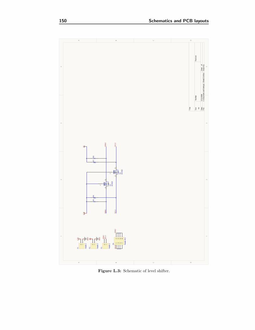
150 Schematics and PCB layouts
11
22
33
44
DD
CC
BB
AA
Titl
e
Num
ber
Rev
isio
nSi
ze A4
Dat
e:17
/12/
2008
Shee
tof
File
:C
:\Doc
umen
tsan
dS
ettin
gs\.
.\Sh
eet2
.Sch
Doc
Dra
wn
By:
D3
G1 S
2
Q1
BSN
20
D3
G1 S
2
Q2
BSN
20
R5
R6
R7
R8
5V3.
3V SDA
1
SCL
1
SDA
2
SCL
2
12
P1 Hea
der2 12
P2 Hea
der2
3.3V 5VGN
D
GN
D
12
P3 Hea
der2
SDA
1SC
L1
SDA
2SC
L2
12
34
56
78
P4 Hea
der4
X2
Figure L.3: Schematic of level shifter.

151
Figure L.4: PCB of level shifter.

152 Schematics and PCB layouts
Figure L.5: PCB board.

Appendix M
Functions used in control loop
The three functions adc convert, receiver convert and controllerdy-namicthrust, that are used when the helicopter is in the state Flight aug-mented, will be explained in this chapter. The functions are shown as flowdiagrams.
adc convertThe function adc convert is shown in figure M.1. An hardware capture andcompare routine runs constantly with 10[ms] intervals. As this is a hard-ware routine its use of the micro controller CPU time is trivial. The routinesets the adc flag each time it has new data to be processed. This flag ischecked when entering the adc convert function. If there are no new dataavailable, it will not do anything and return false. If there is new adc dataready to be processed, the adc convert function will convert the raw datato rad
s and then integrate them. When this has been done, the function willset adc flag to zero and return true.
The whole controller routine period time is thus controlled by the adc flagas long as the controller can execute all its calculations within the 10[ms].

154 Functions used in control loop
Figure M.1: The flow diagram for the adc convert function.

155
receiver convertThe signals coming from the receiver are PWM signals. The receiver convertfunction, which is shown in figure M.2, has to measure these and convertthem into the respective values that are used in the control loop. First thefunction checks that all the receiver channels are working. If they are work-ing it will proceed. Otherwise it will return false.
After checking that all channels are working, the function starts convert-ing them. The values from the receiver are from 0 to 1. The function willfirst calibrate the values so that their midpoint is set to 0.5. Thereafter itwill check if the values are out of the range 0 − 1. If they are lower theywill be set to zero, if they are higher they are set to one. Thereafter it willconvert them with respect to their usage. The pitch, roll and yaw valuesare converted so that their range is from −0.5 to 0.5. All the other valueskeep their range 0 − 1. As the conversion depends on which value is beingconverted, this is coded as a switch-case structure.
controllerdynamicthrustWhen controllerdynamicthrust, see figure M.3, is called, both adc dataand receiver data are available. The controller has to calculate the con-trol signal for each of the four rotors first. This is done by looping fourtimes where the angular velocity contributions to the control signal is firstcalculated. Thereafter the angle contributions to the control signal are cal-culated. These are then multiplied by their respective gains and are finallyadded together for the total control signal to the respective rotor. This canalso been seen in figure 7.4 in chapter 7.
When the control signals for all the rotors has been calculated they aremultiplied with Gain. Thereafter they are subtracted from the Receiverthrust. The resulting servo signals are sent to the motor controllers.

156 Functions used in control loop
Figure M.2: The flow diagram for the receiver convert function.

157
Figure M.3: The flow diagram for the controllerdynamicthrust function.

158 Functions used in control loop


Department of Electrical EngineeringAutomation (AU)Technical University of DenmarkElektrovej building 326DK-2800 Kgs. LyngbyDenmark
www.elektro.dtu.dk/forskning/auTel: (+45) 45 25 35 50Fax: (+45) 45 88 12 95E-mail: [email protected]