The Effect of High-Frequency Trading on Stock Volatility and Price Discovery

X. Frank Zhang Yale University

School of Management (203) 432-7938

frank.zhang@yale.edu

November 2010

I received many helpful comments from Nicholas Barberis, Bill Beaver, Martijn Cremers, Terry Hendershott, Jonathan Ingersoll Jr., Charles Lee, Alina Lerman, Kalin Kolev, Matthew Spiegel, Eric So, Steve Stubben (Stanford discussant), Shyam Sunder, Siew Hong Teoh, Jake Thomas, Rodrigo Verdi, and seminar participants at Goldman Sachs, Stanford University (Summer Camp), University of California at Irvine, and the Wharton school at University of Pennsylvania. I also thank Mark Roemer and Jason Russell at Allianz Global Investors Capital and Ingrid Tierens at Goldman Sachs for detailed discussions on trading and other institutional features. I thank the Yale School of Management for financial support.

The Effect of High-Frequency Trading on Stock Volatility and Price Discovery

Abstract

High-frequency trading has become a dominant force in the U.S. capital market, accounting for

over 70% of dollar trading volume. This study examines the effect of high-frequency trading on

stock price volatility and price discovery. I find that high-frequency trading is positively

correlated with stock price volatility after controlling for firm fundamental volatility and other

exogenous determinants of volatility. The positive correlation is stronger among the top 3,000

stocks in market capitalization and among stocks with high institutional holdings. The positive

correlation is also stronger during periods of high market uncertainty. Furthermore, I find that,

high-frequency trading hinders the market’s ability to incorporate information about firm

fundamentals into asset prices, as high-frequency trading causes stock prices to overreact to

fundamental news. Overall, this paper demonstrates that high-frequency trading generates some

harmful effects for the U.S. capital market.

Keywords: High-frequency trading, trading volume, volatility, return, price discovery.

JEL: G10, G11, G12, G14, G23, M40, M41

1

1. Introduction

This paper examines the impact of high-frequency trading (HFT) on the U.S. capital

market. HFT refers to fully automated trading strategies with very high trading volume and

extremely short holding periods ranging from milliseconds to minutes and possibly hours.

Specifically, this study addresses two broad questions: (1) Does HFT decrease or increase stock

price volatility? and (2) Does HFT aid or hinder the market’s incorporation of news about firm

fundamentals into stock prices?

The motivation for this study is twofold. First, HFT has become a dominant driver of

trading volume in the U.S. capital market. By most accounts, HFT is responsible for more than

half of all equity trades in the United States every day.1 Given its prominence, the SEC and

CFTC have become increasingly concerned about the impact of HFT on capital markets, and are

assessing whether changes are needed in the way HFT is regulated. However, little academic

research has yet examined the effect of HFT on the U.S. capital market. This paper adds to the

accounting and finance literature by documenting a number of consequences of HFT.

A second impetus for this study is the fact that HFT strategies are agnostic to a stock’s

price level and have no intrinsic interest in the fate of companies, leaving little room for a firm’s

fundamentals to play a direct role in its trading strategies. A key objective of the financial

reporting system is to provide a firm’s fundamental information to the capital markets (e.g., the

mission of FASB; Verrecchia 2001). When investors trade stocks on the basis of information

about firm fundamentals, in equilibrium stock prices converge to their fundamental values (e.g.,

Ball and Brown 1968; Kothari 2001; Lee 2001). However, when most trades are based on

statistical and often short-lived correlations in stock returns and investors do not hold stocks for

1 The TABB Group, a consulting company in New York City, estimated that, as of 2009, HFT firms account for 73% of all U.S. equity trading volume. www.tabbgroup.com/PublicationDetail.aspx?PublicationID=505&MenuID=13&ParentMenuID=2&PageID=8..

2

the investment purpose (HFT traders typically do not carry any position overnight), the presence

of efficient pricing becomes more questionable. Theoretical models (Froot, Scharfstein, and

Stein 1992) show that a market with more short-horizon traders performs less efficiently than

one with long-term investors, possibly because short-horizon traders may choose to study

information unrelated to fundamentals. This paper tests such implications and presents an

empirical investigation of the role of HFT in the capital market’s incorporation of fundamental

information into asset prices.

The analysis presented in this paper focuses on a large sample of firms from the CRSP

and the Thomson Reuters Institutional Holdings databases during 1985–2009. I find that

institutional turnover was remarkably stable (around 20% per quarter) throughout the 1985–2009

sample period, even though institutional holdings steadily increased from 40% in 1985 to over

60% in 2009. During the first 10 years of the sample period, stock turnover was also very

stable—around 17% per quarter, a number close to the average institutional turnover over the

same time period. However, stock turnover increased dramatically after 1995, climbing to over

100% by 2009. The drastic divergence between the turnover of stocks and the turnover of

institutional holdings coincides with the emergence and rising popularity of HFT. I estimate that

high-frequency trading was responsible for about 78% of the dollar trading volume in 2009, up

from near zero in 1995. This surge naturally raises concerns regarding the beneficial or harmful

effects of HFT for U.S. capital markets.

My investigation reveals that HFT increases stock price volatility. Specifically, stock

price volatility is positively correlated with HFT after controlling for the volatility of a firm’s

fundamentals and other exogenous volatility drivers. I also explore three institutional features of

HFT and examine the cross-sectional and time-series patterns in the volatility–HFT relationship.

3

First, the positive correlation between volatility and HFT is stronger for the top 3,000 stocks in

market capitalization—a group whose membership parallels that of the Russell 3000 and is often

termed “the investable universe” on Wall Street. Second, the positive correlation is stronger for

stocks with high institutional holdings, a result consistent with the view that high-frequency

traders often take advantage of large trades by institutional investors. Finally, the positive

correlation between HFT and volatility is stronger when market uncertainty is high, a time when

markets are especially vulnerable to aggressive HFT strategies and to the withdrawal of HFT

market-making activities.

I also find that HFT hinders the market’s ability to incorporate news about a firm’s

fundamentals into asset prices, a result consistent with the prediction of Froot, Scharfstein, and

Stein (1992). Using analyst forecast revisions and earnings surprises as proxies for news about

firm fundamentals, this study finds that stock prices react more strongly to news about

fundamentals when HFT is at a high volume, However, the incremental price reactions due to

HFT are almost entirely reversed in the subsequent period. Taken together, the evidence suggests

that HFT exaggerates otherwise-sound price reaction. The price swings introduced by HFT also

represent direct evidence that HFT increases stock price volatility.

This paper contributes to the accounting and finance literature in several important ways.

First, this investigation is the first academic study to examine the role of HFT in the capital

markets. It provides an empirical method to estimate HFT volume for a large dataset and opens

the area for future research. Second, my estimate suggests that HFT accounts for 78% of the total

trading volume of 2009, a number surprisingly close to the estimate of the TABB Group. From

the point of view of market efficiency and social welfare, 78% is clearly excessive if HFT is

meant to provide liquidity. If HFT were to provide all of the market’s liquidity, the volume of

4

HFT would still be at most 50%, although the 50% threshold is surely overstated as it assumes

that all investors trade exclusively with HFT firms, leaving no room for specialists at exchanges

or trade among institutional and individual investors. Third, the evidence that HFT hinders the

market’s incorporation of fundamental news has implications for the financial reporting system

and for regulators. This evidence may help regulators determine how to properly regulate HFT to

allow capital markets to function more efficiently. Finally, this study shows that stock turnover

increased dramatically over the past 15 years owing to the emergence and popularity of HFT.

Such intertemporal structural changes in stock trading volume and price dynamics have broad

implications for studies that assume volatility, trading volume, or price discovery to be stationary

over time (no structural changes are allowed in the classic Fama-MacBeth approach).

The rest of the paper is structured as follows. Section 2 discusses the institutional

background of HFT and reviews the prior literature. Section 3 describes the sample data and

introduces the empirical approach used to estimate the effects of HFT. Section 4 presents the

main results, Section 5 conducts robustness checks, and Section 6 concludes.

2. Background, prior literature, and hypotheses

2.1 High-frequency trading

High-frequency trading firms deploy fully automated trading strategies across one or

more asset classes which identify and profit from short-term (e.g., intra-day) price regularities.

HFT strategies try to earn small amounts of money on each trade—often just a few basis points,

and the small profits from individual trades are amplified by high trading volume. High-

frequency trading can be roughly classified into two types: market making activities and more

aggressive HFT trading strategies (e.g., statistical arbitrage). HFT is a subset of algorithmic

trading, or the use of computer programs for entering trading orders, with the computer

5

algorithm deciding such aspects of the order as the timing, price, and order quantity. However,

HFT distinguishes itself from general algorithmic trading in terms of holding periods and trading

purposes.

Both traditional institutions and HFT firms widely employ algorithmic trading.2 However,

traditional institutions typically hold a stock for the purpose of long-term investment, whereas

HFT firms hold a stock for a only very short period and for the purpose of trading. As shown

below, the recent explosion in trading volume in the U.S. stock market is driven not by

traditional institutions’ algorithmic trading but by a few hundred HFT firms.

During the late 1980s and 1990s, traders abandoned the traditional open-outcry system in

favor of electronic trading desks across the world, as deregulation of the financial markets

prompted a huge shift to screen-based trading. Since the1990s, increased market liquidity and

technological advances have created the ideal conditions for the spread of HFT. The TABB

Group estimates that, as of 2009, between 10 and 20 broker–dealer proprietary trading desks and

fewer than 20 active hedge funds employed HFT techniques. The independent proprietary

trading firms are believed to number between 100 and 300. The several hundred HFT companies

(out of roughly 20,000 firms currently trading in the U.S. markets) are responsible for more than

70% of the trading volume in the U.S. stock market.

A debate has emerged in the business media regarding the benefits and detriments of

HFT, with tensions developing between hedge funds and traditional institutional investors.

Proponents of HFT, who are often hedge fund managers and professionals who provide services

to high-frequency traders, argue that HFT adds liquidity to the market and reduces transaction

costs and spreads for other investors. They also argue that HFT acts as a market maker and aids

2 Pension funds, mutual funds, and other buy-side institutional traders widely use algorithmic trading to divide large orders into small ones to manage market impact and risk.

6

in price discovery. Opponents of HFT, who are often buy-side institutional investors and

professionals who provide services for institutional investors, argue that HFT hurts the ability of

traditional institutional investors to execute orders with limited market impact. Opponents argue

that in their pursuit of market share in trading volume, exchanges and broker-dealers cater to

high-frequency traders at the expense of traditional institutions.

2.2 Prior literature

Several strands of literature touch on related topics, but I am not aware of any academic

research directly examining the role of HFT in the capital markets. The absence of any academic

research on HFT is surprising given its large share of trading volume in the capital markets.

A related literature examines algorithmic/automated trading. This stream of research

generally finds that, as a technology advance over human trading, algorithmic trading is good for

the market. For example, algorithmic trading is weakly negatively correlated with volatility in

the foreign exchange market (Chaboud et al. 2009). On the Deutsche Boerse, algorithmic trading

contributes more than human trading to the discovery of the efficient price (Hendershott and

Riordan 2009). Additionally, algorithmic trading increases liquidity (Hendershott et al. 2010).

Directly comparing this paper with the literature on algorithmic trading is difficult, because both

traditional institutional investors and high-frequency traders widely use algorithmic trading.

Algorithmic trading speeds up order execution and thus represents a technological advance over

human trading. In contrast, HFT has extremely short holding periods, with the purpose of

generating profits. The literature on algorithmic trading examines its benefits and costs relative

to human trading in a market microstructure framework, whereas this paper focuses more on the

interaction between traditional institutional investors and high-frequency traders and its

implications for market efficiency. Of particular interest is the effect of HFT on the the market’s

7

incorporation of firm fundamental information into stock price. Aggressive HFT strategies are

often implemented in dark pools, which have limited data available to the researchers and make

market microstructure studies infeasible.

A fairly large stream of research examines stock price volatility. These studies often

assume that stock price volatility is endogenously determined by the volatility of a stock’s

underlying fundamental value (Scheinkman and Xiong 2003). This literature also shows that

stock price volatility is positively correlated with leverage (Christie 1982), firm age (Pastor and

Veronesi 2003), and growth options (Cao et al. 2008). The evidence on institutional holdings is

mixed. For example, Potter (1992) finds a positive correlation between stock price volatility and

institutional holdings on days surrounding earnings announcements, whereas El-Gazzar (1998)

documents a negative correlation using a different sample and a different set of control variables.

2.3 Does HFT reduce stock price volatility?

Stock return volatility is a basic building block for a number of literatures, such as those

relating to market efficiency, asset allocation, and risk management. High stock volatility is

potentially undesirable for both investors and firms (Bushee and Noe 2000). Risk-averse

investors typically require a higher premium to hold high-volatility stocks, and they react slowly

to fundamental information about high-volatility stocks (Zhang 2006). From a firm’s perspective,

high stock price volatility can increase the perceived riskiness of a firm’s stock and thus increase

a firm’s cost of capital (Froot, Perold, and Stein 1992). High stock price volatility can also make

stock-based compensation more costly (Baiman and Verrecchia 1995) and increase the

likelihood of lawsuits (Francis, Philbrick, and Schipper 1994).

Whether HFT increases or reduces stock price volatility is not obvious. On one hand,

HFT, especially its market-making activity, can reduce stock volatility. HFT firms provide

8

liquidity to the market and enable large block traders to place their trades without significantly

affecting stock prices. HFT market-makers do not profit from stock price movement. Rather,

they generate revenues from the bid–ask spread as well as incentive rebates provided by

electronic communication networks (ECNs), a class of SEC-permitted alternative trading

systems.3

On the other hand, the interaction between HFT and fundamental investors may increase

stock price volatility for at least three reasons. First, as illustrated in the flash crash on May 6th,

2010, high trading volume generated by HFT is not necessarily a reliable indicator of market

liquidity, especially in times of significant volatility. The automated execution of large orders by

fundamental investors, which typically use trading volume as the proxy for liquidity, could

trigger excessive price movement, especially if the automated program does not take prices into

account. Second, HFT is often based on short-term statistical correlations among stock returns. A

large number of unidirectional trades can create price momentum and attract other momentum

traders to the stock, a practice that amplifies price swings and thus increases price volatility.

Positive feedback investment strategies may result in excess volatility even in the presence of

rational speculators (De Long, Shleifer, Summers, and Waldmann 1990).

Finally, high-frequency traders detect and front-run large orders by institutional investors,

a practice that pushes the stock price up (down) if institutional investors have large buy (sell)

orders, thereby increasing stock price volatility.4 One popular, yet controversial, issue related to

front-running is co-locating. HFT firms co-locate their computers physically close to the 3 In a credit structure, ECNs make a profit from paying a credit to liquidity providers, such as high-frequency traders, while charging a debit to liquidity removers. Credits range from $0.002 to $0.00295 per share for liquidity providers, and debits from $0.0025 to $0.003 per share for liquidity removers. The fee can be determined by monthly volume provided and removed or by a fixed structure, depending on the ECN. 4 For example, suppose an institutional investor wants to buy 10,000 shares of JP Morgan and, without HFT firms, the market supplies 10,000 shares at $40.15. An HFT firm steps in and buys these 10,000 shares from the market at $40.15 and then sells them to the institutional investor at $40.18. A similar argument applies to a sell order by an institutional investor.

9

exchanges’ computers to gain millisecond speed advantages, so they can beat slower orders from

buy-side institutional investors to the quote.5 In some cases, HFT firms even co-locate their

computers in the same room as an exchange’s computers. Another controversial HFT strategy is

liquidity detection, which has produced a clash between HFT and traditional investors

resembling the drama of cold-war espionage. To avoid revealing large trades to the open market,

institutional investors often rely on dark pools of liquidity (e.g., Instinet), which are crossing

networks that provide liquidity not displayed on order books. The broker displays only a small

part of the order and leaves a large undisplayed quantity below the surface (a so-called iceberg

order). High-frequency traders employ pattern-recognition software to detect large institutional

orders sitting in dark pools or other liquidity venues. They do so by sending small orders on

reconnaissance missions, in which the small orders interact with large orders by being filled very

quickly. When these interactions happen repeatedly or when orders are executed in amounts

larger than the displayed size, the hidden large order is detected. To counter this HFT effect,

institutions use anti-pattern-recognition software to make customer orders harder to see.

2.4 Does HFT improve price discovery?

Although high frequency trading is short-term in nature, a more interesting question is

whether HFT has an accumulated longer-term effect (e.g., quarterly) when interacted with

fundamental trading. I employ a quarterly window research design for three reasons. First, tick-

by-tick research could potentially produce biased results because many HFT strategies, such as

liquidity detection and other aggressive HFTs, are implemented in dark pools, where transaction

5 Hyde Park Global Investments, a small trading firm based in Atlanta, Georgia, relocated its computer servers to New York to be close to the exchanges and, as a result, shortened the trade time by 21 milliseconds (Source: the April issue of Wired magazine, 2010).

10

data are recorded on the national tape with limited information and with a delay.6 A tick-by-tick

study using open market data is likely to be influenced by HFT’s market-making activities,

which tend to be more beneficial to the capital market than aggressive HFT strategies. Second,

longer-term effects are more interesting and more important from the perspective of market

efficiency. Not only is the impact of HFT on price dynamics often incomplete in the short term

when interacted with fundamental trading, but the research question becomes less interesting if

HFT only delays or accelerates price discovery by milliseconds or seconds. Theoretical models,

such as Froot, Scharfstein, and Stein (1992), have specific predictions on the effect of short-term

traders on market efficiency. Finally, the HFT measure in this study is estimated quarterly, which

restricts my analyses to the quarterly level.

Whether HFT acts to improve price discovery is also not obvious. On one hand, HFT

brings liquidity to the market, as evidenced in increasing trading volume and narrower bid–ask

spreads. The increased liquidity may allow traditional institutional investors to more easily adjust

their portfolios to reflect their fundamentals-based views on company performance. Thus, HFT

may lower the transactions costs faced by institutional investors and help move stock price

towards its fundamental value. On the other hand, HFT is based solely on the statistical

properties of short-term stock returns and is agnostic to the price level—high-frequency traders

can trade 400 million Citibank shares at a price of $3 or $5. High frequency traders typically do

hold the position over a very short period of time and have no intrinsic interest in the fate of

companies. Given that HFT accounts for the lion’s share of trading volume, the interaction

between HFT and fundamental trading could plausibly have some accumulated effect on price

6 Dark pools are recorded to the national consolidated tape, but appear as over-the-counter transactions. Therefore, detailed information about the volumes and types of transactions is often eliminated. Transaction data are typically recorded with a delay. One firm contacted for this study prints dark pool transactions on the tape with a 90-second delay, so the tape does not tell when and where these trades were done.

11

dynamics over longer term. Froot, Scharfstein, and Stein (1992) show theoretically that short

horizon traders may put too much weight on short-term information and not enough on firm

fundamentals, a practice making the market less efficient. A large order by fundamental investor,

coupled with illusive market liquidity as proxied by HFT’s high trading volume, could also

create price momentum or reversal, which could in turn induce other investors, such as

momentum traders, to step in. Such successive effects could potentially cause a stock price to

deviate from its fundamental value in the longer term. Theoretical models in De Long et al.

(1990) and Barberis and Shleifer (2003) suggest that when groups of investors follow simple

positive feedback strategies, stock prices are pushed away from their fundamental values. High-

frequency traders, whose trading strategies are based on short-term statistical correlations, are

classic short-horizon traders and thus are likely to have an impact on market efficiency. This

study examines whether HFT as a whole helps or hinders price discovery at the quarterly level.

3. Sample selection and descriptive statistics

3.1 Sample selection

My initial sample contains all stocks covered by the CRSP and Thomson Reuters

Institutional Holdings databases between the first quarter of 1985 and the second quarter of 2009.

I then delete stocks with a price below $1. As the Thomson Reuters Institutional Holding

database contains only data at the quarterly level, the sample is composed of firm-quarter

observations. Quarterly stock turnover, which is defined as trading volume divided by

outstanding shares, is calculated from CRSP. To account for the double-counting of dealer trades

for Nasdaq firms (Gould and Kleidon 1994), Nasdaq trading volume is divided by two. As will

be clarified later, I use the 1985–1994 period as the estimation period, and use the 1995–2009

period as the main testing sample, which contains 391,013 firm-quarter observations. The sample

12

size varies in some tests to meet other data requirements, such as non-missing analyst forecast

revisions or earnings surprises in the price discovery tests.

I use the Thomson Reuters Institutional Holdings database to calculate institutional

holdings and institutional turnover for each stock each quarter. In the U.S., investment

companies, which include banks, insurance companies, parent companies of mutual funds,

pension funds, university endowments, and numerous other types of professional investment

advisors, are required to file the 13f form with the SEC every calendar quarter, which is covered

by the Thomson Reuters Institutional Holdings database. However, the Thomson Reuters

database does not cover all institutional holdings, since fund managers with less than $100

million assets under their control are not required to file the 13f form, even though they may still

choose to do so. Also, fund managers may omit small holdings (fewer than 10,000 shares or

$200,000) and confidentiality-related holdings from the 13f. Following the literature (Bushee

1998), I define institutions covered by the Thomson Reuters Institutional Holdings database as

“institutional investors” and calculate institutional holdings for a given company by aggregating

stock holdings across all institutional investors and then scaling by the company’s outstanding

shares. Institutional turnover is defined as the aggregate net change in the holdings of a

company’s shares across all institutional investors divided by the average of beginning and

ending institutional holdings.

In general, institutional holdings and net changes are well specified in the Thomson

Reuters database. If a fund manager consistently reports its holdings on each stock, stock

holdings from the previous quarter plus net change in the current quarter should be equal to stock

holdings at the end of the current quarter. One issue with the data is that net changes are coded

incorrectly from the second quarter of 2006 (2006Q2) to the first quarter of 2007 (2007Q1). A

13

manual check of the data revealed that virtually all net changes appear to be coded incorrectly as

stock holdings at the end of the previous quarter multiplied by minus one (-1).7 In light of this

data error, I recalculate net changes as the difference in institutional holdings between two

adjacent quarters for the period between 2006Q2 and 2007Q1. If every institution reports its

holdings each quarter, then the alternative approach to calculate net changes is equivalent to the

main approach. To the extent that the institutional investor universe changes from quarter to

quarter in the Thomson Reuters database, this alternative methodology for the calculation of net

changes is inferior.

Figure 1 plots value-weighted institutional ownership, institutional turnover, and stock

turnover from 1985Q1 to 2009Q2. Institutional ownership steadily increases from 40% in 1985

to over 60% in 2009. Institutional turnover is remarkably stable and stays around 20% each

quarter throughout the sample period. In contrast, stock turnover hovers around 17% between

1985 and 1994 and then increases to 115% in 2008. The gradual increase in stock turnover

beginning in the mid-1990s coincides with the emergence and rising popularity of HFT. For

example, Citadel Investment Group started with bond trades in 1990 and later expanded to the

equity side. Now, Citadel accounts for about 8% of daily trading activity on the NYSE and

Nasdaq.8 In another example, Renaissance Technologies’ Nova Fund became increasingly active

in the mid-1990s, and on a single day in 1997, Nova executions accounted for 14% of the share

volume of the Nasdaq.9

3.2 Measuring high-frequency trading

7 In response to an inquiry about this issue, the Wharton Research Data Service stated that “we provide Thomson data as it is supplied from the vendor, and our policy is to maintain the data integrity so we do not make corrections or any changes to original feed that we receive from the vendor. Unfortunately, Thomson has no plans to fix this problem.” 8 See http://biz.yahoo.com/ic/105/105911.html 9 http://en.wikipedia.org/wiki/Renaissance_Technologies

14

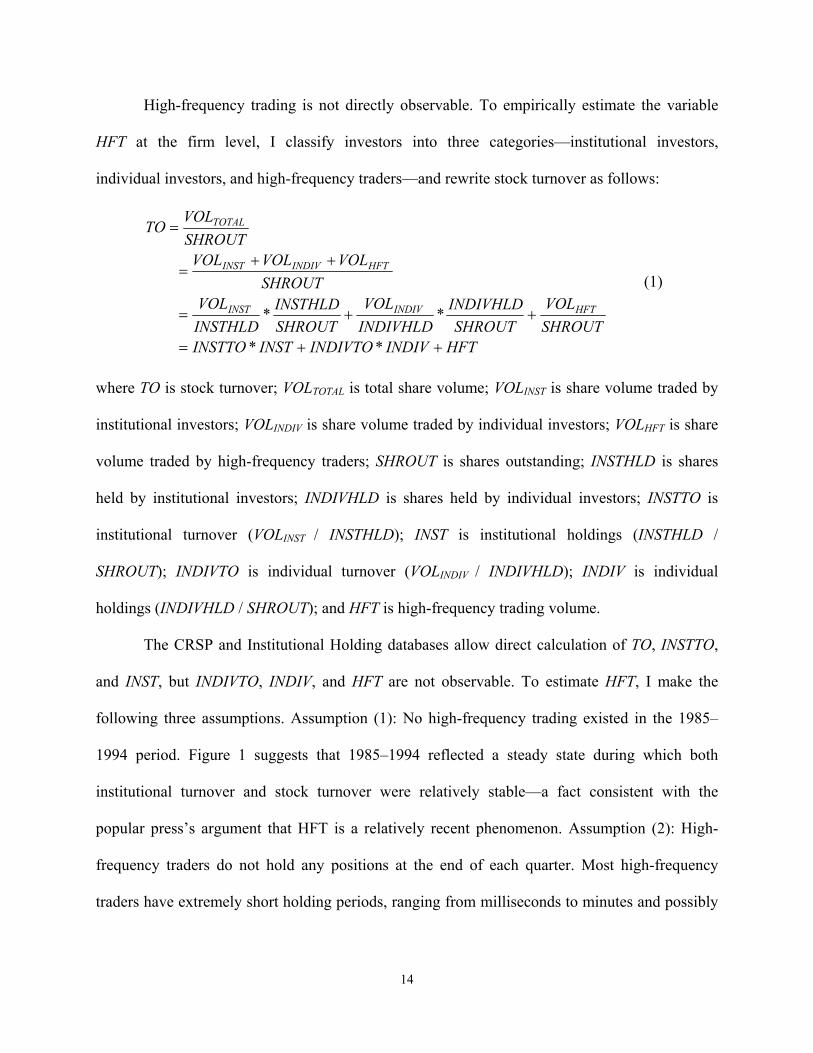
High-frequency trading is not directly observable. To empirically estimate the variable

HFT at the firm level, I classify investors into three categories—institutional investors,

individual investors, and high-frequency traders—and rewrite stock turnover as follows:

HFTINDIVINDIVTOINSTINSTTOSHROUTVOL

SHROUTINDIVHLD

INDIVHLDVOL

SHROUTINSTHLD

INSTHLDVOL

SHROUTVOLVOLVOL

SHROUTVOL

TO

HFTINDIVINST

HFTINDIVINST

TOTAL

++=

++=

++=

=

**

**

(1)

where TO is stock turnover; VOLTOTAL is total share volume; VOLINST is share volume traded by

institutional investors; VOLINDIV is share volume traded by individual investors; VOLHFT is share

volume traded by high-frequency traders; SHROUT is shares outstanding; INSTHLD is shares

held by institutional investors; INDIVHLD is shares held by individual investors; INSTTO is

institutional turnover (VOLINST / INSTHLD); INST is institutional holdings (INSTHLD /

SHROUT); INDIVTO is individual turnover (VOLINDIV / INDIVHLD); INDIV is individual

holdings (INDIVHLD / SHROUT); and HFT is high-frequency trading volume.

The CRSP and Institutional Holding databases allow direct calculation of TO, INSTTO,

and INST, but INDIVTO, INDIV, and HFT are not observable. To estimate HFT, I make the

following three assumptions. Assumption (1): No high-frequency trading existed in the 1985–

1994 period. Figure 1 suggests that 1985–1994 reflected a steady state during which both

institutional turnover and stock turnover were relatively stable—a fact consistent with the

popular press’s argument that HFT is a relatively recent phenomenon. Assumption (2): High-

frequency traders do not hold any positions at the end of each quarter. Most high-frequency

traders have extremely short holding periods, ranging from milliseconds to minutes and possibly

15

hours. Typically, they do not carry any position overnight. 10 Assumption (3): Individual

investors’ trading behavior relative to the behavior of institutional investors is on average stable

over time. This assumption does not require individual investors’ trading behavior to be stable

over time. Rather, the assumption states that, if individual investors trade more during some time

period, such as the financial crisis, institutional investors should also trade more during the same

time period.

As this paper is the first to estimate HFT from a common database for a large sample of

data, these three assumptions are meant to be conservative and as simple as possible. A violation

of the first two assumptions is likely to underestimate the magnitude of HFT in the main

sample. 11 Regarding the third assumption, the relationship between individual turnover and

institutional turnover likely varies with firm characteristics and across industries. A more refined

application of assumption (3) would require a regression model of individual turnover on firm

and industry characteristics. I do not follow this path here to avoid the possibility of data mining.

To the extent that a refined model would reduce measurement error in the estimation of the

volume of HFT, the results from a refined model would likely to be stronger than those reported

in this paper.

Assumption (1) enables calculation of INDIVTO and INDIV for the 1985–1994 period,

given that (1) INST + INDIV = 1 and (2) INST*INSTTO + INDIV*INDIVTO = TO. Assumption

(2) suggests that INDIV + INST = 1 for the 1995–2009 period. Assumption (3) allows me to

quantify individual turnover and estimate it for the 1995–2009 period, which is the main test

10 Some HFT strategies, such as statistical arbitrages, carry positions overnight. 11 A violation of the first assumption would suggest overestimation of individual turnover in both the estimation period and the main sample period. A violation of the second assumption would imply overestimation of individual holdings in the main sample.

16

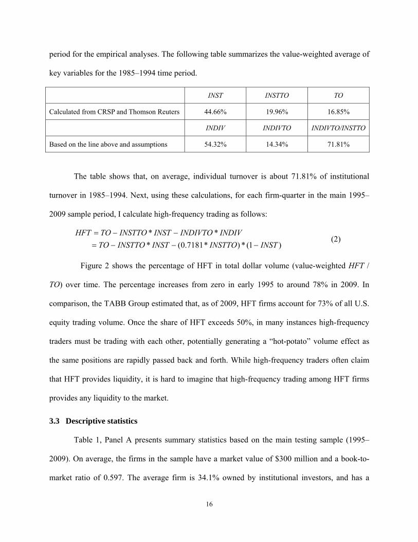
period for the empirical analyses. The following table summarizes the value-weighted average of

key variables for the 1985–1994 time period.

INST INSTTO TO

Calculated from CRSP and Thomson Reuters 44.66% 19.96% 16.85%

INDIV INDIVTO INDIVTO/INSTTO

Based on the line above and assumptions 54.32% 14.34% 71.81%

The table shows that, on average, individual turnover is about 71.81% of institutional

turnover in 1985–1994. Next, using these calculations, for each firm-quarter in the main 1995–

2009 sample period, I calculate high-frequency trading as follows:

)1(*)*7181.0(***

INSTINSTTOINSTINSTTOTOINDIVINDIVTOINSTINSTTOTOHFT

−−−=−−=

(2)

Figure 2 shows the percentage of HFT in total dollar volume (value-weighted HFT /

TO) over time. The percentage increases from zero in early 1995 to around 78% in 2009. In

comparison, the TABB Group estimated that, as of 2009, HFT firms account for 73% of all U.S.

equity trading volume. Once the share of HFT exceeds 50%, in many instances high-frequency

traders must be trading with each other, potentially generating a “hot-potato” volume effect as

the same positions are rapidly passed back and forth. While high-frequency traders often claim

that HFT provides liquidity, it is hard to imagine that high-frequency trading among HFT firms

provides any liquidity to the market.

3.3 Descriptive statistics

Table 1, Panel A presents summary statistics based on the main testing sample (1995–

2009). On average, the firms in the sample have a market value of $300 million and a book-to-

market ratio of 0.597. The average firm is 34.1% owned by institutional investors, and has a

17

stock volatility of 3.3%. High-frequency traders, on average, trade 3.1% of outstanding shares

each quarter. Panel B of Table 1 shows the correlation matrix. HFT is positively related to stock

volatility (VOLT), with a Pearson correlation of 0.078 and a Spearman correlation of 0.090,

supporting the hypothesis that HFT increases volatility in univariate analysis. HFT is highly

positively correlated with firm size (SIZE), confirming the anecdotal evidence that high-

frequency traders focus on large-capitalization stocks. Stock volatility is strongly positively

correlated with fundamental volatility (Pearson correlation = 0.412 with DISP) and negatively

correlated with firm size (Pearson correlation = -0.351).

Panel C of Table 1 shows the Spearman correlation between contemporaneous stock

returns and trading activities. When stock returns are positive, they are positively correlated with

trading activities, with correlations of 0.227, 0.221, and 0.053 with TO, INSTTO, and HFT,

respectively. When stock returns are negative, they are negatively correlated with trading

activities, with correlations of -0.174, -0.158, and -0.077 with TO, INSTTO, and HFT,

respectively. These correlations suggest that trading activities are not directional and tend to be

more active for both extremely high and extremely low returns.12

4. Research design and results

4.1 Research design

Two major issues affected the design of empirical tests. First, as shown in Figure 2, HFT

is not stationary but increases from near zero in 1995 to about 78% in 2009, suggesting the

presence of structural changes in trading behavior between 1995 and 2009. Second, HFT is

measured with error, and such measurement error may affect my statistical tests. 12 The prior literature finds that trading volume is positively correlated with past returns (e.g., Lee and Swaminathan 2000) and negatively correlated with future returns (e.g., Datar, Naik, and Radcliffe 1998). One key innovation of this paper is to examine the effect of trading activities on stock returns based on the nature of news (positive vs. negative earnings news).

18

To address these two issues, I use a difference-in-difference-in-difference approach.

Specifically, in Sections 4.2 and 4.3, I first employ a fixed-effect model with both firm and time

(year-quarter) fixed effects. The model of firm- and time-fixed effects is essentially equivalent to

the difference-in-differences approach common in the literature. For example, to examine the

impact of HFT on stock volatility in Section 4.2, the fixed-effect model compares changes in

stock volatility experienced by high-HFT stocks with changes experienced by low-HFT stocks.

The firm fixed effect controls for differences across firms, and the time fixed effect controls for

differences over time, forcing the regression to estimate a difference in differences. This fixed-

effect approach is widely used to test the impact of structural changes, such as the impact of

algorithmic trading on liquidity (Hendershott et al. 2010). To address potential correlation among

regression residuals, I allow for residuals to be clustered by firm.

Next, in Section 4.4, I use the difference between the results from the main sample period

(1995–2009) and the results from the estimation period (1985–1994) to identify the impact of

HFT. By assuming the absence of HFT during 1985–1994, I assume that measurements from the

estimation period reflect only systematic measurement error of HFT. As long as systematic

measurement error is time-invariant, the difference between the results from the 1985–1994 time

period and the results from the 1995–2009 time period should reflect only the incremental effect

of HFT on stock volatility and price discovery. I specifically consider the possibility of time-

varying measurement error in Section 5.

4.2 Does HFT affect stock volatility?

To examine the effect of HFT on stock volatility, I control for the determinants of stock

volatility as suggested in prior literature. Many studies suggest that stock volatility is determined

yet not fully explained by a firm’s fundamental volatility (Shiller 1981; Scheinkman and Xiong

19

2003; Paster and Veronesi 2003; Wei and Zhang 2006). Three variables capture fundamental

volatility: earnings surprise volatility (sd∆ROE), sales growth volatility (sdSGR), and analyst

forecast dispersion (DISP). Prior studies show that stock volatility is associated with firm age

and institutional holdings (Paster and Veronesi 2003; El-Gazzar 1998), so I include firm age

(AGE) and institutional holdings (INST) as control variables. Prior literature also suggests that

leverage and market microstructure affect stock volatility (Christie 1982; Cheung and Ng 1992).

Accordingly, I include market leverage (LEV) and the inverse of stock price (1/P) in the model.

Finally, since stock volatility may be related to risk, I include three common return factors (SIZE,

BM, and RET_12) as additional controls. Specifically, I employ the following regression

model:13

teeffectsfixedTimeeffectsfixedFIRMRETBMSIZEPINSTAGELEVDISPsdSGRROEsdHFTVOLT

++++++++++++Δ++=

____12_)/1( 11109876

543210

ββββββββββββ

(3)

where VOLT is volatility, HFT is high-frequency trading, sd∆ROE is earnings surprise volatility,

sdSGR is sales growth volatility, DISP is analyst forecast dispersion, LEV is market leverage,

AGE is firm age, INST is institutional holdings, SIZE is firm size, BM is the book-to-market ratio,

RET_12 is the past 12-month stock returns, and 1/P is the inverse of stock price. The appendix

provides detailed definitions of the variables.

Panel A of Table 2 presents the results of tests on the relation between HFT and stock

price volatility. The dependent variables are stock price volatility based on daily returns (VOLT)

in the first column and stock volatility based on daily highs and lows (HLVOLT) in the second

column. Both columns reveal that HFT exhibits a strong positive correlation with stock price

volatility after controlling for other drivers of volatility. For example, the coefficient on HFT is 13 The fixed-effects approach also controls for variations in information flow across firms and across time, which may be correlated with stock volatility (Ross 1989).

20

1.084 (t = 59.62) in the first column. Given the mean VOLT of 0.033 and the standard deviation

of HFT of 0.341, a one standard deviation increase in HFT increases stock volatility by about

11.2%.

The coefficients on the control variables are in line with prior literature. First, stock price

volatility is positively correlated with proxies for fundamental volatility (earnings surprise

volatility, sales growth volatility, and analyst forecast dispersion). Second, stock price volatility

is negatively associated with firm age and institutional holdings, consistent with the findings of

Paster and Veronesi (2003) and of El-Gazzar (1998). Third, stock price volatility exhibits a

positive correlation with market leverage, suggesting that stocks with higher leverage tend to be

more volatile. Market micro-structure also affects stock volatility, with low-price stocks

associated with higher volatility. Lastly, volatility is positively related to firm size and price

momentum and negatively related to the book-to-market ratio, suggesting that large glamour

stocks with strong past performance tend to be more volatile.

The positive correlation between HFT and volatility is consistent with the view that HFT

increases volatility, but it does not establish causality. Next, I consider some exogenous shocks

to HFT by exploring the NYSE automated quote dissemination in 2003 (Henderschott et al.

2010). The NYSE started to autoquote the first stock on January 29, 2003 and autoquote the last

block of stocks on May 27, 2003. Accordingly, I examine changes in stock volatility and HFT

from the last quarter before autoquote (2002Q4) to the first quarter after autoquote (2003Q3). To

the extent that autoquote facilitates HFT for NYSE stocks, I expect that increases in HFT are

more likely to capture true high-frequency trading for NYSE stocks than for other stocks.

Therefore, I expect a positive coefficient on D*∆HFT in the following model.

21

teRETBMSIZEPINSTLEVDISP

sdSGRROEsdHFTDHFTDVOLT

+Δ+Δ+Δ+Δ+Δ+Δ+Δ+

Δ+ΔΔ+Δ+Δ++=Δ

12_)/1(

*

12

11109876

543210

βββββββ

ββββββ (4)

Where D equals 1 for NYSE stocks and 0 otherwise. All other variables are the change

version of the variables in equation (3), where changes are measured from 2002Q4 to 2003Q3.

Compared to equation (3), I drop firm age because changes in firm age are constant across firms.

In regression (4), I essentially use other exchange stocks as the benchmark and test the

incremental effect of the NYSE autoquote on stock volatility. Panel B of Table 2 shows that the

coefficients on D*∆HFT are significantly positive, consistent with my expectation.

To further substantiate the HFT volatility argument, I explore some institutional features

of HFT by examining cross-sectional and time-series variations in the relationship between stock

price volatility and HFT. First, I consider whether a stock is among the top 3,000 stocks based on

the market value of equity at the end of May. The top 3,000 stocks roughly correspond to the

Russell 3000 Index, which the capital management industry widely perceives to constitute the

investable universe. For a given firm, in a given year the market value of equity in May is

assigned to the next 12-month period, because Russell rebalances its index in early June.

Theoretically, nothing stops hedge funds from trading small stocks. Nevertheless, every

investment firm contacted for this study restricts itself to an “investable universe,” which is often

limited to the Russell 3000. The profit opportunity of tiny stocks is often considered to be too

small to be of interest to large hedge funds. Therefore, the HFT measure should better capture

high-frequency trading and thus exhibit a stronger correlation with stock price volatility for the

top 3,000 stocks.

Second, I explore the role of time-series variations in HFT. By and large, high-frequency

traders fall into two categories: market makers and more aggressive HFT strategies. While more

22

aggressive HFT strategies tend to add to stock price volatility, market-making activities may

reduce stock volatility. Unlike specialists at exchanges, who are constrained by regulatory

requirements to stay active at all times and provide bids upon request, high-frequency traders are

free to engage in or desist from market-making activities as they see fit. High-frequency traders

prefer a stable price for their market-making activities, as they do not profit from price

movement. They can cease market-making activity if the market conditions are not right for

them to make profits—a scenario more likely under conditions of high market uncertainty.14 On

the other hand, big swings in stock prices could create stronger intra-day correlations in stock

returns and order imbalance, promoting a larger volume of aggressive HFT. Altogether, HFT

should make stocks more volatile when market uncertainty is high (when the VIX index is above

its historic median).

Third, I examine the role of institutional holdings in HFT. As discussed earlier,

practitioners often argue that high-frequency traders take advantage of institutional traders to

benefit themselves. One popular approach among high-frequency traders is to front-run large

trades by institutional investors, a practice that pushes stock prices too high (low) when

institutional investors want to buy (sell). As a result, such HFT behavior naturally increases stock

price volatility. Therefore, the positive correlation between HFT and stock price volatility is

expected to be greater for stocks with high institutional holdings (INST above the median).

Table 3 reports empirical results on these three empirical predictions. The main variables

of interest are the interaction terms between HFT and a dummy variable introduced for each

14 One example of disappearing liquidity is the flash crash on May 6, 2010, when the Dow lost nearly 1,000 points (about 9.2%) in a matter of minutes. During that time, liquidity evaporated from the market, sending shares of some big-name companies (e.g., Accenture) momentarily to a penny when they could not find a bid. To make things worse, the non-transparency that stems from high-frequency trades (which can happen in milliseconds) makes tracking the trades virtually impossible. It took SEC, which has unlimited access to data, more than five months to determine what caused the flash crash.

23

empirical test (regression). Consistent with my predictions, I find that the interaction term is

positive and significant across all three columns in Table 3.

Overall, the evidence strongly supports the first hypothesis—that HFT increases stock

volatility. The positive correlation between HFT and stock price volatility is stronger for stocks

in the investable universe, stronger for stocks with high institutional holdings, and stronger

during periods of high market uncertainty.

4.3 Does HFT improve price discovery?

This section addresses the role of HFT in the market’s incorporation of news about

company fundamentals into stock prices. As discussed earlier, the empirical tests in this

investigation are conducted at the quarterly level. Given that the quarterly level is unlikely to be

the ideal setting for testing the price discovery hypothesis, the results in this test serve as a lower

bound for the possible impact of HFT. If I observe significant results at the quarterly level, it

would be relatively safe to conclude that HFT affects price discovery. However, if I do not

observe significant results, then HFT may still have an effect.

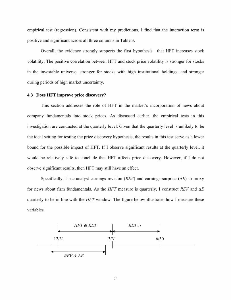
Specifically, I use analyst earnings revision (REV) and earnings surprise (∆E) to proxy

for news about firm fundamentals. As the HFT measure is quarterly, I construct REV and ∆E

quarterly to be in line with the HFT window. The figure below illustrates how I measure these

variables.

12/31 3/31 6/30

HFT & RETt RETt+1

REV & ∆E

24

REV is the consensus analyst earnings forecast in the last month of each calendar quarter

minus the consensus forecast three months prior, scaled by stock price in the last month of the

calendar quarter. As I/B/E/S reports its monthly files on the third Thursday of each month, the

REV window may lead the HFT window by 5–10 business days, leaving the market enough time

to react to the revision news. ∆E and HFT align in such a way that the earnings announcement

date falls in the HFT window. I require the earnings announcement date to be no more than three

months after the fiscal quarter ending date.

For each type of fundamental news, I employ two regression models. Taking REV as an

example,

tt

ttttt

eeffectsfixedTimeeffectsfixedFirmRETBMSIZEHFTREVHFTRET

+++++++++=

−

−−

____12_*)(

16

15143210

ααααααα

(5)

tt

ttttt

eeffectsfixedTimeeffectsfixedFirmRETBMSIZEHFTREVHFTRET

+++++++++=

−

−−+

____12_*)(

16

151432101

βββββββ

(6)

In Equation (5) the dependent variable is contemporaneous stock returns, and in Equation

(6) the dependent variable is future stock returns. The earnings-return literature suggests that

HFT21 αα + should be positive in Equation (5). A positive coefficient on REV ( HFT21 ββ + ) in

Equation (6) indicates a post-news drift, whereas a negative coefficient indicates a reversal. Of

interest is the sign of 2β relative to the signs of 2α and 1β .

Table 4 reports the results of estimations (5) and (6) with respect to analyst forecast

revisions. The first three models are based on contemporaneous stock returns. The first column

shows that contemporaneous returns and revisions are strongly positively correlated, a result

consistent with the general finding in the accounting literature that stock prices react positively to

earnings news. The second column shows an 2α̂ equal to 0.472 (t = 4.53), suggesting that the

25

market reaction to earnings revisions is stronger for high-HFT stocks. This basic result is

unchanged if the earnings–return relation are allowed to vary with SIZE, BM, and RET_12 (as in

column (3) ). The last three models, columns (4)–(6), are based on future stock returns. Column

(4) shows a negative coefficient on REV, indicating that stock prices reverse in the subsequent

three months. This evidence of price reversal differs from the price drift evidence documented in

the prior literature in two respects. First, the price drift based on cross-sectional analysis is much

weaker in more recent years, as compared to the early sample in Stickel (1991). Second, the

price drift is stronger for small firms, some of which are excluded from this study’s sample

owing to missing institutional data. When, in Section 5.2, I expand the sample to all firms and to

earlier years, I observe a price drift in both the 1977–1984 and 1985–1994 time periods. Column

(5) reveals that 2̂β is negative ( 2β̂ = -0.417) and significant (t = -3.41), suggesting that stock

prices reverse more for high-HFT stocks. This result still holds when the earnings–return relation

is allowed to vary with SIZE, BM, and RET_12 (as in column (6) ).

Table 5 reports the results of estimations (5) and (6) when I use earnings surprises to

proxy for fundamental news. The results are qualitatively similar to those reported in Table 4,

with positive coefficients on ∆E*HFT in regressions using contemporaneous returns and negative

coefficients on ∆E*HFT in regressions using future returns.

Taken together, these results suggest that HFT hinders price discovery. HFT pushes stock

prices too far in the direction of earnings news and, as a result, stock prices reverse in the

subsequent months after the initial reaction. In fact, 2α̂ and 2̂β are very similar in magnitude but

have opposite signs, suggesting that the incremental HFT-driven market reaction to earnings

news is almost fully reversed in the subsequent months. HFT-related price reaction and

subsequent reversal are at least consistent with two possible mechanisms. First, HFT and

26

traditional investors’ trading are independent. HFT first reacts to earnings news and moves the

stock price. Traditional investors trade stocks subsequently and further move the price, without

adjusting the initial price reaction introduced by HFT. Second, HFT interacts with traditional

investors. It is possible that HFT front-runs large orders of institutional investors, who tend to

trade in the direction of earnings news, a practice driving up (down) the price after good (bad)

news. It is also possible that HFT induces more momentum traders to trade in the direction of

earnings news and thus may create a short-term overreaction.15 Data limitations preclude me

from identifying the exact underlying mechanism (or combination), which I leave for future

research.

4.4 Quantifying the effect of measurement error on the variable HFT

As HFT is not directly observable, some simplifying assumptions apply to empirically

estimating HFT. Consequently, HFT is estimated with error. This section presents an attempt to

gauge the effect of measurement error on the key findings.

As shown in Section 3.2, the INDIVTO/INSTTO ratio estimated in the 1985–1994 period

is used to calculate HFT for each firm-quarter in the 1995–2009 period. Similarly, I can calculate

HFT for each firm-quarter in the 1985–1994 period using Equation (2). Under the assumption

that no HFT exists in the 1985–1994 period, this HFT estimate captures measurement error

introduced in the estimation process.16 By construction, the value-weighted average of HFT

15 Another possibility is that HFT identify mispricing opportunities and trade more as an arbitrageur when traditional investors overreact more to earnings news. I view this mechanism to be less likely for two reasons. First, HFT typically does not trade on fundamental earnings news and is agnostic about the price level. High frequency traders are less likely than traditional investors to identify mispricing opportunities. Second, if HFT works as a mispricing arbitrage force, it should reduce mispricing relative to stocks with less HFT. Also, it is unclear why, with such high trading volume, HFT cannot eliminate mispricing. Nevertheless, I cannot rule out the possibility that HFT trades more when there is more mispricing. 16 Note that this study conservatively assumes no HFT in the 1985–1994 period. To the extent that HFT existed in 1985–1994, the effect of measurement error is likely to be overstated because so-called measurement error actually captures HFT.

27

across all firm-quarters should be zero for 1985–1994.17 I redo the main tests presented in Tables

2, 4, and 5 using the 1985–1994 sample. If measurement error has no impact on my results, the

coefficients on key variables of interest should be close to zero.

In the volatility test (column (1) in Panel A of Table 2), I find the coefficient on HFT to

be positive ( 1̂β = 0.538) and highly significant (t = 27.94), suggesting that measurement error

does affect stock volatility. As HFT is measured relative to the value-weighted

INDIVTO/INSTTO ratio, a positive coefficient on HFT means higher than average stock turnover

is positively related to stock volatility. In essence, measurement error in the HFT variable

captures the positive correlation between trading volume and volatility that is not due to HFT

(e.g., Lee et al. 1994). More importantly, the coefficient estimate of 0.538 is much smaller than

the estimate of 1.084 reported in Table 2. By conservatively assuming that HFT only captures

measurement error in the 1985–1994 period, I view that the difference between these two

coefficient estimates (1.084 – 0.538 = 0.546) represents the incremental effect of HFT on stock

volatility. This incremental coefficient (0.546) is still highly significant (t = 28.21).

Table 6 reports the results of robustness test involving price discovery. Panel A is based

on analyst forecast revisions and Panel B is based on earnings surprises. In both panels, the

coefficients on fundamental news are highly positive in column (1), confirming the earnings–

return relationship for the 1985–1994 period. More importantly, the coefficients on HFT*REV

and HFT*∆E are insignificantly different from zero across all models, suggesting that the

market’s incorporation of fundamental news is uncorrelated with measurement error.

Overall, I conclude that measurement error in HFT accounts for about 50% of the

volatility results but does not affect the price discovery results. Measurement error has a smaller

17 In a regression framework as used in the paper, the mean value of HFT is irrelevant because it is captured by the intercept (firm and time dummies).

28

impact on the price discovery test possibly because of its better research design of using the

interaction terms.

5. Robustness checks

5.1 Does HFT capture the changing nature of individual investors’ trading behavior?

The approach described in Section 4.4 is effective as long as HFT measurement error is

time-invariant. However, for at least three reasons measurement error could change over time.

First, over time individual investors have become more active in stock trading owing to

technological advances such as the availability of online trading. As a result, overall stock

turnover has increased over time and the HFT measure captures this increase in individual

trading behavior.18 Second, over time traditional institutional investors have engaged in more

intra-quarter trades (the purchase and subsequent sale of a stock in a single calendar quarter). Yet

these trades are not captured by the measure of institutional turnover as institutions only file 13f

forms quarterly. Finally, in recent years institutions have tended to use more principal bids.

When using a principal bid, an institution turns over its trading list to a large broker, such as

Goldman Sachs, in lieu of trading the list by itself. Most principal bids are submitted before the

market opens at 9:30am. The broker then nets out buys and sells from different client institutions

and trades the net balance in dark pools or in the open market.

The first reason for the possible presence of time-variant measurement error—more

activity from individual investors—is my main concern and is empirically examined in this

section. The second possible source of measurement error—more intra-quarter trading—is of

less importance because traditional institutions have a fixed annual turnover budget and typically

18 Note that this alternative explanation is inconsistent with anecdotal evidence of the rising popularity and dominance of HFT in the U.S. capital market (as discussed earlier).

29

cannot buy and sell stocks in the same quarter. The typical institution’s budget allows for

approximately 130–150% turnover per year and does not change much over time. In fact,

institutions often have to explain intra-quarter trades to their clients because these trades are

perceived as abnormal when compared to the typical stock holding period of 9–12 months. The

last possible source of measurement error, more principal bids, is not a matter of much concern

because additional principal bids would bias the measurement of HFT downward. Institutions

report principal trades in form 13f, but brokers net out these trades from among different

institutions and only trade the residual net balance in the market. Institutional turnover includes

all principal trades, whereas total stock turnover only captures trading of the net balance. Thus,

in the presence of more principal trades HFT would be understated.

To test for the presence of the first source of time-variant measurement error, the

following model explores cross-sectional and time-series variations in HFT:

tePLEVDISPsdSGRROEsdRETBMSIZEINDIVHFT

+++++Δ+++++=

)/1(12_

9876

543210

ββββββββββ

(7)

The main variable of interest in Equation (7) is INDIV. If individual investors have traded

more frequently in recent years and HFT captures such individual trading behavior, then HFT

should be higher for stocks with higher individual holdings, resulting in a positive coefficient on

INDIV.

Table 7 reports the results of three incrementally richer specifications of Equation (7).

Model (1) is a univariate regression of HFT on INDIV. The coefficient on INST is highly

negative. This finding is not consistent with an increase in individual investors’ trading behavior

relative to that of institutional investors over time. In Model (2), I add three common return

factors. I control for firm size, because size often proxies for liquidity. Model (2) shows that

HFT is positively correlated with firm size, the book-to-market ratio, and price momentum.

30

More importantly, the coefficient on INDIV remains highly negative. In Model (3), I add

additional proxies for fundamental volatility (sd∆ROE, sdSGR, and DISP), market leverage, and

the reciprocal of the stock price. Market leverage and stock price also capture liquidity in the

absence of HFT.19 The coefficient on INDIV remains highly significant, with t-statistics over 20.

HFT is also positively correlated with fundamental volatility and market leverage.

Overall, the results are inconsistent with the view that HFT captures increased individual

trading behavior over time. As institutional holdings and individual holdings sum to one, the

negative correlation between HFT and individual holdings implies a positive correlation between

HFT and institutional holdings—a result consistent with the theory that high-frequency traders

target traditional institutional investors. This evidence is also in line with anecdotal observations

that many HFT strategies, such as liquidity detection, are deliberately implemented to front-run

trades by institutional investors.

5.2 Does HFT simply reflect the trading volume effect?

As institutional holdings and institutional turnover are relatively stable over time, HFT

and stock turnover (TO) are highly correlated in the 1995–2009 sample period, with a Spearman

correlation coefficient of 0.60. Given such a high degree of correlation, one might wonder

whether the HFT measure simply reflects a universal trading volume effect (Lee and

Swaminathan 2000). As the analysis in Section 4.4 shows, HFT does not play any significant

role in price discovery in the base estimation period (1985–1994), a result inconsistent with the

universal trading volume effect. However, the insignificant results in the 1985–1994 sub-period

may be sample-specific. In this section, I expand my sample to include all stocks with non-

19 Traditional liquidity measures, such as trading volume and bid-ask spread, are not included in the model as these measures are affected by HFT.

31

missing values of TO and extend the sample period back to 197720 Then, I partition the sample

period into three sub-periods: 1977–1984, 1985–1994, and 1995–2009. If trading volume has a

consistent effect on price discovery, I expect high-TO stocks to overreact to fundamental news

and to subsequently exhibit a reversal in all three sub-periods, paralleling the HFT results

documented in Tables 4 and 5.

Table 8 reports the empirical results from the analysis on trading volume. The regression

in Panel A uses analyst forecast revisions to proxy for fundamental news, and the regression in

Panel B uses earning surprises to proxy for fundamental news. The main variables of interest are

REV*TO and ∆E*TO. In Panel A, the first block shows regressions of contemporaneous stock

returns. Returns are positively correlated with analyst revisions, and the positive correlation is

stronger for high-TO stocks in all three sub-periods. The second block of Panel A shows

regressions of future stock returns. In Models 1 and 3 the coefficients on REV are significantly

positive, suggesting a price drift after analyst revisions in the 1977–1984 and 1985–1994 sub-

periods. Model 5 reports a negative coefficient on REV, indicating a price reversal in the 1995–

2009 sub-period. More importantly, the coefficient on REV*TO is significantly negative only in

Model 6, suggesting a stronger price reversal for high-TO stocks in the 1995–2009 sub-period

that echoes the HFT results in Table 4. The insignificant coefficients on REV*TO in the 1977–

1984 and the 1985–1994 sub-periods suggest that HFT does not capture a universal trading

volume effect.

The results from the earnings surprises regressions in Panel B are largely similar. The

market shows a stronger response to earnings surprises for high-TO stocks. In all three sub-

periods, stock prices drift in the direction of earnings news after the initial market reaction. In the

20 Analyst forecast revisions were first made available on I/B/E/S in 1977.

32

1977–1984 and 1985–1994 sub-periods, trading volume does not have a significant impact on

post-surprise drift, and in the 1995–2009 sub-period trading volume tends to attenuate the drift..

Taken together, the above results reveal that the impact of trading volume on price

discovery is not uniform throughout the whole sample period (1977–2009). The results offer no

evidence of price reversals and the associated effect on trading volume in the 1977–1984 and the

1985–1994 sub-periods. The results on trading volume in the 1995–2009 sub-period are more

similar to the HFT results documented in Tables 4 and 5. Overall, the evidence is more

consistent with the HFT effect than with the trading-volume effect.

5.3 Different windows to determine the INDIVTO/INSTTO ratio

The main analysis uses the 1985–1994 time period to determine the ratio of institutional

turnover to individual turnover. The choice of 1985–1994 is arbitrary, although Figure 1 suggests

that during this period both stock turnover and institutional turnover were in a steady state. In a

robustness check, I use the 1985–1989 time period as the baseline for key calculations (see

section 3.2), and the tenor of the original findings remains unchanged. For example, the

coefficient on HFT becomes 1.051 (t = 62.19) in column (1) of Table 2. The coefficients on

REV*HFT come to equal 0.466 (t = 4.71) and -0.453 (t = -3.79) in columns (2) and (5) of Table

4, respectively. I also rerun my analysis using 1988–1989 as the baseline time period, as the

1988–1989 time period excludes the crash of 1987. The results produced by this additional

estimation are again qualitatively similar to the original findings.

5.4 The double-count issue for Nasdaq firms

To account for market-maker activity in calculating Nasdaq trading volume, I divide

Nasdaq firms’ trading volume by two in the main analysis. As a robustness check, I treat trading

volume as it is and redo the analysis. The use of this single-count specification does not

33

significantly alter the original findings. For example, the coefficient on HFT is newly estimated

to equal 0.901 (t = 64.43) in column (1) of Table 2. The coefficients on REV*HFT come to equal

0.641 (t = 8.64) and -0.283 (t = -3.27) in columns (2) and (5) of Table 4, respectively. Since

market-maker activity varies across Nasdaq firms and over time, a uniform cutoff may still

introduce measurement error into the trading volume measure. As an alternative approach, I

exclude Nasdaq firms from the sample and find the tenor of the paper unchanged.21 For example,

the coefficient on HFT is re-estimated to equal 0.809 (t = 39.14) in column (1) of Table 2. The

coefficients on REV*HFT come to equal 0.324 (t = 2.55) and -0.493 (t = -3.33) in columns (2)

and (5) of Table 4, respectively.

6. Conclusions and discussion

In this paper, I empirically estimate the volume of HFT in the U.S. capital market and

examine the effect of HFT on stock price volatility and price discovery. Analysis shows that, in

terms of trading volume, HFT has become the dominant force in the equity market, accounting

for about 78% of total dollar trading volume in the first two quarters of 2009 (the most recent

data available). From the liquidity perspective, 78% is clearly excessive. If HFT provides all

liquidity needed in the market, the maximum percentage is 50%, where the maximum is surely

overstated as it assumes everybody trades with HFT firms (with no trade for specialists at

exchanges and no trade among institutional and/or individual investors). HFT has brought total

share turnover to over 100% per quarter in recent years. In contrast, quarterly institutional

turnover has been remarkably stable over time, averaging about 20% over the past 25 years.22

21 Conceptually, it is suboptimal to exclude Nasdaq firms from the sample. Nasdaq was at the forefront of electronic trading. Most high-frequency traders started their HFT strategies from Nasdaq. 22 It should be noted that institutional holdings have gradually increased from 40% in the 1980s to over 60% in recent years.

34

More importantly, this study shows that HFT is positively correlated with stock price

volatility after controlling for the volatility of a stock’s fundamentals and other volatility drivers.

This positive correlation is especially strong for the top 3,000 stocks in market capitalization and

for stocks with high institutional holdings. The positive correlation between HFT and volatility is

also stronger during periods of high market uncertainty. Taken together, the results are consistent

with the view that HFT increases volatility. This study also offers evidence that HFT hinders

price discovery. HFT causes stock prices to overreact to news about company fundamentals

(proxied by analyst forecast revision and earnings surprises). The incremental price changes due

to HFT are almost entirely reversed in the subsequent periods.

This analysis warrants several caveats. First, as HFT is not directly observable,

estimating the volume of HFT requires some simplifying assumptions. To the extent that the

calculation of HFT suffers from measurement error, some estimated regression coefficients could

be biased. I conduct a number of robustness checks to alleviate concerns about measurement

error. Nevertheless, I must acknowledge the presence of measurement error and the concerns that

it may raise. Second, HFT is measured at the quarterly level owing to data limitations. The

quarterly research design has some important advantages: it gives a good overall picture of

HFT’s share of total U.S. trading volume, and it describes the prolonged effect HFT has on price

dynamics and on market efficiency. However, the quarterly research design has some limitations.

Data permitting, it would be interesting to use intra- or inter-day data to study the impact of HFT,

especially on the underlying mechanism of the price discovery results. The last caveat is the

issue of endogeneity in the volatility test. This paper argues that HFT increases volatility.

However, the possibility of reverse causality could be used as a counter-argument since volatile

stocks and volatile markets could attract high-frequency traders. I use the exogenous shock of

35

NYSE autoquote and variations in the HFT-volatility relation to partially address this issue. In

addition, the finding that HFT causes stock prices to over-react to news about fundamentals, and

that this over-reaction is subsequently corrected, represents direct evidence supporting the

hypothesis that HFT creates volatility.

Given that HFT constitutes the lion’s share of trading volume in today’s capital markets,

the paucity of academic research on HFT is surprising. While this study sheds light on the role of

HFT in the capital market and suggests its implications for market efficiency, many questions

remain unanswered. For example, does HFT reduce volatility in certain scenarios, such as during

periods of very low uncertainty? Do HFT’s market-making activities and more aggressive

strategies have different implications for market efficiency? Do high-frequency traders withdraw

liquidity when uncertainty is extremely high, as evidenced in the flash crash on May 6, 2010?

What is the overall benefit of HFT, relative to its costs to the market? Would a small tax on

financial transactions, such as a 0.1% tax on the value of traded stock, make HFT more

beneficial for the market?23 It would also be important to investigate the implication of HFT for

individual investors. Conceivably, sophisticated technologies give high-frequency traders a large

advantage over regular investors, creating a disincentive for individuals of modest means to

invest in the markets. I leave these questions for future research.

23 From a policy perspective, reining in the scope of HFT would be fairly easy if HFT were found to be harmful to the capital market. A small tax on financial transactions would dramatically reduce the volume of high-frequency trading. For example, one top hedge fund contacted for this study claims to use a strategy that makes five basis points per trade with an average transaction cost of three basis points. A tax of 0.05% would undermine this particular hedge fund’s high-frequency trades.

36

References Baiman, S. and R. Verrecchia. 1995. Earnings and price-based compensation contracts in the

presence of discretionary trading and incomplete contracting. Journal of Accounting and Economics 20, 93-121.

Ball, R. and P. Brown. 1968. An empirical evaluation of accounting income numbers. Journal of

Accounting Research 6, 159-178. Barberis, N. and A. Shleifer. 2003. Style investing. Journal of Financial Economics 68, 161-199. Bushee, B. 1998. The influence of institutional investors on myopic R&D investment behavior.

The Accounting Review 73, 19-45. Bushee, B. and C. Noe. 2000. Corporate disclosure practices, institutional investors, and stock

return volatility. Journal of Accounting Research 38, 171-202. Cao, C., T. Simin, and J. Zhao. 2008. Can growth options explain the trend in idiosyncratic risk?

Review of Financial Studies 21, 2599-2633. Chaboud, A., B. Chiquoine, E. Hjalmarsson, and C. Vega. 2009. Rise of the machines:

algorithmic trading in the foreign exchange market. Federal Reserve Board, working paper. Cheung Y. and L. Ng. 1992. Stock price dynamics and firm size: An empirical investigation. The

Journal of Finance 47 (5), 1985-1997. Christie A. 1982. The stochastic behavior of common stock variances: value, leverage and

interest rate effects. Journal of Financial Economics 10, 407-432. Datar, V., N. Naik, and R. Radclifffe. 1998. Liquidity and asset returns: An alternative test.

Journal of Financial Markets 1, 203-220. De Long, B.J., A. Shleifer, L. Summers, and R. Waldmann. 1990. Positive feedback investment

strategies and destabilizing rational speculation. Journal of Finance 45, 379-396. El-Gazzar, S. 1998. Predisclosure information and institutional ownership: A cross-sectional

examination of market revaluations during earnings announcement periods. The Accounting Review 73, 119-130.

Francis, J., D. Philbrick, and K. Schipper. 1994. Shareholder litigation and corporate disclosures.

Journal of Accounting Research 32, 137-164. Froot, K, A. Perold, and J. Stein. 1992. Shareholder trading practices and corporate investment

horizons. Journal of Applied Corporate Finance, 42-58. Froot, K, D. Scharfstein, and J. Stein. 1992. Herd on the street: Informational inefficiencies in a

market with short-term speculation. Journal of Finance 47, 1461-1484.

37

Gould, J. and A. Kleidon. 1994. Market maker activity on Nasdaq: Implications for trading

volume. Stanford Journal of Law, Business, and Finance 1, 1-17. Hendershott, T., C. Jones, and A. Menkveld. 2010. Does algorithmic trading improve liquidity?

Journal of Finance, forthcoming. Hendershott, T. and R. Riordan. 2009. Algorithmic trading and information. UC Berkeley,

working paper. Kothari, S.P., 2001. Capital markets research in accounting. Journal of Accounting and

Economics 31, 105-231. Lee, C. 2001. Market efficiency and accounting research. Journal of Accounting and Economics

31, 233-253. Lee, C., M. Ready, and P. Seguin. 1994. Volume, volatility, and NYSE trading halts. Journal of

Finance 49, 183-214. Lee, C. and B. Swaminathan. 2000. Price momentum and trading volume. Journal of Finance,

2017-2069. Pastor, L. and P. Veronesi. 2003. Stock valuation and learning about profitability. Journal of

Finance 58, 1749–1789. Potter, G. 1992. Accounting earnings announcements, institutional investor concentration, and

common stock returns. Journal of Accounting Research 30, 146-155. Ross, S. 1989. Information and volatility: The no-arbitrage martingale approach to timing and

resolution irrelevancy. The Journal of Finance 25, 1-17. Scheinkman, J. and W. Xiong. 2003. Overconfidence and speculative bubbles. Journal of

Political Economy 111, 1183-1219. Shiller, R. 1981. Do stock prices move too much to be justified by subsequent changes in

dividend? American Economic Review 71, 421-436. Stickel, S. 1991. Common stock returns surrounding earnings forecast revisions: More puzzling

evidence. The Accounting Review 66, 402-416. Verrecchia, R. 2001. Essays on disclosure. Journal of Accounting and Economics 32, 97-180. Wei, S. and C. Zhang. 2006. Why did individual stocks become more volatile? The Journal of

Business 79 (1). Zhang, X. F. 2006. Information uncertainty and stock returns. Journal of Finance 61, 105-137.

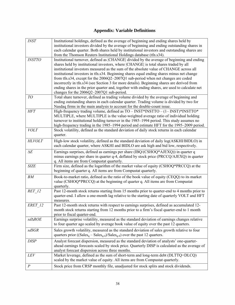
38

Appendix: Variable Definitions

INST Institutional holdings, defined as the average of beginning and ending shares held by institutional investors divided by the average of beginning and ending outstanding shares in each calendar quarter. Both shares held by institutional investors and outstanding shares are from the Thomson Reuters Institutional Holdings database (tfn.s34).

INSTTO Institutional turnover, defined as |CHANGE| divided by the average of beginning and ending shares held by institutional investors, where |CHANGE| is total shares traded by all institutional investors measured as the sum of the absolute value of CHANGE across all institutional investors in tfn.s34. Beginning shares equal ending shares minus net change from tfn.s34, except for the 2006Q2–2007Q1 sub-period when net changes are coded incorrectly in tfn.s34 (see Section 3 for more details). Beginning shares are derived from ending shares in the prior quarter and, together with ending shares, are used to calculate net changes for the 2006Q2–2007Q1 sub-period.

TO Total share turnover, defined as trading volume divided by the average of beginning and ending outstanding shares in each calendar quarter. Trading volume is divided by two for Nasdaq firms in the main analysis to account for the double-count issue.

HFT High-frequency trading volume, defined as TO – INST*INSTTO – (1– INST)*INSTTO* MULTIPLE, where MULTIPLE is the value-weighted average ratio of individual holding turnover to institutional holding turnover in the 1985–1994 period. This study assumes no high-frequency trading in the 1985–1994 period and estimate HFT for the 1995–2009 period.

VOLT Stock volatility, defined as the standard deviation of daily stock returns in each calendar quarter.

HLVOLT High-low stock volatility, defined as the standard deviation of daily log(ASKHI/BIDLO) in each calendar quarter, where ASKHI and BIDLO are ask high and bid low, respectively.

∆E Earnings surprises, defined as earnings per share (IBQ/(CSHOQ*AJEXQ)) in quarter q minus earnings per share in quarter q-4, deflated by stock price (PRCCQ/AJEXQ) in quarter q. All items are from Compustat quarterly.

SIZE Firm size, defined as the logarithm of the market value of equity (CSHOQ*PRCCQ) at the beginning of quarter q. All items are from Compustat quarterly.

BM Book-to-market ratio, defined as the ratio of the book value of equity (CEQQ) to its market value (CSHOQ*PRCCQ) at the beginning of quarter q. All items are from Compustat quarterly.

RET_12 Past 12-month stock returns starting from 15 months prior to quarter-end to 4 months prior to quarter-end. I allow a one-month lag relative to the starting date of quarterly VOLT and HFT measures.

ERET_12 Past 12-month stock returns with respect to earnings surprises, defined as accumulated 12-month stock returns starting from 12 months prior to a firm’s fiscal quarter-end to 1 month prior to fiscal quarter-end.

sd∆ROE Earnings surprise volatility, measured as the standard deviation of earnings changes relative to four quarter ago scaled by average book value of equity over the past 12 quarters.

sdSGR Sales growth volatility, measured as the standard deviation of sales growth relative to four quarters prior ((Salesq – Salesq-4)/Salesq-4) over the past 12 quarters.

DISP Analyst forecast dispersion, measured as the standard deviation of analysts’ one-quarter-ahead earnings forecasts scaled by stock price. Quarterly DISP is calculated as the average of analyst forecast dispersion across three months.

LEV Market leverage, defined as the sum of short-term and long-term debt (DLTTQ+DLCQ) scaled by the market value of equity. All items are from Compustat quarterly.

P Stock price from CRSP monthly file, unadjusted for stock splits and stock dividends.

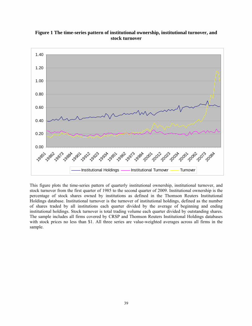
39

Figure 1 The time-series pattern of institutional ownership, institutional turnover, and stock turnover

0.00

0.20

0.40

0.60

0.80

1.00

1.20

1.40

1985

119

862

1987

319

884

1990

119

912

1992

319

934

1995

119

962

1997

319

984

2000

120

012

2002

320

034

2005

120

062

2007

320

084

Institutional Holdings Institutional Turnover Turnover

This figure plots the time-series pattern of quarterly institutional ownership, institutional turnover, and stock turnover from the first quarter of 1985 to the second quarter of 2009. Institutional ownership is the percentage of stock shares owned by institutions as defined in the Thomson Reuters Institutional Holdings database. Institutional turnover is the turnover of institutional holdings, defined as the number of shares traded by all institutions each quarter divided by the average of beginning and ending institutional holdings. Stock turnover is total trading volume each quarter divided by outstanding shares. The sample includes all firms covered by CRSP and Thomson Reuters Institutional Holdings databases with stock prices no less than $1. All three series are value-weighted averages across all firms in the sample.

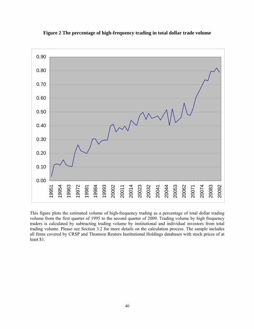
40

Figure 2 The percentage of high-frequency trading in total dollar trade volume

0.00

0.10

0.20

0.30

0.40

0.50

0.60

0.70

0.80

0.9019

951

1995

4

1996

3

1997

2

1998

1

1998

4

1999

3

2000

2

2001

1

2001

4

2002

3

2003

2

2004

1

2004

4

2005

3

2006

2

2007

1

2007

4

2008

3

2009

2

This figure plots the estimated volume of high-frequency trading as a percentage of total dollar trading volume from the first quarter of 1995 to the second quarter of 2009. Trading volume by high frequency traders is calculated by subtracting trading volume by institutional and individual investors from total trading volume. Please see Section 3.2 for more details on the calculation process. The sample includes all firms covered by CRSP and Thomson Reuters Institutional Holdings databases with stock prices of at least $1.

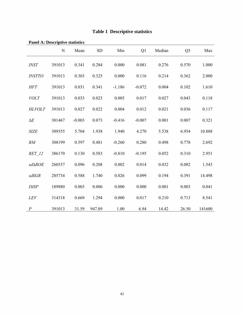
41

Table 1 Descriptive statistics

Panel A: Descriptive statistics

N Mean SD Min Q1 Median Q3 Max

INST 391013 0.341 0.284 0.000 0.081 0.276 0.570 1.000

INSTTO 391013 0.303 0.325 0.000 0.116 0.214 0.362 2.000

HFT 391013 0.031 0.341 -1.186 -0.072 0.004 0.102 1.610

VOLT 391013 0.033 0.023 0.005 0.017 0.027 0.043 0.118

HLVOLT 391013 0.027 0.022 0.004 0.012 0.021 0.036 0.117

∆E 301467 -0.003 0.073 -0.416 -0.007 0.001 0.007 0.321

SIZE 309355 5.704 1.938 1.940 4.270 5.538 6.954 10.888

BM 308199 0.597 0.481 -0.260 0.280 0.498 0.778 2.692

RET_12 386170 0.130 0.583 -0.810 -0.195 0.052 0.310 2.951

sd∆ROE 260537 0.096 0.208 0.002 0.014 0.032 0.082 1.543

sdSGR 285734 0.588 1.740 0.026 0.099 0.194 0.391 14.498

DISP 189880 0.003 0.006 0.000 0.000 0.001 0.003 0.041

LEV 314318 0.669 1.294 0.000 0.017 0.210 0.713 8.541

P 391013 31.59 947.89 1.00 6.94 14.42 26.50 141600

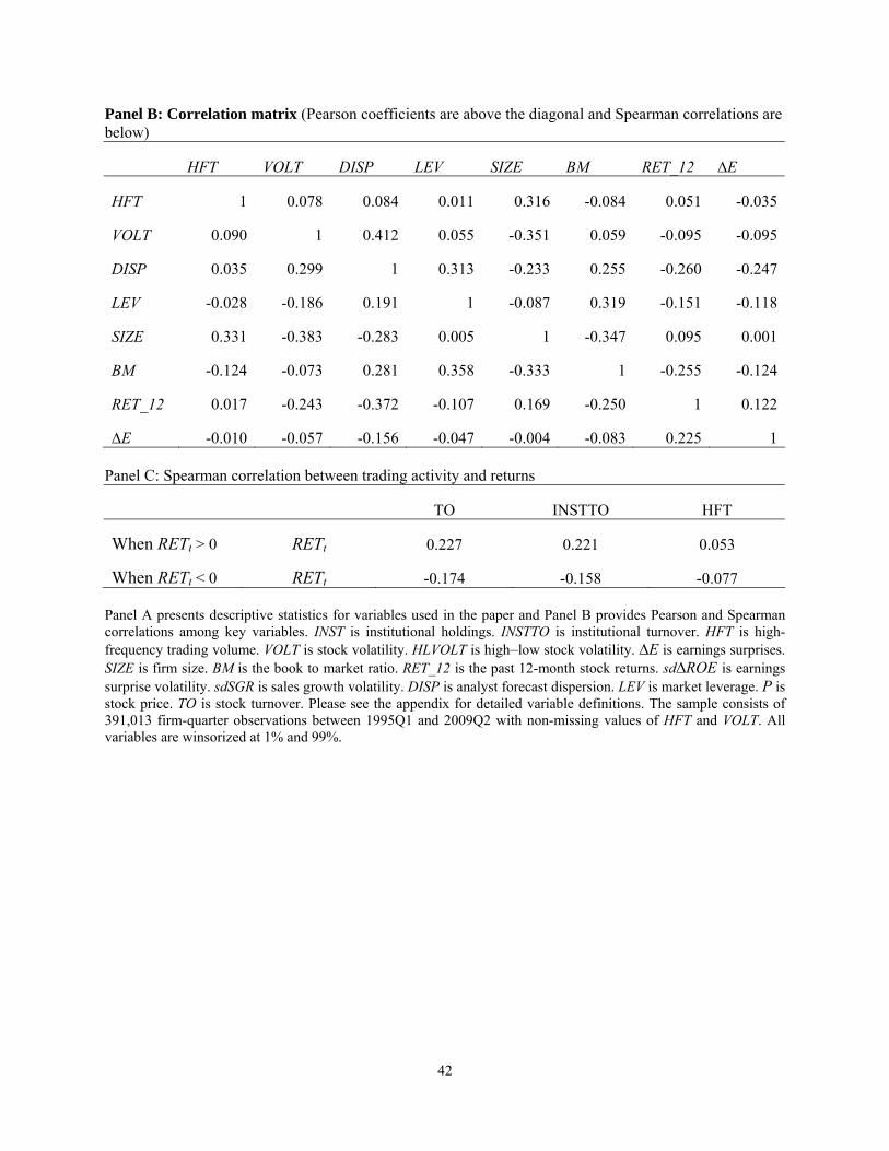
42

Panel B: Correlation matrix (Pearson coefficients are above the diagonal and Spearman correlations are below)

HFT VOLT DISP LEV SIZE BM RET_12 ∆E

HFT 1 0.078 0.084 0.011 0.316 -0.084 0.051 -0.035

VOLT 0.090 1 0.412 0.055 -0.351 0.059 -0.095 -0.095

DISP 0.035 0.299 1 0.313 -0.233 0.255 -0.260 -0.247

LEV -0.028 -0.186 0.191 1 -0.087 0.319 -0.151 -0.118

SIZE 0.331 -0.383 -0.283 0.005 1 -0.347 0.095 0.001

BM -0.124 -0.073 0.281 0.358 -0.333 1 -0.255 -0.124

RET_12 0.017 -0.243 -0.372 -0.107 0.169 -0.250 1 0.122

∆E -0.010 -0.057 -0.156 -0.047 -0.004 -0.083 0.225 1 Panel C: Spearman correlation between trading activity and returns

TO INSTTO HFT

When RETt > 0 RETt 0.227 0.221 0.053

When RETt < 0 RETt -0.174 -0.158 -0.077 Panel A presents descriptive statistics for variables used in the paper and Panel B provides Pearson and Spearman correlations among key variables. INST is institutional holdings. INSTTO is institutional turnover. HFT is high-frequency trading volume. VOLT is stock volatility. HLVOLT is high–low stock volatility. ∆E is earnings surprises. SIZE is firm size. BM is the book to market ratio. RET_12 is the past 12-month stock returns. sd∆ROE is earnings surprise volatility. sdSGR is sales growth volatility. DISP is analyst forecast dispersion. LEV is market leverage. P is stock price. TO is stock turnover. Please see the appendix for detailed variable definitions. The sample consists of 391,013 firm-quarter observations between 1995Q1 and 2009Q2 with non-missing values of HFT and VOLT. All variables are winsorized at 1% and 99%.

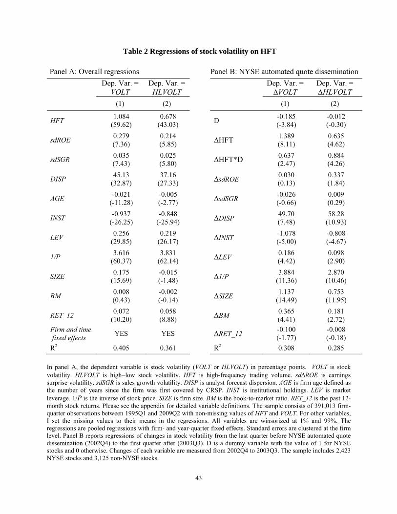
43

Table 2 Regressions of stock volatility on HFT

Panel A: Overall regressions Panel B: NYSE automated quote dissemination

Dep. Var. = VOLT

Dep. Var. = HLVOLT Dep. Var. =

∆VOLT Dep. Var. = ∆HLVOLT

(1) (2) (1) (2)

HFT 1.084 (59.62)

0.678 (43.03) D -0.185

(-3.84) -0.012 (-0.30)

sdROE 0.279 (7.36)

0.214 (5.85) ∆HFT 1.389

(8.11) 0.635 (4.62)

sdSGR 0.035 (7.43)

0.025 (5.80) ∆HFT*D 0.637

(2.47) 0.884 (4.26)

DISP 45.13 (32.87)

37.16 (27.33) ∆sdROE 0.030

(0.13) 0.337 (1.84)

AGE -0.021 (-11.28)

-0.005 (-2.77) ∆sdSGR -0.026

(-0.66) 0.009 (0.29)

INST -0.937 (-26.25)

-0.848 (-25.94) ∆DISP 49.70

(7.48) 58.28

(10.93)

LEV 0.256 (29.85)

0.219 (26.17) ∆INST -1.078

(-5.00) -0.808 (-4.67)

1/P 3.616 (60.37)

3.831 (62.14) ∆LEV 0.186

(4.42) 0.098 (2.90)

SIZE 0.175 (15.69)

-0.015 (-1.48) ∆1/P 3.884

(11.36) 2.870

(10.46)

BM 0.008 (0.43)

-0.002 (-0.14) ∆SIZE 1.137

(14.49) 0.753

(11.95)

RET_12 0.072 (10.20)

0.058 (8.88) ∆BM 0.365

(4.41) 0.181 (2.72)

Firm and time fixed effects YES YES ∆RET_12 -0.100

(-1.77) -0.008 (-0.18)

R2 0.405 0.361 R2 0.308 0.285 In panel A, the dependent variable is stock volatility (VOLT or HLVOLT) in percentage points. VOLT is stock volatility. HLVOLT is high–low stock volatility. HFT is high-frequency trading volume. sd∆ROE is earnings surprise volatility. sdSGR is sales growth volatility. DISP is analyst forecast dispersion. AGE is firm age defined as the number of years since the firm was first covered by CRSP. INST is institutional holdings. LEV is market leverage. 1/P is the inverse of stock price. SIZE is firm size. BM is the book-to-market ratio. RET_12 is the past 12-month stock returns. Please see the appendix for detailed variable definitions. The sample consists of 391,013 firm-quarter observations between 1995Q1 and 2009Q2 with non-missing values of HFT and VOLT. For other variables, I set the missing values to their means in the regressions. All variables are winsorized at 1% and 99%. The regressions are pooled regressions with firm- and year-quarter fixed effects. Standard errors are clustered at the firm level. Panel B reports regressions of changes in stock volatility from the last quarter before NYSE automated quote dissemination (2002Q4) to the first quarter after (2003Q3). D is a dummy variable with the value of 1 for NYSE stocks and 0 otherwise. Changes of each variable are measured from 2002Q4 to 2003Q3. The sample includes 2,423 NYSE stocks and 3,125 non-NYSE stocks.

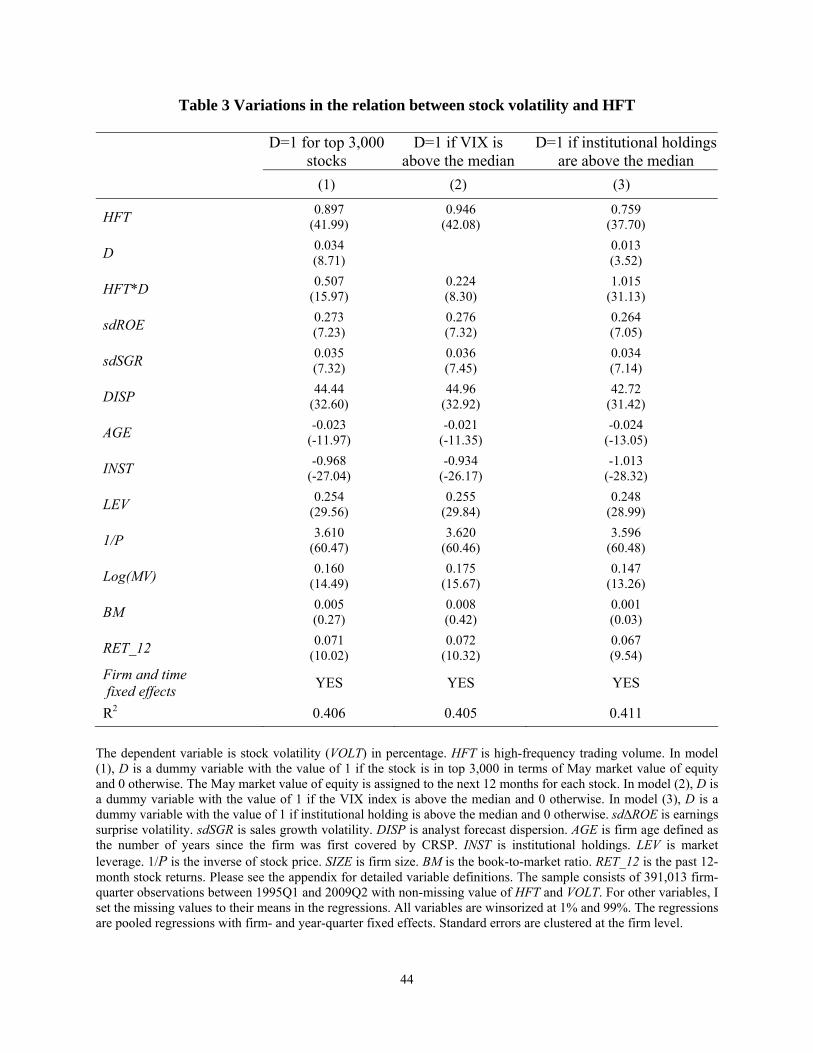
44

Table 3 Variations in the relation between stock volatility and HFT

D=1 for top 3,000 stocks

D=1 if VIX is above the median

D=1 if institutional holdings are above the median

(1) (2) (3)

HFT 0.897 (41.99)

0.946 (42.08)

0.759 (37.70)

D 0.034 (8.71) 0.013

(3.52)

HFT*D 0.507 (15.97)

0.224 (8.30)

1.015 (31.13)

sdROE 0.273 (7.23)

0.276 (7.32)

0.264 (7.05)

sdSGR 0.035 (7.32)

0.036 (7.45)

0.034 (7.14)

DISP 44.44 (32.60)

44.96 (32.92)

42.72 (31.42)

AGE -0.023 (-11.97)

-0.021 (-11.35)

-0.024 (-13.05)

INST -0.968 (-27.04)

-0.934 (-26.17)

-1.013 (-28.32)

LEV 0.254 (29.56)

0.255 (29.84)

0.248 (28.99)

1/P 3.610 (60.47)

3.620 (60.46)

3.596 (60.48)

Log(MV) 0.160 (14.49)

0.175 (15.67)

0.147 (13.26)

BM 0.005 (0.27)

0.008 (0.42)

0.001 (0.03)

RET_12 0.071 (10.02)

0.072 (10.32)

0.067 (9.54)

Firm and time fixed effects YES YES YES

R2 0.406 0.405 0.411 The dependent variable is stock volatility (VOLT) in percentage. HFT is high-frequency trading volume. In model (1), D is a dummy variable with the value of 1 if the stock is in top 3,000 in terms of May market value of equity and 0 otherwise. The May market value of equity is assigned to the next 12 months for each stock. In model (2), D is a dummy variable with the value of 1 if the VIX index is above the median and 0 otherwise. In model (3), D is a dummy variable with the value of 1 if institutional holding is above the median and 0 otherwise. sd∆ROE is earnings surprise volatility. sdSGR is sales growth volatility. DISP is analyst forecast dispersion. AGE is firm age defined as the number of years since the firm was first covered by CRSP. INST is institutional holdings. LEV is market leverage. 1/P is the inverse of stock price. SIZE is firm size. BM is the book-to-market ratio. RET_12 is the past 12-month stock returns. Please see the appendix for detailed variable definitions. The sample consists of 391,013 firm-quarter observations between 1995Q1 and 2009Q2 with non-missing value of HFT and VOLT. For other variables, I set the missing values to their means in the regressions. All variables are winsorized at 1% and 99%. The regressions are pooled regressions with firm- and year-quarter fixed effects. Standard errors are clustered at the firm level.

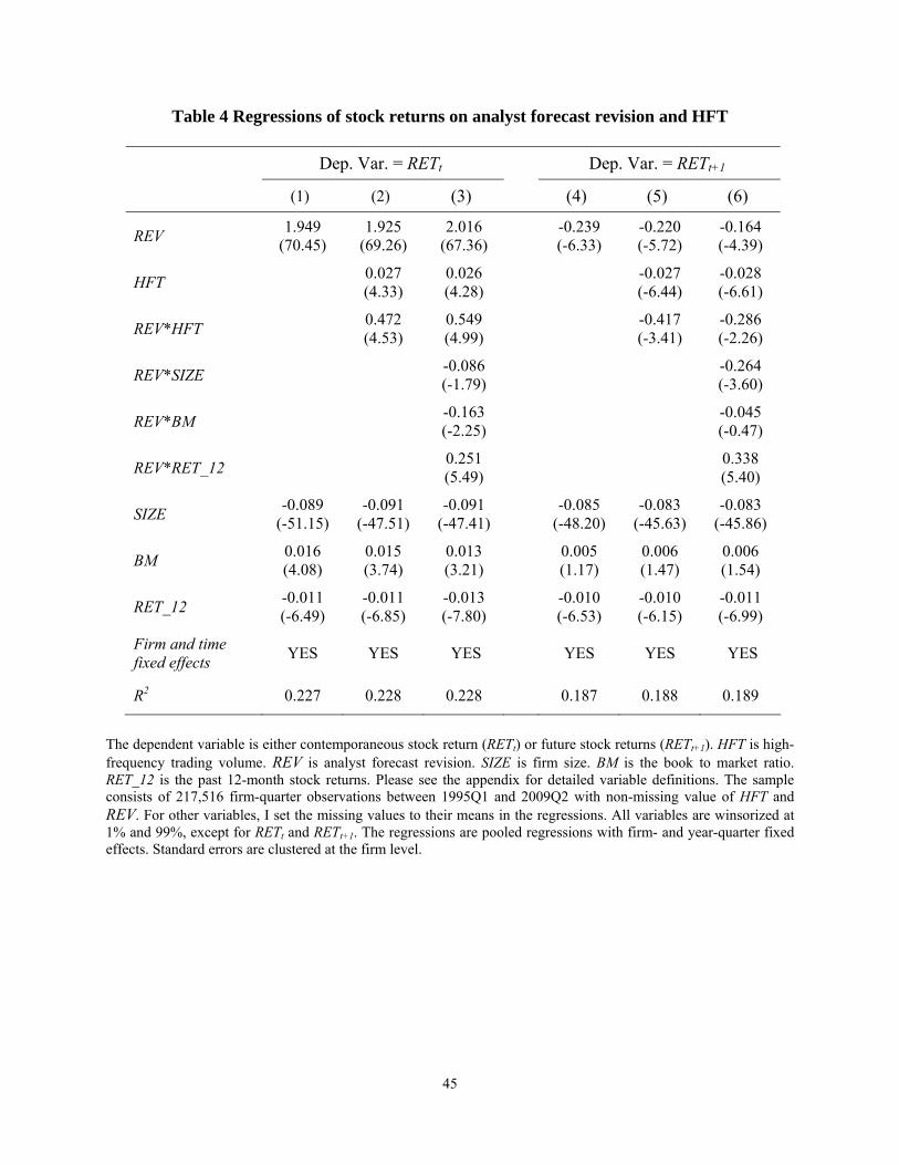
45

Table 4 Regressions of stock returns on analyst forecast revision and HFT

Dep. Var. = RETt Dep. Var. = RETt+1

(1) (2) (3) (4) (5) (6)

REV 1.949 (70.45)

1.925 (69.26)

2.016 (67.36) -0.239

(-6.33) -0.220 (-5.72)

-0.164 (-4.39)

HFT 0.027 (4.33)

0.026 (4.28) -0.027

(-6.44) -0.028 (-6.61)

REV*HFT 0.472 (4.53)

0.549 (4.99) -0.417

(-3.41) -0.286 (-2.26)

REV*SIZE -0.086 (-1.79) -0.264

(-3.60)

REV*BM -0.163 (-2.25) -0.045

(-0.47)

REV*RET_12 0.251 (5.49) 0.338

(5.40)

SIZE -0.089 (-51.15)

-0.091 (-47.51)

-0.091 (-47.41) -0.085

(-48.20) -0.083

(-45.63) -0.083

(-45.86)

BM 0.016 (4.08)

0.015 (3.74)

0.013 (3.21) 0.005

(1.17) 0.006 (1.47)

0.006 (1.54)

RET_12 -0.011 (-6.49)

-0.011 (-6.85)

-0.013 (-7.80) -0.010

(-6.53) -0.010 (-6.15)

-0.011 (-6.99)

Firm and time fixed effects YES YES YES YES YES YES

R2 0.227 0.228 0.228 0.187 0.188 0.189

The dependent variable is either contemporaneous stock return (RETt) or future stock returns (RETt+1). HFT is high-frequency trading volume. REV is analyst forecast revision. SIZE is firm size. BM is the book to market ratio. RET_12 is the past 12-month stock returns. Please see the appendix for detailed variable definitions. The sample consists of 217,516 firm-quarter observations between 1995Q1 and 2009Q2 with non-missing value of HFT and REV. For other variables, I set the missing values to their means in the regressions. All variables are winsorized at 1% and 99%, except for RETt and RETt+1. The regressions are pooled regressions with firm- and year-quarter fixed effects. Standard errors are clustered at the firm level.

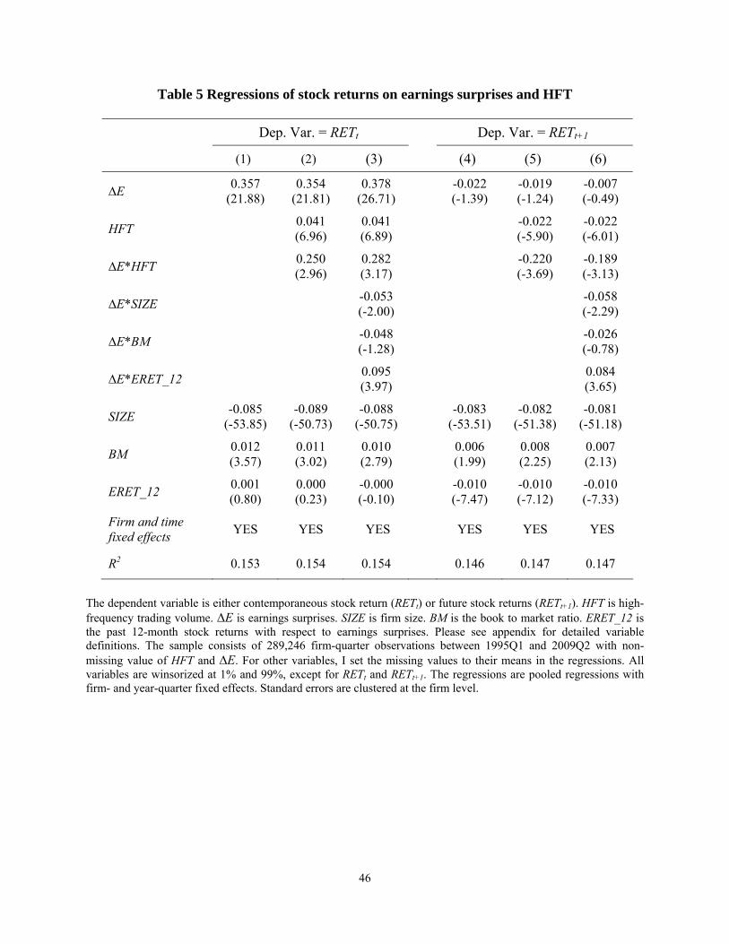
46

Table 5 Regressions of stock returns on earnings surprises and HFT

Dep. Var. = RETt Dep. Var. = RETt+1

(1) (2) (3) (4) (5) (6)

∆E 0.357 (21.88)

0.354 (21.81)

0.378 (26.71) -0.022

(-1.39) -0.019 (-1.24)

-0.007 (-0.49)

HFT 0.041 (6.96)

0.041 (6.89) -0.022

(-5.90) -0.022 (-6.01)

∆E*HFT 0.250 (2.96)

0.282 (3.17) -0.220

(-3.69) -0.189 (-3.13)

∆E*SIZE -0.053 (-2.00) -0.058

(-2.29)

∆E*BM -0.048 (-1.28) -0.026

(-0.78)

∆E*ERET_12 0.095 (3.97) 0.084

(3.65)

SIZE -0.085 (-53.85)

-0.089 (-50.73)

-0.088 (-50.75) -0.083

(-53.51) -0.082

(-51.38) -0.081

(-51.18)

BM 0.012 (3.57)

0.011 (3.02)

0.010 (2.79) 0.006

(1.99) 0.008 (2.25)

0.007 (2.13)

ERET_12 0.001 (0.80)

0.000 (0.23)

-0.000 (-0.10) -0.010

(-7.47) -0.010 (-7.12)

-0.010 (-7.33)

Firm and time fixed effects YES YES YES YES YES YES

R2 0.153 0.154 0.154 0.146 0.147 0.147

The dependent variable is either contemporaneous stock return (RETt) or future stock returns (RETt+1). HFT is high-frequency trading volume. ∆E is earnings surprises. SIZE is firm size. BM is the book to market ratio. ERET_12 is the past 12-month stock returns with respect to earnings surprises. Please see appendix for detailed variable definitions. The sample consists of 289,246 firm-quarter observations between 1995Q1 and 2009Q2 with non-missing value of HFT and ∆E. For other variables, I set the missing values to their means in the regressions. All variables are winsorized at 1% and 99%, except for RETt and RETt+1. The regressions are pooled regressions with firm- and year-quarter fixed effects. Standard errors are clustered at the firm level.

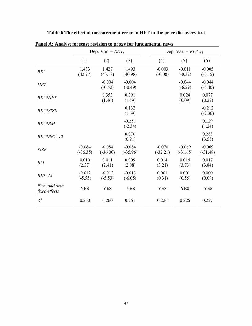
47

Table 6 The effect of measurement error in HFT in the price discovery test

Panel A: Analyst forecast revision to proxy for fundamental news Dep. Var. = RETt Dep. Var. = RETt+1

(1) (2) (3) (4) (5) (6)

REV 1.433 (42.97)

1.427 (43.18)

1.493 (40.98) -0.003

(-0.08) -0.011 (-0.32)

-0.005 (-0.15)

HFT -0.004 (-0.52)

-0.004 (-0.49) -0.044

(-6.29) -0.044 (-6.40)

REV*HFT 0.353 (1.46)

0.391 (1.59) 0.024

(0.09) 0.077 (0.29)

REV*SIZE 0.132 (1.69) -0.212

(-2.36)

REV*BM -0.251 (-2.34) 0.129

(1.24)

REV*RET_12 0.070 (0.91) 0.283

(3.55)

SIZE -0.084 (-36.35)

-0.084 (-36.00)

-0.084 (-35.96) -0.070

(-32.21) -0.069

(-31.65) -0.069

(-31.48)

BM 0.010 (2.37)

0.011 (2.41)

0.009 (2.08) 0.014

(3.21) 0.016 (3.73)

0.017 (3.84)

RET_12 -0.012 (-5.55)

-0.012 (-5.53)

-0.013 (-6.05) 0.001

(0.31) 0.001 (0.55)

0.000 (0.09)

Firm and time fixed effects YES YES YES YES YES YES

R2 0.260 0.260 0.261 0.226 0.226 0.227

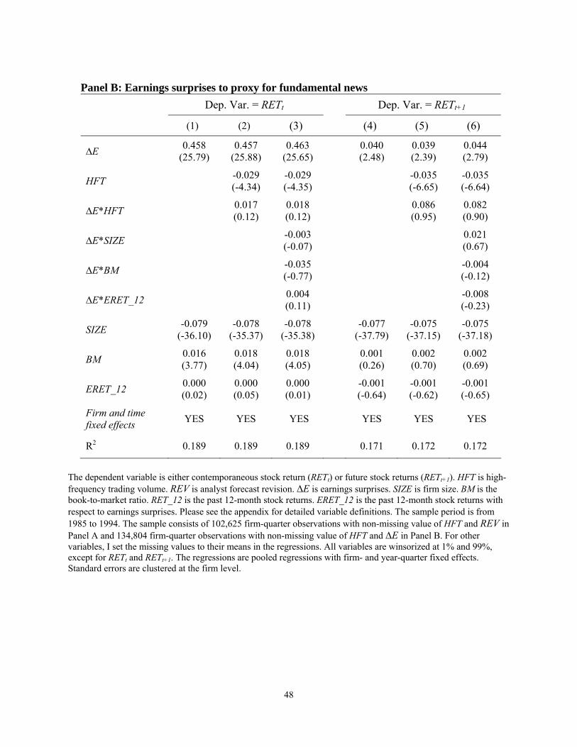
48

Panel B: Earnings surprises to proxy for fundamental news Dep. Var. = RETt Dep. Var. = RETt+1

(1) (2) (3) (4) (5) (6)

∆E 0.458 (25.79)

0.457 (25.88)

0.463 (25.65) 0.040

(2.48) 0.039 (2.39)

0.044 (2.79)

HFT -0.029 (-4.34)

-0.029 (-4.35) -0.035

(-6.65) -0.035 (-6.64)

∆E*HFT 0.017 (0.12)

0.018 (0.12) 0.086

(0.95) 0.082 (0.90)

∆E*SIZE -0.003 (-0.07) 0.021

(0.67)

∆E*BM -0.035 (-0.77) -0.004

(-0.12)

∆E*ERET_12 0.004 (0.11) -0.008

(-0.23)

SIZE -0.079 (-36.10)

-0.078 (-35.37)

-0.078 (-35.38) -0.077

(-37.79) -0.075

(-37.15) -0.075

(-37.18)

BM 0.016 (3.77)

0.018 (4.04)

0.018 (4.05) 0.001

(0.26) 0.002 (0.70)

0.002 (0.69)

ERET_12 0.000 (0.02)

0.000 (0.05)

0.000 (0.01) -0.001

(-0.64) -0.001 (-0.62)

-0.001 (-0.65)

Firm and time fixed effects YES YES YES YES YES YES

R2 0.189 0.189 0.189 0.171 0.172 0.172

The dependent variable is either contemporaneous stock return (RETt) or future stock returns (RETt+1). HFT is high-frequency trading volume. REV is analyst forecast revision. ∆E is earnings surprises. SIZE is firm size. BM is the book-to-market ratio. RET_12 is the past 12-month stock returns. ERET_12 is the past 12-month stock returns with respect to earnings surprises. Please see the appendix for detailed variable definitions. The sample period is from 1985 to 1994. The sample consists of 102,625 firm-quarter observations with non-missing value of HFT and REV in Panel A and 134,804 firm-quarter observations with non-missing value of HFT and ∆E in Panel B. For other variables, I set the missing values to their means in the regressions. All variables are winsorized at 1% and 99%, except for RETt and RETt+1. The regressions are pooled regressions with firm- and year-quarter fixed effects. Standard errors are clustered at the firm level.

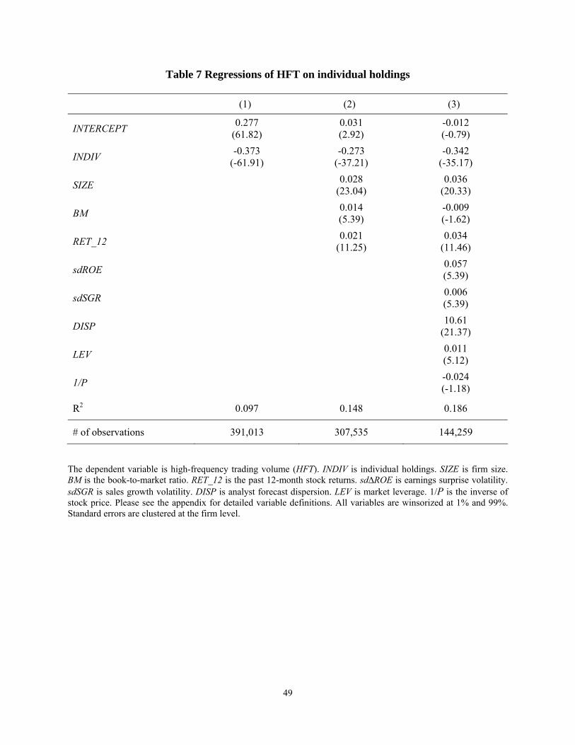
49

Table 7 Regressions of HFT on individual holdings

(1) (2) (3)

INTERCEPT 0.277 (61.82)

0.031 (2.92)

-0.012 (-0.79)

INDIV -0.373 (-61.91)

-0.273 (-37.21)

-0.342 (-35.17)

SIZE 0.028 (23.04)

0.036 (20.33)

BM 0.014 (5.39)

-0.009 (-1.62)

RET_12 0.021 (11.25)

0.034 (11.46)

sdROE 0.057 (5.39)

sdSGR 0.006 (5.39)

DISP 10.61 (21.37)

LEV 0.011 (5.12)

1/P -0.024 (-1.18)

R2 0.097 0.148 0.186

# of observations 391,013 307,535 144,259

The dependent variable is high-frequency trading volume (HFT). INDIV is individual holdings. SIZE is firm size. BM is the book-to-market ratio. RET_12 is the past 12-month stock returns. sd∆ROE is earnings surprise volatility. sdSGR is sales growth volatility. DISP is analyst forecast dispersion. LEV is market leverage. 1/P is the inverse of stock price. Please see the appendix for detailed variable definitions. All variables are winsorized at 1% and 99%. Standard errors are clustered at the firm level.

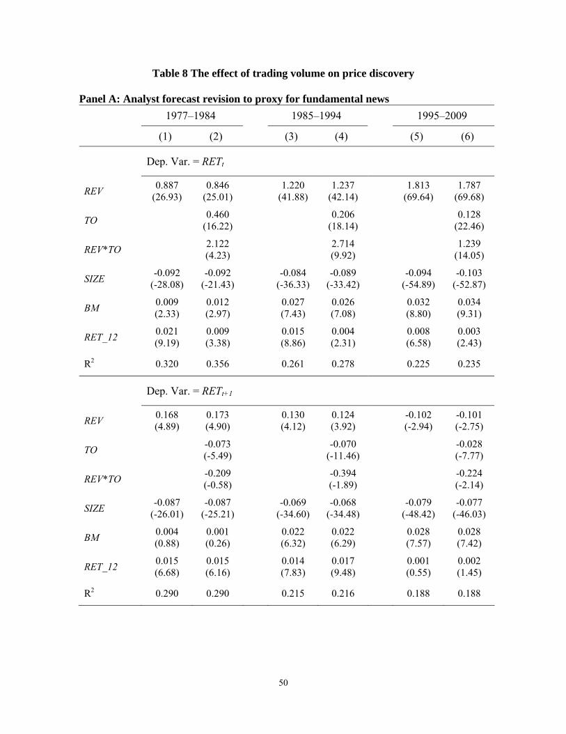
50

Table 8 The effect of trading volume on price discovery

Panel A: Analyst forecast revision to proxy for fundamental news 1977–1984 1985–1994 1995–2009

(1) (2) (3) (4) (5) (6)

Dep. Var. = RETt

REV 0.887 (26.93)

0.846 (25.01)

1.220 (41.88)

1.237 (42.14) 1.813

(69.64) 1.787

(69.68)

TO 0.460 (16.22)

0.206

(18.14) 0.128 (22.46)

REV*TO 2.122 (4.23)

2.714

(9.92) 1.239 (14.05)

SIZE -0.092 (-28.08)

-0.092 (-21.43)

-0.084 (-36.33)

-0.089 (-33.42) -0.094

(-54.89) -0.103

(-52.87)

BM 0.009 (2.33)

0.012 (2.97)

0.027 (7.43)

0.026 (7.08) 0.032

(8.80) 0.034 (9.31)

RET_12 0.021 (9.19)

0.009 (3.38)

0.015 (8.86)

0.004 (2.31) 0.008

(6.58) 0.003 (2.43)

R2 0.320 0.356 0.261 0.278 0.225 0.235

Dep. Var. = RETt+1

REV 0.168 (4.89)

0.173 (4.90)

0.130 (4.12)

0.124 (3.92) -0.102

(-2.94) -0.101 (-2.75)

TO -0.073 (-5.49)

-0.070

(-11.46) -0.028 (-7.77)

REV*TO -0.209 (-0.58)

-0.394

(-1.89) -0.224 (-2.14)

SIZE -0.087 (-26.01)

-0.087 (-25.21)

-0.069 (-34.60)

-0.068 (-34.48) -0.079

(-48.42) -0.077

(-46.03)

BM 0.004 (0.88)

0.001 (0.26)

0.022 (6.32)

0.022 (6.29) 0.028

(7.57) 0.028 (7.42)

RET_12 0.015 (6.68)

0.015 (6.16)

0.014 (7.83)

0.017 (9.48) 0.001

(0.55) 0.002 (1.45)

R2 0.290 0.290 0.215 0.216 0.188 0.188

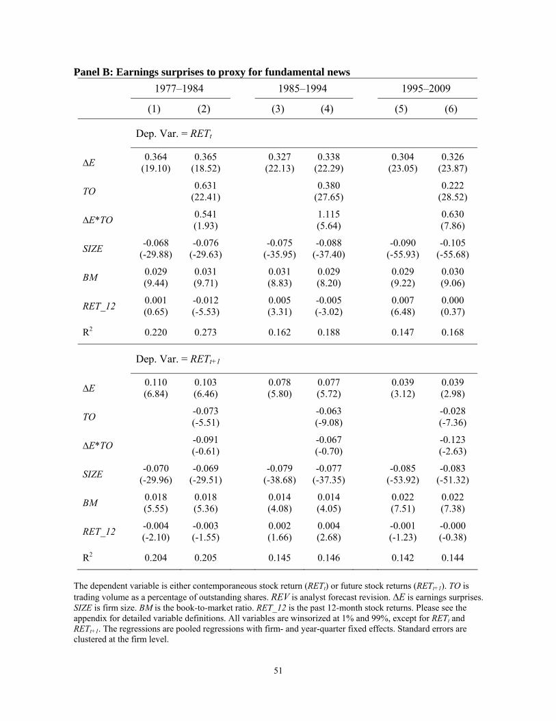
51

Panel B: Earnings surprises to proxy for fundamental news 1977–1984 1985–1994 1995–2009

(1) (2) (3) (4) (5) (6)

Dep. Var. = RETt

∆E 0.364 (19.10)

0.365 (18.52)

0.327 (22.13)

0.338 (22.29) 0.304

(23.05) 0.326

(23.87)

TO 0.631 (22.41)

0.380

(27.65) 0.222 (28.52)

∆E*TO 0.541 (1.93)

1.115

(5.64) 0.630 (7.86)

SIZE -0.068 (-29.88)

-0.076 (-29.63)

-0.075 (-35.95)

-0.088 (-37.40) -0.090

(-55.93) -0.105

(-55.68)

BM 0.029 (9.44)

0.031 (9.71)

0.031 (8.83)

0.029 (8.20) 0.029

(9.22) 0.030 (9.06)

RET_12 0.001 (0.65)

-0.012 (-5.53)

0.005 (3.31)

-0.005 (-3.02) 0.007

(6.48) 0.000 (0.37)

R2 0.220 0.273 0.162 0.188 0.147 0.168

Dep. Var. = RETt+1

∆E 0.110 (6.84)

0.103 (6.46)

0.078 (5.80)

0.077 (5.72) 0.039

(3.12) 0.039 (2.98)

TO -0.073 (-5.51)

-0.063

(-9.08) -0.028 (-7.36)

∆E*TO -0.091 (-0.61)

-0.067

(-0.70) -0.123 (-2.63)

SIZE -0.070 (-29.96)

-0.069 (-29.51)

-0.079 (-38.68)

-0.077 (-37.35) -0.085

(-53.92) -0.083

(-51.32)

BM 0.018 (5.55)

0.018 (5.36)

0.014 (4.08)

0.014 (4.05) 0.022

(7.51) 0.022 (7.38)

RET_12 -0.004 (-2.10)

-0.003 (-1.55)

0.002 (1.66)

0.004 (2.68) -0.001

(-1.23) -0.000 (-0.38)

R2 0.204 0.205 0.145 0.146 0.142 0.144

The dependent variable is either contemporaneous stock return (RETt) or future stock returns (RETt+1). TO is trading volume as a percentage of outstanding shares. REV is analyst forecast revision. ∆E is earnings surprises. SIZE is firm size. BM is the book-to-market ratio. RET_12 is the past 12-month stock returns. Please see the appendix for detailed variable definitions. All variables are winsorized at 1% and 99%, except for RETt and RETt+1. The regressions are pooled regressions with firm- and year-quarter fixed effects. Standard errors are clustered at the firm level.