The Economics of Climate Change in the Dong Nai Delta: Adapting Agriculture to Changes in Hydrologic Extremes1

David Corderi2

1 This draft paper is based on chapter 1 and 2 of the author’s PhD dissertation. The author would like to thank

Jeffrey Williams, Richard Howitt, Jay Lund, Pierre Merel and Michael Springborn for helpful comments and advice. Special thanks to the members of the Southern Institute of Water Resources Planning in Vietnam for kindly providing data and for numerous discussions about the hydrology in the delta. I would also like to thank Claudia Ringler for providing agricultural production data. All errors are my own. Results of the analysis are preliminary, do not cite without permission.

2 Department of Agricultural and Resource Economics, University of California at Davis, One Shields Avenue,

Davis, CA 95616, United States. Telephone: +1 530 400 1023. E-mail: dcorderi@primal.ucdavis.edu.

2

Abstract

The effects of climate change will be particularly felt in the Dong Nai river delta of

Vietnam due to its hydrologic and economic characteristics. Climate change projections suggest

that the delta may be subject to an increasing magnitude of salinity concentration due to changes

in seasonal rainfall patterns. We study the economics of climate change impacts and adaptation

in the delta, with particular attention to changes in hydrologic extremes. Reduction in river flows

during low-flow periods will result in increased salinity levels which will significantly affect

agricultural production in the downstream areas of the delta that are already constrained by

salinity intrusion in the dry season. We integrate these agronomic, hydrologic and economic

aspects of climate change in the delta into a framework that examines optimal cropping patterns

adjustment as well as the optimal timing and location of water infrastructure investments as a

response to increased salinity in the delta. Our results suggest that salinity damages to agriculture

can be alleviated through adjustments in the farming system for a certain range of salinity. Our

analysis also suggests that earlier construction is preferred under scenarios of faster salinity

increases. Finally we find a tradeoff between protecting upstream versus downstream areas in the

delta. For some cases, protecting regions closer to the sea is not economically viable given the

delta’s hydrologic characteristics.

Keywords: climate change adaptation, agriculture, water, cost-benefit analysis, dynamic

programming, Vietnam.

JEL codes: Q54, Q25, Q15.

3

1.- Introduction

Climate change impacts in the water cycle will be strongly felt in the Dong Nai river

delta of Vietnam due to its hydrologic and economic characteristics. We present a study of

climate change impacts and adaptation in the Lower Dong Nai Delta. From an economic

perspective the study area is characterized by its significant contribution to agricultural

production in the region. Rice, sugarcane and vegetables are among the most relevant crops

cultivated in the area and contribute to almost 50 percent of regional GDP. From a hydrologic

perspective, the delta is characterized by having a six month low flow season when rainfall is

very scarce and a flooding season when extreme precipitation and tropical cyclones occur.

Seawater intrusion occurs during the dry season given the relatively flat topography and the low

elevation of the delta’s land with respect to sea level. As a result of this, the accumulation of

salinity in the soils during the dry season is the main limiting factor for agriculture production in

the areas located downstream of the Dong Nai river delta.

The assessment of some the physical impacts of climate change in the delta suggests that

salinity concentration levels will increase due to a combination of higher sea tides and lower

upstream flows in the dry season (Dung Do Duc, 2010). These impacts can have an important

effect on the sustainability of production from agricultural land in the long term. Adapting to

increased salinity may involve changing cropping patterns, adjusting the crop input mix,

constructing new water infrastructure or abandoning land.

We integrate agronomic and hydrologic aspects of climate change in the delta into a

hydro-economic framework that examines the economic desirability and tradeoffs between

4

available adaptation options in the districts located downstream in the delta. The main research

questions that we try to address can be summarized as follows:

How can agricultural production and cropping patterns adapt to increased salinity from an

agro-economic point of view?

What is the interplay between softer adaptation options such as adjustments in cropping

patterns and hard options such as infrastructure investments (sluice gates)?

What is the optimal timing to build protective water infrastructure under different climate

change scenarios?

Where should water infrastructure be built to respond to increasing salinity given the

characteristics of the delta?

Our framework for analysis has two components, a model for agricultural land use, and a

model for water infrastructure investment analysis.

An economic model of agricultural land use is constructed using data available from crop

cost and return studies and land use observations for the area. The model structure and

calibration is similar to the one introduced by Howitt (1995) and later on by Merel and Bucaram

(2010). Our model aims at maximizing the net annual benefit from agricultural production in

each of the delta’s districts taking into account biophysical and economic constraints. An

agronomic function is also incorporated in the model to relate crop yield and salinity levels

following the work by Van Genuchten, M. T., and G. J. Hoffman (1984). When this yield-

salinity relation is introduced in the model the overall impacts of salinity in agricultural

production can be studied in a more robust manner where both agronomic and economic aspects

are integrated. Using mathematical programming techniques the model is able to identify

5

economically feasible adjustments of crop (agriculture land use) and input changes that can

reduce the impact of increased salinity on production. Our model simulations allow us to

parameterize a relationship between the value of annual agricultural production and different

salinity concentration levels.

Secondly, we construct a model for analyzing investments in water infrastructure. The

implicit objective of the model is to minimize land value loss due to salinity in a district by

choosing when and where to invest in water infrastructure. The economic value of agriculture

land is derived using our agriculture model, which relates annual net benefits from agricultural

production to salinity concentration levels. In other words, our model treats agricultural land as

an asset that generates annual profits whose value is depreciating over time due to increased

salinity. Our water infrastructure model has an inter-temporal structure to study investment

planning in a context of long-term climate change adaptation. This allows us to study the optimal

timing profile for building protective structures that can prevent land from loosing value.

The model maximizes the expected net present value of agricultural land, i.e. the

discounted streams of annual agricultural production profits. We formulate the problem as a

dynamic program with one state and one control variable and solve it using the Bellman

equation. Our state variable is salinity level which is based on hydrological simulation results.

Our control variable is a binary variable that represents whether or not a given water

infrastructure is built. The formulation of this problem as a dynamic discrete choice program is

similar to a class of problems that aim to study optimal stopping rules (Dixit and Pindyck, 1994),

i.e. the optimal timing for investment. Using our dynamic model we also study how the optimal

timing for infrastructure investment differs for two climate scenarios that reflect the range of

6

possible future climate outcomes. Finally, we study the economic tradeoffs between protecting

upstream areas versus areas closer to the sea.

This paper begins with a review of the literature related to climate change adaptation in

agriculture and water. Next, we describe the hydrological, agronomic and economic conditions

of the study area in the Dong Nai Delta. The two models and preliminary results are presented in

the following sections. First, we present the mathematical programming model used to study the

effects of salinity in regional agricultural production. Second, we explain the structure of our

dynamic programming model used to evaluate the timing and location of water infrastructure

investments in the delta. We conclude our paper with an interpretation of the results obtained and

possibilities for further extension.

7

2.- Literature Review

The vast majority of studies on the economics of climate change in agriculture and water

have centered on changes in precipitation, temperature or runoff. Most of these studies have

considered changes in average climate characteristics, leaving aside changes in the extremes.

Given the specific characteristics of the Dong Nai delta, i.e., two clearly distinct seasons that

differ greatly, we believe that changes in hydrologic extremes are the most relevant aspects to be

considered for adaptation planning. A reduction in rainfall and consequently upstream freshwater

runoff in the dry-season will exacerbate the current salinity problems caused by seawater

intrusion in the area. Salinity concentration levels in the delta are therefore the proxy that we will

use to study climate changes in seasonal hydrologic extremes. Our study about the economics of

climate change in the delta will focus both on agriculture production and water infrastructure

investments related to the agriculture sector. We review previous approaches used to study these

two aspects of climate change.

2.1.- Agriculture and Climate Change

Our first strand of analysis is the economic study of climate change impacts and

adaptation in agriculture production within the delta. Agricultural production models can be used

for this purpose. Two types of modeling approaches exist, inductive and deductive. We

summarize these two types of approaches below.

Inductive model approaches rely more heavily on a rich data set to provide the data with

which most or all of the parameter values in the model can be estimated from observed behavior

8

using econometric techniques. Econometric models have been widely used to study how changes

in precipitation and temperature affect the value of agriculture production. Earlier models such as

the Ricardian model (Mendelsohn et al. 1994) use a cross-sectional data set to explore how farm

values and net revenues vary across climatic zones. These studies estimate response functions

that are assumed to incorporate optimal adaptation, however there is no clear estimation of

behavioral or operational responses at the farm level. Multinomial logit models have been used

to explicitly estimate adaptation responses such as changes in crop choices or the adoption of

irrigation, see for example Haneman et al. (2005), Seo and Mendelsohn (2006) and Howitt et al.

(2009).

In general, econometric models tend to underestimate the future positive effects of

adaptation. The main reason for this is that the adaptation responses to future climate change

outcomes that lie outside the observed ranges can only be inferred, but not observed. Hence,

adaptation responses having to do with technological improvements cannot be properly studied

in an econometric framework (Adams, 2006).

Deductive models operate with much smaller data sets and use previously estimated

parameters. They involve mathematical programming and assume optimizing behavior that is

calibrated using minimal data. These models can accommodate various types of constraints such

as resource limitations (e.g., land, water), nutrient balance constraints, and other policy relevant

constraints. They can also easily accommodate exogenous information on yields and soil

processes from biophysical models. Previous studies on agriculture and climate change using this

technique have analyzed the effect of climate related crop yield changes (Howitt and Pienaar,

2006) and climate related changes in salinity (Howitt et al., 2009). These studies estimate

9

adaptation responses such as adjusting irrigation, the combination of crops to be grown and the

input mix in response to climate change.

The assumptions made in the construction of these models tend to overestimate the level

of adaptation. In particular, the assumption of no transaction costs or institutional barriers for

reallocating inputs or crops and the assumption of perfect foresight with respect to future climate

conditions can significantly overestimate the mitigation of negative climate impacts.

Given the lack of a sufficiently rich data set for the area of study we will adopt a

deductive approach to study climate change impacts on agricultural production in the delta. We

will also use this approach given its flexibility to incorporate technological improvements on

salt-tolerant crops that are not currently observed in the past but are in the process of being

tested.

2.2.- Water Infrastructure Investments and Climate Change

The second objective of this paper is to study the economic implications of climate

change with respect to water infrastructure investments that are related to agriculture production

in the delta. The main aspects to be considered are the optimal timing of infrastructure

construction as an adaptation investment, taking into account the fixed costs, uncertainty and

irreversibility related to these decisions. In addition to dynamic aspects, spatial considerations of

infrastructure investments are analyzed in order to capture the hydrological complexity of the

delta. In this section we will review previous approaches to studying water infrastructure

investments in the context of climate change and will also give an overview about the literature

on uncertainty and irreversibility.

10

Water infrastructure investments and climate change have previously been studied using

simulation and optimization models. Callaway et al. (2007) explicitly model the expansion of the

water infrastructure system in the context of climate change. Their empirical model considers

structural adaptation measures such as building a dam and non structural measures such as

changes in operations and introducing efficient water market allocations. Their modeling

approach allows them to study the optimal capacity of a reservoir and other structural works such

as water pumps. Even though they consider the interplay between structural and non-structural

measures, the optimal timing and location of the dam as well as uncertainty aspects are not fully

considered in their study.

Fisher and Rubio (1997) consider uncertainty and irreversibility in a theoretical

framework applied to investments in infrastructure related to water storage capacity. They find

that increases optimal water storage capacity increases with greater variance of water resource

availability. Their study also finds that there is a range of inaction for investments in

infrastructure when there is a high cost for reversing investments.

Block and Strzepek (2007) develop a model to assess investments in dam development

for hydropower and irrigation purposes in a context of future climate change. They consider the

implications of climate extremes for the analysis of the potential net benefits of infrastructure

development. Another important aspect of their modeling framework is the sequential nature of

various dam constructions along the Nile River. However, their model objective is to simulate

future conditions, i.e., their focus is to assess the economic performance of a given infrastructure

investment plan along the river under climate change conditions. The authors do not attempt to

study what would be the optimal number and size of dams in the river given climate change

conditions.

11

Lund et al. (2006) and Medellin et al. (2008) develop an optimization model that can

evaluate the additional needs and value of increased water storage or infrastructure expansion

under prolonged drought conditions due to climate change. The model optimizes both water

allocations and the operation of water facilities to study different adaptation options given a set

of infrastructure and physical constraints. The model considers broad mix of adaptation options

such as system re-operation, conjunctive use, water reuse and desalination, water markets and

water conservation. Although the model does not explicitly address the optimal timing of

infrastructure investment, it does have the potential to size optimal investments in infrastructure

as well as their location.

Zhu et al. (2007) address the optimal timing of infrastructure investment in a study flood

protection and adaptation of floodplains to climate change and urbanization. The authors use an

optimization model. The focus is on levee design in a river basin as a long term adaptation

option. The dynamic programming model maximizes the value of the floodplain by choosing

levee setback and height, taking into account the costs and the benefits associated with those

decisions as well as the probability of flooding. The authors find the optimal timing profile of

changes in levee height and setback for a given set of climate change scenarios.

Finally, the theoretical literature on uncertainty, irreversibility and investment timing is

summarized by Dixit and Pyndick (1994). Wright and Erickson (2003) review this literature and

consider its application to climate change adaptation. The authors develop an option value

framework to study the optimal timing for adaptation responses using an optimal stopping

model. Their modeling study is not based on empirically estimated parameters; however their

work constitutes a good illustration of the additional aspects to be considered when it comes to

water infrastructure investments and climate change uncertainty.

12

The water infrastructure investment model developed in this paper uses an optimization

framework as opposed to simulation. The optimization model uses dynamic programming to find

the optimal timing and location of infrastructure construction. The initial model specification

considers a range of extreme hydrologic scenarios under a closed loop.

2.- The Dong Nai Delta: Hydrology, Agriculture and Climate Change.

The Dong Nai River Basin (DNRB) is the largest national river basin and the economic

center of the country in southern Vietnam. The delta is situated in the lowland areas of the basin.

The Lower Dong Nai Delta includes 4 provinces and Ho Chi Minh City as can be seen in table 1.

Both HCMC and BR-VT are important urban and industrial centers respectively whereas Long

An and Tay Ninh have important agricultural production areas. Total population in the area

amounts to more than 9 million inhabitants. Agriculture production is highly diversified, with

products ranging from staple crops like rice, to raw materials for the local industry such as

sugarcane, to high-valued crops like vegetables and fruits.

Table 1: Economic Indicators for the Provinces in the Lower Dong Nai River Delta

Province

Land Area

2007

Gross Irrigated Area

2007

Population

2007

GDP

2007

Share Agriculture GDP 2007

(ha) (ha) (‘000) (M USD) (%)

HCMC 209,505 72,482 6,347 6254 4

Long An 188,153 151,246 1,430 724 54

Tay Ninh 402,812 220,635 1,053 413 46

BR-VT 190,000 30,057 947 4456 5

TOTAL 990,470 474,420 9,777

Reference: Land area: Sub-NIAPP; Gross irrigated area: adjusted from SIWRP; Population and GDP: various statistical yearbooks from GSO.

13

The Lower Dong Nai Delta has 3 major rivers: the Dong Nai mainstream, the Sai Gon,

and the Vam Co Dong system that joins the Dong Nai just before the outlet into the East Sea

(figure 1). Two reservoirs are located upstream of the Sai Gon and Dong Nai rivers, Dau Tieng

and Tri An. Dau Tieng is actually the largest irrigation reservoir in Vietnam.

The delta area possesses abundant water resources; however, the delta is subject to annual

flooding in the wet season and salinity intrusion in the dry season (Ringler and Huy 2004). The

area is therefore more vulnerable to hydrologic extremes than to changes in average hydrology.

Figure 1: Lower Dong Nai Delta

Source: SIWRP (2009)

14

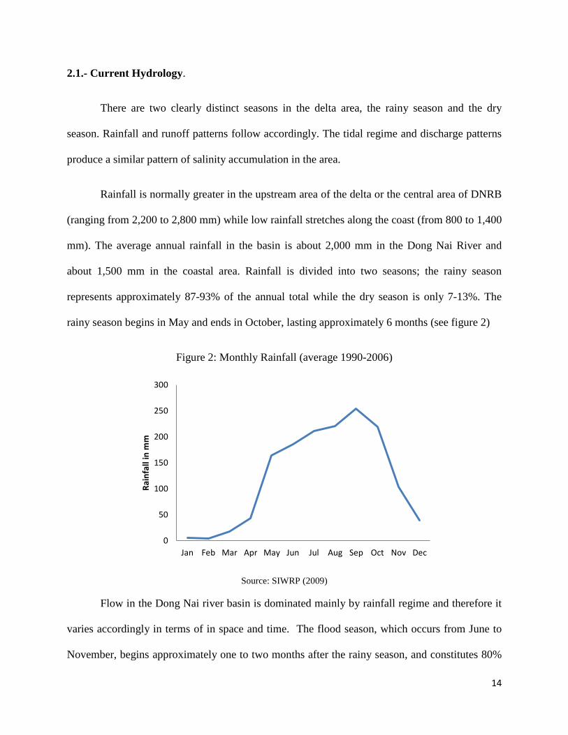
2.1.- Current Hydrology.

There are two clearly distinct seasons in the delta area, the rainy season and the dry

season. Rainfall and runoff patterns follow accordingly. The tidal regime and discharge patterns

produce a similar pattern of salinity accumulation in the area.

Rainfall is normally greater in the upstream area of the delta or the central area of DNRB

(ranging from 2,200 to 2,800 mm) while low rainfall stretches along the coast (from 800 to 1,400

mm). The average annual rainfall in the basin is about 2,000 mm in the Dong Nai River and

about 1,500 mm in the coastal area. Rainfall is divided into two seasons; the rainy season

represents approximately 87-93% of the annual total while the dry season is only 7-13%. The

rainy season begins in May and ends in October, lasting approximately 6 months (see figure 2)

Figure 2: Monthly Rainfall (average 1990-2006)

Source: SIWRP (2009)

Flow in the Dong Nai river basin is dominated mainly by rainfall regime and therefore it

varies accordingly in terms of in space and time. The flood season, which occurs from June to

November, begins approximately one to two months after the rainy season, and constitutes 80%

0

50

100

150

200

250

300

Jan Feb Mar Apr May Jun Jul Aug Sep Oct Nov Dec

Rain

fall

in m

m

15

of the total annual flow. The dry season lasts over six months from December to May, with

lowest flow in March or April or even in May. Monthly flow records indicate highest totals in

the July-September months (see figure 3).

Figure 3: Monthly Runoff (1990-2006)

Source: SIWRP (2009)

Salinity is already a problem due to the delta’s hydrologic and geomorphologic

characteristics (see figure 4). The lower Dong Nai delta is a low-lying area with a complex

branched and looped river network and is strongly affected by tides from the East Sea in the

Pacific Ocean. The tidal amplitude is very large, and may reach up to 3.5-4.0 m along the coast.

Due to the large amplitudes of the tide and the low riverbed slopes, the tide propagates from the

sea to the river mouth and then further into the rivers and canals. Under natural conditions, the

tide affects the water level up to the Tri An waterfall foot in the Dong Nai River, 132.8 km from

the sea, to the Dau Tieng dam site in the Sai Gon River, 184.4 km from the sea, and to the

Cambodia border in the East Vam Co River, 208 km from the sea.

0

500

1000

1500

2000

Jan Feb Mar Apr May Jun Jul Aug Sep Oct Nov Dec

Surf

ace

flow

(m3)

AverageMaxMin

16

Figure 4: Current Salinity Area Map

Source: SIWRP (2008)

Salinity dynamics follow from rainfall and river flow patterns. Salinity levels reach their

peak during the last months of the dry season which coincide with the periods of lowest flow,

normally in April or even in May. The rainy season decreases salinity build-up in the delta’s land

for almost six months (see figure 5).

17

Figure 5: Seasonal Salinity Dynamics

The spatial distribution of salinity concentration in lands follows from the delta’s

morphologic characteristics. Downstream areas that are closer to the sea such as the Can Duoc

districts are subject to higher salinity concentrations throughout the dry season (see figure 6)

Figure 6: Spatial Salinity Dynamics

0

2

4

6

8

10

12

14

Jan Feb Mar Apr May Jun Jul Aug Sep Oct Nov Dec

Soil

Salin

ity (d

S/m

)

0

2

4

6

8

10

12

14

16

Jan Feb Mar Apr May Jun

Soil

Salin

ity (g

/l)

Can Duoc

Tan Tru

Ben Luc

18

2.2.- Agriculture in the study area.

The area of study has been selected based on two factors, the projections on the spatial

extent of future salinity increases and the relative importance of agriculture in the regional

economy. Five downstream districts belonging to Long An province have been selected (see

figure 7). The districts selected are Ben Luc, Tan Tru, Can Guioc, Can Duoc and Chau Thanh.

These study area is smaller than Lower Dong Nai Delta area; however, it covers more than 85

percent of the area and agricultural production affected by seawater intrusion. We believe that it

is also a good representation for the water infrastructure model developed later on since more

than 70 percent of the infrastructure investment plans refer to that area.

Figure 7: Map of Administrative Boundaries for Selected Districts of Study

Agricultural production is one of the main economic activities in the district selected.

More than 70 percent of land is dedicated to agriculture. Annual crops are separated by season

19

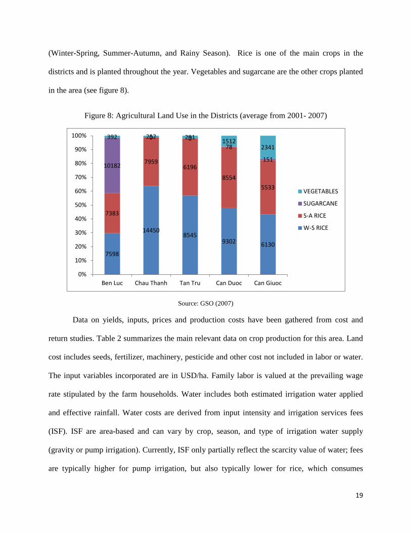
(Winter-Spring, Summer-Autumn, and Rainy Season). Rice is one of the main crops in the

districts and is planted throughout the year. Vegetables and sugarcane are the other crops planted

in the area (see figure 8).

Figure 8: Agricultural Land Use in the Districts (average from 2001- 2007)

Source: GSO (2007)

Data on yields, inputs, prices and production costs have been gathered from cost and

return studies. Table 2 summarizes the main relevant data on crop production for this area. Land

cost includes seeds, fertilizer, machinery, pesticide and other cost not included in labor or water.

The input variables incorporated are in USD/ha. Family labor is valued at the prevailing wage

rate stipulated by the farm households. Water includes both estimated irrigation water applied

and effective rainfall. Water costs are derived from input intensity and irrigation services fees

(ISF). ISF are area-based and can vary by crop, season, and type of irrigation water supply

(gravity or pump irrigation). Currently, ISF only partially reflect the scarcity value of water; fees

are typically higher for pump irrigation, but also typically lower for rice, which consumes

7598

14450 8545

9302 6130

7383

7959 6196

8554 5533

10182

0 0 78

151

392 252 291 1512 2341

0%

10%

20%

30%

40%

50%

60%

70%

80%

90%

100%

Ben Luc Chau Thanh Tan Tru Can Duoc Can Giuoc

VEGETABLES

SUGARCANE

S-A RICE

W-S RICE

20

relatively more water (Ringler, 2004). It is also worth noting that districts located downstream

have on average a higher cost of production due to salinity conditions.

Table 2: Crop Prices, Input Use and Yields

Crop Price Yield Land Cost Irrigation Water Labor

(USD/mt) (mt/ha) (USD/ha) (mm) (USD/ha)

W-S Rice 135 3.78 69 (112) 1102 (1203) 38 (71)

S-A Rice 130 3.3 79 (101) 679 (785) 40 (65)

Sugar Cane 24 48.7 68 (183) 1983 (2291) 57 (86)

Vegetables 211 4.17 54 (81) 502 (584) 48 (73)

Reference: various data sources, Sub-NIAPP, Ringler, SIWRP, and agricultural census. Exchange rate is assumed to be 1USD ~19,000 VND. Numbers in parenthesis correspond to districts located closer to the sea.

2.3.- Climate change projections

Climate change scenarios of future salinity concentration levels have been produced for

the Dong Nai Delta following from earlier work conducted by SIWRP and the World Bank.

Projections of changes in temperature and precipitation were introduced into a rainfall-runoff

model (NAM) to produce upstream flow projections. The combination of flow projections with

different scenarios of sea level rise (MONRE, 2009) was used in a hydro-dynamic model (MIKE

11) to produce salinity maps in the delta. Climate projections were selected from an ensemble of

climate models that simulate the A2 emissions scenario of the IPCC FAR(2007). The main goal

of climate change projections was to examine the upper and lower boundaries in the range of

possible climate scenarios. Two climate model projections were selected according to a moisture

index that ranked model outputs according to precipitation and temperature. A wet scenario was

21

associated to the Goddard Institute for Space Studies (GISS –ER) climate model and a dry

scenario was associated to the Institut Pierre Simon Laplace (ISPL-CM4) climate model.

Overall, climate change scenarios suggest a decrease in runoff in the dry period which,

combined with sea level rise leads to increases in salinity concentration over time. Areas closer

to the sea tend to have greater increases in salinity levels. These salinity projections assume that

there are no new water infrastructures in place. Figure 9 provides a good overview of the spatial

distribution of salinity levels in 2050.

Figure 9: Projected average salinity for 2050 (dry scenario)

Source: SIWRP (2010)

3.- Economic Model of Agriculture Production

An economic model of agricultural land use is constructed using data available from crop

cost and return studies and land use observations for the area. The model aims at maximizing the

net annual benefit from agricultural production in each of the delta’s districts taking into account

22

biophysical and economic constraints. This model is used to estimate the effect of increased

salinity on crop production in the area. The direct economic impacts of salinity accumulation are

reflected in net agricultural profit loss. Changes in cropping patterns (intensive and extensive

margin) due to salinity accumulation are also estimated within the model. It is also assumed that

the region is a price-taker in agricultural markets; hence prices are assumed to be exogenous in

the model. Rainfed agriculture is not considered in the model given that irrigated crop production

is the dominant agricultural industry in the districts of study.

Estimation takes place within the context of positive mathematical programming (Howitt

1995), as a self-calibrating three-step procedure. First step, a linear program for profit

maximization is solved. In addition to the traditional resource and non-negativity constraints a

set of calibration constraints is added to restrict land use to observed values. The second step is

parameterization of a quadratic cost function and the production function itself from the first

order conditions. LaGrange multipliers from the binding calibration constraints in the first step

are used to estimate slope and intersect of the average cost function. A third and last step

incorporates the parameterized cost functions into a non-linear profit maximization program,

with constraints on resources only. Salinity effects are incorporated by calculating the impact of

reduction in crop yields due to salinity.

The economic effects of salinity changes are estimated by iterating the optimization

algorithm for different salinity levels and measuring the costs of changes in cropping

combinations, crop yields, and areas with respect to the base case.

23

3.1.- The Objective Function The economic model proposed here is based on a class of models called Positive

Mathematical Programming or PMP (Howitt, 1995), widely used in applied research and policy

analysis. It is assumed that farmers in each district within the Dong Nai delta seek to maximize

net revenue derived from their farming activities in a given year. Therefore, the backbone of the

analytical model is an objective function that explicitly sets out to maximize profits. That is:

max𝑋≥0

���𝑝𝑖 ∗ 𝑓𝑔𝑖 − �𝜔ℎ ∗ 𝑋𝑔𝑖ℎ −�(𝛼𝑔𝚤� ∗ 𝑋𝑔𝑖ℎ𝑖

+12∗

ℎ

𝛾𝚤𝑔� ∗ 𝑋𝑔𝑖𝑙𝑎𝑛𝑑2 𝑖

� Eq. 1𝑔

The first term on equation 1 represents gross revenue, where pi is the output price of the

perennial or annual crop i, each of which is produced according to a production function fgi. Xgih,

described in more detail in the next section, is the matrix of i perennial and annual crops, and h

agricultural inputs, and sets the input requirements for producing all crop products. Inputs

include: land, labor and water. The subscript g refers to the regions of study.

The cost to produce a unit of crop i is defined by two remaining terms: the first term is

the market price of the inputs, ωh, multiplied by the quantity of inputs used ihX ; and the second

term, in parenthesis, is the implicit cost associated with land allocation. It has a quadratic

specification with parameters iα and 𝛾𝑖 and captures the increasing marginal cost associated

with allocating larger amounts of land to a given crop. As a given farmer allocates increasing

amounts of land to a specific crop, the new land may be of inferior quality or not as suitable to

grow that particular crop. More generally, this term captures non-linear effects that may enter

into the decision-maker’s problem and that are not directly observable or measurable causing

costs to rise non-linearly with area.

24

The original objective function is then adjusted to better capture seasonality in the

farming system. Equation 1 will be used to represent the objective function for each crop rotation

(winter-spring and summer autumn). Additional constraints will reflect the availability of

resources for each season as well as the rotational constraints on perennial crops.

3.2- The Production Function

The production function fgi(Xgih), provides an estimate of output produced in district g by

an existing set of inputs h for each cropping activity i. The functional form used for f is a

constant elasticity of substitution (CES) and the parameters are calibrated as in Howitt (2006).

Elasticity of substitution is assumed to vary by crop but not by region. The specification of the

generalized CES production function is:

𝑓𝑔𝑖 = 𝐴𝑔𝑖 ��𝛽𝑔𝑖ℎ𝑋𝑔𝑖ℎ𝜌𝑔𝑖

ℎ

�

𝜖𝑖𝜌𝑔𝑖

Eq. 2

where Ai represents the area share parameter, and βih are the production function parameters;

σσγ 1−

= , σ is the elasticity of substitution among inputs; and εi is the returns-to-scale

parameter.

3.3 Model Calibration and Parameterization

The first step in PMP is devoted to obtaining marginal values for the calibration

constraints to parameterize a quadratic cost function in the second step. The linear program with

calibration constraints has as its explicit objective the maximization of net revenue using land in

each of the two crop rotations as the decision variable and is as follows:

25

max𝑥𝑔𝑖1 ≥0, 𝑥𝑔𝑖

2 ≥0���𝑝𝑔𝑖1 ∗ 𝑦�𝑔𝑖1 ∗ 𝑋𝑔𝑖1 − �𝜔𝑖ℎ

1 ∗ 𝑎𝑔𝑖ℎ1 ∗ 𝑋𝑔𝑖ℎ1

𝑖𝑖

�𝑔

+ ���𝑝𝑔𝑖2 ∗ 𝑦�𝑔𝑖2 ∗ 𝑋𝑔𝑖2 − �𝜔𝑖ℎ2 ∗ 𝑎𝑔𝑖ℎ2 ∗ 𝑋𝑔𝑖ℎ2

𝑖𝑖

�𝑔

Eq. 3

subject to seasonal and district-level resource constraints:

⎩⎪⎨

⎪⎧ ��𝑋𝑔𝑖1 = 𝐵𝑙𝑎𝑛𝑑

𝑖𝑔

��𝑋𝑔𝑖2

𝑖𝑔

= ��𝑋𝑔𝑖1

𝑖𝑔

𝑋𝑔,𝑠𝑢𝑔𝑎𝑟1 = 𝑋𝑔,𝑠𝑢𝑔𝑎𝑟

2

Eq. 4

��𝑎𝑔𝑖,𝑙𝑎𝑏𝑟 ∗ 𝑋𝑔𝑖,𝑙𝑎𝑏𝑟 = 𝐵𝑙𝑎𝑏𝑟

𝑖𝑔

∀ 𝑟 ∈ (1,2) Eq. 5

��𝑎𝑔𝑖,𝑤𝑎𝑡𝑟 ∗ 𝑋𝑔𝑖,𝑤𝑎𝑡𝑟 = 𝐵𝑤𝑎𝑡𝑟

𝑖𝑔

∀ 𝑟 ∈ (1,2) Eq. 6

𝑋𝑖𝑙𝑎𝑛𝑑𝑟 ≤ 𝑋�𝑖𝑙𝑎𝑛𝑑𝑟 Eq. 7

where in Eq. 3 pi is defined as before, ŷ is the yield per hectare of land dedicated to crop i, ωih is

the unit cost of input h used in the production of crop i, and aih are inputs per hectare

iland

ihX

X . Bland, Blab and Bwat reflect the total availability of land, labor and water,

respectively. The superscript r indicates whether it is the first rotation (1) or the second rotation

(2) which correspond to the winter-spring season or the summer autumn season. Eq. 4 contains

the seasonal constraints. 𝑋𝑔𝑖1 is the amount of land dedicated to region i in region g under the

winter spring season (rotation 1). The total amount of land dedicated to crops per season must be

equal to 𝐵𝑙𝑎𝑛𝑑, in our case, the total amount of crop land in season 2 is less than cropland in

26

season 1 due to increased salinity, therefore there is also fallow land during season 2 (summer

autumn). The last restriction of equation 4 ensures that perennial crops (sugarcane) are properly

taken into account.

In Eq. 7, 𝑋�𝑖𝑙𝑎𝑛𝑑𝑟 is the total amount of land allocated to crop i in season r that is observed

by researchers; this constraint prevents specialization and preserves observed crop allocation

patterns while estimating shadow values of limited or non-marketed inputs. Notice that although

the shadow values associated with the fixed inputs such as land, labor, and water may change

from farmer to farmer, they are not crop specific. However, the Lagrange multiplier associated

with Eq. 7 is both region- and crop-specific.

2.4 Estimation of Production Function Parameters

Estimation of the full set of parameters for the production function with 4 inputs in Eq. 2

requires each crop i to be parameterized in terms of 4 parameters ihβ , one for the return-to-scale

parameter iε and the crop specific parameter Ai in Eq. 2.

In this paper we follow an analytical rather than an econometric method in which the

parameters are calculated using the economic optimality conditions for the use of each input and

some prior values for some key parameters such as the elasticity of substitution. These

conditions seek maximization by setting the value of the marginal product of each input equal to

its unitary cost. In which the former is defined by its output price multiplied by the derivative of

the production function (Eq. 2) with respect to each input. For the unconstrained inputs, the

unitary cost is simply their market price; for the constrained inputs, each unitary cost is the sum

of their purchase prices and their respective shadow values, , , land Labor SurfaceWaterλ λ λ .

Regarding the value of land, however, in addition to the market and shadow prices, the

27

calibration constraint represented by Eq. 7 further increases the value of this fixed input. In other

words, the true marginal cost associated with land allocation to the ith crop is the sum of: 1) the

market price of land; 2) the shadow value of land, λLand; and 3) landiλ .

By algebraically manipulating the optimality equations we reach expressions for each of

the parameters ihβ , and Ai , iα and 𝛾𝑖 in Eq. 1 as a function of values on input prices, output

prices, and input quantities. For this exercise we assume constant returns to scale for all crops (

1== εε i ) and a priori value of 0.4 for the elasticities of substitution (σi). We perform exact

calibration of the elasticities using the method proposed by Merel and Bucaram (2010). An

appendix containing the derivation and calculation of elasticities and parameters ihβ , and Ai, as

well as iα and 𝛾𝑖 of Eq. 1 may be requested to the author .

2.5 Economic Simulation Model

Equation 8 uses the parameterized CES production function 𝑓𝑔𝑖𝑟 to find the optimal set of

inputs that maximizes net revenue:

max𝑥𝑔𝑖1 ≥0, 𝑥𝑔𝑖

2 ≥0���𝑝𝑔𝑖1 ∗ 𝑓𝑔𝑖1 ∗ 𝑋𝑔𝑖1

𝑖𝑔

− ��(𝜔𝑖ℎ1 ∗ 𝑋𝑔𝑖ℎ1 + �̂�𝑔𝑖𝑙𝑎𝑛𝑑1 ∗ 𝑋𝑔𝑖𝑙𝑎𝑛𝑑1

ℎ

+ 12∗ 𝛾�𝑔𝑖 ∗ �𝑋𝑔𝑖𝑙𝑎𝑛𝑑1 �

2

𝑖

)�

+ ���𝑝𝑔𝑖2 ∗ 𝑓𝑔𝑖2 ∗ 𝑋𝑔𝑖2

𝑖𝑔

− ��(𝜔𝑖ℎ2 ∗ 𝑋𝑔𝑖ℎ2 + �̂�𝑔𝑖2 ∗ 𝑋𝑔𝑖𝑙𝑎𝑛𝑑2

ℎ

−12∗ 𝛾�𝑔𝑖 ∗ �𝑋𝑔𝑖𝑙𝑎𝑛𝑑2 �

2

𝑖

� Eq. 8

subject to technological constraints as well as resource availability constraints both at regional

and seasonal level:

28

𝑓𝑔𝑖𝑟 = 𝑦𝑟𝑒𝑑𝑔𝑖 𝐴𝑔𝑖 ��𝛽𝑔𝑖𝑗𝑥𝑔𝑖𝑗𝜌𝑔𝑖

3

𝑗=1

�

𝜖𝑔𝑖𝜌𝑔𝑖

⎩⎪⎨

⎪⎧ ��𝑋𝑔𝑖1 = 𝐵𝑙𝑎𝑛𝑑

𝑖𝑔

��𝑋𝑔𝑖2

𝑖𝑔

= ��𝑋𝑔𝑖1

𝑖𝑔

𝑋𝑔,𝑠𝑢𝑔𝑎𝑟1 = 𝑋𝑔,𝑠𝑢𝑔𝑎𝑟

2

��𝑎𝑔𝑖,𝑙𝑎𝑏𝑟 ∗ 𝑋𝑔𝑖,𝑙𝑎𝑏𝑟 = 𝐵𝑙𝑎𝑏𝑟

𝑖𝑔

∀ 𝑟 ∈ (1,2)

��𝑎𝑔𝑖,𝑤𝑎𝑡𝑟 ∗ 𝑋𝑔𝑖,𝑤𝑎𝑡𝑟 = 𝐵𝑤𝑎𝑡𝑟

𝑖𝑔

∀ 𝑟 ∈ (1,2)

In equation 8, 𝑓𝑔𝑖𝑟 is characterized by the production function defined by the parameters

obtained in the previous subsection. The second term in the equation has now the PMP calibrated

cost function. The production function includes now the term yredgi which represents the yield

reductions from van Genuchten and Hoffman (1984) and is detailed in equation 9 below. Ymaxgi

is the maximum average yield of crop i in region g; cgi is the salinity in the region; c50gi is the

salinity at which the yield is reduced by 50% and is obtained from field experiments; 𝜏 is an

empirical constant.

𝑦𝑟𝑒𝑑𝑔𝑖 =𝑌𝑚𝑎𝑥𝑔𝑖

1 + �𝑐𝑔𝑖𝑐50𝑔𝑖

�𝜏 Eq. 9

2.6.- Simulation Results

We simulate increases in salinity using the calibrated model and are able to parameterize

a salinity damage function to agriculture. Preliminary results suggest that annual agricultural

production losses due to increased salinity follow a non-linear pattern. The different districts

present different responses to salinity increases see figure 10.

29

Figure 10: Annual production value as a function of salinity

From an economic point of view, agricultural production can adapt to increased salinity

by switching from low value-low salt tolerant crops such as rice to high value-high tolerant crops

such as sugarcane or vegetables for a certain range of salinity levels (see figure 11).

Figure 11: Crop mix as a function of salinity

0

20,000

40,000

60,000

80,000

100,000

120,000

0 2 4 6 8 10 12 14 16 18 20

mill

ion

VND

Salinity Level (g/l)

Region 1

Region 2

Region 3

Region 4

Region 5

0

2,000

4,000

6,000

8,000

10,000

12,000

1 3 5 7 9 11 13 15 17 19 21 23 25 27 29 31

Hec

tare

s of L

and

Salinity Level (g/l)

W-S Rice

S-A Rice

Sugarcane

Vegetables

30

4.- Water Infrastructure Investment Model.

A water infrastructure investment model is used to study the optimal timing and location

of sluice gates construction in the delta. The implicit objective of the model is to minimize land

value loss due to salinity by choosing when and where to construct sluice gates in the districts.

The economic value of agriculture land is derived using our agriculture land use model, which

relates annual net benefits from agricultural production to salinity concentration levels. We

approximate the net benefit from land in a given year t as a function that is quadratic in salinity

(equation 9). 𝑆𝑡 is the state variable representing the level of salinity at time t. The value of

agricultural land will also depend on whether the sluice gate is built. 𝑋𝑡 is a binary control

variable representing the decision to build, a value of 1 means that we build a sluice gate in the

district.

𝑓(𝑆𝑡,𝑋𝑡) = 𝑎 − 𝑏 ∗ 𝑆𝑡 − 𝑐 ∗ 𝑆𝑡2 � 𝑓(𝑆𝑡, 0) = 𝑎 − 𝑏 ∗ 𝑆𝑡 − 𝑐 ∗ 𝑆𝑡2 𝑓(𝑆𝑡, 1) = 𝑎 − 𝑏 ∗ 𝛿 − 𝑐 ∗ 𝛿2 − 𝑑

Eq. 9

The parameter 𝑎 represents agricultural land production under current salinity levels and

the parameters 𝑏 and 𝑐 are coefficients used to construct a quadratic salinity loss function. When

a sluice gate is built, the districts incurs in a onetime fixed cost, 𝑑.

The transition of salinity levels from year to year is as follows (equation 10). Salinity

increases by 𝜇 percent each year if no sluice gate is constructed and can be stabilized at a level 𝛿

which follows from previous studies in the area such as Nguyen (2009). The transition equation

is as follows:

𝑔(𝑆𝑡,𝑋𝑡) � 𝑔(𝑆𝑡, 0) = (1 + 𝜇) ∗ 𝑆𝑡

𝑔(𝑆𝑡, 1) = 𝛿 Eq. 10

31

We start with a deterministic, discrete space and discrete control program, assuming a

planning period of 40 years. The model maximizes the expected net present value of agricultural

land, i.e. the discounted streams of annual agricultural production profits. The problem is

formulated as a dynamic program with one state and one control variable using the Bellman

equation as follows:

𝑉(𝑠) = max𝑋𝑡=0,1{𝑓(𝑠) + 𝛽 ∗ 𝑉(𝑠 + 1),𝑓(𝑓) − 𝑑 + 𝛽 ∗ 𝑉(𝑓)} Eq. 11

This model will be used to study several aspects of sluice gate construction in the delta.

First we study the effects of uncertainty on the decision to build sluice gates by examining the

optimal timing profile of construction under two climate scenarios that reflect the range of

possible future climate outcomes. Second, we study the economic tradeoffs between protecting

upstream areas versus areas closer to the sea by building a multi-region investment model that

incorporates district-specific crop productivity and infrastructure cost.

4.1.- One region model simulation results

We numerically solve for the optimal policy rule, i.e., the timing profile of sluice gate

construction and simulate the optimal state path using matlab version 7.10.

Table 3: Parameter Values (Base Case)

Parameter Value

discount rate () 0.95

a (net benefit from land) 150

b (linear salinity damage coefficient) 0.5

c (quadratic salinity damage coefficient) 0.04

d (fixed cost of infrastructure investment) 100

𝜇 (salinity drift rate) 0.05

f (constant salinity value after infrastructure is built) 6

32

T (number of periods) 50

Our first experiment is to examine the implications of uncertain climate change scenarios

in the decision to construct sluice gates. In order to do this we construct two extreme scenarios, a

“wet” scenario where salinity does not build up as fast (base case) and a “dry” scenario where

salinity increases faster (8 percent). We then compare the optimal timing of investment under

these scenarios assuming that the decision maker is risk-neutral. Simulation results suggest that

from an economic point of view it is optimal to build sluice gates earlier under a dry scenario

(see figure 12).

Figure 12: Model simulations comparison of wet and dry scenario

(a) Optimal Timing Sluice Gate Investment (b) Optimal Salinity Path

4.2.- Multi-region model simulation results

The one region model is extended to a three region model to study the economics of

sluice gate location along an interlinked hydrologic system. A tradeoff arises between protecting

additional areas closer to the sea and the additional cost of sluice gate construction. Building a

sluice gate closer to the sea implies a higher cost given the fact the river section to be covered is

0

1

1 4 7 10 13 16 19 22 25 28 31

(0=w

ait;

1=bu

ild)

Years

Wet Scenario Dry Scenario

68

1012141618

1 3 5 7 9 11 13 15 17 19 21 23 25

Salin

ity

Years

Wet Scenario Dry Scenario

33

greater, see figure 13, at the same time the amount of agricultural land that is protected is also

greater. However, the additional benefit from protecting downstream decreases as we move

closer to the sea due to the fact that agricultural productivity is already facing greater salinity

impacts.

Figure 13: Cross Section of East Vam Co River (downstream-upstream)

Source: SIWRP (2009)

The model structure is similar to that of the one region model. Region specific land value

functions are developed for the three regions, see equation 12. The value of land to be considered

now includes three regions as opposed to only one region (equation 13); an additional constraint

ensures that productivity from land cannot be negative (equation 14). It is worth pointing out that

our state space is now composed of salinity in region i (𝑆𝑖𝑡) and our control space includes i+1,

i.e., sluice gate location and the possibility of no protection at all.

𝑓𝑖(𝑆𝑖𝑡,𝑋𝑖𝑡) = 𝑎𝑖 − 𝑏𝑖 ∗ 𝑆𝑖𝑡 − 𝑐𝑖 ∗ 𝑆𝑖𝑡2 Eq.12

𝐹(𝑆𝑖𝑡,𝑋𝑖𝑡) = ∑ 𝑓𝑖(𝑆𝑖𝑡,𝑋𝑖𝑡)3𝑖=1 Eq. 13

𝑓𝑖(𝑆𝑖𝑡,𝑋𝑖𝑡) = max{𝑓𝑖(𝑠𝑖𝑡,𝑥𝑖𝑡), 0} Eq. 14

34

Our global land value function is as a function of regional salinity and sluice gate

location as follows:

𝐹(𝑆𝑖𝑡,𝑋𝑖𝑡) =

⎩⎨

⎧𝐹(𝑆𝑖𝑡; 𝑋1𝑡 = 0,𝑋2𝑡 = 0,𝑋3𝑡 = 0) = 𝑓1(𝑆1𝑡) + 𝑓2(𝑆2𝑡) + 𝑓3(𝑆3𝑡)𝐹(𝑆𝑖𝑡; 𝑋1𝑡 = 1,𝑋2𝑡 = 0,𝑋3𝑡 = 0) = 𝑓1(𝛿) + 𝑓2(𝛿) + 𝑓3(𝛿) − 𝑑1𝐹(𝑆𝑖𝑡; 𝑋1𝑡 = 0,𝑋2𝑡 = 1,𝑋3𝑡 = 0) = 𝑓1(𝑆1𝑡) + 𝑓2(𝛿) + 𝑓3(𝛿) − 𝑑2𝐹(𝑆𝑖𝑡; 𝑋1𝑡 = 0,𝑋2𝑡 = 0,𝑋3𝑡 = 1) = 𝑓1(𝑆1𝑡) + 𝑓2(𝑆2𝑡) + 𝑓3(𝛿) − 𝑑3

The state transition is as follows:

𝑔(𝑆𝑖𝑡,𝑋𝑖𝑡)

=

⎩⎨

⎧𝑔(𝑆𝑖𝑡; 𝑋1𝑡 = 0,𝑋2𝑡 = 0,𝑋3𝑡 = 0) => 𝑆𝑖𝑡 = (𝑟𝑖 ∗ 𝑆𝑡) ∗ (1 + 𝜇)

𝑔(𝑆𝑖𝑡; 𝑋1𝑡 = 1,𝑋2𝑡 = 0,𝑋3𝑡 = 0) => 𝑆𝑖𝑡 = 𝛿 𝑔(𝑆𝑖𝑡; 𝑋1𝑡 = 0,𝑋2𝑡 = 1,𝑋3𝑡 = 0) => 𝑆1𝑡 = (𝑟1 ∗ 𝑆𝑡) ∗ (1 + 𝜇); 𝑆𝑖𝑡 = 𝛿 ∀𝑖 = 2,3𝑔(𝑆𝑖𝑡; 𝑋1𝑡 = 0,𝑋2𝑡 = 0,𝑋3𝑡 = 1) => 𝑆𝑖𝑡 = (𝑟𝑖 ∗ 𝑆𝑡) ∗ (1 + 𝜇) ∀𝑖 = 1,2; 𝑆3𝑡 = 𝛿

The spatial characteristics of salinity and protection costs are reflected in the previous

equations. A region-specific rescaling factor 𝑟𝑖 is included to reflect spatial salinity dynamics

(see figure 6 and 9). Sluice gate costs differ depending on the location as follows 𝑑1 > 𝑑2 > 𝑑3,

i.e., it is more expensive to build a sluice closer to the sea (see figure 13).

The model simulations suggest that it is not economically viable to protect areas that are

very close to the sea. In other words, it is optimal to protect region 2 and 3 and to “abandon”

region 1 (see figure 14, a). There are several reasons for this. First, downstream areas are already

constrained by salinity and will face greater salinity in the future when compared to upstream

regions. Second, the sluice construction costs are much higher. In addition to that, if we were to

account for the possibility of permanent land inundation due to sea-level rise the optimal location

for construction will be further away from the sea. The optimal region-specific salinity path also

shows salinity increases over time in region 1, i.e. agricultural land is not protected (figure 14,

b). Salinity in regions 2 and 3 is controlled and reaches the level 𝛿 at the same time given the

spatial hydrological connection between regions.

35

Figure 14: Model simulations multi-region model

(a) Optimal Location & Timing Sluice Gate (b) Optimal Regional Salinity Path

5.- Conclusion

The climate change effects on hydrologic extremes will be particularly felt in the Dong

Nai river delta due to its hydrologic and economic characteristics. Salinity levels are likely to

increase which will put additional pressure on agricultural production areas that are currently

constrained by soil salinity buildup in the dry season. Adapting to increased salinity will involve

adjusting cropping patterns, changing land uses and constructing new water infrastructure.

Finding the right balance between the different adaptation options will be a challenge for

development planning in the Dong Nai Delta. We integrate these agronomic and hydrologic

aspects of climate change in the delta into a framework that examines the tradeoffs between

choosing different options and suggests economically optimal combinations of adaptation

strategies.

An economic model of agricultural land use and production is used to evaluate the

economic feasibility of adjusting to increased salinity through both changes in the intensive and

the extensive margin. The results of the agriculture model simulations suggest that salinity

0

1

2

3

1 4 7 10 13 16 19 22 25 28 31

Slui

ce G

ate

Loca

tion

(0-n

o pr

otec

tion,

1-

regi

on1,

etc

...)

Year

0.0

10.0

20.0

30.0

40.0

50.0

60.0

70.0

1 3 5 7 9 11 13 15 17 19 21 23 25 27 29 31

Region 1 Region 2 Region 3

36

damages to agriculture are not as pronounced when adjustments in the farming system are

allowed for a certain range of salinity levels. The possibility of switching towards more salinity

tolerant crops such as changing from rice to sugarcane can reduce the overall economic impact

of increased salinity in the region.

A water infrastructure investment model is used to evaluate the optimal timing and

location sluice gate construction in the delta. Simulation results suggest that there is economic

value for building protective infrastructure in certain districts within the delta. Earlier investment

in infrastructure is preferred in situations where salinity increases faster. We also find that there

is also a tradeoff between protecting districts located closer to the sea and upstream districts due

to their different cost of protection and degree of exposure to salinity damages. In some cases, it

is not economically viable to protect areas that are too close to the sea.

This study highlighted the desirability of using an integrated framework to analyze the

economic implications of climate change when it comes to planning for agricultural production

and infrastructure investments. Finally, this methodology has the potential to be applied to other

areas where both land use and water infrastructure investment plans need to be re-examined in

light of future changes in the climate. Future extensions of the work may include studying the

implications of introducing new crop varieties that are more resistant to salinity or the option

value associated with uncertainty and irreversibility of infrastructure investments.

37

6.- References

Block, P. 2006. Integrated management of the Blue Nile Basin in Ethiopia: Precipitation

forecast, hydropower, and irrigation modeling. PhD Dissertation, University of Colorado –

Boulder. Boulder, Colorado.

Callaway, J.M., D. B. Louw, J. C. Nkomo, M. E. Hellmuth, and D. A. Sparks, (2007).

“The Berg River Dynamic Spatial Equilibrium Model: A New Tool for Assessing the Benefits

and Costs of Alternatives for Coping with Water Demand Growth, Climate Variability, and

Climate Change in the Western Cape.” AIACC Working Paper No. 31.

Dixit, A.K. and Pindyck, R.S. (1994). Investment Under Uncertainty. Princeton

University Press. Princeton.

Dung Do Duc, (2010). Southern Institute of Water Resources Planning [SIWRP],

Vietnam, personal communication.

Hanemann M., S. Vicuña, L. Dale, J. Dracup, and D. Purkey, (2005). “Climate Change

Impacts on Water for Agriculture in California: A Case Study in the Sacramento Valley.” White

Paper.

Howitt, R. E. (1995) A Calibration Method for Agricultural Economic Production

Models. Journal of Agricultural Economics, 46(2):147–159.

Howitt, R.E., E. Pienaar, (2006). Agricultural Impacts. In: The Impact of Climate Change

on Regional Systems: A Comprehensive Analysis of California, Joel B. Smith and Robert

Mendelsohn (Editors).

Howitt, R. E. (2006) Agricultural and Evironmental Policy Models: Calibration,

Estimation and Optimization. Davis, CA.

Howitt et al. (2009), The Economic Impacts of Central Valley Salinity. University of

California Davis. Davis, CA.

Merel, P. and Bucaram, S. (2010) Exact Calibration of Programming Models of

Agricultural Supply Against Exogenous Sets of Supply Elasticities. European Review of

Agricultural Economics, 37(3): 395-418.

38

Medellín-Azuara, J., J. J. Harou, M, A. Olivares, K. Madani, J. R. Lund, R. E. Howitt, S.

K. Tanaka, M. W. Jenkins, T. Zhu, (2008). “Adaptability and adaptations of California’s water

supply system to dry climate warming.” Climatic Change, 87 (Supplement 1): 75–90.

Mendelsohn, R. and S.N. Seo, (2007). “An Integrated Farm Model of Crops and

Livestock: Modeling Latin American Agricultural Impacts and Adaptations to Climate Change”,

World Bank Policy Research Series Working Paper 4161, Washington DC, USA.

Mendelsohn, R., Nordhaus W.D., and Shaw, D., 1994. The Impact of Global Warming on

Agriculture: A Ricardian Analysis. American Economic Review 84(4):753:771.

MONRE (2009) Climate change: Sea level rise scenarios for Vietnam, Hanoi, Ministry of

Natural Resources and Environment of Viet Nam.

Nguyen, Tho H. 2009. Hydrological Modeling and Sluice Gate Control in the Mekong

River Delta. PhD Dissertation, University of Washington. Washington.

Ringler, C., N.V. Huy, and S. Msangi. 2006. Water Allocation Policy Modeling for the

Dong Nai River Basin: An Integrated Perspective. Journal of the American Water Resources

Association, 42(6): 1465-1482.

Van Genuchten, M. T., and G. J. Hoffman (1984) Analysis of Crop Salt Tolerance Data,

in ed. I. Shainberg, and J. Shalhevet. Berlin, Springer, pp. 258-271(Ecological Studies, 51).

Zhu, T., J. R. Lund, M. W. Jenkins, G. F. Marques, and R. S. Ritzema (2007), Climate

change, urbanization, and optimal long-term floodplain protection, Water Resources Research.,

43, W06421