The E↵ects of District Magnitude on Voting Behaviour

⇤

Simon Hix

London School of Economics and Political Science

Rafael Hortala-Vallve

London School of Economics and Political Science

Guillem Riambau

Yale - NUS College

July 23, 2013

Abstract. Is there less strategic voting in multi-member districts than in single-member

districts? Existing research on this question is inconclusive, at least in part because it is

di�cult in observational data to isolate the e↵ect of district magnitude on voting behavior

independently from voters’ preferences or parties’ positions. Hence, we investigate this

issue in a laboratory experiment, where we vary district magnitude while keeping voters’

preferences and parties’ positions constant. We find that voting for the preferred party

(sincere voting) increases with district magnitude and we are able to explain this in terms

of a mechanical e↵ect and a psychological one. We also find a high incidence of voting for

the frontrunner in all our elections, even when there are no incentives for doing so.

⇤For helpful comments we thank Manuel Arellano, Andre Blais, Raymond Duch, Ivan Fernandez-Val, Alex Fouirnaies,Simon Hug, Becky Morton, Matt Shugart and audience members at the LSE/NYU conference in Political Economy,APSA 2011, EPSA 2012, and MPSA 2013.

1

2

1. Introduction

The design and reform of electoral systems is a salient policy concern for new democracies as well

as many advanced democracies. One key issue in the design of electoral systems is the ideal

district magnitude: the number of candidates to be elected in each district. In 2012, for example,

Romania was considering switching from large multi-member districts to single-member districts,

Israel was considering switching from a single national multi-member district to smaller multi-

member districts, while Tunisia introduced small multi-member districts for its first democratic

elections. What are the consequences of district magnitude in terms of the behavior of voters,

the e↵ective number of political parties, and the overall quality of representation and democracy?

We still have only partial answers to these questions, and the answers that we do have are mainly

based on observational data, where the underlying theoretical mechanisms are di�cult to identify

clearly. In this paper we analyze the behavior of voters in a controlled laboratory setting, in which

we change district magnitude but keep all other relevant political variables constant.

Cox (2007) suggests that as district magnitude increases, the proportion of voters that behave

strategically decreases, while the proportion who votes sincerely for their most preferred party

increases. Indeed, Cox (2007, p. 100) claims that: “strategic voting ought to fade out in multi-

member districts when the district magnitude gets much above five”. This argument is similar

to a claim made by Sartori (1968, p. 279) much earlier: “The general rule is that the progression

from maximal manipulative impact [via strategic voting] to sheer ine↵ectiveness follows, more than

anything else, the size of the constituency”.

These intuitions might explain the patterns observed in aggregate election outcomes data, where

voters in small multi-member districts seem to strategically coordinate around larger parties, which

leads to a low number of wasted votes (and a closer relationship between vote-shares and seat-shares

of parties) as well as a low number of parties elected to parliaments and fewer parties in government.

In contrast, in large multi-member districts, where most voters simply vote sincerely for their most

preferred party, voting behavior fragments and government formation then becomes more di�cult.

In other words, voters behave similarly, in terms of their ability to strategically coordinate around

viable candidates, in small multi-member districts and single-member districts, but behave quite

di↵erently in large multi-member districts, overwhelmingly voting for their most preferred parties

(Carey and Hix, 2011).

3

We still do not know what exactly might be driving these expected empirical regularities. Following

Duverger (1954), but with a contemporary twist, we should ask ourselves whether the e↵ect of

district magnitude on voting behavior is purely mechanical or psychological. The former is due to

the fact that as district magnitude increases the proportion of voters whose strategic and sincere

motivations coincide increases as the number of viable parties/candidates increases. Te latter

instead would capture changes in voters’ strategies possibly due to the increased complexity of the

electoral system.

It is impossible to isolate such micro-level e↵ects using actual voting data, which may explain why

the presence of strategic (non-sincere) voting does not seem to vary with district magnitude –see

Abramson, Aldrich, Blais, Diamond, Diskin, Indridason, Lee, and Levine (2010). In cross-country

research, variations in district magnitude covary with a number of other factors which influence

how voters behave, such as the number of parties, societal cleavage structures, institutional e↵ects

such as regime type, the level of political and economic development of a country, and so on. In

within-country research, district magnitude variations also correlate with other political variations.

In Spain, Brazil or Switzerland, for example, where district magnitude varies between larger urban

districts and smaller rural districts, elections are held at the same time under the same political

institutions and political contexts, but the number and type of candidates and parties competing

in each district vary considerably and may be endogenous to expected voting behavior. Similarly,

in presidential primary elections in the United States, where there is variation in whether delegates

are rewarded in proportion to vote-shares or on a winner-takes-all basis, the e↵ects of the electoral

rule covary with the timing of the elections.

It is also di�cult to investigate these particular micro-level voting processes with formal models.

This is mainly because of the problem of multiple equilibria in multi-candidate and multi-seat

elections.1 Intuitively, it seems that should voters focus their attention in the close races for the

last seat, strategic voting should be invariant to district magnitude (see Gerber, Morton, and Rietz

1998).

We consequently investigate the e↵ect of district magnitude on voting behavior via a laboratory

experiment designed to isolate the motivations behind voter choices. Throughout we keep constant

the distribution of voters’ preferences and the number and policy location of parties. This allows

1Cox (1994) analyzes voting equilibria under single non transferable vote and shows support for his now classic M +1rule. We instead analyze voters’ behavior in non majoritarian multi member elections.

4

us to clearly observe the behavior of voters under di↵erent district magnitude treatments. We

build our analysis on two stylized types of behavior: (1) sincere behavior, where a person votes for

the party that yields the highest utility regardless of information about the electoral chances of

the party; and (2) sophisticated behavior, where a person takes into account the votes parties have

received in previous elections when deciding whom to vote for. Here we define voters being strategic

or sophisticated when they act “in accordance with both their preferences for the candidates and

their perceptions of the relative chances of various pairs of candidates being in contention for

victory”.2 Just as pre-election polls serve to inform the electorate about the relative chances of

the candidates (Fey, 1997), in our multi-election setting past voting behavior helps voters form

expectations on their chances of influencing the outcome. We also observe a large proportion of

subjects who do not vote sincerely even when their sincere and sophisticated action coincides – i.e.

when there is no tension between the honest expression of their preferences and the consideration of

casting a ‘useful’ vote. To our surprise we find that among the subjects who do not vote for their

preferred party many vote for the party that obtained most votes in the previous election. This

further motivates the characterization of a third type of behavior: frontrunner behavior, where a

person votes for the party that obtained most votes in the previous election. Recently, Morton,

Muller, Page, and Torgler (2013) observe frontrunner voting in French presidential elections. In

the formal literature, we are only aware of Callander (2008), who suggests that “when voters care

about the winning candidate a unique responsive equilibrium exists”, although “the addition of a

desire to win creates multiple equilibria”.

The paper is organized as follows. We first describe the experimental setup in Section 2. We then

summarize the main findings, in Section 3, by showing the proportion of sincere, sophisticated and

frontrunner votes in our di↵erent experimental treatments. We find that sincere voting increases

with district magnitude, sophisticated voting decreases, and frontrunner voting can never be dis-

carded in any of our treatments. Later, in Section 4, we analyze individual voting behavior and

classify each subject as one of our three types. We show that the increase in sincere voting with

district magnitude is due to both mechanical and psychological factors.

2Myerson and Weber (1993, p. 135)

5

2. The experiment

Our experiment consists of four treatments, each corresponding to a di↵erent district magnitude: a

single-member district (M=1); a two-member district (M=2); a three-member district (M=3); and

pure proportional representation (M=PR). Subjects participate in 60 elections by casting a single

vote for one of five parties.3 In the M=1 treatment, a candidate from the party that receives the

most votes is elected, and each subject receives a payo↵ from the election equivalent to his or her

utility for that party. In the M=2 and M=3 treatments, we apply a form of closed-list proportional

representation, where seats are allocated to the parties in proportion to their vote-shares (using the

Sainte-Laguı¿12 divisor method), and each subject receives a pay-o↵ from the election equivalent

to his or her utility for the party of each candidate that is elected. Finally, in the PR treatment,

each subject receives a pay-o↵ in direct proportion to the share of votes each party receives.

Table 1 shows how we allocated 212 subjects to our four treatments.4 Given that each subject

participated in 60 elections we have 12,720 observations.

treatment M=1 M=2 M=3 PR total

number of groups 2 2 3 2 9participants per group 24,24 25,25 22,24,24 20,24 212

Table 1. Participants and Treatments

In all treatments, the utility that subjects derived for each of the parties was privately announced.

Every five periods, subjects were randomly assigned a preferred policy so that the overall distribu-

tion in a bounded two dimensional policy space was uniform. Political parties had fixed positions

and a subject’s utility for each of the five parties was assigned by assuming quadratic (single-peaked

and symmetric) preferences. Voters were only told the utility they derived for each party and did

3Casting a vote for a single party is the most common ballot-structure in single-member as well as multi-memberdistricts in national parliamentary elections in democracies (Reynolds and Steenbergen, 2006).4No subject participated in more than one session. Students were recruited through the online recruitment systemORSEE (Greiner, 2004) and the experiment took place on networked personal computers in Centre for ExperimentalSocial Sciences at Nu�eld College, Oxford in November 2011. The experiment was programmed and conducted withthe software z-Tree (Fischbacher, 2007). The data and program code for the experiment are available upon request.

6

not know their policy location relative to the locations of the other voters, nor the relative posi-

tions of the parties in the policy space.5 In our experiment, voters never observe other voters’

preferences; they can only infer them by observing past voting behavior.

The same procedure was used in all sessions. Instructions6 were read aloud and questions answered

in private. Students were asked to answer a questionnaire to check that they fully understood the

experimental design, the seat-allocation method, and t he pay-o↵ structure for their particular

treatment group. If any of their answers were wrong, we referred the participant to the section

of the instructions where the correct answer was provided. Students were isolated and could not

communicate with each other.

In the first election each participant was shown a screen with their utility from each of the five

parties and was asked to cast a single vote for one of the parties. Abstention was not allowed.

The participants were then informed of the outcome of the first election: the number of votes

each party received; which candidate(s) was (were) elected; and the payo↵ they received from the

election. The participants were then asked to vote again for one of the parties. This procedure

- in which we counted the votes for each party, we assigned seats, and we informed participants

about the outcome of the election and their payo↵ - was repeated for five elections. Then, after five

elections, the participants’ preferences were redrawn and the participants interacted for a further

five elections, after which the preferences were redrawn again. In other words the experiment was

organized as 12 sets of five rounds (60 elections in total) and for each set of elections, participants’

preferences and party labels were redrawn.

At the end of the last election, the computer randomly selected four elections and subjects were paid

the profits they obtained in those four elections (in Pence Sterling). In addition, subjects received

a show-up fee of 3 GBP for taking part in the experiment. At the end of each session, participants

were asked to fill in a questionnaire on the computer and were given their final payment in private.

Session length, including waiting time and payment, was around 90 minutes. The average payment

was 15.71 GBP (approximately 24 USD).

5We imposed little knowledge on the underlying structure of the experiment, to avoid favoring subjects that arecomfortable with spatial models of electoral competition and can deduce the viability of each party from its spatiallocation.6See the Appendix for the instructions for the M=2 groups and various screenshots of our program,.

7

3. Aggregate Results

As an illustration of our results, Table 2 shows the outcomes of elections 11 to 15 for one of

the groups in each treatment (we report the votes received by each of the five parties and the

candidates assigned to each party). The results with M=1 shows voters coordinating around the

first two parties A and B, with support for the other three parties declining over time. This

suggests a high proportion of sophisticated behavior, with voters whose preferred party was C,

D or E realizing that their most preferred party had no chance of winning. When M=2, voters

appear to coordinate around three parties (A, B and C) as Cox (2007) would have predicted, with

a non-negligible proportion of voters still supporting the two uncompetitive parties (D and E); in

contrast, when M=3 party C ran away with the election after a few rounds. Finally, in the fully

proportional (control) treatment group, there were considerable shifts in voting patterns, despite

the fact that the optimal behavior for each participant in this treatment was to vote sincerely.

Most strikingly we observe a tendency to vote for the frontrunner candidate. We leave this aspect

aside for now and will revisit it at the end of this Section.

election M=1 M=2 M=3 PR 11

11 (6,7*,4,4,3) (7*,6,6*,3,3) (5*,5*,6*,4,4) (5,6,3,6,4)12 (7,12*,4,1,0) (8*,7,8*,1,1) (4*,7*,10*,1,2) (6,7,3,5,3)13 (8,12,*3,1,0) (7,8*,7*,1,2) (4*,3,16**,0,1) (9,7,2,4,2)14 (8,14,*2,0,0) (7,8*,8*,0,2) (6*,3,13**,1,1) (11,6,1,5,1)15 (9,14*,1,0,0) (7,8*,8*,1,1) (3,4*,14**,2,1) (13,5,2,3,1)

Table 2. Sample of election results for each treatment.

In each cell we indicate the votes received by parties A, B, C, D, and E (resp.) and we identify

with one or two stars (* or **) the parties that obtained 1 or 2 candidates, respectively.

In what follows we classify a vote as sincere when the subject votes for his/her most preferred

party, the one that yields maximum payment.7 A sophisticated vote is instead a vote in which

the subject not only considers his/her preferences for all parties but also the likelihood that his or

her vote will be pivotal. In the Appendix we o↵er a detailed explanation of the computation of

expected utilities when voting for each party. For this purpose we build on Myerson and Weber

(1993), and assume that our subjects best respond to the probability that each voter will vote

7This kind of behavior is often also referred as expressive, honest or straightforward vote. See Feddersen and Sandroni(2006) or Fischer (1996).

8

for each of the parties when these probabilities coincide with the previous period frequency of

votes.8 Note that our definition of a sophisticated vote di↵ers from the one in the electoral studies

literature. Following game theoretic conventions, we define a sophisticated vote simply as the

vote which maximizes expected utility (takes into account the utility for each candidate as well as

the probability tat the vote is pivotal). Instead, the empirical electoral studies literature often

treats a sophisticated (or strategic) vote as the vote which maximizes expected utility and does

not coincide with an expressive vote. In our definition, sincere and sophisticated voting can either

occur uniquely or can be present at the same time.

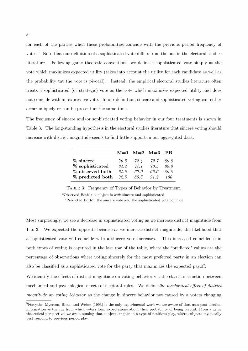
The frequency of sincere and/or sophisticated voting behavior in our four treatments is shown in

Table 3. The long-standing hypothesis in the electoral studies literature that sincere voting should

increase with district magnitude seems to find little support in our aggregated data.

M=1 M=2 M=3 PR

% sincere 70.5 72.4 72.7 89.8% sophisticated 84.2 74.1 70.5 89.8% observed both 64.5 67.0 66.6 89.8% predicted both 72.5 85.5 91.2 100

Table 3. Frequency of Types of Behavior by Treatment.

“Observed Both”: a subject is both sincere and sophisticated.

“Predicted Both”: the sincere vote and the sophisticated vote coincide

Most surprisingly, we see a decrease in sophisticated voting as we increase district magnitude from

1 to 3. We expected the opposite because as we increase district magnitude, the likelihood that

a sophisticated vote will coincide with a sincere vote increases. This increased coincidence in

both types of voting is captured in the last row of the table, where the ‘predicted’ values are the

percentage of observations where voting sincerely for the most preferred party in an election can

also be classified as a sophisticated vote for the party that maximizes the expected payo↵.

We identify the e↵ects of district magnitude on voting behavior via the classic distinction between

mechanical and psychological e↵ects of electoral rules. We define the mechanical e↵ect of district

magnitude on voting behavior as the change in sincere behavior not caused by a voters changing

8Forsythe, Myerson, Rietz, and Weber (1993) is the only experimental work we are aware of that uses past electioninformation as the cue from which voters form expectations about their probability of being pivotal. From a gametheoretical perspective, we are assuming that subjects engage in a type of fictitious play, where subjects myopicallybest respond to previous period play.

9

their strategy but due to the increased likelihood a sophisticated vote is sincere. Instead, the

changes in strategy are coined the psychological e↵ect of district magnitude on voting behavior.

Consider, for instance, a sophisticated voter whose preferred party is the third ranked in number

of votes: when district magnitude is 1 his/her vote is less likely to coincide with his/her sincere

vote than when district magnitude is 2. Note that the strategy of the voter is not changing with

district magnitude yet the way we classify his/her actions is.

Following this distinction, the results in Table 3 suggest that the increase in sincere voting (as we

increase district magnitude) is not driven by a mechanical e↵ect but by a psychological one. This

is possibly due to the higher complexity of computing the correct sophisticated action when district

magnitude is large, which leads voters to be less likely to vote in a sophisticated way and to vote

sincerely instead as district magnitude increases.

Something that seems puzzling in Table 3, though, is the large di↵erence between the percentage

of observations that are both sincere and sophisticated and the situations that are predicted to be

so. It seems that in situations in which both sincere and sophisticated actions coincide, the voter

should have no conflict about supporting his preferred party. However, we observe that around

a 20 percent of subjects fail to choose this action when it is optimal to do so! For whom are

they voting? To our surprise we see that 50 percent of the subjects who did not vote for their

most preferred party (when sincere and sophisticated actions coincide) voted instead for the party

that obtained the most votes in the previous election round. We consequently define this type of

behavior as frontrunner voting: when a subject is voting for the party that obtained the most votes

in the previous period of play.9 Together with this third classification, our three types of behavior

describe more than 90 percent of all vote choices.

Further evidence towards frontrunner behavior is found in our control treatment, with a fully pro-

portional electoral system, where voting sincerely is the dominant strategy. In Figure 1 we depict

the data of our control treatment aggregated by each set of five elections (recall that preferences

are redrawn every five periods) whenever the frontrunner action does not coincide with the sincere

one. That is, we drop observations in which the subject’s preferred party was the most voted party

9Frontrunner voting is only defined for election rounds 2,3,4 and 5 given that in the first election (round 1) preferenceshave been redrawn and there is no previous period of play with the same preferences. In common value situations,voting for the winner can be understood in terms of herding Nageeb and Kartik (2012), information aggregation((Feddersen and Pesendorfer, 1997), or favoring a stable governing party Riambau (2013a). There is no room forsuch rationalizations in our setup.

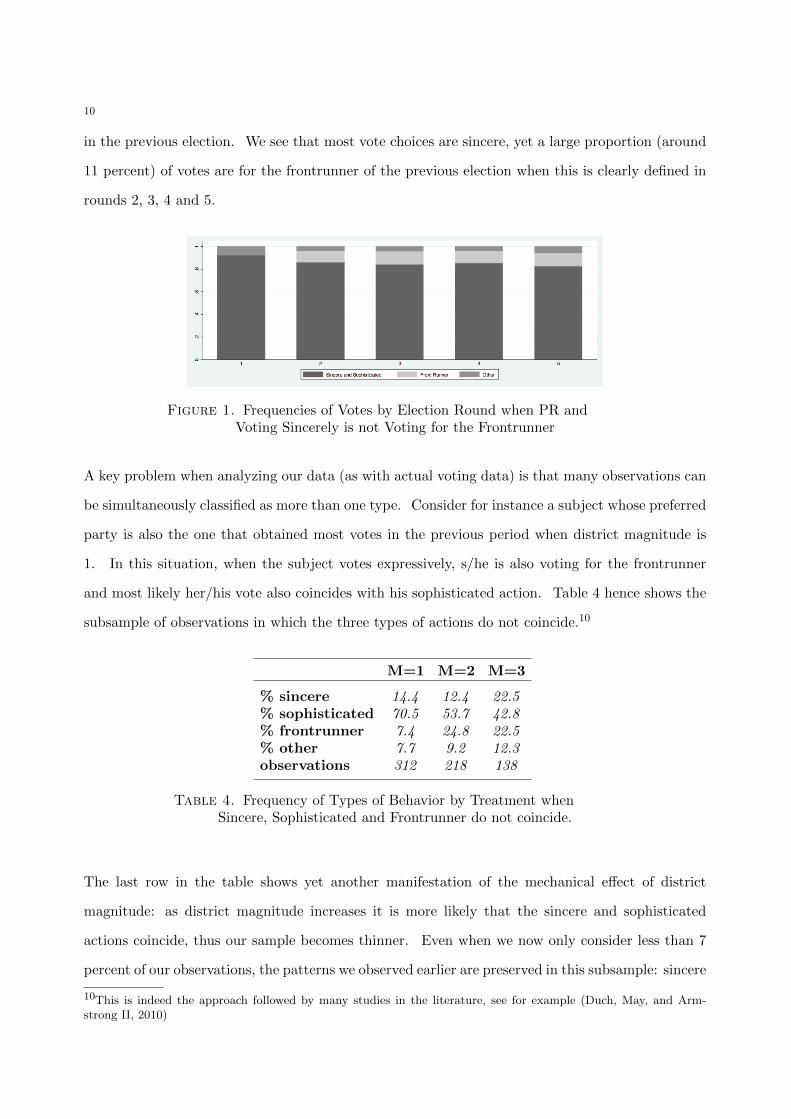
10

in the previous election. We see that most vote choices are sincere, yet a large proportion (around

11 percent) of votes are for the frontrunner of the previous election when this is clearly defined in

rounds 2, 3, 4 and 5.

Figure 1. Frequencies of Votes by Election Round when PR andVoting Sincerely is not Voting for the Frontrunner

A key problem when analyzing our data (as with actual voting data) is that many observations can

be simultaneously classified as more than one type. Consider for instance a subject whose preferred

party is also the one that obtained most votes in the previous period when district magnitude is

1. In this situation, when the subject votes expressively, s/he is also voting for the frontrunner

and most likely her/his vote also coincides with his sophisticated action. Table 4 hence shows the

subsample of observations in which the three types of actions do not coincide.10

M=1 M=2 M=3

% sincere 14.4 12.4 22.5% sophisticated 70.5 53.7 42.8% frontrunner 7.4 24.8 22.5% other 7.7 9.2 12.3observations 312 218 138

Table 4. Frequency of Types of Behavior by Treatment whenSincere, Sophisticated and Frontrunner do not coincide.

The last row in the table shows yet another manifestation of the mechanical e↵ect of district

magnitude: as district magnitude increases it is more likely that the sincere and sophisticated

actions coincide, thus our sample becomes thinner. Even when we now only consider less than 7

percent of our observations, the patterns we observed earlier are preserved in this subsample: sincere

10This is indeed the approach followed by many studies in the literature, see for example (Duch, May, and Arm-strong II, 2010)

11

voting is greater when district magnitude is 3 rather than 1, and sophisticated voting decreases.

Possibly due to the increased complexity of the voting rule we see frontrunner voting and other

behavior increasing with district magnitude.

By construction, the disjoint set never includes the first round of elections when subjects vote just

after preferences have been redrawn. In these cases there is no previous information, so sincere

and sophisticated voting coincides in all treatments. As we discussed above when analyzing our

control treatment, in such elections it is dominant to vote sincerely for the preferred party. Indeed,

we observe a high incidence of such behavior in our data from the very first election – 82 percent of

our first election observations are sincere – and such behavior increases as the experiment unfolds

reaching 90 percent of sincere observations in the first election of the last round of five elections

(election 56).

The patterns we observe are clearly suggestive of both mechanical and psychological e↵ects on

voting behavior in our experiment. The increase in sincere voting is (at least partly) driven by the

mechanical e↵ect of district magnitude. However, if only mechanical e↵ects are present, we should

also be observing an increase in the number of votes that are qualified as sophisticated. Moreover,

frontrunner voting should not increase with district magnitude. Overall, there seems to be a

tendency to move away from sophisticated actions, towards non-rational behavior (as expressed by

sincere and frontrunner voting) as we increase district magnitude. A possible explanation is that as

district magnitude increases it becomes exponentially di�cult to compute the correct sophisticated

action.

Tables 3 and 4 both indicate the heterogeneous e↵ects of district magnitude in our population. If all

subjects were sincere we should observe 100 percent of observations as sincere, while sophisticated

voting should increase with district magnitude due to the mechanical e↵ect, and frontrunner voting

should remain unchanged. Instead, if all subjects were sophisticated, sincere voting should increase

with district magnitude, sophisticated voting should always be at 100 percent, and frontrunner

voting should decrease with district magnitude, because more parties become viable so less voters

need to favor the frontrunner candidate. In the next section we consequently analyze in detail

individual voting decisions, to understand whether district magnitude has a systematic e↵ect on

the heterogeneous behavior of subjects. Our goal, here, is to measure the relative power of the

12

three types of behavior for a representative voter and to see how district magnitude influences the

relative weight of the di↵erent motivations.

4. Individual behavior

Our initial specification assumes that subjects are either sincere or sophisticated: the (unobserved)

indicator function z

soph

it

(zsinit

) takes value 1 if in round t subject i behaves in a sophisticated (sincere)

way, and 0 otherwise. Our goal is to estimate zit

= (zsophit

, z

sin

it

) for all subjects and rounds, i.e. for

each of our treatments we want to identify what is the unconditional probability that a subject is of

each type.11 This unconditional probability can also be interpreted as the proportion of subjects

who are basing their choice solely on their preferences (sincere types), and the proportion who are

also taking into into account their probability of being pivotal (sophisticated types). We will use

both interpretations indistinctly throughout the text.

Let u⇤ijt

be the utility subject i derives from party j in election t; and v

⇤ijt

be the expected utility

i derives from voting for party j in election t. y

ijt

is a dummy variable that takes value 1 when

subject i votes for party j in round t:

y

ijt

= 1 if u⇤ijt

� max(u⇤i1t, u

⇤i2t, ..., u

⇤i5t) and i is sincere)

y

ijt

= 1 if v⇤ijt

� max(v⇤i1t, v

⇤i2t, ..., v

⇤i5t) and i is sophisticated)

y

ijt

= 0 otherwise

where u⇤ijt

= u

j

+↵u

ijt

+"

u

ijt

when z

ssin

it

= 1 and v

⇤ijt

= v

j

+�v

ijt

+"

v

ijt

when z

soph

it

= 1. We assume

"

u

ijt

, "

v

ijt

⇠ type I extreme value. We model the probability that subject i votes for j in period t as

a multinomial logit (MNL):12

p

ijt

(uijt

, v

ijt

; zit

) =e

u

j

+↵u

ijt

P

J

k=1 eu

k

+↵u

ikt

if zsophit

= 0

p

ijt

(uijt

, v

ijt

; zit

) =e

v

j

+�v

ijt

P

J

k=1 ev

k

+�v

ikt

if zsophit

= 1

11Note that in this first specification we have that zsophit

= 1� zsinit

.12The reported results impose that the constants u

j

and vj

are equal 8j. That is, the mean propensity of voting foreach party is the same regardless of the type (we find analogous results when we relax this condition).

13

Note that modeling utilities with a MNL allows us to take into account cardinality of preferences:

the likelihood of voting for one party depends not only on the ranking of the party in an ordinal

setting, but on the cardinal utility this party yields relative to all other parties.

Given that the type z = (zsin, zsoph) is unobserved, we can at most infer the probability that

each subject is of each type. We estimate z’s using the Expectation-Maximization algorithm.13

Arcidiacono, Sieg, and Sloan (2007) elegantly summarizes what we do: given initial values of

the parameters, we first calculate the conditional probability that an individual is a particular

type; using these conditional probabilities as weights, we treat types as observed and we maximize

the (now) additively separable log-likelihood function; given the new parameter estimates, we

then update the conditional probabilities of being each of the types and iterate until convergence

(Arcidiacono, Sieg, and Sloan, 2007).14 Since the likelihood of being a particular type is always

strictly positive, we find that even when a vote seems to unambiguously be of type z, the algorithm

can only assign it a probability of being of type z which is arbitrarily close to 1, but never 1 (and,

in some cases, given the available information, even not necessarily close to one). In the Appendix

we specify all computational details of the EM algorithm.

Throughout, we do a double exercise. First, we pool all observations for each district magnitude,

and run the EM algorithm just once per district magnitude – i.e. we run it four times (M=0,1,2,3).

For each action we find z

it

and report the average across all individuals and periods (panels A in

tables below). In other words, we first assume that all observations are independent. Second,

given that for each subject we have many observations, we run the algorithm once per subject.15

In this case we also report the averages across all subjects (panels B in tables below). This second

set of regressions can be interpreted as controlling for individual fixed e↵ects given that we are

estimating z’s for each subject separately. We can advance that results di↵er slightly among our

two types of regressions but the patterns are the same regardless of which specification we use.

Table 5 reports the results for the two types model. For each district magnitude we report the

percentage of individuals classified as sincere and those who are classified as sophisticated. We

13See Dempster, Laird, and Rubin (1977) and Fruhwirth-Schnatter (2006) for detailed descriptions of the algorithm.14Our strategy is similar to that of Duch, May, and Armstrong II (2010): in both cases types are unobserved and fromthe data we can at most infer the probability that each subject is of each type at each round. Nevertheless, whereasDuch, May, and Armstrong II (2010) use Bayesian methods, we use the computationally simpler EM algorithm, asin Riambau (2013b).15Given that we do not include first round observations when sophisticated and sincere coincides we have 48 obser-vations per subject.

14

also report the percent of correct vote predictions using z

it

and the parameters of the model. In

both panels A and B the estimated proportion of sincere types sharply increases with district

magnitude. This is a strong result, yet we have to remember that for a large proportion of our

observations, sincere and sophisticated actions are observationally equivalent. This means that we

are forcing our algorithm to decide between two types when both are potentially correct. Note that

there are no results for our fully proportionality treatment because in these cases both sincere and

sophisticated behavior are equivalent. Note also that the percentage of observations we correctly

classify decreases with district magnitude but always reaches a high score.

M=1 M=2 M=3

Panel A: Whole sample

% sincere 21.98 33.49 55.99% sophisticated 78.02 66.51 44.01

% correct 87.24 76.79 68.60observations 2,304 2,400 3,360

Panel B: Average across subjects

% sincere 30.56 36.24 51.50% sophisticated 69.44 63.76 48.50

% correct 92.07 81.30 76.29observations 2,256 2,352 3,312

Table 5. Proportion of subjects of each type (2 types)

We check statistical significance on the increase in the proportion of sincere voters by running a

Kolmogorov-Smirnov test: for each district magnitude, the null hypothesis is that the cumulative

distribution function of the distribution of zsinijt

s for M + 1 is not larger than the same one for

M . We do not report the results but we find this hypothesis rejected in both cases. That is, the

distribution of zsinit

s increase with district magnitude.16

Following our previous discussion, we next introduce a third type that captures whether subjects

vote for the frontrunner party in the previous election. We denote it z

FR = 1 � z

sin � z

soph.

Formally, for this type y

ijt

is equal to 1 if in the previous round party j obtained the most votes,

16Note that panel B has slightly less observations than panel A. This is because in each treatment we had to dropone subject to reach convergence in our algorithm.

15

and is equal to 0 otherwise. The utility of this type of voter is given by:

p

ijt

(uijt

, v

ijt

, FR

ijt

; zit

) =e

�

j

+↵FR

ijt

P

J

k=1 e�

k

+↵FR

ikt

if zFR

it

= 1

where FR

j

is a dummy that takes value 1 if j was the party with most votes in the previous round

and 0 otherwise.

Table 6 shows the results for the three types model. We consistently find the same patterns: in

both panels A and B, the proportion of sincere actions increases with district magnitude. This

result is statistically significant when using the Kolmogorov-Smirnov test. Interestingly, it is worth

noting that around one in every ten votes is classified as frontrunner. This is indeed the proportion

we observed in our control treatment with a fully proportional electoral system.

M=1 M=2 M=3 PR

Panel A: Whole sample % sincere

% sincere 19.99 20.41 35.86 85.91% sophisticated 71.04 63.73 53.89% frontrunner 8.97 15.86 10.25 14.09

% correct 91.32 79.58 78.24 91.10observations 2,304 2,400 3,360 2,112

Panel B: Average across subjects % sincere

% sincere 27.30 29.41 41.62 86.95% sophisticated 63.67 55.82 38.50% frontrunner 9.03 14.77 19.88 13.05

% correct 95.30 87.07 85.45 94.41observations 2,256 2,352 3,312 2,112

Table 6. Proportion of subjects of each type (3 types)

As was noted in Section 3, one of the main issues with our experimental design is that many

actions are observationally equivalent. As a robustness check we now look at the subsample of

observations in which the three types of action do not coincide. Note that there is no self-selection

into this subsample: utilities are randomly assigned every five elections. Besides, expected utilities

are computed given the behavior of all subjects in the previous round so there is no way a subject

can choose a particular ordering of parties according to utilities or expected utilities. The median

number of observations per individual is 16, 9 and 5 in the treatments with district magnitude 1, 2,

and 3, respectively. This once again captures the mechanical e↵ect of district magnitude. Table 7

16

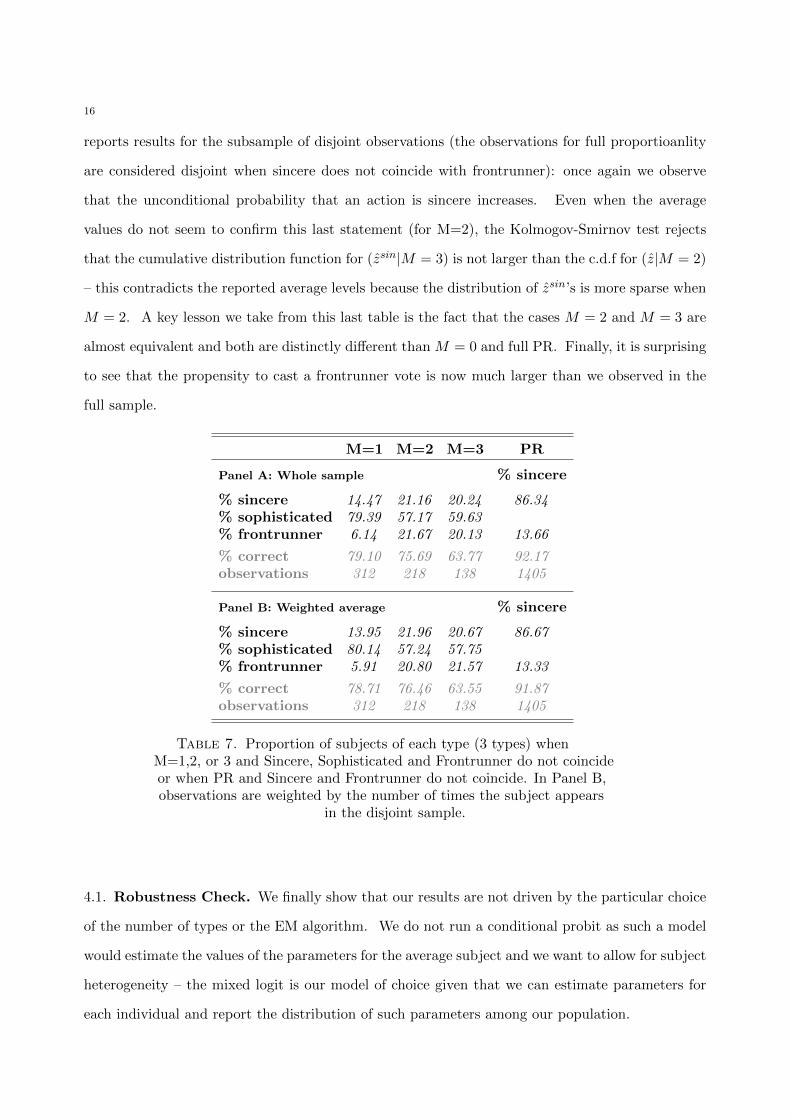
reports results for the subsample of disjoint observations (the observations for full proportioanlity

are considered disjoint when sincere does not coincide with frontrunner): once again we observe

that the unconditional probability that an action is sincere increases. Even when the average

values do not seem to confirm this last statement (for M=2), the Kolmogov-Smirnov test rejects

that the cumulative distribution function for (zsin|M = 3) is not larger than the c.d.f for (z|M = 2)

– this contradicts the reported average levels because the distribution of zsin’s is more sparse when

M = 2. A key lesson we take from this last table is the fact that the cases M = 2 and M = 3 are

almost equivalent and both are distinctly di↵erent than M = 0 and full PR. Finally, it is surprising

to see that the propensity to cast a frontrunner vote is now much larger than we observed in the

full sample.

M=1 M=2 M=3 PR

Panel A: Whole sample % sincere

% sincere 14.47 21.16 20.24 86.34% sophisticated 79.39 57.17 59.63% frontrunner 6.14 21.67 20.13 13.66

% correct 79.10 75.69 63.77 92.17observations 312 218 138 1405

Panel B: Weighted average % sincere

% sincere 13.95 21.96 20.67 86.67% sophisticated 80.14 57.24 57.75% frontrunner 5.91 20.80 21.57 13.33

% correct 78.71 76.46 63.55 91.87observations 312 218 138 1405

Table 7. Proportion of subjects of each type (3 types) whenM=1,2, or 3 and Sincere, Sophisticated and Frontrunner do not coincideor when PR and Sincere and Frontrunner do not coincide. In Panel B,observations are weighted by the number of times the subject appears

in the disjoint sample.

4.1. Robustness Check. We finally show that our results are not driven by the particular choice

of the number of types or the EM algorithm. We do not run a conditional probit as such a model

would estimate the values of the parameters for the average subject and we want to allow for subject

heterogeneity – the mixed logit is our model of choice given that we can estimate parameters for

each individual and report the distribution of such parameters among our population.

17

In our approach we have implicitly assumed that the value of each of our parameters is the same

within each type and we have then assigned each of our subjects a probability of being each

type (z’s). Instead, the mixed logit assumes that all subjects simultaneously take into account

utilitarian, sophisticated and frontrunner considerations (and allows subjects to place di↵erent

weight on each component). Formally we have that:

p

ijt

(uijt

, v

ijt

, FR

ijt

) =e

↵

j

+�

i

sin

u

ijt

+�

i

soph

v

ijt

+�

i

FR

FR

ijt

P

J

k=1 e↵

k

+�

i

sin

u

ikt

+�

i

soph

v

ikt

+�

i

FR

FR

ikt

where0

B

B

B

B

@

�

i

sin

�

i

soph

�

i

FR

1

C

C

C

C

A

⇠ N

0

B

B

B

B

B

B

B

@

�

sin

�

2sin

�

sinsoph

�

sinFR

�

soph

, �

sinsoph

�

2soph

�

sophFR

�

FR

�

sinFR

�

sophFR

�

2FR

1

C

C

C

C

C

C

C

A

We assume that the distribution of the vector of parameters � follows a multivariate normal distri-

bution. Below we report the estimated means of our mixed logit computations (covariance matrices

are available upon request).

M=1 M=2 M=3 PR

Mean �

sin

2.97 1.92 3.78 14.99(0.50) (0.26) (0.32) (1.20)

Mean �

soph

90.84 80.24 63.61(9.57) (6.14) (6.68)

Mean �

FR

1.66 0.77 1.02 1.98(0.15) (0.12) (0.11) (0.88)

% correct 78.26 70.75 66.90 85.23observations 2,304 2,400 3,360 2,112

Table 8. Mixed Logit Results

(standard errors in brackets)

Note that the scale of the utility and expected utility values are not the same so parameters in our

four di↵erent specifications are not directly comparable. However, we can observe similar trends

as those we observed earlier: sincere considerations (as captured by �

sin

) increase with district

magnitude in all cases apart from M = 1 to M = 2; sophisticated considerations (as captured

18

by �

soph

) decrease with district magnitude in all cases; and finally, frontrunner considerations are

always present. In terms of the percentage of correct observations we see that our EM algorithm

has a much greater predictive power than the mixed logit model. Duch, May, and Armstrong II

(2010) run a similar comparison with the mixed logit model and define the Proportional Reduction

in Error (PRE) as:

PRE =#{correct types model}�#{correct mixed logit }

N �#{correct mixed logit}

where N is the total number of observations. We can compute this score for each of our treatments

and we find that the relative improvement of the EM algorithm with respect to the more standard

mixed logit is always above 30 percent and reaches its maximum for the M=1 treatment in which

PRE is 60.1 percent.17

5. Conclusions

A widely-held assumption in political science is that non-sincere voting should be lower in higher-

magnitude districts. Yet, formal work on the probability of being pivotal as well as actual voting

data from elections suggests that voters are just as sophisticated in multi-member districts are they

are in single-member districts. One problem for empirical research, however, is that it is almost

impossible to isolate the e↵ect of district magnitude on voting behavior independently of voters’

preferences or parties’ positions. We hence designed a lab experiment to isolate this e↵ect, by

varying district magnitude while keeping voters’ preferences and parties’ positions constant.

We do find a decrease in sophisticated voting as district magnitude increases. But, we also find

evidence of a mechanical e↵ect of district magnitude on the propensity to vote sincerely for a voter’s

most preferred party. As district magnitude increased, the proportion of voters who found that

their most preferred party would also now yield them the highest expected utility (and hence that

their sincere and sophisticated motivations coincided) also increased. Nevertheless, not as many

participants voted for their most preferred party when their sincere and sophisticated motivations

coincided as we expected.

We also found that sophisticated voting does not increase with district magnitude and that there

was a high incidence of voting for the winner of the previous election (the frontrunner) in all our

17PRE values are 60.1%, 30.2%, 34.3% and 39.7% for DM=1,2,3 and PR, respectively.

19

treatments (we even find the latter to be the case in our control with fully proportional elections -

above 10 percent of such observations). Following our classification of mechanical and psychological

e↵ects, we have indeed seen that as we increase district magnitude we find that there is an increase in

sincere voting possibly due to a mechanical e↵ect. However, our results suggest that the decrease in

sophisticated voting and the increase in frontrunner voting can only be classified as a psychological

e↵ect of the increase in district magnitude, possibly due to the rising complexity of calculating the

’correct’ sophisticated action.

This last aspect, the presence of frontrunner voting, has not received much attention in the empirical

and theoretical studies of voting. However, as Hinich (1981) points out: ”voting for the winner is

no less plausible than the assumption that voters believe they can be pivotal”.

References

Abramson, P. R., J. H. Aldrich, A. Blais, M. Diamond, A. Diskin, I. H. Indridason,

D. J. Lee, and R. Levine (2010): “Comparing Strategic Voting Under FPTP and PR,” Com-

parative Political Studies, 1(43), 61–90.

Arcidiacono, P., H. Sieg, and F. Sloan (2007): “Living Rationally Under the Volcano? An

Empirical Analysis of Heavy Drinking and Smoking,” International Economic Review, 48(1),

37–65.

Austen-Smith, D., and J. S. Banks (1988): “Elections, Coalitions and Legislative OutcomeS,”

American Political Science Review, 2(82), 405–422.

(1996): “Information Aggregation, Rationality and the Condorcet Jury Theorem,” Amer-

ican Political Science Review, 1(90), 35–45.

Bargstad, M. A., and O. Kedar (2009): “Coalition-Targeted Duvergerian Voting: How Expec-

tations A↵ect Voter Choice under Proportional Representation,” American Journal of Political

Science, 2(53), 307–323.

Blais, A., J. Aldrich, I. Indridason, and R. Levine (2006): “Do Voters Vote for Government

Coalitions? Testing Downs’ Pessimistic Conclusion,” Party Politics, 6(12), 691–705.

Borman, S. (2009): “The Expectation Maximization Algorithm A short tutorial,” mimeo.

Callander, S. (2008): “Majority Rule when Voters like to Win,” Games and Economic Be-

haviour, 2(64), 393–420.

20

Carey, J., and S. Hix (2011): “The Electoral Sweet Spot: Low-Magnitude Proportional Electoral

Systems,” American Journal of Political Science, 2(55), 383–339.

Cox, G. W. (1994): “Strategic Voting Equilibria Under the Single Nontransferable Vote,” Amer-

ican Political Science Review, 3(88).

(2007): Making Votes Count: Strategic Coordination in the World’s Electoral Systems.

Cambridge University Press, Cambridge.

Dempster, A., N. M. Laird, and D. B. Rubin (1977): “Maximum Likelihood from Incomplete

Data via the EM Algorithm,” Journal of Royal Statistical Society, Series B (Methodological),

1(39), 1–38.

Duch, R., J. May, and D. A. Armstrong II (2010): “Coalition-directed Voting in Multiparty

Democracies,” American Political Science Review, 104, 698–719.

Duverger, M. (1954): Political Parties: Their Organization and Activity in the Modern State.

John Wiley, New York, NY.

Feddersen, T. J., and W. Pesendorfer (1996): “The Swing Voter’s Curse,” American Eco-

nomic Review, 3(86), 408–424.

(1997): “Voting Behavior and Information Aggregation in Elections With Private Infor-

mation,” Econometrica, 5(65), 1029–1058.

Feddersen, T. J., and A. Sandroni (2006): “A Theory of Participation in Elections,” American

Economic Review, 4(96), 1271–1282.

Fey, M. (1997): “Stability and Coordination in Duverger s Law: A Formal Model of Preelection

Polls and Strategic Voting,” American Political Science Review, 1(91), 135–147.

Fischbacher, U. (2007): “Z-Tree: Zurich Toolbox for Ready-Made Economic Experiments,”

Experimental Economics, 2(10), 171–178.

Fischer, A. J. (1996): “A Further Experimental Study of Expressive Voting,” Public Choice,

1(88), 171–180.

Forsythe, R., R. B. Myerson, T. A. Rietz, and R. J. Weber (1993): “An Experiment

on Coordination in Multi-candidate Elections: The Importance of Polls and Election Histories,”

Social Choice and Welfare, 3(10), 223–247.

Fruhwirth-Schnatter, S. (2006): Finite Mixture and Markov Switching Models. Springer Series

in Statistics, New York.

21

Gerber, E. R., R. B. Morton, and T. A. Rietz (1998): “Minority Representation in Multi-

Member Districts,” American Political Science Review, 1(92), 127–144.

Greiner, B. (2004): “The Online Recruitment System ORSEE 2.0: A Guide for the Organization

of Experiments in Economics,” Working Paper Series in Economics - University of Cologne, 10.

Hinich, M. J. (1981): “Voting as an Act of Contribution,” International Economic Review, 36(1),

135–140.

McCuen, B., and R. B. Morton (2006): “Tactical Coalition Voting and Information in the

Laboratory,” Electoral Studies, 3(29), 316–328.

Morton, R., D. Muller, L. Page, and B. Torgler (2013): “Exit Polls, Turnout, and Band-

wagon Voting: Evidence from a Natural Experiment,” mimeo.

Myerson, R. B., and R. J. Weber (1993): “A Theory of Voting Equilibria,” American Political

Science Review, 1(87), 102–114.

Nageeb, A., and N. Kartik (2012): “Herding with Collective Preferences,” Economic Theory,

51, 601–626.

Piketty, T. (2000): “Voting as Communicating,” Review of Economic Studies, 1(67), 169–191.

Reynolds, A., and M. Steenbergen (2006): “The Political Consequences of Ballot Design,

Innovation and Manipulation,” Electoral Studies, 3(25), 570–598.

Riambau, G. (2013a): “Bandwagon in Israel? Note on Bargsted and Kedar (2009),” mimeo.

(2013b): “Voting for Parties or Policies? Evidence from Israel,” mimeo.

Sartori, G. (1968): Political Development and Political Engineering. Cambridge University Press,

New York, NY.

22

6. Appendix

6.1. Instructions. (treatment M=2)Thank you for agreeing to participate in our voting experiment. The sum of money you will earn duringthe session will be given privately to you at the end of the experiment. From now on (and until the end ofthe experiment) you cannot talk to any other participant. If you have a question, please raise your handand one of the instructors will answer your questions privately. Please do not ask anything aloud! Youbelong to a group of 25 participants with whom you will interact for 60 elections. The rules are the samefor all participants and for all elections. In each election the group will vote to elect two candidates. Thewinning candidates will be selected by a form of proportional representation, where each party will win seatsin proportion to their share of the vote. After each election you will be announced the outcome and your“profit” in such election. At the end of the experiment you’ll be asked to answer a questionnaire.

6.1.1. Voting procedure. The party with the most votes wins the first seat, and its vote-total is then dividedby 3. The party with the highest remaining votes wins the second seat. In the case of a tie, the winner isdetermined randomly. As an illustration consider the following example:

Party A B C D EVotes 2 9 2 7 5Votes÷ 3

As a result, parties B and D each obtain a candidate because 9 and 7 are the highest numbers. Now considera di↵erent example where parties obtain the following number of votes:

Party A B C D EVotes 15 1 4 2 3Votes÷ 5

In this second example, Party A obtains 2 candidates because 15 and 5 are the highest numbers.

6.1.2. Profits in each election. The profits you receive in each election depend on the candidates elected bythe group regardless of whether you voted for any of them. Your profit will be equal to the sum of yourvaluation of the party of each elected candidate. The table below shows five hypothetical valuations for eachof the five parties:

Party A B C D EYour valuations 500 1200 100 1800 500

So, if the 2 candidates from party A are elected, you obtain a profit of 1000 ( = 500 + 500). Alternatively,if one candidate from party C is elected, and one candidate from party D is elected you obtain a profit of1900 (= 100 + 1800). It is important to note that (a) your valuations are di↵erent from the valuations ofall other voters; and (b) that no other voter knows the valuations of any other voter.

6.1.3. Final Payment. At the end of the last election, the computer will randomly select 4 elections and youwill earn the sum of the profits on those elections in pennies. Additionally you will be paid three pounds fortaking part in the experiment.

6.1.4. Questionnaire. (prior to the beginning of the session)1. When the winners of an election are known, do you know your profit in such election? YES/NO2. When the winners of an election are known, do you know the profit of any other participant? YES/NO3. Imagine that party A obtains more votes than party B. Could it ever be the case that party B obtainsmore candidates than party A? YES/NO4. Imagine a situation where the votes obtained by each party are given by the table below. What wouldthe outcome of the election be?

Party A B C D EVotes 15 2 1 7 0

• Two candidates from party A• One candidate from party D and one from party E• One candidate from party A and one from party D• Two candidates from party B

23

5. Consider a situation where your valuations and the votes obtained by each party are given by the tablebelow. Imagine you voted for party B, what would your profit be?

Party A B C D EVotes 15 2 1 7 0

Your Valuations 500 1200 100 1800 500

• 1000 or 1200 or 2400 or 0 or 2300

6. Who is going to be paid at the end of the experiment?

• No one• 1 person according to his/her profit in various elections• 2 people according to their profit in various election• Everyone according to his or her profit in four elections• Everyone according to his or her average profit throughout the experiment

!

!Screenshot!at!the!beginning!of!election!1!

!

!Screenshot!after!election!1!

!

!Screenshot!at!the!beginning!of!election!2!

!

Figure 2. Screenshots of the Ztree program for the treatment M=2.

24

6.2. Location of Political Parties. In all our sessions, the location of the parties and the voters werere-drawn after each set of five elections. We alternated between two types of party locations, shown in theFigure below. So, elections 1 to 5, 11 to 15, 21 to 25, 31 to 35, 41 to 45, and 51 to 55 where held with theType A locations of the parties. And, elections 6 to 10, 16 to 20, 26 to 30, 36 to 40, 46 to 50, and 56 to 60where held with the Type B locations of the parties. Note that in the Type B elections we assumed radialsymmetry so that there were many more players that were indi↵erent between various parties. The labellingof parties (from A to E) was randomly allocated in each set of five elections. Given that the participantswere not aware of the two-dimensional location of their preferences and the relative location of the parties,when we switched between the two types of party locations we simply announced that the preferences hadbeen redrawn. We clearly stated that the next five elections were independent from the previous five.

020

4060

80100

0 20 40 60 80 100

020

4060

80100

0 20 40 60 80 100

Figure 3. Location of political parties. In all treatments, subjects’ preferred policiesare uniformly distributed in the two dimensional policy space [0, 100]⇥ [0, 100].

6.3. Sophisticated voting. A subject’s sophisticated vote takes into account not only his or her utility butalso the probability his or her vote will be pivotal. The latter component depends on the subject’s beliefsabout the distribution of votes. Using the theory of voting equilibria Myerson and Weber (1993) we willassume that any subject assumes that the probability that any other subject votes for party k is equal to thevote share obtained by each party in the previous round of election. That is, p

k

= vkvA+vB+vC+vD+vE

, where

(vA

, v

B

, v

C

, v

D

, v

E

) are the votes received by each of the five parties in the previous round of elections.18

Knowing these probabilities, we can compute the probability that party A gets a votes, candidate B gets bvotes, and so on, out of n-1 voters using the following multinomial probability:

f(a, b, c, d, e) =(n� 1)!

a!b!c!d!e!· pa

A

· pbB

· pcC

· pdD

· peE

where a + b + c + d + e = n � 1. Given a distribution of votes in the previous election, there is then afunction that assigns seats to each of the five parties (taking into account the district magnitude and theseat allocation formula, in our case Sainte-Lague for the M=2 and M=3 treatments). We denote the seatsassigned to party k given a particular vote distribution as ⌦

k

(a, b, c, d, e). The expected utility of a subjectwith preferences I when voting for party A can then be expressed as follows:

E (u✓

(vote for party A) =X

(a,b,c,d,e)2V

0

@

X

k=A,B,C,D,E

⌦k

(a+ 1, b, c, d, e) · ✓k

· f(a, b, c, d, e)

1

A

where ✓ is the type of the voter (the utility he assign to each party) and V is any possible combination ofvotes for the five parties so that they add up to (n-1).

In our experimental setting, we restrict our attention to situations in which being sophisticated is solelydriven by the probability of being pivotal. There are, however, many motivations that may lead voters tovote non sincerely in real elections. Voters may use their votes to communicate their preferences (Piketty,2000). They may anticipate the best candidate to be elected given other citizens’ votes (Austen-Smith andBanks, 1996; Feddersen and Pesendorfer, 1996, 1997). Or, they may try to influence the coalition formationin the legislature (Austen-Smith and Banks, 1988; Blais, Aldrich, Indridason, and Levine, 2006; Bargstadand Kedar, 2009; Duch, May, and Armstrong II, 2010; McCuen and Morton, 2006).

18In the first round of elections, just after preferences have been redrawn, there is no previous round on which tocondition the voting decision so the sophisticated vote coincides with the sincere one: voting for most preferred party.

25

6.4. Estimation Procedure. Suppose we want to find ✓ which maximizes P (X|✓), ✓ = (↵,�,⇡). Say thatwe have an unobserved random variable Z, with a given realization z (WLOG, for simplicity let us assumethat z = z

soph, and that ⇡ is the unconditional probability that an action is of type ‘sophisticated’. Also forsimplicity we will omit subscript ‘t’). Then

✓0 ⌘ argmax✓

logP (X|✓) = argmax✓

log

(

X

z

P (X|z, ✓)P (z|✓))

(1)

In Borman (2009) it is shown that

max✓

log

(

X

z

P (X|z, ✓)P (z|✓))

� max✓

X

z

P (z|X, ✓

⌧

) log P (X, z|✓) (2)

where ✓⌧

is the set of estimated parameters at iteration t. That is, given a set of estimates ✓⌧

,P

z

P (z|X, ✓

⌧

) log P (X, z|✓)is bounded above by logP (X|✓). Therefore, given an unobserved vector z and an educated initial guess ✓0,maximizing the RHS of (2) will yield us ✓, the best approximation to ✓0.Since in our case

P

i

(Xi

|zi

, ✓) =⇣

f

soph

i

⌘

zi �

f

pty

i

�(1�zi)

P

i

(zi

|✓) = ⇡

P

i

(zi

|Xi

, ✓

⌧

) = z

i

(Xi

,↵

⌧

,�

⌧

,⇡

⌧

) and

P

i

(Xi

, z

i

|✓) =⇣

⇡f

soph

i

⌘

zi �

(1� ⇡)fsin

i

�(1�zi)

we have that the best approximation to

argmax↵,�,⇡

logLIK(X|z,↵,�,⇡) =N

X

i

log

n

⇡

⇣

f

soph

i

⌘

zi

+ (1� ⇡)�

f

sin

i

�(1�zi)o

is given by

argmax↵,�,⇡

N

X

i=1

z

i

(.)log⇣

⇡f

soph

i

⌘

+ (1� z

i

(.))log�

(1� ⇡)fsin

i

�

=

argmax↵,�,⇡

N

X

i=1

z

i

(.)log (⇡) + z

i

(.)log⇣

f

soph

i

⌘

+ (1� z

i

(.))log (1� ⇡) + (1� z

i

(.))log�

f

sin

i

�

which is what one actually maximizes.

6.5. The M-STEP in detail. We will omit subscript ⌧ for ease of notation. At iteration ⌧ , in order to getestimates of {↵,�,⇡}, we need to solve

argmax↵,�,⇡

N

X

i=1

{zi

log⇡ + (1� z

i

)log(1� ⇡)}+N

X

i=1

z

i

8

<

:

X

j

y

ij

log(Pij

|zi

= 1)

9

=

;

+N

X

i=1

(1� z

i

)

8

<

:

X

j

y

i1log(Pij

|zi

= 0)

9

=

;

(3)

Recall that

(Pij

|zi

= 0) =e

uij↵+�j

P

J

j=1 euij↵+�j

(Pij

|zi

= 1) =e

vij�+�j

P

J

j=1 evij�+�j

�

j

= [�1, �2, ..., �5] with �1 = [0, 0, 0, 0, 0] for the base outcome

and 1yij = 1 if i votes for j, 0 otherwise.

(4)

26

FOCs yield:

[⇡] ) ⇡ =

P

N

i

z

i

N

[↵] ) @logLIK@↵

=N

X

i

1yij ⇥ z

i

⇥ ( ij

|zi

= 1)⇥ v

ij

+

N

X

i

1yij ⇥ (1� z

i

)⇥ ( ij

|zi

= 0)⇥ u

ij

=! 0

[�s,j

] ) @logLIK@�

s,j

= �N

X

i

1yij ⇥ z

i

⇥ (Pij

|zi

= 1)⇥ x

a

i

�

N

X

i

1yij ⇥ (1� z

i

)⇥ (Pij

|zi

= 0)⇥ x

a

i

=! 0

where

( ij

|zi

= 1) =

P

j

e

vij↵+�j ⇥ v

ij

P

j

e

vij↵+�j, �

j

= [0, 0, ..., 0] for the base outcome

( ij

|zi

= 0) =

P

j

e

uij↵+�j ⇥ u

ij

P

j

e

uij↵+�j,

Note: Since the likelihood conditional on any type is always strictly positive, then we find that even when avote is obviously sincere, the algorithm can only assign it a probability of being sincere which is arbitrarilyclose to one, but never one (and, in some cases, given the available information, is not necessarily close toone). Moreover, the probability assigned to each single action depends not only on all the information wehave on that action (embedded in the likelihood function), but also on the average of all the probabilitiesassigned to all actions in the previous round. Therefore, even if in one particular round a voter cast a votethat was unambiguously sincere, it is likely that the probability assigned by the algorithm converges to butis not one. for each action, the probability that it is of type z is a weighted average of the likelihoodsconditional on that action being of all possible types (sincere, sophisticate, frontrunner). More specifically,these probabilities are defined at each iteration r as follows by the EM algorithm :

Pr(action ait

=type z) in iteration r ⌘

z

it

(r) =⇧

z

· Likelihood ait

| ait

=type z

⇧sin

· (Lik. ait

| ait

=sin) +⇧sin

· (Lik. ait

| ait

=soph.) +⇧FR

· (Lik. ait

| ait

=FR)

z = {sincere, sophisticated, frontrunner}

⇧z

=N

X

i

T

X

t

z

it

(r � 1)

(5)