the dynamics of retail oligopoly - paul.ellicksonpaulellickson.com/smdynamics.pdf · the dynamics...

The Dynamics of Retail Oligopoly

Arie Beresteanu�

Duke UniversityPaul B. Ellicksony

University of RochesterSanjog Misra

University of Rochester

April, 2010

AbstractThis paper examines competition between supermarkets as a dynamic discrete game

between heterogeneous players. We focus on the impact of Wal-Mart�s entry on incum-bent supermarket �rms, quantifying the impact on welfare and competition. Employinga unique thirteen year panel dataset of store level observations that includes every super-market �rm operating in the United States alongside the rapid proliferation of Wal-Martsupercenters, we propose and estimate a dynamic structural model of chain level com-petition in which incumbent �rms choose each period whether to add or subtract storesor exit the market entirely, and potential entrants choose whether or not to enter. Prod-uct market competition is modeled as Nash in prices, incorporating detailed informationon prices and characteristics and unobserved heterogeneity in chain-level quality. Ourestimation approach combines two-step estimation methods with a one-period ahead(renewal) representation of the value function. This structure serves several purposes.First, it allows us to accommodate a continuous state space, which is essential giventhe wide range of markets in which supermarket �rms compete. Second, it allows fora certain form of incompleteness in the sampling scheme, stemming from the fact thatWal-Mart has yet to exit a market or close a supercenter. Finally, it allows us to includestructural errors for all actions, including investment. Using the results from the struc-tural estimation, counterfactuals quantifying the welfare impact of Wal-Mart�s entry areperformed using an extension of the Pakes and McGuire (2001) stochastic algorithm.

�The authors would like to thank seminar participants at Cornell, Duke, Harvard, Northwestern, PennState, the Federal Reserve, the Federal Trade Commision, the Department of Justice and the AEA wintermeetings. Any remaining errors and omissions are our own.

yCorresponding author: Paul B. Ellickson ([email protected])

1

1 Introduction

Retail �rms account for a surprising fraction of economic activity. In particular, retailers

employ over 20% of the private sector workforce and produce nearly 13% of US GDP.

Furthermore, mass merchandisers like Wal-Mart and Target have led the way in developing

and di¤using innovative information technologies, often forcing upstream producers to lower

prices and make complementary cost reducing investments. The rise of the �big box�format

and a continued emphasis on one stop shopping has both increased the variety of products

and lowered their costs. At the same time, many retail industries have become highly

concentrated. Most �category killers�now compete locally with only one or two rivals. In

some categories, like o¢ ce supplies, there are only two or three chains nationwide. Viewed

more broadly, these industries exhibit a highly skewed size distribution: a few giant chains

compete with a large number of small local players. While the explosion in variety and

reduction in price is unambiguously bene�cial to consumers, the increase in concentration

may be cause for concern. Fear of increased in concentration and impact on small businesses

has triggered many municipalities to pass zoning laws restricting entry of �big-box�stores

to their markets. The goal of this paper is to develop a model of retail chain competition

in which the impact of restrictions on competition between retail chains on competition,

prices and consumer and total welfare can be evaluated.

The theoretical framework proposed in this paper is based on the Markov perfect equi-

librium (MPE) framework of Ericson and Pakes (1995), in which �rms make competitive

investments that increase the quality of their products. In the context of retail competition,

in which �rms operate a chain of individual stores, quality is a function of the total number

of stores operated by each �rm, the individual characteristics of their stores, and their over-

all format (conventional supermarket or Supercenter). Allowing �rms to adjust all of these

features independently would yield an intractably complex control problem. Instead, our

strategy is to focus on a single dimension of quality (store density) and allow �rms to di¤er

by format (supermarket or Supercenter). Product market competition is modeled using a

discrete choice model of demand, in which �rms may also di¤er by a measure of �perceived�

quality that is �xed over time. We assume that the economically relevant features of the

industry can be encoded into a state vector that includes each �rm�s store density, its over-

2

all format, and its perceived level of quality. Firms receive state dependent payo¤s in the

product market and in�uence the evolution of the state vector through their entry, exit,

and investment decisions. In particular, �rms can adjust their chain size each period by

either opening new stores or closing existing ones. Equilibrium occurs when �rms choose

strategies that maximize their expected discounted pro�ts, given the expected actions of

their rivals.

We estimate this model of competition using a unique panel dataset that follows the en-

tire supermarket industry over thirteen consecutive periods (years). Our estimator is based

on the two-step procedure proposed by Aguirregabiria and Mira (2007), using an alternative

representation of the value function suggested by Arcidiacono and Miller (2008). In the �rst

step, we recover the �rm�s policy functions governing entry, exit, and investment. These

functions characterize �rms beliefs regarding the evolution of the common state variables

and the actions of their competitors. We also estimate the per-period payo¤ that each �rm

receives as a function of the current state. In the second step, we use the structure of the

MPE to recover the parameters that make those beliefs optimal. Following Hotz and Miller

(1993), this is accomplished by replacing the continuation values in the best response proba-

bility functions with inverted conditional choice probabilities (CCPs) that can be recovered

non-parametrically from the data. To accommodate our large state space and rich choice

set, we use Monte Carlo simulation to construct these �nuisance�parameters, and estimate

the structural parameters using simulated pseudo maximum likelihood. Having recovered

the structural parameters of the underlying model, we then perform policy experiments

aimed at evaluating the impact of zoning laws that prevent the growth of Supercenters on

investment, market structure, and consumer and producer surplus, using a discrete control

version of the Pakes and McGuire (2001) stochastic algorithm.

This paper builds on both the sizable empirical literature on static entry games as well

as more recent work on dynamic games. Until recently, the empirical entry literature has

mainly employed static models of competition. As a consequence, the early papers were

somewhat limited in scope, focusing primarily on characterizing the number of �rms that

could �t into markets of various size. In a series of seminal papers, Bresnahan and Reiss ex-

amined the relative importance of strategic and technological factors in determining market

structure (Bresnahan and Reiss (1987, 1990, 1991)). By comparing the threshold market

3

size at which only a single �rm could survive to that which could sustain a second entrant,

the authors were able to distinguish empirically between the impact of sunk costs and the

role of price competition. Berry (1992) extended this analysis to include both heterogeneity

across �rms and the impact of �rm characteristics. More recently, Mazzeo (2002) and Seim

(2006) have extended the static approach to incorporate various aspects of product di¤er-

entiation, documenting the empirical relevance of both location and quality. In all of these

studies, �rms are assumed to provide only a single product. More importantly, a static set-

ting clearly limits our ability to evaluate either merger policy or changes in the environment,

as these are fundamentally dynamic questions. The emphasis on static (really two-period)

frameworks was a direct result of the complexity associated with estimating a fully dynamic

model of competition. Until recently, the burden was virtually insurmountable, as estima-

tion required solving explicitly for an MPE via a nested �xed-point procedure that placed

very strong restrictions on the size of the state space. This computational burden placed

severe restrictions on the ability to model complex interactions. However, the application

of two-step estimation techniques has eased the burden substantially (Aguirregabiria and

Mira (2007), Bajari, Benkard, and Levin (2007), Pakes, Ostrovsky, and Berry (2007), and

Pesendorfer and Schmidt-Dengler (2007)), opening the door to much more realistic compet-

itive frameworks.1 Our goal is to use these methods to estimate a fully dynamic model of

entry in which �rms are able to adjust their level of quality each period. Our paper is closest

to the work of Ryan (2004), who estimates a dynamic model of entry and investment in the

cement industry. Using a panel of �rms in geographically distinct markets, he is able to

recover the full cost structure of the industry and evaluate the welfare impact of a change in

environmental policy. Other notable applications of two-step estimation techniques include

Collard-Wexler (2006), Dunne, Klimek, Roberts, and Xu (2006), and Sweeting (2007).

The paper is organized as follows. Section 2 describes the construction of the dataset.

Section 3 describes the theoretical framework. The empirical framework is described in

Section 4. The results of the �rst and second steps of the estimation are presented in

Section 5, while the results of the policy experiments (TBD) will be contained in Section 6.

Section 7 concludes.1See Benkard (2004) for an early application of these methods to learning and strategic pricing in the

commercial aircraft industry.

4

2 Data

The data for the supermarket industry are constructed from yearly snapshots of the Trade

Dimension�s Retail Tenant Database spanning the years 1994 to 2006, while market speci�c

population growth rates are taken from the U.S. Census. Trade Dimensions collects store

level data from every supermarket operating in the U.S. for use in theirMarketing Guidebook

and Market Scope publications, as well as selected issues of Progressive Grocer magazine.

The data are also sold to marketing �rms and food manufacturers for marketing purposes.

The (establishment level) de�nition of a supermarket used by Trade Dimensions is the

government and industry standard: a store selling a full line of food products and generating

at least $2 million in yearly revenues. Foodstores with less than $2 million in revenues are

classi�ed as convenience stores and are not included in the dataset. Firms in this segment

operate very small stores and compete with only the smallest grocery stores.

Information on average weekly volume, store size, number of checkouts, number of em-

ployees (full time equivalents), and the overall format of the store (e.g. Supercenter or

conventional supermarket) is gathered through quarterly surveys sent to store managers.

These surveys are then compared with similar surveys given to the principal food broker

assigned to each store and further veri�ed via repeated phone calls. Each store is assigned

a unique identi�er code that remains with the store regardless of ownership, which we used

to construct the overall panel. In addition, each store has a unique �rm code, which we

used to identify the ultimate owner. The availability of reliable �rm identi�ers is criti-

cal in the supermarket industry since parent �rms will often operate stores under several

��ag names,�especially when the stores have been acquired by merger. Initially, to avoid

problems of false exits and entries, we treat stores acquired in a merger as having always

belonged to their �nal owner. Also, when a �rm is taken private or bought out by a public

holding company, we do not treat the event as an entry (or exit).

Previous empirical studies of the supermarket industry suggest dividing the retail food

market into two distinct submarkets: supermarkets and grocery stores (Ellickson (2007),

Smith (2004)). Supermarkets compete in a tight regional oligopolies that do not compete

signi�cantly with the much smaller and highly fragmented grocery segment. Furthermore,

the number of �rms in these oligopolies do not increase with market size, yielding an equilib-

5

rium that is apparently stationary with respect to population growth. Our retail database

includes both types of �rms. Since we are primarily concerned with competition between

retail oligopolists and require a market structure that is stationary, we focus only on the

�top��rms in each market. Speci�cally, we include in our panel only those �rms that served

at least 5% of the market (MSA) in which they operated in at least one period. Because the

top supermarket �rms do not compete signi�cantly with the grocery �rms in the fringe,2

this should not introduce any selection problems.

The discrete choice model we use to characterize product market competition requires us

to specify and collect data on the sales of the outside good. Obvious consumer alternatives

to supermarkets include grocery stores, convenience stores, liquor stores, restaurants, and

cafeterias. Therefore, we assume that total sales of the outside good are equal to the com-

bined sales of all food and beverage stores (NAICS 445 - of which supermarkets are a subset)

and all foodservice and drinking establishments (NAICS 772) less the sales accounted for

by supermarkets alone. Data on total sales is taken from the 1997 Census of Retail Trade.

To construct the share of the outside good, we use the Census dataset to construct an MSA

speci�c multiplier characterizing the ratio of total sales in both categories (445 and 772) to

total sales in supermarkets alone (NAICS 44511). We then use this multiplier to impute

the total sales in both categories for each MSA in our dataset, using the observed revenue

of the supermarkets as our baseline measure of sales. We are implicitly assuming that the

ratio is constant over time.

Estimating this demand system also requires data on �rm level prices, which we ac-

quired from the American Chamber of Commerce Researchers Association (ACCRA). The

ACCRA collects data from over 250 U.S. towns and cities on the prices of various retail

products (26 of which are grocery items) for use in the construction of their Cost of Liv-

ing Index. The ACCRA sends representatives to several supermarkets in each geographic

market with the goal of collecting a representative sample of prices at the major chains.

They are given a speci�c list of products for which to collect individual prices (e.g. 50 oz.

Cascade dishwashing powder). We purchased their disaggregated dataset, so we observe

the store name and individual prices for each product. We then use these individual prices

to construct a price index (using the same weights employed by ACCRA) for each store in

2Ellickson (2006) and Smith (2004) both present empirical results that support this claim.

6

their dataset that is in�ated to match average weekly grocery expenditures, as reported by

the BLS. Since we are modeling competition at the �rm level, we then aggregated these

indices up to the level of the �rm (in each market) and matched them to the corresponding

�rms in our panel, yielding a total of 649 MSA/�rm level observations on price. Since

ACCRA only began recording the names of the individual stores in 2004, we have prices

for only a single period. Summary statistics are provided in Table 1.

Table 1: Summary Statistics

FormatSupercenter Supermarket

Store Size 65:2(22:8)

36:3(15:2)

Checkouts 29:4(6:36)

10:1(3:94)

Stores per Market 3:64(5:48)

10:4(22:6)

Market Share 16:6(13:9)

15:1(10:2)

Basket Price 82:08(6:31)

95:66(10:28)

Firms per MSA :70(:64)

4:38(1:42)

Store size is in 1000s of square feet.

Table 2: Action Frequencies

Potential Entrants IncumbentsSupercenter Supermarket Supercenter Supermarket

Don�t Enter 93.5% 92.9% Exit 1% 2.7%Build 1 5.3% 6.1% Close 2+ 2.5%Build 2 1.2% .6% Close 1 6.3%Build 3 .4% Do Nothing 71% 74%

Open 1 18% 9%Open 2+ 10% 5.2%

7

3 Model

Our model of competition between retail chains is based on the Ericson and Pakes (1995)

dynamic oligopoly framework. A notable di¤erence is that all controls are discrete in our

setting, as the relevant unit of investment is a single store. For this reason, our game

�ts nicely within the framework of Aguirregabiria and Mira (2007) as well. The game

is in discrete time with an in�nite horizon. We observe M distinct geographic markets

(m = 1; ::;M), taken here to be the 276 U.S. Metropolitan Statistical Areas (MSAs), but

suppress the market subscript in what follows. For each market/period combination, we

observe a set of incumbent �rms who are currently active in the market. Firms di¤er by

format (type), either conventional supermarket or Supercenter (e.g. Wal-Mart and Target),

and we assume that all outlets operated by a particular �rm are of a single format. We

further assume the existence of two potential entrants per period, one of each type, who

choose whether or not to enter the market in that period. If they choose not to enter, they

are replaced by new potential entrants in the subsequent period.

We follow closely the notation of Aguirregabiria and Mira (2007), noting di¤erences as

they arise. We assume that N �rms can either operate or potentially enter the market each

period. The set of active �rms are called incumbents, and the remaining �rms potential

entrants. If the market currently contains less than N �rms, at most two of the potential

entrants (one of each type) may enter each period. We index �rms by i 2 I = f1; 2; :::; Ng :Each period, incumbent �rms choose whether to add or delete stores, do nothing, or exit the

market entirely. Potential entrants choose whether or not to enter, and how many stores to

build. However, we suppress the distinction between potential entrants and incumbents in

the general set-up of our model, re-visiting the distinction when we introduce the empirical

framework. The �rms�discrete and �nite choice set is denoted A = f0; 1; :::; Jg ; a typicalelement of which is ait: Note that, in our application, the choice set depends on the current

number of stores a �rm currently operates (i.e. their current state), but we write it more

parsimoniously here to conserve notation. The vector of all �rm�s current actions is given

by at = (a1t; a2t; :::; aNt) : In each period, a �rm is characterized by two vectors of state

variables, xit and "it; while the market conditions (e.g. population) are described by the

vector yt: The vectors xit and yt are common knowledge of all �rms, while "it is only known

8

by �rm i, making this a game of incomplete information. Each vector xit is composed of

three elements: the �rm�s type (assigned upon entry), its perceived quality (assigned upon

entry and �xed over time), and its �store density� (the number of stores it operates per

capita).3

Collecting terms, xt � (yt; x1t; x2t; :::; xNt) and "t � ("1t; "2t; :::; "Nt) are then the vec-

tors of commonly and privately observed state variables, respectively. Firm i�s per period

pro�t function is given by ~�i (at; xt; "it) : We further assume that fxt; "tg follows a con-trolled Markov process with known transition probability p(xt+1; "t+1jat; xt; "t): Assumingthat �rms share a common discount factor �, �rms choose actions to maximize expected

discounted pro�ts

E

( 1Xs=t

�s�t ~�i (as; xs; "is) jxt; "it

): (1)

Following Aguirregabiria and Mira (2007), we make the following three assumptions on the

primitives of the model.

Assumption 1 (AM, 2007) - Additive Separability : Private information appears addi-

tively in the pro�t function. That is, ~�i (at; xt; "it) = �i (at; xt) + "it (ait) ; where �i (�) is areal-valued function and "it (ait) is the (ait + 1) th component of the (J + 1)� 1 vector "itwith support RJ+1:

Assumption 2 (AM, 2007) - Conditional Independence: The transition probability

p(�j�) factors as p(xt+1; "t+1jat; xt; "t) = p"("t+1)f(xt+1jxt; at). That is, (i) given the �rms�decisions at period t, private information variables do not a¤ect the transition of common

knowledge variables, and (ii) private information variables are independently and identically

distributed over time.

Assumption 3 (AM, 2007) - Independent Private Values: Private information is inde-

pendently distributed across players, p"("t) =QNi=1 gi ("it), where, for any player i, gi(�) is

3The class of dynamic models we use for both estimation and simulation require state variables thatremain stationary. Although population is free to grow without bound and the number of stores operated bythe most successful chains rarely decreases, the number of stores per capita is relatively stable. Furthermore,due to the importance of endogenous �xed investments (Ellickson (2007)), the number of �rms is also quitestable, both over time and across markets. In particular, we believe that the dynamics of retail chaingrowth can be modelled using a pure vertical di¤erentiation model like Pakes and McGuire (1994) wherethe �improvement in the outside good�corresponds to increases in population. If a �rm does not invest tocounteract population growth, its �quality� (i.e. store denstiy) will deteriorate relative to its rivals and itwill eventually be forced to exit.

9

a density function that is absolutely continuous with respect to the Lebesgue measure.

We further assume that gi(�) is the pdf of the type I extreme value (T1EV) distribution.Note that we do not require the fourth assumption imposed by Aguirregabiria and Mira

(2007), that the common knowledge variables have discrete and �nite support, because

we employ an alternative method (due to Arcidiacono and Miller (2008)) to construct

continuation values.

We assume that �rms play stationary Markov strategies, allowing us to suppress the

time subscripts in what follows. We focus only on pure strategy Markov Perfect Equilibrium

(MPE) and restrict attention to equilibrium strategies that are symmetric and anonymous

(exchangeable). A Markov strategy for �rm i is then a mapping from states into actions

�i : X � RJ+1 ! A and a strategy pro�le is a vector � = f�i (x; "i)g : Given �; we furtherde�ne the set of conditional choice probabilities (CCPs) P � = fP �i (aijx)g such that

P �i (aijx) � Pr (�i (x; "i) = aijx) =ZI f�i (x; "i) = aig gi ("i) d"i: (2)

where I (�) is the indicator function. Let the deterministic component of per period pro�tfrom the (static) product market competition stage (including any investment payo¤s or

costs) be given by ��i (ai; x) : We further parameterize this pro�t function below (when we

discuss product market competition), but leave it unspeci�ed for now. Because the private

information components of the state vector are independent,

��i (ai; x) =X

a�i2AN�1

0@Yj 6=iP �j (a�i [j] jx)

1A�i (ai; a�i; x) ;where a�i [j] is the jth �rm�s element of the vector of rival �rms�actions a�i: Let ~V �i (x; "i)

be the (optimal) value of �rm i given that all other �rms follow strategy pro�le �: Using

Bellman�s (1957) recursive representation, we can then write

~V �i (x; "i) = maxai2A

8<:�i (ai; x) + "i (ai) + �Zx0

�Z~V �i�x0; "0i

�gi�"0i�d"0i

�f�i (x

0jx; ai)

9=; ; (3)

where f�i (x0jx; ai) is the transition probability of x conditional on �rm i choosing ai and

the other �rms following � :

f�i (x0jx; ai) =

Xa�i2AN�1

0@Yj 6=iP �j (a�i [j] jx)

1A f(x0jx; ai; a�i):10

It is useful to write the ex ante value function V �i (x), which is integrated over private

information and given by V �i (x) =R~V �i (x; "i) gi (d"i) : This is equivalent to

V �i (x) =

Zmaxai2A

fv�i (ai; x) + "i (ai)g gi (d"i) ; (4)

where v�i (ai; x) � �i (ai; x)+�Rx0V

�i (x

0) f�i (x0jx; ai) is referred to as a choice speci�c value

function. A stationary Markov perfect equilibrium is then a set of strategy functions ��

such that for any �rm i and any (x; "i) 2 X �RJ+1;

��i (x; "i) = argmaxai2A

fv�i (ai; x) + "i (ai)g : (5)

Aguirregabiria and Mira (2007) note that it is also possible to represent MPE in probability

space, which is key to implementing their two-step estimation procedure. Let �� be a

set of MPE strategies and P � the probabilities associated with those strategies, such that

P �i (aijx) =RI fai = ��i (x; "i)g gi ("i) d"i: The equilibrium probabilities are a �xed point,

P � = �(P �) ; where for any probability vector P; � (P ) = f�i (aijx;P�i)g and

�i (aijx;P�i) =ZI

�ai = argmax

ai2A

nvP

�i (ai; x) + "i (ai)

o�gi (d"i) : (6)

The slight change in notation (the superscript P � instead of �) is used to emphasize the fact

that the conditional value functions (along with the pro�t and transition functions) depend

on � only through P . The functions �i are called best response probability functions.

The equilibrium probabilities P � solve the coupled �xed point problem de�ned by (4) and

(6). Existence of equilibrium follows directly from Brouwer�s �xed point theorem, but

uniqueness is not likely to hold in general. Doraszelski and Satterthwaite (2009) provide a

detailed discussion of existence and uniqueness in a similar class of models.

Notice that equation (6), which characterizes equilibrium choice probabilities, has the

structure of a standard static discrete choice problem (a conditional logit, for example, if

the "�s are distributed T1EV). The complication, relative to the static setting, is that we

do not have a closed form representation for vP�

i (ai; x) ; the analog of the mean utilities in

the static choice problem. Recall that these choice speci�c value functions are composed

of two terms: the per period pro�t function (whose functional form is typically speci�ed)

and the continuation value (whose functional form is de�ned recursively via the Bellman

equation). It is this second term which is problematic. The idea behind two-step estimation

11

is to replace the second term with a function of the data, treat this as a nuisance parameter

in estimation, and use (6) to build a pseudo likelihood function to recover the structural

parameters of the pro�t function.4 Aguirregabiria and Mira (2007) rely an alternative

representation of (6) that allows the continuation value to be replaced by the solution to

a system of linear equations, which is why they require a �nite support condition on the

observed state variables. We utilize an equivalent representation (due to Arcidiacono and

Miller (2008)) that does not require inverting a matrix, allowing us to relax the �nite support

assumption and accommodate a much larger state space.

First, note that since we have assumed that the "�s are distributed T1EV, the equilibrium

choice probabilities can be calculated directly using the well-known logit formula

P �i (aijx) =exp

�vP

�i (ai; x)

�Pai2A

exp�vP

�i (ai; x)

� : (7)

More importantly, because the integral with respect to gi (�) can now be computed an-

alytically, the choice speci�c value function can be re-written as follows (c.f. McFadden

(1984))

vP�

i (ai; x) = �i (ai; x) + �

Zx0

ln

" Pa0i2A

exp(vP�

i

�a0i; x

0�)# f�i (x0jx; ai): (8)

As demonstrated in Arcidiacono and Miller (2008), this representation is equivalent to the

4There are three main methods for substituting out the continuation value term in the choice speci�cvalue function (Miller (1997)). The �rst is to use the recursive structure of the Bellman equation to solve forthe value function as the solution of a system of linear equations. This is the �policy evaluation�approachis used in Aguirregabiria and Mira (2007), but it requires inverting a matrix (and therefore places a limiton the size of the problems that can be evaluated). The second method, which was originally proposed byHotz, Miller, Sanders, and Smith (1994), uses forward simulation to approximate the continuation value (asa large but �nite sum of expected payo¤s). This approach, extended by Bajari, Benkard, and Levin (2007),can handle much larger problems, along with continuous controls. The third approach, due to Hotz andMiller (1993), exploits that fact that in problems where there is a terminating action (like exit), the choicespeci�c value functions can be represented purely as a function of conditional choice probabilities and theone-time terminal payo¤, eliminating the dependence on future values. Altug and Miller (1998) extend thisapproach to a class of problems that exhibit ��nite dependence�. See Arcidiacono and Miller (2008) for adetailed discussion of this class.

12

following

vP�

i (ai; x) = �i (ai; x)� �Zx0

ln [P �i (a0i = 0jx0)] f�i (x0jx; ai)

+�

Zx0

vP�

i (a0i = 0; x0))f�i (x

0jx; ai);

(9)

where the required normalization is made with respect to a single (arbitrary) choice.5 Note

that (9) only depends on the choice probability and continuation value of this one baseline

alternative. In general, this is not especially helpful since there is still a continuation value

on the right hand side of (9). However, in the case of a terminating action (like exit), it is

extremely useful, since a terminating action has no future implications beyond its current

payo¤. Thus, its continuation value is simply its current payo¤, which typically has a known

functional form, just as any other per period payo¤. In particular, this means that both

the �rst and third terms on the right hand side of (9) will be known (up to a vector of

parameters) and the second term is simply a function of the data, provided that the value

functions are normalized with respect to a terminating action (i.e. exiting). Therefore, the

MPE is a �xed point of the mapping (P ) = fi (aijx;P )g with

i (aijx;P ) =ZI

�ai = argmax

a2Af�i (a; x) + "i (a)

��Zx0

ln [P �i (a0i = 0jx0)] fP

�i (x0jx; a)

+�

Zx0

�i (a0i = 0; x

0))fP�

i (x0jx; ai) g

1A gi (d"i) :(10)

This expression no longer contains a continuation value and can therefore be used directly

in constructing a pseudo likelihood function.

5Note that this representation does not require that the "�s be distributed T1EV. However, a distributionfrom the GEV family (e.g. T1EV, nested logit, PDGEV) does deliver a convenient analytic form for theCCP inversion (see Arcidiacono and Miller (2008) for details).

13

3.1 Estimation

Our dataset is a panel covering M = 276 geographic markets over T = 13 periods. Given

this short panel structure, asymptotics are in the number of markets M . The pseudo

likelihood function can be written as

QM (�; P ) =1

M

MXm=1

TXt=1

NXi=1

lni (aimtjxmt;P; �) ; (11)

where P is an arbitrary vector of choice probabilities. Given a consistent �rst stage estimate

P̂ 0 of the population probabilities P 0; the two-step pseudo maximum likelihood (PML)

estimator is then

�̂2S � argmax�2�

QM

��; P̂ 0

�: (12)

where 2S stands for two-step. Aguirregabiria and Mira (2007) establish root-M consistency

and asymptotic normality of the PML estimator under standard regularity conditions, and

derive analytic formulae for calculating standard errors. They also propose a recursive

extension of the two-step PML estimator, the nested pseudo likelihood estimator (NPL),

that does not require consistent �rst stage estimates of P 0 and, if it converges, converges

to the full-information maximum likelihood estimator (i.e. the nested �xed point estimator

of Rust (1987)). In our context, this extension is important, since the exit probabilities are

undoubtedly estimated with a fair amount of noise (as exit is a relatively low probability

event).

Three complications arise in our setting relative to Aguirregabiria and Mira (2007).

First, given the size of the choice set (up to eight options for incumbent �rms, four for

potential entrants) and the number of active players (up to seven), we cannot explicitly

calculate the full set of permutations of x0 (the possible market structures, one period

ahead) that appear on the right hand size of (9). Instead, using an approach analogous

to Monte Carlo integration, we use simulation to approximate these sums. Second, since

our state variables have continuous support (or, at the very least, can take many values),

we also cannot simply �read the choice probabilities� o¤ the data (e.g. by using a bin

estimator), as the choice probabilities that enter the right hand side of (9) are for the next

period ahead (they are not, in general, in the support of the observed data). These choice

probabilities are used in (10) both to construct the exit probabilities and the �weights�

14

represented by the transition kernel�s f(�) that appear in the second and third terms. Wesimply interpolate these values using �exible semi-parametric methods, which is analogous

to using smoothing parameters to compensate for the sparse coverage of a �nite dataset.

The third complication involves the structure of competition in this industry. While the

supermarket format is a mature category, the supercenter is a relatively new phenomenon.6

The �rst Wal-Mart supercenter opened in 1988 and the format grew rapidly from there.

Supercenters are clearly still in their expansion phase: Wal-Mart has only closed (really

remodeled) a few stores and has yet to exit any market. The same is true for Target. For this

reason, we cannot hope to recover the full set of structural parameters for the supercenter

�rms (i.e. we can�t estimate the scrap values associated with either closing stores or exiting

markets). We can, of course, still estimate the structural parameters that govern product

market competition for both type of �rms, so we are able to calculate measures of consumer

surplus (both with and without supercenters). However, when it come to estimating the

dynamic parameters that characterize investment, we focus on supermarkets alone. Note

that we can still perform our counterfactual experiments, since these involve solving for

a new equilibrium in which only supermarket �rms compete (i.e. supercenters have been

eliminated).

4 Empirical Framework

In this section, we describe our empirical framework. First, we decompose per period pro�ts

into two terms: the variable pro�ts accrued in the product market and the costs of choosing

the discrete action ai: After specifying the form of the payo¤ function, we describe the

model of product market competition that characterizes the per period stage game. Here

we specify a static di¤erentiated products discrete choice demand system and assume that

price competition is Nash in prices. We estimate the model using a standard approach, and

then calculate per period pro�ts (�i (ai; a�i; x)) throughout the state space by solving for

equilibrium prices and quantities.

Recalling that per period pro�ts are denoted �i (ai; a�i; x) ; we factor these payo¤s

6The supermarket format dates back to the early 1920s, but didn�t fully di¤use into America�s suburbsuntil the 1950s and 60s, when the construction of the interstate highway system �nally took shape. Althoughthere were some early precursors to the supercenter as far back as 1930, it was not until the introduction ofthe �rst Wal-Mart supercenter in 1988 that the format really took o¤.

15

into two components: the variable pro�ts accrued in the product market and the costs of

choosing the discrete action ai: In particular, we assume that

�i (ai; a�i; x) = �PMi (ai; a�i; x) + cost(ai);

where �PMi (ai; a�i; x) is the pro�t from competing in the product market, described below,

and cost(ai) is the cost of action ai.7 The relevant �cost�of investment depends on whether

the �rm is an incumbent or potential entrant, whether it is opening or closing stores, and

whether it has chosen to exit. In particular, for incumbent �rms

cost(ai) =

8>><>>:�sell;ai0��build;ai�scrap;1 + �scrap;2 � storei

for ai = �3;�2;�1for ai = 0for ai = 1; 2; 3for ai = exit

; (13)

where �sell;ai represents the (positive) payo¤ associated with selling ai stores (up to three),

��build;ai is the (negative) cost of building ai stores (up to three), �scrap;1 is a �xed scrappayment associated with exiting the market and �scrap;2 is a marginal (per store) payment

that depends in the number of stores being closed upon exit (storei). Taking no action

(keeping the same number of stores) requires no incremental investment. Similarly, for

potential entrants

cost(ai) =

�0��build;ai

for ai = don�t enterfor ai = 1; 2; 3

; (14)

where the parameters are de�ned similarly to those of incumbents. Note that this allows

for a fully �exible cost function in the level of investment. Having speci�ed the structure

of costs, we now describe the construction of �PMi (ai; a�i; x) ; which involves specifying a

static demand system, price setting mechanism, and static equilibrium concept.

Competition in each period is modeled using a standard di¤erentiated products demand

model in which consumers have unit demand for a weekly shopping trip. Suppressing the

market subscript for brevity, consumer i�s conditional indirect utility from shopping at �rm

j in period t is given by

uijt = zjt� � �pjt + �j +��jt + �ijt; (15)

7Note that we are implicitly assuming that the cost of opening (or closing) additional stores is not a func-tion of the current state (i.e. it is not cheaper for a bigger chain to open a store). This is perhaps reasonablesince the primary scale economies associated with chain size are mostly operational (e.g. quantity discountson products, the ability to spread advertising outlays across outlets, and the cost synergies associated withutilizing a hub and spoke distribution system).

16

where zjt is a (2-dimensional) vector of observed �rm characteristics, pjt is the price charged

by �rm j in period t; �j is the mean of the unobserved characteristics of �rm j that remains

constant over time (its �perceived quality�), ��jt is a component of the unobserved �rm

characteristic that varies over time, and �ijt is an iid �logit� error (i.e. T1EV with unit

scale). The characteristics we observe for each �rm include the number of stores they

operate per capita (i.e. their store density djt) and the �rm�s format (typej), which is either

conventional supermarket or supercenter.8 We also recover the �rm �xed e¤ects��j�s

�and

use them as a measure of quality. We treat the remaining (time varying) component as an

iid shock.

Following Berry (1994), we represent the mean utility of �rm j in period t as

�jt = zjt� � �pjt + �j +��jt (16)

and estimate the parameters � and � using a �Berry logit� IV regression. In particular,

given the assumption that the error term �ijt is extreme value, the market share of �rm j

in period t is given by the familiar logit formula

Sjt =ezjt��pjt+�j+��jt

1 +PJk=1 e

zkt��pkt+�k+��kt: (17)

Normalizing the utility of the outside good to zero and constructing the ratio of shares

yields the following estimating equation for the demand parameters:

ln(SjtS0t) = zjt� � �pjt + �j +��jt: (18)

In order to proceed to estimation, we must construct the share of the outside good, which is

taken here to be all food and beverage stores and foodservice and drinking establishments

(NAICS 445 and 772) that are not supermarkets. Shares are then constructed as revenue

shares in each market (MSA) in each period.

Equation (18) can be estimated via two-stage least squares (2SLS), provided we can

identify valid instruments for prices. We exploit the cost side in constructing these instru-

ments, using the total square footage of all stores operated by the �rm (in all markets), the

total number of stores, and the total number of employees. All three measures are proxies

8Recall that we have assumed that all stores operated by a single �rm are a single format.

17

for scale which, given the prevalence of quantity discounts, is likely to have a large in�uence

on the cost of goods sold. Since we only observe prices in a single period (but observe

everything else in the model - including the instruments - in all periods), we estimate the

�rst stage regression using only the period and �rms for which we have prices. We then

use the �rst stage estimates to construct predicted prices for all �rms in all periods, and

estimate (18) using a 2SLS random e¤ects estimator.

For the supply side of our static product market, we assume that �rms compete in prices.

Since we have aggregated up to the level of the �rm in each MSA, each supermarket can

be treated as a single product �rm whose pro�ts in the static product market are given by

~�j (p; z; �) = (pj �mcj (qj))MSj (p; x; �)� Cj ; (19)

where we have suppressed the time subscript for brevity. Sj (p; z; �) is then the share of �rmj, M is the size of the market (population)9, and Cj is the �xed cost of production (i.e. the

cost of goods sold). Assuming the existence of a pure strategy equilibrium, the price vector

p must satisfy the �rst order conditions of pro�t maximization:

Sj (p; z; �) + (pj �mcj (qj))@Sj (p; z; �)

@pj= 0; (20)

or more compactly

pj �mcj = �Sj=�@Sj@pj

�:

Since @Sj@pj

= �jSj(1� Sj) in the standard logit model, we can then express the gross pro�tmargin of �rm j as

pj �mcjpj

=1

�jpj(1� Sj)and the marginal cost of �rm j as

mcj = pj �1

�j(1� Sj):

Following the standard discrete choice literature (e.g. Berry, Levinsohn, and Pakes

(1995)), we assume that the natural log of marginal costs is a linear function of observed

9Note that there is a duplication of notation (M represents population here and the total number ofmarkets elsewhere). This abuse of notation is simply to maintain a close connection with the standardnotation used throughout the literature.

18

characteristics and project the recovered values of ln(mcj) onto a vector of characteristics

(wj) via OLS

ln(mcj) = wj + !j ;

where is a vector of cost-side parameters. Having recovered the full set of structural

parameters characterizing static product market competition, we can then simulate the per

period earned by each �rm in any given market structure. In particular, given the observed

number of �rms, relevant �rm types, individual store counts, and perceived qualities (��s),

we can then impute marginal costs and re-solve the �rst order conditions (20) for equilibrium

prices and quantities. Pro�t is then calculated from equation (19).

5 Empirical results

In this section, we report the empirical results from the three stages of estimation. The

�rst exercise, which we call stage 0, is to recover the demand and cost parameters that

characterize the static product market game. These estimates are used to construct the

values of �Pi (a; x) that appear in the �rst term of the best response probability functions

(10) that are used in constructing the overall likelihood (11). The second exercise, which we

call step 1, is to construct estimates of the reduced form policy functions that characterize

�rms beliefs. These are used to construct the exit probability (nuisance parameter term) in

(10) and in constructing the �weights�used in averaging over the various permutations of

next period�s market structure. Finally, the remaining dynamic structural parameters are

estimated in step 2.

5.1 Empirical Results from Stage 0

We start by discussing the results of the demand estimation. Recall that the ultimate

goal here is to recover a mapping from state vectors to per-period pro�ts. This procedure

involves a number of steps. First, we estimate the discrete choice demand system, using a

�Berry inversion�to construct a standard random e¤ects estimator. This procedure yields

an estimate of the elasticity of demand which, along with shares and prices, can be used to

back out an estimate of the marginal cost of production. Using these cost estimates, we are

then able to construct predicted pro�ts for all future states by solving for the static Nash

19

Table 3: Demand Parameters

Constant 1:64(:107)

Stores/Pop 5:60(:073)

SC Dummy :063(:013)

Price �:049(:001)

R2 0:49# Obs 18889# Firms 1762

Standard Errors in parentheses.

equilibrium in prices.

The results of the demand estimation are presented in Table 3. The coe¢ cients all

have the expected signs and are signi�cant at all levels. Not surprisingly, store density

has a strong and positive impact on demand, as does the dummy variable indicating that

the �rm operates Supercenters. The coe¢ cient on price is negative and large enough in

magnitude that the every �rm is pricing on the elastic portion of the demand curve. The

average predicted gross margin is 30%, which is reasonably close to industry estimates

(typically 26%).10

To evaluate the predictive quality of these estimates, we also include the results of a

simple linear regression of per capita pro�t on the number of �rms of each type (NSC

and NSM ), a �rm�s own store density (dj), the average density of its competitors ( �d�j),

and corresponding measures of perceived quality (�j and ��j). These results, which are

provided simply for illustration (since the second stage simulations solve for equilibrium

pro�ts using the �rst order conditions of the static maximization problem) are presented

in Table 4. Again, the coe¢ cients all have the expected signs and are signi�cant at all

levels. Speci�cally, pro�ts are strongly increasing in own store density and own quality and

decreasing in the average density and quality of a �rm�s rivals. The number of competing

10The industry estimates are based on an analysis of corporate �lings for publicly traded �rms (e.g. 10-Kreports).

20

�rms has a negative impact which is stronger for rivals of the same type.

Table 4: Pro�t Functions

Dependent Variable: �=popSupermarkets Supercenters

Own Store Density (dj) 4:84(:186)

16:44(1:08)

Rival�s Store Density��d�j�

�3:42(:421)

�2:09(:768)

Supercenters�NSC

��:166(:045)

�:463(:103)

Supermarkets�NSM

��:211(:021)

�:128(:039)

Own Quality��j�

:791(:047)

:542(:097)

Rival�s Quality��j�

�:819(:069)

�:319(:139)

Constant 1:50(:154)

1:50(:390)

R2 :70 :84Number of Observations 509 140


5.2 Empirical Results from Step 1

This next set of empirical results are aimed at characterizing the policy functions of incum-

bent �rms and potential entrants and are used as inputs to step 2. These policy functions

are estimated as four separate regressions, broken out by �rm type. The �rst policy func-

tion is for supermarket incumbents and is estimated using a multinomial logit. The results

are presented in Table 6 the appendix. The remaining policy functions concern supercenter

incumbents, supermarket entrants, and supercenter entrants. They are presented in Table

7, 8, and 9 respectively. Since these are reduced form relationships, there is no structural

interpretation to the coe¢ cient estimates, which are presented simply for completeness.

The main point of the �rst stage is to approximate, as best as possible, the actual strategies

of each �rm type.

21

5.3 Empirical Results from Step 2

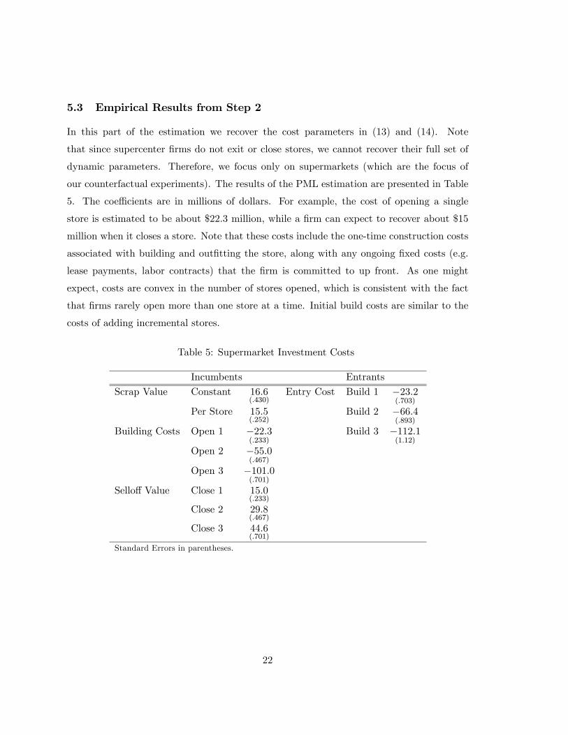
In this part of the estimation we recover the cost parameters in (13) and (14). Note

that since supercenter �rms do not exit or close stores, we cannot recover their full set of

dynamic parameters. Therefore, we focus only on supermarkets (which are the focus of

our counterfactual experiments). The results of the PML estimation are presented in Table

5. The coe¢ cients are in millions of dollars. For example, the cost of opening a single

store is estimated to be about $22.3 million, while a �rm can expect to recover about $15

million when it closes a store. Note that these costs include the one-time construction costs

associated with building and out�tting the store, along with any ongoing �xed costs (e.g.

lease payments, labor contracts) that the �rm is committed to up front. As one might

expect, costs are convex in the number of stores opened, which is consistent with the fact

that �rms rarely open more than one store at a time. Initial build costs are similar to the

costs of adding incremental stores.

Table 5: Supermarket Investment Costs

Incumbents Entrants

Scrap Value Constant 16:6(:430)

Entry Cost Build 1 �23:2(:703)

Per Store 15:5(:252)

Build 2 �66:4(:893)

Building Costs Open 1 �22:3(:233)

Build 3 �112:1(1:12)

Open 2 �55:0(:467)

Open 3 �101:0(:701)

Sello¤ Value Close 1 15:0(:233)

Close 2 29:8(:467)

Close 3 44:6(:701)


22

6 Policy Experiments

This section describes work that is currently in progress. For now, we simply provide a

road map intended to clarify the purpose of the estimators described above and their use

in conducting the policy experiments that constitute the central empirical contribution of

this paper.

The parameters and distributions estimated in the previous section will be used here as

inputs for a series of policy experiments. In particular, we will use a discrete control version

of the algorithm proposed in Pakes and McGuire (2001) (PM) to evaluate the impact of the

supercenter format on competition in the supermarket industry. The fact that Wal-Mart has

yet to close a store or exit entirely from an active market implies that we cannot recover

the full set of structural parameters that characterize Wal-Mart�s equilibrium behavior,

so even though we can estimate the model with both types of �rms, we cannot re-solve

for the equilibrium that was played in the data without imposing further assumptions.

Fortunately, our central counterfactual exercise � characterizing the change in consumer

surplus associated with eliminating the supercenter format altogether � only requires re-

solving the equilibrium for the players for whom we can recover the full set of structural

parameters: the conventional supermarket �rms. An estimate of the relevant baseline

comparison (consumer welfare with supercenters) is already available in the data. Our �rst

exercise is simply to compare the welfare estimates (and the resulting changes in market

structure) from the static and dynamic models.

Because our game involves controls that are entirely discrete, it is reasonably straightfor-

ward to implement a discrete control version of the stochastic PM algorithm in our context

(we are already using monte carlo integration as part of the estimation routine). This is

the key to accommodating a large state space with several players and a large number of

potential actions, a situation which would be intractable using the original (non-stochastic)

PM algorithm.

In addition to the elimination of the supercenter format, we will also consider sev-

eral other comparative dynamics aimed at characterizing the types of markets that are

most/least likely to incur supercenter entry, both in terms of consumer demographics and

incumbent market structures. Finally, by imposing some additional structure � namely,

23

assuming that Wal-Mart�s salvage values are proportional to those of conventional super-

markets11 �we can consider an even richer set of counterfactual exercises. In particular, we

can look at how policies that raise Wal-Mart�s �xed or marginal costs would impact both

consumer and producer surplus (as this involves re-solving the model with both types of

�rms).

A more comprehensive discussion will be added in a future version of the paper (once

the code for the stochastic PM algorithm is �nalized).

7 Conclusion

This paper proposes and estimates a model of dynamic competition in the supermarket

industry. Using recently developed two-step estimation techniques, we recover the struc-

tural parameters governing demand, pricing decisions, incremental investment, and entry

costs. We then use these parameter estimates to evaluate policies aimed at eliminating

supercenters.

11Speci�cally, we will assume that Wal-Mart can recover the same percentage of their (signi�cantly larger)initial investment as the conventional supermarket �rms do.

24

Table 6: Policy Parameters for Supermarket Incumbents

Dependent Variable Exit Close 3 Close 2 Close 1 Open 1 Open 2 Open 3

Own Store Density (dj) �15:12(1:22)

�:601(:645)

1:18(:526)

1:10(:256)

2:09(:234)

2:53(:403)

2:99(:538)

Rival Store Density��d�j�

6:72(1:14)

1:18(1:84)

2:09(1:53)

:268(:752)

�3:44(:614)

�5:05(1:04)

�5:04(1:21)

Supercenters�NSC

�:655(:093)

:547(:156)

:209(:141)

:267(:064)

�:808(:054)

�:250(:096)

�:328(:112)

Supermarkets�NSM

�:177(:049)

�:906(:077)

�:060(:068)

:024(:031)

�:137(:025)

�:294(:045)

�:323(:052)


�:440(:100)

�:549(:147)

�:479(:128)

�:544(:060)

:156(:053)

:170(:096)

:756(:125)


:586(:201)

�:238(:315)

�:066(:261)

:397(:123)

�:764(:103)

�1:29(:174)

�1:16(:206)

Population Growth �26:9(19:6)

�:281(32:7)

�38:6(31:6)

�11:6(13:4)

21:0(10:2)

36:1(17:2)

42:1(19:1)

Population �:002(:001)

:008(:003)

:007(:001)

:005(:001)

:006(:001)

:007(:001)

:008(:001)

Constant 22:8(19:8)

�4:22(38:9)

34:2(31:8)

8:58(13:5)

�22:7(10:3)

�38:4(17:4)

�44:9(19:2)

Log Likelihood �13174:1Observations 15239

Standard errors in parentheses. Baseline alternative is �do nothing�.

25

Table 7: Policy Parameters for Supercenter Incumbents

Dependent Variable Exit Open 1 Open 2 Open 3

Own Store Density (dj) �47:6(13:6)

�1:90(1:45)

�9:15(3:44)

5:20(3:31)


10:4(6:00)

:470(1:11)

�1:12(2:12)

�1:84(2:74)

Supercenters�NSC

�1:50(:448)

�:668(:151)

�:574(:263)

�:668(:357)

Supermarkets�NSM

�:155(:251)

�:084(:054)

�:025(:095)

:096(:114)


:512(:731)

�:509(:153)

�:629(:259)

�1:45(:286)


2:65(:956)

�:296(:185)

�:322(:351)

�:374(:457)

Population Growth 62:3(67:7)

3:17(22:4)

37:3(35:1)

85:4(43:9)


:006(:001)

:008(:001)

:014(:001)

Constant �68:2(69:3)

�3:59(22:6)

�39:1(35:5)

�90:0(44:1)

Log Likelihood -1726.3Observations 2273Standard errors in parentheses. Baseline alternative is �do nothing�.

Table 8: Policy Parameters for Supermarket Entrants

Dependent Variable Open 1 Open 2 Open 3


�8:01(2:38)

3:99(6:07)

�4:46(5:84)

Supercenters�NSC

��:463(:159)

:260(:467)

�:575(:601)

Supermarkets�NSM

��:148(:082)

�:220(:259)

�:474(:280)


�:553(:331)

:465(:981)

�2:65(:999)

Population Growth 26:9(28:3)

�77:6(111)

13:3(118)


�:006(:007)

�:001(:002)

Constant �26:7(28:6)

73:0(112)

�15:9(118)

Log Likelihood -724.2Observations 3312SEs in parentheses. Baseline alternative is �do not enter�.

26

Table 9: Policy Parameters for Supercenter Entrants

Dependent Variable Open 1 Open 2


�4:30(1:78)

�:856(:554)

Supercenters�NSC

��1:98(:191)

�2:55(:442)

Supermarkets�NSM

��:210(:073)

�:502(:152)


�1:03(:284)

:856(:554)

Population Growth �65:6(29:3)

�13:5(49:6)


�:002(:001)

Constant 66:1(29:5)

13:7(49:9)

Log Likelihood -841.2Observations 3312SEs in parentheses. Baseline alternative is �do not enter�.

References

Aguirregabiria, V., and P. Mira (2007): �Sequential Estimation of Dynamic Discrete

Games,�Econometrica, 75, 1�53.

Altug, S., and R. A. Miller (1998): �The E¤ect of Work Experience on Female Wages

and Labour Supply,�Review of Economic Studies, 62, 45�85.

Arcidiacono, P., and R. A. Miller (2008): �CCP Estimation of Dynamic Discrete

Choice Models with Unobserved Heterogeneity,�Working paper, Duke University.

Bajari, P., C. L. Benkard, and J. Levin (2007): �Estimating Dynamic Models of

Imperfect Competition,�Econometrica, 75, 1331�1370.

Bellman, R. E. (1957): Dynamic Programming. Princeton N.J.: Princeton University

Press.

Benkard, C. L. (2004): �A Dynamic Analysis of the Market for Wide-Bodied Commercial

Aircraft,�Review of Economic Studies, 71, 581�611.

27

Berry, S. (1992): �Estimation of a Model of Entry in the Airline Industry,�Econometrica,

60(4), 889�917.

(1994): �Estimating Discrete Choice Models of Product Di¤erentiation,� Rand

Journal of Economics, 25(2), 242�262.

Berry, S., J. Levinsohn, and A. Pakes (1995): �Automobile Prices in Market Equilib-

rium,�Econometrica, 63, 841�890.

Bresnahan, T. F., and P. C. Reiss (1987): �Do Entry Conditions Vary Across Mar-

kets?,�Brookings Papers on Economic Activity, pp. 833�871.

(1990): �Entry in Monopoly Markets,�Review of Economic Studies, 57, 531�553.

(1991a): �Empirical Models of Discrete Games,� Journal of Econometrics, 48,

57�82.

(1991b): �Entry and Competition in Concentrated Markets,�Journal of Political

Economy, 99(5), 977�1009.

Collard-Wexler, A. (2006): �Demand Fluctuations in the Ready-Mix Concrete Indus-

try,�New York University working paper.

Doraszelski, U., and M. Satterthwaite (2009): �Computable Markov-Perfect Indus-

try Dynamics,�Rand Journal of Economics, Forthcoming.

Dunne, T., S. Klimek, M. J. Roberts, and Y. Xu (2006): �Entry and Exit in Geo-

graphic Markets,�Penn State working paper.

Ellickson, P. B. (2006): �Quality Competition in Retailing: A Structural Analysis,�

International Journal of Industrial Organization, 24(3), 521�540.

(2007): �Does Sutton Apply to Supermarkets?,�Rand Journal of Economics, 38,

43�59.

Ericson, R., and A. Pakes (1995): �Markov-Perfect Industry Dynamics: A Framework

for Empirical Work,�Review of Economic Studies, 62, 53�82.

28

Hotz, V. J., and R. A. Miller (1993): �Conditional Choice Probabilities and the Esti-

mation of Dynamic Models,�Review of Economic Studies, 60, 497�529.

Hotz, V. J., R. A. Miller, S. Sanders, and J. Smith (1994): �A Simulation Estimator

for Dynamic Models of Discrete Choice,�Review of Economic Studies, 61, 265�289.

Mazzeo, M. (2002): �Product Choice and Oligopoly Market Structure,�Rand Journal of

Economics, 33, 221�242.

McFadden, D. L. (1984): �Econometric Analysis of Qualitative Response Models,� in

Handbook of Econometrics, ed. by Z. Griliches, and M. Intrilligator, vol. 2, chap. 24, pp.

1396�1456. Elsevier, Amsterdam.

Miller, R. A. (1997): �Estimating Models of Dynamic Optimization with Microeconomic

Data,� in Handbook of Applied Econometrics: Microeconomics, ed. by M. Pesaran, and

M. Schmidt, vol. 2, chap. 6, pp. 246�299. Blackwell, Oxford, U.K.

Pakes, A., and P. McGuire (1994): �Computing Markov-Perfect Nash Equilibria: Nu-

merical Implications of a Dynamic Di¤erentiated Product Model,�Rand Journal of Eco-

nomics, 25(4), 555�588.

(2001): �Stochastic Algorithms, Symmetric Markov Perfect Equilibrium, and the

�Curse of Dimensionality�,�Econometrica, 69(5), 1261�1281.

Pakes, A., M. Ostrovsky, and S. Berry (2007): �Simple Estimators for the Parame-

ters of Discrete Dynamic Games (with Entry/Exit Examples),�The RAND Journal of

Economics, 38, 373�399.

Pesendorfer, M., and P. Schmidt-Dengler (2007): �Asymptotic Least Squares Esti-

mators for Dynamic Games,�Review of Economic Studies, 75, 901�928.

Rust, J. (1987): �Optimal Replacement of GMC Bus Engines: An Empirical Model of

Harold Zurcher,�Econometrica, 55, 999�1013.

Ryan, S. (2004): �The Costs of Environmental Regulation in a Concentrated Industry,�

MIT Working Paper.

29

Seim, K. (2006): �An Empirical Model of Firm Entry with Endogenous Product-Type

Choices,�Rand Journal of Economics, 37, 619�640.

Smith, H. (2004): �Supermarket Choice and Supermarket Competition in Market Equi-

librium,�Review of Economic Studies, 71, 235�263.

Sweeting, A. (2007): �Dynamic Product Repositioning in Di¤erentiated Product Indus-

tries: The Case of Format Switching in the Commercial Radio Industry,�MIT Working

Paper.

30

the dynamics of retail oligopoly - paul.ellicksonpaulellickson.com/smdynamics.pdf · the dynamics...

Documents