the dual simplex method, techniques for a fast and stable
TRANSCRIPT
Dissertation
The Dual Simplex Method,
Techniques for a fast and stableimplementation
von
Dipl. Inform. Achim Koberstein
Schriftliche Arbeit zur Erlangung des akademischen Gradesdoctor rerum politicarum (dr. rer. pol.)
im Fach Wirtschaftsinformatik
eingereicht an derFakultat fur Wirtschaftswissenschaften der
Universitat Paderborn
Gutachter:1. Prof. Dr. Leena Suhl2. Prof. Dr. Michael Junger
Paderborn, im November 2005


To my family

v
Danksagungen
Die vorliegende Arbeit entstand in den vergangenen zweieinhalb Jahren, die ich alsStipendiat der International Graduate School of Dynamic Intelligent Systems amDecision Support & Operations Research (DSOR) Lab der Universitat Paderbornverbrachte. Ich mochte mich an dieser Stelle bei allen Menschen bedanken, die zumGelingen dieser Arbeit beigetragen haben.
Zuerst gilt mein besonderer und herzlicher Dank meinem ”Betreuerteam”, derLeiterin des DSOR-Labs Prof. Dr. Leena Suhl und ihrem Mann Prof. Dr. UweSuhl von der Freien Universitat Berlin. Leena Suhl danke ich fur das besondere Ver-trauensverhaltnis und die standige fachliche und personliche Unterstutzung. UweSuhl erwahnte zu Beginn meiner Promotionszeit eher beilaufig, dass der duale Sim-plexalgorithmus ein lohnenswertes Thema ware. Es ist vor allem ihm und seiner vo-rausgegangenen funfundzwanzigjahrigen Entwicklungsarbeit an dem Optimierungssys-tem MOPS zu verdanken, dass daraus dann tatsachlich eine Dissertation gewordenist. Die enge und lehrreiche Zusammenarbeit mit ihm hat mir großen Spaß gemachtund wird hoffentlich noch lange andauern.
Ich mochte mich außerdem bei allen Kollegen am DSOR-Lehrstuhl fur die guteZusammenarbeit und die anregende Forschungsatmosphare bedanken. Besondersmeiner Burokollegin Natalia Kliewer (inzwischen Juniorprofessorin) gebuhrt meinDank fur ihre freundschaftliche Unterstutzung, viele erhellende und erheiternde philo-sophisch-politische Gesprache uber die Monitore hinweg und ihre verstandnisvolleTeilnahme an privaten und beruflichen Hohenflugen und Tiefschlagen der letztendrei Jahre.
Ich danke auch der International Graduate School of Dynamic Intelligent Systems,insbesondere dem Leiter Dr. Eckhard Steffen und dem ganzen Organisationsteam furdie engagierte Begleitung meiner Arbeit, die weit uber die finanzielle Unterstutzunghinaus ging. Ich wunsche der IGS eine glanzende Zukunft und ihren jetzigen undkunftigen Stipendiaten eine erfolg- und lehrreiche Promotionszeit.
Ich danke allen, die mir bei der Korrektur des Manusskripts geholfen haben, ins-besondere Astrid Lukas-Reiß, Sophie Koberstein und Markus Krause.
Schließlich mochte ich mich bei meiner Frau Sophie sowie meinen Eltern, Schwie-gereltern und Freunden fur ihren Ruckhalt und ihre Unterstutzung bedanken. Durcheuch weiß ich jeden Tag, was wirklich wichtig ist.
Vielen herzlichen Dank!
Paderborn, im Oktober 2005 Achim Koberstein

vi
vii
Contents
1 Introduction 1
I Fundamental algorithms 5
2 Foundations 7
2.1 The linear programming problem and its computational forms . . . . 7
2.2 Geometry . . . . . . . . . . . . . . . . . . . . . . . . . . . . . . . . . 9
2.3 LP Duality . . . . . . . . . . . . . . . . . . . . . . . . . . . . . . . . 11
2.4 Basic solutions, feasibility, degeneracy and optimality . . . . . . . . . 13
3 The Dual Simplex Method 17
3.1 The Revised Dual Simplex Algorithm . . . . . . . . . . . . . . . . . . 17
3.1.1 Basic idea . . . . . . . . . . . . . . . . . . . . . . . . . . . . . 17
3.1.2 Neighboring solutions . . . . . . . . . . . . . . . . . . . . . . . 18
3.1.3 Pricing . . . . . . . . . . . . . . . . . . . . . . . . . . . . . . . 19
3.1.4 Ratio test . . . . . . . . . . . . . . . . . . . . . . . . . . . . . 20
3.1.5 Basis change . . . . . . . . . . . . . . . . . . . . . . . . . . . . 22
3.1.6 Algorithmic descriptions . . . . . . . . . . . . . . . . . . . . . 25
3.2 The Bound Flipping Ratio Test . . . . . . . . . . . . . . . . . . . . . 25
3.3 Dual steepest edge pricing . . . . . . . . . . . . . . . . . . . . . . . . 30
3.4 Elaborated version of the Dual Simplex Algorithm . . . . . . . . . . . 34
4 Dual Phase I Methods 37
4.1 Introduction . . . . . . . . . . . . . . . . . . . . . . . . . . . . . . . . 37
4.1.1 Big-M method . . . . . . . . . . . . . . . . . . . . . . . . . . . 37
4.1.2 Dual feasibility correction . . . . . . . . . . . . . . . . . . . . 37
4.2 Minimizing the sum of dual infeasibilities . . . . . . . . . . . . . . . . 38
4.2.1 Subproblem approach . . . . . . . . . . . . . . . . . . . . . . . 38
4.2.2 Algorithmic approach . . . . . . . . . . . . . . . . . . . . . . . 40
4.3 Artificial bounds . . . . . . . . . . . . . . . . . . . . . . . . . . . . . 45
4.4 Cost modification . . . . . . . . . . . . . . . . . . . . . . . . . . . . . 45
4.5 Pan’s method . . . . . . . . . . . . . . . . . . . . . . . . . . . . . . . 47
II Computational techniques 49
viii
5 Solving Systems of Linear Equations 515.1 Introduction . . . . . . . . . . . . . . . . . . . . . . . . . . . . . . . . 51
5.1.1 Product form of the inverse . . . . . . . . . . . . . . . . . . . 525.1.2 LU decomposition . . . . . . . . . . . . . . . . . . . . . . . . . 53
5.2 LU factorization . . . . . . . . . . . . . . . . . . . . . . . . . . . . . . 545.3 LU update . . . . . . . . . . . . . . . . . . . . . . . . . . . . . . . . . 56
5.3.1 Forrest/Tomlin update . . . . . . . . . . . . . . . . . . . . . . 575.3.2 Suhl/Suhl update . . . . . . . . . . . . . . . . . . . . . . . . . 59
5.4 Exploiting (hyper-)sparsity in FTran, BTran and LU-update . . . . . 615.4.1 Algorithms for sparse and hypersparse triangular systems . . . 615.4.2 FTran and BTran with Suhl/Suhl update . . . . . . . . . . . . 65
6 Numerical Stability and Degeneracy 676.1 Introduction . . . . . . . . . . . . . . . . . . . . . . . . . . . . . . . . 67
6.1.1 Numerical stability . . . . . . . . . . . . . . . . . . . . . . . . 676.1.2 Degeneracy and cycling . . . . . . . . . . . . . . . . . . . . . . 69
6.2 Techniques to ensure numerical stability . . . . . . . . . . . . . . . . 706.2.1 Numerical tolerances . . . . . . . . . . . . . . . . . . . . . . . 706.2.2 Stabilizing ratio tests . . . . . . . . . . . . . . . . . . . . . . . 71
6.2.2.1 Modified standard ratio test . . . . . . . . . . . . . . 726.2.2.2 Harris’ ratio test . . . . . . . . . . . . . . . . . . . . 736.2.2.3 Shifting . . . . . . . . . . . . . . . . . . . . . . . . . 746.2.2.4 Stabilizing bound flipping ratio test . . . . . . . . . . 75
6.2.3 Refactorization, accuracy checks and stability control . . . . . 776.2.3.1 Refactorization for speed . . . . . . . . . . . . . . . . 776.2.3.2 Refactorization for stability . . . . . . . . . . . . . . 79
6.3 Techniques to reduce degeneracy and prevent cycling . . . . . . . . . 826.3.1 Perturbation . . . . . . . . . . . . . . . . . . . . . . . . . . . . 826.3.2 Randomized pricing . . . . . . . . . . . . . . . . . . . . . . . . 84
7 Further computational aspects 857.1 LP preprocessing, scaling and crash procedures . . . . . . . . . . . . 857.2 Computation of the pivot row . . . . . . . . . . . . . . . . . . . . . . 87
III Implementation and results 89
8 Implementation 918.1 The Mathematical OPtimization System MOPS . . . . . . . . . . . . 91
8.1.1 MOPS and its history . . . . . . . . . . . . . . . . . . . . . . 918.1.2 External system architecture . . . . . . . . . . . . . . . . . . . 928.1.3 LP / MIP solution framework . . . . . . . . . . . . . . . . . . 93
8.2 The dual simplex code . . . . . . . . . . . . . . . . . . . . . . . . . . 968.2.1 Basic data structures . . . . . . . . . . . . . . . . . . . . . . . 968.2.2 Pricing . . . . . . . . . . . . . . . . . . . . . . . . . . . . . . . 98
8.2.2.1 Initialization and update of DSE weights . . . . . . . 98
ix
8.2.2.2 Vector of primal infeasibilities . . . . . . . . . . . . . 1008.2.2.3 Partial randomized pricing . . . . . . . . . . . . . . . 101
8.2.3 Ratio test . . . . . . . . . . . . . . . . . . . . . . . . . . . . . 1018.2.4 FTran, BTran, LU-Update and factorization . . . . . . . . . . 103
8.2.4.1 Data structures for the LU-factors . . . . . . . . . . 1048.2.4.2 Exploiting hypersparsity . . . . . . . . . . . . . . . . 1068.2.4.3 Forward Transformation (FTran) . . . . . . . . . . . 1088.2.4.4 LU-update and factorization . . . . . . . . . . . . . . 113
8.2.5 Overview . . . . . . . . . . . . . . . . . . . . . . . . . . . . . 114
9 Numerical results 1179.1 Test problems . . . . . . . . . . . . . . . . . . . . . . . . . . . . . . . 1179.2 Performance measures . . . . . . . . . . . . . . . . . . . . . . . . . . 1189.3 Study on dual phase 1 . . . . . . . . . . . . . . . . . . . . . . . . . . 1189.4 Chronological progress study . . . . . . . . . . . . . . . . . . . . . . . 1219.5 Overall benchmarks . . . . . . . . . . . . . . . . . . . . . . . . . . . . 124
10 Summary and Conclusion 129
Bibliography 131
A Tables 137

x
xi
List of Figures
2.1 A convex polyhedron in R2. . . . . . . . . . . . . . . . . . . . . . . . 9
5.1 Forrest/Tomlin update . . . . . . . . . . . . . . . . . . . . . . . . . . 585.2 Suhl/Suhl update . . . . . . . . . . . . . . . . . . . . . . . . . . . . . 605.3 An upper triangular matrix an the corresponding nonzero graph G . . 64
8.1 The external architecture of MOPS . . . . . . . . . . . . . . . . . . . 948.2 LP/IP solution framework in MOPS . . . . . . . . . . . . . . . . . . 958.3 Columnwise compact storage for A before and after LP preprocessing. 968.4 Dense, indexed and packed storage for mathematical vectors. . . . . . 978.5 Implementation of the bound flipping ratio test with Harris’ tolerance. 1028.6 Data structure for U . . . . . . . . . . . . . . . . . . . . . . . . . . . . 1048.7 Data structure for the eta vectors of L−1 (1). . . . . . . . . . . . . . . 1058.8 Data structure for the eta vectors of L−1 (2). . . . . . . . . . . . . . . 1068.9 Data structure for depth-first-search. . . . . . . . . . . . . . . . . . . 1078.10 Data-flow of FTran operation. . . . . . . . . . . . . . . . . . . . . . . 1088.11 Implementation overview: initialization, refactorization and dual phase
I. . . . . . . . . . . . . . . . . . . . . . . . . . . . . . . . . . . . . . . 1158.12 Implementation overview: main loop. . . . . . . . . . . . . . . . . . . 116
9.1 Performance profile over phase 1 test set: solution time using fourdifferent dual phase 1 methods. . . . . . . . . . . . . . . . . . . . . . 120
9.2 Performance profile over all test models: solution time with reducedand expanded bounds after LP preprocessing. . . . . . . . . . . . . . 121
9.3 Chronological progress in the development process of the MOPS DualSimplex code. . . . . . . . . . . . . . . . . . . . . . . . . . . . . . . . 123
9.4 Overall benchmarks. . . . . . . . . . . . . . . . . . . . . . . . . . . . 125

xii
xiii
List of Tables
2.1 Primal-dual transformation rules. . . . . . . . . . . . . . . . . . . . . 122.2 Dual feasibility conditions. . . . . . . . . . . . . . . . . . . . . . . . . 15
6.1 Tolerances: notation and default values. . . . . . . . . . . . . . . . . 71
8.1 History of MOPS development. . . . . . . . . . . . . . . . . . . . . . 928.2 Improvement of MOPS LP optimization on model oil. . . . . . . . . . 928.3 Improvement of MOPS IP optimization on model oil. . . . . . . . . . 93
9.1 Benchmark of dual phase 1 methods. . . . . . . . . . . . . . . . . . . 1199.2 Benchmark with reduced and expanded bounds after LP-preprocessing
on original test set. . . . . . . . . . . . . . . . . . . . . . . . . . . . . 1219.3 Progress in our dual simplex code: implementation techniques in
chronological order. . . . . . . . . . . . . . . . . . . . . . . . . . . . . 1229.4 System benchmark: solution time (including time for LP preprocess-
ing) on 25 most difficult original models. . . . . . . . . . . . . . . . . 1269.5 Benchmark of dual simplex codes (no LP preprocessing): solution
time on 25 most difficult models pretreated by COIN LP preprocessing.127
A.1 Model dimensions. . . . . . . . . . . . . . . . . . . . . . . . . . . . . 139A.2 Results with Cplex 9.1 Dual Simplex. . . . . . . . . . . . . . . . . . . 141A.3 Results with COIN LP 1.02.02 Dual Simplex. . . . . . . . . . . . . . 143A.4 Results with Soplex 1.2.1 Dual Simplex. . . . . . . . . . . . . . . . . 145A.5 Results with MOPS 7.9 Dual Simplex. . . . . . . . . . . . . . . . . . 147A.6 Results with MOPS 7.9 Dual Simplex with expanded bounds after LP
preprocessing. . . . . . . . . . . . . . . . . . . . . . . . . . . . . . . . 149A.7 Results on Dual Phase 1: Combined Method ”Pan + Subproblem-
Approach”. . . . . . . . . . . . . . . . . . . . . . . . . . . . . . . . . 150A.8 Results on Dual Phase 1: Pan’s method. . . . . . . . . . . . . . . . . 151A.9 Results on Dual Phase 1: Minimization of the sum of dual infeasibil-
ities, subproblem approach. . . . . . . . . . . . . . . . . . . . . . . . 152A.10 Results on Dual Phase 1: Cost modification + Primal Simplex. . . . . 153A.11 Progress in our dual simplex code: implementation techniques in
chronological order. . . . . . . . . . . . . . . . . . . . . . . . . . . . . 154A.12 Chronological progress: solution time. . . . . . . . . . . . . . . . . . . 155A.13 Chronological progress: total iteration count. . . . . . . . . . . . . . . 156

xiv

xv
List of Algorithms
1 Basic steps of the dual simplex method. . . . . . . . . . . . . . . . . . . . 172 Dual simplex method with simple ratio test and update of d. . . . . . . . . 263 Dual simplex method with simple ratio test and update of y. . . . . . . . . 274 Selection of q with the BRFT. . . . . . . . . . . . . . . . . . . . . . . . . . 315 Update of d and xB for the BRFT. . . . . . . . . . . . . . . . . . . . . . . 316 Update of xN for the BRFT. . . . . . . . . . . . . . . . . . . . . . . . . . . 317 Dual simplex method with dual steepest edge pricing, bound flipping ratio
test and update of d. . . . . . . . . . . . . . . . . . . . . . . . . . . . . . . 358 The 2-phases dual simplex method with subproblem dual phase I. . . . . . 409 Dual phase 1: Minimizing the sum of dual infeasibilities with simple ratio
test. . . . . . . . . . . . . . . . . . . . . . . . . . . . . . . . . . . . . . . . 4310 Extended ratio test in dual phase I. . . . . . . . . . . . . . . . . . . . . . . 4611 Dual phase 1: Pan’s method. . . . . . . . . . . . . . . . . . . . . . . . . . 4812 LU-factorization. . . . . . . . . . . . . . . . . . . . . . . . . . . . . . . . . 5513 LU-Update Suhl/Suhl (in terms of U) . . . . . . . . . . . . . . . . . . . . 6214 Ux = b – dense method (for dense b) . . . . . . . . . . . . . . . . . . . . . 6315 Ux = b – sparse method (for sparse b) . . . . . . . . . . . . . . . . . . . . 6316 Ux = b – hyper-sparse method (for very sparse x) . . . . . . . . . . . . . . 6517 Modified standard ratio test . . . . . . . . . . . . . . . . . . . . . . . . . . 7218 Bound flipping ratio test with Harris’ tolerance. . . . . . . . . . . . . . . . 7819 HypersparsityTest . . . . . . . . . . . . . . . . . . . . . . . . . . . . . . . . 10720 FTran (Pseudocode) . . . . . . . . . . . . . . . . . . . . . . . . . . . . . . 10921 FTranL-F sparse . . . . . . . . . . . . . . . . . . . . . . . . . . . . . . . . 11022 FTranL-U . . . . . . . . . . . . . . . . . . . . . . . . . . . . . . . . . . . . 11023 FTranU sparse() . . . . . . . . . . . . . . . . . . . . . . . . . . . . . . . . 11124 FTranU hyper . . . . . . . . . . . . . . . . . . . . . . . . . . . . . . . . . . 11125 FTranU hyper DFS . . . . . . . . . . . . . . . . . . . . . . . . . . . . . . . 112

xvi
1
Chapter 1
Introduction
In 1947, G.B. Dantzig stated the Linear Programming Problem (LP) and presentedthe (primal) simplex method1 to solve it (cf. [18, 19, 21]). Since then many re-searchers have strived to advance his ideas and made linear programming the mostfrequently used optimization technique in science and industry. Besides the inves-tigation of the theoretical properties of the simplex method the development ofincreasingly powerful computer codes has always been a main goal of research inthis field. Boosted by the performance leaps of computer hardware, the continuousimprovement of its algorithmic and computational techniques is probably the mainreason for the success story of the simplex method. Orden [52] and Hoffmann [35]were among the first to report computational results for their codes. In 1952, anLP problem with 48 constraints and 71 variables took about 18 hours and 73 sim-plex iterations to solve on a SEAC computer, which was the hardware available atthat time. The most difficult test problem2 used in this dissertation has 162,142constraints and 1,479,833 variables and is solved by our dual simplex code in about7 hours and about 422,000 simplex iterations on a standard personal computer (seechapter 9). More information about the history of linear programming and LP com-puter codes can be found in [43] and [51], respectively.
While the primal simplex algorithm was in the center of research interest fordecades and subject of countless publications, this was not the case regarding itsdual counterpart. After Lemke [42] had presented the dual simplex method in 1954,it was not considered to be a competitive alternative to the primal simplex methodfor nearly forty years. Commercial LP-systems of the late 1980s like MPSX/370,MPS III or APEX-III featured only rudimentary implementations of it and did noteven include dual phase I methods to deal with dual infeasible starting bases (cf. [10]).This eventually changed in the early 1990s mainly due to the contributions of Forrestand Goldfarb [26], who developed a computationally relatively cheap dual version ofthe steepest edge pricing rule.
During the last decade commercial solvers made great progress in establishing thedual simplex method as a general solver for large-scale LP problems. Nowadays,large scale LP problems can be solved either by an interior point, primal simplexor dual simplex algorithm or a combination of such algorithms. In fact, extensivecomputational studies indicate, that the overall performance of the dual simplex
1The historic circumstances of the early days of linear programming have been documented e.g.by S.I. Gass [28] and A.J. Hoffman [36].
2LP-relaxation of the integer problem MUN1 M D, which is an instance of multi-commodity-flowmodel used in a bus scheduling application [37].
2 Chapter 1 Introduction
may be superior to that of the primal simplex algorithm (cf. [10]). In practise, thereare often LP-models, for which one of the three methods clearly outperforms theothers. For instance, experiments showed, that the test problem mentioned abovecan only be solved by the dual simplex method. Primal simplex codes do virtuallynot converge on this problem due to degeneracy and interior point codes fail due toextensive memory consumption.
Besides its relevance for the solution of large scale LP problems, it is long known,that the dual simplex algorithm plays an important role for solving LP problems,where some or all of the variables are constrained to integer values (mixed-integerlinear programming problems – MIPs). Virtually all state-of-the-art MIP-solvers arebased on a branch-and-bound approach, where dual bounds on the objective functionvalue are computed by successive reoptimization of LP-type subproblems. While theinterior-point method is conceptually ineligible to take advantage of a given nearlyoptimal starting solution, the dual simplex method is particularly well suited for thispurpose. The reason is that for most of the branch-and-bound subproblems the lastLP-solution stays dual feasible and the execution of a dual phase I method is notnecessary. Therefore, the dual simplex method is typically far superior to the primalsimplex method in a branch-and-bound framework.
Despite of its success and relevance for future research only few publications inresearch literature explicitly discuss implementation details of mathematical or com-putational techniques proposed for the dual simplex algorithm. Furthermore, re-ported computational results are often produced by out-dated simplex codes, whichdo not feature indispensable techniques to solve large scale LPs (like a well imple-mented LU factorization of the basis and a powerful LP preprocessor). Even if thepresented ideas look promising, it often remains unclear, how to implement themwithin a state-of-the-art LP-system. Such techniques are for example:
• An enhanced dual ratio test for dual phase I and phase II. It was described byFourer [27] in an unpublished rather theoretical note about the dual simplexmethod3. Maros [48, 47] and Kostina [41] published computational results forthis technique.
• Pan’s dual phase I method. Pan presented his algorithm in [54] and publishedcomputational results in [55].
• A method to exploit hypersparsity. In the mid 1980’s Gilbert and Peierls [29]published a technique to solve particularly sparse systems of linear equations.In [10] Bixby indicates that this technique contributed to enormous improve-ments of the Cplex LP-solver. However, he does not disclose implementationdetails.
The lack of descriptions of implementation details in the research literature has ledto a great performance gap between open-source research codes4 and commercial LP-
3Apparently, the idea was published long before by Gabasov [57] in Russian language.4An exception is the LP code, which is being developed in the COIN open-source initiave [44].
However, this code is largely undocumented and no research papers have yet been publishedabout its internals.
3
systems, which is frequently documented in independent benchmarks of optimizationsoftware (cf. [4]).
The goals of this dissertation follow directly from the above discussion. We think,that it is essential for future research in the field of linear and mixed integer program-ming to dispose of a state-of-the art implementation of the dual simplex algorithm.Therefore, we want
• to develop a dual simplex code, which is competitive to the best existing open-source and commercial LP-systems,
• to identify, advance and document important implementation techniques, whichare responsible for the superiority of commercial simplex codes, and
• to conduct meaningful computational studies to evaluate promising mathemat-ical and computational techniques.
Our work is based on the Mathematical OPtimization System (MOPS) (see [65, 66]),which has been deployed in many practical applications for over two decades (seee.g. [69], [67], [62] and [37]) and has continuously been improved in algorithms, soft-ware design and implementation. The system started as a pure LP-solver based on ahigh speed primal simplex algorithm. In its present form MOPS belongs to the fewcompetitive systems in the world to solve large-scale linear and mixed integer pro-gramming problems. The algorithms and computational techniques used in MOPShave been documented in numerous scientific publications (cf. section 8.1).
The remainder of this thesis is structured in three major parts. In part I, whichcomprises the chapters 2 to 4, we give a detailed description of the relevant mathe-matical algorithms. In chapter 2 we introduce fundamental concepts of linear pro-gramming. Chapter 3 gives a detailed derivation of the dual simplex method. Thechapter ends with an algorithmic description of an elaborate version of the algorithm,which represents the basis of the dual phase II part of our implementation. In chap-ter 4 we give an overview of dual phase I algorithms. In particular, we show thatthere are two mathematically equivalent approaches to minimize the sum of dualinfeasibilities and give the first algorithmic description of Pan’s method for generalLPs with explicit lower and upper bounds.
In part II, we describe computational techniques, which are crucial for the perfor-mance and numerical stability of our code. Here, the efficient solution of the requiredsystems of linear equations in chapter 5 plays an important role. We particularly em-phasize the exploitation of hypersparsity. Techniques to achieve numerical stabilityand prevent degeneracy and cycling are presented in chapter 6. We discuss in detail,how to combine Harris’ idea to use tolerances to improve numerical stability with thebound flipping ratio test. The shorter chapter 7 is concerned with further importantpoints, e.g. LP preprocessing and the efficient computation of the transformed pivotrow.
Part III comprises the chapters 8 and 9. The first describes our implementationof the mathematical algorithms and computational techniques presented in the pre-vious parts. Focal points are efficient data structures, organization of the pricingloop, the dual ratio test and the exploitation of hypersparsity. In the second chapter

4 Chapter 1 Introduction
of this part we evaluate the performance of our code compared to the best commer-cial and open-source implementations of the dual simplex method on the basis ofcomputational results. Furthermore, we provide a study on the dual phase I and achronological progress study, which illustrates the impact of the specific implemen-tation techniques on the overall performance of the code during our developmentprocess.
Chapter 10 summarizes the contributions of this dissertation and discusses possibledirections of future research.
5
Part I
Fundamental algorithms

7
Chapter 2
Foundations
2.1 The linear programming problem and itscomputational forms
A linear programming problem (LP) is the problem of minimizing (or maximizing)a linear function subject to a finite number of linear constraints. In matrix notationthis definition corresponds to the following general form of the LP problem:
minimize c0 + cTx (2.1a)
subject to L ≤ Ax ≤ U (2.1b)
l ≤ x ≤ u, (2.1c)
where c0 ∈ R, c, x ∈ Rn, b ∈ Rm, A ∈ Rm×n, l, u ∈ (R ∪ {−∞,+∞})n andL,U ∈ (R∪{−∞,+∞})m with m, n ∈ N. We call c the cost vector (c0 is a constantcomponent), x the vector of the decision variables, A the constraint matrix, L andU the (lower and upper) range vectors and l and u the (lower and upper) bounds.(2.1a) is called objective function, (2.1b) the set of joint constraints and (2.1c) theindividual bound constraints. We call a variable xj with j ∈ {1, . . . , n} free if lj = −∞and uj = +∞. We call it boxed if lj > −∞ and uj < +∞. If lj = uj = a for somea ∈ R we call it fixed.
It is easy to see that any kind of LP problem that may occur in a practicalapplication can be put into general form (2.1). If for i ∈ {1, . . . ,m} we have bothLi > −∞ and Ui < +∞ constraint i is a range constraint. If Li > −∞ and Ui = +∞or Li = −∞ and Ui < +∞ constraint i is an inequality-constraint (≥ or ≤ resp.). If−∞ < Li = Ui < +∞ it is an equality-constraint.
To be approachable by the simplex algorithm LP (2.1) has to be cast into acomputational form, that fulfills further requirements, i.e., the constraint matrix hasto have full row rank and only equality constraints are allowed:
min cTx (2.2a)
s.t. Ax = b (2.2b)
l ≤ x ≤ u. (2.2c)
Here, c, x ∈ Rn, b ∈ Rm, l, u ∈ (R∪{−∞,+∞})n and A ∈ Rm×n with rank(A) = m,m,n ∈ N and m < n. In this representation we call b the right hand side (RHS)vector. In the following we will denote by J = {1, . . . , n} the set of column indices.
8 Chapter 2 Foundations
To put an LP in general form (2.1) into one in computational form (2.2) inequal-ity constraints are transformed into equality constraints by introducing slack- andsurplus-variables. In LP-systems (like MOPS) this is usually done in a standardizedway by adding a complete identity matrix to the constraint matrix:
min cTxS (2.3a)
s.t.[A | I
] [xS
xL
]= 0 (2.3b)
l ≤[xS
xL
]≤ u (2.3c)
The variables associated with A are called structural variables (short: structurals),those associated with I are called logical variables (short: logicals). Ranges Li andUi are transferred to individual bounds on logical variables by setting ln+i = −Ui
and un+i = −Li. Consequently, equality constraints lead to fixed logical variables.Note, that this scheme assures that both the full row rank assumption (because ofI) and the requirement that m < n (since n = n + m) are fulfilled. We call (2.3)the internal model representation (IMR) while the general form (2.1) is also calledexternal model representation (EMR).
For ease of notation we will mostly use the computational form (2.2) to describemathematical methods and techniques. We will always assume that it coincides withthe IMR (2.3). One obvious computational advantage of the IMR is for instance,that the right hand side vector b is always 0, which means that it vanishes completelyin implementation. Nevertheless, we consider b in the algorithmic descriptions.
To examine the theoretical properties of LPs and also for educational purposes, aneven simpler yet mathematically equivalent representation is used in LP literature.It is well known that every LP can be converted into the following standard form:
min cTx (2.4a)
s.t. Ax ≥ b (2.4b)
x ≥ 0. (2.4c)
The set X = {x ∈ Rn : Ax ≥ b, x ≥ 0} is called the feasible region of the LP (2.4)and x ∈ Rn is called feasible if x ∈ X . If for every M ∈ R there is an x ∈ Xsuch that cTx < M , then (2.4) is called unbounded. If X = ∅ it is called infeasible.Otherwise, an optimal solution x∗ ∈ X exists with objective function value z∗ = cTx∗
and z∗ ≤ cTx for all x ∈ X .The simplex algorithm was originally developed for LPs in standard form (without
taking individual bounds into account implicitly). To apply the simplex algorithmto (2.4) it has to be transformed as above to a form which we will call computationalstandard form:
min cTx (2.5a)
s.t. Ax = b (2.5b)
x ≥ 0, (2.5c)
2.2 Geometry 9
G5
G4
G3
G2
G1
x1
x2
X
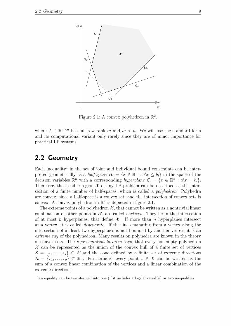
Figure 2.1: A convex polyhedron in R2.
where A ∈ Rm×n has full row rank m and m < n. We will use the standard formand its computational variant only rarely since they are of minor importance forpractical LP systems.
2.2 Geometry
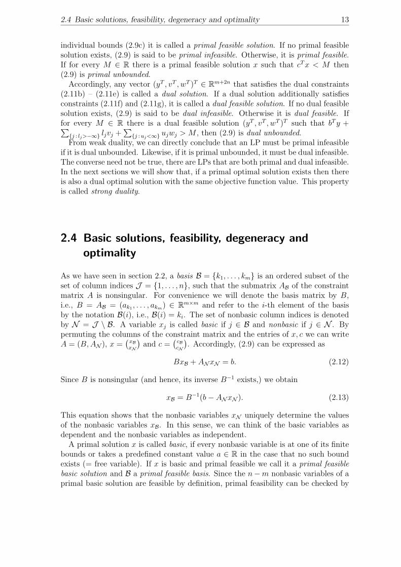
Each inequality1 in the set of joint and individual bound constraints can be inter-preted geometrically as a half-space Hi = {x ∈ Rn : aix ≤ bi} in the space of thedecision variables Rn with a corresponding hyperplane Gi = {x ∈ Rn : aix = bi}.Therefore, the feasible region X of any LP problem can be described as the inter-section of a finite number of half-spaces, which is called a polyhedron. Polyhedraare convex, since a half-space is a convex set, and the intersection of convex sets isconvex. A convex polyhedron in R2 is depicted in figure 2.1.
The extreme points of a polyhedron X , that cannot be written as a nontrivial linearcombination of other points in X , are called vertices. They lie in the intersectionof at most n hyperplanes, that define X . If more than n hyperplanes intersectat a vertex, it is called degenerate. If the line emanating from a vertex along theintersection of at least two hyperplanes is not bounded by another vertex, it is anextreme ray of the polyhedron. Many results on polyhedra are known in the theoryof convex sets. The representation theorem says, that every nonempty polyhedronX can be represented as the union of the convex hull of a finite set of verticesS = {s1, . . . , sk} ⊆ X and the cone defined by a finite set of extreme directionsR = {r1, . . . , rq} ⊂ Rn. Furthermore, every point x ∈ X can be written as thesum of a convex linear combination of the vertices and a linear combination of theextreme directions:
1an equality can be transformed into one (if it includes a logical variable) or two inequalities
10 Chapter 2 Foundations
x =k∑
i=1
λisi +
q∑j=1
µjrj, withk∑
i=1
λi = 1, λi ≥ 0 ∀i and µj ≥ 0 ∀j. (2.6)
With the help of this theorem one can proof a fundamental property of LP problems:for every LP problem exactly one of the following three solution states is true (seee.g. [46], p.25 for proof):
• The LP is infeasible. No feasible solution exists (X = ∅).
• The LP is unbounded. There is a vertex si ∈ S, an extreme direction rj ∈ Rsuch that for everyM ∈ R we can find a value µ ≥ 0 such that x∗ = si+µrj ∈ Xand cTx∗ < M .
• The LP has an optimal solution. There is an optimal vertex x∗ ∈ S such thatcTx∗ ≤ cTx for all x ∈ X .
Accordingly, if an LP problem has an optimal solution, it suffices to search the (finitenumber of) vertices of the feasible region until a vertex with the optimal solutionvalue is found. From the two possible definitions of a vertex two different algebraicrepresentations can be derived. Defining a vertex as the intersection of hyperplanesleads to the concept of a row basis. We will not further pursue this concept, sincein most cases it is computationally inferior to the concept of a column basis, whichfollows from the vertex definition via nontrivial convex combinations.
Suppose, we have an LP given in computational standard form and X = {x ∈ Rn :Ax = b, x ≥ 0}. A point x ∈ X is a vertex if and only if the column vectors of A, thatare associated with strictly positive entries in x, are linearly independent (see e.g. [16], p.9 for proof). As a direct consequence x can have at most m positive entries. If xhas strictly less than m positive entries, we can always expand the number of linearlyindependent columns to m by adding columns associated with zero positions of x,since A has full row rank (in this case, the vertex is degenerate). Therefore, everyvertex of the feasible region has at least one set of m linearly independent columns ofA associated with it. The set of indices of these columns is called a (column) basis.Consequently, degenerate vertices have several bases.
The fundamental idea of the simplex algorithm is to search the finite number ofbases until a basis is found that belongs to the optimal vertex. Since there are
(mn
)bases, this might take an exponential number of steps, which is in fact the theoreticalbound for the runtime of the method. In practise, it has surprisingly turned out toperform much better (typically c ∗m number of steps, where c is a small constant).It has been learned, that the performance heavily depends on sophisticated searchstrategies.
2.3 LP Duality 11
2.3 LP Duality
The basic idea of LP duality can be seen best by considering an LP in standard form:
z∗ = min cTx
s.t. Ax ≥ b
x ≥ 0.
(2.7)
If we multiply every constraint i ∈ {1, . . . ,m} with a nonnegative number yi suchthat yTaj ≤ cj for every j ∈ {1, . . . , n}, then yT b is a lower bound on the optimalobjective function value z∗, since yT b ≤ yTAx ≤ cTx (the first relation is true,because y ≥ 0, the second is true, because x ≥ 0 and yTaj ≤ cj). This property iscalled weak duality. Since it is satisfied by every y satisfying the restrictions abovewe can find the best lower bound by solving the LP:
Z∗ = max bTy
s.t. ATy ≤ c
y ≥ 0.
(2.8)
This LP is called the dual LP (or short: the dual) of the LP (2.7). Both LPs arecalled a primal-dual pair. Since any LP problem can be transformed into standardform, we can associate a dual problem to it in the above sense.
Consider a primal constraint aix ≤ bi. By multiplying by −1, we get −ai ≥ −bi,which is a constraint in standard form. In the dual program, a dual multiplier yi ≥ 0gets assigned to it and −bi becomes its coefficient in the dual objective function,while −(ai)T becomes its coefficient (column) in the dual constraint matrix. This isequivalent to assigning a dual multiplier yi ≤ 0 right away and keeping bi and (ai)T ascoefficients in the dual objective function and constraint matrix respectively. Primalequality constraints aix = bi can be replaced by two inequality constraints aix ≥ biand ai ≤ bi. In the dual program two dual variables y1
i ≥ 0 and y2i ≤ 0 go with
them, which have identical coefficients bi and (ai)T in the dual objective functionand constraint matrix respectively. Hence, the coefficients can be factored out givingbi(y
1i + y2
i ) and (ai)T (y1i + y2
i ) respectively. The sum y1i + y2
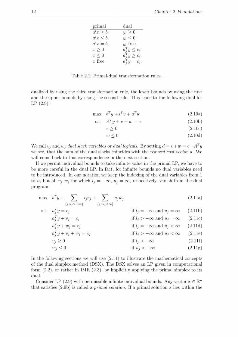
i can assume any valuein R, so it can be substituted by a free dual variable yi. In a similar manner wecan derive further transformation rules for different types of primal variables. Wesummarize them in table 2.1.
Now, reconsider an LP in computational form and suppose in the first instance,that all individual bounds are finite, i.e., lj > −∞ and uj <∞ for all j ∈ J :
min cTx (2.9a)
s.t. Ax = b (2.9b)
l ≤ x ≤ u. (2.9c)
Then, we can treat the individual bounds (2.9c) like constraints and introduce dualvariables y ∈ Rm for the constraints (2.9b), v ∈ Rn for the lower bound constraintsand w ∈ Rn for the upper bound constraints in (2.9c). The constraints (2.9b) can be
12 Chapter 2 Foundations
primal dualaix ≥ bi yi ≥ 0aix ≤ bi yi ≤ 0aix = bi yi freex ≥ 0 aT
j y ≤ cjx ≤ 0 aT
j y ≥ cjx free aT
j y = cj
Table 2.1: Primal-dual transformation rules.
dualized by using the third transformation rule, the lower bounds by using the firstand the upper bounds by using the second rule. This leads to the following dual forLP (2.9):
max bTy + lTv + uTw (2.10a)
s.t. ATy + v + w = c (2.10b)
v ≥ 0 (2.10c)
w ≤ 0 (2.10d)
We call vj and wj dual slack variables or dual logicals. By setting d = v+w = c−ATywe see, that the sum of the dual slacks coincides with the reduced cost vector d. Wewill come back to this correspondence in the next section.
If we permit individual bounds to take infinite value in the primal LP, we have tobe more careful in the dual LP. In fact, for infinite bounds no dual variables needto be introduced. In our notation we keep the indexing of the dual variables from 1to n, but all vj, wj for which lj = −∞, uj = ∞, respectively, vanish from the dualprogram:
max bTy +∑
{j : lj>−∞}
ljvj +∑
{j : uj<∞}
ujwj (2.11a)
s.t. aTj y = cj if lj = −∞ and uj =∞ (2.11b)
aTj y + vj = cj if lj > −∞ and uj =∞ (2.11c)
aTj y + wj = cj if lj = −∞ and uj <∞ (2.11d)
aTj y + vj + wj = cj if lj > −∞ and uj <∞ (2.11e)
vj ≥ 0 if lj > −∞ (2.11f)
wj ≤ 0 if uj < −∞ (2.11g)
In the following sections we will use (2.11) to illustrate the mathematical conceptsof the dual simplex method (DSX). The DSX solves an LP given in computationalform (2.2), or rather in IMR (2.3), by implicitly applying the primal simplex to itsdual.
Consider LP (2.9) with permissible infinite individual bounds. Any vector x ∈ Rn
that satisfies (2.9b) is called a primal solution. If a primal solution x lies within the
2.4 Basic solutions, feasibility, degeneracy and optimality 13
individual bounds (2.9c) it is called a primal feasible solution. If no primal feasiblesolution exists, (2.9) is said to be primal infeasible. Otherwise, it is primal feasible.If for every M ∈ R there is a primal feasible solution x such that cTx < M then(2.9) is primal unbounded.
Accordingly, any vector (yT , vT , wT )T ∈ Rm+2n that satisfies the dual constraints(2.11b) – (2.11e) is called a dual solution. If a dual solution additionally satisfiesconstraints (2.11f) and (2.11g), it is called a dual feasible solution. If no dual feasiblesolution exists, (2.9) is said to be dual infeasible. Otherwise it is dual feasible. Iffor every M ∈ R there is a dual feasible solution (yT , vT , wT )T such that bTy +∑
{j : lj>−∞} ljvj +∑
{j : uj<∞} ujwj > M , then (2.9) is dual unbounded.From weak duality, we can directly conclude that an LP must be primal infeasible
if it is dual unbounded. Likewise, if it is primal unbounded, it must be dual infeasible.The converse need not be true, there are LPs that are both primal and dual infeasible.In the next sections we will show that, if a primal optimal solution exists then thereis also a dual optimal solution with the same objective function value. This propertyis called strong duality.
2.4 Basic solutions, feasibility, degeneracy andoptimality
As we have seen in section 2.2, a basis B = {k1, . . . , km} is an ordered subset of theset of column indices J = {1, . . . , n}, such that the submatrix AB of the constraintmatrix A is nonsingular. For convenience we will denote the basis matrix by B,i.e., B = AB = (ak1 , . . . , akm) ∈ Rm×m and refer to the i-th element of the basisby the notation B(i), i.e., B(i) = ki. The set of nonbasic column indices is denotedby N = J \ B. A variable xj is called basic if j ∈ B and nonbasic if j ∈ N . Bypermuting the columns of the constraint matrix and the entries of x, c we can writeA = (B,AN ), x =
(xBxN
)and c =
(cBcN
). Accordingly, (2.9) can be expressed as
BxB + ANxN = b. (2.12)
Since B is nonsingular (and hence, its inverse B−1 exists,) we obtain
xB = B−1(b− ANxN ). (2.13)
This equation shows that the nonbasic variables xN uniquely determine the valuesof the nonbasic variables xB. In this sense, we can think of the basic variables asdependent and the nonbasic variables as independent.
A primal solution x is called basic, if every nonbasic variable is at one of its finitebounds or takes a predefined constant value a ∈ R in the case that no such boundexists (= free variable). If x is basic and primal feasible we call it a primal feasiblebasic solution and B a primal feasible basis. Since the n−m nonbasic variables of aprimal basic solution are feasible by definition, primal feasibility can be checked by
14 Chapter 2 Foundations
looking only at the m basic variables and testing, if they are within their bounds:
lB ≤ xB ≤ uB (2.14)
If at least one basic variable hits one of its finite bounds exactly, x and B are saidto be primal degenerate. The number of components of xB, for which this is true, iscalled the degree of primal degeneracy.
Considering the dual LP (2.11) we can partition the constraints (2.11b) – (2.11e)into basic (if j ∈ B) and nonbasic (if j ∈ N ) ones. A dual solution (yT , vT , wT )T iscalled basic if
BTy = cB
⇔ y = (BT )−1cB (2.15a)
and
vj = cj − aTj y if lj > −∞ and uj =∞, (2.15b)
wj = cj − aTj y if lj = −∞ and uj <∞, (2.15c)
vj = cj − aTj y and wj = 0 if lj > −∞ and uj <∞ and xj = lj, (2.15d)
wj = cj − aTj y and vj = 0 if lj > −∞ and uj <∞ and xj = uj. (2.15e)
In the following, we denote the vector of the reduced costs by
d = c− ATy. (2.16)
Now, we see that for a dual basic solution, we get
vj = dj if lj > −∞ and uj =∞, (2.17a)
wj = dj if lj = −∞ and uj <∞, (2.17b)
vj = dj and wj = 0 if lj > −∞ and uj <∞ and xj = lj, (2.17c)
wj = dj and vj = 0 if lj > −∞ and uj <∞ and xj = uj. (2.17d)
A dual basic solution is called feasible, if the constraints (2.11b), (2.11f) and (2.11g)are satisfied for all j ∈ J . Note, that dual basic constraints are satisfied by definition(those of type (2.11b) because of 2.15a, those of type (2.11f) and (2.11g), becausedj = cj − aT
j y = cj − aTj (BT )−1cB = cj − eT
j cB = cj − cj = 0 for j ∈ B). The same istrue for constraints that are associated with fixed primal variables (lj = uj), becausewe can choose between (2.17c) and (2.17d) depending on the sign of dj (if dj ≥ 0,we choose (2.17c), and (2.17d) o.w.).
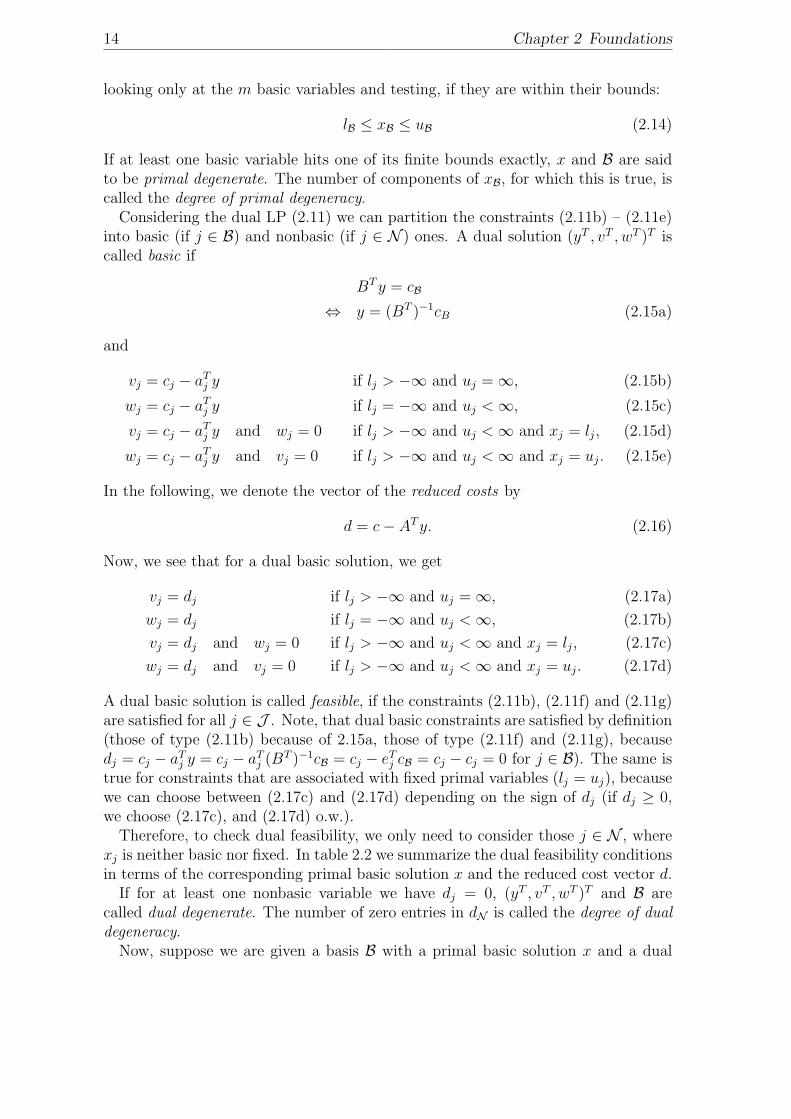
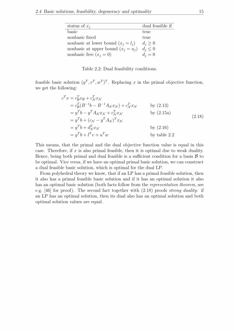
Therefore, to check dual feasibility, we only need to consider those j ∈ N , wherexj is neither basic nor fixed. In table 2.2 we summarize the dual feasibility conditionsin terms of the corresponding primal basic solution x and the reduced cost vector d.
If for at least one nonbasic variable we have dj = 0, (yT , vT , wT )T and B arecalled dual degenerate. The number of zero entries in dN is called the degree of dualdegeneracy.
Now, suppose we are given a basis B with a primal basic solution x and a dual
2.4 Basic solutions, feasibility, degeneracy and optimality 15
status of xj dual feasible ifbasic truenonbasic fixed truenonbasic at lower bound (xj = lj) dj ≥ 0nonbasic at upper bound (xj = uj) dj ≤ 0nonbasic free (xj = 0) dj = 0
Table 2.2: Dual feasibility conditions.
feasible basic solution (yT , vT , wT )T . Replacing x in the primal objective function,we get the following:
cTx = cTBxB + cTNxN
= cTB(B−1b−B−1ANxN ) + cTNxN by (2.13)
= yT b− yTANxN + cTNxN by (2.15a)
= yT b+ (cN − yTAN )TxN
= yT b+ dTNxN by (2.16)
= yT b+ lTv + uTw by table 2.2
(2.18)
This means, that the primal and the dual objective function value is equal in thiscase. Therefore, if x is also primal feasible, then it is optimal due to weak duality.Hence, being both primal and dual feasible is a sufficient condition for a basis B tobe optimal. Vice versa, if we have an optimal primal basic solution, we can constructa dual feasible basic solution, which is optimal for the dual LP.
From polyhedral theory we know, that if an LP has a primal feasible solution, thenit also has a primal feasible basic solution and if it has an optimal solution it alsohas an optimal basic solution (both facts follow from the representation theorem, seee.g. [46] for proof). The second fact together with (2.18) proofs strong duality : ifan LP has an optimal solution, then its dual also has an optimal solution and bothoptimal solution values are equal.

16 Chapter 2 Foundations
17
Chapter 3
The Dual Simplex Method
3.1 The Revised Dual Simplex Algorithm
3.1.1 Basic idea
Simplex type algorithms search the space of basic solutions in a greedy way, untileither infeasibility or unboundedness is detected or an optimal basic solution is found.While the primal simplex algorithm maintains primal feasibility and stops when dualfeasibility is established, the dual simplex algorithm starts with a dual feasible basisand works towards primal feasibility.
Algorithm 1: Basic steps of the dual simplex method.
Input: LP in computational form (2.2), dual feasible basis BOutput: Optimal basis B or proof that LP is dual unbounded.
Pricing(Step 1)Find a leaving variable p ∈ B, that is primal infeasible. If no such pexists, then B is optimal → exit.
Ratio Test(Step 2)Find an entering variable q ∈ N , such (B \ p) ∪ q is a again dualfeasible basis. If no such q exists, then the LP is dual unbounded →exit.
Basis change(Step 3)Set B ← (B \ p) ∪ q and N ← (N \ q) ∪ p.Update problem data.
Go to step 1.
Algorithm 1 shows the basic steps of the dual simplex method. In each iterationit moves from the current dual feasible basis to a neighboring basis by exchanginga variable in B by a variable in N . Since we want to reduce primal infeasibility,a primal infeasible basic variable is chosen to leave the basis in step 1 and is madenonbasic (hence, primal feasible) by setting it to one of its finite bounds (free variablesare not eligible here). In section 3.1.3 we will see, that this selection also ensures anondecreasing dual objective function value. If no primal infeasible variable exist, we
18 Chapter 3 The Dual Simplex Method
know, that the current basis must be optimal, because it is primal and dual feasible.In step 1 a nonbasic variable is selected to enter the basis, such that the new basis isagain dual feasible. We will see in section 3.1.4, that the LP is dual unbounded (i.e.primal infeasible), if no entering variable can be determined. Finally, all necessaryupdate operations associated with the basis change are carried out in step 1.
To be able to apply algorithm 1 to some given LP we are left with the task toobtain a dual feasible basis to start with. There are a variety of methods to do this,which we will discuss in chapter 4. At first, we will describe in greater detail whatwe mean by neighboring solution, dual pricing, ratio test and basis change.
3.1.2 Neighboring solutions
Let B = {k1, . . . , km} be a dual feasible basis, (yT , vT , wT )T a corresponding dualfeasible basic solution and x a corresponding primal basic solution. In this situationwe know, that the dual constraints (2.11c) – (2.11e) hold at equality for all j ∈ B(we do not consider constraint (2.11b) here, because free variables are not eligible toleave the basis) and that the corresponding dual logical variables are equal to zero. Ifvariable p = B(r) leaves the bases, then the r-th dual basic constraint may (but neednot) change from equality to inequality, while all other dual constraints associatedwith basic variables keep holding at equality. Denoting the new dual solution by(yT , vT , wT )T and the change in the r-th dual basic constraint by t ∈ R, such that
t = aTp y − aT
p y (3.1)
we get
aTp y − t = aT
p y (3.2a)
and
aTj y = aT
j y for all j ∈ B \ {p}, (3.2b)
which can be written concisely as
BT y − er t = BTy. (3.3)
From equation 3.3 we get
y = y + (BT )−1er t
= y + ρrt, (3.4)
where ρr = (BT )−1er denotes the r-th column of (BT )−1, as an update formula fory and
d = c− AT y
3.1 The Revised Dual Simplex Algorithm 19
= c− AT (y + ρrt)
= d− AT (BT )−1er t
= d− αr t, (3.5)
where αr = eTr B
−1A denotes the r-th row of the transformed constraint matrixB−1A, as an update formula for d.
Obviously, αrj = eT
r B−1aj = eT
r ej = 0 for all j ∈ B \ {p} and αrp = eT
r B−1ap =
eTr er = 1. Hence, (3.5) can be stated more precisely as
dj = dj = 0 for all j ∈ B \ {p}, (3.6a)
dp = −t and (3.6b)
dj = dj − αrj t for all j ∈ N . (3.6c)
The change in the r-th dual basic constraint has to be compensated by the corre-sponding dual logical variable(s). We say, that the constraint is relaxed in a feasibledirection, if the dual logicals stay feasible. If it is a constraint of type (2.11c), we getvp = −t, hence we need t ≤ 0. If it is a constraint of type (2.11d), we get wp = −t,hence we need t ≥ 0. If it is a constraint of type (2.11e), both directions are feasible:we set vp = −t, wp = 0 if t ≤ 0 and vp = 0, wp = −t if t ≥ 0.
In the next two sections, we will clarify, how to choose p and t, such that the dualobjective function improves and (yT , vT , wT )T is again a dual feasible basic solution.
3.1.3 Pricing
If we relax a dual basic constraint p in a dual feasible direction with the restriction,that no dj with j ∈ N changes sign (or leaves zero), we get the following dualobjective function value Z for the new dual solution (yT , vT , wT )T :
Z = bT y +∑j ∈J
lj>−∞
lj vj +∑j ∈Juj<∞
ujwj
= bT y +∑j ∈Ndj ≥ 0
lj dj +∑j ∈Ndj ≤ 0
uj dj − tu±p , where u±
p =
{lp if t ≤ 0
up if t ≥ 0
= bT (y + teTr B
−1) +∑j ∈Ndj ≥ 0
lj(dj − teTr B
−1aj) +∑j ∈Ndj ≤ 0
uj(dj − teTr B
−1aj)− tu±p
= Z + teTr B
−1b−∑j ∈Ndj ≥ 0
teTr B
−1ajlj −∑j ∈Ndj ≤ 0
teTr B
−1ajuj − tu±p
= Z + teTr B
−1(b− ANxN )− tu±p
= Z + teTr xB − tu±
p
= Z + t(xp − u±p )
20 Chapter 3 The Dual Simplex Method
= Z + ∆Z, where ∆Z =
{t(xp − lp) if t ≤ 0
t(xp − up) if t ≥ 0.(3.7)
Now we can determine p and the sign of t such that ∆Z is positive, since we wantthe dual objective function to increase (maximization). We select p such that eitherxp < lp and t ≤ 0 or xp > up and t ≥ 0. In both cases the leaving variable can beset to a finite bound, such that it does not violate the dual feasibility conditions. Ift ≤ 0, xp = lp is dual feasible, since dp = −t ≥ 0. The same is true for the caset ≥ 0: xp = up is dual feasible, since dp = −t ≤ 0. In the next section we will see,how dual feasibility is maintained for the remaining nonbasic variables.
Note, that xp is eligible to leave the basis only if it is primal infeasible. If there isno primal infeasible basic variable left, no further improvement in the dual objectivefunction can be accomplished. The decision which of the primal infeasible variablesto select as leaving variable has great impact on the number of total iterations of themethod. As in the primal simplex method, simple rules (like choosing the variablewith the greatest infeasibility) have turned out to be inefficient for the dual simplexalgorithm. We will discuss suitable pricing rules in section 3.3. In section 8.2.2 wewill describe further computational aspects that have to be taken into account foran efficient implementation of the pricing step.
3.1.4 Ratio test
In the previous section we saw that the dual logical of the relaxed basic constraintalways remains dual feasible. Since all other basic constraints stay at equality, weonly have to consider the nonbasic dual logicals to fulfill the dual feasibility conditions(see table 2.2). Furthermore, we can neglect dual logicals that are associated withfixed primal variables because they can never go dual infeasible.
As t moves away from zero, we know, that the nonbasic dual logicals evolve ac-cording to equation (3.6c):
dj = dj − αrj t for all j ∈ N (3.8)
If xj = lj, dual feasibility is preserved as long as
dj ≥ 0
⇔ dj − αrjt ≥ 0
⇔ t ≥ dj
αrj
if αrj < 0 and t ≤ dj
αrj
if αrj > 0.
(3.9)
If xj = uj, dual feasibility is preserved as long as
dj ≤ 0
⇔ dj − αrjt ≤ 0
⇔ t ≥ dj
αrj
if αrj > 0 and t ≤ dj
αrj
if αrj < 0.
(3.10)
If xj is free, dual feasibility is preserved as long as
3.1 The Revised Dual Simplex Algorithm 21
dj = 0
⇔ dj − αrjt = 0
⇔ t =dj
αrj
= 0 since dj = 0.
(3.11)
When a nonbasic constraint j becomes tight (i.e. dj = 0), it gets eligible to replacethe relaxed constraint p in the set of basic constraints. The constraints that becometight first as t is increased (or decreased) define a bound θD on t, such that dualfeasibility is not violated. Among them, we select a constraint q to enter the basis.The associated primal variable xq is called entering variable and θD is called dual steplength. We call a value of t, at which a constraint becomes tight, a breakpoint. If noconstraint becomes tight, no breakpoint exists and the problem is dual unbounded.
If t ≥ 0 is required, we can denote the set of subscripts, which are associated withpositive breakpoints, by
F+ = {j : j ∈ N , xj free or(xj = lj and αrj > 0) or (xj = uj and αr
j < 0)}. (3.12)
If F+ = ∅, then there exists no bound on t and the problem is dual unbounded.Otherwise, q and θD are determined1 by
q ∈ arg minj∈F+
{dj
αrj
}and θD =
dq
αqj
. (3.13)
If t ≤ 0 is required, we can denote the set of subscripts, which are associated withbreakpoints, by
F− = {j : j ∈ N , xj free or(xj = lj and αrj < 0) or (xj = uj and αr
j > 0)}. (3.14)
As above, if F− = ∅, the problem is dual unbounded. Otherwise, q and θD aredetermined2 by
q ∈ arg maxj∈F−
{dj
αrj
}and θD =
dq
αqj
. (3.15)
To ease the algorithmic flow we can get rid of the negative case (t ≤ 0) by settingαr
j = αrj if t ≥ 0 and αr
j = −αrj if t ≤ 0. Then, we can use only equations (3.12) and
(3.13) with α instead of α to determine q and θD (see step 2 in algorithm 2).Note, that there can be more then one choice for q in (3.13) and (3.15), since there
might be several breakpoints with the same minimal (or maximal) value. This is thecase for example, if the current basis is dual degenerate by a degree greater than one(more than one nonbasic dj is zero). In that situation, we can choose the one amongthem, that has favorable computational properties. If free nonbasic variables exist,then the basis must be dual degenerate. Therefore, they are always eligible to enter
1In the absence of degeneracy the minimum in equation 3.13 is unique.2In the absence of degeneracy the maximum in equation 3.15 is unique.
22 Chapter 3 The Dual Simplex Method
the basis right away.
3.1.5 Basis change
In the pricing step and the dual ratio test we have determined a variable that entersand one that leaves the basis. In the basis change step we update all the vectors whichare required to start the next iteration with the new basis, i.e., the dual basic solution,the primal basic solution, the objective function value and the representation of thebasis (and its inverse).
As we have seen before, the dual logicals v and w coincide with the reduced costvector d. Therefore, the dual basic solution can be represented by (yT , dT )T . Insection 3.1.2 we have already derived update formulae for y and d. Using the dualstep length θD for t, we get
y = y + θDρr, where ρr = (BT )−1er, (3.16a)
for y and
dp = −θD, (3.16b)
dq = 0, (3.16c)
dj = dj = 0 for all j ∈ B \ {p} (3.16d)
dj = dj − θDαrj for all j ∈ N \ {q} (3.16e)
for d. Note, that it is not necessary though to update both vectors y and d. In mostpresentations of the dual simplex method (as in ours so far), only an update of dis needed. We can as well formulate a version of the algorithm, in which only y isupdated. In this case, those entries of dN , which are needed for the ratio test, mustbe computed in place from their definition.
Considering the primal basic solution x, we know that the leaving variable xp
goes to one of its finite bounds and that the variable xq might leave its bound whileentering the basis. The displacement of xq is denoted by θP and called primal steplength. Hence, we get for the primal variables in N ∪ {p}:
xp =
{lp if xp < lp
up if xp > up,(3.17a)
xq = xq + θP and (3.17b)
xj = xj for all j ∈ N \ {q} (3.17c)
Let j = B(i) and ρi = (BT )−1ei. Then we can derive an update formula for basicprimal variables j ∈ B \ {p} from equation (2.13):
xj = ρi(b− AN xN )
3.1 The Revised Dual Simplex Algorithm 23
= ρib− αiN xN
= ρib−∑
j∈N\{q}
αijxj − αi
q(xq + θP )
= xj − θPαiq (3.17d)
Finally, we can compute the primal step length θP by using (3.17d) for xp:
xp = xp − θPαpq
⇔ θP =xp − lpαp
qif xp < lp or θP =
xp − up
αpq
if xp > up.(3.18)
To represent the basis and its inverse in a suitable form is one of the most importantcomputational aspects of the (dual) simplex method. We will leave the computa-tional techniques which are used to maintain these representations and to solve therequired systems of linear equations for chapter 5. For now, we will only investigatehow the basic submatrix B and its inverse alter in a basis change. We start byrestating the obvious update of the index sets B and N (which in a computationalcontext are called basis heading):
B = (B \ p) ∪ qN = (N \ q) ∪ p.
(3.19)
The new basis matrix B emerges from the old basis matrix B by substituting itsr-th column by the entering column aq, where p = B(r):
B = B −BereTr + aqe
Tr
= B + (aq −Ber) eTr
= B(I +B−1 (aq −Ber) e
Tr
)= B
(I + (αq − er) e
Tr
), (3.20)
where αq = B−1aq. Let F be defined as
F = I + (αq − er) eTr . (3.21)
Hence, F corresponds to an identity matrix, where the r-th column is replaced byαq:
F =
1 α1
q. . .
...αr
q...
. . .
αmq 1
. (3.22)
With equations (3.20) and (3.21) the basis matrix B can be displayed as follows:
24 Chapter 3 The Dual Simplex Method
B = BF. (3.23)
Let E = F−1, then we get for B−1:
B−1 = EB−1. (3.24)
The inverse of the new basis matrix is the result of the old basis inverse multipliedwith matrix E. It is easy to verify that E exists if and only if αr
q 6= 0 and then hasthe form
E =
1 η1
. . ....ηr...
. . .
ηm 1
, (3.25)
where
ηr =1
αrq
and ηi = −αi
q
αrq
for i = 1, . . . ,m, i 6= r. (3.26)
A matrix of this type is called an elementary transformation matrix (ETM) or short:eta-matrix. Let ρi, i = 1, . . . ,m, be the rows of B−1. Then, we get from equa-tion (3.24) and the entries of η in (3.26) for the rows ρi of B−1:
ρr =1
αrq
ρr and (3.27)
ρi = ρi −αi
q
αrq
ρr for i = 1, . . . ,m, i 6= r. (3.28)
Equation 3.24 is the basis for the so called PFI update (where PFI stands for productform of the inverse). The idea is to represent the basis inverse as a product ofeta-matrices in order to efficiently solve the linear systems efficiently required inthe simplex method. This can be done by initializing the solution vector by theright-hand-side of the system and the successively multiply it with the eta-matrices.Depending on wether the system consists of the basis matrix or the transpose of thebasis matrix this procedure is performed from head to tail (called forward transition –FTran) of the eta-sequence or from tail to head (called backward transition – BTran),respectively. The sequence of eta-matrices can be stored in a very compact way sinceonly the nonzero elements in the r-column have to be remembered. However, thePFI-update was replaced by the so called LU-update, which turned out to allow foran even sparser representation and also proved to be numerically more stable. LUfactorization and update techniques will be described in great detail in chapter 5.
3.2 The Bound Flipping Ratio Test 25
3.1.6 Algorithmic descriptions
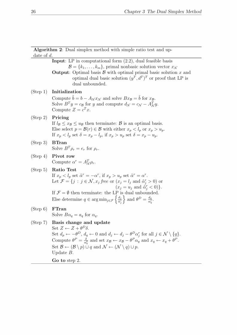
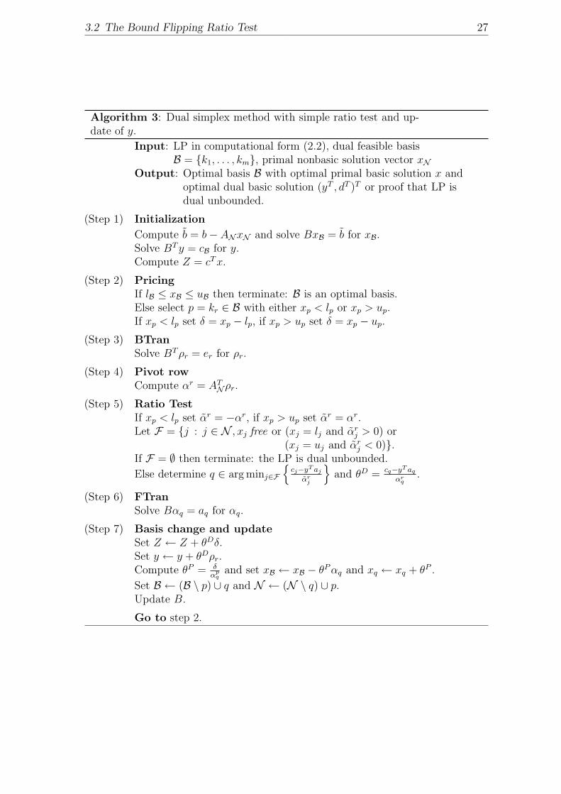
The revised dual simplex method with simple ratio test and update of d is sum-marized in algorithm 2. Algorithm 3 is a variant where y is updated instead of d.Although the first version seems to be clearly more efficient on the first sight, thesituation actually depends on sparsity characteristics of the problem instance andthe implementation of the steps Pivot Row and Ratio Test.
3.2 The Bound Flipping Ratio Test
The simple dual ratio test described in section 3.1.4 selects the entering index qamong those nonbasic positions that would become dual infeasible if the displacementt of the r-th dual basic constraint was further increased (or decreased resp.). Thebound flipping ratio test (which is sometimes also called generalized ratio test or longstep rule) is based on the observation, that a boxed nonbasic variable xj can bekept dual feasible even if its reduced cost value dj switches sign by setting it to itsopposite bound (see table 2.2). This means, that we may further increase the dualstep length and pass by breakpoints in the ratio test which are associated with boxedprimal variables as long as the dual objective function keeps improving. It can beseen that the rate of improvement decreases with every bound flip. When it dropsbelow zero no further improvement can be made and the entering variable can beselected from the current set of bounding breakpoints (all of which have the samevalue).
According to Kostina [41] the basic idea of the bound flipping ratio test has beenfirst published in the Russian OR community by Gabasov, Kirillova and Kostyukova [57]as early as 1979. In western OR literature mostly Fourer [27] is cited to be the firstone to publish it. In our description we follow Fourer and Maros [47].
To describe the bound flipping ratio test precisely let us consider the case wherexp > up and t > 0. In equation (3.7) we see, that the slope of the dual objectivefunction with respect to t is given by
δ1 = xp − up (3.29)
as long as no dj changes sign, i.e,
0 ≤ t ≤ θD1 with q1 ∈ arg min
j∈Q+1
{dj
αrj
}, θD
1 =dq1
αrq1
and Q+1 = F+. (3.30)
For t = θD1 we have dq1 = dq1 − tαr
q1= 0 and q1 is eligible to enter the basis. The
change ∆Z1 of the dual objective function up to this point is
∆Z1 = θD1 δ
D1 . (3.31)
If t is further increased, such that t > θD1 , then we get two cases dependent on the
sign of αrq1
.
• If αq1 > 0, then dq1 becomes negative and goes dual infeasible since in this
26 Chapter 3 The Dual Simplex Method
Algorithm 2: Dual simplex method with simple ratio test and up-date of d.
Input: LP in computational form (2.2), dual feasible basisB = {k1, . . . , km}, primal nonbasic solution vector xN
Output: Optimal basis B with optimal primal basic solution x andoptimal dual basic solution (yT , dT )T or proof that LP isdual unbounded.
Initialization(Step 1)
Compute b = b− ANxN and solve BxB = b for xB.Solve BTy = cB for y and compute dN = cN − AT
Ny.Compute Z = cTx.
Pricing(Step 2)If lB ≤ xB ≤ uB then terminate: B is an optimal basis.Else select p = B(r) ∈ B with either xp < lp or xp > up.If xp < lp set δ = xp − lp, if xp > up set δ = xp − up.
BTran(Step 3)Solve BTρr = er for ρr.
Pivot row(Step 4)Compute αr = AT
Nρr.
Ratio Test(Step 5)If xp < lp set αr = −αr, if xp > up set αr = αr.Let F = {j : j ∈ N , xj free or (xj = lj and αr
j > 0) or(xj = uj and αr
j < 0)}.If F = ∅ then terminate: the LP is dual unbounded.
Else determine q ∈ arg minj∈F
{dj
αrj
}and θD = dq
αrq.
FTran(Step 6)Solve Bαq = aq for αq.
Basis change and update(Step 7)Set Z ← Z + θDδ.Set dp ← −θD, dq ← 0 and dj ← dj − θDαr
j for all j ∈ N \ {q}.Compute θP = δ
αpq
and set xB ← xB − θPαq and xq ← xq + θP .
Set B ← (B \ p) ∪ q and N ← (N \ q) ∪ p.Update B.
Go to step 2.
3.2 The Bound Flipping Ratio Test 27
Algorithm 3: Dual simplex method with simple ratio test and up-date of y.
Input: LP in computational form (2.2), dual feasible basisB = {k1, . . . , km}, primal nonbasic solution vector xN
Output: Optimal basis B with optimal primal basic solution x andoptimal dual basic solution (yT , dT )T or proof that LP isdual unbounded.
Initialization(Step 1)
Compute b = b− ANxN and solve BxB = b for xB.Solve BTy = cB for y.Compute Z = cTx.
Pricing(Step 2)If lB ≤ xB ≤ uB then terminate: B is an optimal basis.Else select p = kr ∈ B with either xp < lp or xp > up.If xp < lp set δ = xp − lp, if xp > up set δ = xp − up.
BTran(Step 3)Solve BTρr = er for ρr.
Pivot row(Step 4)Compute αr = AT
Nρr.
Ratio Test(Step 5)If xp < lp set αr = −αr, if xp > up set αr = αr.Let F = {j : j ∈ N , xj free or (xj = lj and αr
j > 0) or(xj = uj and αr
j < 0)}.If F = ∅ then terminate: the LP is dual unbounded.
Else determine q ∈ arg minj∈F
{cj−yT aj
αrj
}and θD = cq−yT aq
αrq
.
FTran(Step 6)Solve Bαq = aq for αq.
Basis change and update(Step 7)Set Z ← Z + θDδ.Set y ← y + θDρr.Compute θP = δ
αpq
and set xB ← xB − θPαq and xq ← xq + θP .
Set B ← (B \ p) ∪ q and N ← (N \ q) ∪ p.Update B.
Go to step 2.
28 Chapter 3 The Dual Simplex Method
case xq1 = lq1 (otherwise q1 would not define a breakpoint). If xq1 is a boxedvariable though, it can be kept dual feasible by setting it to uq1 .
• If αq1 < 0, then dq1 becomes positive and goes dual infeasible since in thiscase xq1 = uq1 (otherwise q1 would not define a breakpoint). If xq1 is a boxedvariable though, it can be kept dual feasible by setting it to lq1 .
Since a bound flip of a nonbasic primal variable xq1 effects the values of the primalbasic variables and especially xp, also the slope of the dual objective function changes.For xB we have
xB = B−1(b− ANxN )
= B−1b−B−1ANxN
= B−1b−∑j∈N
(B−1aj)xj
= B−1b−∑j∈N
αjxj. (3.32)
Consequently, if αq1 > 0 and xq1 is set from lq1 to uq1 , xp changes by an amount of−αr
q1uq1 + αr
q1lq1 and we get for the slope beyond δD
1 :
δ2 = xp − αrq1uq1 + αr
q1lq1 − up
= xp − (uq1 − lq1)αrq1− up
= δ1 − (uq1 − lq1)αrq1. (3.33)
If αq1 < 0 and xq1 is set from uq1 to lq1 , xp changes by an amount of αrq1uq1 − αr
q1lq1
and we get for the slope beyond δD1 :
δ2 = xp + αrq1uq1 − αr
q1lq1 − up
= xp + (uq1 − lq1)αrq1− up
= δ1 + (uq1 − lq1)αrq1. (3.34)
Hence, in both cases the slope decreases by (uq1− lq1)|αrq1|. If the new slope δ2 is still
positive, it is worthwhile to increase t beyond θD1 , until the next breakpoint θD
2 with
θD2 =
dq2
αrq2
with q2 ∈ arg minj∈Q+
2
{dj
αrj
}and Q+
2 = Q+1 \ {q1}. (3.35)
is reached. The change of the dual objective function as t moves from θD1 to θD
2 is
∆Z2 = (θD2 − θD
1 )δ2. (3.36)
This procedure can be iterated until either the slope becomes negative or dual un-boundedness is detected in iteration i if Q+
i = ∅. In the framework of the dualsimplex algorithm these iterations are sometimes called mini iterations. As in thesimple ratio test the case for t < 0 is symmetric and can be transformed to the case
3.2 The Bound Flipping Ratio Test 29
t > 0 by switching the sign of αr. Only the slope has to be initialized differently bysetting δ1 = |xp − lp|.
One of the features of the BFRT is, that under certain conditions it is possible toperform an improving basis change even if the current basis is dual degenerate. Tosee this, suppose that the first k breakpoints θD
i , i = 1, . . . , k are zero (hence, dqi= 0
for i = 1, . . . , k) and θDk+1 > 0. Then the eventual step length θD = dq/α
rq can be
strictly positive if and only if after k mini iterations the slope δk is still positive, i.e.
δk = δ1 −k∑
i=1
(uqi− lqi
)|αrqi| > 0 (3.37)
Obviously, it depends on the magnitude of the initial primal infeasibility δ1 andthe respective entries in the pivot row αr
qias well as on the distances between the
individual bounds wether or not this condition can be met. It turns out however, thatespecially on the LP-relaxations of combinatorial optimization problems, which areoften highly degenerate, the BFRT works very well. This is why the implementationof the BFRT is particularly important in dual simplex codes, which are supposed tobe integrated into a branch-and-bound based MIP-code like MOPS.
When an entering variable q = qk has eventually been determined after k iterations,we have to update the primal basic variables xB according to the bound flips inxN . Let T = {q1, . . . , qk} be the set of indices of all of the nonbasic variables,which are to be set to their opposite bound, T + = {j ∈ T |αr
j > 0} the set ofindices of those nonbasic variables, which switch from lower to upper bound andT − = {j ∈ T |αr
j < 0} the set of indices of those nonbasic variables, which switchfrom upper to lower bound. Then, according to equation 3.32, xB can be updatedin the following way:
xB = xB −∑j∈T +
(uj − lj)αj −∑j∈T −
(lj − uj)αj
= xB −B−1
∑j∈T +
(uj − lj)aj +∑j∈T −
(lj − uj)aj
= xB −∆xB, (3.38)
where ∆xB is the solution vector of the linear system
B∆xB = a with a =∑j∈T +
(uj − lj)aj +∑j∈T −
(lj − uj)aj. (3.39)
There are different ways to embed the bound flipping ratio test into the reviseddual simplex method given in the form of algorithm 2. In both Fourer’s and Maros’description the selection of the leaving variable and the update operations for xB andZ are integrated in the sense, that the sets T + and T − as well as the summationof a are done in the main selection loop for q. We will present a version that ismotivated by the dual simplex implementation in the COIN LP code [44], where theupdate operations are strictly separated from the selection of the entering variable.
30 Chapter 3 The Dual Simplex Method
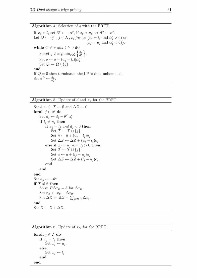
Even the bound flips are not recorded in the ratio test but during the update of thereduced cost vector d. If an updated entry dj is detected to be dual infeasible, thecorresponding nonbasic primal variable (which must be boxed in this case) is markedfor a bound flip and column aj is added to a. After the update of d, system (3.39)is solved and xB is updated according to (3.38). The actual bound flips in xN areonly performed at the very end of a major iteration.
The three parts selection of the entering variable, update of d and xB and updateof xN are described in algorithms 4, 5 and 6 respectively. The update of the objectivefunction value can be done in two different ways. One way is to compute the objectivechange in the selection loop for q in algorithm 4 by an operation of type (3.36). Theother way is to look at the objective function value from a primal perspective. Fromequation (2.18) we know, that in every iteration of the dual simplex method theprimal and the dual objective function value is equal for the current primal and dualsolution (provided that v and w are set according to equation (2.17)):
cTBxB + cTNxN = bTy + lTv + uTw. (3.40)
Hence, we can as well compute the change in the objective function value by takinginto account the change of the primal basic and nonbasic variables caused by thebound flips:
∆Z = −∑j∈B
cj∆xj +∑j∈T +
cj(uj − lj) +∑j∈T +
cj(uj − lj). (3.41)
Thus, also this update operation can be separated from the selection loop for q andmoved to algorithm 5.
3.3 Dual steepest edge pricing
In the pricing step of the dual simplex method we have to select a variable to leavethe basis among all of those variables which are primal infeasible. In geometricalterms, this corresponds to choosing a search direction along one of the edges of thedual polyhedron emanating from the vertex defined by the current basic solution,which makes an acute3 angle with the gradient of the dual objective function. Thebasic idea of dual steepest edge pricing (DSE) is to determine the edge direction thatforms the most acute angle with the dual gradient and is in this sense steepest.
We will follow the description of Forrest and Goldfarb [26], who described thefirst practical steepest edge variants for the dual simplex method. Surprisingly, theyshowed in numerical experiments, that their simplest version, which they call Dualalgorithm I performs best in most cases.
This variant of DSE is derived for a problem in computational standard form (2.5).
3since we are maximizing
3.3 Dual steepest edge pricing 31
Algorithm 4: Selection of q with the BRFT.
If xp < lp set αr ← −αr, if xp > up set αr ← αr.Let Q ← {j : j ∈ N , xj free or (xj = lj and αr
j > 0) or(xj = uj and αr
j < 0)}.while Q 6= ∅ and δ ≥ 0 do
Select q ∈ arg minj∈Q
{dj
αrj
}.
Set δ ← δ − (uq − lq)|αrq|.
Set Q ← Q \ {q}.endIf Q = ∅ then terminate: the LP is dual unbounded.Set θD ← dq
αrq.
Algorithm 5: Update of d and xB for the BRFT.
Set a← 0, T ← ∅ and ∆Z ← 0.forall j ∈ N do
Set dj ← dj − θDαrj .
if lj 6= uj thenif xj = lj and dj < 0 then
Set T ← T ∪ {j}.Set a← a+ (uj − lj)aj.Set ∆Z ← ∆Z + (uj − lj)cj.
else if xj = uj and dj > 0 thenSet T ← T ∪ {j}.Set a← a+ (lj − uj)aj.Set ∆Z ← ∆Z + (lj − uj)cj.
end
end
endSet dp ← −θD.if T 6= ∅ then
Solve B∆xB = a for ∆xB.Set xB ← xB −∆xB.Set ∆Z ← ∆Z −
∑j∈B cj∆xj.
endSet Z ← Z + ∆Z.
Algorithm 6: Update of xN for the BRFT.
forall j ∈ T doif xj = lj then
Set xj ← uj.else
Set xj ← lj.end
end
32 Chapter 3 The Dual Simplex Method
The dual of (2.5) reads:
Z∗ = max bTy (3.42a)
s.t. ATy ≤ c. (3.42b)
Given a basis B a dual solution y is basic for problem (3.42), if BTy = cB andfeasible, if AT
Ny ≤ cN . If the i-th tight basic constraint j ∈ B is relaxed, such thataT
j y + t = cj, i.e., aTj y ≤ cj for t ≥ 0, then all other basic constraint stay tight, if
BT y + tei = cB, which leads to y = y − tρi with ρi = B−T ei. Hence, −ρi is the edgedirection associated with the i-th potential basic leaving variable.
Obviously, the gradient of the dual objective function (3.42a) is b. The angle γbetween b and −ρi is acute, if −ρT
i b = −eTi B
−1b = −eTi xB = −xB(i) is positive (xB(i)
primal infeasible with xB(i) ≤ 0). Furthermore, we have
− xB(i) = −bTρi = ‖b‖‖ρi‖ cos γ, (3.43)
where ‖ · ‖ is the Euclidian norm. Since ‖b‖ is constant for all edge directions, wecan determine the leaving variable p = B(r) with the steepest direction by
r ∈ arg maxi∈{1,...,m}
{−xB(i)
‖ρi‖: xB(i) < 0
}. (3.44)
To compute the norms ‖ρi‖ from their definition would require the solution of upto m systems of linear equations (one for each vector ρi) and just as many innerproducts. The actual accomplishment of Forrest and Goldfarb is the presentation ofexact update formulas for the squares of these norms, which we will denote by
βi = ρTi ρi = ‖ρi‖2. (3.45)
The values βi are called dual steepest edge weights. Using the weights instead of thenorms is straightforward, the selection rule (3.44) just has to be modified as follows:
r ∈ arg maxi∈{1,...,m}
{(xB(i))
2
βi
: xB(i) < 0
}. (3.46)
From the update formulas (3.27) for the ρi we can conclude, that the DSE weightsβi after the basis change are
βr = ρTr ρr =
(1
αrq
)2
βr (3.47a)
and
βi = ρTi ρi
=
(ρT
i −αi
q
αrq
ρTr
)(ρi −
αiq
αrq
ρr
)
3.3 Dual steepest edge pricing 33
= βi − 2αi
q
αrq
ρTr ρi +
(αi
q
αrq
)2
βr for i = 1, . . . ,m, i 6= p. (3.47b)
Since we do not want to calculate all the ρi explicitly during a dual iteration, it isnot obvious, how to efficiently compute the term ρT
r ρi. Fortunately, we can write
ρTr ρi = ρT
i ρr = eTi B
−1ρr = eTi τ = τi, (3.48)
where τ = B−1ρr. Hence, it suffices to solve only one additional linear system for τ :
Bτ = ρr. (3.49)
Due to (3.48) equation (3.47b) can be rewritten as
βi = βi − 2αi
q
αrq
τi +
(αi
q
αrq
)2
βr. (3.50)
Note that numerical stability can be improved at small additional computationalcosts by computing βr explicitly, since ρr is available from the computation of thetransformed pivot row (see step 2 in algorithm 2).
Besides the geometrical motivation of DSE pricing it can also be viewed as astrategy to reduce or even eliminate misleading scaling effects when using the simpleDantzig pricing rule. To make this clear, suppose the columns of A are scaled bynumbers 1
sj> 0, such that aj = 1
sjaj. Since ρiaB(i) = 1, this leads to scaled vectors
ρi = sB(i)ρi and hence, to scaled primal basic variables xB(i) = ρib = sB(i)ρib =sB(i)xB(i). Consequently, the magnitude of the primal infeasibilities totally dependson the (problem inherent) column scales, which may result in a suboptimal pricingdecision by the Dantzig rule. However, dividing the primal basic variables by the Eu-clidian norms ‖ρi‖ yields primal infeasibilities which are independent of the columnscales:
xB(i) =xB(i)
‖ρi‖=sB(i)xB(i)
‖sB(i)ρi‖=xB(i)
‖ρi‖. (3.51)
In the case of the general computational form (2.2) and its dual (2.11) the edgedirections need to be extended by additional components for v and w. This leadsto computationally more expensive update formulas for the DSE weights (see [26]).In fact, in this case one more linear system and an inner product have to be solved.It has been shown that for most problems this additional effort does not pay off,i.e., it is not compensated by the additional reduction in the total number of itera-tions. Therefore, we keep using the DSE weights from above to normalize the primalinfeasibilities even if upper and lower bounds are present. Denoting the primal in-feasibilities by
δi =
xB(i) − lB(i) if xB(i) < lB(i)
xB(i) − uB(i) if xB(i) > uB(i)
0 o.w.
(3.52)
34 Chapter 3 The Dual Simplex Method
the leaving variable is selected by
r ∈ arg maxi∈{1,...,m}
{|δi|2
βi
: δi 6= 0
}. (3.53)
This turns the method into a heuristic in the sense, that we cannot guarantee any-more that always the leaving variable associated with the steepest edge directionis chosen. The efficiency and actual performance of DSE pricing depends heavilyon implementation details. We give a detailed description of our DSE code in sec-tion 8.2.2.
3.4 Elaborated version of the Dual Simplex Algorithm
Algorithm 7 shows a complete mathematical description of the dual simplex methodas it is implemented in MOPS. It can be seen as a variant of algorithm 2 enhanced bysteepest pricing (described in section 3.3) and the bound flipping ratio test (describedin section 3.2).
Note, that in this version of the method, up to four systems of linear equationshave to be solved in every iteration:
• BTρr = er in step 7 to compute the transformed pivot row αr = ρTr AN , which
is needed in the ratio test,
• Bαq = aq in step 7 to compute the transformed pivot column αq, which isneeded to update xB and B,
• Bτ = ρr in step 7 to update the steepest edge weights and
• B∆xB = a in algorithm 5 to update the primal basic variable if bound flipshave to be performed.
Besides the computation of the transformed pivot row in step 7 these are the mosttime consuming operations for a great majority of problems. In chapter 5 we willdescribe the computational techniques that are deployed to perform them efficiently.
Furthermore, algorithm 7 can only be applied if we have a dual feasible basicsolution to start with. If the default starting basis (usually consisting of the identitymatrix I associated with the logical variables) is not dual feasible we have to proceedin two phases. In the first phase, we try to obtain a dual feasible basis by so calleddual phase I methods. A possible outcome of these methods is that no dual feasiblesolution exists for the given LP problem and we have to terminate (or try to furtheranalyse, wether the problem is also primal infeasible or primal unbounded). If phaseI succeeds in obtaining a dual feasible basis we call algorithm 7 as a second phase toprove optimality or dual unboundedness. In this sense, we will call algorithm 7 dualphase II. In the following chapter 4 we will describe several dual phase I methods,which we will evaluate and compare computationally in chapter 9.
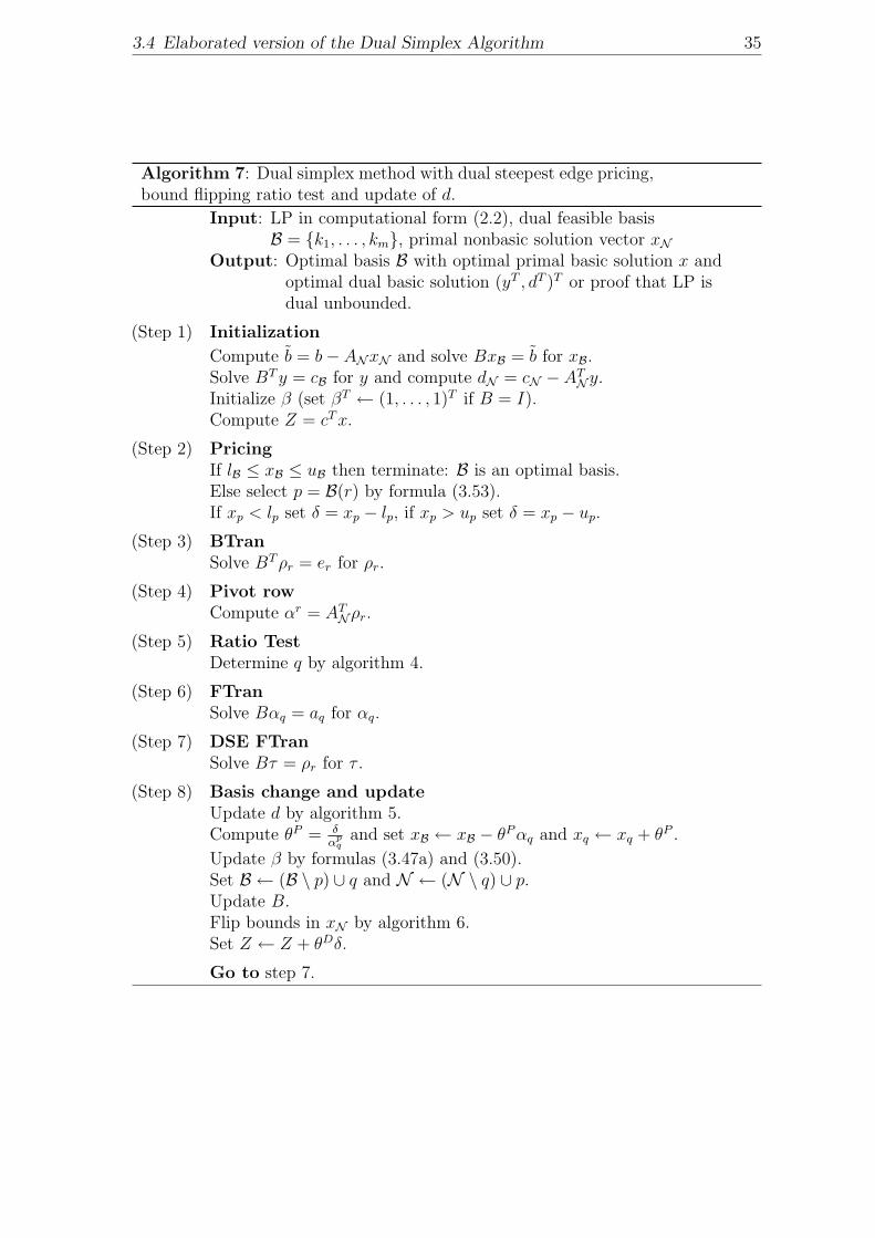
3.4 Elaborated version of the Dual Simplex Algorithm 35
Algorithm 7: Dual simplex method with dual steepest edge pricing,bound flipping ratio test and update of d.
Input: LP in computational form (2.2), dual feasible basisB = {k1, . . . , km}, primal nonbasic solution vector xN
Output: Optimal basis B with optimal primal basic solution x andoptimal dual basic solution (yT , dT )T or proof that LP isdual unbounded.
Initialization(Step 1)
Compute b = b− ANxN and solve BxB = b for xB.Solve BTy = cB for y and compute dN = cN − AT
Ny.Initialize β (set βT ← (1, . . . , 1)T if B = I).Compute Z = cTx.
Pricing(Step 2)If lB ≤ xB ≤ uB then terminate: B is an optimal basis.Else select p = B(r) by formula (3.53).If xp < lp set δ = xp − lp, if xp > up set δ = xp − up.
BTran(Step 3)Solve BTρr = er for ρr.
Pivot row(Step 4)Compute αr = AT
Nρr.
Ratio Test(Step 5)Determine q by algorithm 4.
FTran(Step 6)Solve Bαq = aq for αq.
DSE FTran(Step 7)Solve Bτ = ρr for τ .
Basis change and update(Step 8)Update d by algorithm 5.Compute θP = δ
αpq
and set xB ← xB − θPαq and xq ← xq + θP .
Update β by formulas (3.47a) and (3.50).Set B ← (B \ p) ∪ q and N ← (N \ q) ∪ p.Update B.Flip bounds in xN by algorithm 6.Set Z ← Z + θDδ.
Go to step 7.

36 Chapter 3 The Dual Simplex Method
37
Chapter 4
Dual Phase I Methods
4.1 Introduction
We refer to an algorithm which produces a dual feasible basis for an arbitrary LP asa dual phase I method. The dual simplex method presented in the previous chapteris called dual phase II in this context. Suppose in the following, that we are given a(start) basis B and a corresponding primal basic solution x and dual basic solution(yT , vT , wT )T , where v and w are set according to (2.17) with reduced costs d.
4.1.1 Big-M method
The simplest method to obtain a dual feasible basis for LP problems in computationalstandard form (2.5) (no upper bounds, nonnegative variables only) is to introducean additional dual slack variable and punish its use in the dual objective function bysome sufficiently large cost coefficient M. This is equivalent to adding a constraint ofthe form
∑j∈J xj < M to the primal problem. To apply this method to a problem
in computational form (2.2) one could convert it to a problem in standard form byintroducing additional variables and constraints. This would increase the size ofthe problem considerably. The other reason why this method is usually not used inpractise is that a high value of M can lead to numerical problems and high iterationcounts whereas a too small value might not produce a primal feasible solution. Seefor example [53] for further details. In the following, we only consider methods, thatdo not increase the size of the problem.
4.1.2 Dual feasibility correction
In most practical problems, many variables have finite lower and upper bounds. Aswe have seen in the description of the bound flipping ratio test dual infeasible boxedvariables can be made dual feasible by setting them to their respective oppositebound. As in section 3.2 we collect the variables which have to be flipped in two sets
T + = {j ∈ J : xj = lj and uj <∞ and dj < 0} (4.1a)
T − = {j ∈ J : xj = uj and lj >∞ and dj > 0}, (4.1b)
where again the variables in T + go from lower to upper bound and the variablesin T − go from upper to lower bound. Then, the primal basic variables xB and
38 Chapter 4 Dual Phase I Methods
the dual objective function value Z can be updated according to equations (3.38),(3.39) and (3.41). Algorithmicly, this is equivalent to calling algorithms 5 and 6 withθD = 0.
The above procedure is called dual feasibility correction (DFC) and can be per-formed prior to a dual phase I method. Alternatively, we can mark boxed and fixedvariables as not eligible during dual phase I, and call DFC prior to dual phase II.In any case this means, that only dual infeasibilities caused by non-boxed variableshave to be tackled by dual phase I algorithms, which is usually only a very smallfraction of the total number of variables.
4.2 Minimizing the sum of dual infeasibilities
The idea of this approach is to formulate the task of finding a dual feasible basicsolution as the subproblem of minimizing the total amount of dual infeasibility.This subproblem can be formulated as an LP problem, which can either be solveddirectly by the standard dual simplex method (phase II) or by specialized versions ofit which exploit its structural characteristics. In section 4.2.1 we present our versionof the subproblem approach which is similar to the procedure of Kostina in [41].In section 4.2.2 we will describe the algorithmic approach following Maros [48]. Itdiffers from the version described by Fourer [27] only in the way the extended ratiotest is applied: while Fourer only allows flips from dual infeasible to dual feasibleMaros also allows the contrary, both under the precondition that the sum of dualinfeasibilities decreases. To put it differently: Fourer’s algorithm is monotone bothin the sum and in the number of dual infeasibilities, while Maros’s algorithm ismonotone only in the sum of dual infeasibilities.
4.2.1 Subproblem approach
As discussed in section 4.1.2 we only have to consider dual infeasibilities associatedwith non-boxed primal variables. Let
J u = {j ∈ J : lj = −∞ and uj <∞} (4.2)
be the set of non-free variables that go dual infeasible if dj > 0,
J l = {j ∈ J : lj > −∞ and uj =∞} (4.3)
be the set of non-free variables that go dual infeasible if dj < 0 and
J f = {j ∈ J : lj = −∞ and uj =∞} (4.4)
be the set of free variables. Now, we can state the problem of finding a basis with aminimal sum of dual infeasibilities as follows:
4.2 Minimizing the sum of dual infeasibilities 39
max Z0 =∑
j∈J l∪J f
dj< 0
dj −∑
j∈J u∪J f
dj> 0
dj (4.5a)
s.t. aTj y + dj = cj for all j ∈ J l ∪ J u ∪ J f . (4.5b)
Problem (4.5) is equivalent to the following formulation:
max Z0 =∑
j∈J l∪J f
wj −∑
j∈J u∪J f
vj (4.6a)
s.t. aTj y + vj + wj = cj for all j ∈ J l ∪ J u ∪ J f (4.6b)
vj ≥ 0 (4.6c)
wj ≤ 0. (4.6d)
The dual of problem (4.6) is
min z0 =∑
j∈J l∪J u∪J f
cjxj (4.7a)
∑j∈J l∪J u∪J f
ajxj = 0 (4.7b)
− 1 ≤ xj ≤ 0 for all j ∈ J u (4.7c)
0 ≤ xj ≤ 1 for all j ∈ J l (4.7d)
− 1 ≤ xj ≤ 1 for all j ∈ J f . (4.7e)
Note, that problem (4.7) is a reduced version of our original problem (2.2) in thesense that it consists of a subset of the original set of columns and that bounds andright-hand-side is changed. Since all variables of problem (4.7) are boxed every givenstarting basis can be made dual feasible by dual feasibility correction and dual phaseII as described in algorithm 7 can directly be applied. If eventually it yields z0 = 0,we have a dual feasible basis for our original problem and can start the dual phaseII on problem (2.2). If z0 < 0, the original problem is dual infeasible. The completeapproach is summarized in algorithm 8.
Fourer mentions in [27] that for model (4.5) the dual pricing step can be simplified:only those variables need to be considered in the selection process, which will becomedual feasible after the basis change. Therefore, in our approach only those variablesare eligible to leave the basis, which go to their zero bound (being dual feasible inthe original problem).
Furthermore, we actually use a slightly modified version of the artificial prob-lem (4.7) in our implementation. To favor free variables to be pivoted into the basiswe give a weight of 104 to them in the sum of dual infeasibilities (4.5a). This trans-lates into modified individual bounds in the primal bound constraints (4.7e), whichchange to
− 104 ≤ xj ≤ 104 for all j ∈ J f . (4.8)
40 Chapter 4 Dual Phase I Methods
Algorithm 8: The 2-phases dual simplex method with subproblemdual phase I.
Input: LP in computational form (2.2).Output: Optimal basis B or proof that LP is dual unbounded.Mark boxed and fixed variables as not eligible.(Step 1)Change the bounds of the remaining variables and the(Step 2)right-hand-side vector according to problem (4.7).Start with an initial basis and make it dual feasible by dual(Step 3)feasibility correction (call algorithms 5 and 6 with θD = 0).Execute algorithm 7 on auxiliary problem (4.7).(Step 4)If z0 < 0, then original problem (2.2) is dual infeasible, stop.(Step 5)If z0 = 0, the current basis is dual feasible for problem (2.2).(Step 6)Unmark boxed and fixed variables and restore original bounds and(Step 7)right-hand-side.Execute algorithm 7 on the original problem (2.2).(Step 8)
4.2.2 Algorithmic approach
The goal of this section is to develop a specialized dual simplex type algorithm whichsolves problem (4.5). Suppose, we are given a start basis B. For easier notation wedefine two index sets
P = {j ∈ J u ∪ J f : dj > 0} (4.9)
and
M = {j ∈ J l ∪ J f : dj < 0}, (4.10)
which contain those (non-basic) variables that are dual infeasible with positive andnegative reduced costs, respectively. We do not need to consider boxed variables,since they can be made dual feasible by feasibility correction (s. section 4.1.2).
Now we can rewrite the (negative) sum of dual infeasibilities as
Z0 =∑j∈M
dj −∑j∈P
dj. (4.11)
When we relax the r-th dual basic constraint (with B(r) = p) by an amount of t thereduced costs change according to equations (3.6). If we select the leaving variableand the direction of relaxation in such a way that it will be dual feasible after thebasis change, it will not contribute to the sum of infeasibilities. Hence, as long as nononbasic dj changes sign, Z0 can be expressed as a function of t:
Z0(t) =∑j∈M
dj(t)−∑j∈P
dj(t)
4.2 Minimizing the sum of dual infeasibilities 41
=∑j∈M
(dj − tαrj)−
∑j∈P
(dj − tαrj)
= Z0 − t
(∑j∈M
αrj −
∑j∈P
αrj
)= Z0 − tfr, (4.12)
where fr is the r-the entry of the dual phase I pricing vector
f =∑j∈M
αj −∑j∈P
αj = B−1
(∑j∈M
aj −∑j∈P
aj
). (4.13)
Since we want to maximize Z0 we have to determine r and t such that −tfr ispositive. Furthermore, xp has be to dual feasible after the basis change, i.e., it hasto leave at the right finite bound given the sign of t. Hence,
if fr > 0 we need t < 0 and lB(r) > −∞ and (4.14)
if fr < 0 we need t > 0 and uB(r) <∞. (4.15)
If no such r exists, we can stop. If Z0 = 0, the current basis is dual feasible andwe can start dual phase II. If Z0 > 0, the problem is dual infeasible. Otherwise, wechoose a leaving index p = B(r) according to some reasonable pricing rule.
In the next step, we want to determine an entering index. As t is increased (ordecreased) from zero a nonbasic dual constraint j gets eligible to enter the basis whenit becomes tight, i.e., if
dj(t) = dj − tαrj = 0
⇔ t =dj
αrj
.(4.16)
Suppose for now, that t > 0. Then the set of positive breakpoints consists of thosenonbasic positions, where dj and αr
j have the same sign:
F+0 = {j ∈ N : (dj ≥ 0 and αr
j > 0) or (dj ≤ 0 and αrj < 0)}. (4.17)
If we choose the dual nonbasic constraint associated with the first (smallest) break-point to enter the basis, i.e.,
q ∈ arg minj∈F+
0
{dj
αrj
}, θD =
dq
αrq
, (4.18)
we can assure, that only this constraint possibly changes its feasibility status afterthe basis change. We refer to the selection of the entering variable according to (4.18)as simple ratio test in dual phase I.
If q is dual feasible (neither in P nor in M), then it stays dual feasible when itenters the basis and the infeasibility sets do not change. In this case, we can conclude
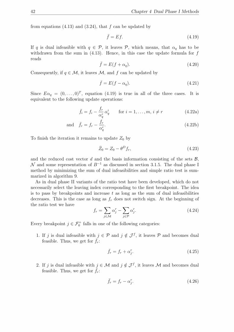
42 Chapter 4 Dual Phase I Methods
from equations (4.13) and (3.24), that f can be updated by
f = Ef. (4.19)
If q is dual infeasible with q ∈ P , it leaves P , which means, that αq has to bewithdrawn from the sum in (4.13). Hence, in this case the update formula for freads
f = E(f + αq). (4.20)
Consequently, if q ∈M, it leavesM, and f can be updated by
f = E(f − αq). (4.21)
Since Eαq = (0, . . . , 0)T , equation (4.19) is true in all of the three cases. It isequivalent to the following update operations:
fi = fi −fr
αrq
αiq for i = 1, . . . ,m, i 6= r (4.22a)
and fr = fr −fr
αrq
. (4.22b)
To finish the iteration it remains to update Z0 by
Z0 = Z0 − θDfr, (4.23)
and the reduced cost vector d and the basis information consisting of the sets B,N and some representation of B−1 as discussed in section 3.1.5. The dual phase Imethod by minimizing the sum of dual infeasibilities and simple ratio test is sum-marized in algorithm 9.
As in dual phase II variants of the ratio test have been developed, which do notnecessarily select the leaving index corresponding to the first breakpoint. The ideais to pass by breakpoints and increase t as long as the sum of dual infeasibilitiesdecreases. This is the case as long as fr does not switch sign. At the beginning ofthe ratio test we have
fr =∑j∈M
αrj −
∑j∈P
αrj . (4.24)
Every breakpoint j ∈ F+0 falls in one of the following categories:
1. If j is dual infeasible with j ∈ P and j /∈ J f , it leaves P and becomes dualfeasible. Thus, we get for fr:
fr = fr + αrj . (4.25)
2. If j is dual infeasible with j ∈ M and j /∈ J f , it leaves M and becomes dualfeasible. Thus, we get for fr:
fr = fr − αrj . (4.26)
4.2 Minimizing the sum of dual infeasibilities 43
Algorithm 9: Dual phase 1: Minimizing the sum of dual infeasibil-ities with simple ratio test.
Input: LP in computational form (2.2), start basisB = {k1, . . . , km}
Output: Dual feasible basis B with dual feasible basic solution(yT , dT )T or proof that LP is dual infeasible.
Initialization(Step 1)Solve BTy = cB for y and compute dN = cN − AT
Ny.Compute Z0 =
∑j∈M dj +
∑j∈P dj with P andM as in
equations (4.9) and (4.10).Compute a =
∑j∈M aj −
∑j∈P aj and solve Bf = a for f .
Pricing(Step 2)Let H = {i ∈ {1, . . . ,m} : (fi > 0 and lB(i) > −∞) or
(fi < 0 and lB(i) <∞)}.If H = ∅ then terminate:
If Z0 = 0, B is a dual feasible basis.If Z0 > 0, the problem is dual infeasible.
Else select r ∈ H, p = B(r) according to a reasonable pricing rule.
BTran(Step 3)Solve BTρr = er for ρr.
Pivot row(Step 4)Compute αr = AT
Nρr.
Simple ratio test(Step 5)If fr > 0 set αr = −αr, if fr < 0 set αr = αr.Let F = {j ∈ N : (dj ≥ 0 and αr
j > 0) or (dj ≤ 0 and αrj < 0)}.
Determine q ∈ arg minj∈F
{dj
αrj
}and θD = dq
αrq.
FTran(Step 6)Solve Bαq = aq for αq.
Basis change and update(Step 7)Set Z0 ← Z0 − θDf .Set dp ← −θD, dq ← 0 and dj ← dj − θDαr
j for all j ∈ N \ {q}.Set fi ← fi − fr
αrqαi
q for i = 1, . . . ,m, i 6= r and fr ← fr − fr
αrq.
Set B ← (B \ p) ∪ q and N ← (N \ q) ∪ p.Update B.
Go to step 9.
44 Chapter 4 Dual Phase I Methods
3. If j is dual infeasible with j ∈ P and j ∈ J f , it leaves P and becomes dualinfeasible with j ∈M. Thus, we get for fr:
fr = fr + 2αrj . (4.27)
4. If j is dual infeasible with j ∈ M and j ∈ J f , it leaves M and becomes dualinfeasible with j ∈ P . Thus, we get for fr:
fr = fr − 2αrj . (4.28)
5. If j is feasible and αrj < 0, it becomes dual infeasible and joins P . Thus, we
get for fr:fr = fr − αr
j . (4.29)
6. If j is feasible and αrj > 0, it becomes dual infeasible and joins M. Thus, we
get for fr:fr = fr + αr
j . (4.30)
Due to the definition of F+0 in the cases 2, 4 and 5, αr
j has to be negative. Hence,when passing a positive breakpoint, fr changes as follows:
fr = fr +
|αr
j | if j ∈ J u ∪ J l,
|αrj | if j ∈ J f and dj = 0,
2 |αrj | if j ∈ J f and dj 6= 0,.
(4.31)
Since we assume t > 0, the fr is negative in the beginning. At every breakpoint itincreases by a positive value until it eventually turns positive. This means, that theslope of Z0(t), which is −fr as shown in equation (4.12), becomes negative. At thispoint no further improvement of the sum of dual infeasibilities can be achieved andthe current breakpoint determines the entering index.
In order to be able to update the phase I pricing vector f we have to keep track ofthe changes in P and M. Let T +
P , T −P , T +M, T −M be the sets of indices, which enter
and leave P andM, respectively. Then, we get for f :
f = f +∑j∈T −P
αj −∑j∈T +
P
αj +∑
j∈T +M
αj −∑
j∈T −M
αj (4.32)
= f +B−1
∑j∈T −P
aj −∑j∈T +
P
aj +∑
j∈T +M
aj −∑
j∈T −M
aj
(4.33)
= f + ∆f, (4.34)
where ∆f is the solution of the linear system
B∆f = a, with a =∑j∈T −P
aj −∑j∈T +
P
aj +∑
j∈T +M
aj −∑
j∈T −M
aj. (4.35)
4.3 Artificial bounds 45
The extended ratio test for dual phase I is summarized in algorithm 10. For clarity,we left out the update of Z0. It can replace step 9 in algorithm 9. It is not difficultto see that the resulting algorithm is exactly the same as applying the dual phaseII (with bound flipping ratio test and the modified pricing) to the auxiliary prob-lem (4.7) (see algorithm 8). The dual phase I pricing vector f naturally correspondsto the primal basic solution vector xB in dual phase II. An advantage of the sub-problem approach is though, that no new code is needed to implement it besides thedual phase II code. Hence, every enhancement towards more numerical stability andefficiency in the dual phase II code also improves the dual phase I.
4.3 Artificial bounds
The artificial bounds method is a dual version of the composite simplex methodwhich was originally developed for the primal simplex [74]. It can be seen as a onephase approach where dual infeasible nonbasic variables are penalized in the dualobjective function by a high cost coefficient M . From the perspective of the primalproblem this means that dual infeasible variables are made dual feasible by settingthem to artificial bounds.
Suppose, some starting basis B is given and N = J \ B. We can make boxedvariables in N dual feasible by dual feasibility correction. If a variable j ∈ N is dualinfeasible at lower bound and uj =∞ , then an artificial bound uj = M is introducedand xj is set to uj (dj is not changed by this operation so j is dual feasible now). Ifa variable j ∈ N is dual infeasible at upper bound and lj = −∞, an artificial boundlj is introduced and xj is set to lj. B is dual feasible now, so we start dual phase IIwith one modification: when a variable with an artificial bound enters the basis, itsoriginal bounds are restored. If the dual phase II terminates with an optimal solutionand no nonbasic variable is at an artificial bound, we are done. If there is a nonbasicvariable j at an artificial bound, there are two possibilities: either M was chosento small to remove all of the dual infeasibilities in the final basis or the problem isprimal unbounded. To find out, we increase M (by multiplying with some constant)and start over. If M exceeds a certain threshold, we declare unboundedness.
Our first implementation of the dual simplex was based on this approach. Onedisadvantage of this method is that we do not know how large to choose M . Theright value for M heavily depends on the problem characteristic. If we choose it tosmall we risk many rounds of increasing and starting over. If we choose it to big wemight encounter numerical problems. For this reason we decided not to include thismethod in our code.
4.4 Cost modification
The basic idea of the cost modification method is similar to that of the artificialbounds method: making the starting basis dual feasible by modifying the problemformulation and restoring the original problem while executing dual phase II. Here,additionally, we may need to deploy the primal simplex method at the end.
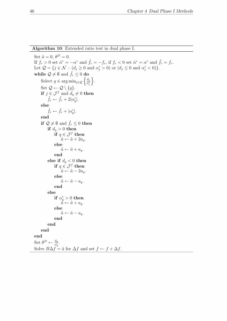
46 Chapter 4 Dual Phase I Methods
Algorithm 10: Extended ratio test in dual phase I.
Set a = 0, θD = 0.If fr > 0 set αr = −αr and fr = −fr, if fr < 0 set αr = αr and fr = fr.Let Q = {j ∈ N : (dj ≥ 0 and αr
j > 0) or (dj ≤ 0 and αrj < 0)}.
while Q 6= ∅ and fr ≤ 0 do
Select q ∈ arg minj∈Q
{dj
αrj
}.
Set Q ← Q \ {q}.if j ∈ J f and dq 6= 0 then
fr ← fr + 2|αrq|.
else
fr ← fr + |αrq|.
end
if Q 6= ∅ and fr ≤ 0 thenif dq > 0 then
if q ∈ J f thena← a+ 2aq.
elsea← a+ aq.
end
else if dq < 0 thenif q ∈ J f then
a← a− 2aq.else
a← a− aq.end
elseif αr
q > 0 thena← a+ aq.
elsea← a− aq.
end
end
end
end
Set θD ← dq
αrq.
Solve B∆f = a for ∆f and set f ← f + ∆f .
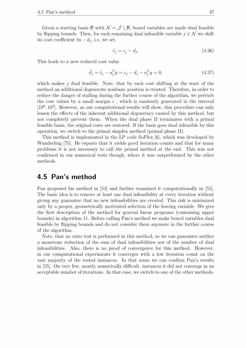
4.5 Pan’s method 47
Given a starting basis B with N = J \ B, boxed variables are made dual feasibleby flipping bounds. Then, for each remaining dual infeasible variable j ∈ N we shiftits cost coefficient by −dj, i.e, we set
cj = cj − dj. (4.36)
This leads to a new reduced cost value
dj = cj − aTj y = cj − dj − aT
j y = 0, (4.37)
which makes j dual feasible. Note, that by each cost shifting at the start of themethod an additional degenerate nonbasic position is created. Therefore, in order toreduce the danger of stalling during the further course of the algorithm, we perturbthe cost values by a small margin ε , which is randomly generated in the interval[106, 105]. However, as our computational results will show, this procedure can onlylessen the effects of the inherent additional degeneracy caused by this method, butnot completely prevent them. When the dual phase II terminates with a primalfeasible basis, the original costs are restored. If the basis goes dual infeasible by thisoperation, we switch to the primal simplex method (primal phase II).
This method is implemented in the LP code SoPlex [6], which was developed byWunderling [75]. He reports that it yields good iteration counts and that for manyproblems it is not necessary to call the primal method at the end. This was notconfirmed in our numerical tests though, where it was outperformed by the othermethods.
4.5 Pan’s method
Pan proposed his method in [54] and further examined it computationally in [55].The basic idea is to remove at least one dual infeasibility at every iteration withoutgiving any guarantee that no new infeasibilities are created. This risk is minimizedonly by a proper, geometrically motivated selection of the leaving variable. We givethe first description of the method for general linear programs (containing upperbounds) in algorithm 11. Before calling Pan’s method we make boxed variables dualfeasible by flipping bounds and do not consider them anymore in the further courseof the algorithm.
Note, that no ratio test is performed in this method, so we can guarantee neithera monotone reduction of the sum of dual infeasibilities nor of the number of dualinfeasibilities. Also, there is no proof of convergence for this method. However,in our computational experiments it converges with a low iteration count on thevast majority of the tested instances. In that sense we can confirm Pan’s resultsin [55]. On very few, mostly numerically difficult, instances it did not converge in anacceptable number of iterations. In that case, we switch to one of the other methods.
48 Chapter 4 Dual Phase I Methods
Algorithm 11: Dual phase 1: Pan’s method.
Input: LP in computational form (2.2), start basisB = {k1, . . . , km}
Output: Dual feasible basis B with dual feasible basic solution(yT , dT )T or proof that LP is dual infeasible.
Initialization(Step 1)Solve BTy = cB for y and compute dN = cN − AT
Ny.
Select entering variable(Step 2)If P ∪M = ∅ then terminate: basis is dual feasible.Else: select entering variable q ∈ arg maxj∈P∪M |dj|.
FTran(Step 3)Solve Bαq = aq for αq.
Select leaving variable(Step 4)Let H = {i ∈ {1, . . . ,m} : (lB(i) > −∞ and αi
q < 0) or(uB(i) <∞ and αi
q > 0)}.If H = ∅ then terminate: the problem is dual infeasible.Else: select leaving variable p = B(r) with r ∈ arg maxi∈H |αi
q|.
Basis change and update(Step 5)Set dp ← −θD, dq ← 0 and dj ← dj − θDαr
j for all j ∈ N \ {q}.Set B ← (B \ p) ∪ q and N ← (N \ q) ∪ p.Update B.
Go to step 9.
49
Part II
Computational techniques

51
Chapter 5
Solving Systems of Linear Equations
5.1 Introduction
The overall performance of simplex type algorithms heavily depends on the efficientsolution of systems of linear equations. In fact, four of these systems have to besolved in every iteration of the elaborated dual simplex as presented in algorithm 7(cf. section 3.4). We can distinguish two types of them. Those, which are definedby the basis matrix B, we call
FTran: Bα = a, (5.1)
and those, which are defined by its transpose BT , we call
BTran: BTπ = h. (5.2)
Efficient solution methods have to take into account the special characteristics ofthese systems and of their application within the (dual) simplex method.
• In general, the basis matrix has no special structure, is neither symmetric norpositive definite.
• Especially during the first simplex iterations the basis matrix usually containsmany unit vectors stemming from logical variables.
• The columns of the structural part of the constraint matrix normally containvery few nonzero elements. Therefore, the basis matrix stays sparse even if thebasis contains mostly structural variables.
• In every simplex iteration the basis matrix changes in only one column.
Due to these properties many classical solution methods for linear systems are notsuitable in the context of the simplex method. Conjugate gradient and other iterativemethods (see e.g. [7]) work well only for symmetric positive definite systems (or those,which can be effectively preconditioned to gain this property). Some direct methodsbased on Givens-rotations or Householder-reflextions (see e.g. [31]) have favorablenumerical features but are computationally too expensive.
In the framework of the simplex method other direct methods based on eitherthe product form of the inverse (PFI), the LU-decomposition or combinations of the
52 Chapter 5 Solving Systems of Linear Equations
two have been applied successfully. Historically, the PFI was developed shortly afterthe introduction of the simplex method (cf. [20]) and made it possible to solve LPproblems, which were considered large at that time. Later it was superseded by theLU-decomposition, which turned out to allow for a better exploitation of sparsityduring the solution process [13].
In the following we will outline the basic ideas of the PFI and LU-decomposition.In the remainder of this chapter we will focus on the latter and give detailed descrip-tions of the solution algorithms which are implemented in our code.
5.1.1 Product form of the inverse
The foundation for the PFI has been already laid out in section 3.1.5. The new basisinverse B−1 after a usual simplex basis change can be constructed by
B−1 = EB−1, (5.3)
where B−1 is the old basis inverse and E is defined according to (3.25). The ideaof the PFI is to totally avoid the explicit representation of B−1 and replace it by asequence of eta-matrices, which is used to solve the required linear systems.
For this purpose an initial set of eta-matrices has to be derived prior to the start ofthe (dual) simplex algorithm, which represents the inverse of the start basis matrixB. If B = I we are done, since I−1 = I. Otherwise, the structural columns of Bcan be successively transformed into unit vectors by Gaussian elimination1 (cf. [32,p. 94ff.]). Every elimination step yields an eta-matrix, such that finally
EsEs−1 · · ·E1B = I, (5.4)
where s with s ≤ m is the number of non-unit vectors in B. Hence, the inverse of Bcan be finally represented as
B−1 = EsEs−1 . . . E1. (5.5)
This procedure is called basis inversion. Both numerical stability and the amountof non-zero elements, which is created in the eta-matrices (called fill-in), heavilydepend on the choice of the pivot element in the elimination process. For deeperinsights into the details of the PFI inversion procedure we refer to [46, p. 122ff.], [72]and [34].
Given the sequence of k ≤ s + i − 1 eta-matrices in the i-th iteration after thebasis inversion the system (5.1) can be rewritten as
α = B−1a = EkEk−1 · · ·E1a. (5.6)
Equation (5.6) is solved recursively from right to left, the eta-matrices are appliedin the order of their generation. Therefore, this operation is called forward transfor-
1Every elimination step is equivalent to a simplex basis change starting from an identity matrixand working towards the basis matrix B by choosing a leaving column from I and an enteringcolumn from B.
5.1 Introduction 53
mation (FTran). Note, that an eta-matrix with pivot column r can be skipped, ifthe r-th entry in the current intermediate result is zero.
Likewise, system (5.2) can be written as
πT = hTB−1 = hTEkEk−1 · · ·E1 (5.7)
and solved by applying the eta-matrices from left to right, i.e., in the reversed or-der of their generation. Therefore, this operation is called backward transformation(BTran). Here, the exploitation of sparsity as in FTran is not possible. However, inevery intermediate result the number of non-zeros can at most increase by one, sinceonly the r-th entry of the result vector changes if r is the position of the eta-column.
With the number of eta-matrices numerical inaccuracies, storage requirementsand computational effort in FTran and BTran increase in every simplex iteration.Therefore, a reinversion of the basis is triggered either when a certain number ofiterations since the last inversion has passed or numerical or storage problems occur.
5.1.2 LU decomposition
Nowadays, virtually all competitive implementations of the simplex method use anLU-decomposition of the basis matrix B, which goes back to the elimination formof the inverse by Markowitz [45]. The idea is to represent the basis matrix B asa product of an upper triangular matrix U and a lower triangular matrix L2. Thegeneration process of this representation is called LU-factorization. The solution ofthe required linear systems can then be efficiently conducted by successive forwardand backward substitutions.
In the LU-factorization the basis B is transformed into an upper triangular matrixU by Gaussian elimination3. In the i-th iteration of the elimination process theelement in the upper left corner of the matrix, which has not been transformed upto this point (called active submatrix ), is chosen as pivot element. Then a lowertriangular eta-matrix Li is generated, such that
Bi+1 = Li · · ·L1B. (5.8)
After m steps Bm+1 = U is upper triangular and
Lm · · ·L1B = U. (5.9)
This form constitutes the bases for the solution of the required linear systems and theLU-update. Defining L−1 = Lm · · ·L1 and L = (L1)−1 · · · (Lm)−1 we can representB as the product of the triangular matrices L and U ,
B = LU, (5.10)
2Hence, the LU-decomposition is a representation of the basis matrix, while the PFI is a repre-sentation of the basis inverse.
3This is similar to the elimination process in the PFI-inversion, where B is transformed into theidentity matrix I.
54 Chapter 5 Solving Systems of Linear Equations
which we will refer to as the LU-factorization of B. Given (5.10) we can rewritesystem (5.1) as
LUα = a. (5.11)
By substituting Uα by α we can solve (5.11) in two independent steps. In a firststep we solve
FTranL: Lα = a ⇔ α = L−1a (5.12)
by applying the eta-matrices produced during LU-factorization to a, then we solve
FTranU: Uα = α (5.13)
by backward substitution. The same can be done for system (5.2) with
UTLTπ = h (5.14)
by substituting LTπ by π and solving
BTranU: UT π = h (5.15)
for π followed by computing
BTranL: LTπ = π ⇔ α = (LT )−1a (5.16)
for π.
5.2 LU factorization
Numerical stability and the amount of fill-in during the Gaussian elimination pro-cedure depend heavily on the choice of the pivot elements during the factorizationprocedure. To be free to choose a pivot element, which is advantageous with respectto these two goals, row and column permutations are applied to B in every iteration.The result can be represented in the form
LU = PBQ, (5.17)
where L and U are lower and upper triangular matrices, respectively, P is a row-and Q is a column permutation matrix. By defining permuted versions L = P−1LPand U = P−1UQ−1 of L and U equation (5.17) transforms to
PLP−1PUQ = PBQ (5.18)
⇔ LU = B (5.19)
⇔ L−1B = U (5.20)
⇔ L−1B = P−1UQ−1. (5.21)
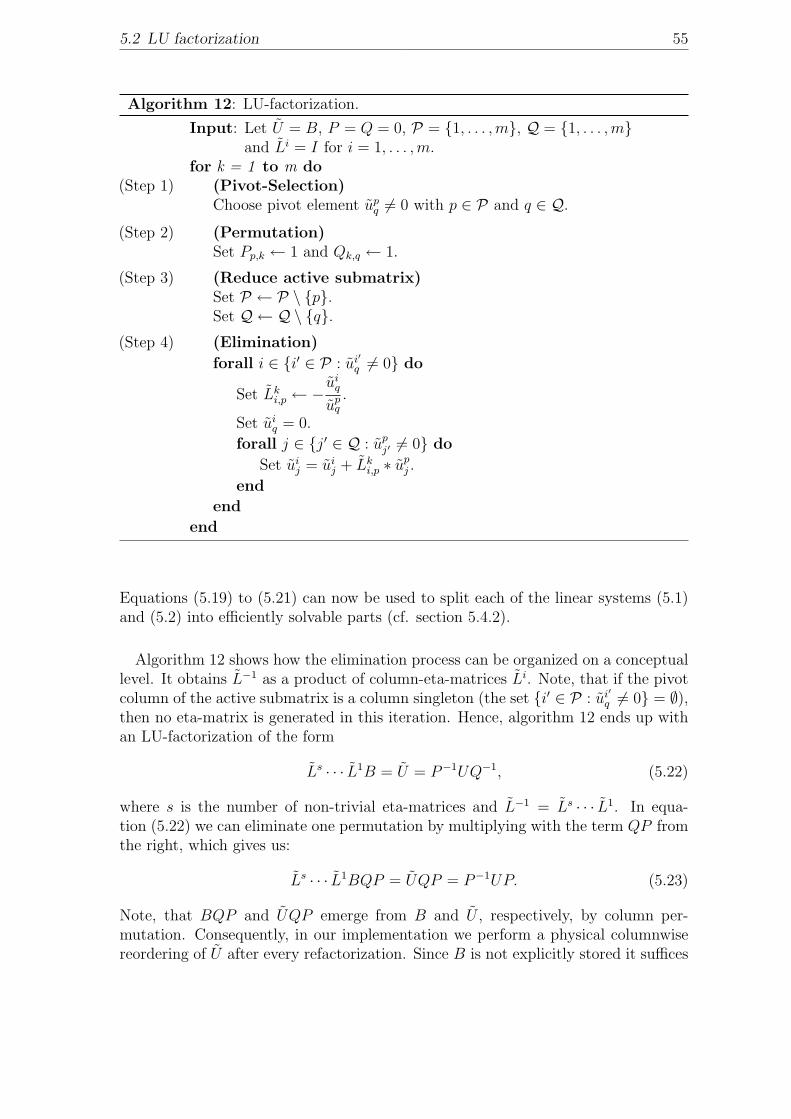
5.2 LU factorization 55
Algorithm 12: LU-factorization.
Input: Let U = B, P = Q = 0, P = {1, . . . ,m}, Q = {1, . . . ,m}and Li = I for i = 1, . . . ,m.
for k = 1 to m do(Pivot-Selection)(Step 1)Choose pivot element up
q 6= 0 with p ∈ P and q ∈ Q.
(Permutation)(Step 2)Set Pp,k ← 1 and Qk,q ← 1.
(Reduce active submatrix)(Step 3)Set P ← P \ {p}.Set Q ← Q \ {q}.(Elimination)(Step 4)
forall i ∈ {i′ ∈ P : ui′q 6= 0} do
Set Lki,p ← −
uiq
upq.
Set uiq = 0.
forall j ∈ {j′ ∈ Q : upj′ 6= 0} do
Set uij = ui
j + Lki,p ∗ u
pj .
end
end
end
Equations (5.19) to (5.21) can now be used to split each of the linear systems (5.1)and (5.2) into efficiently solvable parts (cf. section 5.4.2).
Algorithm 12 shows how the elimination process can be organized on a conceptuallevel. It obtains L−1 as a product of column-eta-matrices Li. Note, that if the pivotcolumn of the active submatrix is a column singleton (the set {i′ ∈ P : ui′
q 6= 0} = ∅),then no eta-matrix is generated in this iteration. Hence, algorithm 12 ends up withan LU-factorization of the form
Ls · · · L1B = U = P−1UQ−1, (5.22)
where s is the number of non-trivial eta-matrices and L−1 = Ls · · · L1. In equa-tion (5.22) we can eliminate one permutation by multiplying with the term QP fromthe right, which gives us:
Ls · · · L1BQP = UQP = P−1UP. (5.23)
Note, that BQP and UQP emerge from B and U , respectively, by column per-mutation. Consequently, in our implementation we perform a physical columnwisereordering of U after every refactorization. Since B is not explicitly stored it suffices
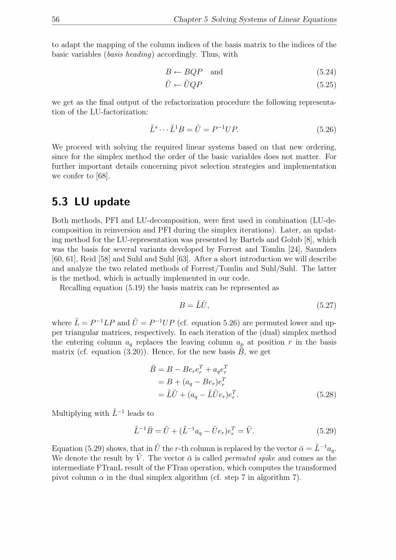
56 Chapter 5 Solving Systems of Linear Equations
to adapt the mapping of the column indices of the basis matrix to the indices of thebasic variables (basis heading) accordingly. Thus, with
B ← BQP and (5.24)
U ← UQP (5.25)
we get as the final output of the refactorization procedure the following representa-tion of the LU-factorization:
Ls · · · L1B = U = P−1UP. (5.26)
We proceed with solving the required linear systems based on that new ordering,since for the simplex method the order of the basic variables does not matter. Forfurther important details concerning pivot selection strategies and implementationwe confer to [68].
5.3 LU update
Both methods, PFI and LU-decomposition, were first used in combination (LU-de-composition in reinversion and PFI during the simplex iterations). Later, an updat-ing method for the LU-representation was presented by Bartels and Golub [8], whichwas the basis for several variants developed by Forrest and Tomlin [24], Saunders[60, 61], Reid [58] and Suhl and Suhl [63]. After a short introduction we will describeand analyze the two related methods of Forrest/Tomlin and Suhl/Suhl. The latteris the method, which is actually implemented in our code.
Recalling equation (5.19) the basis matrix can be represented as
B = LU , (5.27)
where L = P−1LP and U = P−1UP (cf. equation 5.26) are permuted lower and up-per triangular matrices, respectively. In each iteration of the (dual) simplex methodthe entering column aq replaces the leaving column ap at position r in the basismatrix (cf. equation (3.20)). Hence, for the new basis B, we get
B = B −BereTr + aqe
Tr
= B + (aq −Ber)eTr
= LU + (aq − LUer)eTr . (5.28)
Multiplying with L−1 leads to
L−1B = U + (L−1aq − Uer)eTr = V . (5.29)
Equation (5.29) shows, that in U the r-th column is replaced by the vector α = L−1aq.We denote the result by V . The vector α is called permuted spike and comes as theintermediate FTranL result of the FTran operation, which computes the transformedpivot column α in the dual simplex algorithm (cf. step 7 in algorithm 7).
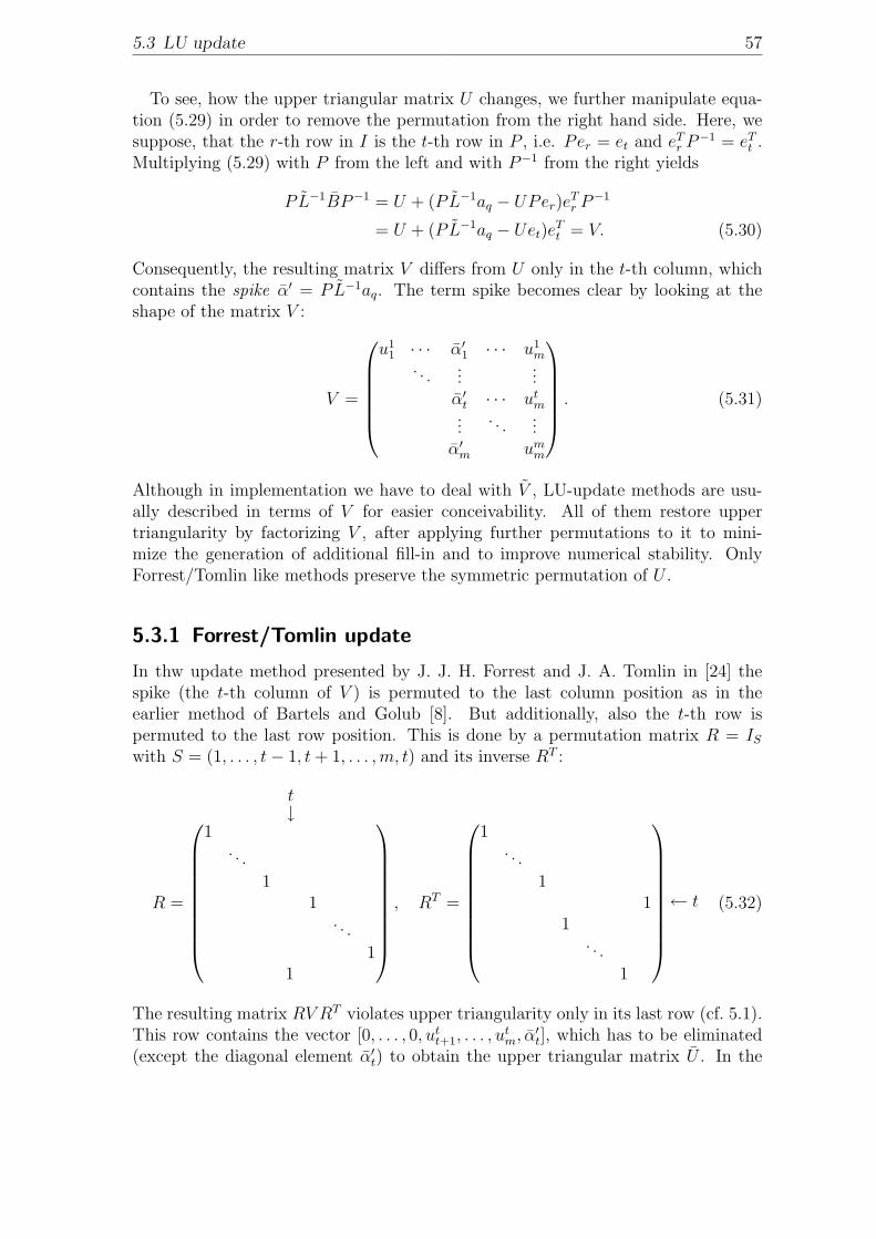
5.3 LU update 57
To see, how the upper triangular matrix U changes, we further manipulate equa-tion (5.29) in order to remove the permutation from the right hand side. Here, wesuppose, that the r-th row in I is the t-th row in P , i.e. Per = et and eT
r P−1 = eT
t .Multiplying (5.29) with P from the left and with P−1 from the right yields
PL−1BP−1 = U + (PL−1aq − UPer)eTr P
−1
= U + (PL−1aq − Uet)eTt = V. (5.30)
Consequently, the resulting matrix V differs from U only in the t-th column, whichcontains the spike α′ = PL−1aq. The term spike becomes clear by looking at theshape of the matrix V :
V =
u1
1 · · · α′1 · · · u1m
. . ....
...α′t · · · ut
m...
. . ....
α′m umm
. (5.31)
Although in implementation we have to deal with V , LU-update methods are usu-ally described in terms of V for easier conceivability. All of them restore uppertriangularity by factorizing V , after applying further permutations to it to mini-mize the generation of additional fill-in and to improve numerical stability. OnlyForrest/Tomlin like methods preserve the symmetric permutation of U .
5.3.1 Forrest/Tomlin update
In thw update method presented by J. J. H. Forrest and J. A. Tomlin in [24] thespike (the t-th column of V ) is permuted to the last column position as in theearlier method of Bartels and Golub [8]. But additionally, also the t-th row ispermuted to the last row position. This is done by a permutation matrix R = ISwith S = (1, . . . , t− 1, t+ 1, . . . ,m, t) and its inverse RT :
t↓
R =
1. . .
11
. . .
11
, RT =
1. . .
11
1. . .
1
← t (5.32)
The resulting matrix RV RT violates upper triangularity only in its last row (cf. 5.1).This row contains the vector [0, . . . , 0, ut
t+1, . . . , utm, α
′t], which has to be eliminated
(except the diagonal element α′t) to obtain the upper triangular matrix U . In the
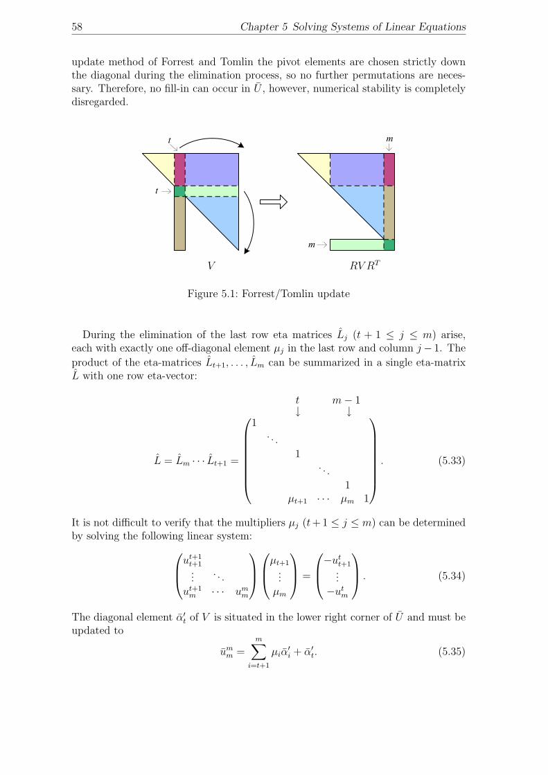
58 Chapter 5 Solving Systems of Linear Equations
update method of Forrest and Tomlin the pivot elements are chosen strictly downthe diagonal during the elimination process, so no further permutations are neces-sary. Therefore, no fill-in can occur in U , however, numerical stability is completelydisregarded.
r
t
t
r
t
r
W W
t
l
t
0 0. . . 0 0. . .
t
r
t
r
r tr
m
m
m
l
l
t
V RV RT
Figure 5.1: Forrest/Tomlin update
During the elimination of the last row eta matrices Lj (t + 1 ≤ j ≤ m) arise,each with exactly one off-diagonal element µj in the last row and column j− 1. The
product of the eta-matrices Lt+1, . . . , Lm can be summarized in a single eta-matrixL with one row eta-vector:
t m− 1↓ ↓
L = Lm · · · Lt+1 =
1. . .
1. . .
1µt+1 · · · µm 1
. (5.33)
It is not difficult to verify that the multipliers µj (t+1 ≤ j ≤ m) can be determinedby solving the following linear system:u
t+1t+1...
. . .
ut+1m · · · um
m
µt+1
...µm
=
−utt+1...−ut
m
. (5.34)
The diagonal element α′t of V is situated in the lower right corner of U and must beupdated to
umm =
m∑i=t+1
µiα′i + α′t. (5.35)
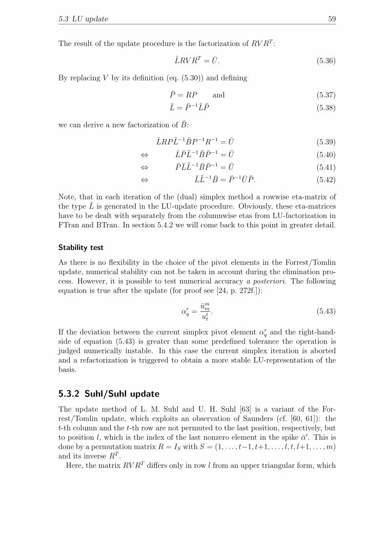
5.3 LU update 59
The result of the update procedure is the factorization of RV RT :
LRV RT = U . (5.36)
By replacing V by its definition (eq. (5.30)) and defining
P = RP and (5.37)
L = P−1LP (5.38)
we can derive a new factorization of B:
LRPL−1BP−1R−1 = U (5.39)
⇔ LP L−1BP−1 = U (5.40)
⇔ P LL−1BP−1 = U (5.41)
⇔ LL−1B = P−1U P . (5.42)
Note, that in each iteration of the (dual) simplex method a rowwise eta-matrix ofthe type L is generated in the LU-update procedure. Obviously, these eta-matriceshave to be dealt with separately from the columnwise etas from LU-factorization inFTran and BTran. In section 5.4.2 we will come back to this point in greater detail.
Stability test
As there is no flexibility in the choice of the pivot elements in the Forrest/Tomlinupdate, numerical stability can not be taken in account during the elimination pro-cess. However, it is possible to test numerical accuracy a posteriori. The followingequation is true after the update (for proof see [24, p. 272f.]):
αrq =
umm
utt
. (5.43)
If the deviation between the current simplex pivot element αrq and the right-hand-
side of equation (5.43) is greater than some predefined tolerance the operation isjudged numerically instable. In this case the current simplex iteration is abortedand a refactorization is triggered to obtain a more stable LU-representation of thebasis.
5.3.2 Suhl/Suhl update
The update method of L. M. Suhl and U. H. Suhl [63] is a variant of the For-rest/Tomlin update, which exploits an observation of Saunders (cf. [60, 61]): thet-th column and the t-th row are not permuted to the last position, respectively, butto position l, which is the index of the last nonzero element in the spike α′. This isdone by a permutation matrix R = IS with S = (1, . . . , t−1, t+1, . . . , l, t, l+1, . . . ,m)and its inverse RT .
Here, the matrix RV RT differs only in row l from an upper triangular form, which
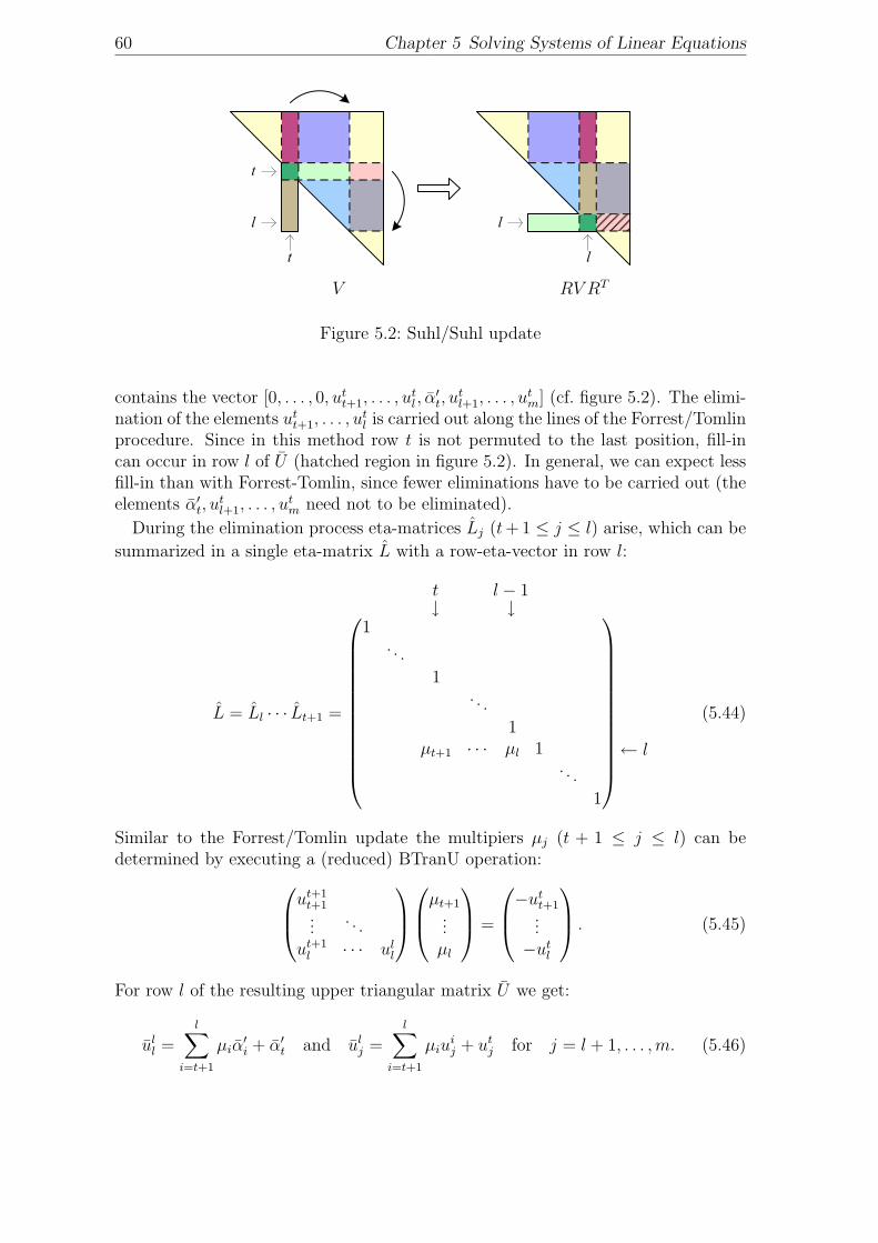
60 Chapter 5 Solving Systems of Linear Equations
r
t
t
r
t
r
W W
t
l
t
0 0. . . 0 0. . .
t
r
t
r
r tr
m
m
m
l
l
t
V RV RT
Figure 5.2: Suhl/Suhl update
contains the vector [0, . . . , 0, utt+1, . . . , u
tl , α
′t, u
tl+1, . . . , u
tm] (cf. figure 5.2). The elimi-
nation of the elements utt+1, . . . , u
tl is carried out along the lines of the Forrest/Tomlin
procedure. Since in this method row t is not permuted to the last position, fill-incan occur in row l of U (hatched region in figure 5.2). In general, we can expect lessfill-in than with Forrest-Tomlin, since fewer eliminations have to be carried out (theelements α′t, u
tl+1, . . . , u
tm need not to be eliminated).
During the elimination process eta-matrices Lj (t+ 1 ≤ j ≤ l) arise, which can be
summarized in a single eta-matrix L with a row-eta-vector in row l:
t l − 1↓ ↓
L = Ll · · · Lt+1 =
1. . .
1. . .
1µt+1 · · · µl 1
. . .
1
← l
(5.44)
Similar to the Forrest/Tomlin update the multipiers µj (t + 1 ≤ j ≤ l) can bedetermined by executing a (reduced) BTranU operation:u
t+1t+1...
. . .
ut+1l · · · ul
l
µt+1
...µl
=
−utt+1...−ut
l
. (5.45)
For row l of the resulting upper triangular matrix U we get:
ull =
l∑i=t+1
µiα′i + α′t and ul
j =l∑
i=t+1
µiuij + ut
j for j = l + 1, . . . ,m. (5.46)
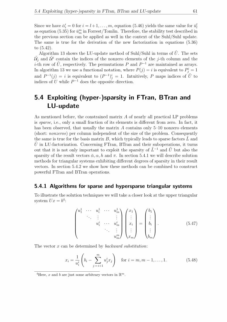
5.4 Exploiting (hyper-)sparsity in FTran, BTran and LU-update 61
Since we have α′i = 0 for i = l+1, . . . ,m, equation (5.46) yields the same value for ull
as equation (5.35) for umm in Forrest/Tomlin. Therefore, the stability test described in
the previous section can be applied as well in the context of the Suhl/Suhl update.The same is true for the derivation of the new factorization in equations (5.36)to (5.42).
Algorithm 13 shows the LU-update method of Suhl/Suhl in terms of U . The setsUj and U i contain the indices of the nonzero elements of the j-th column and thei-th row of U , respectively. The permutations P and P−1 are maintained as arrays.In algorithm 13 we use a functional notation, where P (j) = i is equivalent to P i
j = 1
and P−1(j) = i is equivalent to (P−1)ij = 1. Intuitively, P maps indices of U to
indices of U while P−1 does the opposite direction.
5.4 Exploiting (hyper-)sparsity in FTran, BTran andLU-update
As mentioned before, the constrained matrix A of nearly all practical LP problemsis sparse, i.e., only a small fraction of its elements is different from zero. In fact, ithas been observed, that usually the matrix A contains only 5–10 nonzero elements(short: nonzeros) per column independent of the size of the problem. Consequentlythe same is true for the basis matrix B, which typically leads to sparse factors L andU in LU-factorization. Concerning FTran, BTran and their suboperations, it turnsout that it is not only important to exploit the sparsity of L−1 and U but also thesparsity of the result vectors α, α, h and π. In section 5.4.1 we will describe solutionmethods for triangular systems exhibiting different degrees of sparsity in their resultvectors. In section 5.4.2 we show how these methods can be combined to constructpowerful FTran and BTran operations.
5.4.1 Algorithms for sparse and hypersparse triangular systems
To illustrate the solution techniques we will take a closer look at the upper triangularsystem Ux = b4:
u11 · · · u1
i · · · u1m
. . ....
...ui
i · · · uim
. . ....um
m
x1...xi...xm
=
b1...bi...bm
. (5.47)
The vector x can be determined by backward substitution:
xi =1
uii
(bi −
m∑j = i+1
uijxj
)for i = m,m− 1, . . . , 1. (5.48)
4Here, x and b are just some arbitrary vectors in Rm.
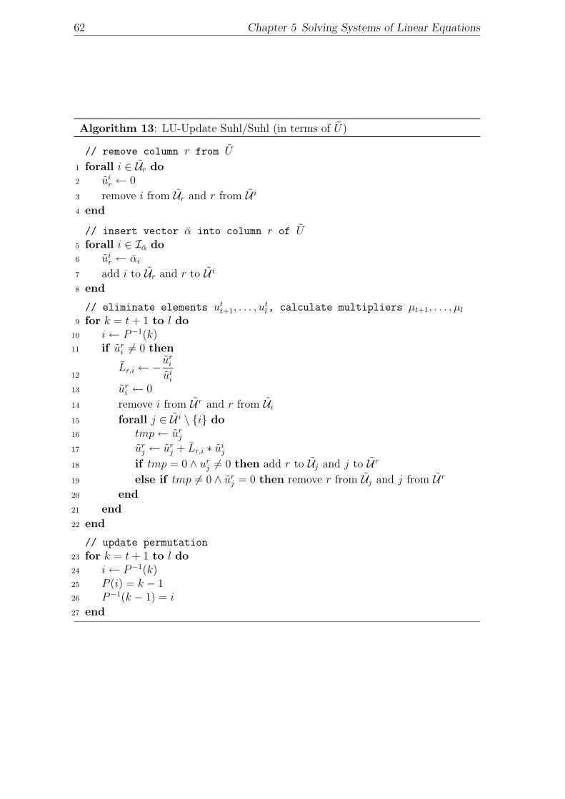
62 Chapter 5 Solving Systems of Linear Equations
Algorithm 13: LU-Update Suhl/Suhl (in terms of U)
// remove column r from U
forall i ∈ Ur do1
uir ← 02
remove i from Ur and r from U i3
end4
// insert vector α into column r of Uforall i ∈ Iα do5
uir ← αi6
add i to Ur and r to U i7
end8
// eliminate elements utt+1, . . . , u
tl, calculate multipliers µt+1, . . . , µl
for k = t+ 1 to l do9
i← P−1(k)10
if uri 6= 0 then11
Lr,i ← −ur
i
uii
12
uri ← 013
remove i from U r and r from Ui14
forall j ∈ U i \ {i} do15
tmp← urj16
urj ← ur
j + Lr,i ∗ uij17
if tmp = 0 ∧ urj 6= 0 then add r to Uj and j to U r
18
else if tmp 6= 0 ∧ urj = 0 then remove r from Uj and j from U r
19
end20
end21
end22
// update permutation
for k = t+ 1 to l do23
i← P−1(k)24
P (i) = k − 125
P−1(k − 1) = i26
end27
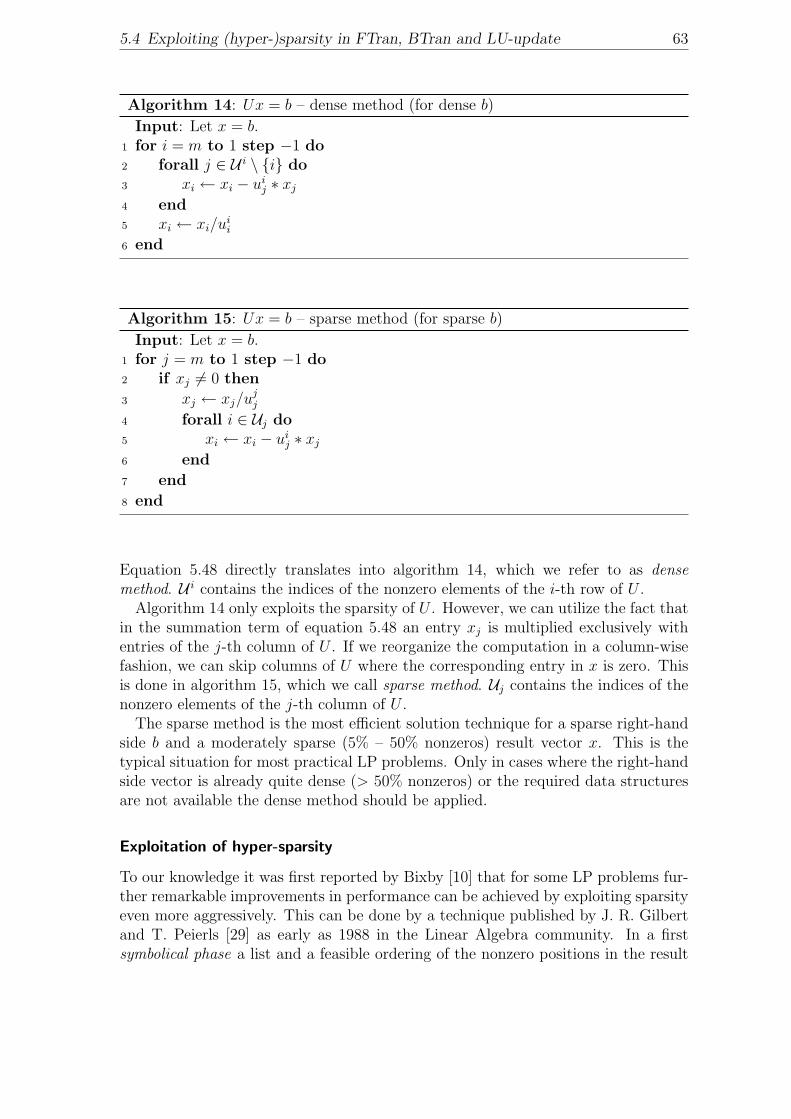
5.4 Exploiting (hyper-)sparsity in FTran, BTran and LU-update 63
Algorithm 14: Ux = b – dense method (for dense b)
Input: Let x = b.for i = m to 1 step −1 do1
forall j ∈ U i \ {i} do2
xi ← xi − uij ∗ xj3
end4
xi ← xi/uii5
end6
Algorithm 15: Ux = b – sparse method (for sparse b)
Input: Let x = b.for j = m to 1 step −1 do1
if xj 6= 0 then2
xj ← xj/ujj3
forall i ∈ Uj do4
xi ← xi − uij ∗ xj5
end6
end7
end8
Equation 5.48 directly translates into algorithm 14, which we refer to as densemethod. U i contains the indices of the nonzero elements of the i-th row of U .
Algorithm 14 only exploits the sparsity of U . However, we can utilize the fact thatin the summation term of equation 5.48 an entry xj is multiplied exclusively withentries of the j-th column of U . If we reorganize the computation in a column-wisefashion, we can skip columns of U where the corresponding entry in x is zero. Thisis done in algorithm 15, which we call sparse method. Uj contains the indices of thenonzero elements of the j-th column of U .
The sparse method is the most efficient solution technique for a sparse right-handside b and a moderately sparse (5% – 50% nonzeros) result vector x. This is thetypical situation for most practical LP problems. Only in cases where the right-handside vector is already quite dense (> 50% nonzeros) or the required data structuresare not available the dense method should be applied.
Exploitation of hyper-sparsity
To our knowledge it was first reported by Bixby [10] that for some LP problems fur-ther remarkable improvements in performance can be achieved by exploiting sparsityeven more aggressively. This can be done by a technique published by J. R. Gilbertand T. Peierls [29] as early as 1988 in the Linear Algebra community. In a firstsymbolical phase a list and a feasible ordering of the nonzero positions in the result
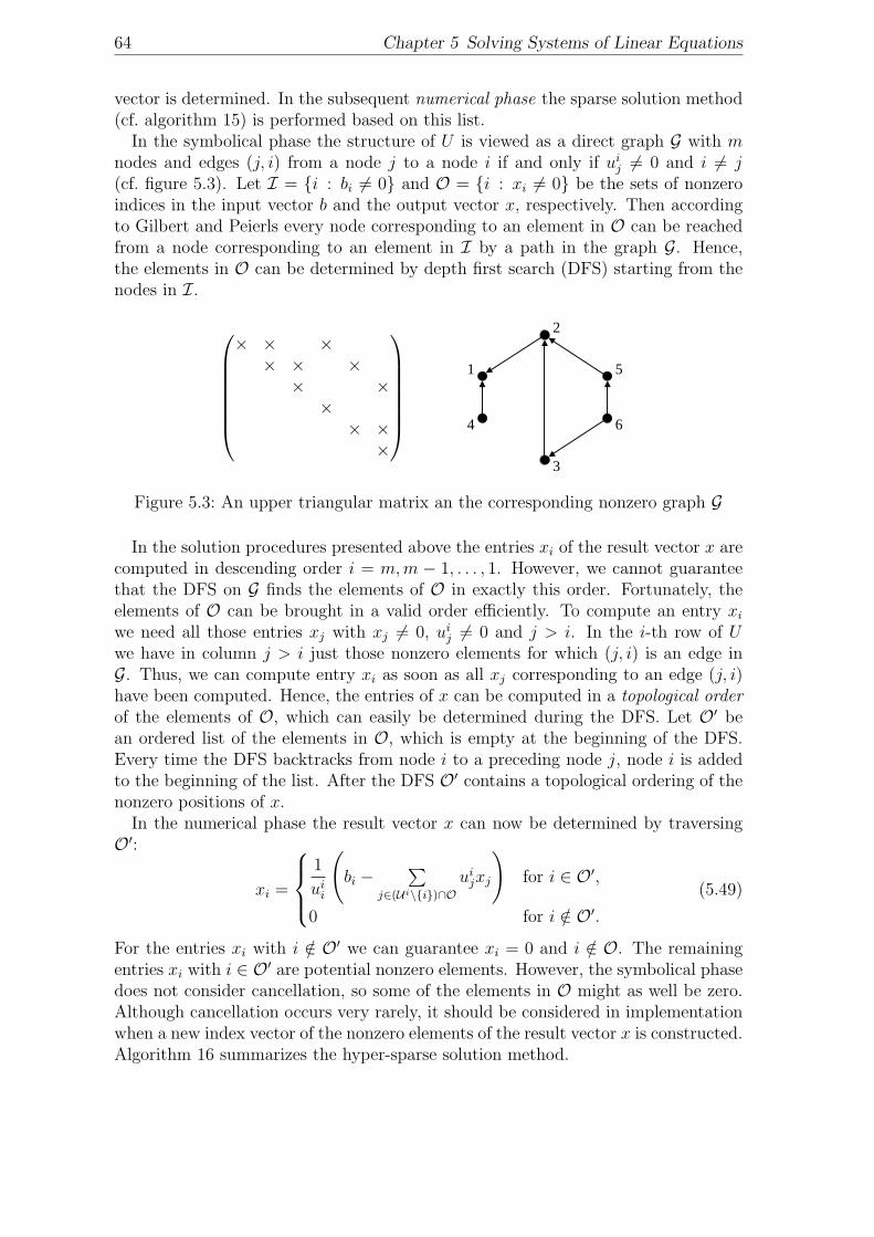
64 Chapter 5 Solving Systems of Linear Equations
vector is determined. In the subsequent numerical phase the sparse solution method(cf. algorithm 15) is performed based on this list.
In the symbolical phase the structure of U is viewed as a direct graph G with mnodes and edges (j, i) from a node j to a node i if and only if ui
j 6= 0 and i 6= j(cf. figure 5.3). Let I = {i : bi 6= 0} and O = {i : xi 6= 0} be the sets of nonzeroindices in the input vector b and the output vector x, respectively. Then accordingto Gilbert and Peierls every node corresponding to an element in O can be reachedfrom a node corresponding to an element in I by a path in the graph G. Hence,the elements in O can be determined by depth first search (DFS) starting from thenodes in I.
× × ×× × ×× ××× ××
4444 84444 764444 84444 76
rlenrbeg
mi1
row i
i ...
valcindcptr
...
...
... ...
...
...
...
col i
i ...
rptrrindcval
...
...
...
... ...
...
...
#
cbegclen
mi1
...
...
...
...
...
...
...
...# #
# # #
freespace
freespace
L-1
L-1
val...
lbeg
...
1...
netaf 2
......
...
......
neta
freespace
etas from LUF
rind.........*...*
cind*............
U
*
⎪⎪⎪⎪
⎭
⎪⎪⎪⎪
⎬
⎫
⎪⎪⎪⎪
⎭
⎪⎪⎪⎪
⎬
⎫
row-wise U
col-wise U
etas from LUU
1 netaf...etacol
1 mcoleta
j
lenlulbeg(neta+1)+1 lbeg(netaf+1) lbeg(netaf+1)+1
1
4
3
6
5
2
lastrowlastcol
p
...
......
r
s
lbeg(1)
lstart
Figure 5.3: An upper triangular matrix an the corresponding nonzero graph G
In the solution procedures presented above the entries xi of the result vector x arecomputed in descending order i = m,m − 1, . . . , 1. However, we cannot guaranteethat the DFS on G finds the elements of O in exactly this order. Fortunately, theelements of O can be brought in a valid order efficiently. To compute an entry xi
we need all those entries xj with xj 6= 0, uij 6= 0 and j > i. In the i-th row of U
we have in column j > i just those nonzero elements for which (j, i) is an edge inG. Thus, we can compute entry xi as soon as all xj corresponding to an edge (j, i)have been computed. Hence, the entries of x can be computed in a topological orderof the elements of O, which can easily be determined during the DFS. Let O′ bean ordered list of the elements in O, which is empty at the beginning of the DFS.Every time the DFS backtracks from node i to a preceding node j, node i is addedto the beginning of the list. After the DFS O′ contains a topological ordering of thenonzero positions of x.
In the numerical phase the result vector x can now be determined by traversingO′:
xi =
1
uii
(bi −
∑j∈(Ui\{i})∩O
uijxj
)for i ∈ O′,
0 for i /∈ O′.(5.49)
For the entries xi with i /∈ O′ we can guarantee xi = 0 and i /∈ O. The remainingentries xi with i ∈ O′ are potential nonzero elements. However, the symbolical phasedoes not consider cancellation, so some of the elements in O might as well be zero.Although cancellation occurs very rarely, it should be considered in implementationwhen a new index vector of the nonzero elements of the result vector x is constructed.Algorithm 16 summarizes the hyper-sparse solution method.
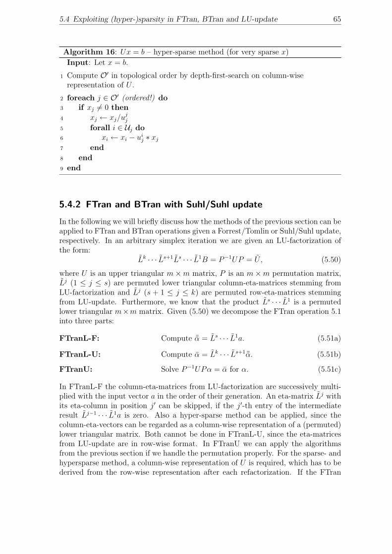
5.4 Exploiting (hyper-)sparsity in FTran, BTran and LU-update 65
Algorithm 16: Ux = b – hyper-sparse method (for very sparse x)
Input: Let x = b.
Compute O′ in topological order by depth-first-search on column-wise1
representation of U .
foreach j ∈ O′ (ordered!) do2
if xj 6= 0 then3
xj ← xj/ujj4
forall i ∈ Uj do5
xi ← xi − uij ∗ xj6
end7
end8
end9
5.4.2 FTran and BTran with Suhl/Suhl update
In the following we will briefly discuss how the methods of the previous section can beapplied to FTran and BTran operations given a Forrest/Tomlin or Suhl/Suhl update,respectively. In an arbitrary simplex iteration we are given an LU-factorization ofthe form:
Lk · · · Ls+1Ls · · · L1B = P−1UP = U , (5.50)
where U is an upper triangular m×m matrix, P is an m×m permutation matrix,Lj (1 ≤ j ≤ s) are permuted lower triangular column-eta-matrices stemming fromLU-factorization and Lj (s + 1 ≤ j ≤ k) are permuted row-eta-matrices stemmingfrom LU-update. Furthermore, we know that the product Ls · · · L1 is a permutedlower triangular m×m matrix. Given (5.50) we decompose the FTran operation 5.1into three parts:
FTranL-F: Compute ¯α = Ls · · · L1a. (5.51a)
FTranL-U: Compute α = Lk · · · Ls+1 ¯α. (5.51b)
FTranU: Solve P−1UPα = α for α. (5.51c)
In FTranL-F the column-eta-matrices from LU-factorization are successively multi-plied with the input vector a in the order of their generation. An eta-matrix Lj withits eta-column in position j′ can be skipped, if the j′-th entry of the intermediateresult Lj−1 · · · L1a is zero. Also a hyper-sparse method can be applied, since thecolumn-eta-vectors can be regarded as a column-wise representation of a (permuted)lower triangular matrix. Both cannot be done in FTranL-U, since the eta-matricesfrom LU-update are in row-wise format. In FTranU we can apply the algorithmsfrom the previous section if we handle the permutation properly. For the sparse- andhypersparse method, a column-wise representation of U is required, which has to bederived from the row-wise representation after each refactorization. If the FTran
66 Chapter 5 Solving Systems of Linear Equations
operation is called to compute the transformed incoming column, α is saved afterFTranL-U to be used as spike in LU-update.
Similarly, the BTran operation 5.2 is decomposed into three parts
BTranU: Solve P−1UTPπ = h for π. (5.52a)
BTranL-U: Compute ¯π = (Ls+1)T · · · (Lk)T π. (5.52b)
BTranL-F: Compute π = (L1)T · · · (Ls)T ¯π. (5.52c)
As in FTranU the slightly modified version of the sparse- and hypersparse solutionalgorithms 15 and 16 can as well be applied in BTranU. Here, forward substitu-tion has to be performed on a row-wise representation of U (which is equivalentto a columnwise representation of UT ). As before the permutation can be handledefficiently. In BTranL-U the same techniques can be applied (which was not pos-sible in FTranL-U), since the row-eta-vectors represent the non-trivial columns ofthe transposed eta-matrices (Ls+1)T , . . . , (Lk)T . However, in BTranL-F a row-wiserepresentation of the product Ls · · · L1 would be required to exploit sparsity andhypersparsity of π. This is not done in our implementation.
67
Chapter 6
Numerical Stability and Degeneracy
6.1 Introduction
It might seem as a minimum requirement for an implemented numerical algorithmthat it terminates after a finite period of time with a correct answer for any prob-lem instance belonging to the class of problems it was designed for. Unfortunately,even if the algorithm can be proved to be correct with respect to these two goalson a theoretical basis, the same cannot be guaranteed for its implementation in acomputational environment, which can only handle floating point numbers of finiteprecision. For the simplex algorithm the situation is even worse: for the commonlyused pivot selection rules we can not even theoretically guarantee termination due tothe possibility of getting into an infinite cycle of degenerate bases. While this typeof pure cycling occurs rarely for practical LP problems degeneracy often retards con-vergence by preventing improvement of the objective function for many consecutiveiterations (called stalling). Together with numerical inaccuracies the thread of nu-merical cycling arises, where small deteriorations in the objective function may leadinto an infinite loop.
For these reasons we have to be more modest and lower our requirements to thefollowing goal: our code should give sufficiently correct results for the widest possiblerange of LP problems or otherwise, fail in a controlled manner. In this chapter wewill discuss methods, which have been proposed in the literature and used in otherpublicly available codes, and present the variants which we incorporated into theMOPS dual simplex code to improve numerical stability, handle inaccuracies andreduce the number of degenerate iterations. But before we come to methods we willcharacterize the notions of numerical stability and degeneracy in more detail.
6.1.1 Numerical stability
As we mentioned before the representation of floating point numbers as well as allarithmetic operations are of limited precision on commonly used computer technol-ogy. On modern PC-environments 64-bit1 arithmetic leads to a relative numericalerror in the order of 10−16. Analyzing the numerical stability of an algorithms meansto understand how and under which circumstances these inevitable inaccuracies cangrow and accumulate and in the worst case, lead to unusable results. In the follow-
1Internally modern processor even work with 80-bit arithmetic. The results are then converted to64-bit.
68 Chapter 6 Numerical Stability and Degeneracy
ing we will discuss two results from the field of numerical error analysis, which areimportant in the context of the (dual) simplex algorithm.
The first one is an elementary result from backward error analysis of linear systems.Our presentation is similar to [31, p. 50ff.]. Let B be a nonsingular m ×m-matrixand consider the linear system
Bx = b (6.1)
with right-hand-side b and exact solution x. Let ∆B and ∆b be perturbations of theproblem data B and b such that x+∆xb and x+∆xB are solutions of the perturbedsystems
B(x+ ∆xb) = b+ ∆b (6.2)
and(B + ∆B)(x+ ∆xB) = b, (6.3)
respectively. With these notations it is easy to see that the following upper boundshold for the relative error of the solution vector2:
‖∆xb‖‖x‖
≤ ‖B−1‖‖B‖‖∆b‖‖b‖
(6.4)
and‖∆xB‖‖x+ ∆xB‖
≤ ‖B−1‖‖B‖‖∆B‖‖B‖
. (6.5)
In both of the inequalities the term ‖B−1‖‖B‖ reflects the maximum possible changein the exact solution of a linear system induced by a change in the data. This quantityis called condition number of a nonsingular matrix B and is defined by
cond(b) = ‖B−1‖‖B‖. (6.6)
From (6.4) and (6.5) we can conclude that for a well conditioned matrix B, wherecond(B) ≈ 1, the relative error in the solution vector x can not be much greater thanthe inaccuracies in the problem data (possibly resulting from limited floating pointprecision). On the other hand for an ill conditioned matrix B, where cond(B)� 1,small errors in the problem data can lead to great changes in the solution of thelinear system.
We want to emphasize that the condition number is totally problem dependentand can be determined a priori to its solution (which is very expensive though). Inthe context of the simplex method often the condition of an optimal basis is takenas a measure for the numerical difficulty of an LP problem. While the simplexmethod must terminate with an optimal basis, the path it takes to reach this basisgreatly depends upon the deployed pivot selection strategies. Often, even problems,which are well conditioned around their optimal solution, feature regions of badlyconditioned bases in their space of basic solutions. The goal of numerically stableimplementations must be to avoid these regions or leave them as soon as possiblewhen numerical difficulties occurred.
2Here we denote by ‖ · ‖ the euclidian norm with respect to vectors and the corresponding subor-dinate norm w.r.t. matrices such that ‖B‖ = sup‖x‖=1 ‖Bx‖.
6.1 Introduction 69
The second long known result from error analysis (proof e.g. in [75, p. 54f.]) showshow the condition might evolve in a simplex basis change. If B denotes the new basismatrix, which emanates from the old basis matrix B according to equation (5.28),then the following upper bound on the condition number of the new basis can bederived:
cond(B) ≤ 1
|αrq|· (1 + ‖αq‖) · (1 + ‖αq‖+ |αr
q|) · cond(B) (6.7)
The main consequence of inequality (6.7) is that small pivot elements should beavoided to prevent a substantial increase of the condition number in a basis change.In section 6.2.2 we will therefore discuss techniques to avoid the selection of smallpivot element in the simple and in the bound flipping dual ratio test. Unfortunately,these techniques cannot guarantee stability under all possible circumstances, so weneed further strategies to detect and to handle numerical problems during the solu-tion process. In particular we must minimize if not eliminate the risk of numericalcycling. Such strategies are summarized in section 6.2.3. The remainder of thechapter is devoted to techniques to lessen the detrimental effects of degeneracy.
6.1.2 Degeneracy and cycling
When we talk about degeneracy in this section we always mean dual degeneracy asit is defined in section 2.4. In a degenerate iteration of the dual simplex methodthe entering variable has zero reduced costs, which results in a dual step length ofzero and prevents an improvement of the objective function value. Note, that in thebound flipping ratio test, a degenerate basis does not necessarily lead to a degenerateiteration. Within a sequence of degenerate iterations and separated by the samesuccession of entering and leaving variables the same basis can occur repeatedly andthe method can get stuck in an infinite cycle. This phenomenon is called cycling.In non-degenerate iterations the method proceeds exclusively to bases with strictlyincreasing objective function values, so no basis can be repeated. On some problems,sequences of degenerate iterations can get very long even if no cycling occurs andslow down the solution process considerably. Cunningham [17] introduced the termstalling to describe this behavior.
As we have learned in the previous section finite precision arithmetic almost alwaysleads to tiny numerical inaccuracies in the results of practically all arithmetic oper-ations. In the simplex method these inaccuracies act as small perturbations whichresolve ties in the ratio test. This is often said to be the reason why pure cyclingas defined above is very unlikely to occur in practise. Wunderling [75, p. 60] pointsout though, that nowadays simplex algorithms are often deployed to solve the LPrelaxations of large, highly degenerated combinatorial optimization problems. Theseproblems typically feature perfectly conditioned 0/1 constraint matrices such thatvirtually no numerical perturbations occur and degeneracy persists in its pure form.On these problems, the effects of stalling aggravate and pure cycling poses a realthread, which has to be handled properly.
Especially on badly conditioned problems and also as a possible consequence ofHarris’ ratio test (cf. section 6.2.2.1), small backward steps in the objective function
70 Chapter 6 Numerical Stability and Degeneracy
can occur, sometimes even accompanied by a loss of dual feasibility. When theobjective function value and the basic solution oscillate by very small amounts insubsequent iterations numerical cycling can occur, although there is no degeneracypresent in the strict sense. This situation is well described in [25]. It constitutes oneof the major challenges to stability in implementations of the simplex method.
Bland [12] was the first, who developed a pivot selection strategy (smallest sub-script or Bland’s rule) which guaranties termination of the simplex method in thepresence of degeneracy. Unfortunately, it turned out to be inefficient in practise sinceit leads to a very large number of iterations. Since then, several anti-cycling andanti-degeneracy techniques with better practical behavior have been proposed. Themost established are Wolfe’s ’ad hoc’ method [74, 59], perturbation techniques likethe one described in [9], the EXPAND procedure of [30] and shifting strategies likein [75, p. 60f.]. A good overview and description of these techniques can be foundin [46, p. 230ff.]. They also seem to be well suited to prevent numerical cycling.While these techniques mainly effect the dual ratio test it is well known that dualsteepest edge pricing (as described in section 3.3) can greatly reduce the numberof degenerate iterations (especially in conjunction with perturbation). In our testsalso a simple way of resolving ties in pricing by randomization turned out to be veryuseful to reduce stalling and diminish the risk of cycling.
In section 6.3 we will present the strategies which we incorporated into our code.They are based on the above ideas and came to our knowledge through the COINLP implementation of the dual simplex method [44].
6.2 Techniques to ensure numerical stability
The overall strategy of our code to prevent numerical failure consists of three pillars:
1. A numerically stable LU-factorization and -update procedure. Computation ofthe initial primal and dual basic solutions (after refactorization) with highestpossible precision.
2. A stabilizing ratio test, which avoids the selection of small pivot elements.Prohibition of very small pivot elements.
3. A ”multi-layer safety net” consisting of techniques like e.g. numerical accuracychecks, optional abortion and restart of an iteration and double checking beforereporting final results.
Regarding the LU-factorization we confer to section 5.2 and [68]. The main focusof this section lies on the points 2 (section 6.2.2) and 3 (section 6.2.3). We start byintroducing the concept of numerical tolerances.
6.2.1 Numerical tolerances
The most important underlying computational technique to realize these strategiesis the use of numerical tolerances. Table 6.1 gives an overview including notationand default values in our implementation. By the first two feasibility tolerances the
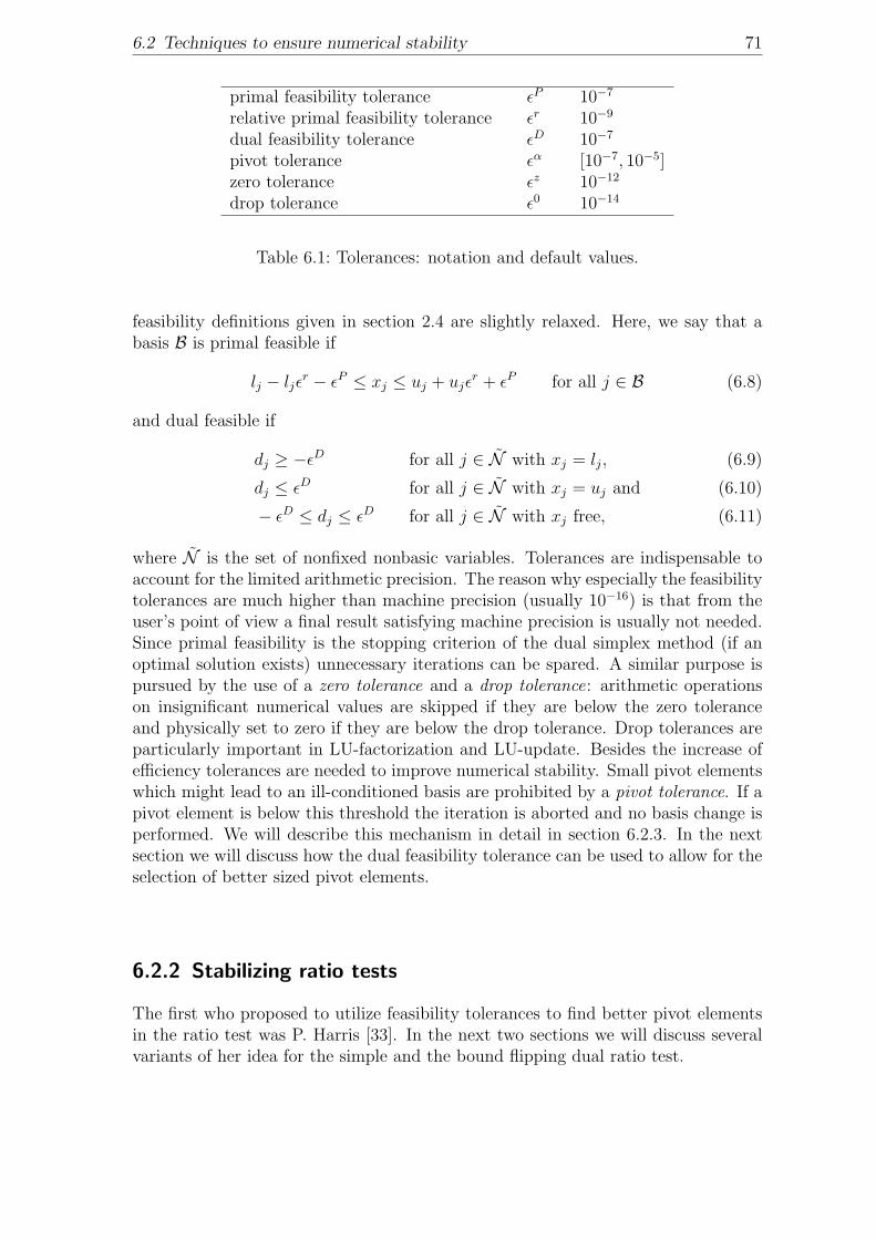
6.2 Techniques to ensure numerical stability 71
primal feasibility tolerance εP 10−7
relative primal feasibility tolerance εr 10−9
dual feasibility tolerance εD 10−7
pivot tolerance εα [10−7, 10−5]zero tolerance εz 10−12
drop tolerance ε0 10−14
Table 6.1: Tolerances: notation and default values.
feasibility definitions given in section 2.4 are slightly relaxed. Here, we say that abasis B is primal feasible if
lj − ljεr − εP ≤ xj ≤ uj + ujεr + εP for all j ∈ B (6.8)
and dual feasible if
dj ≥ −εD for all j ∈ N with xj = lj, (6.9)
dj ≤ εD for all j ∈ N with xj = uj and (6.10)
− εD ≤ dj ≤ εD for all j ∈ N with xj free, (6.11)
where N is the set of nonfixed nonbasic variables. Tolerances are indispensable toaccount for the limited arithmetic precision. The reason why especially the feasibilitytolerances are much higher than machine precision (usually 10−16) is that from theuser’s point of view a final result satisfying machine precision is usually not needed.Since primal feasibility is the stopping criterion of the dual simplex method (if anoptimal solution exists) unnecessary iterations can be spared. A similar purpose ispursued by the use of a zero tolerance and a drop tolerance: arithmetic operationson insignificant numerical values are skipped if they are below the zero toleranceand physically set to zero if they are below the drop tolerance. Drop tolerances areparticularly important in LU-factorization and LU-update. Besides the increase ofefficiency tolerances are needed to improve numerical stability. Small pivot elementswhich might lead to an ill-conditioned basis are prohibited by a pivot tolerance. If apivot element is below this threshold the iteration is aborted and no basis change isperformed. We will describe this mechanism in detail in section 6.2.3. In the nextsection we will discuss how the dual feasibility tolerance can be used to allow for theselection of better sized pivot elements.
6.2.2 Stabilizing ratio tests
The first who proposed to utilize feasibility tolerances to find better pivot elementsin the ratio test was P. Harris [33]. In the next two sections we will discuss severalvariants of her idea for the simple and the bound flipping dual ratio test.
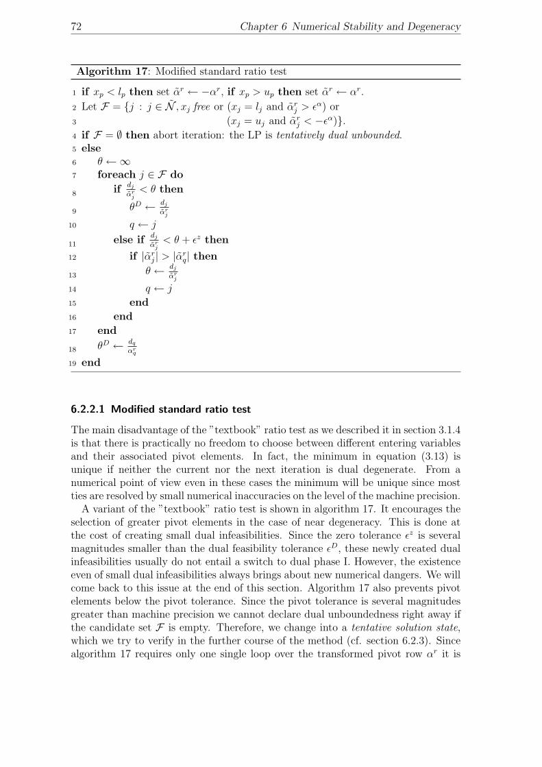
72 Chapter 6 Numerical Stability and Degeneracy
Algorithm 17: Modified standard ratio test
if xp < lp then set αr ← −αr, if xp > up then set αr ← αr.1
Let F = {j : j ∈ N , xj free or (xj = lj and αrj > εα) or2
(xj = uj and αrj < −εα)}.3
if F = ∅ then abort iteration: the LP is tentatively dual unbounded.4
else5
θ ←∞6
foreach j ∈ F do7
ifdj
αrj< θ then8
θD ← dj
αrj
9
q ← j10
else ifdj
αrj< θ + εz then11
if |αrj | > |αr
q| then12
θ ← dj
αrj
13
q ← j14
end15
end16
end17
θD ← dq
αrq
18
end19
6.2.2.1 Modified standard ratio test
The main disadvantage of the ”textbook” ratio test as we described it in section 3.1.4is that there is practically no freedom to choose between different entering variablesand their associated pivot elements. In fact, the minimum in equation (3.13) isunique if neither the current nor the next iteration is dual degenerate. From anumerical point of view even in these cases the minimum will be unique since mostties are resolved by small numerical inaccuracies on the level of the machine precision.
A variant of the ”textbook” ratio test is shown in algorithm 17. It encourages theselection of greater pivot elements in the case of near degeneracy. This is done atthe cost of creating small dual infeasibilities. Since the zero tolerance εz is severalmagnitudes smaller than the dual feasibility tolerance εD, these newly created dualinfeasibilities usually do not entail a switch to dual phase I. However, the existenceeven of small dual infeasibilities always brings about new numerical dangers. We willcome back to this issue at the end of this section. Algorithm 17 also prevents pivotelements below the pivot tolerance. Since the pivot tolerance is several magnitudesgreater than machine precision we cannot declare dual unboundedness right away ifthe candidate set F is empty. Therefore, we change into a tentative solution state,which we try to verify in the further course of the method (cf. section 6.2.3). Sincealgorithm 17 requires only one single loop over the transformed pivot row αr it is
6.2 Techniques to ensure numerical stability 73
called a one-pass ratio test.
6.2.2.2 Harris’ ratio test
To increase the flexibility of the ratio test even further, Harris [33] proposed to acceptthe creation of infeasibilities within the full range of the feasibility tolerance. We willdescribe her approach in the context of the dual ratio test for the case t ≥ 0. In a firststep (or pass) a bound Θmax on the dual step length θD is computed which ensuresthat the respective strict dual feasibility conditions of the nonbasic nonfixed variablesare not violated by more than the dual feasibility tolerance. For this purpose we splitthe candidate set F+ as define in equation (3.12) into two subsets
F+l = {j ∈ N : (xj free or xj = lj) and αr
j > 0} and (6.12)
F+u = {j ∈ N : (xj free or xj = uj) and αr
j < 0}. (6.13)
Then it is not difficult to see that Θmax can be computed as follows:
Θmax = min
{minj∈F+
l
{dj + εD
αrj
}, minj∈F+
u
{dj − εD
αrj
}}. (6.14)
In a second pass, among all breakpoints which do not exceed the bound Θmax theone with the pivot element of greatest absolute value |αr
j | is chosen to determine theentering variable and the dual step length:
q ∈ arg maxj∈F+
{|αr
j | :dj
αrj
≤ Θmax
}and θD =
dq
αrq
. (6.15)
Undoubtedly, Harris’ ratio test yields better sized pivot elements and therefore limitsthe deterioration of the basis condition in the LU-update. However, it also comeswith two severe disadvantages:
1. The method requires in principle two passes of the transformed pivot row αr.Although the second pass can be limited to the elements in the candidate setF+, the computational effort is considerably higher compared to a one passmethod.
2. The creation of small dual infeasibilities is an inherent property of this ratiotest. If the methods selects such a slightly dual infeasible variable as leav-ing variable, the corresponding breakpoint and therefore the dual step lengthwill be of wrong sign. This can have two perilous consequences. Firstly, thedual objective function will move into the wrong direction which brings upthe danger of numerical cycling. Secondly, during the update of the reducedcost vector other nonbasic variables belonging to the candidate set F− can bepushed beyond the dual feasibility tolerance. This will provoke a call to thedual phase I, which again results in a decreasing objective function value andthe thread of numerical cycling. To understand why this case can actually hap-pen, imagine a nonbasic variable j ∈ F− with xj = lj, which is already at the
74 Chapter 6 Numerical Stability and Degeneracy
edge of dual infeasibility with dj = −εD. Even the smallest move with a dualstep length θD < 0 would push this variable beyond the tolerance. Although
in the case of backward steps the dual step length is bounded by −∣∣∣ εD
αrq
∣∣∣ from
below, variables in F− move by an amount of∣∣∣εD αr
j
αrq
∣∣∣ towards their infeasibil-
ity bound (or pass it by this amount in the worst case), which can be a highmultiple of the feasibility tolerance.
In implementation we skip candidates with pivot elements that fall below the pivottolerance (as in algorithm 17). We also made some good experiences with a variant,where we use a special tolerance εH instead of εD in equation 6.14. Depending on thecurrent numerical status εH varies between εz and εD (a typical value is 0.01 ∗ εD).The idea is to find a good compromise between the need for better pivot elementsin numerically difficult situations and the unnecessary creation of significant dualinfeasibilities. Note, that with εH < εD it may happen that Θmax < 0 if a reducedcost value dj is slightly dual infeasible with εH < |dj| ≤ εD. This case can actuallyoccur since we always have to anticipate dual infeasibilites up to the dual feasibilitytolerance, which is also the stopping criterion for dual phase I. Theoretically it is noproblem but it has to be considered properly in implementation.
6.2.2.3 Shifting
As mentioned before we always have to be able to deal with dual infeasibilities withinthe tolerance in the dual ratio test, no matter wether we use a Harris variant or not.This is true due to two main reasons: 1. Usually, the dual phase I is terminatedwhen no dual infeasibility exceeds a certain phase I feasibility tolerance εD1 (e.g.εD1 = 0.1 ∗ εD). So there may still exist dual infeasibilities below this tolerance. 2.For numerically very difficult problems, numerical errors can reach the level of thefeasibility tolerances. One consequence can be that new dual infeasibilities (above orbelow the tolerance) occur after the recomputation of the reduced cost in the contextof a refactorization.
While the above variant of Harris ratio test reduces the danger of ”really” loosingdual feasibility (resulting in a call to dual phase I), we still have to avoid backwardsteps to rule out the risk of numerical cycling. The main approach to do this is calledshifting and was worked out in detail for the primal simplex method in [30] in thecontext of the anti-cycling procedure EXPAND. The idea is to locally manipulate theproblem data to avoid the negative step. For the dual simplex method this meansmanipulations of cost coefficients. We discussed the same idea in section 4.4 as away to make an arbitrary basis dual feasible. Here, we use it to achieve a zero oreven slightly positive dual step length and still fulfill the dual basic constraint forthe entering variable, such that dq = 0 after the basis change.
Suppose, that we have determined a dual step length θD = dq
αrq< 0 at the end of
the dual ratio test. Then the following is done:
1. Set θD ← 0 (or alternatively: θD ← 10−12).
2. Compute shift ∆q ← θDαrq − dq.
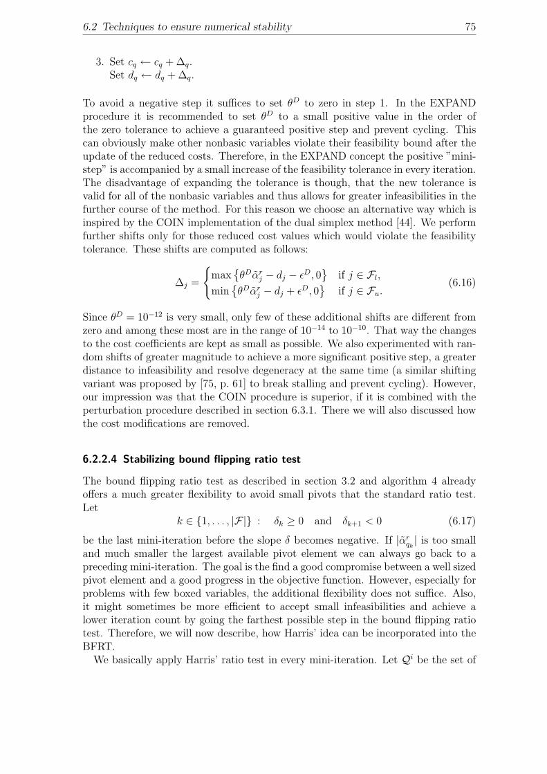
6.2 Techniques to ensure numerical stability 75
3. Set cq ← cq + ∆q.Set dq ← dq + ∆q.
To avoid a negative step it suffices to set θD to zero in step 1. In the EXPANDprocedure it is recommended to set θD to a small positive value in the order ofthe zero tolerance to achieve a guaranteed positive step and prevent cycling. Thiscan obviously make other nonbasic variables violate their feasibility bound after theupdate of the reduced costs. Therefore, in the EXPAND concept the positive ”mini-step” is accompanied by a small increase of the feasibility tolerance in every iteration.The disadvantage of expanding the tolerance is though, that the new tolerance isvalid for all of the nonbasic variables and thus allows for greater infeasibilities in thefurther course of the method. For this reason we choose an alternative way which isinspired by the COIN implementation of the dual simplex method [44]. We performfurther shifts only for those reduced cost values which would violate the feasibilitytolerance. These shifts are computed as follows:
∆j =
{max
{θDαr
j − dj − εD, 0}
if j ∈ Fl,
min{θDαr
j − dj + εD, 0}
if j ∈ Fu.(6.16)
Since θD = 10−12 is very small, only few of these additional shifts are different fromzero and among these most are in the range of 10−14 to 10−10. That way the changesto the cost coefficients are kept as small as possible. We also experimented with ran-dom shifts of greater magnitude to achieve a more significant positive step, a greaterdistance to infeasibility and resolve degeneracy at the same time (a similar shiftingvariant was proposed by [75, p. 61] to break stalling and prevent cycling). However,our impression was that the COIN procedure is superior, if it is combined with theperturbation procedure described in section 6.3.1. There we will also discussed howthe cost modifications are removed.
6.2.2.4 Stabilizing bound flipping ratio test
The bound flipping ratio test as described in section 3.2 and algorithm 4 alreadyoffers a much greater flexibility to avoid small pivots that the standard ratio test.Let
k ∈ {1, . . . , |F|} : δk ≥ 0 and δk+1 < 0 (6.17)
be the last mini-iteration before the slope δ becomes negative. If |αrqk| is too small
and much smaller the largest available pivot element we can always go back to apreceding mini-iteration. The goal is the find a good compromise between a well sizedpivot element and a good progress in the objective function. However, especially forproblems with few boxed variables, the additional flexibility does not suffice. Also,it might sometimes be more efficient to accept small infeasibilities and achieve alower iteration count by going the farthest possible step in the bound flipping ratiotest. Therefore, we will now describe, how Harris’ idea can be incorporated into theBFRT.
We basically apply Harris’ ratio test in every mini-iteration. Let Qi be the set of
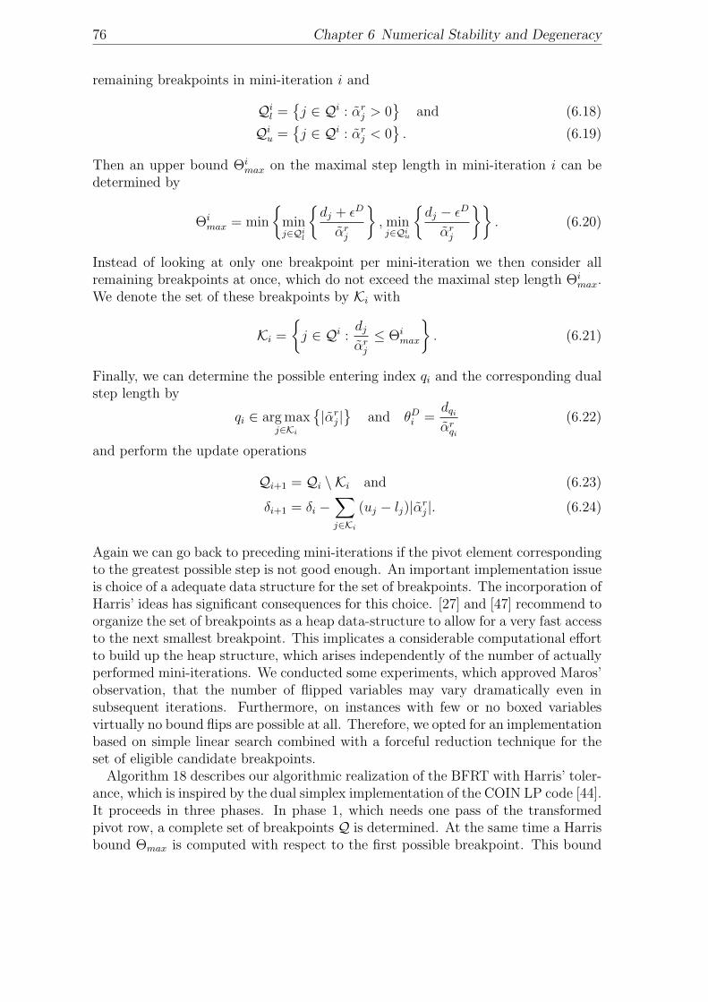
76 Chapter 6 Numerical Stability and Degeneracy
remaining breakpoints in mini-iteration i and
Qil =
{j ∈ Qi : αr
j > 0}
and (6.18)
Qiu =
{j ∈ Qi : αr
j < 0}. (6.19)
Then an upper bound Θimax on the maximal step length in mini-iteration i can be
determined by
Θimax = min
{minj∈Qi
l
{dj + εD
αrj
}, minj∈Qi
u
{dj − εD
αrj
}}. (6.20)
Instead of looking at only one breakpoint per mini-iteration we then consider allremaining breakpoints at once, which do not exceed the maximal step length Θi
max.We denote the set of these breakpoints by Ki with
Ki =
{j ∈ Qi :
dj
αrj
≤ Θimax
}. (6.21)
Finally, we can determine the possible entering index qi and the corresponding dualstep length by
qi ∈ arg maxj∈Ki
{|αr
j |}
and θDi =
dqi
αrqi
(6.22)
and perform the update operations
Qi+1 = Qi \ Ki and (6.23)
δi+1 = δi −∑j∈Ki
(uj − lj)|αrj |. (6.24)
Again we can go back to preceding mini-iterations if the pivot element correspondingto the greatest possible step is not good enough. An important implementation issueis choice of a adequate data structure for the set of breakpoints. The incorporation ofHarris’ ideas has significant consequences for this choice. [27] and [47] recommend toorganize the set of breakpoints as a heap data-structure to allow for a very fast accessto the next smallest breakpoint. This implicates a considerable computational effortto build up the heap structure, which arises independently of the number of actuallyperformed mini-iterations. We conducted some experiments, which approved Maros’observation, that the number of flipped variables may vary dramatically even insubsequent iterations. Furthermore, on instances with few or no boxed variablesvirtually no bound flips are possible at all. Therefore, we opted for an implementationbased on simple linear search combined with a forceful reduction technique for theset of eligible candidate breakpoints.
Algorithm 18 describes our algorithmic realization of the BFRT with Harris’ toler-ance, which is inspired by the dual simplex implementation of the COIN LP code [44].It proceeds in three phases. In phase 1, which needs one pass of the transformedpivot row, a complete set of breakpoints Q is determined. At the same time a Harrisbound Θmax is computed with respect to the first possible breakpoint. This bound
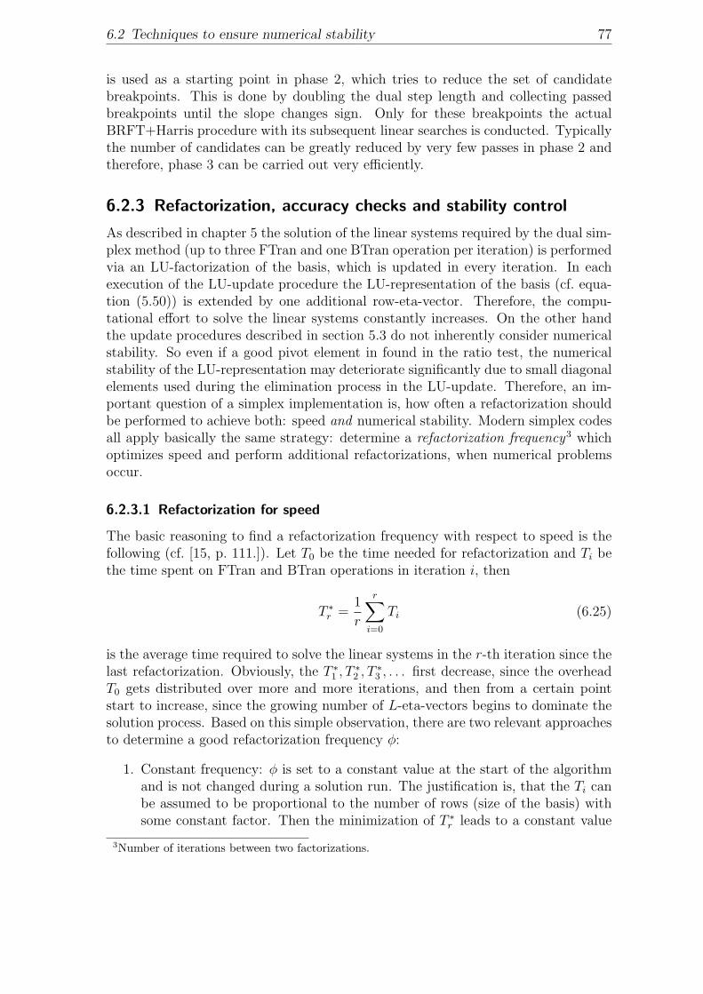
6.2 Techniques to ensure numerical stability 77
is used as a starting point in phase 2, which tries to reduce the set of candidatebreakpoints. This is done by doubling the dual step length and collecting passedbreakpoints until the slope changes sign. Only for these breakpoints the actualBRFT+Harris procedure with its subsequent linear searches is conducted. Typicallythe number of candidates can be greatly reduced by very few passes in phase 2 andtherefore, phase 3 can be carried out very efficiently.
6.2.3 Refactorization, accuracy checks and stability control
As described in chapter 5 the solution of the linear systems required by the dual sim-plex method (up to three FTran and one BTran operation per iteration) is performedvia an LU-factorization of the basis, which is updated in every iteration. In eachexecution of the LU-update procedure the LU-representation of the basis (cf. equa-tion (5.50)) is extended by one additional row-eta-vector. Therefore, the compu-tational effort to solve the linear systems constantly increases. On the other handthe update procedures described in section 5.3 do not inherently consider numericalstability. So even if a good pivot element in found in the ratio test, the numericalstability of the LU-representation may deteriorate significantly due to small diagonalelements used during the elimination process in the LU-update. Therefore, an im-portant question of a simplex implementation is, how often a refactorization shouldbe performed to achieve both: speed and numerical stability. Modern simplex codesall apply basically the same strategy: determine a refactorization frequency3 whichoptimizes speed and perform additional refactorizations, when numerical problemsoccur.
6.2.3.1 Refactorization for speed
The basic reasoning to find a refactorization frequency with respect to speed is thefollowing (cf. [15, p. 111.]). Let T0 be the time needed for refactorization and Ti bethe time spent on FTran and BTran operations in iteration i, then
T ∗r =1
r
r∑i=0
Ti (6.25)
is the average time required to solve the linear systems in the r-th iteration since thelast refactorization. Obviously, the T ∗1 , T
∗2 , T
∗3 , . . . first decrease, since the overhead
T0 gets distributed over more and more iterations, and then from a certain pointstart to increase, since the growing number of L-eta-vectors begins to dominate thesolution process. Based on this simple observation, there are two relevant approachesto determine a good refactorization frequency φ:
1. Constant frequency: φ is set to a constant value at the start of the algorithmand is not changed during a solution run. The justification is, that the Ti canbe assumed to be proportional to the number of rows (size of the basis) withsome constant factor. Then the minimization of T ∗r leads to a constant value
3Number of iterations between two factorizations.
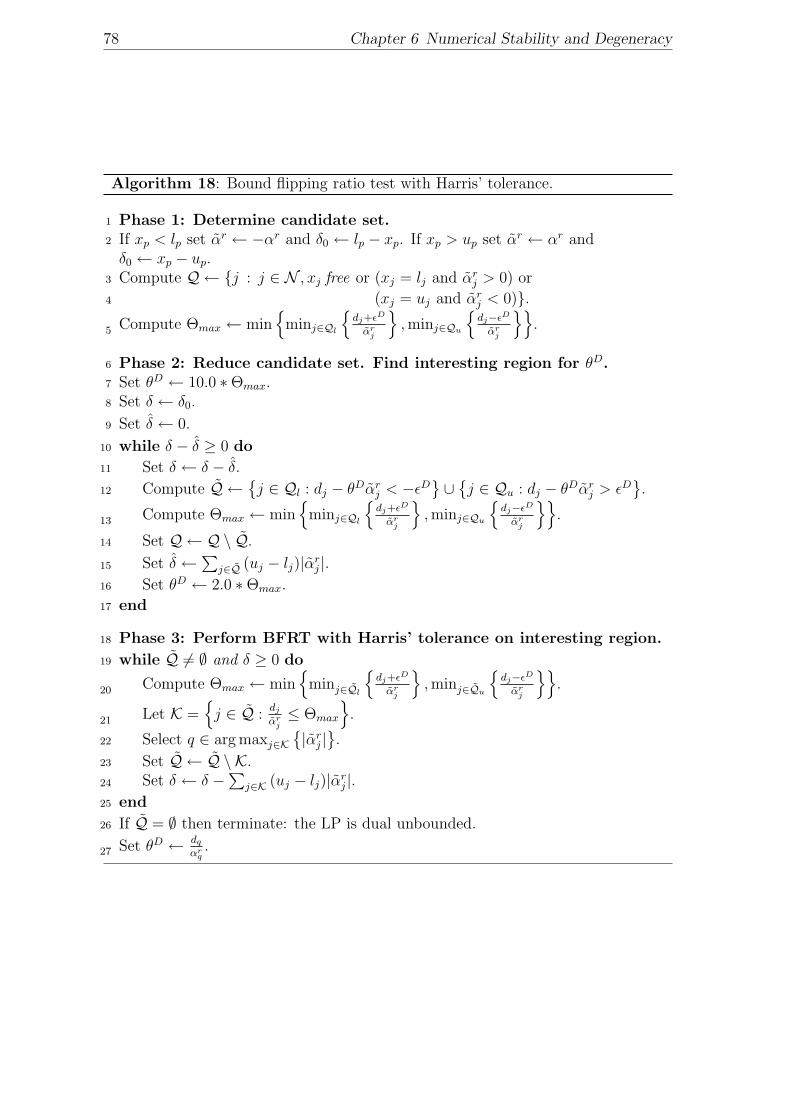
78 Chapter 6 Numerical Stability and Degeneracy
Algorithm 18: Bound flipping ratio test with Harris’ tolerance.
Phase 1: Determine candidate set.1
If xp < lp set αr ← −αr and δ0 ← lp − xp. If xp > up set αr ← αr and2
δ0 ← xp − up.Compute Q ← {j : j ∈ N , xj free or (xj = lj and αr
j > 0) or3
(xj = uj and αrj < 0)}.4
Compute Θmax ← min{
minj∈Ql
{dj+εD
αrj
},minj∈Qu
{dj−εD
αrj
}}.5
Phase 2: Reduce candidate set. Find interesting region for θD.6
Set θD ← 10.0 ∗Θmax.7
Set δ ← δ0.8
Set δ ← 0.9
while δ − δ ≥ 0 do10
Set δ ← δ − δ.11
Compute Q ←{j ∈ Ql : dj − θDαr
j < −εD}∪{j ∈ Qu : dj − θDαr
j > εD}.12
Compute Θmax ← min{
minj∈Ql
{dj+εD
αrj
},minj∈Qu
{dj−εD
αrj
}}.13
Set Q ← Q \ Q.14
Set δ ←∑
j∈Q (uj − lj)|αrj |.15
Set θD ← 2.0 ∗Θmax.16
end17
Phase 3: Perform BFRT with Harris’ tolerance on interesting region.18
while Q 6= ∅ and δ ≥ 0 do19
Compute Θmax ← min{
minj∈Ql
{dj+εD
αrj
},minj∈Qu
{dj−εD
αrj
}}.20
Let K ={j ∈ Q :
dj
αrj≤ Θmax
}.21
Select q ∈ arg maxj∈K{|αr
j |}.22
Set Q ← Q \ K.23
Set δ ← δ −∑
j∈K (uj − lj)|αrj |.24
end25
If Q = ∅ then terminate: the LP is dual unbounded.26
Set θD ← dq
αrq.27
6.2 Techniques to ensure numerical stability 79
for φ. A semi-rigorous analysis (for PFI) for this approach can be found in [15,p. 112f.]). For LU-factorization and update φ = 100 has turned out to be areasonable value. Fine-tuning for special problem classes is left to the user.
2. Dynamic frequency: φ is dynamically changed during the solution run. Inan analysis conducted by [75, p. 85f.] he assumes that the times T0 and Ti
mainly depend on the number of nonzero elements in the current basis matrixand the updated LU-representation, respectively. By simple bookkeeping hekeeps track of the quantities T ∗r and triggers a refactorization, when they startincreasing.
In our implementation we made good experiences with the simpler constant refac-torization frequency. We use a slightly modified variant, where we incorporate thenumber of rows m in the determination of φ in the following way:
φ = min{
100 +m
200, 2000
}. (6.26)
The constants in (6.26) are dependent on the system architecture and individualcharacteristics of the code and have been determined by extensive benchmarking.The reason to choose a higher refactorization frequency for models with many rowsis, that the time for refactorization shows a greater dependency on the number of rowsthan the solution times for FTran and BTran, especially for hypersparse problems.
6.2.3.2 Refactorization for stability
In every LU-update the numerical accuracy of the LU-factors decreases due to theaccumulation of small errors caused by the limited precision arithmetic. The degreeof accumulation and amplification depends on the condition number of the basismatrix, which may worsen in basis changes with small pivot elements (< 10−4 usuallycauses problems). For numerically easy problems (e.g. those with 0/1 problemmatrices and well modeled problems) both of these threads are irrelevant and noadditional refactorizations are necessary. For some problems, especially those whichare badly modeled, significant errors can occur, which in most cases can be fixed oreven prevented by a precocious refactorization and recomputation of the primal anddual basic solution. In the following we give a list of computationally cheap accuracychecks and ”numerical events”, which can be used to monitor the numerical statusof a solution run:
• Pivot element test. After the FTran operation in step 7 of elaborated dualsimplex method (algorithm 7), two versions of the pivot element αr
q are avail-able. The first version, which we will denote by αBT , is the q-th entry of thetransformed pivot row, which was computed in step 7:
αBT = (ATNρr)q. (6.27)
The second version denoted by αFT is the r-th entry of the transformed pivot
80 Chapter 6 Numerical Stability and Degeneracy
column computed in step 7:
αFT = (B−1aq)r (6.28)
If the deviation |αBT −αFT | of these two quantities exceeds a certain thresholdεs, a refactorization is triggered. In our code we set
εs = 10−9 ∗ (1 + |αFT |) (6.29)
In general, αFT can be assumed to be numerically more precise than αBT ,since besides the FTran operation no additional computations are involved.Therefore, one option in implementation is to always proceed with αFT afterFTran and to (re-)compute the primal and dual step length. While the updateof the primal and dual basic solution vectors can be performed with greateraccuracy in this case, the new dual step length might slightly differ from thevalue assumed in the dual ratio test. This can lead to the (uncontrolled) lossof dual feasibility, since it clearly counteracts the shifting policy in the dualratio test. Therefore, we keep using αBT in spite of its potential numericalweaknesses4.
• LU-update test. We already described this accuracy check in section 5.3.1as a feature of the Forrest/Tomlin update procedure. If
|αrq −
umm
utt
| > εu (6.30)
the basis change is aborted and a refactorization is triggered. To prevent arepetition the selected leaving variable is excluded from pricing for a certainnumber of iterations. In our code we set
εu = 10−6 · |αrq|. (6.31)
• DSE weight test. As mentioned in section 3.3 the dual steepest weight βr
corresponding to the leaving variable can be recomputed from its definitionat low costs since the r-th row of the basis matrix is readily available froma previous step of the algorithm (computation of the transformed pivot row).Let
βUr = βr and (6.32a)
βRr = ρT
r ρr (6.32b)
be the updated and the recomputed version of βr, respectively. Due to thehigher accuracy it is advisable to always replace βr by βR
r . Furthermore, thedeviation between these two version of βr can be used to get an impression ofthe current accuracy of the DSE weights, which can have great impact on theeffectiveness of DSE pricing (bad accuracy can lead to a significant increase
4In the remainder of this text we always assume that αrq = αBT .
6.2 Techniques to ensure numerical stability 81
of the total number of iterations). We do not use this test as a trigger forrefactorization or even recomputation of all DSE weights from their definition(usually is very expensive), but as a tool in development and debugging toimprove the general numerical behavior of our code.
• Reduced cost test. For the reduced cost value dq associated with the enteringvariable q the following is true:
dq = cq − yTaq = cq − cTBB−1aq = cq − cTBαq. (6.33)
Therefore, dq can be recomputed using the transformed pivot column αq afterthe FTran operation in step 7 of algorithm 7. The recomputed version of dq isin general more accurate than the updated version. The deviation between thetwo versions can be used to measure the accuracy of the reduced cost vectord. If it exceeds a certain threshold (e.g. 10−9), the recomputation of the dualbasic solution from its definition or a refactorization can be triggered. As in thepivot element test one could also replace dq by the recomputed, more accuratevalue. However, the induced change in the dual step length can lead to dualinfeasibilities and counteract the shifting strategy in the dual ratio test. In thelatest version we use this test merely as a tool in development and debugging.
• Primal and dual error. Let xB and y be the primal and dual basic solutionvectors resulting from the solution of the corresponding systems 2.13 and 2.15a.Then the (maximal) primal error errP and the (maximal) dual error errD aredefined as
errP = maxi∈{1,...,m}
{|(b−BxB)i|} and (6.34)
errD = maxi∈{1,...,m}
{|(cB −BT y)i|}. (6.35)
Computing errP and errD in this manner is rather expensive. Therefore weuse these measures only for development and debugging.
• Loss of feasibility. In spite of all precautions entries of the dual basic solu-tion can become dual infeasible beyond the dual infeasibility tolerance due tonumerical errors. It is important to incorporate adequate test to detect theseentries. In our code this is done in the dual ratio test. When a reduced costvalue is found to be dual infeasible the iteration is aborted, a refactorizationand a switch to the dual phase I is triggered.
82 Chapter 6 Numerical Stability and Degeneracy
6.3 Techniques to reduce degeneracy and preventcycling
6.3.1 Perturbation
As one can conclude from the definitions in section 2.4, degeneracy is in the firstinstance a property of a given LP problem. If most of the bases of an LP problemare degenerate by a high degree (dual, primal or both), the problem is said to behighly degenerate. Consequently, also the susceptibility to stalling is a property ofthe problem data. It is well known, that particularly the LP relaxations of combi-natorial optimization problems are often highly degenerate. The basic idea of theperturbation technique is to lower the amount of problem-inherent degeneracy byrandomly changing the problem data by small margins. Primal degeneracy can beresolved by perturbing the right-hand-side and/or the bounds of a problem. Dualdegeneracy can be resolved by perturbing the cost vector. In the following we willconsider only the latter.
Many variants of the perturbation method have been discussed in the literature.They differ with respect to the following points:
• When to perturb? Is the perturbation applied at the start of the methodor only when stalling occurs?
• What to perturb? Do we perturb only the cost coefficients of the degeneratepositions or all of them?
• How to perturb? Do we perturb by random quantities within a fixed intervalor do we consider the size of the cost coefficients or other measures?
• How to remove the perturbation? Do we remove the perturbations duringor only at the end of the solution run? Which method is used to remove them?
Our perturbation procedure, which is similar to the one implemented in the COINLP code [44], is applied prior to the dual simplex method, if many cost coefficientshave the same value. In fact, we sort the structural part of the cost vector andcount the number of different values. If this number is less then one fourth of thetotal number of structural variables, we assume the problem to be significantly dualdegenerate and perturb all structural non-fixed, non-free variables. If the problemwas not perturbed at the start and the objective function value does not improve forat least maxcycle iterations (we use maxcycle = 3 ·φ, where φ is the refactorizationfrequency), then we perturb only the degenerate positions of the above subset of thecost vector.
The determination of the cost changes is the main difference compared to othermethods from the literature. While these methods aim solely at resolving degeneracy,our perturbation procedure also tries to exploit degeneracy to keep the number ofnonzero elements in the basis matrix low. In general, the presence of degeneracyincreases the flexibility in the dual ratio test. If the problem is numerically stable,this flexibility can be used to select entering variables with as few nonzero elements
6.3 Techniques to reduce degeneracy and prevent cycling 83
in their corresponding columns of the problem matrix as possible. The effect is,that the spike in LU-update stays sparser and the number of nonzeros added to theLU-factorization lower. But if the problem is perturbed at the start, most of thisflexibility is lost5. Therefore, the number of nonzero elements is considered in thedetermination of the cost perturbations. The determination of a cost perturbationξj is performed in four steps:
1. Determine the right magnitude of ξj. Set ξj to a fixed value, which consistsof a constant fraction (typically 100 · εD) and a variable fraction dependent onthe size of the cost coefficient (typically ψ · cj, with ψ = 10−5).
2. Randomize ξj and set the right sign w.r.t. dual feasibility. This is done bysetting
ξj ←
{−0.5ξj(1 + µ) if uj <∞,
0.5ξj(1 + µ) o.w.,(6.36)
where µ is a random number within the interval [0, 1]. Note, that by usingequation (6.36) ξj basically keeps the size determined in step 1.
3. Incorporate nonzero counts. Dependent on the number νj of nonzero elementsin column aj, ξj is multiplied by a weighting factor wk:
ξj ← wνj· ξj. (6.37)
The weight-vector w displays the tradeoff between the two goals ”resolve de-generacy” and ”keep nonzero count low”. We use the following scheme:
wT = (10−2, 10−1, 1.0, 2.0, 5.0, 10.0, 20.0, 30.0, 40.0, 100.0). (6.38)
If νj > 10 we use w10 = 100.0 in equation (6.37). As mentioned before mostpractical LP problems have less than fifteen nonzero entries per column inde-pendent of the number of rows.
4. Ensure that ξj stays within an interval [ξmin, ξmax] with
ξmin = min{10−2εD, ψ} and (6.39)
ξmax = max{103εD, ψ · 10 · 1n
∑n
j=1cj}. (6.40)
If ξj exceeds or falls below these thresholds, it is multiplied with 0.1 or 10,respectively, until it falls into the above interval.
At the end of the dual simplex method we restore the original cost vector, whichcan lead to a loss of dual feasibility of the current basic solution. If the methodterminated due to primal feasibility, we switch to the primal simplex method (tobe more precise: primal phase II) to restore dual feasibility (cf. [9]). Usually, onlyfew iterations are necessary to find a new optimal basis. If the method terminated
5In this sense the perturbation also works against Harris’ ratio test.
84 Chapter 6 Numerical Stability and Degeneracy
due to dual unboundedness, we just restore the cost vector and start over with thedual phase I if necessary to confirm unboundedness. The same procedure is used toremove the cost shiftings performed in the dual ratio test.
6.3.2 Randomized pricing
It is well known that dual steepest edge pricing as described in section 3.3 is byitself an effective technique to reduce the number of degenerate iterations. Theleaving variable is determined by equation 3.53. While for most problems ties arerather unlikely, they occur with increased frequency on well conditioned LP problems,which are highly degenerate. One possible criterion to resolve a tie in dual pricingis the number of nonzero elements in the corresponding column of the U -part ofthe LU-factorization. However, we made better experiences with resolving the tiestotally randomly. On some problems this also lead to a dramatic reduction of (dual)degenerate iteration. Implementation details are given in sections 8.2.2.
85
Chapter 7
Further computational aspects
7.1 LP preprocessing, scaling and crash procedures
LP preprocessing, scaling and crash procedures are performed prior to the (dual)simplex algorithm. While preprocessing and scaling methods aim at improving themodel formulation given by the user, the crash procedure is supposed to quicklyobtain a starting basis which is superior to the all logical basis.
LP preprocessing
It is widely recognized that LP preprocessing is very important for solving large-scalelinear and integer optimization problems efficiently (cf. [14] and [49]). This is true forboth interior point and simplex algorithms. Although LP software and computershave become much faster, LP models have increased in size. Furthermore, LP opti-mizers are used in interactive applications and in integer programming where manyLP problems have to be solved. More efficient algorithms and improved implementa-tion techniques are therefore still very important. Furthermore all practical LP/IPmodels are generated by computer programs either directly or within a modelingsystem. The model generator derives the computer model from the mathematicalmodel structure and the model data. Most model generators have very limited ca-pabilities for data analysis. As a consequence, there is usually a significant part ofthe model that is redundant. The main goals of LP preprocessing are:
• eliminate as many redundant constraints as possible
• fix as many variables as possible
• transform bounds of single structural variables (either tightening / relaxingthem during LP preprocessing or tightening bounds during IP preprocessing)
• reduce the number of variables and constraints by eliminations
We refer here to the techniques described in [49]. The standard LP-preprocessingfor LPs to be solved with an interior point or primal simplex algorithm uses boundtightening in an early phase of the LP-preprocessing. At the end of LP-preprocessingthere is a reverse procedure where bounds are relaxed, i.e. redundant bounds areremoved from the model.
86 Chapter 7 Further computational aspects
As mentioned previously, boxed variables play a key role in the dual simplexalgorithm. Therefore tightened bounds are not relaxed if the dual simplex algorithmis used in our code. In chapter 9 we demonstrate the surprising impact of thisstrategy in our computational results.
Scaling
Scaling procedures try to decrease the numerical difficulty of a user given (or alreadypreprocessed) model by reducing the spread of magnitudes of nonzeros in the problemdata. This is done by multiplying the rows and columns of the constraint matrix withreal valued scaling factors. There are several methods in the literature to determinethese factors, surveys can be found in [73] and [46, p. 110ff.]. The method usedin MOPS was first presented in [9] and is implemented with minor modificationsdescribed in [65].
Crash
The purpose of a crash procedure is to find a good starting basis for the (dual)simplex method with the following properties:
1. Easy to factorize. The all logical basis is clearly the best choice with respect tothis requirement. However, it leaves no flexibility to take other considerationsinto account. Therefore, most crash procedures try to generate a triangular ornear triangular basis as a good compromise.
2. As feasible, optimal and sparse as possible. Ties in the triangulation proce-dure are resolved by a weight function preferring variables with a high primalfeasibility range and a low nonzero count in the corresponding column of theconstraint matrix. Free variables are tried to be pivoted into and fixed vari-ables out of the basis. The probability of a variable to be part of an optimalbasis is estimated by the objective function coefficient and simple geometricarguments (cf. [54]).
3. Numerically stable. As in the factorization procedure the threshold pivotingcriterion (cf. [23]) can be used to avoid the generation of an ill-conditionedbasis.
An overview of common crash procedures can be found in [46, p. 244ff.]. The methodincluded in the MOPS system is described in [65]. In the context of this dissertationwe did not change this procedure. However, we conducted some computational testswith the result that we could not achieve a significant performance improvementcompared to the all logical basis. One important reason is the increased density ofa crash basis, which leads to slower iterations in the beginning of a solution run andhas to be overcompensated by a reduction of the total iteration count. In the contextof the dual simplex method this is problematic due to the other important reason,which is dual steepest edge pricing. If we start the dual simplex method with anall logical basis, then the dual steepest edge weights βi can be initialized with 1.0,
7.2 Computation of the pivot row 87
which is the correct value with respect to their definition. For any other startingbasis, we can either keep this cheap initialization as a heuristic or compute the exactweights according to formula 3.45. This is computationally very expensive since itrequires the solution of up to m linear systems for ρi plus up to m inner products.Using crash and the simple initialization lead to disastrous results: both the totalnumber of iteration and the total solution time increased dramatically for almost allof the test models. Using the time consuming exact initialization was much morepromising. The total number of iterations could be reduced significantly in manycases. However, this saving did not compensate the additional effort for most of thetest models. Therefore, our default is not to use a crash basis for the dual simplexin MOPS.
7.2 Computation of the pivot row
The computation of the pivot row αr (step 7 of algorithm 7) is one of the most timeconsuming operations of the dual simplex method. For some models it can take morethan 50% of the total solution time (cf. [11]) even for sophisticated implementations.Therefore, this step has to be implemented with great care.
To begin with we recall that the problem data complies with the internal modelrepresentation described in (2.3). From the definition of αr we can directly conclude,that
αrj = ρj−n
r if j > n. (7.1)
Thus no computation is necessary at all for columns corresponding to logical vari-ables.
In principle, the structural part of αr can be computed in two different ways.Using columnwise computation the entries αr
j are computed independently by theinner product
αrj = ρr
Taj =∑
i∈I(aj)
ρira
ij, (7.2)
where I(aj) denotes the set of row indices of nonzero elements in column aj. Inequation (7.2) we can exploit sparsity of AN by using the columnwise compact storageof A, which is available anyway. Basic and fixed variables can easily be skipped. It isalso easy to build up an index stack for those nonzero elements of αr, which exceedthe zero tolerance εz. The disadvantage of the columnwise computation is, that thesparsity of ρr cannot be exploited.
In the rowwise computation αr is calculated as follows:
αr = ATNρr =
∑i∈I(ρr)
ρira
iN , (7.3)
where aiN denotes the i-th row of AN . Sparsity of AN can be exploited by using
a rowwise compact storage of A to calculate the product ρira
iN . This needs to be
done only for nonzero positions of ρr, which can drastically reduce the computationaleffort, especially for hypersparse models.
88 Chapter 7 Further computational aspects
However, the rowwise computation also has some disadvantages. The need foran additional rowwise datastructure for A significantly increases the memory re-quirements of the method. Furthermore, positions of αr corresponding to basic orfixed variables cannot easily be skipped. In [11] Bixby recommends to maintain arowwise data structure only for nonbasic nonfixed positions and update it in everybasis change. Inserting a column into the data structure is usually very cheap, sincethe time required per nonzero element is constant. But for deleting a column thistime is linear in the number of nonzeros of the affected row, so this operation canbe quite expensive. In fact, in our tests we made bad experiences for models withmany more columns than rows. On the other hand we could not see a significantspeedup compared to the version without updating, so we decided to use a completerowwise storage of A in our implementation. When the dual simplex method is usedas a part of a branch-and-cut procedure for mixed-integer programming this datastructure has to be derived anyway for other purposes. A further disadvantage of therowwise computation is, that the build-up of an index stack requires an additionalpass over the nonzero elements, since αr has to be hold in a dense array to calculatethe sum in equation (7.3). For these reasons, we use both the columnwise and therowwise computation dependent on the density of ρr. If it exceeds 30% then thecolumnwise computation is used. For models with a many more columns than rowsthis threshold is lowered to 10%.
Finally we want to mention an interesting idea brought to our mind by P.Q.Pan in personal conversation, which could be named partial ratio test. In a first passonly those nonbasic nonfixed positions of the transformed pivot row are computed forwhich the corresponding reduced cost entry is zero. As soon as one of these positionsdefines a breakpoint (αr
j nonzero and of right sign), it is taken as the entering variable.In this case the iteration must be degenerate and the further computation of thetransformed pivot row as well as the dual ratio test and the update of the reducedcost vector can be skipped. Pan reports a significant improvement of his code bythis idea. Up to now, we have not tested this technique, since it obviously collideswith several other concepts in our code, as the bound flipping ratio test, the costshifting scheme and the perturbation.

89
Part III
Implementation and results


91
Chapter 8
Implementation
8.1 The Mathematical OPtimization System MOPS
8.1.1 MOPS and its history
MOPS1 is a high performance Mathematical Programming Software System for solv-ing large-scale LP and mixed integer optimization problems (MIPs), which has chieflybeen developed by U. Suhl since the year 1987. The system is written in FOR-TRAN77 and has been ported to various popular system platforms ranging fromWindows PCs and servers to mainframes. It has been deployed in many practicalapplications for over two decades (see e.g. [69], [67], [62] and [37]) and has con-tinuously been improved in algorithms, software design and implementation (seetable 8.1). The system started as a pure LP-solver based on a high speed primalsimplex algorithm. In its present form MOPS also features powerful dual simplex andinterior point engines, as well as an effective branch-and-cut procedure. It belongsto the few competitive systems in the world to solve large-scale linear and mixedinteger programming problems. The algorithms and computational techniques usedin MOPS have been documented in several scientific publications
• on the primal simplex and system architecture [65, 66],
• on the LU-factorization [68] and LU-Update [63],
• LP-preprocessing [70, 49],
• super node processing [71],
• and on the dual simplex algorithm [38] and dual phase I [39].
The algorithmic improvements in the LP as well as in the IP part of MOPS canbe seen by considering the solution times of the benchmark model oil, which is smallby today’s standard. The model has 5563 constraints, 6181 structural variables, 74are 0-1 variables and 39597 nonzeros in the coefficient matrix. Tables 8.2 and 8.3show the improvements for LP- and IP-optimization on oil, respectively.
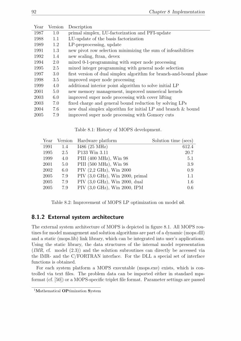
92 Chapter 8 Implementation
Year Version Description1987 1.0 primal simplex, LU-factorization and PFI-update1988 1.1 LU-update of the basis factorization1989 1.2 LP-preprocessing, update1991 1.3 new pivot row selection minimizing the sum of infeasibilities1992 1.4 new scaling, ftran, devex1994 2.0 mixed 0-1-programming with super node processing1995 2.5 mixed integer programming with general node selection1997 3.0 first version of dual simplex algorithm for branch-and-bound phase1998 3.5 improved super node processing1999 4.0 additional interior point algorithm to solve initial LP2001 5.0 new memory management, improved numerical kernels2003 6.0 improved super node processing with cover lifting2003 7.0 fixed charge and general bound reduction by solving LPs2004 7.6 new dual simplex algorithm for initial LP and branch & bound2005 7.9 improved super node processing with Gomory cuts
Table 8.1: History of MOPS development.
Year Version Hardware platform Solution time (secs)1991 1.4 I486 (25 MHz) 612.41995 2.5 P133 Win 3.11 20.71999 4.0 PIII (400 MHz), Win 98 5.12001 5.0 PIII (500 MHz), Win 98 3.92002 6.0 PIV (2,2 GHz), Win 2000 0.92005 7.9 PIV (3,0 GHz), Win 2000, primal 1.12005 7.9 PIV (3,0 GHz), Win 2000, dual 1.62005 7.9 PIV (3,0 GHz), Win 2000, IPM 0.6
Table 8.2: Improvement of MOPS LP optimization on model oil.
8.1.2 External system architecture
The external system architecture of MOPS is depicted in figure 8.1. All MOPS rou-tines for model management and solution algorithms are part of a dynamic (mops.dll)and a static (mops.lib) link library, which can be integrated into user’s applications.Using the static library, the data structures of the internal model representation(IMR, cf. model (2.3)) and the solution subroutines can directly be accessed viathe IMR- and the C/FORTRAN interface. For the DLL a special set of interfacefunctions is obtained.
For each system platform a MOPS executable (mops.exe) exists, which is con-trolled via text files. The problem data can be imported either in standard mps-format (cf. [50]) or a MOPS-specific triplet file format. Parameter settings are passed
1Mathematical OPtimization System
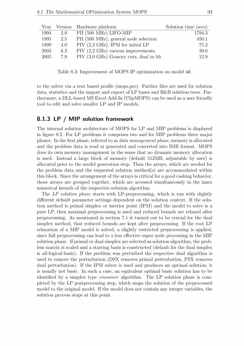
8.1 The Mathematical OPtimization System MOPS 93
Year Version Hardware platform Solution time (secs)1994 2.0 PII (500 MHz) LIFO-MIP 1794.31995 2.5 PII (500 MHz), general node selection 450.11999 4.0 PIV (2,2 GHz), IPM for initial LP 75.22003 6.3 PIV (2,2 GHz) various improvements 39.62005 7.9 PIV (3,0 GHz) Gomory cuts, dual in bb 12.9
Table 8.3: Improvement of MOPS IP optimization on model oil.
to the solver via a text based profile (mops.pro). Further files are used for solutiondata, statistics and the import and export of LP bases and B&B solution trees. Fur-thermore, a DLL-based MS Excel Add-In (ClipMOPS) can be used as a user friendlytool to edit and solve smaller LP and IP models.
8.1.3 LP / MIP solution framework
The internal solution architecture of MOPS for LP and MIP problems is displayedin figure 8.2. For LP problems it comprises two and for MIP problems three majorphases. In the first phase, referred to as data management phase, memory is allocatedand the problem data is read or generated and converted into IMR format. MOPSdoes its own memory management in the sense that no dynamic memory allocationis used. Instead a large block of memory (default 512MB, adjustable by user) isallocated prior to the model generation step. Then the arrays, which are needed forthe problem data and the requested solution method(s) are accommodated withinthis block. Since the arrangement of the arrays is critical for a good cashing behavior,those arrays are grouped together, which are accessed simultaneously in the innernumerical kernels of the respective solution algorithm.
The LP solution phase starts with LP-preprocessing, which is run with slightlydifferent default parameter settings dependent on the solution context. If the solu-tion method is primal simplex or interior point (IPM) and the model to solve is apure LP, then maximal preprocessing is used and reduced bounds are relaxed afterpreprocessing. As mentioned in section 7.1 it turned out to be crucial for the dualsimplex method, that reduced bounds are kept after preprocessing. If the root LPrelaxation of a MIP model is solved, a slightly restricted preprocessing is applied,since full preprocessing can lead to a less effective super node processing in the MIPsolution phase. If primal or dual simplex are selected as solution algorithm, the prob-lem matrix is scaled and a starting basis is constructed (default for the dual simplexis all-logical-basis). If the problem was perturbed the respective dual algorithm isused to remove the perturbation (DSX removes primal pertrubation, PSX removesdual perturbation). If the IPM solver is used and produces an optimal solution, itis usually not basic. In such a case, an equivalent optimal basic solution has to beidentified by a simplex type crossover algorithm. The LP solution phase is com-pleted by the LP postprocessing step, which maps the solution of the preprocessedmodel to the original model. If the model does not contain any integer variables, thesolution process stops at this point.
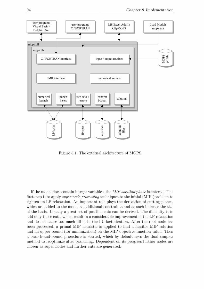
94 Chapter 8 Implementation
mops.dll
mops.lib
user programsVisual Basic / Delphi / .Net
C / FORTRAN interface
Load Modulemops.exe
MS Excel Add-InClipMOPS
user programsC / FORTRAN
numerical kernelsIMR interface
input / output routines
numerical kernels solutionconvert
bcdouttree save /
restorepunchinsert
MO
PS
prof
ile
solu
tion
files
mps
dat
a
IP tr
ees
LP b
ases
Figure 8.1: The external architecture of MOPS
If the model does contain integer variables, the MIP solution phase is entered. Thefirst step is to apply super node processing techniques to the initial (MIP-)problem totighten its LP relaxation. An important role plays the derivation of cutting planes,which are added to the model as additional constraints and as such increase the sizeof the basis. Usually a great set of possible cuts can be derived. The difficulty is toadd only those cuts, which result in a considerable improvement of the LP relaxationand do not cause too much fill-in in the LU-factorization. After the root node hasbeen processed, a primal MIP heuristic is applied to find a feasible MIP solutionand an upper bound (for minimization) on the MIP objective function value. Thena branch-and-bound procedure is started, which by default uses the dual simplexmethod to reoptimize after branching. Dependent on its progress further nodes arechosen as super nodes and further cuts are generated.
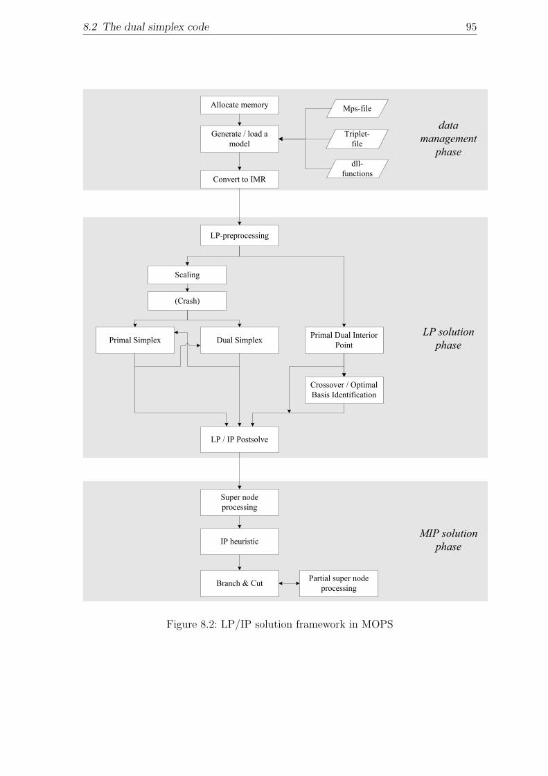
8.2 The dual simplex code 95
Allocate memory
Generate / load a model
Scaling
LP / IP Postsolve
(Crash)
Convert to IMR
LP-preprocessing
Mps-file
dll-functions
Triplet-file
Primal Dual Interior Point
IP heuristic
Super node processing
Crossover / Optimal Basis Identification
Branch & Cut Partial super node processing
Primal Simplex
data management
phase
MIP solution phase
LP solution phaseDual Simplex
Figure 8.2: LP/IP solution framework in MOPS
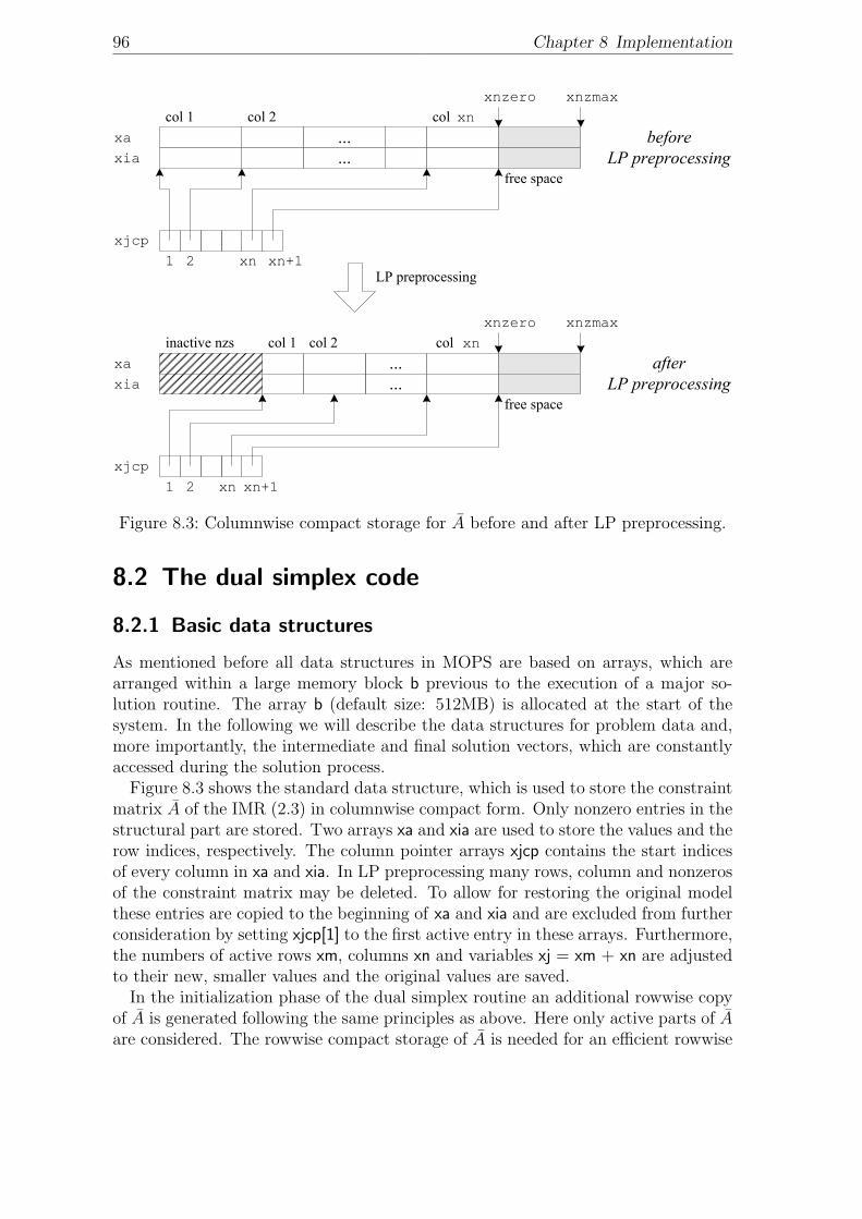
96 Chapter 8 Implementation
...
...xaxia
xjcp
col 1 col 2 col xnxnzero xnzmax
free space
1 2 xn xn+1
...
...xaxia
xjcp
col 1 col 2xnzero xnzmax
free space
1 2 xn xn+1
inactive nzs col xn
LP preprocessing
before LP preprocessing
after LP preprocessing
Figure 8.3: Columnwise compact storage for A before and after LP preprocessing.
8.2 The dual simplex code
8.2.1 Basic data structures
As mentioned before all data structures in MOPS are based on arrays, which arearranged within a large memory block b previous to the execution of a major so-lution routine. The array b (default size: 512MB) is allocated at the start of thesystem. In the following we will describe the data structures for problem data and,more importantly, the intermediate and final solution vectors, which are constantlyaccessed during the solution process.
Figure 8.3 shows the standard data structure, which is used to store the constraintmatrix A of the IMR (2.3) in columnwise compact form. Only nonzero entries in thestructural part are stored. Two arrays xa and xia are used to store the values and therow indices, respectively. The column pointer arrays xjcp contains the start indicesof every column in xa and xia. In LP preprocessing many rows, column and nonzerosof the constraint matrix may be deleted. To allow for restoring the original modelthese entries are copied to the beginning of xa and xia and are excluded from furtherconsideration by setting xjcp[1] to the first active entry in these arrays. Furthermore,the numbers of active rows xm, columns xn and variables xj = xm + xn are adjustedto their new, smaller values and the original values are saved.
In the initialization phase of the dual simplex routine an additional rowwise copyof A is generated following the same principles as above. Here only active parts of Aare considered. The rowwise compact storage of A is needed for an efficient rowwise
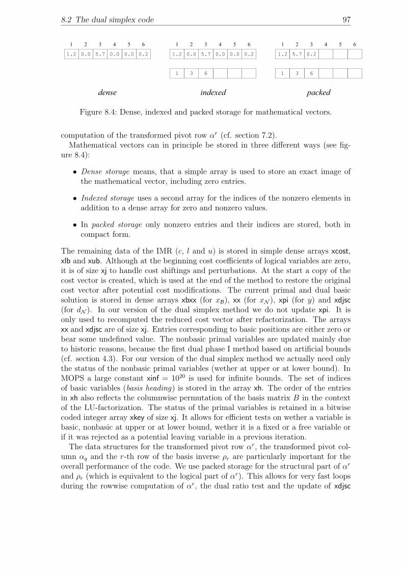
8.2 The dual simplex code 97
1.2 0.20.00.05.70.0
1 65432
1.2 0.25.7
1 65432
1.2 0.20.00.05.70.0
1 65432
1 631 63
dense packedindexed
Figure 8.4: Dense, indexed and packed storage for mathematical vectors.
computation of the transformed pivot row αr (cf. section 7.2).Mathematical vectors can in principle be stored in three different ways (see fig-
ure 8.4):
• Dense storage means, that a simple array is used to store an exact image ofthe mathematical vector, including zero entries.
• Indexed storage uses a second array for the indices of the nonzero elements inaddition to a dense array for zero and nonzero values.
• In packed storage only nonzero entries and their indices are stored, both incompact form.
The remaining data of the IMR (c, l and u) is stored in simple dense arrays xcost,xlb and xub. Although at the beginning cost coefficients of logical variables are zero,it is of size xj to handle cost shiftings and perturbations. At the start a copy of thecost vector is created, which is used at the end of the method to restore the originalcost vector after potential cost modifications. The current primal and dual basicsolution is stored in dense arrays xbxx (for xB), xx (for xN ), xpi (for y) and xdjsc(for dN ). In our version of the dual simplex method we do not update xpi. It isonly used to recomputed the reduced cost vector after refactorization. The arraysxx and xdjsc are of size xj. Entries corresponding to basic positions are either zero orbear some undefined value. The nonbasic primal variables are updated mainly dueto historic reasons, because the first dual phase I method based on artificial bounds(cf. section 4.3). For our version of the dual simplex method we actually need onlythe status of the nonbasic primal variables (wether at upper or at lower bound). InMOPS a large constant xinf = 1020 is used for infinite bounds. The set of indicesof basic variables (basis heading) is stored in the array xh. The order of the entriesin xh also reflects the columnwise permutation of the basis matrix B in the contextof the LU-factorization. The status of the primal variables is retained in a bitwisecoded integer array xkey of size xj. It allows for efficient tests on wether a variable isbasic, nonbasic at upper or at lower bound, wether it is a fixed or a free variable orif it was rejected as a potential leaving variable in a previous iteration.
The data structures for the transformed pivot row αr, the transformed pivot col-umn αq and the r-th row of the basis inverse ρr are particularly important for theoverall performance of the code. We use packed storage for the structural part of αr
and ρr (which is equivalent to the logical part of αr). This allows for very fast loopsduring the rowwise computation of αr, the dual ratio test and the update of xdjsc
98 Chapter 8 Implementation
if αr and ρr are sparse. This is especially the case for large hypersparse problems.While ρr is usually also sparse on typical medium sized and small problems, thestructural part of αr can get fairly dense. For these problems, where the density ofαr often exceeds 40% dense storage would pay off. To avoid further complication ofthe code, we decided to pass on this option for now.
The input and output vectors of our FTran and BTran routines are all in indexedstorage. Consequently, we need a loop over the nonzero elements of ρr after theBTran operation in step 7 to create the packed format. However, we also keep thedense representation of ρr. This is needed as an input for the FTran operation in thecontext of the update of the DSE weights and might be needed for the columnwisecomputation of αr. For the transformed pivot column αq we use indexed storage,which is readily obtained by the FTran operation in step 7. We decide upon thedensity of αq, wether we use the corresponding index array during the update ofxbxx and the DSE weights, which are stored in a dense array xbeta. If it exceeds30%, we use dense processing2.
While the packed arrays are overwritten in every iteration, the dense arrays forρr and αq have to be zero at the beginning of every iteration. We use the indexarrays to zero out the dense arrays after each iteration, which is crucial especiallyfor hypersparse problems (the careful organization of this clearing operation alonesaved about 15% of runtime on the large hypersparse NetLib model ken-18).
8.2.2 Pricing
As described in section 3.3, we use dual steepest edge pricing (DSE) based on themethod called ”Dual Algorithm I” by Forrest and Goldfarb [26] to select a variableto leave the basis. Three tasks have to be covered to implement this strategy:
1. (Re-)Initialization of the vector of DSE weights.
2. Update of the DSE weights.
3. Efficient selection of a leaving variable by passing through the weighted primalinfeasibilities.
During the development process of our code we learned that the way each of thesethree tasks is implemented has a great impact on the performance of the code. In thefollowing we will discuss the issues, that made a difference in our implementation.
8.2.2.1 Initialization and update of DSE weights
As mentioned before the DSE pricing strategy ”Dual Algorithm I” can be viewedas a heuristic itself, since it does not guarantee that actually the leaving variablecorresponding to the steepest edge is selected if boxed variables are present. Never-theless, we learned from the work with our code that the DSE weights have to be
2This entails that the code for the respective update routines practically doubles: one versionloops over the index array, the other version loops over xm.
8.2 The dual simplex code 99
initialized and updated with greatest possible accuracy. Even small errors can leadto a substantial increase of the iteration count.
The update is conducted according to equations (3.47a) and (3.50). At first werecompute the value of the weight βr = ρT
r ρr by its definition using the indexedstorage of ρr. Since βr is used in the update of all other weights, spending this extraeffort is worthwhile to avoid accumulation of errors. In debugging mode we also testthe numerical accuracy of βr at this point by comparing the recomputed value withthe updated version. To obtain the updated value βr according to equation (3.47a)βr has to be divided by the square of the pivot element αr
q. In the context of theDSE update we use the FTran version of it instead of the BTran version, since itis generally of higher numerical precision (cf. section 6.2.3.2). Next we perform theFTran operation on ρr to obtain the vector τ according to equation (3.49) and startthe update loop for the remaining weights. If αq is sparse we only loop over itsnonzero positions using the associated index vector.
In our very first DSE implementation we computed the update formula for the βi
exactly as it is stated in equation (3.50). We then tested the following reorganizedform (it is easy to see, that it is equivalent to (3.50)):
βi = βi + αiq
(αi
qβr + κτi)
with κ =−2
αrq
. (8.1)
In both cases we avoid negative weights by setting βi = max{βi, 10−4} as recom-mended in [26]. On most models (8.1) worked substantially better than the originalversion. The reason is clear: it avoids to square αi
q right away but performs thedivision first. Therefore, smaller values are involved in the computations, which re-duces the numerical error. We were surprised that the numerical accuracy of theDSE weights had such great impact on their efficacy.
This was confirmed by testing several variants of initializing the weights. Comput-ing the weights from their definition for an arbitrary basis is very expensive (up tom BTran operations). For an all-logical basis we know that 1.0 is the correct initialvalue. But even if we start with an all logical basis, it may change substantiallyduring the dual phase I, where we do not necessarily apply DSE pricing at all (e.g.in Pan’s dual phase I, cf. section 4.5). Furthermore, due to the permutation of thebasis after each refactorization, the vector of DSE weights becomes invalid. Due tothese considerations we just reset the weights to 1.0 after every refactorization in anearly version of our code. Later, we changed this simple strategy as follows:
• If no crash is used we initialize the weights with 1.0, otherwise (with crash) wedo the expensive initialization from their definition (BTran is only necessaryfor rows, which are not unit vectors).
• Prior to each refactorization the weights are copied to a dense vector of lengthxj in such a way that weight βi is assigned to the position corresponding to theindex B(i) of the associated basic variable. After the factorization the weightsare reassigned taking into account the new permutation of the basis.
• To have the correct values in dual phase II, the weights are always updated in
100 Chapter 8 Implementation
dual phase I, even if they are not used (e.g. in Pan’s phase I algorithm).
• During the update of the weights we save the old values of the weights thatare changed in a packed array. If an iteration is aborted after the weights havealready been updated, we use this array to restore the original values. Thissituation can occur if the stability test in LU-update fails.
With these changes we achieved a great improvement compared to the simpler imple-mentation. A crashed starting bases lead to a reduction of the total iteration countonly if the DSE weights were correctly initialized. However, even then runtime didnot improve in most of the cases, since the average time per iteration increased.
If the dual simplex method is deployed to reoptimize during branch-and-bound,there is no time to recompute the weights in every node of the B&B tree. Here, thedefault is to reuse the weights of the last LP-iteration.
8.2.2.2 Vector of primal infeasibilities
In the actual pricing step 7 we have to loop through the weighted primal infeasibilitiesto select the leaving variable. In the first version of our code we just implemented asimple loop over the primal basic variables following equation 3.53. Primal feasibilitywas tested within this loop.
Typically, 20–40% of the primal basic variables are infeasible at the start. Forsome problems this fraction is even lower. During the solution process the number ofinfeasibilities usually decreases continuously, until the basis is finally primal feasible.To exploit this observation, we changed our code to maintain an explicit indexedvector of the primal infeasibilities3. In the following xpifs denotes the dense arrayof the squared infeasibilities and xpifsi denotes the corresponding index array. Thisdata structure is renewed after each recomputation (after each refactorization) andadjusted during the update of the primal basic solution xB. Four cases can occur inthe update of a primal basic variable xB(i):
1. xB(i) stays primal feasible. The vector of primal infeasibilities does not change.
2. xB(i) becomes primal infeasible. The squared infeasibility is recorded in xpifsand the index i is added to xpifsi, which length increases by one.
3. xB(i) becomes primal feasible. The i-th entry of xpifs is replaced by a smallconstant 10−50 to signal feasibility. xpifsi is not changed.
4. xB(i) stays primal infeasible. xpifs[i] is adjusted. xpifsi is not changed.
Typically, the number of indices stored in xpifsi increases moderately between tworefactorizations and drops down to the actual number of infeasibilities after the nextrecomputation of xB. Using this vector of infeasibilities lead to great improvements ofruntime especially on large models. But also on many smaller problems considerablesavings could be achieved.
3Actually, the squared infeasibilities (distances to the respective bounds) are stored to furtherspeed up the DSE pricing loop.
8.2 The dual simplex code 101
8.2.2.3 Partial randomized pricing
On large easy problems the computational effort spent in the pricing loop can befurther reduced by considering only a small fraction φ of the infeasible positions.Only if all of these positions are actually feasible, further entries are examined toguarantee the selection of a leaving variable unless the basis is optimal. In eachiteration φ is dynamically adjusted within an interval of 1
20to 1 dependent on the
current relative iteration speed. As an estimate of the computational effort periteration we take a ratio of the number of nonzero elements in the LU-factors andthe number of rows xm. The default is φ = 1
8, which is decreased if the ratio drops
below a value of 2.0 and increased if it exceeds a value of 10.0.To give all primal infeasibilities the same probability to be considered we determine
a random starting point for the pricing loop. On some problems this randomizationof pricing also lead to fewer degenerate iteration. Furthermore, it reduces the risk ofnumerical cycling (cf. section 6.3.2).
8.2.3 Ratio test
Our implementation of the bound flipping ratio test (BFRT) is similar to the rou-tine ClpSimplexDual::dualColumn(. . . ) of the COIN LP Dual Simplex code [44]. Wealready gave an algorithmic description of this very sophisticated implementation insection 6.2.2.4 and algorithm 18. In this section we will discuss data structures andimplementation details.
The crucial issue of the implementation of the BFRT is, how the set Q of candi-date breakpoints is organized. Maros [47] and Fourer [27] recommend a heap datastructure for partially sorting the breakpoints, since it provides the best theoreticalcomplexity. The drawback of this approach is that a relatively expensive4 build-heapoperation has to be performed independently of the number of breakpoints, that canactually be passed.
Therefore, the COIN code follows a different path. After the set of breakpoints Qhas been determined in a first pass over the transformed pivot row (phase 1 in algo-rithm 18), this set is successively reduced to find a set of interesting breakpoints Q(phase 2 ). Only for these breakpoints the BFRT with Harris’ tolerance is performedin phase 3 as described in section 6.2.2.4.
The processing of the breakpoints in the three phases is depicted in figure 8.5. Itis organized by means of two packed vector data structures of length xj with valuearrays A[0] and A[1] and index arrays I[0] and I[1]. In phase 1, for every breakpointin Q the corresponding pivot row entry5 αr
j and the column index j is stored in A[0]and I[0], respectively. These breakpoints constitute the set Q1 in phase 2. In thefirst round of phase 2, temporary reduced cost values are computed for positionsin Q1 based on a first reasonable guess for the dual step length θD. If a positionstays dual feasible for this θD, it joins the set Q2 (the set of remaining breakpoints),which is stored at the beginning of the second packed vector (A[1] and I[1]). If aposition becomes dual infeasible for this θD, it joins the set Q1 (the set of possibly
4though the theoritical complexity bound is O(n)5actually αr
j
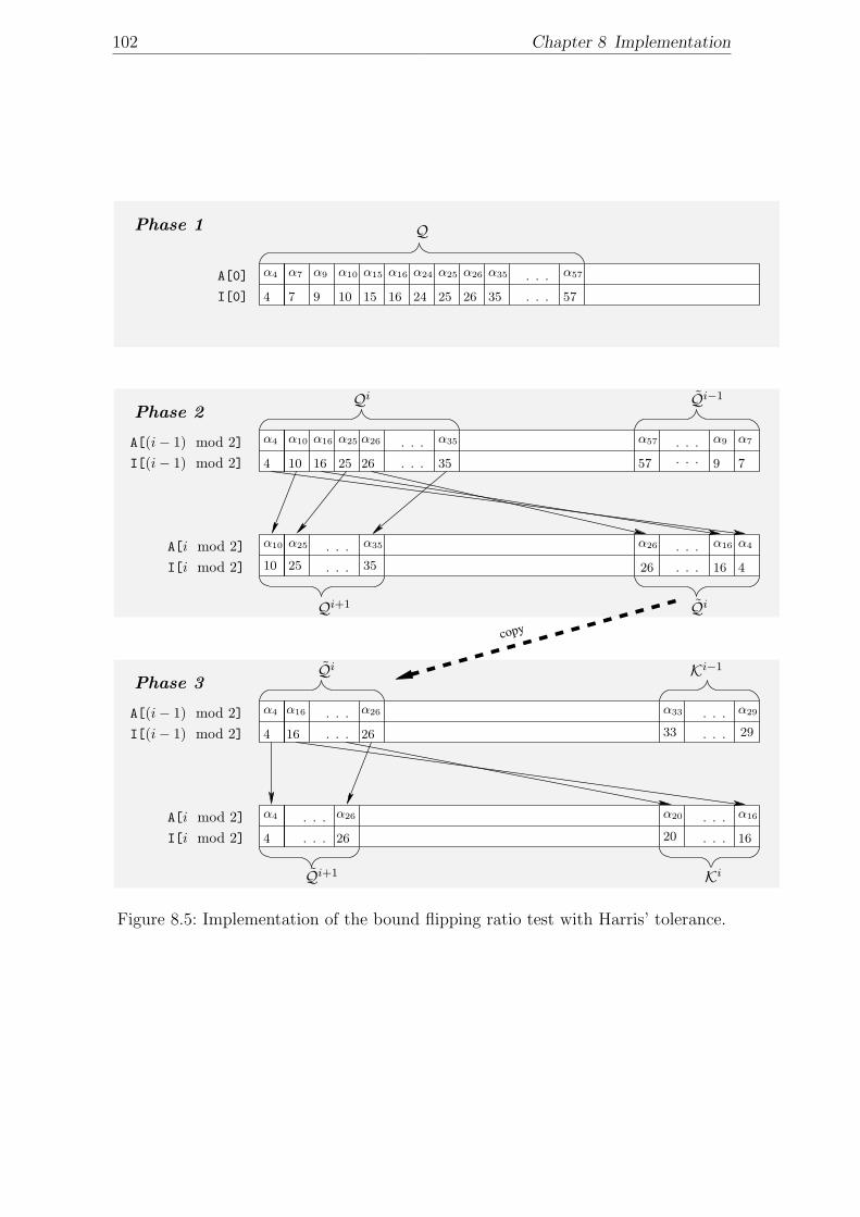
102 Chapter 8 Implementation
copy
I[i mod 2]A[i mod 2]
I[(i− 1) mod 2]A[(i− 1) mod 2]
Phase 3
I[i mod 2]A[i mod 2]
Phase 2
Phase 1
I[(i− 1) mod 2]A[(i− 1) mod 2]
I[0]
A[0]
Q
573526252416151097
. . .
. . .4
α57α35α26α25α24α16α15α10α9α7α4
. . .
. . .4
α4
α4
4
α16
16
α26
26
. . .
. . .
. . .
. . .
α29
2933
α33
Qi Ki−1
α16
16
α20
20
α26
26
. . .
. . .
Qi+1 Ki
α4 α10 α16 α25
4 . . .
. . .
10 16 25
Qi
α35
35
α57
57
α9
9
α7
7
Qi−1
. . .
. . .α26
26
. . .
. . .
. . .
. . .
α10
10
α25
25
α35
35
α4
4
α16
16
Qi+1 Qi
α26
26
Figure 8.5: Implementation of the bound flipping ratio test with Harris’ tolerance.
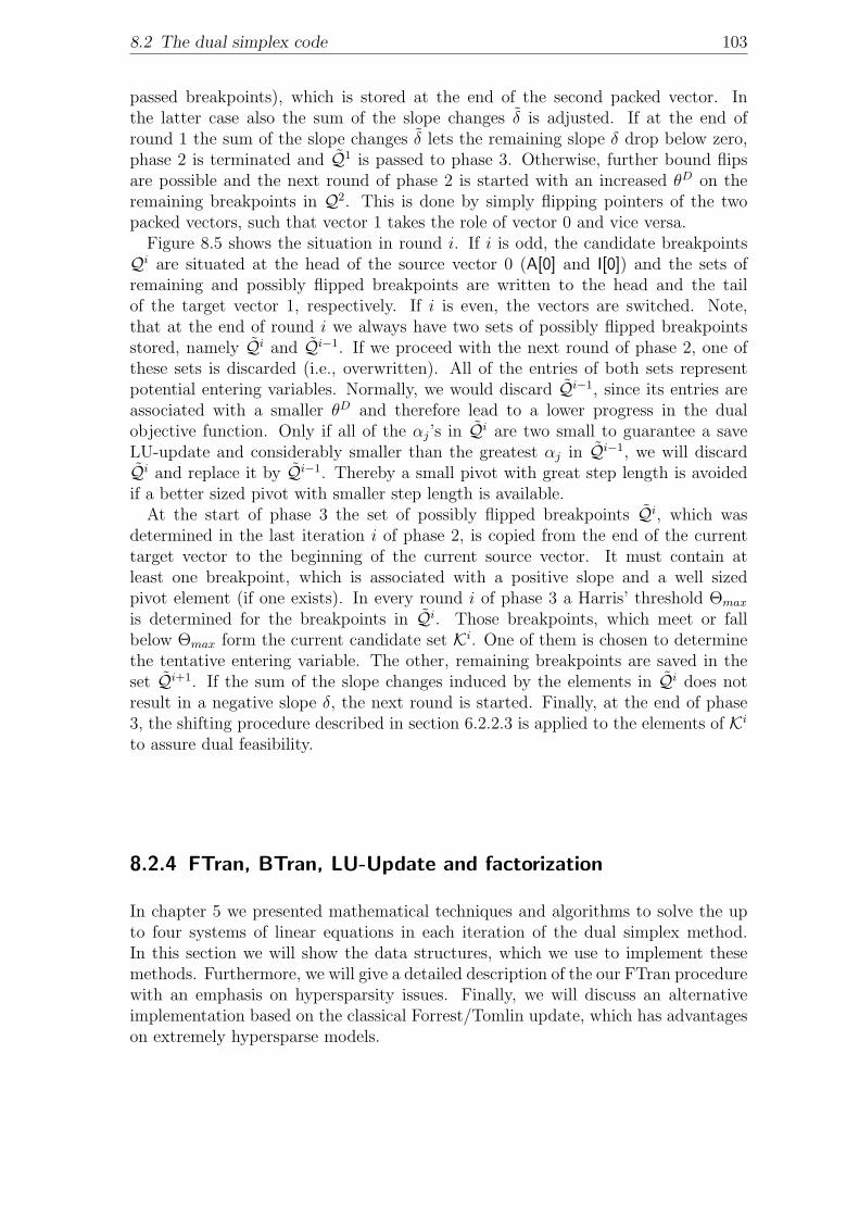
8.2 The dual simplex code 103
passed breakpoints), which is stored at the end of the second packed vector. Inthe latter case also the sum of the slope changes δ is adjusted. If at the end ofround 1 the sum of the slope changes δ lets the remaining slope δ drop below zero,phase 2 is terminated and Q1 is passed to phase 3. Otherwise, further bound flipsare possible and the next round of phase 2 is started with an increased θD on theremaining breakpoints in Q2. This is done by simply flipping pointers of the twopacked vectors, such that vector 1 takes the role of vector 0 and vice versa.
Figure 8.5 shows the situation in round i. If i is odd, the candidate breakpointsQi are situated at the head of the source vector 0 (A[0] and I[0]) and the sets ofremaining and possibly flipped breakpoints are written to the head and the tailof the target vector 1, respectively. If i is even, the vectors are switched. Note,that at the end of round i we always have two sets of possibly flipped breakpointsstored, namely Qi and Qi−1. If we proceed with the next round of phase 2, one ofthese sets is discarded (i.e., overwritten). All of the entries of both sets representpotential entering variables. Normally, we would discard Qi−1, since its entries areassociated with a smaller θD and therefore lead to a lower progress in the dualobjective function. Only if all of the αj’s in Qi are two small to guarantee a saveLU-update and considerably smaller than the greatest αj in Qi−1, we will discardQi and replace it by Qi−1. Thereby a small pivot with great step length is avoidedif a better sized pivot with smaller step length is available.
At the start of phase 3 the set of possibly flipped breakpoints Qi, which wasdetermined in the last iteration i of phase 2, is copied from the end of the currenttarget vector to the beginning of the current source vector. It must contain atleast one breakpoint, which is associated with a positive slope and a well sizedpivot element (if one exists). In every round i of phase 3 a Harris’ threshold Θmax
is determined for the breakpoints in Qi. Those breakpoints, which meet or fallbelow Θmax form the current candidate set Ki. One of them is chosen to determinethe tentative entering variable. The other, remaining breakpoints are saved in theset Qi+1. If the sum of the slope changes induced by the elements in Qi does notresult in a negative slope δ, the next round is started. Finally, at the end of phase3, the shifting procedure described in section 6.2.2.3 is applied to the elements of Ki
to assure dual feasibility.
8.2.4 FTran, BTran, LU-Update and factorization
In chapter 5 we presented mathematical techniques and algorithms to solve the upto four systems of linear equations in each iteration of the dual simplex method.In this section we will show the data structures, which we use to implement thesemethods. Furthermore, we will give a detailed description of the our FTran procedurewith an emphasis on hypersparsity issues. Finally, we will discuss an alternativeimplementation based on the classical Forrest/Tomlin update, which has advantageson extremely hypersparse models.
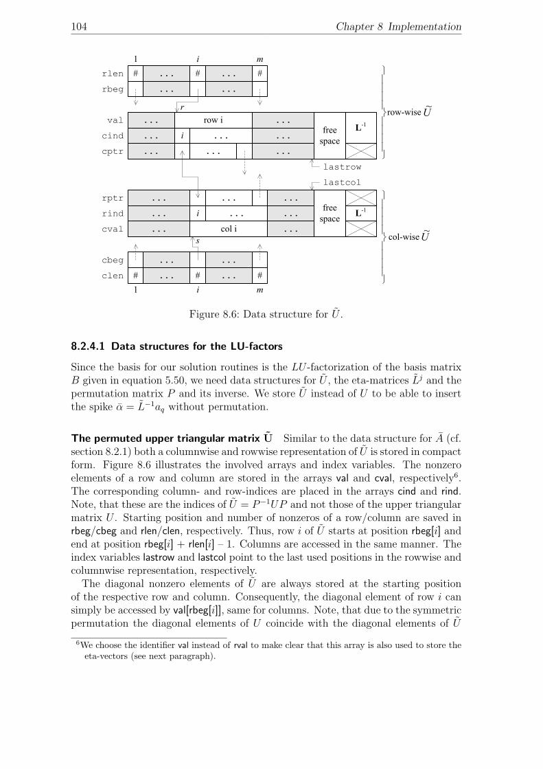
104 Chapter 8 Implementation
4444 84444 764444 84444 76
rlen
rbeg
mi1
row i
i ...
val
cind
cptr
...
...
... ...
...
...
...
col i
i ...
rptr
rind
cval
...
...
...
... ...
...
...
#
cbeg
clen
mi1
...
...
...
...
...
...
...
...# #
# # #
free space
free space
L-1
L-1
val...
lbeg
...
1...
netaf 2
......
...
......
neta
free space
etas from LUF
rind.........*...*
cind*............
U
*
⎪⎪⎪⎪
⎭
⎪⎪⎪⎪
⎬
⎫
⎪⎪⎪⎪
⎭
⎪⎪⎪⎪
⎬
⎫
row-wise
col-wise
etas from LUU
1 netaf
...etacol
1 mcoleta
j
lenlulbeg(neta+1)+1 lbeg(netaf+1) lbeg(netaf+1)+1
1
4
3
6
5
2
lastrow
lastcol
p
...
......
r
s
lbeg(1)
lstart
U~
U~
Figure 8.6: Data structure for U .
8.2.4.1 Data structures for the LU-factors
Since the basis for our solution routines is the LU -factorization of the basis matrixB given in equation 5.50, we need data structures for U , the eta-matrices Lj and thepermutation matrix P and its inverse. We store U instead of U to be able to insertthe spike α = L−1aq without permutation.
The permuted upper triangular matrix U Similar to the data structure for A (cf.section 8.2.1) both a columnwise and rowwise representation of U is stored in compactform. Figure 8.6 illustrates the involved arrays and index variables. The nonzeroelements of a row and column are stored in the arrays val and cval, respectively6.The corresponding column- and row-indices are placed in the arrays cind and rind.Note, that these are the indices of U = P−1UP and not those of the upper triangularmatrix U . Starting position and number of nonzeros of a row/column are saved inrbeg/cbeg and rlen/clen, respectively. Thus, row i of U starts at position rbeg[i] andend at position rbeg[i] + rlen[i] – 1. Columns are accessed in the same manner. Theindex variables lastrow and lastcol point to the last used positions in the rowwise andcolumnwise representation, respectively.
The diagonal nonzero elements of U are always stored at the starting positionof the respective row and column. Consequently, the diagonal element of row i cansimply be accessed by val[rbeg[i]], same for columns. Note, that due to the symmetricpermutation the diagonal elements of U coincide with the diagonal elements of U
6We choose the identifier val instead of rval to make clear that this array is also used to store theeta-vectors (see next paragraph).
8.2 The dual simplex code 105
4444 84444 764444 84444 76
rlen
rbeg
mi1
row i
i ...
val
cind
cptr
...
...
... ...
...
...
...
col i
i ...
rptr
rind
cval
...
...
...
... ...
...
...
#
cbeg
clen
mi1
...
...
...
...
...
...
...
...# #
# # #
free space
free space
L-1
L-1
val...
lbeg
...
1...
netaf 2
......
...
......
neta
free space
etas from LUF
rind.........*...*
cind*............
U
*
⎪⎪⎪⎪
⎭
⎪⎪⎪⎪
⎬
⎫
⎪⎪⎪⎪
⎭
⎪⎪⎪⎪
⎬
⎫
row-wise
col-wise
etas from LUU
1 netaf
...etacol
1 mcoleta
j
lenlulbeg(neta+1)+1 lbeg(netaf+1) lbeg(netaf+1)+1
1
4
3
6
5
2
lastrow
lastcol
p
...
......
r
s
lbeg(1)
lstart
U~
U~
Figure 8.7: Data structure for the eta vectors of L−1 (1).
(with changed positions). The order of the remaining elements is arbitrary.Unlike the problem matrix A the matrix U has to be updated in every iteration
in the LU -update procedure. To allow for an efficient update of its column- androwwise representation we deploy two further arrays cptr and rptr. For every nonzeroelement of the rowwise representation cptr contains the corresponding index in thecolumnwise representation, vice versa for rptr. Given these arrays it would actuallysuffice to store the nonzeros of U only once – say rowwise – columnwise access wouldstill be possible. However, this would result in a suboptimal usage of the processor’scache memory (cf. [68]). Therefore we keep holding two copies of the numericalvalues.
Columns corresponding to logical variables are always permuted to the beginningof U . They are not stored explicitly, only their number is kept in the variable nlogic.
The eta-vectors of L−1 For the eta-matrices Lj we partly use the same arrays asfor U . Only the nonzero elements of the nontrivial column/row of an eta-matrix arestored in the array val starting from its tail (see figure 8.7). The starting positionof each eta-vector is noted in the array lbeg. The first netaf entries correspondto column-eta-vectors from the LU -factorization, followed by the row-eta-vectorsgenerated in LU -update. The total number of eta-vectors is neta. The arrays rindand cind contain the associated row and column indices. Consequently, the areas infigure 8.7, which are marked with a *, contain the same entry for all elements of aneta-vector. In the variables lstart and lenlu we keep the first and the last position ofan element of L−1. nentl corresponds to the total number of nonzero elements of alleta-vectors.
For each eta-matrix Lj (1 ≤ j ≤ netaf) from LU -factorization we also store theindex of the nontrivial column in etacol[j]. The array coleta constitutes the inverseof etacol (see figure 8.8). If for a column p no eta vector exists, we set coleta[p] = 0.
The permutation As mentioned before we store U = P TUP and not U . To be ableto reconstruct U (e.g. in FTranU and BTranU) the permutation has to be stored andupdated explicitly. Since the rows and columns of U are permuted symmetrically,
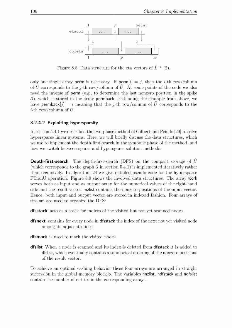
106 Chapter 8 Implementation
4444 84444 764444 84444 76
rlen
rbeg
mi1
row i
i ...
val
cind
cptr
...
...
... ...
...
...
...
col i
i ...
rptr
rind
cval
...
...
...
... ...
...
...
#
cbeg
clen
mi1
...
...
...
...
...
...
...
...# #
# # #
free space
free space
L-1
L-1
val...
lbeg
...
1...
netaf 2
......
...
......
neta
free space
etas from LUF
rind.........*...*
cind*............
U
*
⎪⎪⎪⎪
⎭
⎪⎪⎪⎪
⎬
⎫
⎪⎪⎪⎪
⎭
⎪⎪⎪⎪
⎬
⎫
row-wise
col-wise
etas from LUU
1 netaf
...etacol
1 mcoleta
j
lenlulbeg(neta+1)+1 lbeg(netaf+1) lbeg(netaf+1)+1
1
4
3
6
5
2
lastrow
lastcol
p
...
......
r
s
lbeg(1)
lstart
U~
U~
Figure 8.8: Data structure for the eta vectors of L−1 (2).
only one single array perm is necessary. If perm[i] = j, then the i-th row/columnof U corresponds to the j-th row/column of U . At some points of the code we alsoneed the inverse of perm (e.g., to determine the last nonzero position in the spikeα), which is stored in the array permback. Extending the example from above, wehave permback[j] = i meaning that the j-th row/column of U corresponds to thei-th row/column of U .
8.2.4.2 Exploiting hypersparsity
In section 5.4.1 we described the two-phase method of Gilbert and Peierls [29] to solvehypersparse linear systems. Here, we will briefly discuss the data structures, whichwe use to implement the depth-first-search in the symbolic phase of the method, andhow we switch between sparse and hypersparse solution methods.
Depth-first-search The depth-first-search (DFS) on the compact storage of U(which corresponds to the graph G in section 5.4.1) is implemented iteratively ratherthan recursively. In algorithm 24 we give detailed pseudo code for the hypersparseFTranU operation. Figure 8.9 shows the involved data structures. The array workserves both as input and as output array for the numerical values of the right-handside and the result vector. nzlist contains the nonzero positions of the input vector.Hence, both input and output vector are stored in indexed fashion. Four arrays ofsize xm are used to organize the DFS:
dfsstack acts as a stack for indices of the visited but not yet scanned nodes.
dfsnext contains for every node in dfsstack the index of the next not yet visited nodeamong its adjacent nodes.
dfsmark is used to mark the visited nodes.
dfslist When a node is scanned and its index is deleted from dfsstack it is added todfslist, which eventually contains a topological ordering of the nonzero positionsof the result vector.
To achieve an optimal cashing behavior these four arrays are arranged in straightsuccession in the global memory block b. The variables nnzlist, ndfstack and ndfslistcontain the number of entries in the corresponding arrays.
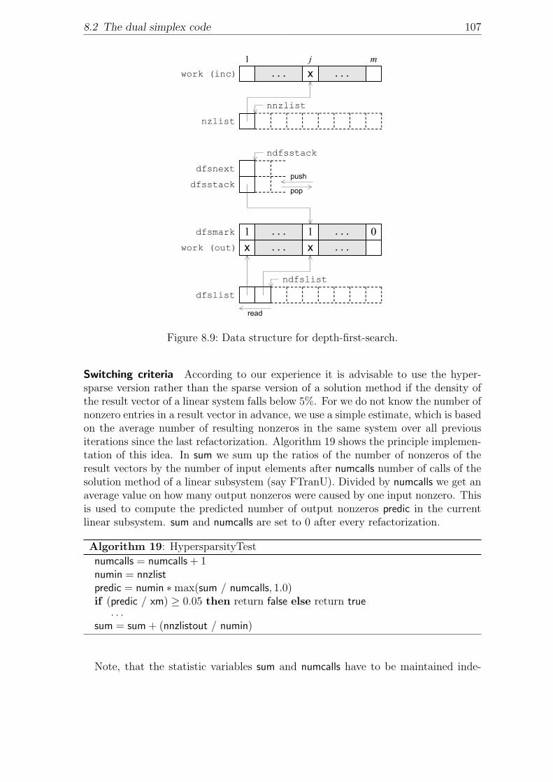
8.2 The dual simplex code 107
... ...1 01
mj1... ...x
nzlist
work (inc)
dfslist
... ...x x
read
work (out)
push
popdfsstack
dfsnext
dfsmark
nnzlist
ndfsstack
ndfslist
1 m... ...x ...x... ...0 ... 01 1
nzlist
nnzlist
mark
work
FTRANL
1 m... ...x ...x... ...0 ...1 1
nnzlist
mark
spike x1
nzlist
FTRANU
1 m... ...x ...
nnzlistout
work x
nzlistout
xx
Figure 8.9: Data structure for depth-first-search.
Switching criteria According to our experience it is advisable to use the hyper-sparse version rather than the sparse version of a solution method if the density ofthe result vector of a linear system falls below 5%. For we do not know the number ofnonzero entries in a result vector in advance, we use a simple estimate, which is basedon the average number of resulting nonzeros in the same system over all previousiterations since the last refactorization. Algorithm 19 shows the principle implemen-tation of this idea. In sum we sum up the ratios of the number of nonzeros of theresult vectors by the number of input elements after numcalls number of calls of thesolution method of a linear subsystem (say FTranU). Divided by numcalls we get anaverage value on how many output nonzeros were caused by one input nonzero. Thisis used to compute the predicted number of output nonzeros predic in the currentlinear subsystem. sum and numcalls are set to 0 after every refactorization.
Algorithm 19: HypersparsityTest
numcalls = numcalls + 1numin = nnzlistpredic = numin ∗max(sum / numcalls, 1.0)if (predic / xm) ≥ 0.05 then return false else return true
. . .sum = sum + (nnzlistout / numin)
Note, that the statistic variables sum and numcalls have to be maintained inde-
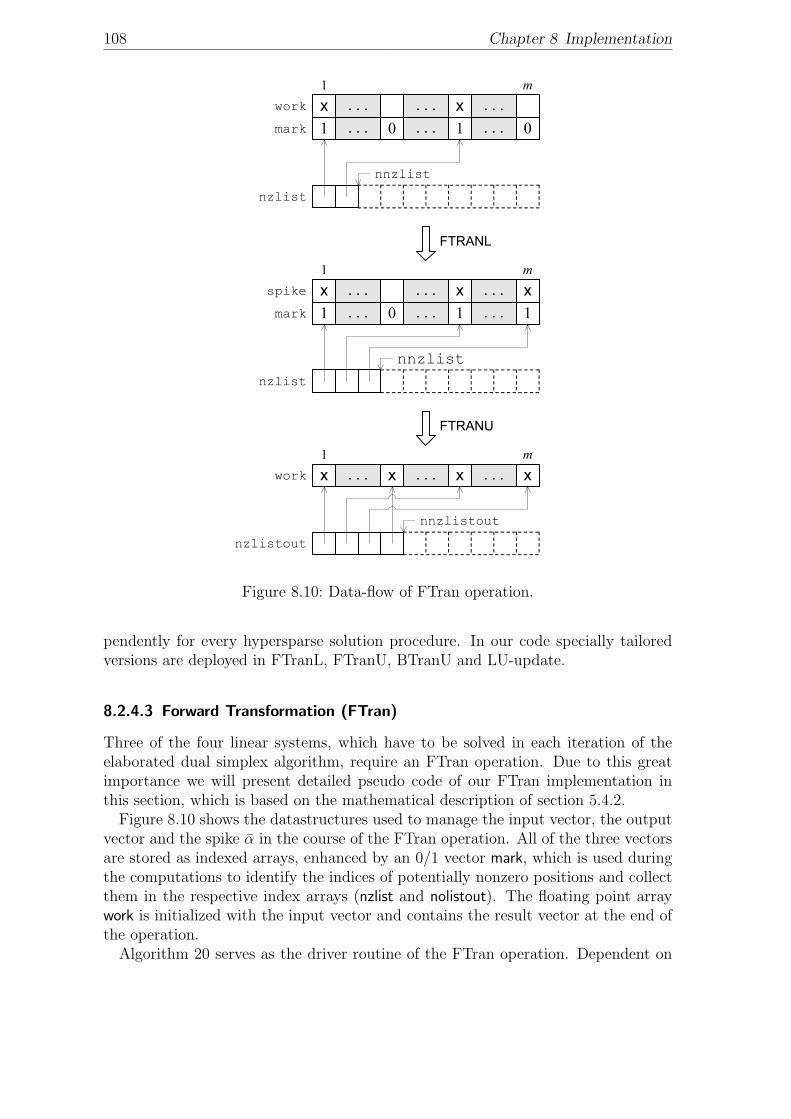
108 Chapter 8 Implementation
... ...1 01
mj1... ...x
nzlist
work (inc)
dfslist
... ...x x
read
work (out)
push
popdfsstack
dfsnext
dfsmark
nnzlist
ndfsstack
ndfslist
1 m... ...x ...x... ...0 ... 01 1
nzlist
nnzlist
mark
work
FTRANL
1 m... ...x ...x... ...0 ...1 1
nnzlist
mark
spike x1
nzlist
FTRANU
1 m... ...x ...
nnzlistout
work x
nzlistout
xx
Figure 8.10: Data-flow of FTran operation.
pendently for every hypersparse solution procedure. In our code specially tailoredversions are deployed in FTranL, FTranU, BTranU and LU-update.
8.2.4.3 Forward Transformation (FTran)
Three of the four linear systems, which have to be solved in each iteration of theelaborated dual simplex algorithm, require an FTran operation. Due to this greatimportance we will present detailed pseudo code of our FTran implementation inthis section, which is based on the mathematical description of section 5.4.2.
Figure 8.10 shows the datastructures used to manage the input vector, the outputvector and the spike α in the course of the FTran operation. All of the three vectorsare stored as indexed arrays, enhanced by an 0/1 vector mark, which is used duringthe computations to identify the indices of potentially nonzero positions and collectthem in the respective index arrays (nzlist and nolistout). The floating point arraywork is initialized with the input vector and contains the result vector at the end ofthe operation.
Algorithm 20 serves as the driver routine of the FTran operation. Dependent on
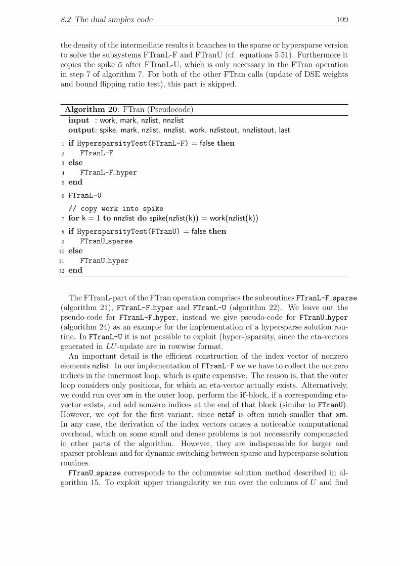
8.2 The dual simplex code 109
the density of the intermediate results it branches to the sparse or hypersparse versionto solve the subsystems FTranL-F and FTranU (cf. equations 5.51). Furthermore itcopies the spike α after FTranL-U, which is only necessary in the FTran operationin step 7 of algorithm 7. For both of the other FTran calls (update of DSE weightsand bound flipping ratio test), this part is skipped.
Algorithm 20: FTran (Pseudocode)
input : work, mark, nzlist, nnzlistoutput: spike, mark, nzlist, nnzlist, work, nzlistout, nnzlistout, last
if HypersparsityTest(FTranL-F) = false then1
FTranL-F2
else3
FTranL-F hyper4
end5
FTranL-U6
// copy work into spike
for k = 1 to nnzlist do spike(nzlist(k)) = work(nzlist(k))7
if HypersparsityTest(FTranU) = false then8
FTranU sparse9
else10
FTranU hyper11
end12
The FTranL-part of the FTran operation comprises the subroutines FTranL-F sparse
(algorithm 21), FTranL-F hyper and FTranL-U (algorithm 22). We leave out thepseudo-code for FTranL-F hyper, instead we give pseudo-code for FTranU hyper
(algorithm 24) as an example for the implementation of a hypersparse solution rou-tine. In FTranL-U it is not possible to exploit (hyper-)sparsity, since the eta-vectorsgenerated in LU -update are in rowwise format.
An important detail is the efficient construction of the index vector of nonzeroelements nzlist. In our implementation of FTranL-F we we have to collect the nonzeroindices in the innermost loop, which is quite expensive. The reason is, that the outerloop considers only positions, for which an eta-vector actually exists. Alternatively,we could run over xm in the outer loop, perform the if -block, if a corresponding eta-vector exists, and add nonzero indices at the end of that block (similar to FTranU).However, we opt for the first variant, since netaf is often much smaller that xm.In any case, the derivation of the index vectors causes a noticeable computationaloverhead, which on some small and dense problems is not necessarily compensatedin other parts of the algorithm. However, they are indispensable for larger andsparser problems and for dynamic switching between sparse and hypersparse solutionroutines.FTranU sparse corresponds to the columnwise solution method described in al-
gorithm 15. To exploit upper triangularity we run over the columns of U and find
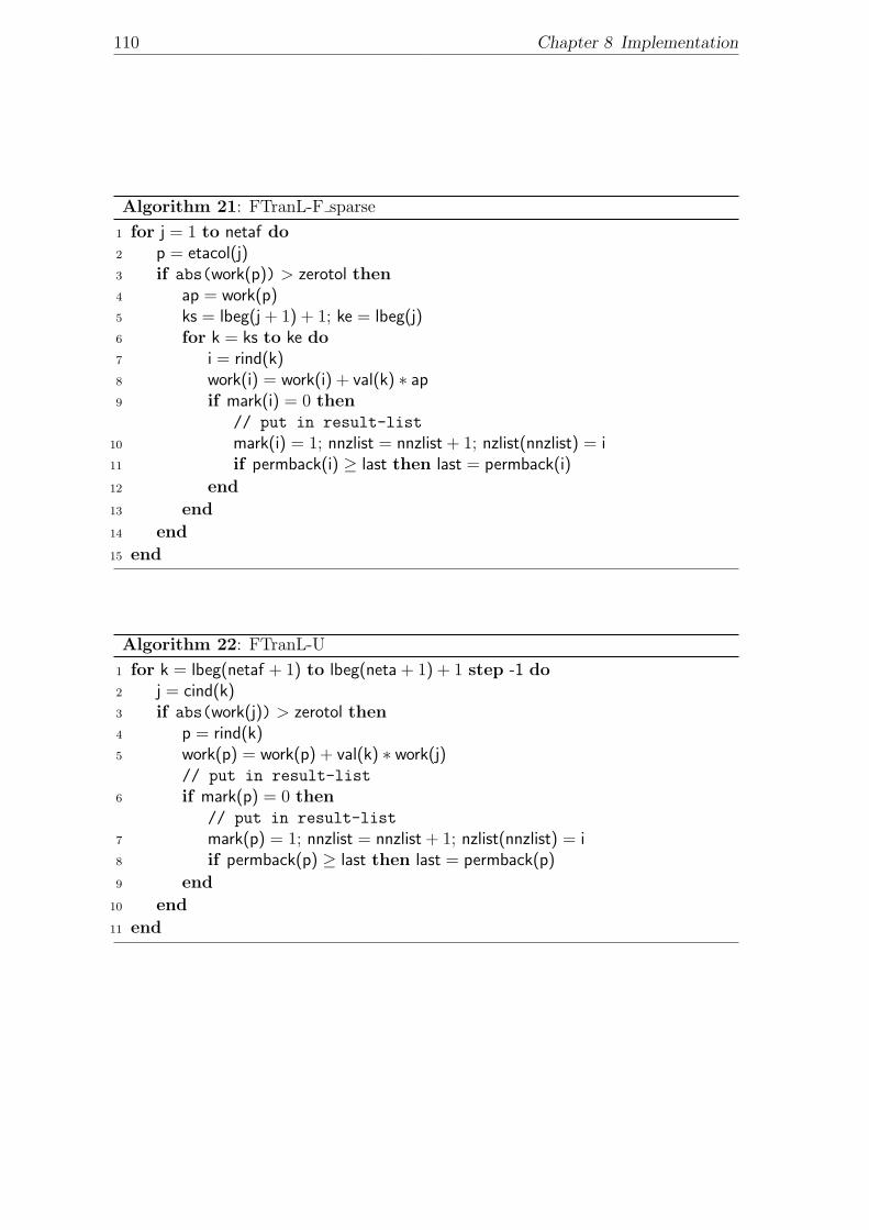
110 Chapter 8 Implementation
Algorithm 21: FTranL-F sparse
for j = 1 to netaf do1
p = etacol(j)2
if abs(work(p)) > zerotol then3
ap = work(p)4
ks = lbeg(j + 1) + 1; ke = lbeg(j)5
for k = ks to ke do6
i = rind(k)7
work(i) = work(i) + val(k) ∗ ap8
if mark(i) = 0 then9
// put in result-list
mark(i) = 1; nnzlist = nnzlist + 1; nzlist(nnzlist) = i10
if permback(i) ≥ last then last = permback(i)11
end12
end13
end14
end15
Algorithm 22: FTranL-U
for k = lbeg(netaf + 1) to lbeg(neta + 1) + 1 step -1 do1
j = cind(k)2
if abs(work(j)) > zerotol then3
p = rind(k)4
work(p) = work(p) + val(k) ∗ work(j)5
// put in result-list
if mark(p) = 0 then6
// put in result-list
mark(p) = 1; nnzlist = nnzlist + 1; nzlist(nnzlist) = i7
if permback(p) ≥ last then last = permback(p)8
end9
end10
end11
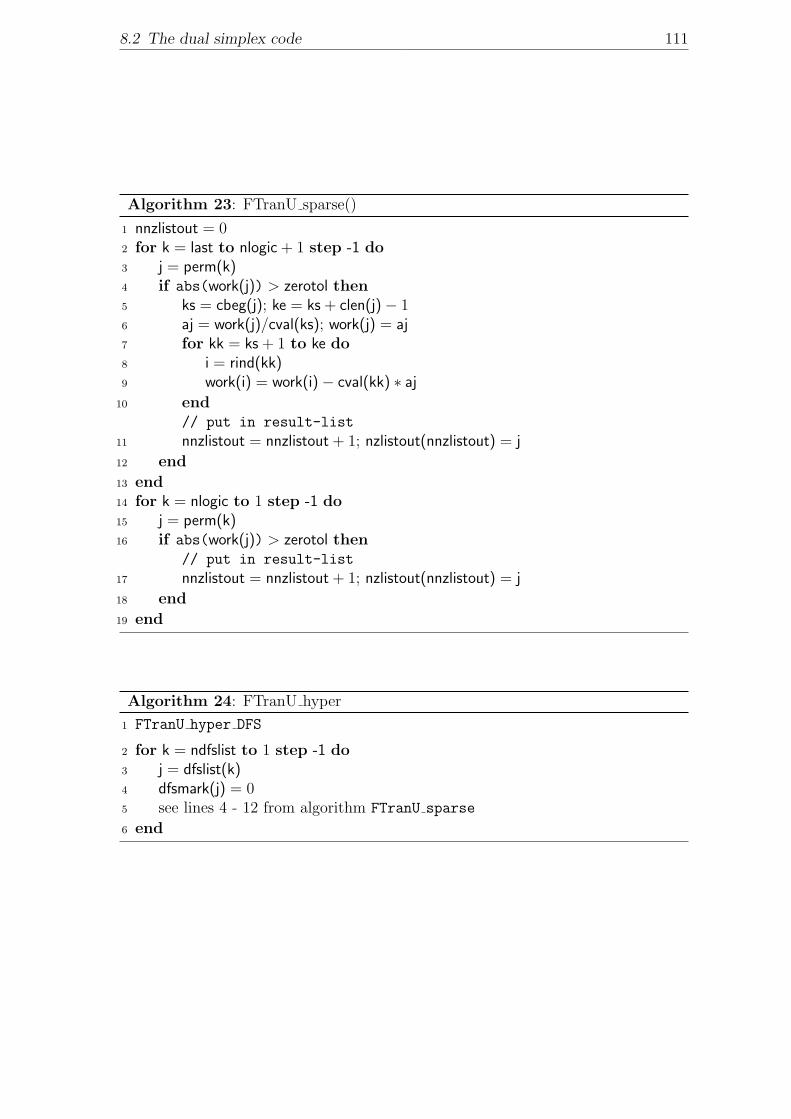
8.2 The dual simplex code 111
Algorithm 23: FTranU sparse()
nnzlistout = 01
for k = last to nlogic + 1 step -1 do2
j = perm(k)3
if abs(work(j)) > zerotol then4
ks = cbeg(j); ke = ks + clen(j)− 15
aj = work(j)/cval(ks); work(j) = aj6
for kk = ks + 1 to ke do7
i = rind(kk)8
work(i) = work(i)− cval(kk) ∗ aj9
end10
// put in result-list
nnzlistout = nnzlistout + 1; nzlistout(nnzlistout) = j11
end12
end13
for k = nlogic to 1 step -1 do14
j = perm(k)15
if abs(work(j)) > zerotol then16
// put in result-list
nnzlistout = nnzlistout + 1; nzlistout(nnzlistout) = j17
end18
end19
Algorithm 24: FTranU hyper
FTranU hyper DFS1
for k = ndfslist to 1 step -1 do2
j = dfslist(k)3
dfsmark(j) = 04
see lines 4 - 12 from algorithm FTranU sparse5
end6
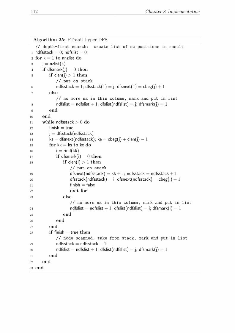
112 Chapter 8 Implementation
Algorithm 25: FTranU hyper DFS
// depth-first search: create list of nz positions in result
ndfsstack = 0; ndfslist = 01
for k = 1 to nnzlist do2
j = nzlist(k)3
if dfsmark(j) = 0 then4
if clen(j) > 1 then5
// put on stack
ndfsstack = 1; dfsstack(1) = j; dfsnext(1) = cbeg(j) + 16
else7
// no more nz in this column, mark and put in list
ndfslist = ndfslist + 1; dfslist(ndfslist) = j; dfsmark(j) = 18
end9
end10
while ndfsstack > 0 do11
finish = true12
j = dfsstack(ndfsstack)13
ks = dfsnext(ndfsstack); ke = cbeg(j) + clen(j)− 114
for kk = ks to ke do15
i = rind(kk)16
if dfsmark(i) = 0 then17
if clen(i) > 1 then18
// put on stack
dfsnext(ndfsstack) = kk + 1; ndfsstack = ndfsstack + 119
dfsstack(ndfsstack) = i; dfsnext(ndfsstack) = cbeg(i) + 120
finish = false21
exit for22
else23
// no more nz in this column, mark and put in list
ndfslist = ndfslist + 1; dfslist(ndfslist) = i; dfsmark(i) = 124
end25
end26
end27
if finish = true then28
// node scanned, take from stack, mark and put in list
ndfsstack = ndfsstack− 129
ndfslist = ndfslist + 1; dfslist(ndfslist) = j; dfsmark(j) = 130
end31
end32
end33
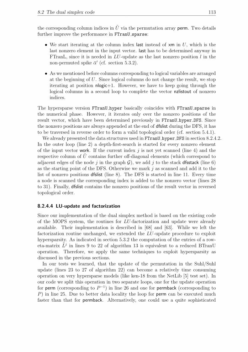
8.2 The dual simplex code 113
the corresponding column indices in U via the permutation array perm. Two detailsfurther improve the performance in FTranU sparse:
• We start iterating at the column index last instead of xm in U , which is thelast nonzero element in the input vector. last has to be determined anyway inFTranL, since it is needed in LU -update as the last nonzero position l in thenon-permuted spike α′ (cf. section 5.3.2).
• As we mentioned before columns corresponding to logical variables are arrangedat the beginning of U . Since logical columns do not change the result, we stopiterating at position nlogic+1. However, we have to keep going through thelogical columns in a second loop to complete the vector nzlistout of nonzeroindices.
The hypersparse version FTranU hyper basically coincides with FTranU sparse inthe numerical phase. However, it iterates only over the nonzero positions of theresult vector, which have been determined previously in FTranU hyper DFS. Sincethe nonzero positions are always appended at the end of dfslist during the DFS, it hasto be traversed in reverse order to form a valid topological order (cf. section 5.4.1).
We already presented the data structures used in FTranU hyper DFS in section 8.2.4.2.In the outer loop (line 2) a depth-first-search is started for every nonzero elementof the input vector work. If the current index j is not yet scanned (line 4) and therespective column of U contains further off-diagonal elements (which correspond toadjacent edges of the node j in the graph G), we add j to the stack dfsstack (line 6)as the starting point of the DFS. Otherwise we mark j as scanned and add it to thelist of nonzero positions dfslist (line 8). The DFS is started in line 11. Every timea node is scanned the corresponding index is added to the nonzero vector (lines 28to 31). Finally, dfslist contains the nonzero positions of the result vector in reversedtopological order.
8.2.4.4 LU-update and factorization
Since our implementation of the dual simplex method is based on the existing codeof the MOPS system, the routines for LU -factorization and update were alreadyavailable. Their implementation is described in [68] and [63]. While we left thefactorization routine unchanged, we extended the LU -update procedure to exploithypersparsity. As indicated in section 5.3.2 the computation of the entries of a row-eta-matrix Lj in lines 9 to 22 of algorithm 13 is equivalent to a reduced BTranUoperation. Therefore, we apply the same techniques to exploit hypersparsity asdiscussed in the previous sections.
In our tests we learned, that the update of the permutation in the Suhl/Suhlupdate (lines 23 to 27 of algorithm 22) can become a relatively time consumingoperation on very hypersparse models (like ken-18 from the NetLib [5] test set). Inour code we split this operation in two separate loops, one for the update operationfor perm (corresponding to P−1) in line 26 and one for permback (corresponding toP ) in line 25. Due to better data locality the loop for perm can be executed muchfaster than that for permback. Alternatively, one could use a quite sophisticated
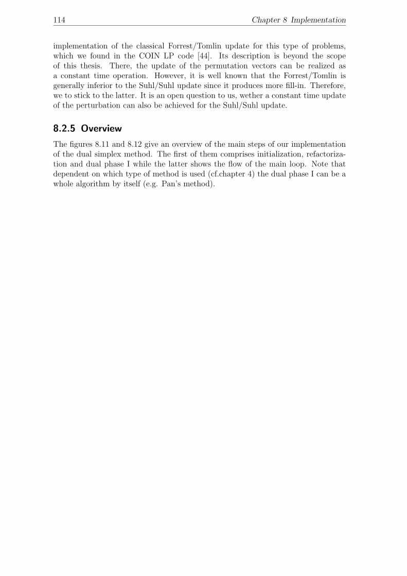
114 Chapter 8 Implementation
implementation of the classical Forrest/Tomlin update for this type of problems,which we found in the COIN LP code [44]. Its description is beyond the scopeof this thesis. There, the update of the permutation vectors can be realized asa constant time operation. However, it is well known that the Forrest/Tomlin isgenerally inferior to the Suhl/Suhl update since it produces more fill-in. Therefore,we to stick to the latter. It is an open question to us, wether a constant time updateof the perturbation can also be achieved for the Suhl/Suhl update.
8.2.5 Overview
The figures 8.11 and 8.12 give an overview of the main steps of our implementationof the dual simplex method. The first of them comprises initialization, refactoriza-tion and dual phase I while the latter shows the flow of the main loop. Note thatdependent on which type of method is used (cf.chapter 4) the dual phase I can be awhole algorithm by itself (e.g. Pan’s method).
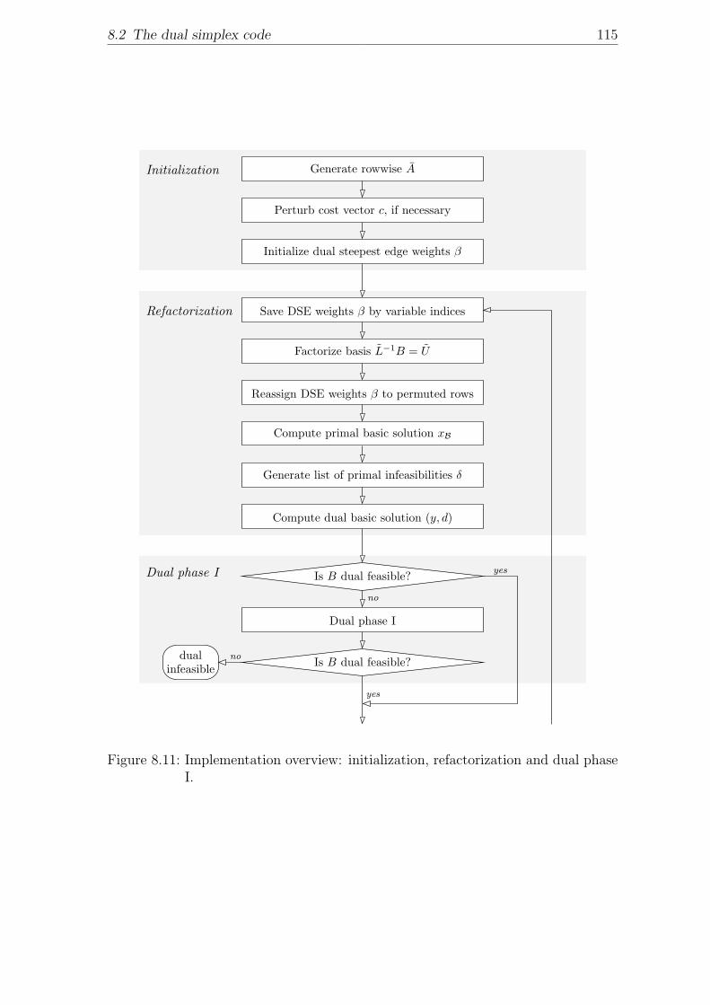
8.2 The dual simplex code 115
infeasibledual
Refactorization
yes
no
no
yes
Is B dual feasible?
Dual phase I
Is B dual feasible?
Initialize dual steepest edge weights β
Perturb cost vector c, if necessary
Generate rowwise A
Compute dual basic solution (y, d)
Reassign DSE weights β to permuted rows
Save DSE weights β by variable indices
Generate list of primal infeasibilities δ
Compute primal basic solution xB
Factorize basis L−1B = U
Initialization
Dual phase I
Figure 8.11: Implementation overview: initialization, refactorization and dual phaseI.
116 Chapter 8 Implementation
Unroll DSE weights
Update DSE weights β (save changed positions)
Update d, consider bound flips in xB and δ
no
no
(call primal simplex)
Remove perturbation
Remove perturbation
(call primal simplex)
unboundeddual
yes
no
no
yes
optimal
yes
yes
Need to factorize?
Consider bound flips in xN
Update xB and δ
Error in LU-Update?
LU-Update
Compute pivot column: Bαq = aq
FTran αrq ≈ BTran αr
q
Compute pivot row: BT ρr = er, αr = ρTr AN
Found q?
BF ratio test: find entering variable q
Found p?
Main loop Pricing: find primal inf. leaving variable p
yes
no
Figure 8.12: Implementation overview: main loop.
117
Chapter 9
Numerical results
In this chapter we present computational results produced by our dual simplex code.In sections 9.1 and 9.2 we describe the composition of our set of test problems andthe performance measures used in our analysis. We then present a study on thedual phase 1 in section 9.3, where we evaluate the performance of the different dualphase 1 methods described in chapter 4. In section 9.4 we document the continuousprogress during the development of our code and point out again the crucial imple-mentation techniques. Finally, we benchmark the performance of our dual simplexcode compared to other renowned LP-systems in section 9.5.
9.1 Test problems
Table A.1 specifies names and dimensions of a set of one hundred test problems,which constitute the basis for the computational results of this chapter. The prob-lems are taken from five different sources (column Source):
n NetLib and Kennington test set [5], 17 problems.
m MipLib2003 test set [3], 17 problems1.
t Mittelmann test set [4], 21 problems.
c BPMPD test set [1], 20 problems.
o Other. 25 problems from our private test problem collection [2]. The prob-lems HAL M D, MUN1 M D, MUN18 M D and PTV15 are multi-depot busscheduling models described in [37].
In addition, we generated a second, preprocessed version of each problem instanceby means of the COIN LP code2[44]. These pretreated instances will be used insection 9.5 to benchmark the dual simplex implementations of the different LP-systems independently of their respective LP-preprocessing. For both versions wegive the model dimensions in terms of the number of structural variables (columnStructs), the number of constraints (column Constrs) and the number of nonzeroentries in the constraint matrix (column Nzs).
1We only solve the LP-relaxation of these problems.2At the beginning of the method ClpSimplexDual::dual(. . . ) we write out the preprocessed model
in MPS format (see [50] for a description) using the method writeMps(. . . ).
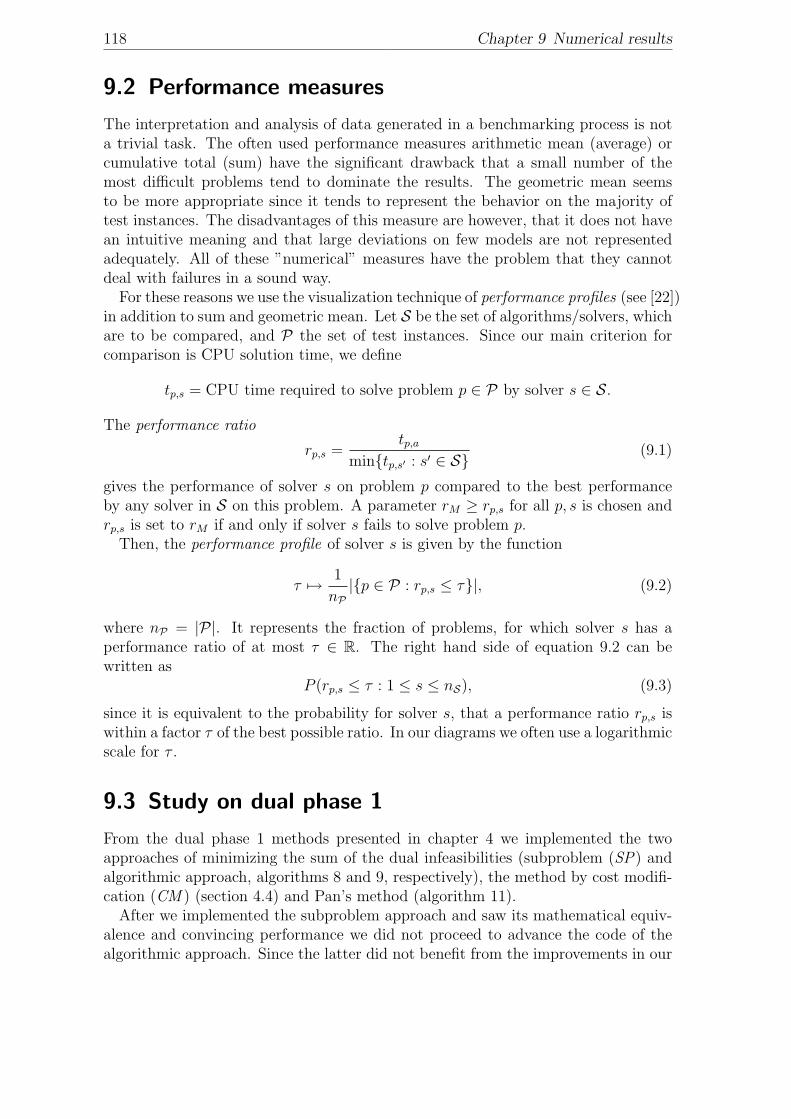
118 Chapter 9 Numerical results
9.2 Performance measures
The interpretation and analysis of data generated in a benchmarking process is nota trivial task. The often used performance measures arithmetic mean (average) orcumulative total (sum) have the significant drawback that a small number of themost difficult problems tend to dominate the results. The geometric mean seemsto be more appropriate since it tends to represent the behavior on the majority oftest instances. The disadvantages of this measure are however, that it does not havean intuitive meaning and that large deviations on few models are not representedadequately. All of these ”numerical” measures have the problem that they cannotdeal with failures in a sound way.
For these reasons we use the visualization technique of performance profiles (see [22])in addition to sum and geometric mean. Let S be the set of algorithms/solvers, whichare to be compared, and P the set of test instances. Since our main criterion forcomparison is CPU solution time, we define
tp,s = CPU time required to solve problem p ∈ P by solver s ∈ S.
The performance ratio
rp,s =tp,a
min{tp,s′ : s′ ∈ S}(9.1)
gives the performance of solver s on problem p compared to the best performanceby any solver in S on this problem. A parameter rM ≥ rp,s for all p, s is chosen andrp,s is set to rM if and only if solver s fails to solve problem p.
Then, the performance profile of solver s is given by the function
τ 7→ 1
nP|{p ∈ P : rp,s ≤ τ}|, (9.2)
where nP = |P|. It represents the fraction of problems, for which solver s has aperformance ratio of at most τ ∈ R. The right hand side of equation 9.2 can bewritten as
P (rp,s ≤ τ : 1 ≤ s ≤ nS), (9.3)
since it is equivalent to the probability for solver s, that a performance ratio rp,s iswithin a factor τ of the best possible ratio. In our diagrams we often use a logarithmicscale for τ .
9.3 Study on dual phase 1
From the dual phase 1 methods presented in chapter 4 we implemented the twoapproaches of minimizing the sum of the dual infeasibilities (subproblem (SP) andalgorithmic approach, algorithms 8 and 9, respectively), the method by cost modifi-cation (CM ) (section 4.4) and Pan’s method (algorithm 11).
After we implemented the subproblem approach and saw its mathematical equiv-alence and convincing performance we did not proceed to advance the code of thealgorithmic approach. Since the latter did not benefit from the improvements in our
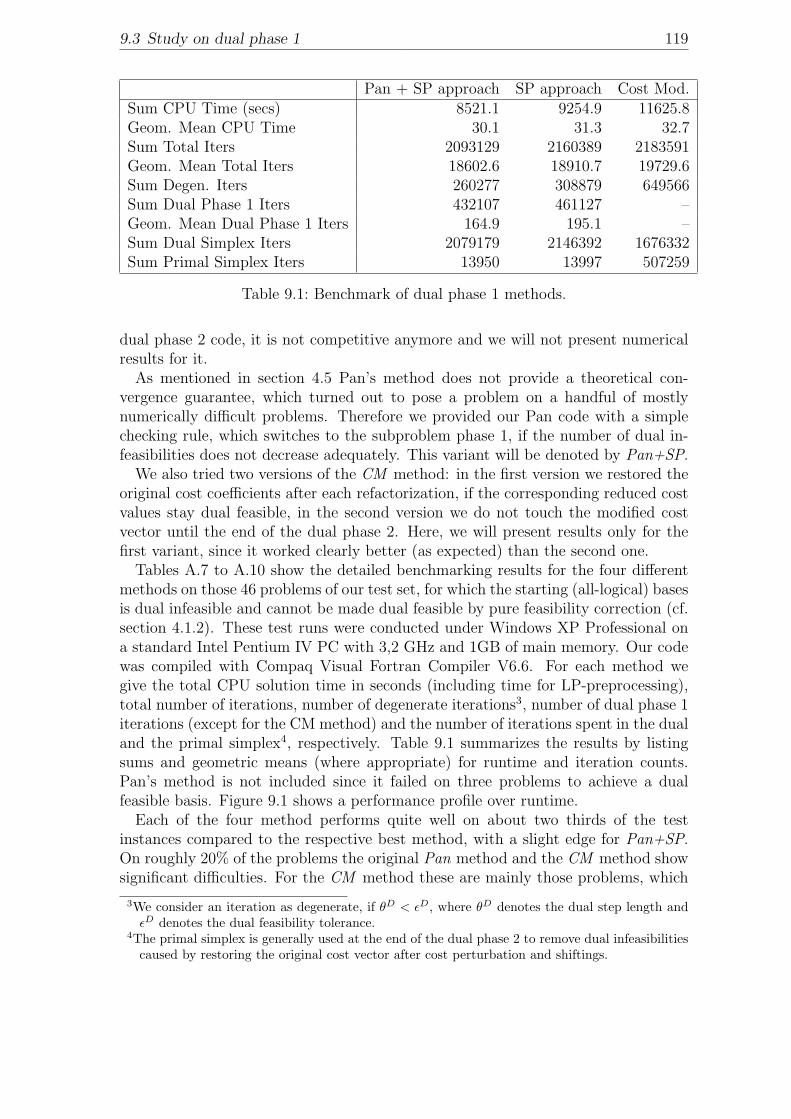
9.3 Study on dual phase 1 119
Pan + SP approach SP approach Cost Mod.Sum CPU Time (secs) 8521.1 9254.9 11625.8Geom. Mean CPU Time 30.1 31.3 32.7Sum Total Iters 2093129 2160389 2183591Geom. Mean Total Iters 18602.6 18910.7 19729.6Sum Degen. Iters 260277 308879 649566Sum Dual Phase 1 Iters 432107 461127 –Geom. Mean Dual Phase 1 Iters 164.9 195.1 –Sum Dual Simplex Iters 2079179 2146392 1676332Sum Primal Simplex Iters 13950 13997 507259
Table 9.1: Benchmark of dual phase 1 methods.
dual phase 2 code, it is not competitive anymore and we will not present numericalresults for it.
As mentioned in section 4.5 Pan’s method does not provide a theoretical con-vergence guarantee, which turned out to pose a problem on a handful of mostlynumerically difficult problems. Therefore we provided our Pan code with a simplechecking rule, which switches to the subproblem phase 1, if the number of dual in-feasibilities does not decrease adequately. This variant will be denoted by Pan+SP.
We also tried two versions of the CM method: in the first version we restored theoriginal cost coefficients after each refactorization, if the corresponding reduced costvalues stay dual feasible, in the second version we do not touch the modified costvector until the end of the dual phase 2. Here, we will present results only for thefirst variant, since it worked clearly better (as expected) than the second one.
Tables A.7 to A.10 show the detailed benchmarking results for the four differentmethods on those 46 problems of our test set, for which the starting (all-logical) basesis dual infeasible and cannot be made dual feasible by pure feasibility correction (cf.section 4.1.2). These test runs were conducted under Windows XP Professional ona standard Intel Pentium IV PC with 3,2 GHz and 1GB of main memory. Our codewas compiled with Compaq Visual Fortran Compiler V6.6. For each method wegive the total CPU solution time in seconds (including time for LP-preprocessing),total number of iterations, number of degenerate iterations3, number of dual phase 1iterations (except for the CM method) and the number of iterations spent in the dualand the primal simplex4, respectively. Table 9.1 summarizes the results by listingsums and geometric means (where appropriate) for runtime and iteration counts.Pan’s method is not included since it failed on three problems to achieve a dualfeasible basis. Figure 9.1 shows a performance profile over runtime.
Each of the four method performs quite well on about two thirds of the testinstances compared to the respective best method, with a slight edge for Pan+SP.On roughly 20% of the problems the original Pan method and the CM method showsignificant difficulties. For the CM method these are mainly those problems, which
3We consider an iteration as degenerate, if θD < εD, where θD denotes the dual step length andεD denotes the dual feasibility tolerance.
4The primal simplex is generally used at the end of the dual phase 2 to remove dual infeasibilitiescaused by restoring the original cost vector after cost perturbation and shiftings.
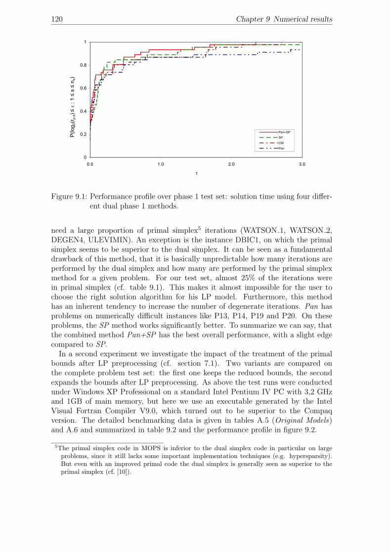
120 Chapter 9 Numerical results
0
0.2
0.4
0.6
0.8
1
0.0 1.0 2.0 3.0
Pan+SP
SP
CM
Pan
τ
P(lo
g 2(r p
,s) ≤
τ :
1 ≤
s ≤
n s)
Figure 9.1: Performance profile over phase 1 test set: solution time using four differ-ent dual phase 1 methods.
need a large proportion of primal simplex5 iterations (WATSON 1, WATSON 2,DEGEN4, ULEVIMIN). An exception is the instance DBIC1, on which the primalsimplex seems to be superior to the dual simplex. It can be seen as a fundamentaldrawback of this method, that it is basically unpredictable how many iterations areperformed by the dual simplex and how many are performed by the primal simplexmethod for a given problem. For our test set, almost 25% of the iterations werein primal simplex (cf. table 9.1). This makes it almost impossible for the user tochoose the right solution algorithm for his LP model. Furthermore, this methodhas an inherent tendency to increase the number of degenerate iterations. Pan hasproblems on numerically difficult instances like P13, P14, P19 and P20. On theseproblems, the SP method works significantly better. To summarize we can say, thatthe combined method Pan+SP has the best overall performance, with a slight edgecompared to SP.
In a second experiment we investigate the impact of the treatment of the primalbounds after LP preprocessing (cf. section 7.1). Two variants are compared onthe complete problem test set: the first one keeps the reduced bounds, the secondexpands the bounds after LP preprocessing. As above the test runs were conductedunder Windows XP Professional on a standard Intel Pentium IV PC with 3,2 GHzand 1GB of main memory, but here we use an executable generated by the IntelVisual Fortran Compiler V9.0, which turned out to be superior to the Compaqversion. The detailed benchmarking data is given in tables A.5 (Original Models)and A.6 and summarized in table 9.2 and the performance profile in figure 9.2.
5The primal simplex code in MOPS is inferior to the dual simplex code in particular on largeproblems, since it still lacks some important implementation techniques (e.g. hypersparsity).But even with an improved primal code the dual simplex is generally seen as superior to theprimal simplex (cf. [10]).
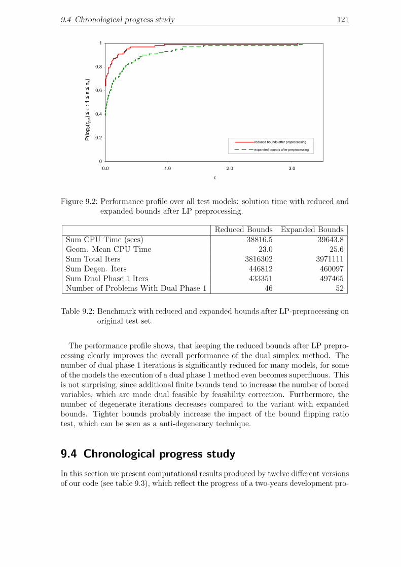
9.4 Chronological progress study 121
0
0.2
0.4
0.6
0.8
1
0.0 1.0 2.0 3.0
reduced bounds after preprocessing
expanded bounds after preprocessing
τ
P(lo
g 2(r p
,s) ≤
τ :
1 ≤
s ≤
n s)
Figure 9.2: Performance profile over all test models: solution time with reduced andexpanded bounds after LP preprocessing.
Reduced Bounds Expanded BoundsSum CPU Time (secs) 38816.5 39643.8Geom. Mean CPU Time 23.0 25.6Sum Total Iters 3816302 3971111Sum Degen. Iters 446812 460097Sum Dual Phase 1 Iters 433351 497465Number of Problems With Dual Phase 1 46 52
Table 9.2: Benchmark with reduced and expanded bounds after LP-preprocessing onoriginal test set.
The performance profile shows, that keeping the reduced bounds after LP prepro-cessing clearly improves the overall performance of the dual simplex method. Thenumber of dual phase 1 iterations is significantly reduced for many models, for someof the models the execution of a dual phase 1 method even becomes superfluous. Thisis not surprising, since additional finite bounds tend to increase the number of boxedvariables, which are made dual feasible by feasibility correction. Furthermore, thenumber of degenerate iterations decreases compared to the variant with expandedbounds. Tighter bounds probably increase the impact of the bound flipping ratiotest, which can be seen as a anti-degeneracy technique.
9.4 Chronological progress study
In this section we present computational results produced by twelve different versionsof our code (see table 9.3), which reflect the progress of a two-years development pro-
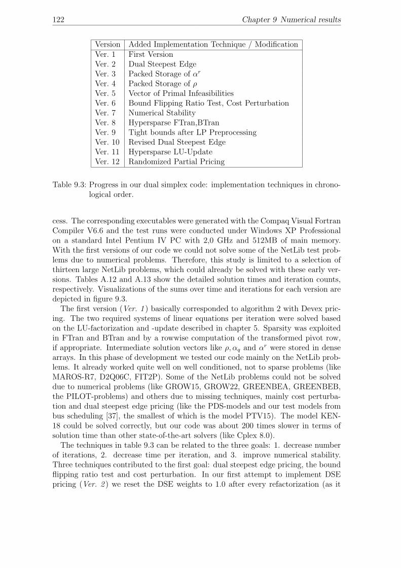
122 Chapter 9 Numerical results
Version Added Implementation Technique / ModificationVer. 1 First VersionVer. 2 Dual Steepest EdgeVer. 3 Packed Storage of αr
Ver. 4 Packed Storage of ρVer. 5 Vector of Primal InfeasibilitiesVer. 6 Bound Flipping Ratio Test, Cost PerturbationVer. 7 Numerical StabilityVer. 8 Hypersparse FTran,BTranVer. 9 Tight bounds after LP PreprocessingVer. 10 Revised Dual Steepest EdgeVer. 11 Hypersparse LU-UpdateVer. 12 Randomized Partial Pricing
Table 9.3: Progress in our dual simplex code: implementation techniques in chrono-logical order.
cess. The corresponding executables were generated with the Compaq Visual FortranCompiler V6.6 and the test runs were conducted under Windows XP Professionalon a standard Intel Pentium IV PC with 2,0 GHz and 512MB of main memory.With the first versions of our code we could not solve some of the NetLib test prob-lems due to numerical problems. Therefore, this study is limited to a selection ofthirteen large NetLib problems, which could already be solved with these early ver-sions. Tables A.12 and A.13 show the detailed solution times and iteration counts,respectively. Visualizations of the sums over time and iterations for each version aredepicted in figure 9.3.
The first version (Ver. 1 ) basically corresponded to algorithm 2 with Devex pric-ing. The two required systems of linear equations per iteration were solved basedon the LU-factorization and -update described in chapter 5. Sparsity was exploitedin FTran and BTran and by a rowwise computation of the transformed pivot row,if appropriate. Intermediate solution vectors like ρ, αq and αr were stored in densearrays. In this phase of development we tested our code mainly on the NetLib prob-lems. It already worked quite well on well conditioned, not to sparse problems (likeMAROS-R7, D2Q06C, FIT2P). Some of the NetLib problems could not be solveddue to numerical problems (like GROW15, GROW22, GREENBEA, GREENBEB,the PILOT-problems) and others due to missing techniques, mainly cost perturba-tion and dual steepest edge pricing (like the PDS-models and our test models frombus scheduling [37], the smallest of which is the model PTV15). The model KEN-18 could be solved correctly, but our code was about 200 times slower in terms ofsolution time than other state-of-the-art solvers (like Cplex 8.0).
The techniques in table 9.3 can be related to the three goals: 1. decrease numberof iterations, 2. decrease time per iteration, and 3. improve numerical stability.Three techniques contributed to the first goal: dual steepest edge pricing, the boundflipping ratio test and cost perturbation. In our first attempt to implement DSEpricing (Ver. 2 ) we reset the DSE weights to 1.0 after every refactorization (as it
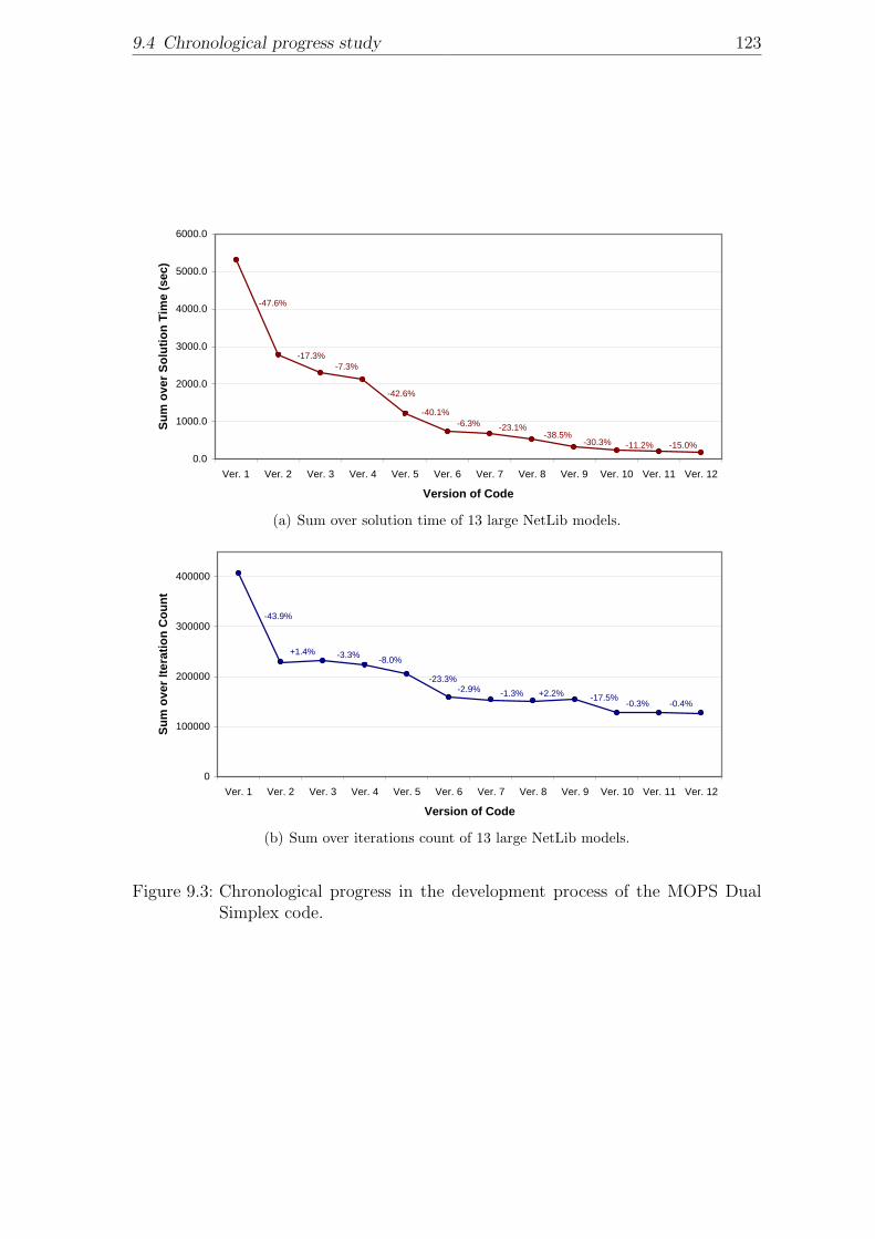
9.4 Chronological progress study 123
0.0
1000.0
2000.0
3000.0
4000.0
5000.0
6000.0
Ver. 1 Ver. 2 Ver. 3 Ver. 4 Ver. 5 Ver. 6 Ver. 7 Ver. 8 Ver. 9 Ver. 10 Ver. 11 Ver. 12
Version of Code
Sum
ove
r Sol
utio
n Ti
me
(sec
)
-47.6%
-11.2%-30.3%-38.5%
-23.1%-6.3%-40.1%
-42.6%
-7.3%-17.3%
-15.0%
(a) Sum over solution time of 13 large NetLib models.
0
100000
200000
300000
400000
Ver. 1 Ver. 2 Ver. 3 Ver. 4 Ver. 5 Ver. 6 Ver. 7 Ver. 8 Ver. 9 Ver. 10 Ver. 11 Ver. 12
Version of Code
Sum
ove
r Ite
ratio
n C
ount
-43.9%
-0.3%-17.5%+2.2%-1.3%-2.9%
-23.3%
-8.0%-3.3%+1.4%
-0.4%
(b) Sum over iterations count of 13 large NetLib models.
Figure 9.3: Chronological progress in the development process of the MOPS DualSimplex code.
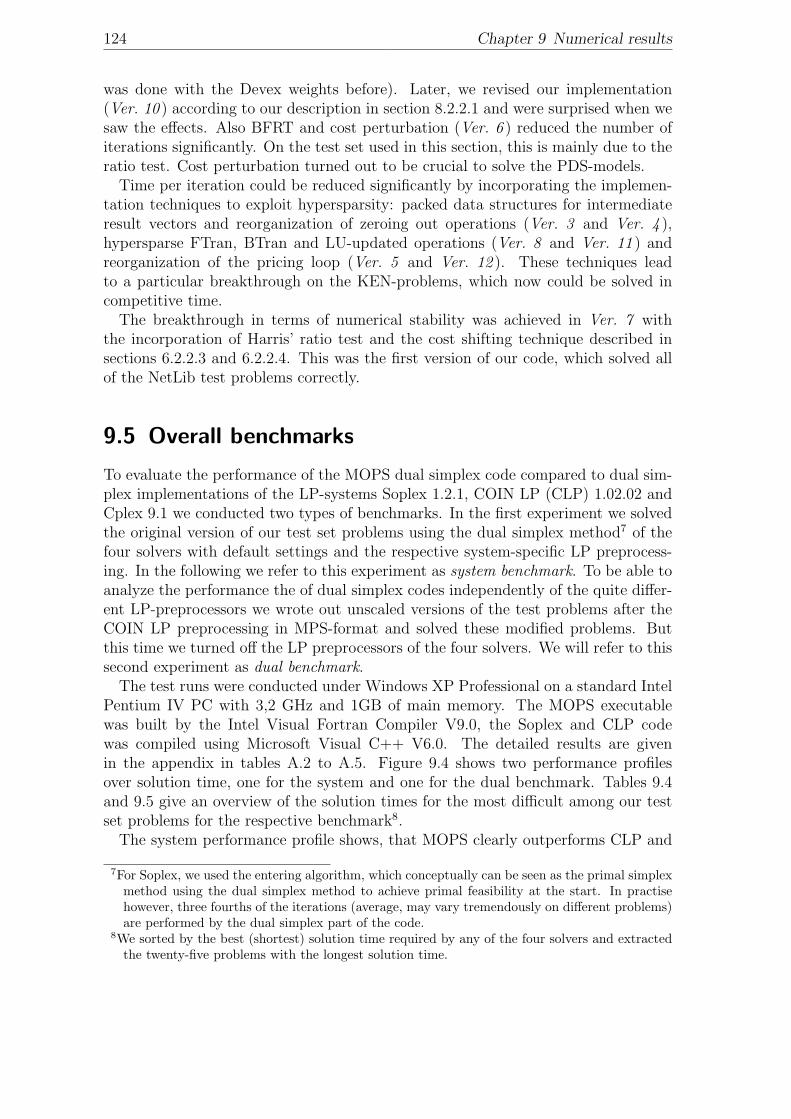
124 Chapter 9 Numerical results
was done with the Devex weights before). Later, we revised our implementation(Ver. 10 ) according to our description in section 8.2.2.1 and were surprised when wesaw the effects. Also BFRT and cost perturbation (Ver. 6 ) reduced the number ofiterations significantly. On the test set used in this section, this is mainly due to theratio test. Cost perturbation turned out to be crucial to solve the PDS-models.
Time per iteration could be reduced significantly by incorporating the implemen-tation techniques to exploit hypersparsity: packed data structures for intermediateresult vectors and reorganization of zeroing out operations (Ver. 3 and Ver. 4 ),hypersparse FTran, BTran and LU-updated operations (Ver. 8 and Ver. 11 ) andreorganization of the pricing loop (Ver. 5 and Ver. 12 ). These techniques leadto a particular breakthrough on the KEN-problems, which now could be solved incompetitive time.
The breakthrough in terms of numerical stability was achieved in Ver. 7 withthe incorporation of Harris’ ratio test and the cost shifting technique described insections 6.2.2.3 and 6.2.2.4. This was the first version of our code, which solved allof the NetLib test problems correctly.
9.5 Overall benchmarks
To evaluate the performance of the MOPS dual simplex code compared to dual sim-plex implementations of the LP-systems Soplex 1.2.1, COIN LP (CLP) 1.02.02 andCplex 9.1 we conducted two types of benchmarks. In the first experiment we solvedthe original version of our test set problems using the dual simplex method7 of thefour solvers with default settings and the respective system-specific LP preprocess-ing. In the following we refer to this experiment as system benchmark. To be able toanalyze the performance the of dual simplex codes independently of the quite differ-ent LP-preprocessors we wrote out unscaled versions of the test problems after theCOIN LP preprocessing in MPS-format and solved these modified problems. Butthis time we turned off the LP preprocessors of the four solvers. We will refer to thissecond experiment as dual benchmark.
The test runs were conducted under Windows XP Professional on a standard IntelPentium IV PC with 3,2 GHz and 1GB of main memory. The MOPS executablewas built by the Intel Visual Fortran Compiler V9.0, the Soplex and CLP codewas compiled using Microsoft Visual C++ V6.0. The detailed results are givenin the appendix in tables A.2 to A.5. Figure 9.4 shows two performance profilesover solution time, one for the system and one for the dual benchmark. Tables 9.4and 9.5 give an overview of the solution times for the most difficult among our testset problems for the respective benchmark8.
The system performance profile shows, that MOPS clearly outperforms CLP and
7For Soplex, we used the entering algorithm, which conceptually can be seen as the primal simplexmethod using the dual simplex method to achieve primal feasibility at the start. In practisehowever, three fourths of the iterations (average, may vary tremendously on different problems)are performed by the dual simplex part of the code.
8We sorted by the best (shortest) solution time required by any of the four solvers and extractedthe twenty-five problems with the longest solution time.
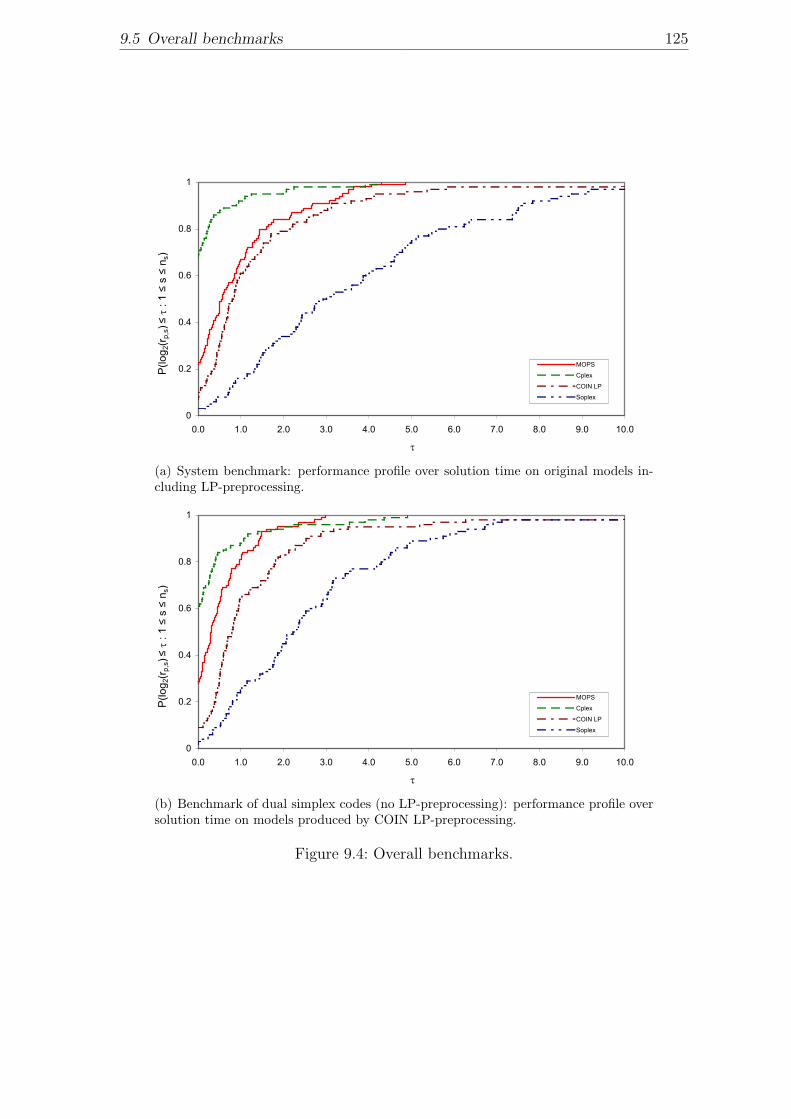
9.5 Overall benchmarks 125
0
0.2
0.4
0.6
0.8
1
0.0 1.0 2.0 3.0 4.0 5.0 6.0 7.0 8.0 9.0 10.0
MOPS
Cplex
COIN LP
Soplex
τ
P(lo
g 2(r p
,s) ≤
τ :
1 ≤
s ≤
n s)
(a) System benchmark: performance profile over solution time on original models in-cluding LP-preprocessing.
0
0.2
0.4
0.6
0.8
1
0.0 1.0 2.0 3.0 4.0 5.0 6.0 7.0 8.0 9.0 10.0
MOPS
Cplex
COIN LP
Soplex
τ
P(lo
g 2(r p
,s) ≤
τ :
1 ≤
s ≤
n s)
(b) Benchmark of dual simplex codes (no LP-preprocessing): performance profile oversolution time on models produced by COIN LP-preprocessing.
Figure 9.4: Overall benchmarks.
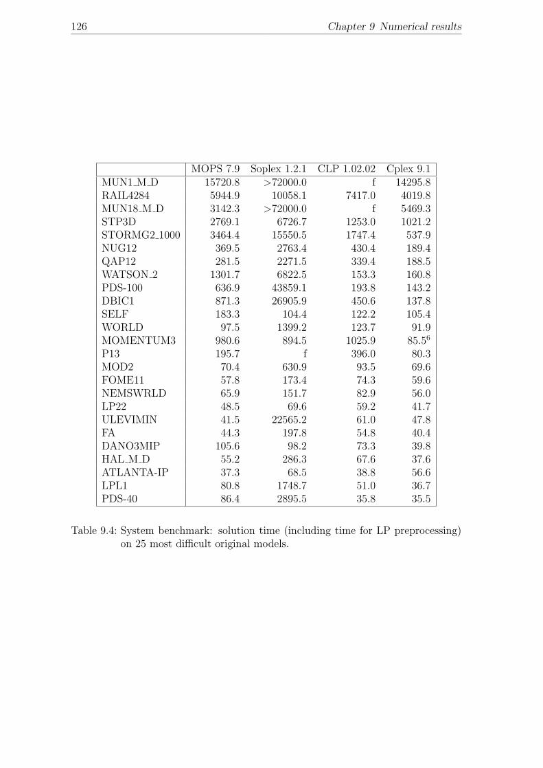
126 Chapter 9 Numerical results
MOPS 7.9 Soplex 1.2.1 CLP 1.02.02 Cplex 9.1MUN1 M D 15720.8 >72000.0 f 14295.8RAIL4284 5944.9 10058.1 7417.0 4019.8MUN18 M D 3142.3 >72000.0 f 5469.3STP3D 2769.1 6726.7 1253.0 1021.2STORMG2 1000 3464.4 15550.5 1747.4 537.9NUG12 369.5 2763.4 430.4 189.4QAP12 281.5 2271.5 339.4 188.5WATSON 2 1301.7 6822.5 153.3 160.8PDS-100 636.9 43859.1 193.8 143.2DBIC1 871.3 26905.9 450.6 137.8SELF 183.3 104.4 122.2 105.4WORLD 97.5 1399.2 123.7 91.9MOMENTUM3 980.6 894.5 1025.9 85.56
P13 195.7 f 396.0 80.3MOD2 70.4 630.9 93.5 69.6FOME11 57.8 173.4 74.3 59.6NEMSWRLD 65.9 151.7 82.9 56.0LP22 48.5 69.6 59.2 41.7ULEVIMIN 41.5 22565.2 61.0 47.8FA 44.3 197.8 54.8 40.4DANO3MIP 105.6 98.2 73.3 39.8HAL M D 55.2 286.3 67.6 37.6ATLANTA-IP 37.3 68.5 38.8 56.6LPL1 80.8 1748.7 51.0 36.7PDS-40 86.4 2895.5 35.8 35.5
Table 9.4: System benchmark: solution time (including time for LP preprocessing)on 25 most difficult original models.
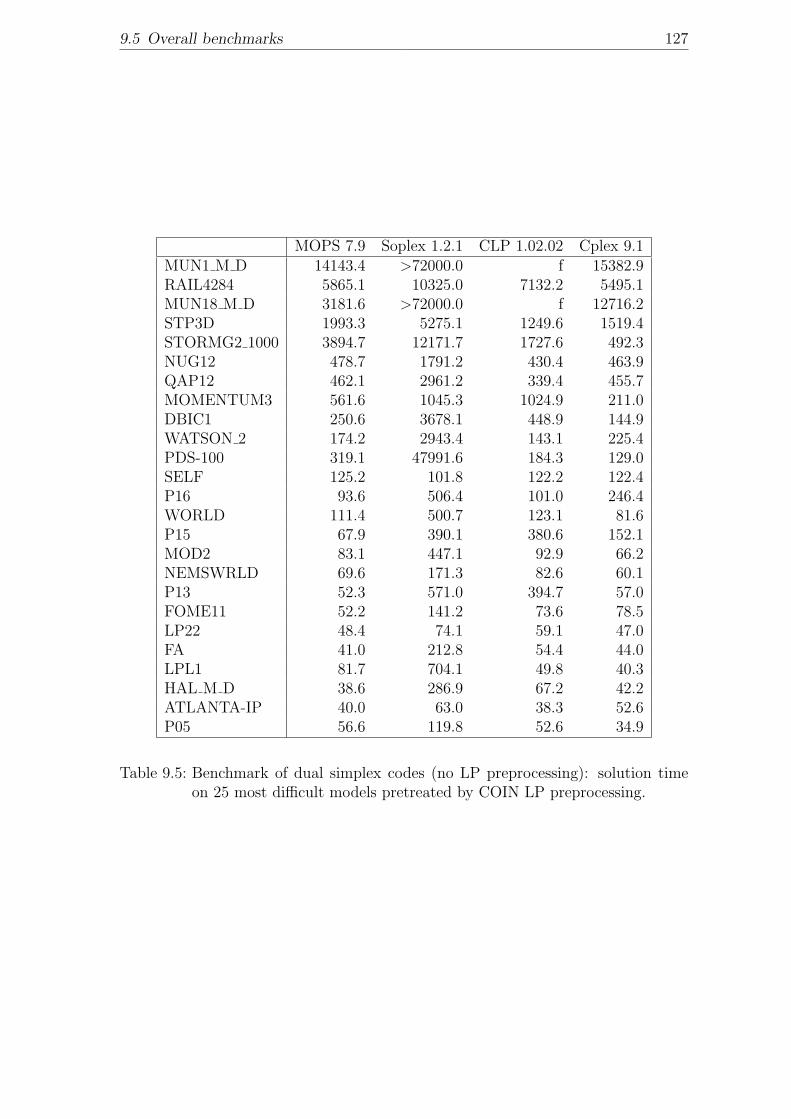
9.5 Overall benchmarks 127
MOPS 7.9 Soplex 1.2.1 CLP 1.02.02 Cplex 9.1MUN1 M D 14143.4 >72000.0 f 15382.9RAIL4284 5865.1 10325.0 7132.2 5495.1MUN18 M D 3181.6 >72000.0 f 12716.2STP3D 1993.3 5275.1 1249.6 1519.4STORMG2 1000 3894.7 12171.7 1727.6 492.3NUG12 478.7 1791.2 430.4 463.9QAP12 462.1 2961.2 339.4 455.7MOMENTUM3 561.6 1045.3 1024.9 211.0DBIC1 250.6 3678.1 448.9 144.9WATSON 2 174.2 2943.4 143.1 225.4PDS-100 319.1 47991.6 184.3 129.0SELF 125.2 101.8 122.2 122.4P16 93.6 506.4 101.0 246.4WORLD 111.4 500.7 123.1 81.6P15 67.9 390.1 380.6 152.1MOD2 83.1 447.1 92.9 66.2NEMSWRLD 69.6 171.3 82.6 60.1P13 52.3 571.0 394.7 57.0FOME11 52.2 141.2 73.6 78.5LP22 48.4 74.1 59.1 47.0FA 41.0 212.8 54.4 44.0LPL1 81.7 704.1 49.8 40.3HAL M D 38.6 286.9 67.2 42.2ATLANTA-IP 40.0 63.0 38.3 52.6P05 56.6 119.8 52.6 34.9
Table 9.5: Benchmark of dual simplex codes (no LP preprocessing): solution timeon 25 most difficult models pretreated by COIN LP preprocessing.

128 Chapter 9 Numerical results
Soplex, which both fail on two of the largest problems (MUN1 M D and MUN18 M D)9.On about 20% of the test models, MOPS achieves the best solution time. However,on this benchmark, Cplex 9.1 clearly yields the best overall performance. In the dualbenchmark however, MOPS achieves a better total solution time and is more stablewith respect to difficult problems. For about 30% of the problems it achieves thebest solution time and for about 80% of the problems it is at most two times slowerthan the best solver.
It is interesting to see, that MOPS and Soplex show significantly better results onthe problems pretreated by the COIN LP preprocessing, while the results of Cplex 9.1slightly worsen. Therefore we conclude, that great improvement of the performanceof the MOPS dual simplex code can be achieved by working on a better fine tuningof the MOPS LP preprocessing (which is however already quite sophisticated).
9CLP fails to remove the cost perturbation, Soplex exceeds the 12 hour time limit.
129
Chapter 10
Summary and Conclusion
In this thesis we presented the mathematical algorithms, computational techniquesand implementation details of our dual simplex code, which outperforms the bestexisting open-source and research codes and is competitive to the leading commercialLP-systems.
In part I we laid out the algorithmic basis for our implementation of the dualsimplex method, which is a classical two-phases approach. After introducing basicconcepts in chapter 2 we developed a new elaborate algorithmic description of thedual phase II in chapter 3, which incorporates the two crucial mathematical tech-niques ”dual steepest edge pricing” and ”bound flipping ratio test” into the reviseddual simplex algorithm. In chapter 4 we described several dual phase I methods. Weshowed, that the algorithmic approach to minimize the sum of dual infeasibilities canbe explicitly modeled as a subproblem, which is mathematically equivalent and candirectly be solved by the dual phase II. Therefore the subproblem approach is mucheasier to implement. Furthermore, we gave the first description of Pan’s dual phaseI method for general LPs with explicit lower and upper bounds. We overcame themain drawback of Pan’s method, which showed bad convergence on very few numer-ically rather difficult test problems, by combining it with the subproblem approach.The resulting algorithm outperformed the other methods in our computational tests.
In part II we gave detailed descriptions of techniques to achieve computationalefficiency and numerical stability. In chapter 5 we addressed the efficient solutionof the required systems of linear equations based on the LU-factorization of thebasis. To our knowledge we gave the first complete mathematical description of thistechnique, which allows to use only one instead of two permutation matrices in theFTran and BTran operations. Additionally, we discussed in detail, how the techniqueof Gilbert and Peierls [29] to exploit hypersparsity can be efficiently incorporated intothis solution framework. In chapter 6 we described techniques to solve numericallydifficult LP problems and reduce the number of degenerate iterations. Our maincontribution is the integration of Harris’ ratio test with bound flipping and costshifting techniques. We also gave a detailed description of the cost perturbationtechnique, which works well in our code.
In part III we discussed important implementation issues and presented compu-tational results. Chapter 8 focussed on the implementation of the dual pricing step,the dual ratio test and the exploitation of hypersparsity. The computational progressachieved by the presented techniques was analyzed in chapter 9. Furthermore, thischapter contained a study on the dual phase I and an overall benchmark study.
130 Chapter 10 Summary and Conclusion
We could show, that our new combined dual phase I approach outperforms othermethods from literature. We also studied the impact of the bound handling in LPpreprocessing on dual phase I and the overall performance. Finally, we compared theperformance of our code to that of the open-source codes COIN LP 1.02.02 and So-plex 1.2.1 and the commercial code Cplex 9.1. While it turned out to be significantlysuperior to Soplex and well better that COIN LP, it was slightly inferior to Cplex9.1. We want to emphasize again, that neither the techniques used in the COIN LPcode nor the internals of the Cplex code are documented in research literature.
Future research in this field can pursue several possible directions. One directionis to try to achieve further improvements in the given mathematical setting. Ofteninconspicuous implementation details have a great impact on the performance of thecode (like the bound handling after LP preprocessing). To discover and documentsuch details it is necessary to investigate the behavior of our dual simplex code onexceptionally difficult test problems. One important aspect is for instance to findbetter criteria, which allow for a problem specific switching between the differentcomputational techniques (dense, sparse, hypersparse linear systems; simple andbound flipping ratio test etc.). Another possible research direction is to improve thedual simplex algorithm on the mathematical side. For instance, Pan proposed a newpromising formulation of the dual simplex algorithm in [56]. It is however not clearyet, whether his algorithm is computationally competitive.
131
Bibliography
[1] Bpmpd test problems. http://www.sztaki.hu/∼meszaros/bpmpd/.
[2] Dsor test problems. http://dsor.upb.de/koberstein/lptestset/.
[3] Miplib 2003 test problems. http://miplib.zib.de/.
[4] Mittelmann test problems. ftp://plato.asu.edu/pub/lpfree.html.
[5] Netlib test problems. http://www.netlib.org/lp/data/.
[6] Sequential objectoriented simplex. http://www.zib.de/Optimization/Software/Soplex/,1996.
[7] O. Axelsson. A survey of preconditioned iterative methods for linear systems ofalgebraic equations. BIT, 25:166–187, 1985.
[8] R. H. Bartels and G. H. Golub. The simplex method of linear programmingusing lu decomposition. Commun. ACM, 12(5):266–268, 1969.
[9] M. Benichou, J. Gautier, G. Hentges, and G. Ribiere. The efficient solution oflarge-scale linear programming problems. Mathematical Programming, 13:280–322, 1977.
[10] R. Bixby. Solving real-world linear programs: a decade and more of progress.2002.
[11] R. E. Bixby and A. Martin. Parallelizing the dual simplex method. INFORMSJournal on Computing, 12(1):45–56, 2000.
[12] R. Bland. New finite pivot rule for the simplex method. Mathematics of Oper-ations Research, 2:103–107, 1977.
[13] R. K. Brayton, F. G. Gustavson, and R. A. Willoughby. Some results on sparsematrices. Mathematics of Computation, 24(122):937–954, 1970.
[14] A. L. Brearley, G. Mitra, and H. P. Williams. Analysis of mathematical pro-gramming problems prior to applying the simplex method. Mathematical Pro-gramming, 8:54–83, 1975.
[15] V. Chvatal. Linear Programming. W. H. Freeman and Company, New York,16th edition, 2002.
[16] L. Collatz and W. Wetterling. Optimierungsaufgaben. Springer-Verlag, Berlin,1966.
132 Bibliography
[17] W. H. Cunningham. Theoretical properties of the network simplex method.Mathematics of Operations Research, 4:196–208, 1979.
[18] G. B. Dantzig. Programming in a linear structure. U. S. Air Force Comptroller,USAF, Washington, D.C., 1948.
[19] G. B. Dantzig. Maximization of a linear function of variables subject to linearinequalities. In [40], pages 339–347.
[20] G. B. Dantzig and W. Orchard-Hays. The product form for the inverse in thesimplex method. Mathematical Tables and Other Aids toComputation, 8:64–67,1954.
[21] G. B. Dantzig, A. Orden, and P. Wolfe. The generalized simplex method forminimizing a linear form under linear inequality restraints. Pacific Journal ofMathematics, 5:183–195, 1955.
[22] E. D. Dolan and J. J. More. Benchmarking optimization software with perfor-mance profiles. Mathematical Programming, 91(2):201–213, 2002.
[23] I. S. Duff, A. M. Erisman, and J. K. Reid. Direct Methods for Sparse Matrices.Oxford University Press, Oxford, 1986.
[24] J. J. H. Forrest and J. A. Tomlin. Updating triangular factors of the basis tomaintain sparsity in the product form simplex method. Mathematical Program-ming, 2:263–278, 1972.
[25] J. J. H. Forrest and J. A. Tomlin. Implementing the simplex method for theoptimization subroutine library. IBM Systems Journal, 31(1):11–25, 1992.
[26] John J. Forrest and Donald Goldfarb. Steepest-edge simplex algorithms forlinear programming. Math. Program., 57(3):341–374, 1992.
[27] Robert Fourer. Notes on the dual simplex method. Draft report, 1994.
[28] S. I. Gass. The first linear-programming shoppe. Operations Research, 50(1):61–68, 2002.
[29] J. R. Gilbert and T. Peierls. Sparse partial pivoting in time proportional toarithmetic operations. SIAM J. Sci. Statist. Comput., 9:862–874, 1988.
[30] P. E. Gill, W. Murray, M. A. Saunders, and M. H. Wright. A practical anti-cycling procedure for linearly constrained optimization. Mathematical Program-ming, 45:437–474, 1989.
[31] P. E. Gill, W. Murray, and M. H. Wright. Numerical Linear Algebra and Opti-mization, volume 1. Addison-Wesley Publishing Company, 1991.
[32] G. H. Golub and C. F. Van Loan. Matrix Computations. The John HopkinsUniversity Press, Baltimore, London, 3 edition, 1996.
Bibliography 133
[33] P. M. J. Harris. Pivot selection methods of the DEVEX LP code. Math. Pro-gramming, 5:1–28, 1973.
[34] E. Hellermann and D. Rarick. Reinversion with the preassigned pivot procedure.Mathematical Programming, 1(2):195–215, 1971.
[35] A. Hoffman, M. Mannos, D. Sokolosky, and D. Wiegmann. Computationalexperience in solving linear programs. SIAM Journal, 1:1–33, 1953.
[36] A. J. Hoffman. Linear programming at the national bureau of standards. In[43].
[37] N. Kliewer, T. Mellouli, and L. Suhl. A time-space network based exact opti-mization model for multi-depot bus scheduling. European Journal of OperationsResearch, to appear 2005.
[38] A. Koberstein. Progress in the dual simplex algorithm for solving large scaleLP problems: Techniques for a fast and stable implementation. forthcoming.
[39] A. Koberstein and U.H. Suhl. Progress in the dual simplex algorithm for solv-ing large scale lp problems: Practical dual phase 1 algorithms. to appear in:Computational Optimization and Applications, 2005.
[40] T. C. Koopmans, editor. Activity Analysis of Production and Allocation, NewYork, 1951. John Wiley and Sons.
[41] E. Kostina. The long step rule in the bounded-variable dual simplex method:Numerical experiments. Mathematical Methods of Operations Research, 55:413–429, 2002.
[42] C. E. Lemke. The dual method of solving the linear programming problem.Naval Research Logistics Quarterly, 1:36–47, 1954.
[43] J. K. Lenstra, A. H. G. Rinnooy Kan, and A. Schrijver, editors. History ofMathematical Programming. North-Holland, Amsterdam, 1991.
[44] R. Lougee-Heimer, F. Barahona, B. Dietrich, J. P. Fasano, J. J. Forrest,R. Harder, L. Ladanyi, T. Pfender, T. Ralphs, M. Saltzman, and K. Schien-berger. The coin-or initiative: Open-source software accelerates operations re-search progress. ORMS Today, 28(5):20–22, October 2001.
[45] H. M. Markowitz. The elimination form of the inverse and its applications tolinear programming. Management Science, 3:255–269, 1957.
[46] I. Maros. Computational techniques of the simplex method. Kluwer’s Interna-tional Series, 2003.
[47] I. Maros. A generalized dual phase-2 simplex algorithm. European Journal ofOperational Research, 149(1):1–16, 2003.
134 Bibliography
[48] I. Maros. A piecewise linear dual phase-1 algorithm for the simplex method withall types of variables. Computational Optimization and Applications, 26:63–81,2003.
[49] C. Meszaros and U. H. Suhl. Advanced preprocessing techniques for linear andquadratic programming. OR Spectrum, 25(4):575–595, 2003.
[50] B. A. Murtagh. Advanced Linear Programming: Computation and Practice.McGraw-Hill, INC., 1981.
[51] W. Orchard-Hays. History of the development of lp solvers. Interfaces, 20(4):61–73, July-August 1990.
[52] A. Orden. Solution of systems of linear inequalities on a digital computer.Proceedings of the meeting of the ACM, May 2, 1952, Pittsburgh, PA, 1952. Di-rectorate of Management Analysis, Headquarters, U.S. Air Force, Washington,D.C.
[53] M. W. Padberg. Linear optimization and extensions. Springer, Berlin, 1995.
[54] P. Q. Pan. Practical finite pivoting rules for the simplex method. OR Spektrum,12:219–225, 1990.
[55] P. Q. Pan. The most-obtuse-angle row pivot rule for achieving dual feasibility:a computational study. European Journal of Operations Research, 101(1):167–176, 1997.
[56] P. Q. Pan. A revised dual projective pivot algorithm for linear programming.2004.
[57] F.M. Kirillova R. Gabasov and O.I. Kostyukova. A method of solving generallinear programming problems. Doklady AN BSSR, 23(3):197–200, 1979. (inRussian).
[58] J. K. Reid. A sparsity-exploiting variant of the bartels-golub decomposition forlinear programming bases. Mathematical Programming, 24:55–69, 1982.
[59] D. Ryan and M. Osborne. On the solution of highly degenerate linear pro-grammes. Mathematical Programming, 41:385–392, 1988.
[60] M. A. Saunders. The complexity of computational problem solving, chapter Thecomplexity of LU updating in the simplex method, pages 214–230. Universityof Queensland Press, St. Lucia, Queensland, 1976.
[61] M. A. Saunders. Sparse Matrix Computations, chapter A fast, stable implemen-tation of the simplex method using Bartels-Golub updating, pages 213–226.Academic Press, New York et. al., 1976.
[62] I. Steinzen, A. Koberstein, and U.H. Suhl. Ein entscheidungsunterstutzungssys-tem zur zuschnittoptimierung von rollenstahl. In [64], pages 126–143.
Bibliography 135
[63] L. M. Suhl and U. H. Suhl. A fast lu-update for linear programming. Annalsof Operations Research, 43:33–47, 1993.
[64] L. M. Suhl and S. Voss, editors. Quantitative Methoden in ERP und SCM,DSOR Beitrage zur Wirtschaftsinformatik. 2004.
[65] U. H. Suhl. Mops - mathematical optimization system. European Journal ofOperational Research, 72:312–322, 1994.
[66] U. H. Suhl. Mops - mathematical optimization system. OR News, 8:11–16,2000.
[67] U. H. Suhl. It-gestutzte, operative sortimentsplanung. In B. Jahnke and F. Wall,editors, IT-gestutzte betriebliche Entscheidungsprozesse, pages 175–194. Gabler,2001.
[68] U. H. Suhl and L. M. Suhl. Computing sparse lu factorizations for large-scalelinear programming bases. ORSA Journal on Computing, 2(4):325–335, 1990.
[69] U. H. Suhl and L. M. Suhl. Operational Research in Industry, chapter SolvingAirline Fleet Scheduling Problems with Mixed-Integer Programming, pages 135–156. MacMillan Press Ltd., 1999.
[70] U. H. Suhl and R. Szymanski. Supernode processing of mixed-integer models.Computational Optimization and Applications, 3:317–331, 1994.
[71] U. H. Suhl and V. Waue. Fortschritte bei der losung gemischt-ganzzahligeroptimierungsmodelle. In [64], pages 35–53.
[72] R. P. Tewarson. The product form of inverses of sparse matrices and graphtheory. SIAM Review, 9(1):91–99, 1967.
[73] J. A. Tomlin. On scaling linear programming problems. In M. L. Balinski andE. Hellerman, editors, Computational Practise in Mathematical Programming,chapter Mathematical Programming Study 4, pages 146–166. North-Holland,Amsterdam, 1975.
[74] P. Wolfe. The composite simplex algorithm. SIAM Review, 7(1):42–54, 1965.
[75] R. Wunderling. Paralleler und objektorientierter simplex. Technical report,Konrad-Zuse-Zentrum fur Informationstechnik Berlin, 1996.

136 Bibliography

137
Appendix A
Tables
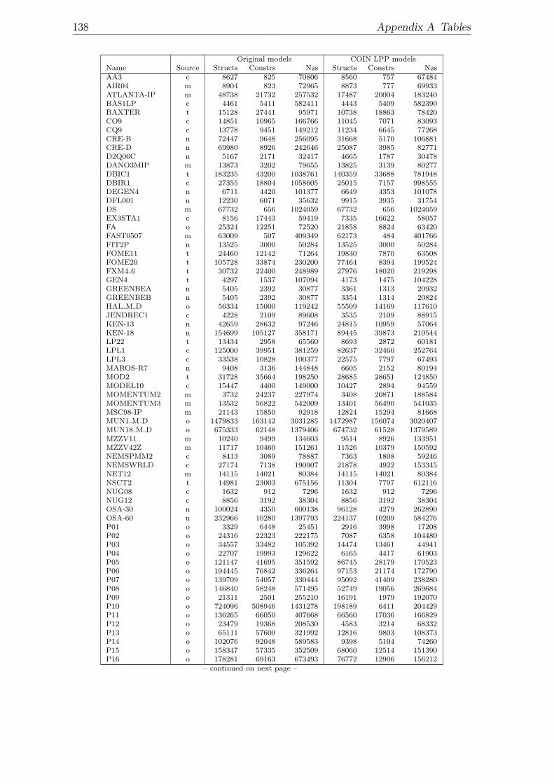
138 Appendix A Tables
Original models COIN LPP modelsName Source Structs Constrs Nzs Structs Constrs NzsAA3 c 8627 825 70806 8560 757 67484AIR04 m 8904 823 72965 8873 777 69933ATLANTA-IP m 48738 21732 257532 17487 20004 183240BAS1LP c 4461 5411 582411 4443 5409 582390BAXTER t 15128 27441 95971 10738 18863 78420CO9 c 14851 10965 166766 11045 7071 83093CQ9 c 13778 9451 149212 11234 6645 77268CRE-B n 72447 9648 256095 31668 5170 106881CRE-D n 69980 8926 242646 25087 3985 82771D2Q06C n 5167 2171 32417 4665 1787 30478DANO3MIP m 13873 3202 79655 13825 3139 80277DBIC1 t 183235 43200 1038761 140359 33688 781948DBIR1 c 27355 18804 1058605 25015 7157 998555DEGEN4 n 6711 4420 101377 6649 4353 101078DFL001 n 12230 6071 35632 9915 3935 31754DS m 67732 656 1024059 67732 656 1024059EX3STA1 c 8156 17443 59419 7335 16622 58057FA o 25324 12251 72520 21858 8824 63420FAST0507 m 63009 507 409349 62173 484 401766FIT2P n 13525 3000 50284 13525 3000 50284FOME11 t 24460 12142 71264 19830 7870 63508FOME20 t 105728 33874 230200 77464 8394 199524FXM4 6 t 30732 22400 248989 27976 18020 219298GEN4 t 4297 1537 107094 4173 1475 104228GREENBEA n 5405 2392 30877 3361 1313 20932GREENBEB n 5405 2392 30877 3354 1314 20824HAL M D o 56334 15000 119242 55509 14169 117610JENDREC1 c 4228 2109 89608 3535 2109 88915KEN-13 n 42659 28632 97246 24815 10959 57064KEN-18 n 154699 105127 358171 89445 39873 210544LP22 t 13434 2958 65560 8693 2872 60181LPL1 c 125000 39951 381259 82637 32460 252764LPL3 c 33538 10828 100377 22575 7797 67493MAROS-R7 n 9408 3136 144848 6605 2152 80194MOD2 t 31728 35664 198250 28685 28651 124850MODEL10 c 15447 4400 149000 10427 2894 94559MOMENTUM2 m 3732 24237 227974 3408 20871 188584MOMENTUM3 m 13532 56822 542009 13401 56490 541035MSC98-IP m 21143 15850 92918 12824 15294 81668MUN1 M D o 1479833 163142 3031285 1472987 156074 3020407MUN18 M D o 675333 62148 1379406 674732 61528 1379589MZZV11 m 10240 9499 134603 9514 8926 133951MZZV42Z m 11717 10460 151261 11526 10379 150592NEMSPMM2 c 8413 3089 78887 7363 1808 59246NEMSWRLD c 27174 7138 190907 21878 4922 153345NET12 m 14115 14021 80384 14115 14021 80384NSCT2 t 14981 23003 675156 11304 7797 612116NUG08 c 1632 912 7296 1632 912 7296NUG12 c 8856 3192 38304 8856 3192 38304OSA-30 n 100024 4350 600138 96128 4279 262890OSA-60 n 232966 10280 1397793 224137 10209 584276P01 o 3329 6448 25451 2916 3998 17208P02 o 24316 22323 222175 7087 6358 104480P03 o 34557 33482 105392 14474 13461 44941P04 o 22707 19993 129622 6165 4417 61903P05 o 121147 41695 351592 86745 28179 170523P06 o 194445 76842 336264 97153 21174 172790P07 o 139709 54057 330444 95092 41409 238280P08 o 146840 58248 571495 52749 19056 269684P09 o 21311 2501 255210 16191 1979 192070P10 o 724096 508946 1431278 198189 6411 204429P11 o 136265 66050 407668 66560 17036 166829P12 o 23479 19368 208530 4583 3214 68332P13 o 65111 57600 321992 12816 9803 108373P14 o 102076 92048 589583 9398 5104 74260P15 o 158347 57335 352509 68060 12514 151390P16 o 178281 69163 673493 76772 12906 156212
– continued on next page –
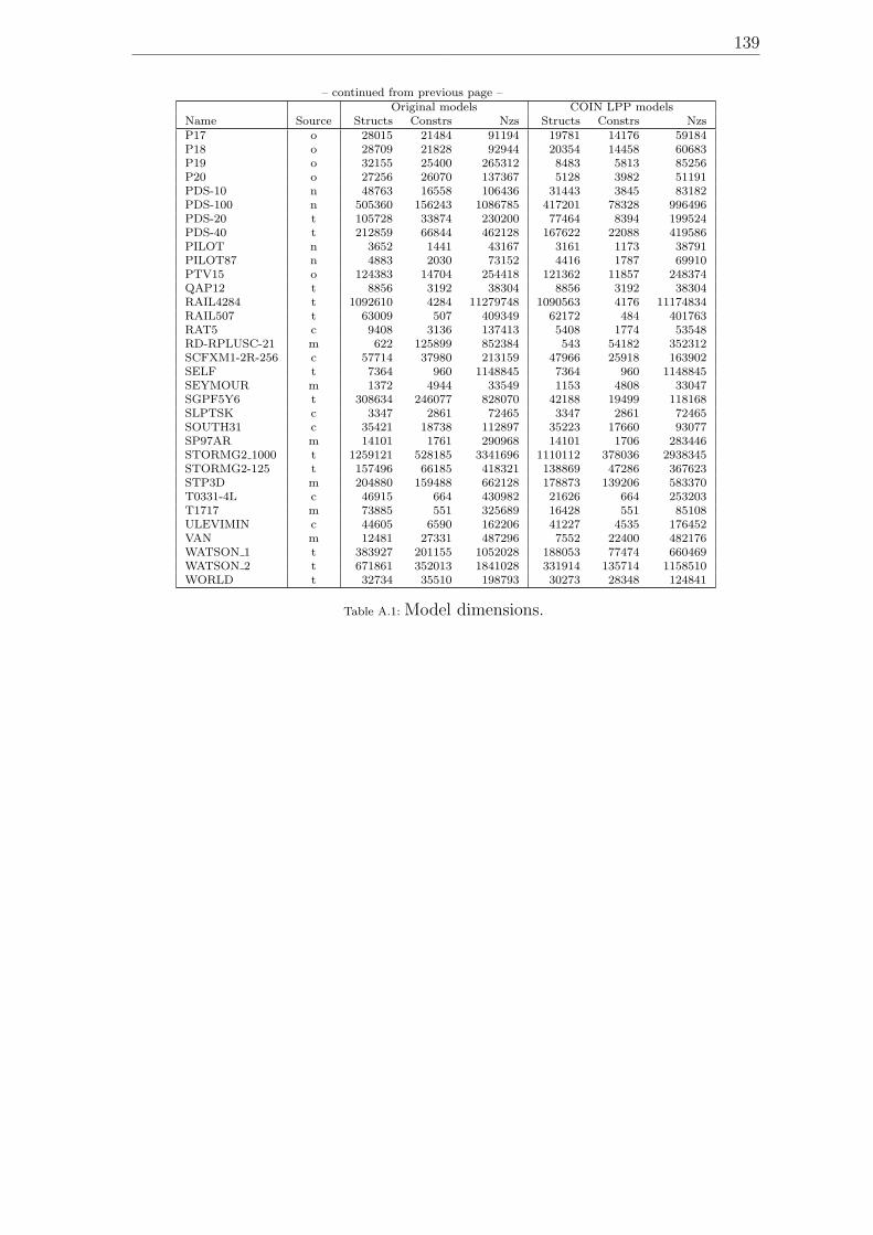
139
– continued from previous page –Original models COIN LPP models
Name Source Structs Constrs Nzs Structs Constrs NzsP17 o 28015 21484 91194 19781 14176 59184P18 o 28709 21828 92944 20354 14458 60683P19 o 32155 25400 265312 8483 5813 85256P20 o 27256 26070 137367 5128 3982 51191PDS-10 n 48763 16558 106436 31443 3845 83182PDS-100 n 505360 156243 1086785 417201 78328 996496PDS-20 t 105728 33874 230200 77464 8394 199524PDS-40 t 212859 66844 462128 167622 22088 419586PILOT n 3652 1441 43167 3161 1173 38791PILOT87 n 4883 2030 73152 4416 1787 69910PTV15 o 124383 14704 254418 121362 11857 248374QAP12 t 8856 3192 38304 8856 3192 38304RAIL4284 t 1092610 4284 11279748 1090563 4176 11174834RAIL507 t 63009 507 409349 62172 484 401763RAT5 c 9408 3136 137413 5408 1774 53548RD-RPLUSC-21 m 622 125899 852384 543 54182 352312SCFXM1-2R-256 c 57714 37980 213159 47966 25918 163902SELF t 7364 960 1148845 7364 960 1148845SEYMOUR m 1372 4944 33549 1153 4808 33047SGPF5Y6 t 308634 246077 828070 42188 19499 118168SLPTSK c 3347 2861 72465 3347 2861 72465SOUTH31 c 35421 18738 112897 35223 17660 93077SP97AR m 14101 1761 290968 14101 1706 283446STORMG2 1000 t 1259121 528185 3341696 1110112 378036 2938345STORMG2-125 t 157496 66185 418321 138869 47286 367623STP3D m 204880 159488 662128 178873 139206 583370T0331-4L c 46915 664 430982 21626 664 253203T1717 m 73885 551 325689 16428 551 85108ULEVIMIN c 44605 6590 162206 41227 4535 176452VAN m 12481 27331 487296 7552 22400 482176WATSON 1 t 383927 201155 1052028 188053 77474 660469WATSON 2 t 671861 352013 1841028 331914 135714 1158510WORLD t 32734 35510 198793 30273 28348 124841
Table A.1: Model dimensions.
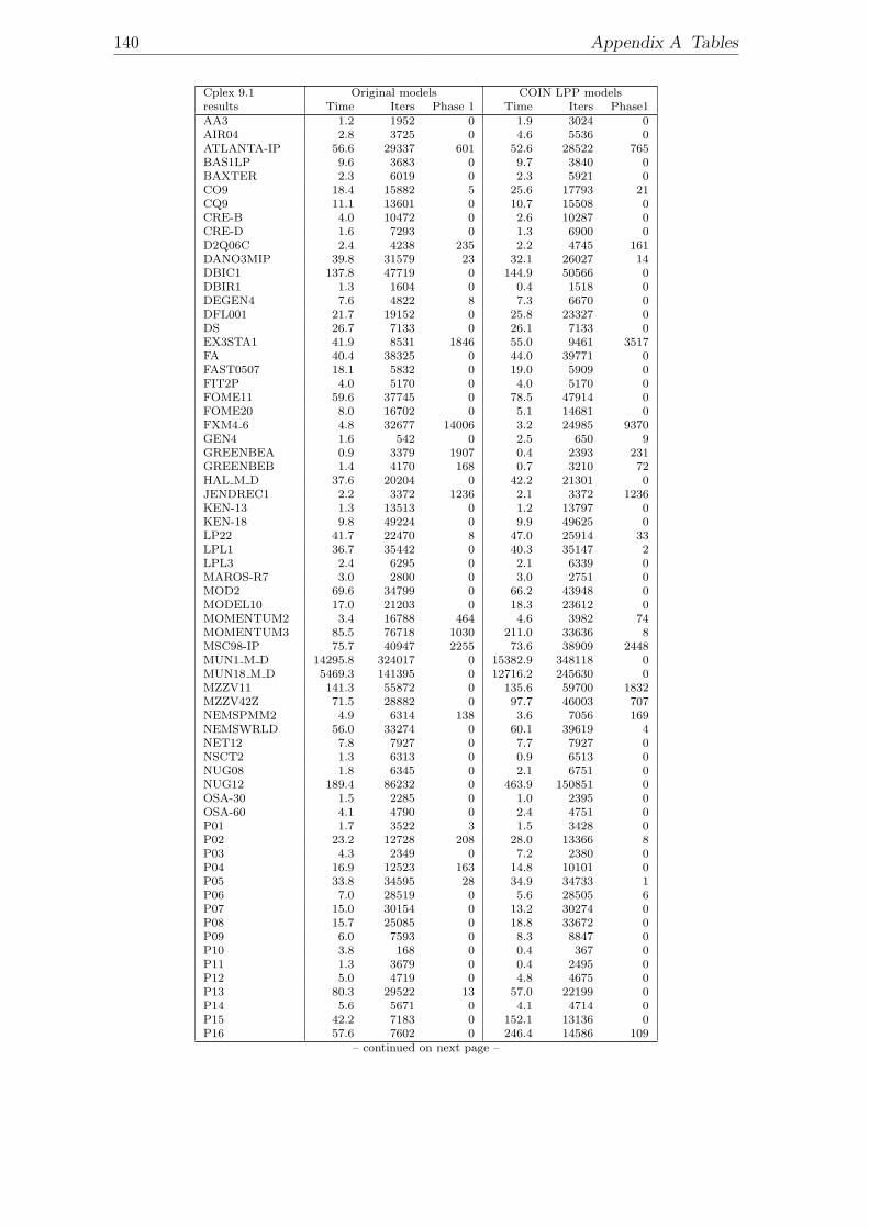
140 Appendix A Tables
Cplex 9.1 Original models COIN LPP modelsresults Time Iters Phase 1 Time Iters Phase1AA3 1.2 1952 0 1.9 3024 0AIR04 2.8 3725 0 4.6 5536 0ATLANTA-IP 56.6 29337 601 52.6 28522 765BAS1LP 9.6 3683 0 9.7 3840 0BAXTER 2.3 6019 0 2.3 5921 0CO9 18.4 15882 5 25.6 17793 21CQ9 11.1 13601 0 10.7 15508 0CRE-B 4.0 10472 0 2.6 10287 0CRE-D 1.6 7293 0 1.3 6900 0D2Q06C 2.4 4238 235 2.2 4745 161DANO3MIP 39.8 31579 23 32.1 26027 14DBIC1 137.8 47719 0 144.9 50566 0DBIR1 1.3 1604 0 0.4 1518 0DEGEN4 7.6 4822 8 7.3 6670 0DFL001 21.7 19152 0 25.8 23327 0DS 26.7 7133 0 26.1 7133 0EX3STA1 41.9 8531 1846 55.0 9461 3517FA 40.4 38325 0 44.0 39771 0FAST0507 18.1 5832 0 19.0 5909 0FIT2P 4.0 5170 0 4.0 5170 0FOME11 59.6 37745 0 78.5 47914 0FOME20 8.0 16702 0 5.1 14681 0FXM4 6 4.8 32677 14006 3.2 24985 9370GEN4 1.6 542 0 2.5 650 9GREENBEA 0.9 3379 1907 0.4 2393 231GREENBEB 1.4 4170 168 0.7 3210 72HAL M D 37.6 20204 0 42.2 21301 0JENDREC1 2.2 3372 1236 2.1 3372 1236KEN-13 1.3 13513 0 1.2 13797 0KEN-18 9.8 49224 0 9.9 49625 0LP22 41.7 22470 8 47.0 25914 33LPL1 36.7 35442 0 40.3 35147 2LPL3 2.4 6295 0 2.1 6339 0MAROS-R7 3.0 2800 0 3.0 2751 0MOD2 69.6 34799 0 66.2 43948 0MODEL10 17.0 21203 0 18.3 23612 0MOMENTUM2 3.4 16788 464 4.6 3982 74MOMENTUM3 85.5 76718 1030 211.0 33636 8MSC98-IP 75.7 40947 2255 73.6 38909 2448MUN1 M D 14295.8 324017 0 15382.9 348118 0MUN18 M D 5469.3 141395 0 12716.2 245630 0MZZV11 141.3 55872 0 135.6 59700 1832MZZV42Z 71.5 28882 0 97.7 46003 707NEMSPMM2 4.9 6314 138 3.6 7056 169NEMSWRLD 56.0 33274 0 60.1 39619 4NET12 7.8 7927 0 7.7 7927 0NSCT2 1.3 6313 0 0.9 6513 0NUG08 1.8 6345 0 2.1 6751 0NUG12 189.4 86232 0 463.9 150851 0OSA-30 1.5 2285 0 1.0 2395 0OSA-60 4.1 4790 0 2.4 4751 0P01 1.7 3522 3 1.5 3428 0P02 23.2 12728 208 28.0 13366 8P03 4.3 2349 0 7.2 2380 0P04 16.9 12523 163 14.8 10101 0P05 33.8 34595 28 34.9 34733 1P06 7.0 28519 0 5.6 28505 6P07 15.0 30154 0 13.2 30274 0P08 15.7 25085 0 18.8 33672 0P09 6.0 7593 0 8.3 8847 0P10 3.8 168 0 0.4 367 0P11 1.3 3679 0 0.4 2495 0P12 5.0 4719 0 4.8 4675 0P13 80.3 29522 13 57.0 22199 0P14 5.6 5671 0 4.1 4714 0P15 42.2 7183 0 152.1 13136 0P16 57.6 7602 0 246.4 14586 109
– continued on next page –
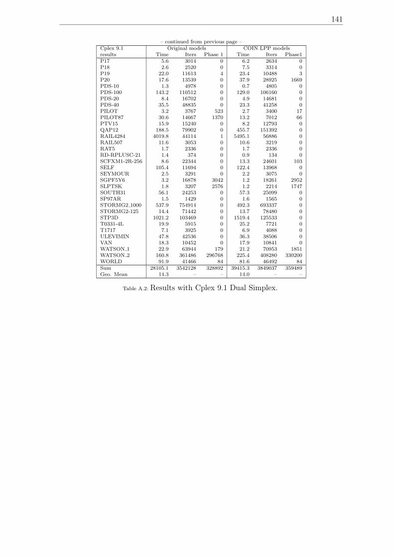
141
– continued from previous page –Cplex 9.1 Original models COIN LPP modelsresults Time Iters Phase 1 Time Iters Phase1P17 5.6 3014 0 6.2 2634 0P18 2.6 2520 0 7.5 3314 0P19 22.0 11613 4 23.4 10488 3P20 17.6 13539 0 37.9 28925 1669PDS-10 1.3 4978 0 0.7 4805 0PDS-100 143.2 110512 0 129.0 106160 0PDS-20 8.4 16702 0 4.9 14681 0PDS-40 35.5 48835 0 23.3 41258 0PILOT 3.2 3767 523 2.7 3400 17PILOT87 30.6 14667 1370 13.2 7012 66PTV15 15.9 15240 0 8.2 12793 0QAP12 188.5 79902 0 455.7 151392 0RAIL4284 4019.8 44114 1 5495.1 56886 0RAIL507 11.6 3053 0 10.6 3219 0RAT5 1.7 2336 0 1.7 2336 0RD-RPLUSC-21 1.4 374 0 0.9 134 0SCFXM1-2R-256 8.6 22344 0 13.3 24601 103SELF 105.4 11694 0 122.4 13968 0SEYMOUR 2.5 3291 0 2.2 3075 0SGPF5Y6 3.2 16878 3042 1.2 18261 2952SLPTSK 1.8 3207 2576 1.2 2214 1747SOUTH31 56.1 24253 0 57.3 25099 0SP97AR 1.5 1429 0 1.6 1565 0STORMG2 1000 537.9 754914 0 492.3 693337 0STORMG2-125 14.4 71442 0 13.7 78480 0STP3D 1021.2 103469 0 1519.4 125533 0T0331-4L 19.9 5915 0 25.2 7721 0T1717 7.1 3925 0 6.9 4088 0ULEVIMIN 47.8 42536 0 36.3 38506 0VAN 18.3 10452 0 17.9 10841 0WATSON 1 22.9 63944 179 21.2 70953 1851WATSON 2 160.8 361486 296768 225.4 408280 330200WORLD 91.9 41466 84 81.6 46492 84Sum 28105.1 3542128 328892 39415.3 3849037 359489Geo. Mean 14.3 – – 14.0 – –
Table A.2: Results with Cplex 9.1 Dual Simplex.
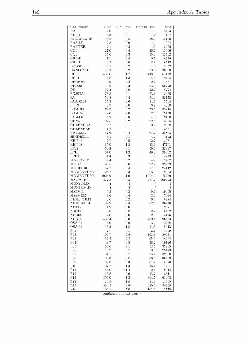
142 Appendix A Tables
CLP results Time PP Time Time in Dual ItersAA3 2.0 0.1 1.9 2423AIR04 4.3 0.1 4.2 4107ATLANTA-IP 38.8 0.5 38.3 15190BAS1LP 2.8 0.9 1.9 1094BAXTER 2.1 0.2 1.9 3952CO9 27.0 0.4 26.6 13996CQ9 15.6 0.3 15.3 12502CRE-B 7.1 0.4 6.7 8928CRE-D 4.5 0.6 3.9 6513D2Q06C 4.5 0.2 4.3 5842DANO3MIP 73.3 0.2 73.1 30850DBIC1 450.6 1.7 448.9 51128DBIR1 5.8 1.3 4.5 2424DEGEN4 9.9 0.2 9.7 7557DFL001 33.6 0.3 33.3 22270DS 32.3 0.0 32.3 5724EX3STA1 73.8 0.1 73.6 12455FA 54.8 0.4 54.4 38178FAST0507 15.3 0.6 14.7 3504FIT2P 6.9 0.0 6.9 4830FOME11 74.3 0.7 73.6 39414FOME20 9.0 2.0 7.0 13759FXM4 6 4.9 0.8 4.2 19150GEN4 92.5 0.2 92.3 3855GREENBEA 0.7 0.1 0.6 2398GREENBEB 1.2 0.1 1.1 3637HAL M D 67.6 0.4 67.2 25863JENDREC1 4.1 0.1 4.0 4142KEN-13 2.7 0.5 2.2 13031KEN-18 15.0 1.8 13.3 47761LP22 59.2 0.1 59.1 22327LPL1 51.0 1.2 49.8 28832LPL3 1.4 0.3 1.2 4249MAROS-R7 4.4 0.2 4.2 2467MOD2 93.5 0.6 92.9 33269MODEL10 37.7 0.4 37.3 24112MOMENTUM2 26.7 0.3 26.3 9933MOMENTUM3 1025.9 1.0 1024.9 75259MSC98-IP 277.5 0.3 277.2 100222MUN1 M D f f f fMUN18 M D f f f fMZZV11 9.3 0.3 9.0 10495MZZV42Z 3.6 0.4 3.3 7044NEMSPMM2 6.6 0.2 6.4 8974NEMSWRLD 82.9 0.4 82.6 36940NET12 1.9 0.0 1.9 2071NSCT2 3.0 0.8 2.2 5482NUG08 2.0 0.0 2.0 4126NUG12 430.4 0.0 430.4 96853OSA-30 4.0 0.9 3.1 2258OSA-60 13.3 1.8 11.5 5013P01 2.7 0.1 2.6 4059P02 103.7 0.8 102.9 30581P03 65.3 0.3 65.0 16924P04 48.7 0.5 48.2 19126P05 54.6 2.1 52.6 33935P06 13.2 3.7 9.5 29179P07 31.1 5.7 25.4 39590P08 39.3 2.8 36.5 36509P09 32.0 0.3 31.7 15379P10 107.7 91.3 16.4 7251P11 54.0 51.4 2.6 9914P12 13.8 0.6 13.2 8311P13 396.0 1.3 394.7 61403P14 15.9 1.9 14.0 11955P15 384.3 3.8 380.6 59969P16 106.1 5.0 101.0 13775
– continued on next page –
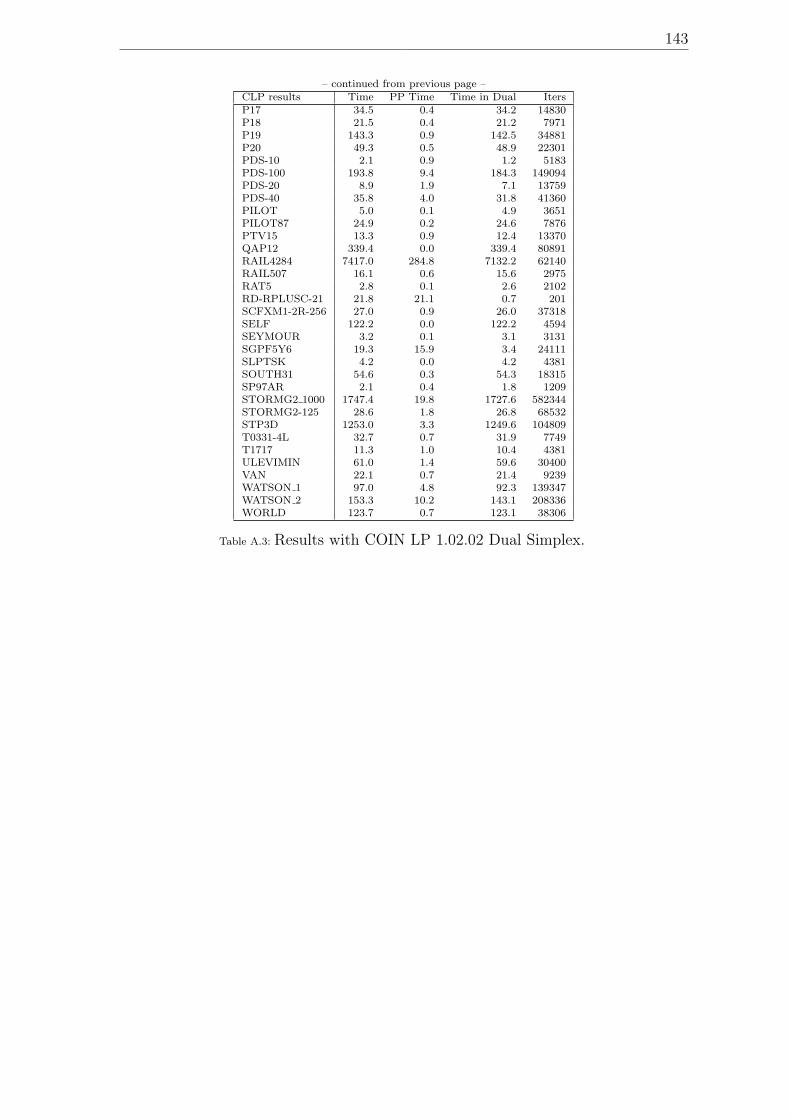
143
– continued from previous page –CLP results Time PP Time Time in Dual ItersP17 34.5 0.4 34.2 14830P18 21.5 0.4 21.2 7971P19 143.3 0.9 142.5 34881P20 49.3 0.5 48.9 22301PDS-10 2.1 0.9 1.2 5183PDS-100 193.8 9.4 184.3 149094PDS-20 8.9 1.9 7.1 13759PDS-40 35.8 4.0 31.8 41360PILOT 5.0 0.1 4.9 3651PILOT87 24.9 0.2 24.6 7876PTV15 13.3 0.9 12.4 13370QAP12 339.4 0.0 339.4 80891RAIL4284 7417.0 284.8 7132.2 62140RAIL507 16.1 0.6 15.6 2975RAT5 2.8 0.1 2.6 2102RD-RPLUSC-21 21.8 21.1 0.7 201SCFXM1-2R-256 27.0 0.9 26.0 37318SELF 122.2 0.0 122.2 4594SEYMOUR 3.2 0.1 3.1 3131SGPF5Y6 19.3 15.9 3.4 24111SLPTSK 4.2 0.0 4.2 4381SOUTH31 54.6 0.3 54.3 18315SP97AR 2.1 0.4 1.8 1209STORMG2 1000 1747.4 19.8 1727.6 582344STORMG2-125 28.6 1.8 26.8 68532STP3D 1253.0 3.3 1249.6 104809T0331-4L 32.7 0.7 31.9 7749T1717 11.3 1.0 10.4 4381ULEVIMIN 61.0 1.4 59.6 30400VAN 22.1 0.7 21.4 9239WATSON 1 97.0 4.8 92.3 139347WATSON 2 153.3 10.2 143.1 208336WORLD 123.7 0.7 123.1 38306
Table A.3: Results with COIN LP 1.02.02 Dual Simplex.
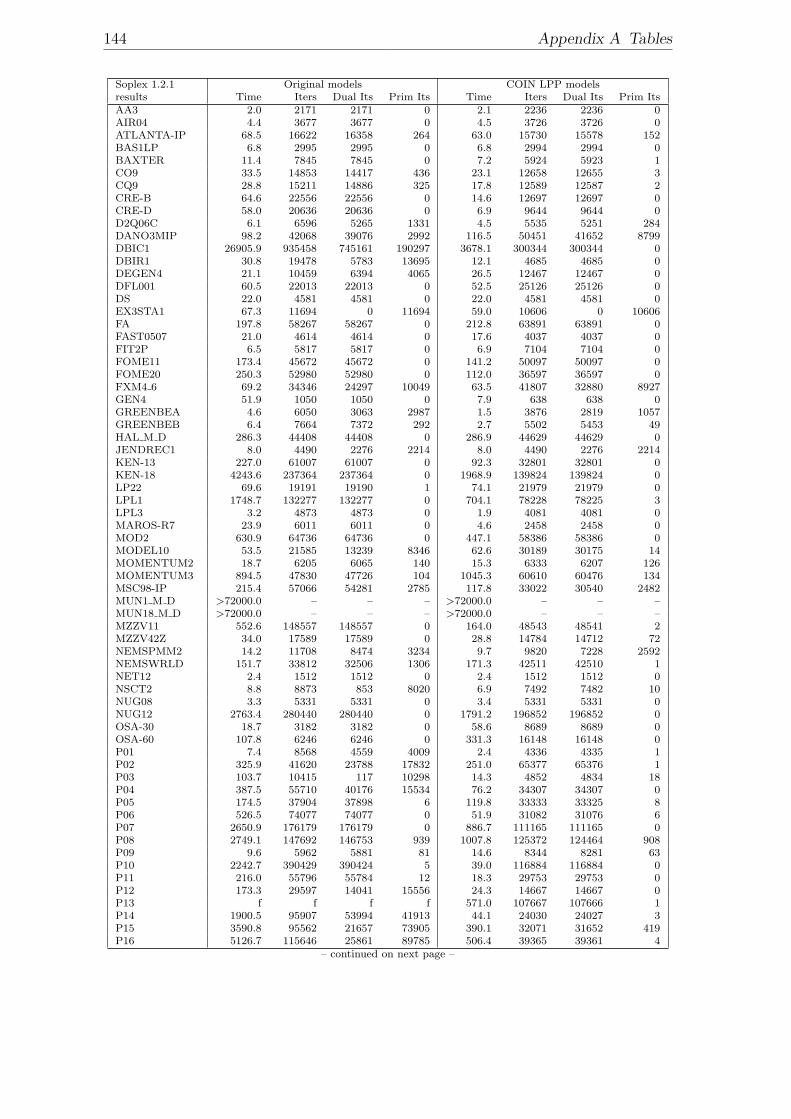
144 Appendix A Tables
Soplex 1.2.1 Original models COIN LPP modelsresults Time Iters Dual Its Prim Its Time Iters Dual Its Prim ItsAA3 2.0 2171 2171 0 2.1 2236 2236 0AIR04 4.4 3677 3677 0 4.5 3726 3726 0ATLANTA-IP 68.5 16622 16358 264 63.0 15730 15578 152BAS1LP 6.8 2995 2995 0 6.8 2994 2994 0BAXTER 11.4 7845 7845 0 7.2 5924 5923 1CO9 33.5 14853 14417 436 23.1 12658 12655 3CQ9 28.8 15211 14886 325 17.8 12589 12587 2CRE-B 64.6 22556 22556 0 14.6 12697 12697 0CRE-D 58.0 20636 20636 0 6.9 9644 9644 0D2Q06C 6.1 6596 5265 1331 4.5 5535 5251 284DANO3MIP 98.2 42068 39076 2992 116.5 50451 41652 8799DBIC1 26905.9 935458 745161 190297 3678.1 300344 300344 0DBIR1 30.8 19478 5783 13695 12.1 4685 4685 0DEGEN4 21.1 10459 6394 4065 26.5 12467 12467 0DFL001 60.5 22013 22013 0 52.5 25126 25126 0DS 22.0 4581 4581 0 22.0 4581 4581 0EX3STA1 67.3 11694 0 11694 59.0 10606 0 10606FA 197.8 58267 58267 0 212.8 63891 63891 0FAST0507 21.0 4614 4614 0 17.6 4037 4037 0FIT2P 6.5 5817 5817 0 6.9 7104 7104 0FOME11 173.4 45672 45672 0 141.2 50097 50097 0FOME20 250.3 52980 52980 0 112.0 36597 36597 0FXM4 6 69.2 34346 24297 10049 63.5 41807 32880 8927GEN4 51.9 1050 1050 0 7.9 638 638 0GREENBEA 4.6 6050 3063 2987 1.5 3876 2819 1057GREENBEB 6.4 7664 7372 292 2.7 5502 5453 49HAL M D 286.3 44408 44408 0 286.9 44629 44629 0JENDREC1 8.0 4490 2276 2214 8.0 4490 2276 2214KEN-13 227.0 61007 61007 0 92.3 32801 32801 0KEN-18 4243.6 237364 237364 0 1968.9 139824 139824 0LP22 69.6 19191 19190 1 74.1 21979 21979 0LPL1 1748.7 132277 132277 0 704.1 78228 78225 3LPL3 3.2 4873 4873 0 1.9 4081 4081 0MAROS-R7 23.9 6011 6011 0 4.6 2458 2458 0MOD2 630.9 64736 64736 0 447.1 58386 58386 0MODEL10 53.5 21585 13239 8346 62.6 30189 30175 14MOMENTUM2 18.7 6205 6065 140 15.3 6333 6207 126MOMENTUM3 894.5 47830 47726 104 1045.3 60610 60476 134MSC98-IP 215.4 57066 54281 2785 117.8 33022 30540 2482MUN1 M D >72000.0 – – – >72000.0 – – –MUN18 M D >72000.0 – – – >72000.0 – – –MZZV11 552.6 148557 148557 0 164.0 48543 48541 2MZZV42Z 34.0 17589 17589 0 28.8 14784 14712 72NEMSPMM2 14.2 11708 8474 3234 9.7 9820 7228 2592NEMSWRLD 151.7 33812 32506 1306 171.3 42511 42510 1NET12 2.4 1512 1512 0 2.4 1512 1512 0NSCT2 8.8 8873 853 8020 6.9 7492 7482 10NUG08 3.3 5331 5331 0 3.4 5331 5331 0NUG12 2763.4 280440 280440 0 1791.2 196852 196852 0OSA-30 18.7 3182 3182 0 58.6 8689 8689 0OSA-60 107.8 6246 6246 0 331.3 16148 16148 0P01 7.4 8568 4559 4009 2.4 4336 4335 1P02 325.9 41620 23788 17832 251.0 65377 65376 1P03 103.7 10415 117 10298 14.3 4852 4834 18P04 387.5 55710 40176 15534 76.2 34307 34307 0P05 174.5 37904 37898 6 119.8 33333 33325 8P06 526.5 74077 74077 0 51.9 31082 31076 6P07 2650.9 176179 176179 0 886.7 111165 111165 0P08 2749.1 147692 146753 939 1007.8 125372 124464 908P09 9.6 5962 5881 81 14.6 8344 8281 63P10 2242.7 390429 390424 5 39.0 116884 116884 0P11 216.0 55796 55784 12 18.3 29753 29753 0P12 173.3 29597 14041 15556 24.3 14667 14667 0P13 f f f f 571.0 107667 107666 1P14 1900.5 95907 53994 41913 44.1 24030 24027 3P15 3590.8 95562 21657 73905 390.1 32071 31652 419P16 5126.7 115646 25861 89785 506.4 39365 39361 4
– continued on next page –
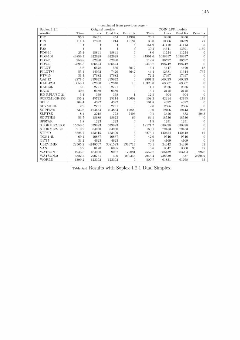
145
– continued from previous page –Soplex 1.2.1 Original models COIN LPP modelsresults Time Iters Dual Its Prim Its Time Iters Dual Its Prim ItsP17 95.2 15451 454 14997 26.1 8850 8850 0P18 111.1 17398 1214 16184 33.0 10306 10279 27P19 f f f f 161.9 41118 41113 5P20 f f f f 30.2 14541 13391 1150PDS-10 25.4 18841 18841 0 8.0 11224 11224 0PDS-100 43859.1 922628 922628 0 47991.6 1058917 1058917 0PDS-20 250.8 52980 52980 0 112.8 36597 36597 0PDS-40 2895.5 186524 186524 0 2443.7 198742 198742 0PILOT 15.6 6578 566 6012 5.4 4447 4429 18PILOT87 55.1 14062 7420 6642 44.4 12381 11644 737PTV15 31.4 17682 17682 0 72.2 17497 17497 0QAP12 2271.5 239642 239642 0 2961.2 360323 360323 0RAIL4284 10058.1 62350 62340 10 10325.0 63067 63067 0RAIL507 13.0 2791 2791 0 11.1 2676 2676 0RAT5 40.6 9489 9489 0 3.1 2118 2118 0RD-RPLUSC-21 5.4 339 338 1 12.5 304 304 0SCFXM1-2R-256 155.8 45722 35114 10608 108.2 42314 42195 119SELF 104.4 4392 4392 0 101.8 4392 4392 0SEYMOUR 2.9 2731 2731 0 2.8 2565 2565 0SGPF5Y6 733.6 124654 104834 19820 10.0 19406 19143 263SLPTSK 8.1 3218 722 2496 9.1 3526 583 2943SOUTH31 53.7 18689 18623 66 64.1 18536 18536 0SP97AR 1.8 1223 1223 0 1.9 1291 1291 0STORMG2 1000 15550.5 679823 679823 0 12171.7 630928 630928 0STORMG2-125 210.2 84930 84930 0 160.1 79153 79153 0STP3D 6726.7 153415 153409 6 5275.1 142454 142442 12T0331-4L 69.1 10837 10837 0 42.0 9546 9546 0T1717 33.2 4623 4623 0 9.9 4169 4169 0ULEVIMIN 22565.2 4748307 3381593 1366714 76.1 24342 24310 32VAN 15.2 8120 8085 35 16.6 8347 8300 47WATSON 1 1943.5 184968 9087 175881 2552.7 386132 383204 2928WATSON 2 6822.5 290751 406 290345 2943.4 238539 537 238002WORLD 1399.2 123302 123302 0 500.7 61831 61768 63
Table A.4: Results with Soplex 1.2.1 Dual Simplex.
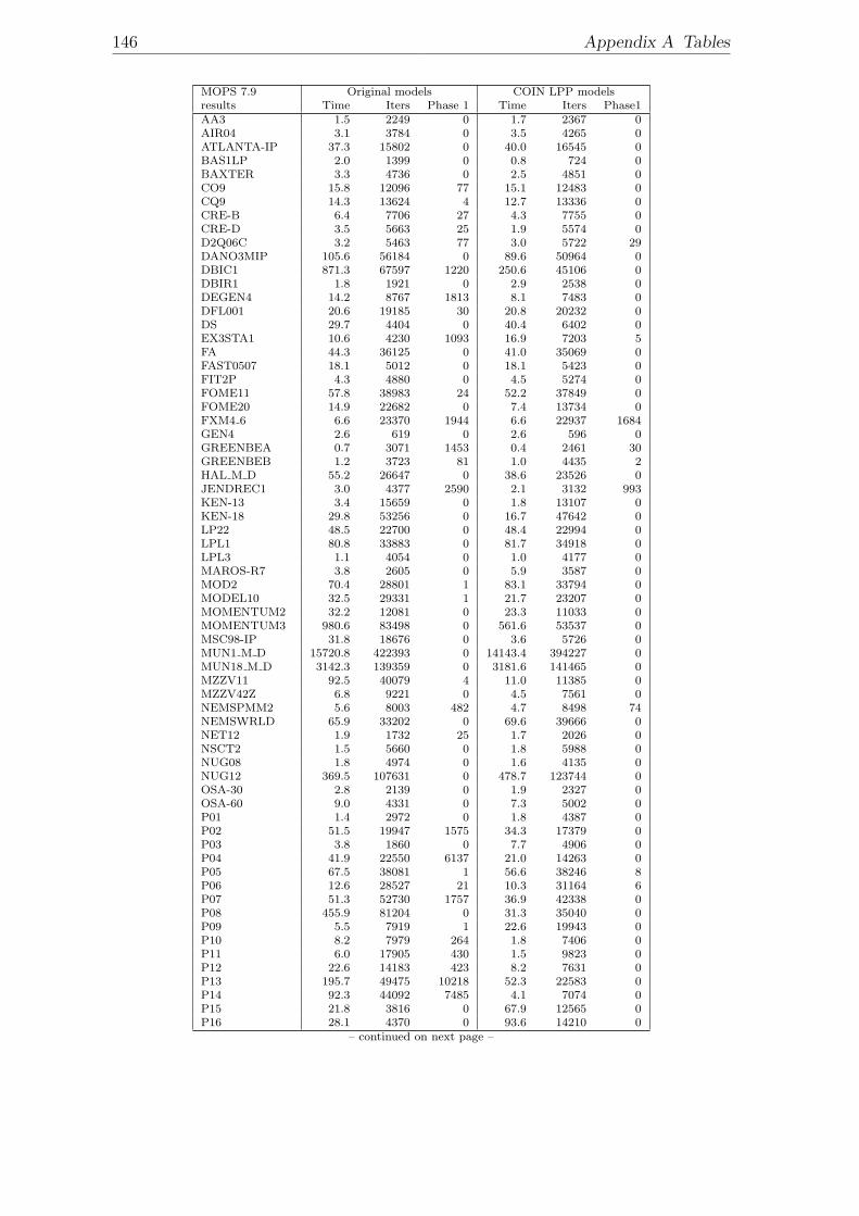
146 Appendix A Tables
MOPS 7.9 Original models COIN LPP modelsresults Time Iters Phase 1 Time Iters Phase1AA3 1.5 2249 0 1.7 2367 0AIR04 3.1 3784 0 3.5 4265 0ATLANTA-IP 37.3 15802 0 40.0 16545 0BAS1LP 2.0 1399 0 0.8 724 0BAXTER 3.3 4736 0 2.5 4851 0CO9 15.8 12096 77 15.1 12483 0CQ9 14.3 13624 4 12.7 13336 0CRE-B 6.4 7706 27 4.3 7755 0CRE-D 3.5 5663 25 1.9 5574 0D2Q06C 3.2 5463 77 3.0 5722 29DANO3MIP 105.6 56184 0 89.6 50964 0DBIC1 871.3 67597 1220 250.6 45106 0DBIR1 1.8 1921 0 2.9 2538 0DEGEN4 14.2 8767 1813 8.1 7483 0DFL001 20.6 19185 30 20.8 20232 0DS 29.7 4404 0 40.4 6402 0EX3STA1 10.6 4230 1093 16.9 7203 5FA 44.3 36125 0 41.0 35069 0FAST0507 18.1 5012 0 18.1 5423 0FIT2P 4.3 4880 0 4.5 5274 0FOME11 57.8 38983 24 52.2 37849 0FOME20 14.9 22682 0 7.4 13734 0FXM4 6 6.6 23370 1944 6.6 22937 1684GEN4 2.6 619 0 2.6 596 0GREENBEA 0.7 3071 1453 0.4 2461 30GREENBEB 1.2 3723 81 1.0 4435 2HAL M D 55.2 26647 0 38.6 23526 0JENDREC1 3.0 4377 2590 2.1 3132 993KEN-13 3.4 15659 0 1.8 13107 0KEN-18 29.8 53256 0 16.7 47642 0LP22 48.5 22700 0 48.4 22994 0LPL1 80.8 33883 0 81.7 34918 0LPL3 1.1 4054 0 1.0 4177 0MAROS-R7 3.8 2605 0 5.9 3587 0MOD2 70.4 28801 1 83.1 33794 0MODEL10 32.5 29331 1 21.7 23207 0MOMENTUM2 32.2 12081 0 23.3 11033 0MOMENTUM3 980.6 83498 0 561.6 53537 0MSC98-IP 31.8 18676 0 3.6 5726 0MUN1 M D 15720.8 422393 0 14143.4 394227 0MUN18 M D 3142.3 139359 0 3181.6 141465 0MZZV11 92.5 40079 4 11.0 11385 0MZZV42Z 6.8 9221 0 4.5 7561 0NEMSPMM2 5.6 8003 482 4.7 8498 74NEMSWRLD 65.9 33202 0 69.6 39666 0NET12 1.9 1732 25 1.7 2026 0NSCT2 1.5 5660 0 1.8 5988 0NUG08 1.8 4974 0 1.6 4135 0NUG12 369.5 107631 0 478.7 123744 0OSA-30 2.8 2139 0 1.9 2327 0OSA-60 9.0 4331 0 7.3 5002 0P01 1.4 2972 0 1.8 4387 0P02 51.5 19947 1575 34.3 17379 0P03 3.8 1860 0 7.7 4906 0P04 41.9 22550 6137 21.0 14263 0P05 67.5 38081 1 56.6 38246 8P06 12.6 28527 21 10.3 31164 6P07 51.3 52730 1757 36.9 42338 0P08 455.9 81204 0 31.3 35040 0P09 5.5 7919 1 22.6 19943 0P10 8.2 7979 264 1.8 7406 0P11 6.0 17905 430 1.5 9823 0P12 22.6 14183 423 8.2 7631 0P13 195.7 49475 10218 52.3 22583 0P14 92.3 44092 7485 4.1 7074 0P15 21.8 3816 0 67.9 12565 0P16 28.1 4370 0 93.6 14210 0
– continued on next page –
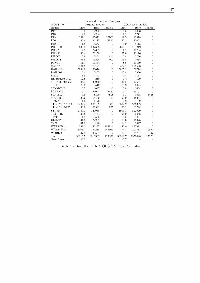
147
– continued from previous page –MOPS 7.9 Original models COIN LPP modelsresults Time Iters Phase 1 Time Iters Phase1P17 3.9 2265 0 6.5 5033 0P18 4.0 2284 0 7.1 5271 0P19 251.4 65871 12706 19.5 10918 0P20 45.6 26185 5855 30.2 22062 0PDS-10 1.8 6833 0 1.0 5118 0PDS-100 636.9 237628 0 319.1 151212 0PDS-20 14.9 22682 0 7.1 13734 0PDS-40 86.4 70158 0 37.8 42116 0PILOT 3.8 3493 116 3.8 3796 0PILOT87 31.5 11265 102 16.5 7035 0PTV15 11.7 13564 0 8.8 13160 0QAP12 281.5 80121 0 462.1 125538 0RAIL4284 5944.9 56076 0 5865.1 56714 0RAIL507 16.4 3405 0 12.4 2836 0RAT5 1.9 2142 0 1.8 2137 0RD-RPLUSC-21 17.8 210 1 0.4 179 0SCFXM1-2R-256 28.3 35062 0 36.5 37667 0SELF 183.3 8519 0 125.2 6024 0SEYMOUR 3.5 4097 15 2.8 3664 0SGPF5Y6 17.7 44023 12132 2.7 25767 0SLPTSK 9.6 8300 7818 3.1 3868 3438SOUTH31 30.2 18402 19 29.0 18264 0SP97AR 1.3 1170 0 1.2 1159 0STORMG2 1000 3464.4 506109 1000 3894.7 556389 0STORMG2-125 38.9 62391 125 36.2 63794 0STP3D 2769.1 149935 0 1993.3 122929 0T0331-4L 23.8 5754 0 24.0 6488 0T1717 11.5 3585 0 8.5 4401 0ULEVIMIN 41.5 22282 1 18.0 15925 0VAN 47.8 14198 0 14.1 8827 0WATSON 1 238.2 145297 104811 140.9 137312 0WATSON 2 1301.7 264235 249365 174.2 201317 10954WORLD 97.5 33584 2 111.4 38704 97Sum 38816.5 3816302 433351 33312.7 3376048 17320Geo. Mean 23.0 – – 15.7 – –
Table A.5: Results with MOPS 7.9 Dual Simplex.
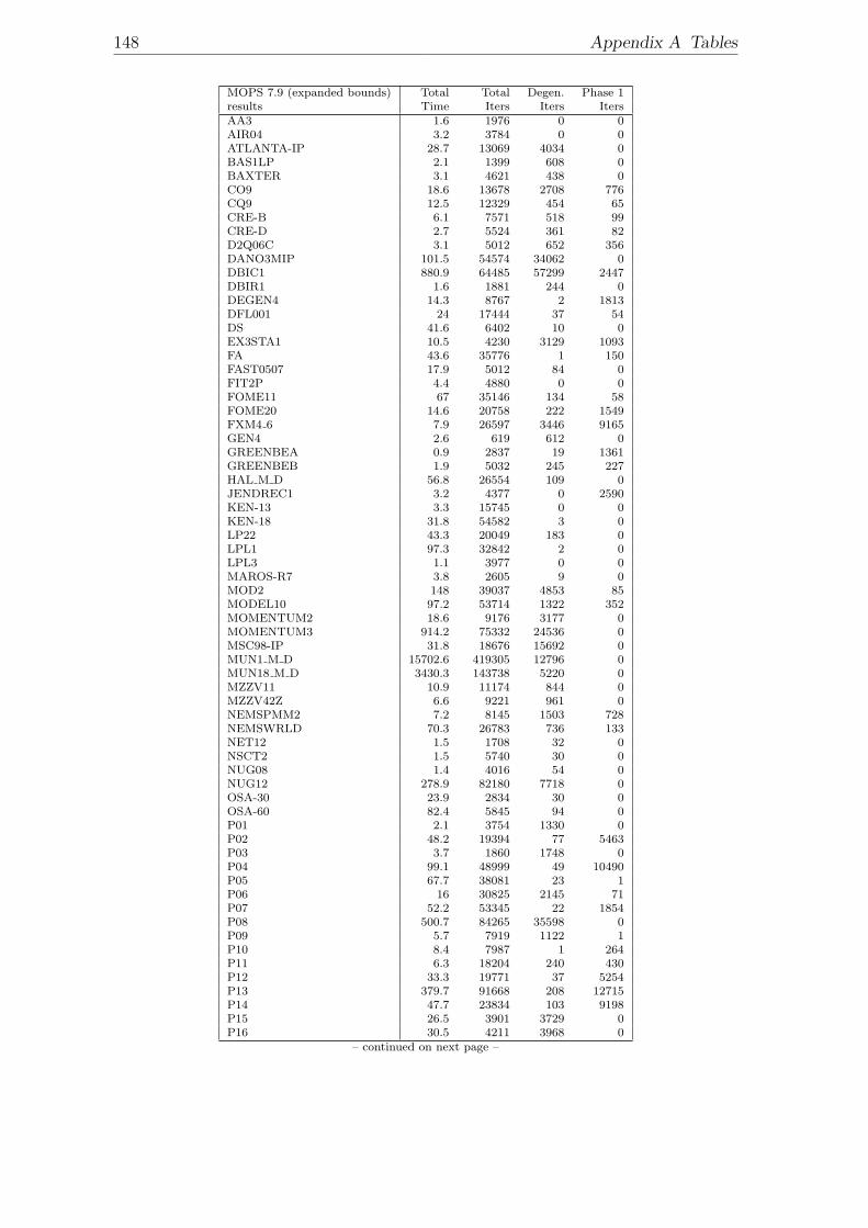
148 Appendix A Tables
MOPS 7.9 (expanded bounds) Total Total Degen. Phase 1results Time Iters Iters ItersAA3 1.6 1976 0 0AIR04 3.2 3784 0 0ATLANTA-IP 28.7 13069 4034 0BAS1LP 2.1 1399 608 0BAXTER 3.1 4621 438 0CO9 18.6 13678 2708 776CQ9 12.5 12329 454 65CRE-B 6.1 7571 518 99CRE-D 2.7 5524 361 82D2Q06C 3.1 5012 652 356DANO3MIP 101.5 54574 34062 0DBIC1 880.9 64485 57299 2447DBIR1 1.6 1881 244 0DEGEN4 14.3 8767 2 1813DFL001 24 17444 37 54DS 41.6 6402 10 0EX3STA1 10.5 4230 3129 1093FA 43.6 35776 1 150FAST0507 17.9 5012 84 0FIT2P 4.4 4880 0 0FOME11 67 35146 134 58FOME20 14.6 20758 222 1549FXM4 6 7.9 26597 3446 9165GEN4 2.6 619 612 0GREENBEA 0.9 2837 19 1361GREENBEB 1.9 5032 245 227HAL M D 56.8 26554 109 0JENDREC1 3.2 4377 0 2590KEN-13 3.3 15745 0 0KEN-18 31.8 54582 3 0LP22 43.3 20049 183 0LPL1 97.3 32842 2 0LPL3 1.1 3977 0 0MAROS-R7 3.8 2605 9 0MOD2 148 39037 4853 85MODEL10 97.2 53714 1322 352MOMENTUM2 18.6 9176 3177 0MOMENTUM3 914.2 75332 24536 0MSC98-IP 31.8 18676 15692 0MUN1 M D 15702.6 419305 12796 0MUN18 M D 3430.3 143738 5220 0MZZV11 10.9 11174 844 0MZZV42Z 6.6 9221 961 0NEMSPMM2 7.2 8145 1503 728NEMSWRLD 70.3 26783 736 133NET12 1.5 1708 32 0NSCT2 1.5 5740 30 0NUG08 1.4 4016 54 0NUG12 278.9 82180 7718 0OSA-30 23.9 2834 30 0OSA-60 82.4 5845 94 0P01 2.1 3754 1330 0P02 48.2 19394 77 5463P03 3.7 1860 1748 0P04 99.1 48999 49 10490P05 67.7 38081 23 1P06 16 30825 2145 71P07 52.2 53345 22 1854P08 500.7 84265 35598 0P09 5.7 7919 1122 1P10 8.4 7987 1 264P11 6.3 18204 240 430P12 33.3 19771 37 5254P13 379.7 91668 208 12715P14 47.7 23834 103 9198P15 26.5 3901 3729 0P16 30.5 4211 3968 0
– continued on next page –
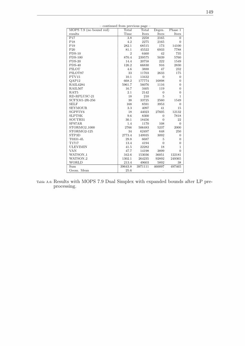
149
– continued from previous page –MOPS 7.9 (no bound red) Total Total Degen. Phase 1results Time Iters Iters ItersP17 3.8 2258 2165 0P18 4.2 2275 2165 0P19 282.1 68515 173 14100P20 81.1 45522 6933 7788PDS-10 2 6460 42 735PDS-100 870.4 239575 5039 5760PDS-20 14.4 20758 222 1549PDS-40 126.2 66830 916 2830PILOT 4.6 3888 47 232PILOT87 33 11703 2633 175PTV15 10.1 13432 0 0QAP12 668.2 177774 16898 0RAIL4284 5961.7 56076 1116 0RAIL507 16.7 3405 119 0RAT5 2.1 2142 0 0RD-RPLUSC-21 18 210 5 1SCFXM1-2R-256 38 33725 2560 1549SELF 168 8591 3953 0SEYMOUR 3.3 4097 41 15SGPF5Y6 18 44023 27605 12132SLPTSK 9.6 8300 0 7818SOUTH31 30.1 18456 0 22SP97AR 1.4 1170 108 0STORMG2 1000 2766 506483 5237 2000STORMG2-125 34 62497 648 250STP3D 2773.4 149935 3092 0T0331-4L 29.8 6687 5 0T1717 13.4 4194 0 0ULEVIMIN 41.5 22282 18 1VAN 47.7 14198 3899 0WATSON 1 342.6 153036 36051 122181WATSON 2 1302.1 264235 92892 249365WORLD 213.4 49603 5892 38Sum 39643.8 3971111 460097 497465Geom. Mean 25.6 – – –
Table A.6: Results with MOPS 7.9 Dual Simplex with expanded bounds after LP pre-processing.
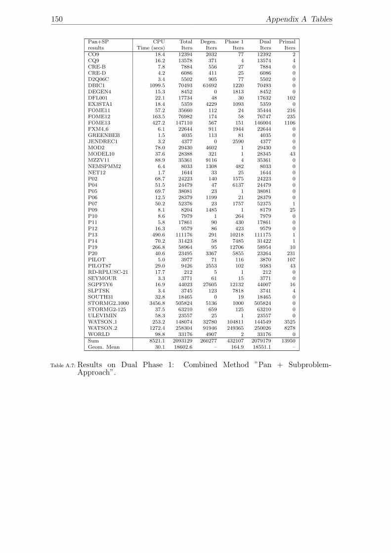
150 Appendix A Tables
Pan+SP CPU Total Degen. Phase 1 Dual Primalresults Time (secs) Iters Iters Iters Iters ItersCO9 18.4 12394 2032 77 12392 2CQ9 16.2 13578 371 4 13574 4CRE-B 7.8 7884 556 27 7884 0CRE-D 4.2 6086 411 25 6086 0D2Q06C 3.4 5502 905 77 5502 0DBIC1 1099.5 70493 61692 1220 70493 0DEGEN4 15.3 8452 0 1813 8452 0DFL001 22.1 17734 48 30 17632 102EX3STA1 18.4 5359 4229 1093 5359 0FOME11 57.2 35660 112 24 35444 216FOME12 163.5 76982 174 58 76747 235FOME13 427.2 147110 567 151 146004 1106FXM4 6 6.1 22644 911 1944 22644 0GREENBEB 1.5 4035 113 81 4035 0JENDREC1 3.2 4377 0 2590 4377 0MOD2 78.0 29430 4602 1 29430 0MODEL10 37.6 28388 321 1 28345 43MZZV11 88.9 35361 9116 4 35361 0NEMSPMM2 6.4 8033 1308 482 8033 0NET12 1.7 1644 33 25 1644 0P02 68.7 24223 140 1575 24223 0P04 51.5 24479 47 6137 24479 0P05 69.7 38081 23 1 38081 0P06 12.5 28379 1199 21 28379 0P07 50.2 52376 23 1757 52375 1P09 8.1 8204 1485 1 8179 25P10 8.6 7979 1 264 7979 0P11 5.8 17861 90 430 17861 0P12 16.3 9579 86 423 9579 0P13 490.6 111176 291 10218 111175 1P14 70.2 31423 58 7485 31422 1P19 266.8 58964 95 12706 58954 10P20 40.6 23495 3367 5855 23264 231PILOT 5.0 3977 71 116 3870 107PILOT87 29.0 9426 2553 102 9383 43RD-RPLUSC-21 17.7 212 5 1 212 0SEYMOUR 3.3 3771 61 15 3771 0SGPF5Y6 16.9 44023 27605 12132 44007 16SLPTSK 3.4 3745 123 7818 3741 4SOUTH31 32.8 18465 0 19 18465 0STORMG2 1000 3456.8 505824 5136 1000 505824 0STORMG2-125 37.5 63210 659 125 63210 0ULEVIMIN 58.3 23557 25 1 23557 0WATSON 1 253.2 148074 32780 104811 144549 3525WATSON 2 1272.4 258304 91946 249365 250026 8278WORLD 98.8 33176 4907 2 33176 0Sum 8521.1 2093129 260277 432107 2079179 13950Geom. Mean 30.1 18602.6 – 164.9 18551.1 –
Table A.7: Results on Dual Phase 1: Combined Method ”Pan + Subproblem-Approach”.
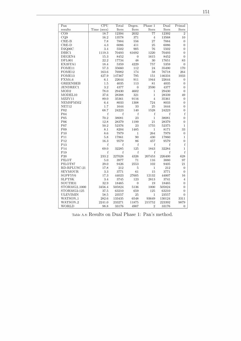
151
Pan CPU Total Degen. Phase 1 Dual Primalresults Time (secs) Iters Iters Iters Iters ItersCO9 18.7 12394 2032 77 12392 2CQ9 16.2 13578 371 4 13568 10CRE-B 7.8 7884 556 27 7884 0CRE-D 4.3 6086 411 25 6086 0D2Q06C 3.4 5502 905 76 5502 0DBIC1 1119.3 70493 61692 1220 70493 0DEGEN4 15.3 8452 0 1615 8452 0DFL001 22.2 17734 48 30 17651 83EX3STA1 18.4 5359 4229 757 5359 0FOME11 57.3 35660 112 24 35490 170FOME12 163.6 76982 174 58 76718 264FOME13 427.9 147367 795 151 146334 1033FXM4 6 6.1 22644 911 1944 22644 0GREENBEB 1.5 4035 113 81 4035 0JENDREC1 3.2 4377 0 2590 4377 0MOD2 78.0 29430 4602 1 29430 0MODEL10 37.6 28388 321 1 28339 49MZZV11 89.0 35361 9116 4 35361 0NEMSPMM2 6.4 8033 1308 724 8033 0NET12 1.7 1644 33 25 1644 0P02 68.7 24223 140 1528 24223 0P04 f f f f f fP05 70.2 38081 23 1 38081 0P06 12.8 28379 1199 21 28379 0P07 50.2 52376 23 1755 52375 1P09 8.1 8204 1485 1 8171 33P10 8.6 7979 1 264 7979 0P11 5.8 17861 90 430 17860 1P12 16.3 9579 86 457 9579 0P13 f f f f f fP14 69.0 32285 125 1843 32284 1P19 f f f f f fP20 233.2 227028 4326 207453 226400 628PILOT 5.0 3977 71 116 3880 97PILOT87 29.0 9426 2553 102 9405 21RD-RPLUSC-21 17.8 212 5 1 212 0SEYMOUR 3.3 3771 61 15 3771 0SGPF5Y6 17.3 44023 27605 12132 44007 16SLPTSK 3.4 3745 123 2813 3741 4SOUTH31 32.9 18465 0 19 18465 0STORMG2 1000 3456.4 505824 5136 1000 505824 0STORMG2-125 37.5 63210 659 125 63210 0ULEVIMIN 58.5 23557 25 1 23557 0WATSON 1 282.6 133435 6548 93649 130124 3311WATSON 2 2241.0 233271 11875 215752 223392 9879WORLD 98.8 33176 4907 2 33176 0
Table A.8: Results on Dual Phase 1: Pan’s method.
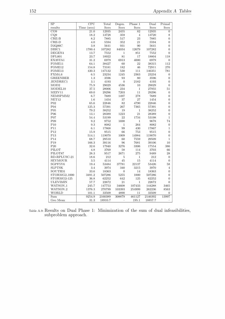
152 Appendix A Tables
SP CPU Total Degen. Phase 1 Dual Primalresults Time (secs) Iters Iters Iters Iters ItersCO9 21.0 12935 2455 82 12935 0CQ9 18.2 13728 359 4 13720 8CRE-B 8.2 7885 517 23 7885 0CRE-D 4.0 5594 352 21 5594 0D2Q06C 3.8 5641 931 90 5641 0DBIC1 1700.4 107282 84034 12679 107282 0DEGEN4 13.7 7552 1 851 7552 0DFL001 23.7 18922 81 17 18804 118EX3STA1 31.2 6979 6913 4000 6979 0FOME11 64.1 38427 60 22 38315 112FOME12 154.8 73181 182 46 72911 270FOME13 430.3 147132 530 111 146351 781FXM4 6 6.5 23234 1245 2363 23234 0GREENBEB 1.3 3596 93 80 3596 0JENDREC1 3.1 4193 0 2182 4193 0MOD2 75.9 29029 4536 10 29029 0MODEL10 37.5 28006 234 1 27955 51MZZV11 69.0 29296 7203 11 29296 0NEMSPMM2 6.7 7689 1497 278 7689 0NET12 1.6 1454 37 27 1454 0P02 65.6 22846 82 4790 22846 0P04 125.3 57391 267 7365 57391 0P05 79.2 38252 19 1 38252 0P06 13.1 28389 1223 21 28389 0P07 54.4 53199 22 1734 53198 1P09 9.2 9752 1690 1 9678 74P10 9.3 8082 1 264 8082 0P11 6.1 17868 99 430 17867 1P12 15.9 9515 66 753 9515 0P13 514.1 119070 1009 14984 119070 0P14 68.7 29510 60 7559 29509 1P19 166.3 39116 96 7681 39106 10P20 32.6 17940 3276 3306 17554 386PILOT 4.8 3769 58 114 3703 66PILOT87 28.3 9517 2671 275 9489 28RD-RPLUSC-21 18.6 212 5 1 212 0SEYMOUR 3.5 4114 45 15 4114 0SGPF5Y6 19.4 53484 37781 22137 53426 58SLPTSK 3.4 3974 340 3215 3970 4SOUTH31 33.6 18363 0 14 18363 0STORMG2 1000 3491.2 507286 5255 1000 507286 0STORMG2-125 36.8 62252 642 125 62252 0ULEVIMIN 57.7 22672 21 1 22672 0WATSON 1 245.7 147753 34608 107433 144288 3465WATSON 2 1376.3 270799 103393 254999 262236 8563WORLD 101.1 33509 4890 11 33509 0Sum 9254.9 2160389 308879 461127 2146392 13997Geo Mean 31.3 18910.7 – 195.1 18857.7 –
Table A.9: Results on Dual Phase 1: Minimization of the sum of dual infeasibilities,subproblem approach.
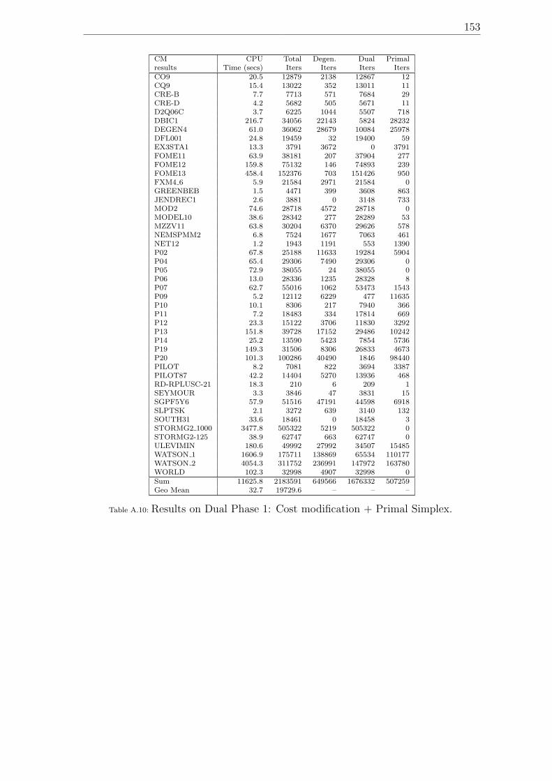
153
CM CPU Total Degen. Dual Primalresults Time (secs) Iters Iters Iters ItersCO9 20.5 12879 2138 12867 12CQ9 15.4 13022 352 13011 11CRE-B 7.7 7713 571 7684 29CRE-D 4.2 5682 505 5671 11D2Q06C 3.7 6225 1044 5507 718DBIC1 216.7 34056 22143 5824 28232DEGEN4 61.0 36062 28679 10084 25978DFL001 24.8 19459 32 19400 59EX3STA1 13.3 3791 3672 0 3791FOME11 63.9 38181 207 37904 277FOME12 159.8 75132 146 74893 239FOME13 458.4 152376 703 151426 950FXM4 6 5.9 21584 2971 21584 0GREENBEB 1.5 4471 399 3608 863JENDREC1 2.6 3881 0 3148 733MOD2 74.6 28718 4572 28718 0MODEL10 38.6 28342 277 28289 53MZZV11 63.8 30204 6370 29626 578NEMSPMM2 6.8 7524 1677 7063 461NET12 1.2 1943 1191 553 1390P02 67.8 25188 11633 19284 5904P04 65.4 29306 7490 29306 0P05 72.9 38055 24 38055 0P06 13.0 28336 1235 28328 8P07 62.7 55016 1062 53473 1543P09 5.2 12112 6229 477 11635P10 10.1 8306 217 7940 366P11 7.2 18483 334 17814 669P12 23.3 15122 3706 11830 3292P13 151.8 39728 17152 29486 10242P14 25.2 13590 5423 7854 5736P19 149.3 31506 8306 26833 4673P20 101.3 100286 40490 1846 98440PILOT 8.2 7081 822 3694 3387PILOT87 42.2 14404 5270 13936 468RD-RPLUSC-21 18.3 210 6 209 1SEYMOUR 3.3 3846 47 3831 15SGPF5Y6 57.9 51516 47191 44598 6918SLPTSK 2.1 3272 639 3140 132SOUTH31 33.6 18461 0 18458 3STORMG2 1000 3477.8 505322 5219 505322 0STORMG2-125 38.9 62747 663 62747 0ULEVIMIN 180.6 49992 27992 34507 15485WATSON 1 1606.9 175711 138869 65534 110177WATSON 2 4054.3 311752 236991 147972 163780WORLD 102.3 32998 4907 32998 0Sum 11625.8 2183591 649566 1676332 507259Geo Mean 32.7 19729.6 – – –
Table A.10: Results on Dual Phase 1: Cost modification + Primal Simplex.
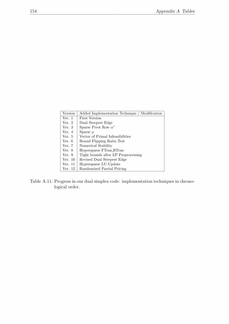
154 Appendix A Tables
Version Added Implementation Technique / ModificationVer. 1 First VersionVer. 2 Dual Steepest EdgeVer. 3 Sparse Pivot Row αr
Ver. 4 Sparse ρVer. 5 Vector of Primal InfeasibilitiesVer. 6 Bound Flipping Ratio TestVer. 7 Numerical StabilityVer. 8 Hypersparse FTran,BTranVer. 9 Tight bounds after LP PreprocessingVer. 10 Revised Dual Steepest EdgeVer. 11 Hypersparse LU-UpdateVer. 12 Randomized Partial Pricing
Table A.11: Progress in our dual simplex code: implementation techniques in chrono-logical order.
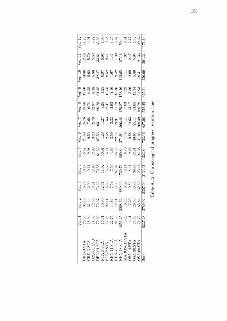
155
Ver
.1
Ver
.2
Ver
.3
Ver
.4
Ver
.5
Ver
.6
Ver
.7
Ver
.8
Ver
.9
Ver
.10
Ver
.11
Ver
.12
CR
E-B
.STA
26.5
635
.78
16.2
019
.17
18.4
721
.59
15.7
618
.56
13.8
014
.86
12.4
811
.78
CR
E-D
.STA
18.9
431
.44
12.0
09.
119.
089.
507.
686.
786.
555.
625.
704.
91D
2Q06
C.S
TA
11.0
312
.50
12.8
112
.98
12.9
213
.20
12.7
812
.97
8.38
5.80
5.53
5.77
DFL00
1.ST
A72
.69
72.2
773
.69
70.5
861
.53
67.5
363
.11
60.2
064
.58
32.4
733
.61
35.2
6FIT
2D.S
TA
10.3
110
.80
12.3
111
.02
10.9
71.
281.
271.
251.
250.
970.
971.
00FIT
2P.S
TA
17.2
522
.11
15.3
916
.33
15.1
112
.48
11.5
312
.47
12.5
89.
529.
419.
38K
EN
-11.
STA
22.7
514
.86
7.53
7.53
4.66
3.59
3.32
2.93
2.10
1.67
1.41
1.25
KE
N-1
3.ST
A19
4.53
112.
4175
.33
87.9
446
.14
22.7
419
.91
11.7
913
.36
9.42
7.39
6.27
KE
N-1
8.ST
A48
56.2
522
68.6
218
89.3
917
20.7
686
0.84
371.
9130
6.48
159.
8715
8.46
112.
0587
.16
59.4
4M
AR
OS-
R7.
STA
5.28
6.48
6.09
6.11
6.70
7.78
7.11
7.03
7.22
7.11
7.92
6.81
OSA
-14.
STA
4.41
7.25
9.80
8.41
9.23
10.5
814
.63
13.1
73.
562.
092.
472.
17O
SA-3
0.ST
A15
.56
29.5
643
.86
39.8
943
.81
49.9
555
.11
54.6
511
.34
5.80
5.95
6.42
OSA
-60.
STA
71.7
216
5.84
132.
6912
3.48
124.
3814
1.03
168.
3916
6.78
21.9
319
.31
21.3
320
.67
Sum
5327
.28
2789
.92
2307
.09
2133
.31
1223
.84
733.
1668
7.08
528.
4532
5.11
226.
6920
1.33
171.
13
Tab
leA
.12:
Chro
nol
ogic
alpro
gres
s:so
luti
onti
me.
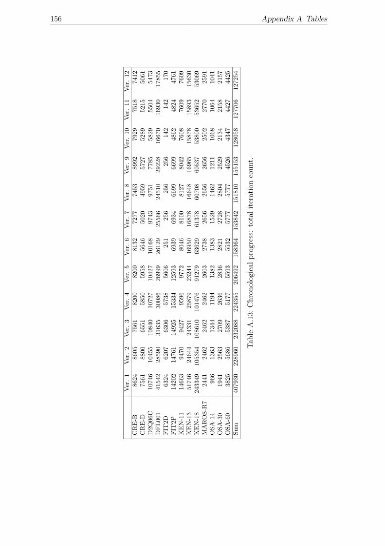
156 Appendix A Tables
Ver
.1
Ver
.2
Ver
.3
Ver
.4
Ver
.5
Ver
.6
Ver
.7
Ver
.8
Ver
.9
Ver
.10
Ver
.11
Ver
.12
CR
E-B
8624
8605
7561
8200
8200
8132
7277
7453
8992
7929
7518
7412
CR
E-D
7561
8800
6551
5850
5958
5646
5020
4959
5727
5289
5215
5061
D2Q
06C
1074
610
455
1084
010
727
1042
710
168
9743
9751
7785
5829
5504
5473
DFL00
141
542
2859
031
635
3008
626
999
2612
925
566
2451
029
228
1667
016
930
1785
5FIT
2D63
2462
0763
0657
3856
0625
125
625
625
614
214
217
0FIT
2P14
202
1476
114
925
1533
412
593
6939
6934
6699
6699
4862
4824
4761
KE
N-1
114
663
9470
9427
9596
9772
8046
8100
8127
8042
7608
7609
7609
KE
N-1
351
746
2464
424
331
2587
923
244
1695
016
878
1664
816
965
1587
815
893
1563
0K
EN
-18
2433
4910
5354
1086
1010
1476
9127
963
629
6137
860
708
6053
753
800
5365
253
069
MA
RO
S-R
724
4124
6224
6224
6226
0327
3826
5626
5626
5625
0227
7025
91O
SA-1
496
613
6313
4411
9413
8213
8315
2914
6212
1110
6810
6410
41O
SA-3
019
4125
6327
0926
3628
3628
2127
2828
0425
2921
3421
5821
57O
SA-6
038
2556
8653
8751
7755
9355
3257
7757
7745
2643
4744
2744
25Su
m40
7930
2289
6023
2088
2243
5520
6492
1583
6415
3842
1518
1015
5153
1280
5812
7706
1272
54
Tab
leA
.13:
Chro
nol
ogic
alpro
gres
s:to
talit
erat
ion
count.