1

June 2011

The Determinants of Attitudes towards Strategic

Default on Mortgages∗

Luigi Guiso European University Institute, EIEF, & CEPR

Paola Sapienza Northwestern University, NBER, & CEPR

Luigi Zingales University of Chicago, NBER, & CEPR

Abstract We use survey data to measure households’ propensity to default on mortgages even if they can afford to pay them (strategic default) when the value of the mortgage exceeds the value of the house. The willingness to default increases both in the absolute and in the relative size of the home-equity shortfall. Our evidence suggests that this willingness is affected both by pecuniary and non-pecuniary factors, such as views about fairness and morality. We also find that exposure to other people who strategically defaulted increases the propensity to default strategically because it conveys information about the probability of being sued.

∗An earlier version of this paper circulated with the title “Moral and Social Constraints to Strategic Default on Mortgages.” We would like to thank the University of Chicago Booth School of Business and Kellogg School of Management for financial support in establishing and maintaining the Chicago Booth Kellogg School Financial Trust Index. Luigi Guiso is grateful to PEGGED for financial support. We thank Campbell Harvey (editor), Amir Sufi, two anonymous referee and seminar participants at the University of Chicago and New York University for very useful suggestions, Gabriella Santangelo and Filippo Mezzanotti for excellent research assistantship, and Peggy Eppink for editorial help. We also thank Amit Seru for providing us with a time series of actual strategic default within his sample.

2

In 2009, for the first time since the Great Depression, millions of American households found

themselves with a mortgage that exceeded the value of their home. According to First American

CoreLogic, more than 15.2 million U.S. mortgages, or 32.2 percent of all mortgaged properties,

were in a negative equity position as of June 30, 2009, while in some states (such as Arizona and

Nevada) this number exceeded 50%.1 Importantly, the difference between the value of the house

and that of the mortgage is often very large. For example, in 2009 the median owner’s equity for

those who bought a house in the Salinas, CA metropolitan statistical area (MSA) in 2006 was

$214,305.2 Given the magnitude of this phenomenon, it is important to address the question of

whether homeowners with such a large negative equity value will choose to walk away from their

houses even if they can afford to pay their mortgages, an action known as a strategic default.

Unfortunately, we know very little about the importance and the determinants of strategic

default on mortgages.3 In an influential paper, Foote et al. (2008) show that during the 1990–91

recession in Massachusetts very few people (6.4%) chose to walk away from their houses when

their home equity was negative. Yet, the 1990s behavior of Massachusetts residents may not be

predictive of the national behavior during the 2007–09 recession, since conditions were different

and there are important nonlinearities. Hence, in assessing the risk of strategic default, what matters

is not the average decline in home prices, but the decline in the worst-hit areas.

The main problem in studying strategic defaults is that this is de facto an unobservable

event. While we do observe defaults, we cannot observe whether a default is strategic. Strategic

defaulters have incentives to disguise themselves as people who cannot afford to pay so they are

difficult to identify in the data.

Given this constraint, one way to assess the likelihood of a strategic default is to estimate a

structural model of default that includes both cash flow considerations and negative equity

considerations. One can then use the estimated parameters to simulate a shock to home equity alone

and compute the predicted effect. This strategy has been followed by Bajari et al (2008), who

estimate that ceteris paribus a 20% decline in home prices would lead to a 15% increase in the

probability that a borrower would default.

An alternative way, which we follow in this paper, is to resort to survey data. To this end,

we study a new quarterly survey of a representative sample of U.S. households. We use the waves

1 http://www.corelogic.com/About-Us/ResearchTrends/Negative-Equity-Report.aspx. A study by Deutsche Bank estimated that the 26% of the homeowners had negative equity in the first quarter of 2009 and projected this number to be 48% for the first quarter of 2011. 2 http://www.zillow.com/reports/RealEstateMarketReports.htm. 3 There exists a parallel literature on strategic default for personal loans. While households file for bankruptcy less often than their financial incentives suggest (White, 1998), they are more likely to file when their financial benefit from filing is higher (Fay et al, 2002).

3

from December 2008 (the first) to September 2010 for two purposes: to identify the percentage of

current defaults that is strategic and to study the determinants of homeowners’ attitudes towards

strategic default.

To identify the proportion of strategic default, we use two questions. One asks “How many

people do you know who have defaulted on their house mortgage?” Those who know at least one,

are also asked “Of the people you know who have defaulted on their mortgage, how many do you

think walked away even if they could afford to pay the monthly mortgage?” By taking a ratio of the

two, we obtain an estimate of the percentage of actual defaults that are considered “strategic” by the

defaulters’ acquaintances.

We find that this proportion is large and rising. In March 2009, 26.4% of defaults appear

strategic, in September 2010 that number rose to 35.1%. As we discuss in the paper, both the level

and the trend we have identified are corroborated by subsequent studies using borrower level data

(Experian and Oliver Wyman (2009), Tiruppatur et al. (2010), and Goodman (2009)).

Given the importance of strategic default, we study the drivers behind homeowners’

attitudes towards strategic default. As such, we use the answers to the question “If the value of your

mortgage exceeded the value of your house by 50K [100K/150K] would you walk away from your

house (that is, default on your mortgage) even if you could afford to pay your monthly mortgage?”

By using these answers we can infer the shape of the function relating the overall cost of

defaulting to wealth. The overall cost appears to be increasing in wealth, but at a decreasing rate.

Doubling the ratio of home equity shortfall to house value increases the frequency of homeowners

who express a willingness to default by 10.4 percentage points when starting from a house value of

200–400K (Table 1B), but only by 2.7 percentage points if we halve the value of the house. Then,

we correlate the declared willingness to walk away when the equity shortfall is equal to

$50K/$100K with various proxies for the typical economic drivers of this decision: cost of

relocation (number of children, number of years in the current location), the risk of losing other

assets (whether the respondent is in a nonrecourse state), the stability of the financial position

(income and probability of becoming unemployed).

We find that the cost of defaulting strategically is driven both by pecuniary and non-

pecuniary components, such as views about fairness and morality. Not surprisingly, the biggest

determinants are the value of the equity shortfall as a percentage of the house value and whether the

house was bought more than 5 years ago—a measure of the attachment to (and thus the cost of

leaving) the current location. Ceteris paribus, a one standard deviation increase in the relative size

of this hypothetical equity shortfall increases the probability of strategic default by 25%, but a

person who has bought his house more than five years ago is 28% less likely to default.

4

We also find that ceteris paribus blacks, Hispanics, and older people are more willing to

strategically default, while women are less likely. The fear of becoming unemployed also plays a

role. If a person becomes unemployed, it is likely they will be forced to default in the future.

Anticipating this possibility reduces the benefit of not defaulting strategically today. A one standard

deviation increase in the perceived probability of becoming unemployed increases the probability of

strategic default by 13% of sample mean.

Surprisingly, whether or not the fact that a state requires mortgages to be non-recourse (i.e.,

the lender cannot go after his/her wealth outside of the house) does not seem to affect the

willingness to default strategically. One possible reason is that most people do not know the legal

status of mortgages in their state, the other is that most people do not have any assets outside their

house and thus the difference between recourse and non-recourse is moot. To test the first

hypothesis, starting with the 5th wave of the survey, we asked people for their subjective estimate of

the probability a bank will go after a defaulted borrower. On average this subjective probability is

53.4%, and does not differ between recourse and non-recourse states.

Then, we consider moral and social determinants of the attitudes towards strategic default.

Eighty-two percent of the people think it is morally wrong to engage in a strategic default.

Everything else being equal, people who think that it is immoral to default strategically are 9.9

percentage points less likely to declare strategic default. Even if the morality question is asked after

the willingness to default strategically question, this correlation could be spurious, and may be the

result of the respondent’s desire to be consistent across responses (i.e., to answer that it is not

immoral to default after responding that they will default). Since, waves 3 to 8 of the survey

randomizes the order of the morality and default questions, we use this randomization to correct the

estimate for the potential spurious correlation in the responses. While smaller, we find that the

effect of morality on the probability of default persists even after the correction.

Consistent with the literature on personal bankruptcy (Fay et al. (2002) and Gross and

Souleles (2002)), the decision to default strategically might be driven by other emotional

considerations. People have been shown to be more likely to inflict a loss on others when they have

suffered a loss themselves, especially if they consider their loss to be unfair (Fowler et al, 2005).

For this reason, we regress the willingness to default strategically on some measures of anger and

trust. We find that people who are angrier about the current economic situation are more willing to

express their willingness to default, as are people who trust banks less. Similarly, people who want

to regulate executive compensations and the financial sectors are more likely to declare their

willingness to walk away.

5

Finally, we find that people who know somebody who defaulted strategically are more

likely to declare their intention to do so. This effect is present even if we control for the number of

foreclosures in the area and for whether the respondent knows somebody who defaulted non-

strategically. This effect could be the result of a social contagion, of some learning about the cost of

defaulting strategically or the spurious effect of clustering: people with lower moral standards live

nearby and know each other. We do not find any evidence for the clustering effect. Ceteris paribus,

knowing somebody who defaulted does not affect the moral attitude toward defaulting. By contrast,

there is evidence consistent with the learning hypothesis: Knowing somebody who strategically

defaulted reduces the perceived probability that a bank would go after a borrower who defaults.

On average, we find that homeowners’ declared willingness to default per given home

equity shortfall is roughly constant during the period covered by our data (December 2008–

September 2010). This stability is the result of two opposite effects. On the one hand, there is a

decreased level of anger, which reduces the willingness to default; on the other hand, learning about

the cost of defaulting, over time, increases the willingness to default. Given the stability in the

willingness to default per given size of the shortfall, the most likely cause of the increased

proportion of strategic default between March 09 and September 09 is the decline in house prices.

While aggregate house prices continued to slide during the entire period, the declined in the areas

where more homeowners have negative equity are concentrated up to the mid of 2009, as shown in

Figure 11. As of the second quarter of 2009 house prices stabilized in the areas where they had

declined the most in the previous period, but they continued to slide in the areas where they had not

dropped much before. As a result, the percentage of households with negative equity, which

increased dramatically from the second quarter 2008 to the second quarter 2009, stabilized, thereby

stabilizing the frequency of strategic defaults after September 2009.

The rest of the paper proceeds as follows. Section 1 introduces the theoretical framework.

Section 2 describes the new survey data used in the paper. Section 3 presents some evidence on the

importance of strategic default. Section 4 presents the results on the determinants of strategic

default. Section 5 discusses the possible reasons of the increase of strategic defaults over time.

Conclusions follow.

1. The Theoretical Framework

The narrowest economic framework would hold that in non-recourse states a household will default

whenever the value of the mortgage exceeds the value of the house (e.g., see White, 2009). While

negative equity is a necessary condition for strategic default, it is not sufficient. Even in non-

recourse states, there are frictions that make defaulting less appealing.

6

Let’s start by considering a borrower who at time t owns a house worth Ht and faces a

mortgage-balloon payment equal to Dt. From a purely financial point of view the borrower will not

default as long as Ht > Dt. In the decision whether to default strategically, however, there are

considerations others than the financial gain or loss from defaulting. By non-defaulting, for

example, a borrower enjoys non-monetary benefits (living in a house adapted to his or her needs),

while by defaulting he faces costs which can be both monetary (relocation, higher cost of borrowing

in the future) and non-monetary (the social stigma associated to defaulting and the possible psychic

cost of doing something immoral). Let us define Kt as the net benefit of non-defaulting at t, then, a

borrower will not default if

– 0.t t tH D K+ > If the borrower does not have a balloon payment due, then his decision whether to default

strategically is more complex, because it trades off the decision to default today with that of

postponing the decision and possibly defaulting tomorrow. In addition, the option to default

tomorrow is conditional on the ability of the borrower to serve his mortgage, which is highly

correlated with the probability of remaining employed. If he loses the job, the borrower is likely

to have to default next period and thus loses the value of the option. Let T T T TV H D K= − + where T is the day the balloon payment is due, then the value of not

defaulting at T-1 is

1 1 1 1 1(1 ) max{ ,0}T T T T T TV h m K E Vπ− − − − −= − + + − where h is the monetary value of the housing services enjoyed between time T-1 and T , m the

mortgage payment between T-1 and T, and 1Tπ − is the probability of becoming unemployed and E

the expectation operator. The value of non defaulting at a generic date t is then

(1) 1(1 ) max{ ,0}t t t t t tV h m K E Vπ += − + + −

From (1), the decision to default strategically at a generic time t can be described by the

following relationship:

Strategic Default = ( - , , , , ).F H D h m p K Therefore, the determinants of strategic default can be grouped into three categories: the size of

the shortfall ( –H D ), the pecuniary and non-pecuniary cost of defaulting (including the bite of

morality and of social stigma) and the option value of not defaulting today. Below we discuss the empirical counterparts of these categories.

7

1.1 Shortfall

One advantage of the survey method is that we can confront people with different sizes of

shortfalls (see Section 2.2). This shortfall is divided by the self-reported value of the house.

1.2 Pecuniary costs

There are significant pecuniary relocation costs, which include difficulty in (cost of) renting

or buying a new house and moving expenses. To add to these costs, there is some specificity in the

housing stock. Most people remodel their house to fit their needs. After this remodeling they are

likely to pay a premium for their house versus a similar house with the same general characteristics.

As proxies for these relocation costs we use the age of the person (where older people have a higher

cost to move), the number of children (more children, the higher the relocation cost), and whether

s/he has bought the house more than five years ago (the longer the tenure, the stronger the

attachment to the house and thus the higher the relocation cost).4

In addition to relocation costs, a default severely affects an individual’s credit rating. In the

6th to 8th wave, we find that 87.7% of the respondents consider maintaining their credit rating

“important” or “very important.” Unfortunately, there is too little variation to identify any effect of

this response on the willingness to default. While we do not have data on the credit rating itself, we

observe other characteristics (such as income and age) that should proxy for that.

If the mortgage is a recourse-loan, an individual faces the risk of being forced to pay the

remaining amount if the lender comes after him with a deficiency judgment. Thus, more risk-averse

people should be less likely to default. Also richer people should be less likely to default. As a

proxy for income, we have a self-reported income bracket.

1.3 Option Value

In the presence of moving costs, relocation is a (partially) irreversible investment with an

uncertain payoff. Thus, there is some value in waiting. With uncertain house prices, the option to

wait is more valuable because the higher the volatility of house prices, the higher the expectations

that they will recover. Since the survey asks about the long-term expectations about house prices,

we will use those. The value of this option is smaller if a person fears being forced to default in the

future as result of becoming unemployed. Hence, we use the subjective probability of becoming

unemployed as a measure of the value of this option.

4 In the first survey, we cannot distinguish between the purchase and the refinancing of the house.

8

1.3 Non-Pecuniary costs

In addition to these pure economic reasons, individuals may have other considerations that

affect their willingness to default. Default can be perceived as morally wrong and as such

something to avoid if not at all costs, at some significant cost. Moral considerations, if widespread,

may strongly mitigate the likelihood that American households default on their mortgage, even

when faced with a large home-equity shortfall.

People have been shown to be more likely to inflict a loss ton others when they have

suffered a loss themselves, especially if they consider the loss unfair (Fowler et al, 2005). That said,

we expect that an individual is more likely to default strategically when s/he feels treated unfairly.

If people respond to the sense of unfairness by asking for more regulation (Di Tella and

MacCallough, 2009), demand for regulation can be used to measure the level of unfairness they

feel. The ability to ask people questions about their moral positions and their other feelings is

another advantage of the survey method. . We describe these variables in the next section.

Finally, even amoral people can choose not to default when it is in their narrow economic

interest to do so because of the social costs this decision entails. In a society where the vast majority

of people think it is immoral to default when able to repay, people who default can pay a social cost

or stigma (Fay et al. (2002) and Gross and Souleles (2002)). In this context, the perceived cost of

this decision might be affected by the frequency at which people default. For this reason, we asked

if survey participants know people who defaulted (strategically and non-strategically); we also use

the percentage of foreclosure, assuming that the more common it is for people to default, the more

socially acceptable is to do so. However, the interpretation of this variable is ambiguous. Observing

somebody defaulting one learns both about the subjective costs of defaulting (for example, how

painful is for children to move) and about the objective costs (how big the social stigma is and how

likely a bank is to go after a borrower for the difference). While strategic defaults provide

information about both aspects, non-strategic defaults provide information mostly about the

subjective aspect since lenders have fewer incentives to go after a borrower who is in financial

distress.

2. The Survey Data

2.1 Why Survey Data?

Survey data have the obvious drawback in that the data are responses to hypothetical questions,

rather than actual decisions with monetary consequences. Survey responses, for instance, can easily

be affected by the framing of the question. However, since the framing here is common, any bias

9

induce by it should not affect the cross-sectional variability of the answers. Thus, the responses can

provide some insights on the determinants of people’s attitudes toward strategic default.

By the same token, survey data have several advantages and have increasingly been used in

financial economics (e.g., Graham and Harvey, 2001). First, they allow us to study how households

would behave when their home equity reached negative amounts not common yet. One problem of

the 2008 crisis is that it was so extreme in its intensity that one has to strongly believe in linearity to

extrapolate estimates obtained during the previous recessions to predict the outcome of the current

one.

Second, by asking about a person’s willingness to default at different levels of negative

equity we can measure the effect of the shortfall in equity, while keeping all the other individual

characteristics constant, including the level of wealth. As we will argue, this measure is useful from

a policy point of view in assessing the potential impact of further deterioration in real estate prices

in the areas worst hit.

Third, survey data provide an opportunity to separate contagion effects from sorting effects,

which is difficult to do with field data. By asking questions about social and moral attitudes toward

default, we can identify whether the high propensity to default in areas where foreclosures are more

frequent is due to a clustering in those areas of individuals prone to default or to a contagion effect.

Finally, survey data allows us to ask about other attitudes and perceptions of the respondents

that are not otherwise observable, and which can be used to disentangle where certain effects—like

the correlation between knowing somebody who defaulted strategically and willingness to default

strategically—come from.

2.2 Our Main Survey Data

Our main data source is the Chicago Booth Kellogg School Financial Trust Index survey. Details

about the survey and its design are provided in the data appendix.. Each survey, conducted by Social

Science Research Solutions, collects information on a representative sample of 1,000 American

households. The main purpose of these surveys is to study how the level of trust people have in the

financial system will change over time. This survey includes variables that can help us assess the

frequency and the determinants of strategic defaults. The interviews for each wave of the survey

took place in the third week of the last month of each quarter, from December 2008 to September

2010.5 One adult respondent in each household was randomly contacted and asked whether they

5 The survey was conducted using ICR's weekly telephone omnibus service. In waves 1 to 4, ICR used a fully-replicated, stratified, single-stage random-digit-dialing sample of landline telephone households. In waves 5 to 8, ICR used both landline and cellular phones. Wave 5 has a stratified sample according to both methodologies. Hence, the difference in the level of each variable computed using the new sample methodology and the old one provides a

10

were in charge of household financials, either alone or together with a spouse. Only individuals who

claimed such responsibility are included in the survey. The survey collected information about

demographics, homeownership, the purchase date of the house, and the fraction borrowed. Most of

the questions in the various waves remained the same.

While the survey collects information for both renters and homeowners, we restrict our

analysis to homeowners alone for two reasons. First, if there are significant differences in the

characteristics of homeowners vs. non-homeowners, to predict the actual defaults we are interested

in the responses of the former and not the latter. Second, the question is more realistic for a

homeowner, who might face this decision, rather than for a renter, who might never face it and does

not have a clear sense regarding the costs of leaving a house s/he owns.

2.3 Strategic Default Variables

To elicit information about the individuals’ willingness to commit strategic default, we

asked the following question: “If the value of your mortgage exceeded the value of your house by

50K would you walk away from your house (that is, default on your mortgage) even if you could

afford to pay your monthly mortgage?” Among the homeowners, only 8.9 percent answered

affirmatively to this question (see Table 1).6

Those who answered negatively to the decision to default at a shortfall of 50K were then

asked “If the value of your mortgage exceeded the value of your house by 100K, would you walk

away from your house (that is, default on your mortgage) even if you could afford to pay your

monthly mortgage?” Of the respondents, 23% answered “yes.”

In Figure 1, we report the behavior over time of the willingness to default both at 50K and at

100K. The fluctuations over time are very modest and a formal test rejects any time trend. In Figure

2, we report the willingness to default as a function of the shortfall’s value relative to the value of

the house declared by each household (Panel A). The willingness is clearly increasing over the

relative value of the shortfall, with only 7.4% of the people willing to default when the shortfall is

10% of the value of the house and 12.4% when this value is between 40% and 50%. As Figure 2

shows, not only the relative value, but also the absolute value matters. Per given relative value of a

shortfall, roughly 7% more households are willing to default when the shortfall is 100K instead of

50K. measure of the correction we need to apply to surveys 1-4 to make them comparable to waves 5-8. In the time series graphs (and only in those) we use this correction for waves 1-4. 6 In various waves we experimented with higher amounts. For example, in the first wave we used 300K, in the second 200K and in the third to the sixth 150K. The results for these levels are not very different from the one for a 100K shortfall and therefore we omit them from this paper.

11

2.4 Morality of Strategic Default

Respondents were also asked “Do you think that it is morally wrong to walk away from a

house when one can afford to pay the monthly mortgage?” A large majority (82.3%) respond

positively to this question. As Figure 3 shows, this percentage is roughly constant over time.

Although considering strategic default morally wrong does not prevent people from doing

so, the propensity to default strategically is much higher for people who think strategic default is

morally acceptable.

In the first two surveys, we asked the morality question after the willingness to default

question. It is possible that this order may affect the willingness to state that default is not immoral.

In particular, a respondent who just answered that he will default might try to justify his choice by

saying that he does not consider this choice immoral.

For this reason, from the third wave onward we randomized the order of the morality and

the willingness to default questions, with half of the data having the morality question first and half

of the data with the morality question later. When we ask the morality question first, 85% of the

respondents state that defaulting strategically is immoral, while when we ask the question after

asking the willingness to default that percentage dropped to 81%. This difference is statistically

significant, suggesting that the answers are not invariant to the order, a problem we will deal with in

Section 4.2. The same is true for the default question. If we ask the morality question first, the

willingness to walk away when the shortfall is -50K drops to 6.2% from 10.6%.

For consistency in all the time series comparisons for these variables, we will only use the

half sample where the morality question is asked after the default question.

2.5 Other Attitudes

To measure the degree of respondent’s disenfranchisement, we ask “On a scale from 1 to 5

with 1 being “not angry at all” and 5 being “very angry,” how angry are you about the current

economic situation?” Figure 4A reports the percentage of people who respond “angry” or “very

angry.” In December 2008 and March 2009 this percentage was very high (more than 60%), but it

has dropped to around 50% since June 2009.

A measure of people’s resentment for the economic situation is their level of trust towards

banks, which are often seen as the main culprit of the 2008 crisis. To measure it, we ask “On a scale

from 1 to 5 where 1 means “I do not trust them at all” and 5 means “I trust them completely,” can

you please tell me how much do you trust banks?” Figure 4A reports the percentage of people who

12

trust banks at the level of 4 and 5. This percentage is slightly increasing over time, moving from

35% in December 2008 to 43% in September 2010.

In all the waves (except March 2009), the survey includes the questions: “Do you think the

government should intervene to impose a cap on executive compensation?” and “Do you think that

the government should intervene to regulate the financial sector more?” Figure 4B reports the

proportion of people who answered affirmatively to these two questions. Interestingly, the

percentage of respondents who would like a government cap on executive compensations drops

from 62% in December 2008 to 56% in March 2010, while the percentage of people who want to

regulate financial institutions stays between 50% and 55% in the period under analysis.

2.6 Percentage of people who know defaulters

To measure the diffusion of actual strategic defaults, from March 2009 onward the survey asks

“How many people do you know who have defaulted on their house mortgage?” People who know

at least one are also asked “How many people do you know who have walked away from his/her

house (that is, defaulted on their mortgage) even if he/she could afford to pay the monthly

mortgage?”

Figure 5 reports the percentage of people who know somebody who defaulted and the

percentage of people who know somebody who defaulted strategically. In this case, there is a clear

trend up, which is confirmed by a simple t-test. This is hardly surprising since during this period the

number of defaults increased.

One might wonder how realistic the number obtained from survey data is so to cross-

validate it, in the Figure 6, we plot the percentage of survey-respondents in a state who know at

least a person who have defaulted on the average percentage of mortgaged-houses in

foreclosure according to RealtyTrack. As Figure 6 shows, there is a strong positive correlation

between the two.

2.7 Other variables

To capture the diffusion of defaults in a certain area, we constructed a ZIP-code level

variable with the percentage of mortgages in foreclosures. From RealtyTrack.com, we collected the

number of foreclosures in the last month of the quarter corresponding to each survey for each ZIP

code represented in the survey. We then multiplied this number by 12 (to turn it into an annual

figure) and divided it by the number of mortgages in the same ZIP code. (The number of

outstanding home-related loans is from the Analytical Services group at Equifax (Mian and Sufi,

13

2009).7) The results, presented in Table 1A, show that the average percentage of foreclosures is

4.6%, with a median of 2.5% and a standard deviation of 6.6%.

From the second wave onward, the survey asks directly for an estimate of the home’s value

of the house. Unfortunately, the first survey does not contain a similar question. To compute a value

for the first survey, we average the value of the house in the second survey by income class and

then apply this value to respondents in the first survey on the basis of their declared income bracket.

The value of the house and the percentage that 50K and 100K represent vis-á-vis the value of this

house is reported in Table 1A. On average, 50K represents 37% of the value of the house and

obviously, 100K, 73%. To measure individuals’ attachment to their current house, the survey asks

how long ago they bought their home.8 We find that 69% of the respondents bought the house more

than 5 years earlier.

Besides standard demographic variables, the survey also collects information on other more

specific ones, summarized in Table 1A. We measure risk attitudes by using a question previously

asked and validated by Dohmen et al (2011): “On a scale from 1 to 10, where 1 is unwilling and 10

fully willing, are you generally a person who is willing to take risk?” To obtain a measure of risk

aversion, we recode it so that 1 indicates a person fully willing to take risk and 10 a person totally

unwilling to take risk. On average, this measure equals 6.2 (standard deviation 2.6).

To measure individual expectations about house price appreciation, we ask participants “In

the next 5 years do you think house prices will…” where there are five possible responses that

range from “1: Increase a lot (greater than 20%)” to “5: Decrease a lot (greater than -20%).” On

average, people expect a moderate increase in house prices over the next 5 years (between 5 and

20%). Once again we recoded the variable so that 1 means decrease a lot and 5 increase a lot.

We also elicit a subjective probability of unemployment by asking “On a scale from 0 to

100, where 0 equals “absolutely no chance” and 100 equals “absolutely certain,” what do you think

are the chances that you will lose your job during the next year?” On average, respondents think

they have a 12% chance to become unemployed within the following 12 months, with a median

equal to 0 and substantial heterogeneity (standard deviation 25%).

Starting with the 5th wave we also asked “When people default on their mortgage, the lender

repossesses the house. Sometimes the mortgage is more than the value of the house. On a scale

from 0 to 100, where 0 equals “absolutely no chance” and 100 equals “absolutely certain” what do

7 We thank Amir Sufi for providing us with these data and Equifax for allowing us use it. 8 Unfortunately, in the first survey this question is mixed with the refinancing decision (When did you buy or last refinance your house”). From the second wave onward, it is separate.

14

you expect are the chances that the lenders will go after people who default on their mortgage for

the full amount of the mortgage?” On average, this probability is 53%.

To test whether respondents are aware of the difference between recourse and non-recourse

states, we attribute to each state the label “recourse” and “non-recourse” according to the

classification of Ghent and Kudlyak (2009). As Figure 7 shows, the distribution of the perceived

probability that a lender will go after a defaulted mortgage with a deficiency judgment is almost

identical between recourse and non-recourse states.

3. Diffusion of Strategic Default

3.1 Temporal Trend in Strategic Default

To measure the diffusion of strategic defaults we can simply take the ratio between the

number of strategic defaulters and the number of total defaulters each respondent knew. As Figure 9

shows, this method estimates that in March 2009 26.4% of defaults are strategic. By September

2010, this figure rose to 35.1%. Most of the increase took place between March and September

2009, while the estimated amount is relatively stable afterward.

To validate our results we compare them with several subsequent studies that have followed

a different approach. A study by Experian and the consulting firm Oliver Wyman tries to measure

strategic default by using borrower level data. They define a borrower to have defaulted

strategically if he goes straight from current to 180 days late—while staying current on all his other

debt obligations, such as credit cards and auto loans. The idea is that if somebody pays the credit

card but not the mortgage, it is probably because he wants to default on the mortgage, not because

he must. While this method underestimates strategic default (by construction borrowers with no

other debt and borrowers who by accident have been late on a mortgage payment are not considered

strategic), this study estimates that in 2008, 17 percent of all U.S. defaults were strategic, though

that figure differs tremendously across groups and regions. For instance, 27% of defaults among

people with high credit scores appear to be strategic, a figure that jumps to 40% in California.

Tituppatur et al (2010) use a similar strategy to identify strategic default from 2007 to 2010.

They find that at the beginning of 2007 the percentage of strategic default was close to zero, by

December 2008, it had risen to 7% and by February 2010, to 12%.

Finally, Amit Seru has kindly created for us a similar statistic by merging the data in

Piskorski, Seru, and Vig (2010), which contains origination and payment information on mortgage

borrowers in the United States, with the credit bureau information to assess the nature of payments

made by a delinquent borrower on other accounts. A borrower is classified as strategic defaulter if

he goes from current to sixty days late on his mortgage for the first time while remaining current on

15

credit card balances for the following six months. For more details see Mayer, Morrison, Piskorski,

and Gupta (2011). As Figure 9 shows, our data track very well (both in level and in time trend) with

the actual data.

A study by the Amherst Securities Group (Goodman 2009) takes a different approach. It

shows that in areas where homeowners generally were not underwater, less than 1.5% of subprime

mortgages became non-performing each month of the third quarter of 2009. But in areas where the

average mortgage exceeded the current value of a house by 20% or more, the rate of monthly

subprime defaults was 4.5%. The difference between the two rates probably is not due to

homeowners’ ability to pay because the study corrects for unemployment. The assumption,

therefore, is that it is due to homeowners’ willingness to pay when they see how much more

expensive their mortgages are than their houses. The difference between the two default rates—the

1.5 percent “natural” rate and the 4.5 percent rate in areas where home prices dropped

significantly—suggests that in those areas, two-thirds of defaults in subprime mortgages seem to be

strategic.

All these studies suggest that strategic defaults represent an important fraction of defaults

when home equity is negative. They also seem to indicate that, as in our sample, this percentage had

risen during 2009. In what follows, we analyze this important phenomenon.

3.2 Do Strategic Default Costs Increase with Wealth?

From a policy point of view, it is important to understand how the willingness to default changes

with the size of the home equity shortfall. Unfortunately, this comparative static is difficult to do

with actual data, since individuals who have a different level of shortfall have ex ante different

characteristics, which cannot be easily controlled for in the empirical analysis. In this respect

surveys are superior, since the survey asks the same person about his willingness to default

strategically for different levels of shortfall. Hence, we can observe the effect of a change in

shortfall for given individual characteristics.

This is what we have in Table 1B. For a given row, comparisons across columns allow us to

see the effect of a change in the relative size of the shortfall while holding individual wealth

constant. At low levels of wealth (i.e., in the first couple of rows) a 50K increase in the shortfall

increases the fraction of households who default by 14 percentage points (starting at a zero

shortfall), by 21 percentage points (starting at 50K shortfall), and by 17 percentage points (starting

at 100K). Thus, the relationship between default and shortfall seems nonlinear, with a peak of the

sensitivity for default to shortfall when the value of the shortfall is 50% of the value of the house.

The pattern looks similar in the next row, but when the value of the house exceeds 400K, the

16

derivative with respect to the shortfall seems to peak at a higher level of shortfall. As Figure 2B

shows, the shape of the relation between default and size of the hypothetical shortfall changes with

the level of wealth.

To understand how the overall cost of default may vary with the level of wealth it is useful

to formalize the default decision. Let ( )iU W S− denote the level of utility for an individual i with

initial assets iW and a home equity shortfall S, who chooses not to default. The utility if he defaults

is ( )i iU W C− , where iC denotes the monetary-equivalent cost of defaulting of individual i, which

includes both pecuniary and non-pecuniary components. Thus, an individual defaults if iS C> . Let

F( iC ) be the distribution for the cost of default in the population. If the distribution of iC were

independent of wealth, the fraction of people defaulting at different levels of the relative shortfall

should be constant, given that in our set up S is the same for all individuals. In other words,

looking at Table 1B the fraction of defaulters should be constant along the columns. This is clearly

not the case. Thus, we can reject that the overall cost of default is independent of wealth.

An alternative hypothesis is that the overall cost of default is proportional to wealth, i.e.

i i iC cW= . In this case an equal increase in the relative size of the shortfall should have a similar

effect whether it results from an increase in the absolute value of the equity loss or from a decrease

in the value of individual wealth. Formally, let /i is S W= denote the relative shortfall. If ic were

invariant to wealth, doubling is by doubling S or by halving W should have the same effect on the

fraction of defaulters, since an individual will default when i is c> . Once again Table 1B tells us

this is not the case.

To see this we compare the fraction of people who are willing to default when the shortfall

is 50K and the house value is in the 200-400K range versus when it is in 100-200K. Moving from

the former to the latter corresponds to a doubling of the relative shortfall (from 1/6 to 1/3) and leads

to an increase in the willingness to default from 8.6% to 11.3%. Let us now compare it with a

doubling of the shortfall caused by an increase in the dollar-value of the shortfall. This can be

computed by comparing the shortfall at 50K with a shortfall at 100K per given row. For example,

among people with a house value of 100-200K, the willingness to default increases from 11.3% to

27.8% when we double the shortfall. We observe a similar increase in the other rows.

Therefore, doubling the relative level of the shortfall by doubling the absolute value of the

shortfall has a much larger effect than doing so by halving the value of the house. This implies that

the overall cost of defaulting increases less than proportionally with wealth. This conclusion is

17

consistent with the patterns in Figure 2B, where we see that the frequency of defaults decreases

with wealth, but less than proportionally.

4. Determinants of Attitudes toward Strategic Default

In this section we study the determinants of the propensity to walk away from a mortgage that

exceeds the value of a house by 50K and 100K. Unless otherwise specified all the regressions are

probit model estimates and the coefficients reported are the marginal effects computed at the sample

mean of the independent variables. In these regressions, we use both the subsample where strategic

default is asked first and the subsample where morality is asked first. Since the allocation in the two

subsamples was properly randomized, this pooling does not impact the relationship between the

other variables and willingness to default.

4.1 The Role of Demographic Variables

In Table 2, we start by analyzing the effects of some demographic variables. In Table 2A

the dependent variable is equal to one if the respondent states he would walk away if his mortgage

exceeds the value of his house by 50K.

Blacks and Hispanics appear much more likely to walk away from an underwater mortgage.

Blacks are 87% more likely than the sample mean to default strategically than whites, Hispanics

82%. By contrast, women are 41% less likely to default strategically. This effect is not due to a

difference in risk aversion since it exists when we control for risk aversion in column 5. It is

consistent with a growing body of experimental evidence that women behave in a more ethical way

(e.g., Eagly et al., 1986 and Eckel and Grossman, 1998). The geographical dummies are also

significant, but this effect disappears when we control for other economic differences.

In column 2, we insert the ratio of the shortfall’s size and the self-reported value of the

house, which is a proxy for household’s wealth. The effect is positive and statistically significant. A

one standard deviation increase in the shortfall relative to the value of the house leads to a 30%

increase in the probability of strategic default. This effect is slightly decreased after we control for

other variables.

In column 3, we add life cycle factors. We insert dummy variables equal to one if an

individual is young (less than 35 years of age) or old (more than 65) and whether s/he has kids. We

find that younger people are more likely to walk away, but this effect is not statistically significant.

Older people are also more likely to walk away and this effect survives other controls. An older

person is 31% more likely to walk away; this is consistent with stronger incentives to default when

18

a borrower’s residual horizon shrinks and thus reputational costs fall. Surprisingly, the number of

kids does not significantly increase the propensity to walk away.

In column 4 we control for the economic incentives to default. The first variable we insert is

a dummy equal to one if the respondent states that he bought the house more than five years earlier.

This is a proxy for the specific investments made in the house. As expected, this dummy has a

negative coefficient. People who spent at least five years in the current house are 17% less likely to

walk away in the presence of a negative shortfall, but this is not statistically significant.

We then insert two proxies for the option value of waiting. One is the individual’s

expectation about the future movement of house prices. As expected, more optimistic expectations

about future house prices reduces the likelihood of walking away, but this effect is not statistically

significant. The other is the subjective probability of becoming unemployed over the next 12

months. The higher this probability is, the less valuable it is to keep paying on an underwater

mortgage since the individual will likely to be forced to give up the house anyway. Consistent with

this interpretation, the probability of unemployment increases the willingness to walk away in a

statistically significant way. A one standard deviation increase in the probability of becoming

unemployed increases the likelihood of walking away by 13%. Similarly, more wealthy people are

less likely to walk away. A one standard deviation increase in income decreases the likelihood of

walking away by 12%. In an unreported regression we also controlled for education, but we find it

to have no impact on the probability of walking away.

Finally, in column 5 we control for two other factors linked to the risk of walking away. The

first is risk aversion. By walking away, a homeowner risks being sued. Hence, more risk-averse

individuals should be less likely to walk away. As expected, the Dohmen et al. (2011) measure of

risk aversion has a negative impact, but its coefficient is not statistically significant. By contrast,

residents in non-recourse states should be more likely to walk away because the risk they face is

lower. The dummy variable has a positive coefficient, but this coefficient is not statistically

different from zero. As we discussed in section 2.4 this is not that surprising since the respondents

do not perceive a difference between recourse and non-recourse states in the probability that a

lender will go after a defaulted borrower.

In Table 2B, we repeat the same regression with the dependent variable equal to one if the

respondent states he would walk away if his mortgage exceeds the value of his house by 100K. The

results are substantially unchanged.

To save on space in all the subsequent tables we omit to report the demographic controls;

the full specification is available in the online appendix.

19

4.2 The Role of Morality

A large majority (82.3%) of respondents state that it is immoral to walk away from a mortgage if

one can afford to pay it. Does this moral stand affect the willingness to walk away? In Table 3 we

try to answer this question. We start by re-estimating the last specification in Table 2, inserting in

column 2 a dummy variable equal to 1 if the respondent answers positively to the question about

whether it is immoral to walk away. The coefficient is negative and highly statistically significant.

People who answer that it is immoral to default are 9.9 percentage points less likely to walk away

(110% of the sample average).

This coefficient, however, could be biased by the respondent’s desire to be consistent in his

answers. In fact, as we showed in Section 2.2, the answers to the morality question and the default

question depend upon the order in which these questions are asked.

One way to address this measurement-error problem is to implement our morality proxy. We

would like a variable that predicts morality, but it does not directly affect the decision to walk away.

A measure of ideology might be good in this sense. Political convictions reflect different views of

the world. In particular, they might reflect different views of individual versus social

responsibilities in people’s actions and different attitudes towards private ownership and contract

enforcement. These different attitudes will affect the judgment about the morality of a strategic

default. Therefore, the survey contains a self-reported political affiliation., we use a dummy equal to

one if the respondent declares himself a Republican. As the first stage shows (column 4), this

dummy is positively and statistically significantly related to the morality variable. The F test is

22.7, thus this is not a weak instrument.

Column 3 reports the instrumental variable estimation, when the dummy Republican is used

as an instrument. The coefficient of morality remains negative and statistically significant. The

problem, however, is that the magnitude of the coefficient increases dramatically. In general, this is

an indication that the instrument violates the exclusion restriction and has a direct effect on the

dependent variable.

To obviate to this problem, we try to directly model the measurement error. Suppose that the

true relation between the decision to default and the norm of morality is * *d am ε= − +

Where *d and *m are respectively the true answer to the default question (equal to one if the

respondent is willing to default strategically) and to the morality question (equal to one if strategic

default is considered immoral), and ε is a `classical noise’.

20

When the morality question is asked first, we observe morality without any non-classical

measurement error, but observe default with a systematic measurement error.9 We assume that the

observed answer to the default question is generated by

(1) * *0 1d d k k m= − −

where d is the observed default answer which contains a measurement error. This measurement

error is composed of two parts: 0k represents a classical error that induces an underestimate of

default because respondents want to look good in the eyes of the interviewer; by contrast, 1k

represents the “consistency” bias. The idea is that if the respondent has answered that default is

immoral ( * 1m = ), he feels more compelled to answer that he will not default to be consistent in his

answers. This reduces the probability that ( d =0) when * 1m = .

In the presence of this measurement error, the estimated slope coefficient of the effect of morality on default will be

(2) * * * * * *

1 1* * *

cov( , ) cov( , ) cov( , ) ( )var( ) var( ) var( )

d m d km m d m k a km m m

−= = − = − + .

If we had an estimate of 1k we could correct the estimated slope coefficient to obtain the true

coefficient a.

Taking the expectation of (1), we find that *

01 *

d d kkm− −

=

So if 0k were zero, we could estimate 1k by replacing d and *m with their corresponding sample

means in the subsample where morality is asked first (so that default is measured with error and

morality is not) and *d with the sample mean of the answers to the default question in the

subsample where default is asked first and thus measured without any non-classical measurement

error. The estimate of 1k we obtain is 0.059.

This estimate is the true 1k only under the assumption that 0k is zero. To check whether this

is a reasonable assumption we re-estimate 1k by using a different sample where the interviewer

effect is smaller. For this purpose we repeat the same interviews with the same randomization

scheme on a sample of 1,088 individuals online, where the interviewer effect is known to be smaller 9 It is possible that the answers to the morality question are biased even when this question is asked first because people tend to over state their moral standards to look good in the eyes of the interviewer. If this error is uncorrelated with their answers to the default question, however, the effect of this measurement error is only to bias downward the coefficient, underestimating the magnitude of the effect.

21

(Mann and Stewart, 2000). The estimate of 1k we obtain is 0.018. The difference suggests that 0k is

positive. In fact, scaled by *m , the difference represents a lower bound of 0k (it is the true 0k only

if the interviewer effect in the online survey is zero).

With this estimate of 0k , we can obtain the true 1k and use equation (2) to eliminate the

effect of measurement errors on our estimate of a. Since our correction method works only in a

linear model, we start from a linear probability model (column 5) and we correct this estimate using

equation (2). The corrected estimate is reported in column 7. To compute the coefficient standard

error, we bootstrap this procedure 5000 times and use the standard deviation of the estimate

coefficients as our standard error. As column 7 shows, the corrected coefficient is positive, albeit

30% smaller than the uncorrected one, and statistically different from zero. A person who considers

default immoral is 75% less likely to default.

Table 3B repeats the same regression with the default question at 100K of shortfall. The

results are essentially identical.

4.3 Cross-sectional Variation

As a further check on the validity of our sample responses, we split the sample between

people who are not really facing the decision (i.e., have positive home equity) and people who are

(have negative equity). As previously stated, we only use respondents who declare owning a house.

The survey asks these people for an estimate of the value of their house and of their mortgage.

These questions allow us to split the sample on the basis of whether the respondent thinks s/he has

negative home equity. This is what we do in the first two columns of Table 3C.10 By comparing

column 2 with column 1, we see that morality is much more relevant when the option to walk away

is in the money. This result is inconsistent with the hypothesis that the effect of morality is present

only when the question is hypothetical. It is also interesting to notice that the probability of

10 One possible concern emerging from this split is the limited number of people who declare to be underwater. In part this is due to the fact that only two thirds of the respondents know what the value of their mortgage is. Furthermore, only 50% of the respondents declare to have a positive mortgage. To ensure that our numbers are reasonable, we compare them with the CoreoLogic data. In the United States, one-third of people have no mortgage. If we assume that people who do not have a mortgage know it (and thus do not answer I do not know), the two percentages are very similar. In addition in our data, the percentage of people who declare to have negative equity is 11% and varies from 9% (March 2009) to 16% (December 2009). This figure is below CoreLogic’s estimate, which in this period oscillates between 21% and 35%. CoreLogic’s estimates rely on house prices based on actual sales (which include distressed sales). Our estimates, instead, are based on the self-assessment of the value of the house. This amount can differ from the one computed by CoreLogic in two ways. First, the homeowner will correctly estimate that if s/he sells s/he will sell at a price higher than the price of an identical house that has been foreclosed. Second, owners are affected by the loss aversion documented by Genesove and Mayer (2001). They find that owners subject to nominal losses (like the ones we are considering) set higher asking prices of 25–35 percent of the difference between the property’s expected selling price and their original purchase price. If we adjust the self-assessed house value downward by 20% (consistent with the size of the bias estimated by Genesove and Mayer (2001)), we find that the percentage of underwater mortgages is 23%.

22

becoming unemployed does not affect the decision to default among people who have negative

equity. This is consistent with the results of the Amherst Securities Group mentioned earlier.

Interestingly, in this subsample risk aversion increases rather than decreases the probability of

walking away. This is not so surprising. Once your house is underwater, not defaulting is a risky

gamble: the homeowner pays a cost (the monthly mortgage) in the hope the house value recovers.

In columns 3 to 6, we repeat the split using different criteria: positive and negative equity

based on median negative equity in the metropolitan area based on Zillow or on the drop in house

prices in the state based on the Federal Housing Finance Agency Index. The results are similar,

albeit less stark, as you would imagine given that these are noisy proxies of the actual home equity

value of the respondent.

In Wave 8, we added the question “Would you feel morally less obligated to repay your

mortgage if you knew that… 1) your broker sold the mortgage in the market?; 2) your mortgage is

being held by a bank that was helped by the government? 3) your mortgage is being held by a bank

that has been accused of predatory lending? By predatory lending, we mean the practice of

imposing unfair and abusive loan terms on borrowers.” The three different endings were

randomized in the sample, so one third of the sample responded to each one of them. As Table 1A

shows, 39% feels less morally obligated to pay if the mortgage has been sold in the marketplace,

28% if the bank has been helped by the government, and 44% if the bank has done predatory

lending.

In Table 4, we report a probit regression in these three sub-samples, where the dependent

variable is equal to one if the response is yes, that they feel less morally obligated to repay the

mortgage. As we can see, people who think that is morally wrong not to repay a mortgage are less

likely to answer yes to the first two equations, but not to the third one. As reviewed by Galinsky

and Gino (2010), moral disengagement (i.e., portraying unethical behavior as serving a moral

purpose or dehumanizing victims of unethical behaviour) is a typical predictor of immoral

behaviour. Hence, the moral constraint drops when the other side behaved immorally too.

4.4 The Role of Anger and Other Emotions

As a proxy for the feeling of unfairness, we use several questions asked in the Financial

Trust Index Survey. First we look at the level of anger regarding the current economic situation. As

Table 5 shows, the angrier a person is, the more willing s/he is to default strategically. One

standard deviation increase in the level of anger increases the probability of default by 18%.

Similarly, the higher the level of trust towards banks, the lower the probability of a strategic default.

23

One standard deviation increase in the level of trust decreases the probability of default by 17%.

These effects are robust to controlling for the answer to the morality question.11

Di Tella and MacCulloch (2009) show that the demand for government intervention

increases with the perception of corruption and unfairness. Therefore, we use people’s attitude

toward regulation as a measure of their sense of unfairness. As expected, the probability of

defaulting strategically is positively related to the demand for regulation. People who think that the

government should cap executive compensation are 31% more likely than average to default

strategically. Similarly, people who think that the financial sector should be regulated more are 28%

more likely than average to default strategically.

All together these results confirm the view that the decision to default is not just based on

economic considerations, but also on ideological or emotional ones.

4.5 Social Contagion

An important question is whether there is any risk of social contagion in strategic defaults.

Social contagion can arise because people learn from each other or because the social stigma

associated with an action considered immoral decreases with the number of people doing it.

To answer this question, in the basic regression in Table 6A we insert a dummy variable

equal to one if the respondent knows somebody who has defaulted strategically. Knowing

somebody who defaulted strategically increases the probability that a homeowner declares that s/he

is willing to default strategically by 51% (column 1). This effect is not due to the clustering of

default-prone individuals in certain areas since the effect is unchanged if we control for the

percentage of foreclosures in the same ZIP code (column 2). The effect does not arise just from

knowing somebody who defaulted, but mostly from knowing somebody who defaulted

strategically. As column 3 shows, inserting a dummy variable equal to one if the respondent knows

somebody who defaulted in general reduces the coefficient on the other dummy variable only

marginally.

While these controls reduce the likelihood that the observed effect is simply due to the

clustering of default-prone individuals in the same areas, they do not eliminate it completely. To

further address this issue, in an unreported regression, we look at whether people who know other

people who defaulted strategically or people who live in a ZIP code with a higher number of

foreclosures tend to have lower moral standards, i.e., are less likely to respond that a strategic

default is immoral. We do not find any evidence in this sense. In fact, the coefficient is positive and

11 The trust question is asked before the default question, while the anger and regulations questions are asked after.

24

statistically significant in some specifications. Thus, there is no evidence that more default-prone

individuals tend to cluster together.

The second strategy to address this problem is to look at default at different levels of

shortfall. If the observed effect is due to clustering, we should observe a similar pattern for default

when the shortfall is 50K and when the shortfall is 100K. As Table 6B shows, this is not the case.

Both the knowledge of somebody who defaulted and the number of foreclosures in the same ZIP

code area have no effect on the probability of default when the equity shortfall is 100K. This pattern

is inconsistent with the clustering hypothesis, but it is consistent with both the information and

social stigma hypotheses. Social stigma can prevent strategic default when the cost is not too large,

but when it is too large, it becomes infra-marginal. The same can be true about the information

regarding the cost of strategic default. If the benefit of strategic default is very large (like in the case

of a 100K shortfall), the possible costs are infra-marginal and thus learning about them does not

alter the decision. This explains why we find an effect in Table 6A, but not in Table 6B.

All these are only indirect ways to answer the question of what determines this social

contagion. However, thanks to a variable inserted in waves 6 to 8, we have a more direct way to

discriminate between the various hypotheses. One implication of the information spill-over

hypothesis is that respondents who know somebody who defaulted strategically update their

estimates of the cost of such a decision. A major determinant of these costs is the decision of a

lender to sue. Talking with several legal experts we arrived at the conclusion that these suits are

very rare. Nevertheless, the perception is different. On average, people think that the probability

that a lender will go after a borrower is 53%. Hence, if knowing somebody who defaulted

strategically leads to some learning, we should observe a reduction in the perceived probability that

a lender goes after the borrower when the respondent knows somebody who defaulted strategically.

In Table 7, we regress this perception on several individual characteristics, whether a state is

non-recourse and a dummy variable equal to one if the respondent knows somebody who has

strategically defaulted. While the legal treatment of mortgages in the state does not impact the

perceived probability, knowing someone who defaulted does. Knowing a strategic defaulter

decreases the perceived probability a lender will go after a borrower by 8.8 percentage points. That

non-strategic default has a marginally significant effect on the perceived probability of a bank going

after the borrower does not contradict the results in Table 5, where it had no significant effect on

willingness to default strategically. Observing somebody defaulting provides information about

both the subjective costs of defaulting (for example, how painful is for the children to move) and

the objective costs (how big the social stigma is and how likely a bank is to go after a borrower for

the difference). While strategic defaults provide information about both aspects, non-strategic

25

defaults provide information mostly about the first one (since lenders have fewer incentives to go

after a borrower who is in financial distress). This explains why the effect of knowing somebody

who strategically defaulted is much stronger than the effect of knowing somebody who defaulted

non-strategically, both in Table 5 and in Table 6.

In sum, all the evidence is consistent with the information spill-over effect and inconsistent

with the clustering hypothesis. We cannot exclude that there is also a social stigma effect, but

(unlike for the information spill-over hypothesis) we do not have any direct evidence to support it.

4.6 The Effect of the Media

White (2009) argues that there are emotional constraints that restrain people from strategically

defaulting and that “social control agents such as the government, the media, and the financial industry

use both moral suasion and disinformation to cultivate these emotional constraints in homeowners.”

That even in non-recourse states respondents think that lenders will come after borrowers with a

50% probability seems consistent with this claim. To explore this hypothesis more directly, we use

the last five waves of the survey that contain a comparable measure of the respondents’ exposure to

the media (average hours spent in a day reading or watching news).

In Table 8, we insert this measure of media exposure in the basic specification. Contrary

to White’s (2009) claim, individuals more exposed to the media are more (not less) likely to default

strategically (column 1). It is hard, however, to interpret this coefficient as causal. People who

choose to spend more time reading/watching news may differ on other dimensions, which we are

unable to properly observe and control for.

To address this problem, we exploit some time variation in the coverage that strategic

default had on the main media. Figure 10 reports the number of articles containing the words

“walking away” and “housing” appearing in Factiva from December 2008 to September 2010. As

Figure 10 shows, there has been an explosion of coverage since the beginning of 2010. Searches of

similar words exhibit the same pattern. A likely cause of this increase in coverage is the publication

on January 7, 2010 of an article by Roger Lowestein in the New York Time Magazine. As the title

(“Walk Away From Your Mortgage!”) suggests, this article, which also cites White (2009), looks

very favourably on strategic defaults.

In column 2 we insert a time trend for the waves (the three waves we use are September

2009, December 2010, and September 2010, where information on time spent reading/watching the

news is available) and an interaction between exposure and the number of the wave. Contrary to

White’s (2009) hypothesis, when the media talk more favorably about strategic default people who

are more exposed to the media are less likely to be willing to default strategically. This result can be

26

interpreted as a decreasing marginal effect of time spent reading/watching news when it comes to

learning about the costs and benefits of strategic default. When the media were talking very little

about the subject, only people who spent a lot of time watching/reading news would learn more

about the costs of defaulting. By contrast, after the media started to talk about this phenomenon at a

great length, even the most casual reader/watcher would learn about it, hence the decreased

marginal effect.

5. What Explains the Increase in Strategic Default?

Figure 7 shows that the proportion of strategic defaults has significantly increased during

2009. What can account for this phenomenon?

As Figure 1 shows, the willingness to default has remained fairly stable over time. This

stability is the result of an increase over time in the number of people who know somebody who

defaulted strategically (Figure 5) and a reduction in the level of anger (Figure 4). The first change

increases the willingness to default, the second decreases it, by roughly of the same amount.

Since the propensity to strategically default is increasing with the size of the home equity

shortfall (see Figure 2), a possible explanation is that the number of people with a home equity

shortfall has increased during 2009. This conjecture is supported by Figure 11 which shows the

percentage of households with negative equity from the third quarter 2008 to the first quarter 2010,

as reported by Zillow.com. As Figure 11 shows, the big jump is between the third quarter 2008 and

the second quarter 2009. The percentage seems to have stabilized between the second quarter 2009

and the first quarter 2010. If we look at the behavior of aggregate house prices, however, these have

been dropping at the national level over the entire period. How can we explain then, the pattern of

the percentage of people with negative equity?

In determining the percentage of people with negative equity (and the percentage of

strategic defaults), what matters is not the average of house prices, but the behavior of house prices

in the areas that have been hit the hardest in the past. It is irrelevant if house prices have dropped

5% from September 2009 to March 2010 in the Augusta (SC) metro area, since this is an area where

in June 2009 only 2% of the families had negative equity. It is much more relevant that during the

same period in the Stockton (CA) metro area prices have increased slightly, since according to

Zillow.com in that area 51% of the households had negative equity in June 2009.

This distinction highlights the importance of understanding the nonlinearity of the

relationship between house prices and strategic default. What matters for strategic default is not the

aggregate level of house prices, but the behavior in the areas worse hit.

27

6. Conclusions

While it is unlikely that homeowners would walk away when their home equity is only

slightly negative, very little is known about their willingness to walk away when their negative

home equity position becomes large in absolute value. Our survey data tries to address this gap.

Our findings suggest that the cost of defaulting strategically increases with wealth, but at a

decreasing rate and that it is driven both by pecuniary and non-pecuniary factors, such as views

about fairness and morality. Even controlling for the possible spurious effect due to the fact that the

morality and the default questions are asked in the same survey, we find that people who consider it

immoral to default are less willing to default. It is also true that people who are angrier about for the

economic situation, who trust banks less, and who want them to be regulated more are more likely

to default strategically.

Finally, we find some social contagion in the decision to default strategically: people who

know somebody who defaulted strategically are more willing to do so. This effect does not seem to

be due to a clustering of people with similar attitudes, but rather to a learning of the actual cost of

default. We find a similar learning effect from exposure to the media, an effect that is reduced when

the media start to cover the topic more massively. These contagion and information effects should

be seriously considered in the design of any public policy regarding housing.

28

References

Bajari, Patrick, Chenghuan S. Chu, and Minjung Park, 2008. An Empirical Model of Subprime Mortgage Default From 2000 to 2007. NBER Working Paper 14625. Campbell, John, Stefano Giglio, and Parag Pathak, 2009. “Forced Sales and House Prices” NBER working paper, w14866. Deng, Yongheng., John M. Quigley, and Robert van Order, 2000. Mortgage Terminations, Heterogeneity, and the Exercise of Mortgage Options. Econometrica 68: 275–307. Di Tella, Rafael, and Robert MacCulloch, 2009. Why Doesn't Capitalism Flow to Poor Countries? Brookings Papers on Economic Activity Spring 2009: 285–321. Foote, Christopher,Kristopher Gerardi, and PPaul Willen, 2008. Negative Equity and Foreclosure: Theory and Evidence. Journal of Urban Economics 64: 234–245. Dohmen, Thomas Armin Falk, David Huffman, Uwe Sunde, Jürgen Schupp, Gert G. Wagner (2011),” Individual Risk Attitudes: New Evidence from a Large, Representative, Experimentally-Validated Survey”, Journal of the European Economic Association, forthcoming Eagly, Alice H. and MMaureen Crowley, 1986. Gender and Helping Behavior: A Meta-Analytic Review of the Social Psychological Literature. Psychological Bulletin 100: 283–308. Eckel, Catherine C. andPhilip J. Grossman, 1998. Are Women Less Selfish Than Men?: Evidence from Dictator Experiments. Economic Journal 108: 726–35. Experian and Oliver Wyman, 2009. Understanding Strategic Default in Mortgages. Market Intelligence Report. Fay, Scott, Eric Hurst, and Michelle White, 2002. The Consumer Bankruptcy Decision American Economic Review 92: 706–718. Foote, Catherine, Kristopher Gerardi, and Paul Willen, 2008. Negative Equity and Foreclosure: Theory and Evidence. Journal of Urban Economics 64: 234–245. Fowler James H., Tim Johnson and Oleg Smirnov, 2004. Egalitarian Motive and Altruistic Punishment. Nature 433:E1–2. Galinsky, Adam and F. Gino, 2010, “Understanding Ethical Behavior in Organizations” Northwestern University Working Paper Genesove, David and Christopher Mayer, 2001. Loss Aversion and Seller Behavior: Evidence from the Housing Market. Quarterly Journal of Economics 116: 1233–1260. Ghent, Andra and Mariana Kudlyak, 2009. Recourse and Residential Mortgage Default: Theory and Evidence from the United States. Federal Reserve of Richmond Working Paper, 09-10R

29

Gerardi, Kristopher, Adam H. Shapiro, and Paul S. Willen, 2008. Subprime Outcomes: Risky Mortgages, Homeownership Experiences, and Foreclosures. Federal Reserve Bank of Boston Working Paper, 07-15. Goodman, Laurie, 2009. Negative Equity Trumps Unemployment in Predicting Defaults Amherst Securities Group; November 23, 2009; MBS Strategy Group. Gross, David and Nicholas Souleles, 2002. An Empirical Analysis of Personal Bankruptcy and Delinquency, The Review of Financial Studies, 15:319–47. Graham, John R. and Campbell R. Harvey, 2001. The Theory and Practice of Corporate Finance: Evidence from the Field. Journal of Financial Economics 60: 187–243. Lowestein, Roger, 2010. “Walk Away From Your Mortgage!” New York Time Magazine, January 7, 2010. Mann, Christopher and Fiona Stewart, 2000. Internet Communication and Qualitative Research: A Handbook for Researching Online (London: Sage Publications Ltd). Mayer, Christopher, Ed Morrison, Tomasz Piskorski, and Arpit Gupta, 2011. Mortgage Modification and Strategic Default: Evidence from a Legal Settlement with Countrywide. Working Paper. Piskorksi, Tomasz, Amit Seru, and Vikrant Vig, 2010. Securitization and Distressed Loan Renegotiation: Evidence from Subprime Crisis. Journal of Financial Economics97:369–397 Mian, Atif and Amir Sufi, 2009. The Consequences of Mortgage Credit Expansion: Evidence from the U.S. Mortgage Default Crisis. Quarterly Journal of Economics 124:1449–1496. Reiss, Michelle C. and Kaushik Mitra, 1998. The Effects of Individual Difference Factors on the Acceptability of Ethical and Unethical Workplace Behaviors. Journal of Business Ethics 17: 1581–1593. Quigley, John M. and Robert van Order, 1995. Explicit Tests of Contingent Claims Models of Mortgage Default. The Journal of Real Estate Finance and Economics 11: 99–117. Tiruppatur, Vishwanath, Oliver Chang and James Egan, 2010. ABS Market Insights: Understanding Strategic Defaults. Morgan Stanley; April 29, 2010. Vandell, Kerry, 1993. Handing Over the Keys: A Perspective on Mortgage Default Research.” Real Estate Economics 21: 211–246. White, Michelle J., 1998. Why Don't More Households File For Bankruptcy?" Journal of Law, Economics, and Organization 14:205–231. White, Brent T., 2009. Underwater and Not Walking Away: Shame, Fear and the Social Management of the Housing Crisis. The University of Arizona working paper, 09-35.

30

Figure 1. Percentage of people willing to default strategically

Fraction of homeowners who say they are willing to default when the value of their home equity falls short of the value of the loan by 50K and 100K respectively even if the homeowner can afford to pay the monthly mortgage costs.

31

Figure 2. Percentage of homeowners willing to default as a fraction of the size of the shortfall

Fraction of homeowners who say they are willing to default when the value of their home equity falls short of the value of the loan by 50K and 100K respectively even if the homeowner can afford to pay the monthly mortgage costs as function of the incidence of this shortfall on the value of their house (Panel A) or the level of the shortfall (Panel B). A. Percentage defaulting and relative shortfall

B. Percentage defaulting and absolute shortfall for different values of individual wealth

32

Figure 3. Fraction of people who think it is morally wrong to walk away

Percentage of people responding positively to the following question: “Do you think that it is morally wrong to walk away from a house when one can afford to pay the monthly mortgage?”

33

Figure 4. Evolution of resentment and trust

In Panel A, ‘angry’ is the percentage of people who report to be “angry” or “very angry” about the economic situation following the financial crisis. Trust banks is the percentage of people who report they trust banks completely or a lot in a question asking how much people trust banks on a scale from 1 (no trust) to 5 (completely). In Panel B, ‘Cap on executive compensation‘ and ’Regulate financial sector‘ are the percentage of people answering yes to the questions: “Do you think the government should intervene to impose a cap on executive compensation?” and “Do you think that the Government should intervene to regulate the financial sector more?,” respectively. A. Anger and Trust in Banks

B. Support to Regulation

34

Figure 5. Percentage of people who know a defaulter

’Know a defaulter‘ is the percentage of people who report they know at least one person who has defaulted on his/her mortgage when answering the question “How many people do you know who have defaulted on their house mortgage?” ‘Know strategic defaulters’ is the percentage of people who know at least one strategic defaulter based on the answers to the question: “Of the people you know who have defaulted on their mortgage, how many do you think walked away even if they could afford to pay the monthly mortgage?”

Figure 6. Perceived and actual defaults The dependent variable is the percentage of survey respondents in a state who know at least a person who has defaulted. The independent variable is the average percentage of mortgaged houses in foreclosure according to RealtyTrack.

AL

AR

AZCA

CO

CT

DC

DE

FL

GA

IA

ID

IL

IN

KS

KY

LA

MA

MD

ME

MI

MN

MO

MS

MT

NCND

NE

NH

NJ

NM

NV

NY

OH

OK

OR

PARISC

SDTNTX

UT

VAVT

WA

WI

WV

WY

020

4060

% p

eopl

e w

ho k

now

s so

meo

ne w

ho d

efau

lted

0 .05 .1 .15 .2Average foreclosure per state

35

Figure 7. Perceived probability that lender would go after defaulter: recourse and non- recourse states

Histogram of the subjective probability that lenders go after defaulters in recourse and non-recourse states using the answers to the question “When people default on their mortgage, the lender repossesses the house. Sometimes the mortgage is more than the value of the house. On a scale from 0 to 100, where 0 equals “absolutely no chance” and 100 equals “absolutely certain” what do you expect are the chances that the lenders will go after people who default on their mortgage for the full amount of the mortgage?”

Figure 8. Ratio of strategic defaults to total defaults The figure shows the ratio of strategic defaults to total defaults. This is estimated by dividing the number of people who respondents know have defaulted strategically by the total number of people who respondents know that have defaulted on the basis of the following two questions: “How many people do you know who have defaulted on their house mortgage?” and “Of the people you know who have defaulted on their mortgage, how many do you think walked away even if they could afford to pay the monthly mortgage?”

36

Figure 9. Percentage of strategic defaults: Survey vs. actual data

This figure plots the percentage of defaults considered strategic according to our survey method vs. the one derived from the Piskorski, Seru, and Vig (2010) dataset. This data contains origination and payment information on mortgage borrowers in the United States. This data is combined with the credit bureau information to assess the nature of payments made by a delinquent borrower on other accounts. A borrower is classified as a strategic defaulter if he goes from current to sixty days late on his mortgage for the first time while remaining current on credit card balances for the following six months. For more details see (Mayer, Morrison, Piskorski, and Gupta 2011).

Figure 10. News coverage of strategic defaults over time Number of articles found by searching the Factiva database for the joint appearance of the words “walking away” and “strategic default.”

37

Figure 11. Percentage of households with negative equity Evolution of the fraction of U.S. homeowners with negative equity based on estimates from Zillow.com.

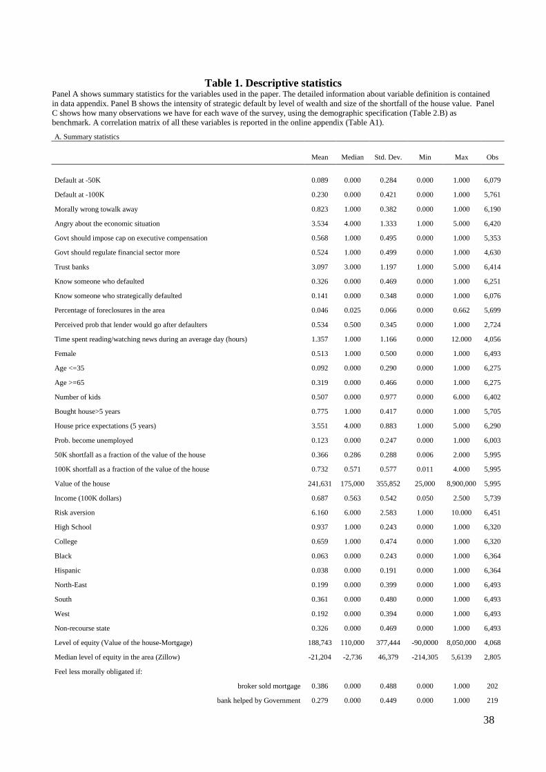
38

Table 1. Descriptive statistics

Panel A shows summary statistics for the variables used in the paper. The detailed information about variable definition is contained in data appendix. Panel B shows the intensity of strategic default by level of wealth and size of the shortfall of the house value. Panel C shows how many observations we have for each wave of the survey, using the demographic specification (Table 2.B) as benchmark. A correlation matrix of all these variables is reported in the online appendix (Table A1).

A. Summary statistics Mean Median Std. Dev. Min Max Obs Default at -50K 0.089 0.000 0.284 0.000 1.000 6,079

Default at -100K 0.230 0.000 0.421 0.000 1.000 5,761

Morally wrong towalk away 0.823 1.000 0.382 0.000 1.000 6,190

Angry about the economic situation 3.534 4.000 1.333 1.000 5.000 6,420

Govt should impose cap on executive compensation 0.568 1.000 0.495 0.000 1.000 5,353

Govt should regulate financial sector more 0.524 1.000 0.499 0.000 1.000 4,630

Trust banks 3.097 3.000 1.197 1.000 5.000 6,414

Know someone who defaulted 0.326 0.000 0.469 0.000 1.000 6,251

Know someone who strategically defaulted 0.141 0.000 0.348 0.000 1.000 6,076

Percentage of foreclosures in the area 0.046 0.025 0.066 0.000 0.662 5,699

Perceived prob that lender would go after defaulters 0.534 0.500 0.345 0.000 1.000 2,724

Time spent reading/watching news during an average day (hours) 1.357 1.000 1.166 0.000 12.000 4,056

Female 0.513 1.000 0.500 0.000 1.000 6,493

Age <=35 0.092 0.000 0.290 0.000 1.000 6,275

Age >=65 0.319 0.000 0.466 0.000 1.000 6,275

Number of kids 0.507 0.000 0.977 0.000 6.000 6,402

Bought house>5 years 0.775 1.000 0.417 0.000 1.000 5,705

House price expectations (5 years) 3.551 4.000 0.883 1.000 5.000 6,290

Prob. become unemployed 0.123 0.000 0.247 0.000 1.000 6,003

50K shortfall as a fraction of the value of the house 0.366 0.286 0.288 0.006 2.000 5,995

100K shortfall as a fraction of the value of the house 0.732 0.571 0.577 0.011 4.000 5,995

Value of the house 241,631 175,000 355,852 25,000 8,900,000 5,995

Income (100K dollars) 0.687 0.563 0.542 0.050 2.500 5,739

Risk aversion 6.160 6.000 2.583 1.000 10.000 6,451

High School 0.937 1.000 0.243 0.000 1.000 6,320

College 0.659 1.000 0.474 0.000 1.000 6,320

Black 0.063 0.000 0.243 0.000 1.000 6,364

Hispanic 0.038 0.000 0.191 0.000 1.000 6,364

North-East 0.199 0.000 0.399 0.000 1.000 6,493

South 0.361 0.000 0.480 0.000 1.000 6,493

West 0.192 0.000 0.394 0.000 1.000 6,493

Non-recourse state 0.326 0.000 0.469 0.000 1.000 6,493

Level of equity (Value of the house-Mortgage) 188,743 110,000 377,444 -90,0000 8,050,000 4,068

Median level of equity in the area (Zillow) -21,204 -2,736 46,379 -214,305 5,6139 2,805

Feel less morally obligated if:

broker sold mortgage 0.386 0.000 0.488 0.000 1.000 202

bank helped by Government 0.279 0.000 0.449 0.000 1.000 219

39

bank involved in predatory lending 0.435 0.000 0.497 0.000 1.000 207

B. Fraction defaulting strategically by value of wealth and size of the shortfall House value Shortfall at Change in default probability when shortfall increases: 50K 100K 150K from 0 a 50 from 50 a 100 from 100 a 150 <100 K 0.144 0.359 0.528 0.144 0.215 0.169 100-200 K 0.113 0.278 0.444 0.113 0.165 0.166 200 -400 K 0.086 0.190 0.311 0.086 0.104 0.121 >400 K 0.067 0.168 0.308 0.067 0.101 0.140

C. Number of observations per wave

Wave 1 434 2 575 3 534 4 533 5 619 6 542 7 494 8 428 Total 4159

40

Table 2. Demographic determinants of the decision to default strategically

The dependent variable is a dummy equal to one if the homeowner says s/he is willing to default when the value of his home equity equal -50K (in Panel A) or -100K (in Panel B) even if s/he can afford to pay the monthly mortgage costs. All the other variables are defined in Table 1. The reported coefficients are marginal effects estimated with a probit model and computed at the mean of the independent variables. All the regressions contain a constant term (not reported) and dummies for waves. Robust standard errors are in brackets. */**/*** indicates statistical significance at the 10%, 5%, and 1% level.

A. Walk away at -50k

(1) (2) (3) (4) (5)

Black 0.077*** 0.064*** 0.063*** 0.063*** 0.064***

(0.020) (0.019) (0.019) (0.022) (0.022)

Hispanic 0.073*** 0.058** 0.062** 0.085*** 0.083***

(0.025) (0.025) (0.025) (0.031) (0.031)

North-East -0.024** -0.017* -0.018* -0.011 -0.010

(0.009) (0.010) (0.010) (0.011) (0.012)

South -0.022** -0.018** -0.014 -0.008 -0.009

(0.009) (0.009) (0.009) (0.010) (0.011)

West -0.028*** -0.018* -0.017 -0.024** -0.025**

(0.009) (0.010) (0.010) (0.011) (0.012)

Female -0.037*** -0.037*** -0.038*** -0.041*** -0.038***

(0.007) (0.008) (0.008) (0.008) (0.008)

High school -0.006 -0.003 -0.005 -0.003

(0.016) (0.016) (0.018) (0.018)

College -0.009 -0.010 -0.003 -0.004

(0.009) (0.009) (0.010) (0.010)

Shortfall % house 0.095*** 0.095*** 0.079*** 0.080***

(0.011) (0.011) (0.013) (0.013)

Age<=35 0.021 0.022 0.021

(0.015) (0.016) (0.016)

Age>=65 0.017* 0.026** 0.028**

(0.009) (0.011) (0.011)

Kids -0.001 -0.003 -0.003

(0.004) (0.004) (0.004)

Bought>5 years -0.016 -0.015

(0.011) (0.011)

House price expectation -0.002 -0.003

(0.005) (0.005)

Prob. become unemployed 0.048*** 0.047***

(0.015) (0.015)

Income (100K dollars) -0.019* -0.019*

(0.010) (0.010)

Risk Aversion -0.002

(0.002)

Non-recourse State 0.005

41

(0.010)

Observations 5,973 5,460 5,280 4,171 4,159

B. Walk away at -100k (1) (2) (3) (4) (5) Black 0.105*** 0.091*** 0.095*** 0.103*** 0.106*** (0.026) (0.027) (0.027) (0.031) (0.032) Hispanic 0.094*** 0.096*** 0.110*** 0.141*** 0.138*** (0.033) (0.034) (0.035) (0.041) (0.041) North-East -0.037** -0.025 -0.026 0.000 0.001 (0.016) (0.017) (0.017) (0.020) (0.020) South -0.021 -0.017 -0.015 -0.002 -0.003 (0.014) (0.015) (0.015) (0.017) (0.018) West -0.062*** -0.050*** -0.050*** -0.038** -0.040* (0.016) (0.017) (0.017) (0.019) (0.021) Female -0.019 0.004 0.012 0.038 0.038 (0.025) (0.025) (0.025) (0.027) (0.028) High school -0.065*** -0.038*** -0.034** -0.016 -0.016 (0.013) (0.014) (0.014) (0.016) (0.016) College -0.047*** -0.056*** -0.057*** -0.067*** -0.066*** (0.011) (0.012) (0.012) (0.013) (0.013) Shortfall % house 0.199*** 0.195*** 0.157*** 0.161*** (0.020) (0.021) (0.024) (0.024) Age<=35 0.071*** 0.068*** 0.067** (0.023) (0.026) (0.026) Age>=65 0.051*** 0.052*** 0.055*** (0.015) (0.017) (0.018) Kids -0.016** -0.016** -0.016** (0.007) (0.007) (0.007) Bought>5 years -0.026 -0.025 (0.017) (0.017) House price expectation -0.007 -0.006 (0.008) (0.008) Prob. become unemployed 0.080*** 0.080*** (0.026) (0.026) Income (100K dollars) -0.073*** -0.073*** (0.015) (0.015) Risk Aversion -0.002 (0.003) Non-recourse State 0.008 (0.017) Observations 5,527 5,189 5,023 3,981 3,969

42

Table 3. The effect of morality on strategic default The dependent variable is a dummy equal to one if the homeowner says s/he is willing to default when the value of his home equity equal -50K (in Panel A) or -100K (in Panel B) even if s/he can afford to pay the monthly mortgage costs. All the other variables are defined in Table 1. In Panel A, Columns (1), (2), (5) the reported coefficients are marginal effects estimated with a probit model (IV-probit in column (5)) computed at the mean of the independent variables. In columns (3), (4), and (7) the reported coefficients are marginal effects estimated with a linear probability model (LPM). In the IV estimates “default is morally wrong” is instrumented with an indicator variable on whether the respondent is a Republican. For Columns (6) and (7), we use only the observations where the morality question is asked at the beginning. In Panel C, column 1 and 2, we split the sample between people declaring positive and negative equity according to the survey. In Columns 3 and 4 we have split the sample between people with positive and negative equity, using data on median negative equity in the metropolitan area (Zillow). Not all the people live in a metropolitan area, and Zillow does not provide data for every metropolitan area. In Columns 5 and 6 we have split the sample according to the size of the drop in house price at state level distinguishing between below and above median (data from FHFA). All the regressions contain a constant term (reported only for linear specification) and dummies for waves. Robust standard errors are in brackets. */**/*** indicates statistical significance at the 10%, 5%, and 1% level. A. Walk away at -50k

Probit IV: First and Second Stage LPM LPM

BOOTSTRAP (1) (2) (3) (4) (5) (6) (7)

Morally wrong to walk away -0.099*** -2.475*** -0.105*** -0.080*** -0.067** (0.015) (0.226) (0.015) (0.025) (0.028) Shortfall % house 0.080*** 0.079*** 0.316** -0.020 0.123*** 0.079*** (0.013) (0.013) (0.126) (0.025) (0.022) (0.029) House price expectation -0.003 -0.002 -0.003 0.005 -0.001 0.006 (0.005) (0.005) (0.026) (0.007) (0.006) (0.008) Prob. become unemployed 0.047*** 0.042*** 0.173* -0.010 0.048** -0.021 (0.015) (0.015) (0.097) (0.025) (0.019) (0.021) Income (100K dollars) -0.019* -0.018* -0.010 0.029** -0.009 -0.008 (0.010) (0.010) (0.054) (0.012) (0.009) (0.013) Bought>5 years -0.015 -0.017 -0.108* -0.014 -0.019* -0.015 (0.011) (0.011) (0.056) (0.014) (0.011) (0.018) Risk Aversion -0.002 -0.003 -0.020** -0.003 -0.003* -0.004 (0.002) (0.002) (0.009) (0.003) (0.002) (0.003) Non-recourse State 0.005 0.006 0.023 -0.001 0.007 -0.001 (0.010) (0.010) (0.057) (0.015) (0.011) (0.015) Republican 0.059*** (0.012) Other controls YES YES YES YES YES YES Constant 1.324*** 0.842*** 0.187*** 0.146** (0.432) (0.051) (0.043) (0.064) Observations 4,159 4,059 3,969 3,969 4,059 1,357

43

B. Walk away at -100k

Probit IV: First and Second Stage LPM LPM

BOOTSTRAP (1) (2) (3) (4) (7) (8) (7)

Morally wrong to walk away -0.201*** -2.232*** -0.198*** -0.169*** -0.110*** (0.021) (0.361) (0.020) (0.035) (0.037) Shortfall % house 0.161*** 0.164*** 0.376*** -0.027 0.194*** 0.143*** (0.024) (0.024) (0.126) (0.026) (0.028) (0.043) House price expectation -0.006 -0.005 -0.004 0.006 -0.005 0.010 (0.008) (0.008) (0.025) (0.008) (0.008) (0.013) Prob. become unemployed 0.080*** 0.072*** 0.180** -0.004 0.069** -0.024 (0.026) (0.026) (0.088) (0.025) (0.027) (0.038) Income (100K dollars) -0.073*** -0.073*** -0.139** 0.027** -0.051*** -0.049*** (0.015) (0.015) (0.066) (0.013) (0.012) (0.017) Bought>5 years -0.025 -0.026 -0.092* -0.015 -0.027* -0.007 (0.017) (0.017) (0.051) -0.015 (0.016) (0.026) Risk Aversion -0.002 -0.002 -0.011 -0.003 -0.002 -0.006 (0.003) (0.003) (0.008) (0.003) (0.003) (0.004) Non-recourse State 0.008 0.008 0.014 -0.003 0.010 0.007 (0.017) (0.017) (0.053) (0.015) (0.016) (0.025) Republican 0.056*** (0.012) Other controls YES YES YES YES YES YES Constant 1.310*** 0.830*** 0.379*** 0.308*** (0.455) (0.052) (0.059) (0.097) Observations 3,969 3,889 3,804 3,804 3,889 1,308

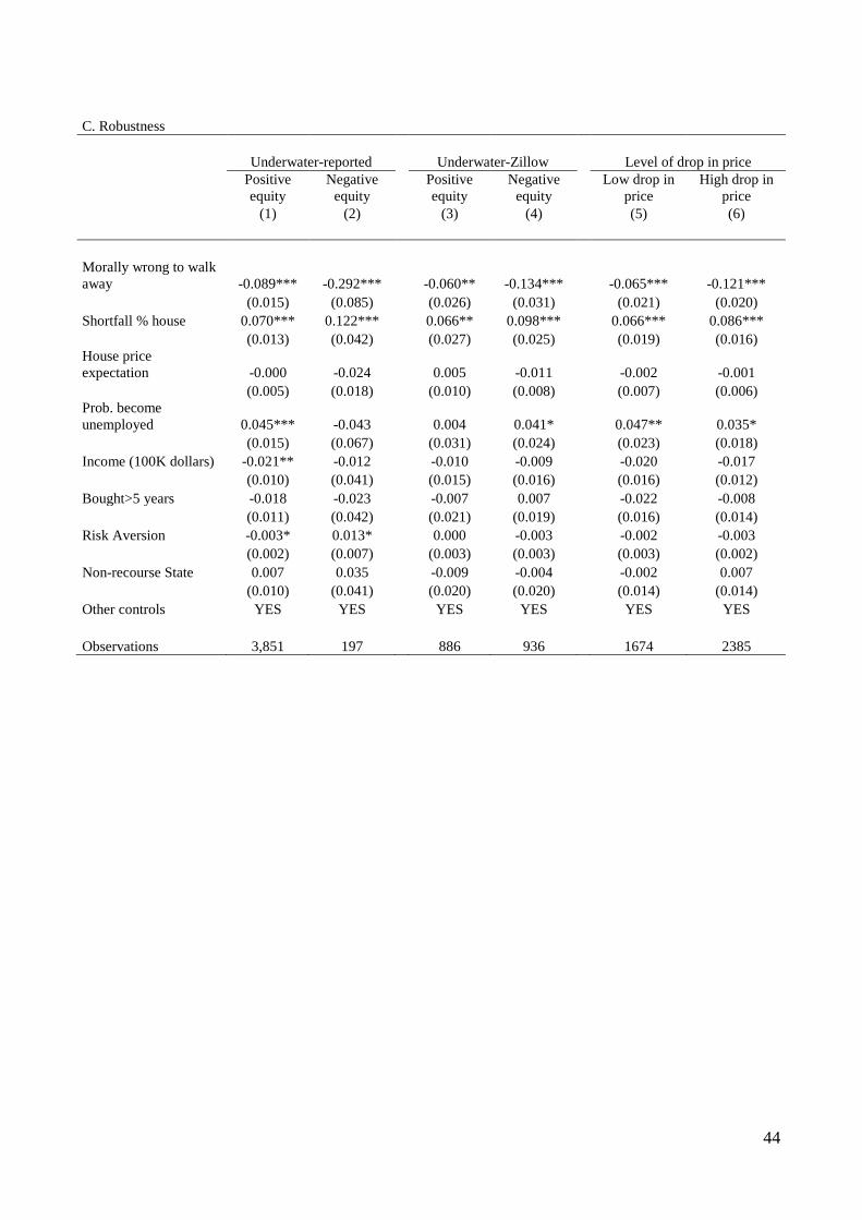
44

C. Robustness Underwater-reported Underwater-Zillow Level of drop in price

Positive equity

Negative equity Positive

equity Negative

equity Low drop in price

High drop in price

(1) (2) (3) (4) (5) (6) Morally wrong to walk away -0.089*** -0.292*** -0.060** -0.134*** -0.065*** -0.121*** (0.015) (0.085) (0.026) (0.031) (0.021) (0.020) Shortfall % house 0.070*** 0.122*** 0.066** 0.098*** 0.066*** 0.086*** (0.013) (0.042) (0.027) (0.025) (0.019) (0.016) House price expectation -0.000 -0.024 0.005 -0.011 -0.002 -0.001 (0.005) (0.018) (0.010) (0.008) (0.007) (0.006) Prob. become unemployed 0.045*** -0.043 0.004 0.041* 0.047** 0.035* (0.015) (0.067) (0.031) (0.024) (0.023) (0.018) Income (100K dollars) -0.021** -0.012 -0.010 -0.009 -0.020 -0.017 (0.010) (0.041) (0.015) (0.016) (0.016) (0.012) Bought>5 years -0.018 -0.023 -0.007 0.007 -0.022 -0.008 (0.011) (0.042) (0.021) (0.019) (0.016) (0.014) Risk Aversion -0.003* 0.013* 0.000 -0.003 -0.002 -0.003 (0.002) (0.007) (0.003) (0.003) (0.003) (0.002) Non-recourse State 0.007 0.035 -0.009 -0.004 -0.002 0.007 (0.010) (0.041) (0.020) (0.020) (0.014) (0.014) Other controls YES YES YES YES YES YES Observations 3,851 197 886 936 1674 2385

45

Table 4: Change in morality The dependent variable is a dummy equal to one if the homeowner says s/he would feel less morally obligated to repay the mortgage if one particular situation occurs (the broker has sold the mortgage, the bank has received money from the government, the bank was accused of predatory lending). All the other variables are defined in Table 1. These data are collected starting only from the 8th wave. One of the three situations is randomly assigned to the individual. The reported coefficients are marginal effects estimated with a probit model and computed at the mean of the independent variables. All the regressions contain a constant term (not reported) and dummies for waves. Robust standard errors are in brackets. */**/*** indicates statistical significance at the 10%, 5%, and 1% level. Broker who sells Bank helped Predatory (1) (2) (3) Morally wrong to walk away -0.325** -0.326** -0.022 (0.131) (0.155) (0.118) Shortfall % house -0.303* -0.157 0.076 (0.182) (0.129) (0.192) House price expectation 0.046 0.108*** 0.101* (0.050) (0.040) (0.059) Prob. become unemployed -0.257 0.198 0.037 (0.205) (0.140) (0.205) Income (100K dollars) -0.266 -0.684*** -0.145 (0.184) (0.216) (0.191) Bought>5 years 0.228*** -0.078 -0.239* (0.085) (0.125) (0.133) Risk Aversion 0.032* 0.021 0.005 (0.018) (0.016) (0.022) Non-recourse State -0.175* 0.132 0.166 (0.100) (0.100) (0.127) Other controls YES YES YES Observations 136 147 127

46

Table 5. Anger, trust, and strategy defaults

The dependent variable is a dummy equal to one if the homeowner says s/he is willing to default when the value of his home equity equals -50K (in Panel A) or -100K (in Panel B) even if s/he can afford to pay the monthly mortgage costs. All the other variables are defined in Table 1. The reported coefficients are marginal effects estimated with a probit model and computed at the mean of the independent variables. All the regressions contain a constant term (not reported) and dummies for waves. Robust standard errors are in brackets. */**/*** indicates statistical significance at the 10%, 5%, and 1% level. A. Walk away at -50k (1) (2) (3) (4) Angry about the economic situation 0.012*** (0.003) Trust banks -0.013*** (0.003) Govt should impose cap on 0.028***

executive compensation (0.009) Govt should regulate financial 0.025***

sector more (0.009) Morally wrong to walk away -0.099*** -0.095*** -0.097*** -0.093*** (0.015) (0.014) (0.016) (0.017) Shortfall % house 0.081*** 0.079*** 0.078*** 0.072*** (0.012) (0.012) (0.013) (0.014) House price expectation 0.000 0.001 -0.001 -0.002 (0.005) (0.005) (0.005) (0.005) Prob. become unemployed 0.038** 0.039*** 0.032** 0.025 (0.015) (0.015) (0.016) (0.017) Income (100K dollars) -0.016* -0.019** -0.019* -0.021* (0.010) (0.010) (0.010) (0.011) Bought>5 years -0.017 -0.016 -0.015 -0.024* (0.010) (0.010) (0.011) (0.013) Risk Aversion -0.003* -0.003** -0.002 -0.003 (0.002) (0.002) (0.002) (0.002) Non-recourse State 0.007 0.005 0.005 0.008 (0.010) (0.010) (0.011) (0.012) Other controls YES YES YES YES Observations 4,039 4,034 3,375 2,958

47

B. Walk away at -100k (1) (2) (3) (4) Angry about the economic situation 0.019*** (0.005) Trust banks -0.016*** (0.006) Govt should impose cap on 0.073***

executive compensation (0.015) Govt should regulate financial 0.066***

sector more (0.016) Morally wrong to walk away -0.200*** -0.199*** -0.201*** -0.190*** (0.021) (0.021) (0.022) (0.024) Shortfall % house 0.169*** 0.166*** 0.153*** 0.149*** (0.024) (0.024) (0.025) (0.027) House price expectation -0.003 -0.001 -0.009 -0.009 (0.008) (0.008) (0.008) (0.009) Prob. become unemployed 0.066** 0.065** 0.051* 0.050* (0.026) (0.026) (0.028) (0.029) Income (100K dollars) -0.070*** -0.075*** -0.081*** -0.087*** (0.015) (0.015) (0.016) (0.017) Bought>5 years -0.026 -0.023 -0.023 -0.020 (0.017) (0.017) (0.019) (0.020) Risk Aversion -0.002 -0.003 -0.001 -0.002 (0.003) (0.003) (0.003) (0.003) Non-recourse State 0.008 0.009 0.018 0.028 (0.017) (0.017) (0.018) (0.020) Observations 3,871 3,868 3,234 2,846

48

Table 6. Defaults and information about other defaulters

The dependent variable is a dummy equal to one if the homeowner says s/he is willing to default when the value of his home equity equal -50 (in Panel A) or -100K (in Panel B) even if s/he can afford to pay the monthly mortgage costs. All the other variables are defined in Table 1. The reported coefficients are marginal effects estimated with a probit model and computed at the mean of the independent variables. All the regressions contain a constant term (not reported) and dummies for waves. Robust standard errors are in brackets. */**/*** indicates statistical significance at the 10%, 5%, and 1% level. A. Walk away at -50k (1) (2) (3) (4) (5) Know someone who strategically defaulted 0.045*** 0.043*** 0.041** 0.037** (0.013) (0.013) (0.017) (0.017) Percentage of foreclosures in the area 0.163*** 0.158*** 0.162*** (0.060) (0.060) (0.060) Know someone who defaulted 0.004 0.021** 0.006 (0.011) (0.009) (0.011) Morally wrong to walk away -0.099*** -0.086*** -0.100*** -0.090*** -0.086*** (0.015) (0.015) (0.015) (0.015) (0.015) Angry about the economic situation 0.011*** 0.013*** 0.010*** 0.014*** 0.013*** (0.003) (0.003) (0.003) (0.003) (0.003) Shortfall % house 0.082*** 0.082*** 0.082*** 0.083*** 0.082*** (0.013) (0.013) (0.013) (0.013) (0.013) House price expectation 0.002 0.003 0.002 0.003 0.003 (0.005) (0.005) (0.005) (0.005) (0.005) Prob. become unemployed 0.040*** 0.043*** 0.039*** 0.041*** 0.042*** (0.015) (0.015) (0.015) (0.015) (0.015) Income (100K dollars) -0.018* -0.015 -0.018* -0.013 -0.015 (0.010) (0.010) (0.010) (0.010) (0.010) Bought>5 years -0.019* -0.020* -0.019* -0.019* -0.020* (0.011) (0.011) (0.011) (0.011) (0.011) Risk Aversion -0.003 -0.001 -0.003 -0.001 -0.001 (0.002) (0.002) (0.002) (0.002) (0.002) Non-recourse State 0.004 0.003 0.004 0.004 0.003 (0.010) (0.011) (0.010) (0.011) (0.011) Other controls YES YES YES YES YES Observations 3,847 3,459 3,847 3,541 3,459

49

B. Walk away at -100k (1) (2) (3) (4) (5) Know someone who strategically defaulted 0.035* 0.032 0.033 0.027 (0.020) (0.020) (0.025) (0.025) Percentage of foreclosures in the area 0.195* 0.187* 0.194* (0.115) (0.112) (0.115) Know someone who defaulted 0.002 0.018 0.007 (0.019) (0.015) (0.019) Morally wrong to walk away -0.199*** -0.193*** -0.199*** -0.199*** -0.193*** (0.021) (0.022) (0.021) (0.022) (0.022) Angry about the economic situation 0.018*** 0.018*** 0.018*** 0.019*** 0.018*** (0.005) (0.006) (0.005) (0.006) (0.006) Shortfall % house 0.170*** 0.161*** 0.170*** 0.162*** 0.161*** (0.025) (0.027) (0.025) (0.027) (0.027) House price expectation -0.000 0.002 -0.000 0.000 0.002 (0.008) (0.008) (0.008) (0.008) (0.008) Prob. become unemployed 0.063** 0.063** 0.063** 0.065** 0.062** (0.027) (0.028) (0.027) (0.028) (0.028) Income (100K dollars) -0.069*** -0.063*** -0.069*** -0.065*** -0.063*** (0.016) (0.016) (0.016) (0.016) (0.016) Bought>5 years -0.030* -0.039** -0.030* -0.035* -0.039** (0.018) (0.019) (0.018) (0.019) (0.019) Risk Aversion -0.002 -0.002 -0.002 -0.002 -0.002 (0.003) (0.003) (0.003) (0.003) (0.003) Non-recourse State 0.009 0.001 0.009 -0.002 0.001 (0.017) (0.018) (0.017) (0.018) (0.018) Other controls YES YES YES YES YES Observations 3,691 3,321 3,691 3,399 3,321

50

Table 7 Determinants of the probability that lenders go after defaulters

The dependent variable is the perceived probability that a lender would go after defaulters, measured on a scale between 0 and 100. The table reports beta coefficients from OLS regressions. All the regressions contain dummies for waves. Robust standard errors are in brackets. */**/*** indicates statistical significance at the 10%, 5%, and 1% level.

Perceived probability that the lender would go after defaulters

(1) (2) (3)

Know someone who strategically defaulted -0.088*** -0.060** (0.021) (0.026) Know someone who defaulted -0.065*** -0.039* (0.016) (0.021) Shortfall % house 0.013 0.015 0.014 (0.029) (0.029) (0.029) House price expectation 0.002 0.006 0.002 (0.010) (0.010) (0.010) Prob. become unemployed 0.096*** 0.093*** 0.097*** (0.032) (0.032) (0.032) Income (100K dollars) -0.044** -0.037** -0.043** (0.018) (0.017) (0.018) Bought>5 years 0.013 0.009 0.013 (0.020) (0.020) (0.020) Risk Aversion -0.004 -0.003 -0.004 (0.003) (0.003) (0.003) Non-recourse State -0.011 -0.008 -0.010 (0.019) (0.019) (0.019) Constant 0.514*** 0.492*** 0.519*** (0.063) (0.064) (0.063) Other controls YES YES YES Observations 1,852 1,890 1,852

51

Table 8. The role of the media in explaining strategic defaults The dependent variable is a dummy equal to one if the homeowner says s/he is willing to default when the value of his home equity equal -50K even if s/he can afford to pay the monthly mortgage costs. All the other variables are defined in Table 1. Since data on the media were collected starting with wave 4, estimates are based on waves 4-8. The reported coefficients are marginal effects estimated with a probit model and computed at the mean of the independent variables. All the regressions contain a constant term and dummies for waves. Robust standard errors are in brackets. */**/*** indicates statistical significance at the 10%, 5%, and 1% level. Walk away at -50k (waves 4-8) (1) (2) (3) (4) (5) (6) Time spent reading/watching news 0.008* 0.034* 0.009* 0.038** 0.009** 0.038**

during an average day (hours) (0.004) (0.018) (0.005) (0.018) (0.005) (0.018) Wave 0.003 0.005 0.007 (0.006) (0.006) (0.006) Time news*wave -0.005 -0.005* -0.005* (0.003) (0.003) (0.003) Know someone who strategically defaulted 0.048*** 0.049*** 0.065*** 0.065*** (0.016) (0.016) (0.024) (0.024) Know someone who defaulted -0.016 -0.016 (0.015) (0.015) Percentage of foreclosures in the area 0.133 0.131 0.135 0.131 (0.084) (0.084) (0.084) (0.083) Shortfall % house 0.077*** 0.076*** 0.075*** 0.073*** 0.075*** 0.075*** (0.016) (0.016) (0.018) (0.018) (0.018) (0.018) House price expectation -0.005 -0.004 -0.004 -0.004 -0.005 -0.004 (0.006) (0.006) (0.007) (0.007) (0.007) (0.007) Prob. become unemployed 0.032 0.031 0.041** 0.040** 0.042** 0.042** (0.020) (0.020) (0.020) (0.020) (0.020) (0.020) Income (100K dollars) -0.003 -0.004 -0.011 -0.012 -0.011 -0.010 (0.012) (0.011) (0.013) (0.012) (0.013) (0.013) Bought>5 years -0.005 -0.006 -0.012 -0.012 -0.011 -0.011 (0.014) (0.014) (0.015) (0.015) (0.015) (0.015) Risk Aversion -0.002 -0.002 -0.001 -0.001 -0.002 -0.001 (0.002) (0.002) (0.002) (0.002) (0.002) (0.002) Non-recourse State 0.004 0.004 0.006 0.006 0.006 0.006 (0.013) (0.013) (0.014) (0.014) (0.014) (0.014) Other controls YES YES YES YES YES YES Observations 2,616 2,616 2,214 2,214 2,214 2,214