RESEARCH BULLETIN 1076

The Demand for land in the Urban-Rural Fringe

LEROY J. HUSHAK

GARY N. BOVARD

JANUARY 1975

OHIO AGRICULTURAL RESEARCH AND DEVELOPMENT CENTER

Wooster, Ohio

CONTENTS

* * * * *

Introduction ______________________________________________________ 3

Land Use Changes in the Urban-Rural Fringe ____________________________ 3

Urban Demand for Undeveloped Land _________________________________ 4 Size _________________________________________________________ 5

Distance from Urban Center_____________________________________ 5

Location _____________________________________________________ 6

Distance from Highway _______ --------------------------------- 6

Distance from Railroad _________________________________________ 6

Zoning _______________________________________________________ 6

Property Tax Policy ____________________________________________ 7

Characteristics of the Study Area and Data ______________________________ 7

Population ___________________________________________________ 8

Collection and Sources of Data ___________________________________ 9

Characteristics of the Sample ____________________________________ 9

Estimates and Analysis of the Demand for Urban-Rural Fringe Land __________ 10

Estimated Results for Total Sample ________________________________ 13

Estimated Results for Franklin County ______________________________ 15

Conclusions and Imp Ii cations ________________________________________ 17

Conclusions ___________________________________________________ 17

Policy Implications _____________________________________________ 18

Issues for Further Study _________________________________________ 19

Literature Cited __________________ . _________________________________ l 9

AGDEX 822-882-884 1-75-2.SM

THE DEMAND FOR LAND IN THE URBAN-RURAL FR~NGE I

LEROY J. HUSHAK and GARY N. BOVARD2

INTRODUCTION The objective of this study is to estimate and

analyze the impact of urban factors on the market for undeveloped land in the urban-rural fringe. The urban-rural fringe includes land along the boundaries of a city, in the suburbs, in small incorporated towns near the city, and extending into the unincorporated, partially developed countryside surrounding the city. It is the area where land is in transition from agri­cultural to urban use. Undeveloped land from an urban viewpoint is land which is not part of a devel­opment project. The land may and often does have buildings on it.

This land market is basically a private market subject to public controls such as zoning and taxation. Emerging land use problems, such as the difficulty of extending urban services to increasingly dispersed urban activity and unprofitable agriculture near ur­ban centers because of rising property tax assessments, will likely lead to increased public control of land use. Federal and state land use planning legislation is emerging. Various forms of preferential assessment of agricultural land have been adopted in many states ( 8, p. 1 ) . These and other policies are in response to increasing public concern for land use problems. It will be difficult to implement the public interest unless new policies are based on a more complete un­derstanding of the impact which current and poten­tial land use regulations have on the land market. The impact of zonirig and the property tax are ana­lyzed in this study.

The objective of this study is accomplished through the development of an urban demand for land model, and the estimation and analysis of this model for the urban-rural fringe land market sur­rounding Columbus, Ohio. First, aspects of growth in the urban-rural fringe are described and some of the policy problems in the fringe area are outlined. Second, an urban demand for land model with hypo­theses about the expected impacts of land character­istics, zoning, and the property tax on land prices is developed. Third, descriptions are provided of the study area (Franklin County, its urban center, Co-

1Support for this project was provided under Hatch 477, Analysis of the Market for Farm and Rural Real Estate and Forces Determining Land Prices in Ohio, a research project at the Ohio Agricultural Re­search and Development Center. This bulletin is derived from the Master's thesis of the same title by Gary N. Bovard (1973).

2Associate Professor and former Graduate Research Associate, respectively, The Ohio State University and Ohio Agricultural Research and Development ~enter.

3

lumbus, and parts of the six counties surrounding Franklin County), the data collection procedures, and the characteristics of the 225 observations col­lected on 1972 land transactions in the study area. Fourth, the statistical estimates and their analyses are presented. Finally, the conclusions of the study and the resulting policy recommendations are developed.

This study is unique for two reasons. First, it goes beyond previous studies conceptually in its de­velopment of a supply-demand model for land. Sec­ond, it is one of the few studies which use actual land transactions as observations.

LAND USE CHANGES IN THE URBAN-RURAL FRINGE

The United States is becoming an increasingly urbanized nation. Clawson states: "In the last few years, urbanization has occurred largely in the urban­rural fringes. Growth rate of the central cities has slowed, while the areas around them have grown at a remarkable rate" (2, p. 5).

The 1970 Census of Population shows that 13 out of the 25 largest cities had decreases in popula­tion between 1960and1970 (10, p. 147). At the same time, 24 out of the 25 largest metropolitan areas had increases in population ( 10, p. 154) '.

Many factors have increased the importance of the urban-rural fringe land market. These factors include population growth, the dispersion of business. activity, speculation, more highways and recreational facilities, and the zoning and taxing policies of many communities.

The population in the fringe areas has been ris­ing for three reasons. The first is natural population growth. The 1970 Census showed 205 million people in the United States. Despite a declining birth ·rate, there will be a substantial increase in population ( pos­sibly 50 to 80 million) by the year 2000. Much of this growth will locate in the suburbs and fringe areas. Secondly, people are moving away from the cities and into the suburbs. Increased affluence and mobility make it possible for them to move to the suburbs. For these people, the suburbs offer lower home prices, less crime, less congestion, and less pollution. Rural to urban migration is the third reason. People leave their rural communities looking for jobs, a better education, the benefits of urban life, or because they can no longer afford to farm. Although the magni-

tude of rural to urban migration has declined, it is still a factor in urban population growth.

Businesses are also moving to the suburbs and fringe areas. It is advantageous for a business to be located near its work force and consumers. Between 1965 and 1970, New York City lost more than 3,000 manufacturing, retail, and wholesale businesses. De­troit lost 3,500 and Philadelphia nearly 3,000 ( 1, p. 138). Most of them relocated in the suburbs. A business is usually looking for land adjacent to a ma­jor urban access highway and located in a densely populated area. Such a location makes the business more acc~ssible to its workers and customers, and re­duces shipping and receiving costs.

Rising land values in the urban-rural fringe pro­vide an incentive for land speculation. A speculator is interested in buying and holding undeveloped land which is expected to gain in value at relatively rapid rates. He is in competition with developers and businesses. Although speculation does not cause ris­ing land values, it does contribute to the rate at which they increase.

One result of speculation in the urban-rural fringe is idle land. Often a speculator will hold land for several years before selling. He can do this be­cause the costs of holding the land, such as opportun­ity costs of invested funds and property taxes, are relatively low compared to the expected gains from holding the property. The speculator wi~l hold the land until offered a price at which expected future gains are less than those from alternative investment opportunities, perhaps in other tracts of land. When the offer price of a tract of land or the expectation of a particular speculator is high compared to other land around that property, developers. will skip over the high-priced land and develop farther away fron:i the city. The land skipped over is left 1dle until the speculator receives his price. ·

Increased population and increased business activity in the urban-rural fringe require more and better transportation. As people spread out into de­velopments, many of which are separated by idle land, more miles of roads are needed to reach them. Increased traffic also requires improved highways because these people still want to be able to reach the city quickly and easily. The result is an increased amount of fringe land used for new and improved roads. Clawson claims that streets and alleys often occupy a third or more of the land area in urban use (2, p. 145).

With increasing income and more leisure time, there is an increasing demand for recreational land. Furthermore, people want the recreation near their homes. Golf courses, parks, and other outdoor rec­reation areas :equire large an_iou11:~~ ~f la11:d: ...

4.

The quantity of undeveloped land can be in­fluenced by community zoning and taxing policies. Large lot zoning, adopted by many communities dur­ing the 1950's and 1960's, causes excessive dispersion of residential developments. The current property tax encourages idle land. It can be minimized by removing taxable improvements. Further, it is a small cost relative to expected gains from holding land. Dispersed residential areas, idle land, and dis­continuity in development form a condition in fringe areas called sprawl. Community services and trans­portation networks are forced farther from the city, causing increased costs to the public and misuse of fringe land.

Farmers in the urban-rural fringe probably face the most difficult problems from rising land values. Farmers are the recipients of increased value for their land if they hold it as speculators. But they also face increased property taxes as a result of the increased value of their land. The increased property taxes may result in losses from the farm operation and the early selling of the land because of difficulties in financing the increased taxes.

URBAN DEMAND FOR UNDEVELOPED LAND The urban demand model is a micro, point-in­

time model for individual buyers and sellers of unde­veloped land in a single urban center. The micro orientation of the model is addressed to explaining variations across individual land transactions, and not to a buyer's total demand for land nor to an ag­gregate urban . demand for land. The point-in-time framework means that factors affecting expected land productivity (which may change over time) are con­stant. For example, changes in transportation costs affect land prices over. time by changillg .an expected cost factor of land use. At any· point in time, how"'." ev:er., factors such as expected transportation 'costs, expected tax levels, and expected returns from land use alternatives are given. The limitation to a single urban center eliminates the need to incorporate in­terurban factors which affect the land market, such as population, population density, geographical size, and industrial concentration.

The number of undeveloped land parcels and their size and characteristics facing potential buyers at any point in time are given. The number, size, and characteristics of land parcels for any urban cen­ter change over time with changing price and cost expectations, such as changes in economic conditions and the development of roads, residential areas, and industrial and retail centers. However, at any point in time, the numb~r, size, characteristics, and expec­tations about future productivity of land parcels are given. This fixed set of undeveloped land_ par~els

around the urban center constitutes the supply of un­developed land.

Potential land buyers seek to obtain land parcels from current owners. When the present value (price) of a land parcel to one or more land buyers exceeds that of the current owner, a transaction oc­curs between the current owner and the buyer for w horn the price is greatest. 3 The primary role of advertising and real estate dealers is viewed as one of providing information among landowners and buyers about land parcels and market conditions. Real estate dealers also sell services required to complete land transactions. Further, there are no conceptual bounds on the supply of land parcels to the urban­rural fringe land market. The urban demand func­tion for undeveloped land determines which parcels have greater urban than agricultural expected use value at any point in time.

Under conditions of a given supply of land par­cels of given size, characteristics, and future expecta­tions, the locus of land transactions traces the demand function for undeveloped land, i.e., the relationship which determines the maximum price per unit for land parcels with varying sets of characteristics. The general form of the demand function is:

PRICE~ f(SIZE, DCITY, DHGWY, DRR, LOC, ZONE, TAX, X) (1)

where: PRICE= price or value of the land per acre SIZE = size of the land parcel (acres) DCITY = distance of the land from the urban

center (miles) DHGWY = distance of the land from a major·

access highway (miles) DRR = distance of the land from railroad (miles) LOC = location of the land within the incorpo­

rated area of the urban center, with­in the incorporated area of ·a suburb or other incorporated place, or in an unincorporated township

ZONE = zoning or other restrictive use policies to which the land parcel is subject

TAX= property tax structure on the land and X = other characteristics. Other characteristics are factors expected to af­

fect land prices which could not be developed from the data sources available for this study. Informa­tion on topography, trees, or other environmental fac­tors would require on-site inspection. Information on special contract arrangements (e.g., deferred pay­ment or seller financing) would require interviews with persons having direct knowledge of each trans­action. Omission of these factors will not affect the

3The price of land is a present value, i.e., the discounted sum of expected future returns from a land parcel with a given set of char­acteristics. For further discussion of discounted future returns to land, see Downing ·(4).

5·

estim~ted impact of included characteristics on land prices if the omitted factors are uncorrelated with the included factors.

The demand function is conceived as a single relationship for undeveloped land in the urban-rural fringe. All buyers compete for land parcels from the same set or supply of land parcels. However, sev­eral factors, such as zoning, limit future alternatives. The analytical framework incorporates these limita­tions by searching and allowing for interactions such as the impact of commercial zoning on land price through distance from a railroad.

Size Since the unit of observation is a transaction

(not total quantity of land per buyer), the basic price-quantity relationship in the demand function is between price per unit and the size (units) of a land parcel. As size increases, given other character­istics, price is expected to decline. Downing ( 4) in his study of commercial land value found a negative relationship between parcel size and price.

As parcel size increases, the more likely it is that parcel size will exceed a buyer's requirements, and a buyer will pay less for land in excess of his require­ments. Further, the larger the parcel is, the more likely it is to require further subdivision costs. For example, if a business needs 3 acres of land for its op­eration and a parcel will only sell as 4 acres, the busi- · ness will pay very little more total amount for the 4-acre parcel than it would have been willing to pay for a 3-acre parcel. If a home builder wants to buy one-half acre, and the seller cannot or will not sell a parcel of less than 1 acre, the buyer will pay pro­portionately less for the 1-acre parcel than he would have paid for a one-half acre parcel. Parcel size be­comes very important in relation to large lot zoning, which is discussed later. · . . ·

Distance from Urban Center Distance from a major urban center is expected

to have a negative effect on the per unit price of land.4

Schuh and Scharlach ( 9), in their cross-sectional analysis of the value of land and buildings per acre by county in Indiana, found that distance from Chi­cago was negatively related to land value. Hammill ( 6) found a negative relationship between distance from urban centers and rural real estate values in Minnesota counties. Clonts ( 3), in his study of land values in Prince William County, Va., on the periph­ery of Washington, D. C., found that radial mileage to the urban periphery had negative effects on land

4The real concern with respect to an urban center may be the time required to travel from the property to the urban center. How­ever, the use of distance to urban center and distance to a major urban access highway in this study should reasonably approximate time to urban center.

values for all types of land. His study showed that for each additional mile from the urban periphery, the per acre value of unimproved land decreased by about $172. Downing (4) also found a negative re­lationship between land prices and distance from both the central business district and the nearest shopping center.

Both homeowners and businesses pref er land lo­cated closer to the urban center. The benefits of living away from the city, such as fewer people, less traffic, and less noise, must be compared to the ad­vantages of living close to the urban center, the big1.. gest of which is probably transportation. The far­ther from the city a person lives, the greater are the costs and time needed to get into the city.

Businesses also tend to locate close to the city. Retail businesses locate near or in the urban center to attract customers. With such a location, a large number of people pass the business on their way to and from other parts of the city. Manufacturing firms locate close to the city to decrease their costs. Most of their supplies, labor force, and customers are located in the city. Although businesses are moving info the fringe areas, they are not moving very far from the city. The result is higher prices for land located close to a city.

Distance from secondary urban centers is ex­pected to have additional negative, but smaller, ef­fects on land prices. Secondary centers are suburbs and other incorporated municipalities within the ur­ban-rural fringe. The larger secondary centers often include retail business or shopping centers comparable to those of the urban center, which are of particular importance to residential property owners.

Location Land located in the central city and the secon­

dary urban centers is expected to have a higher value than land in the unincorporated townships. The city and secondary centers provide more public ser­vices, such as police, water, and sewer, and may also have better school systems. The value of these ser·­vices is capitalized into land values. The buyer of land has the alternative of purchasing public services through higher land (and tax) prices in incorporated places or purchasing lower priced land in unincor­porated townships and foregoing or providing the services himself.

Distance from Highway The distance from a land parcel to an access

point of a major urban access highway is expected to reduce land prices per acre. Clonts ( 3) found that the distance to an urban access highway had a

. negative effect on land values for all types of land. His study showed that value of undeveloped land de-

creased by $115 per acre for each additional mile from a highway.

Distance to a major highway is especially im­portant to business firms. Direct access to a high­way allows a retail business to be more accessible to its customers. Manufacturers' costs for labor and for shipping and receiving will be decreased because of the ease of reaching their business.

People also prefer living near a major urban ac­cess highway, although not adjacent to it. The clo­ser a person lives to a major urban access highway, the more easily and quickly he can get into the city.

Distance from Railroad The distance from a land parcel to a railroad is

expected to have different effects on land prices for business and residential uses. For a business which does a large amount of shipping and receiving, land adjacent to and having access to a railroad can be extremely valuable if its transportation needs can be fulfilled at less cost by rail. Most business concerns, especially manufacturers and wholesalers, will differ­entiate little between land which is adjacent to a rail­road without access and land farther away from the railroad. Retailers may feel differently about rail­roads, especially if they think customers may be of­f ended by location near a railroad. In such cases, they may wish to be located away from railroads.

The value of residential land is expected to in­crease rapidly as the distance from a railroad in­creases. The effect of a railroad exists until it can no longer be seen or heard. Beyond that point, a railroad should have little or no effect on land values.

Zoning Zoning and tax policies cliff er from the other

factors because they are direct policy variables. The other factors largely represent economic forces in the urban area, although they are influenced by policy decisions affecting the overall development of an ur­ban center in the longer run. However, zoning and tax policies are subject to direct change by political decisions, and as a result may involve more uncer­tainty than the other factors.

Zoning regulations can take many forms. In this study, primary interest is in the impact of com­mercial or multi-family, residential, and agricultural zoning on land prices. The impact of large lot zoning is also discussed. Building codes, health codes, and other restrictive use policies are also likely to have im­pacts on land values.

Generally, zoning is expected to increase land values as it changes from agricultural to residential, and from residential to commercial or multi-family . However, the impact of zoning depends also on the ease or difficulty of changing the zoning on a par-

6. -

ticular property and on other characteristics of the property. For example, if a land parcel is located near a railroad and is zoned residential, its value will be much lower than if it is zoned commercial. If a parcel is located in the center of a heavily populated area, adjacent to a major highway, and zoned com­mercial, its value will probably be much higher than if it is zoned residential.

Large lot zoning requires that all lots meet a minimum size of usually from 1 to 5 acres. Com­munities adopted large lot zoning because they hoped it would help discourage development. The com­munities were afraid that an increased suburban population would put a heavy burden on their ser­vices and on the school system. They further thought it would result in sufficient open recreational space since everyone would have large yards. However, people continued to buy homes despite the large lots.

The cost of community services is "usually higher with large lot zoning than it would be with smaller lots. Since the large lots spread people farther apart, more roads are required to reach them and other ser·­vices must be extended a greater distance. Large lot zoning also does not provide any public recreational value or any true open space. It may reduce the value of the land. As discussed earlier, when a par­cel is larger than a buyer desires, the price per acre is expected to decrease. Since large lot zoning re­quires a certain minimum acreage, it may not be pos­sible for a seller to provide the buyer the size of lot he desires. The result is lower land prices, spread out development, and misuse of fringe land.

Property Tax Policy Local° property tax policies have a variety of ef­

fects on land prices and uses. First, the property tax is expected to have a negative but marginal effect on land prices. The property tax on undeveloped land is small compared to the expected gain in property value over time, especially in a growing urban area. An Illinois study of the effect of property tax displace­ment found that: "Generally, the effects of the tax displacement will be of lesser influence in the market for development properties than in land which con­tinues in a given use, such as farming. In either case, effects on the decisions of speculators are marginar' ( 5, p. 34) . The results of a North Carolina study by Pasour yield a similar conclusion ( 8) .

The small expected effect of the property tax on land values does not imply that the property tax has no important effects, however. The major effects of the property tax are probably on land use, both by farmers and speculators.

The property tax is a tax, not only on the value of land, but on buil~ings and any improvements the

7

landowner makes on the land. A speculator is re­luctant to use idle land in a short-term income pro­viding project, such as a park, because the tax on the improvements may be greater than the income re­ceived from the project. One alternative to the prop­erty tax which might help reduce the idle land prob­lem is the site value tax. The site value tax places a tax only on the value of the land. It does not tax any buildings or improvements made on the land. The site value tax would remove the disincentive to improve land, and more idle land might be used in short-term income generating projects or retained in agriculture.

Farmers in the urban-rural fringe probably face the most difficult problems with the property tax. Tax assessors notice the increasing prices being paid for fringe land and raise the assessment on surround­ing farmland. The increased property taxes may force the farmer to operate at a loss. If the farmer can afford to hold the land until he reaches an optimal selling point, he will gain the same profits realized by speculators plus returns from farming. However, some farmers lack the capital resources to be able to take losses for several years on the land. These farm­ers may be forced to sdl their land long before op­portune selling times have been reached. If the farmer is forced out before he is ready to retire, he must either buy farmland elsewhere or search for a new occupation.

CHARACTERISTICS OF THE STUDY AREA AND DATA

The study area (Fig. 1) includes all of Franklin County, Ohio, and those parts of Union, Fairfield, Madison, Licking, Delaware, and Pickaway counties, locatedo generally within a 25-:-mile radius of City Hall in downtown Columbus, Ohio.

The boundary of the study area was determined by two conditions. First, if more than one-half of a township was within the 25-mile radius, the 0 entire township was included in the study area. If less than one-half was within the 25-mile radius, the entire township was excluded. This procedure was used because there is no information on the location of a land parcel (property) within a township at the State Board of Tax Appeals, the source from which the ob­servations were initially identified.

Second, a township which contained the county seat of a county, except for Franklin County where Columbus is the county seat, was eliminated even if that township was within the 25-mile radius. In each county the county seat was the largest city, and avoiding the direct effect of a property being located in one of these cities was desired.

The study area included 33 townships in the six counties outside of Franklin County. In addition to Columbus, there were seven cities of more than 10,000 population in 1970 in the study area, all lo­cated in Franklin County. In addition, there were four county seat cities of more than 10,000 popula­tion outside of but near the study area whose impact on land values in the study area was incorporated. There were 43 other incorporated municipalities in the study area. Total size of the study area is about 1,6QO square miles.

Population Population in the study area increased by 22.2%

between 1960 and 1970 (Table 1). At the same time, the state of Ohio had a 9.7% increase. Popu­lation in the city of Columbus increased by 14.6%

PICKAWAY

FIG. 1.-Map of study area.

8

from 1960 to 1970 (Table 2), part of which was from expansion of the land area within the city limits. Co­lumbus ranked 21st nationally in populations of U.S. cities in 1970 (10, p. 147). The Columbus metro­politan area increased by 21 % from 754,885 in 1960 to 916,228 in 1970 (10, p. 154). Other cities in Ohio decreased in population: Akron by 5%, Cleve­land by 14%, and Cincinnati by 10%. These re­spective metropolitan areas increased by 12, 8, and 9%.

Several suburban areas had substantial increases in population between 1960 and 1970 (Table 2). Gahanna increased by 356%, Upper Arlington by 58%, and Westerville and Reynoldsburg each in­creased by 79%.

Franklin County alone increased by 22% from 1960 to 1970 (Table 1). No other county involved in the study increased this much. However, the per­centage change for the entire stµdy area outside of Franklin County was 24%, an increase from 68,159 to 84,512. The study area contained 87.2% of the population increase from 1960 to 1970 in the total seven-county area. The study area outside of Frank­lin County contained 40. l % of the population in­crease in the six counties surrounding Franklin County.

Only two towns in the study area outside of Franklin County had populations of more than 2,500 in 1970 (Table 2). Population of Johnstown in Licking County increased by 11.2 % from 1960 to 1970. The population of Sunbury in Delaware

TABLE 1 .-1960 and 1970 Census Populations and Percent Changes, Counties and Study Areas.

Percent County 1960 1970 Change

Franklin 682,962 833,249 22.0 Study Area Same Same Same

Licking 90,242 107,799 19.5 Study Area 14,735 18,545 25.9

Fairfield 63,912 73,301 14.7 Study Area 9,064 12,359 36.4

Delaware 36,107 42,908 18.8 Study Area 13,442 18,406 36.9

Pickaway 35,855 40,071 11.6 Study Area 15, l 17 17,207 13.8

Madison 26,454 28,318 7.0 Study Area 11,838 13,650 15.3

Union 22,853 23,786 4.1 . Study Area 3,963 4,345 9.6

All Counties 958,385 1,149,432 19.9 Study Area 751,121 917,761 22.2

Sources: The 1972 World Almanac [ l 0, p. 206] and U. S. Census of Population, PC(l )-A37 Ohio, 1970.

County increased by 84.7%. Of the county seats, Lancaster in Fairfield County increased by 10% from 1960 to 1970, Delaware in Delaware County by 12.9%, Circleville in Pickaway County by 5.6%, and Newark in Licking County had a very slight increase.

Collection and Sources of Data The sample consists of 225 observations on 1972

land transactions. ·The breakdown of observations by county and the range of dates over whi~h the sample transactions occurred are shown in Table 3.

The sample was stratified on the basis of land area in each county within the sample area to total land area in the sample area, with two exceptions. First, several observations were deleted in the data collection process because their geographical location could not be determined. However, the counties other than Franklin County were expected to be simi­lar, thus not requiring a strict stratification of sample numbers. Second, the number of observations in

TABLE 2.-1960 and 1970 Census Populations and Percent Changes for Cities and Towns of More Than 2,500.

Percent City or Town 1960 1970 Change

Columbus 471,316 540,025 14.6 Newark* 41,790 41,836 0.1 Upper Arlington 24,486 38,630 57.8 Lancaster* 29,916 32,911 10.0 Whitehall 20,818 25,263 21.3 Worthington 9,239 15,326 64.8 Delaware* 13,282 15,008 12.9 Bexley 14,319 14,888 3.9 Reynoldsburg 7;793 13,921 78.6 Westerville 7,011 12,530 78.7 Gahanna 2,717 12,400 356.4 Circleville* 11,059 11,687 5.6 Grandview Heights 8,270 8,460 2.3 Hilliard 5,633 8,369 30.8 Johnstown 2,881 3,208 11.2 Sunbury 1,360 2,512 84.7

*==Not in sample area. Sources: The 1972 World Almanac [ 10, pp. 183-185] and

U. S. Census of Population, PC(l )-A37 Ohio, 1970.

TABLE 3.-Number of Observations by County and the Range of Dates in 1972 During Which the Transactions Occurred.

Number of County Observations Dates

Franklin 65 Jan. 21-April 3 Fairfield 21 Jan. 3 -April 26 Pickaway 27 Jan. 5 -May 11 Licking 22 Jan. 3 -June 7 Union 21 Jan. 14-Aug. 6 Delaware 36 Jan. 11-May 25 Madison 33 Jan. 3 -Sept. 18

225

9

Franklin County was cut by 33 % because: 1) its per­cent of total land area is so large that its observations might dominate the sample too much, and 2) much of its land is platted and not included in this study.5

The other six counties have almost no platted land in the study 'area.

Observations were selected and initial data were collected from the State Board of Tax Appeals. Sales slips were arranged by county and ordered by the date each sale was recorded. Observations were se­lected chronologically, by date of sale, with the elimi­nation of transactions from the sample for two rea­sons. First, all trans·actions of platted land were eliminated because the study is concerned with un­developed land. Second, all transactions are believed to be open market ( arms·-length) cash transactions. Sales made under unusual conditions, to the extent they could be identified, such as sales made· by an executor of a will, through a will, or within families, were excluded.

From the sales slips at the Board of Tax Appeals, information was obtained on: 1) map, parcel, and district numbers used in locating the properties on maps in each county engineer's office; 2) whether the property was located in a city, village, or township (unincorporated area) ; 3) assessed value of the land and buildings on each property at the time of the sale; 4) the selling price; 5) the acreage; and 6) zoning, or if the land was not zoned, the intended use by the new owner.

The exact location of each parcel was determined at the engineer's office in each county. If exact lo­cation could not be determined, the parcel was de­leted from the sample. The exact location was used to plot the observations on a road map. The road map was used to measure distance from Columbus, distance from secondary urban centers, distance from a highway, and distance from a railroad.

Characteristics of the Sample Some of the characteristics of the sample are

presented in Table 4. For the total sample of 225 observations, the average sale value per acre was $14,881, with a range of $111 to $104,839. Of the location variables, land located in secondary urban centers (suburban) was the most valuable, with an average value per acre of $36,068. Commercial property was more valuable than residential or agri­cultural property, with a per acre value of $27 ,641.

Location of land with respect to a railroad, based on the conceptual discussion, is classified as land lo­cated adjacent to a railroad, land located within 0.6 mile of but not adjacent to a railroad, and land lo-

5Platted land has been developed at some time by a developer. The developer has recorded the acreage on a plat map and removed it from the County Auditor's records.

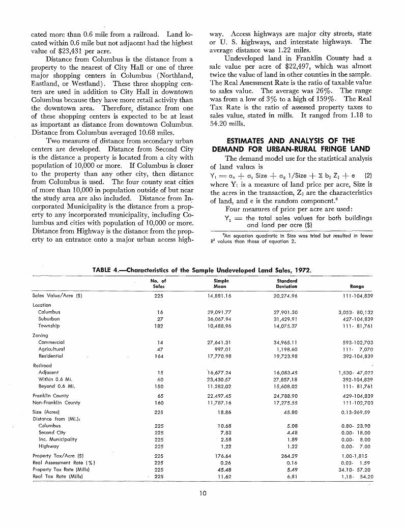
cated more than 0.6 mile from a railroad. Land lo­cated within 0.6 mile but not adjacent had the highest value of $23,431 per acre.

Distance from Columbus is the distance from a property to the nearest of City Hall or one of three major shopping centers in Columbus (Northland, Eastland, or Westland) . These three shopping cen­ters are used in addition to City Hall in downtown Columbus because they have more retail activity than the downtown area. Therefore, distance from one of these shopping centers is expected to be at least as important as distance from downtown Columbus. Distance from Columbus averaged 10.68 miles.

Two measures of distance from secondary urban centers are developed. Distance from Second City is the distance a property is located from a city with population of 10,000 or more. If Columbus is closer to the property than any other city, then distance from Columbus is used. The four county seat cities of more than 10,000 in population outside of but near the study area are also included. Distance from In­corporated Municipality is the distance from a prop~ erty to any incorporated municipality, including Co­lumbus and cities with population of 10,000 or more. Distance from Highway is the distance from the prop­erty to an entrance onto a major urban access high-

way. Access highways are major city streets, state or U. S. highways, and interstate highways. The average distance was 1.22 miles. -

Undeveloped land in Franklin County had a sale value per acre of $22,497, which was almost twice the value of land in other counties in the sample. The Real Assessment Rate is the ratio of taxable value to sales value. The average was 26%. The range was from a low of 3% to a high of 159%. The Real Tax Rate is the ratio of assessed property taxes to sales value, stated in mills. It ranged from 1.18 to 54 .20 mills.

ESTIMATES AND ANALYSIS OF THE DEMAND FOR URBAN-RURAL FRINGE LAND

The demand model use for the statistical analysis of land values is Yi = ao + a1 Size + a 2 1 /Size + ~ bj Zj + e (2) where Yi is a measure of land price per acre, Size is the acres in the transaction, zj are the characteristics of land, and e is the random component. 6

Four measures of price per acre are used: Y1 = the total sales values for both buildings

and land per acre ($) 6An equation quadratic in Size was tried but resulted in lower

R2 values than those of equation 2.

TABLE 4.-Characteristics of the Sample Undeveloped Land Sales, 1972.

No. of Simple Standard Sales Mean Deviation Range

Sales Value/ Acre ($) 225 14,881.16 20,274.96 111-104,839

Location Columbus 16 29,091.77 27,901.30 3,053- 80, l 32 Suburban 27 36,067.94 31,429.91 427-1 04,839 Township 182 l 0,488.96 14,075.37 111- 81,761

Zoning Commercial 14 27,641.31 34,965.11 593-102,703 Agricultural 47 997.01 1,198.60 111- 7,070 Residential 164 17,770.98 19,723.98 392-104,839

Railroad Adjacent 15 16,677.24 16,083.45 1,530- 47,022 Within 0.6 Mi. 60 23,430.57 27,857.18 392-104,839 Beyond 0.6 Mi. 150 11.282.02 15,608.02 111- 81,761

Franklin County 65 22,497.45 24,788.90 429-104,839 Non-Franklin County 160 11,787.16 17,275.55 l 11 -102,703

Size (Acres) 225 18.86 45.80 0.1 3-369 .59 Distance from (Mi.):

Columbus. 225 '10.68 5.08 0.80- 23.90 Second City 225 7.83 4.48 0.00- 18.00 Inc. Municipality 225 2.58 1.89 0.00- 8.00 Highway 225 1.22 1.22 0.00- 7.00

Property Tax/Acre ($) 225 176.64 264.29 1.00-1,815 Real Assessment Rate ( % J 225 0.26 0.16 0.03- 1.59 Property Tax Rate (Mills) 225 45.48 5.49 34.10- 57.20 Real Tax Rate (Mills) 225 11.62 6.81 1.18- 54.20

10

Y2 Y1 - 2.5 (taxable value of buildings per acre) where 2.5 is the inverse of the 40 % of appraisal used as official taxable value as presented in Table 5

Y3 Y1 - Cj (taxable value of buildings per acre) where cj is the inverse of the com­mon level of assessment (taxable value/ appraised value) as presented in Table 5

[

taxable value of land1

Y4 = Y1 J total taxable value

Since the primary concern of this study is unde­veloped land, Y2, Y3 , and Y4 are developed in an at­tempt to obtain measures of land prices net of build­ing values. It is assumed in Y2 that land and build­ings were assessed at the official rate of 40%. In Ys, it is assumed that the actual levels of assessment, as estimated by the Board of Tax Appeals, were accu­rate. The variable Y4 is developed under the assump­tion that land and buildings were assessed at an equal percent of full value.

The independent or predetermined characteris­tics of land ( Zj) used in the analysis are:

· l) Location = a three-way variable using two dummy variables with land in unincorporated areas as the control group:

Columbus = 1, land located within the city limits of Columbus; 0, otherwise;

Suburban = 1, land located within one of the·secondary urban centers; 0, otherwise.

2) Zoning = a three-way variable using two dummy variables with land zoned residential as the control group:

TABLE 5.-0fficial and Common Levels of Assess­ment.

1973 Official 1972 Common Level of Level of

County Assessment Assessment* cjt

Franklin 0.40 0.297 3.40

Fairfield 0.40 0.286 3.49 Delaware 0.40 0.248 4.03

Licking 0.40 0.287 3.48

Madison:!: 0.40 0.350 2.86

Pickaway 0.40 0.280 3.57

Union 0.40. 0.263 3.80

*Common level of assessment is the simple average of 3rd and 4th quarter, l 971, and l st and 2nd quarter, 1972, ratios of taxable value to appraisal values.

tcj :=:::: l /(1972 common level of assessment). :j:During 1972, Madison County was in transition as one of the

first group of 13 counties in Ohio to come under Rule B.T.A.-5.01 (B), under which the county common level of assessment is 35 % . However, Madison County's official assessment rate in 1972 was assumed to be 40 % since the 35 % common level was not fully in­corporated until Jan. 1, 1973, when new property appraisals went on the records.

Source: [7].

l 1

Commercial = 1, land zoned commercial or for multiple unit dwellings; 0, other­wise;

Agricultural = 1, land zoned agricultural; 0, otherwise.

3) Distance from Highway = the distance in miles from the property to an entrance onto a major urban access highway (major city street, state or U. S. highway, or interstate highway).

4) Distance from Columbus = the distance in miles from the nearest of City Hall or one of the three major retail shopping centers in Co­lumbus.

5) Disiance from Second City = the distance in miles from the property to the nearest city with population of more than l 0,000, including Columbus.

6) Distance from Incorporated Municipality · = the distance in miles from the property to the nearest incorporated municipality (urban cen­ter) of any size, including Columbus and cities with populations of more than l 0,000.

7) Distance from Railroad = a set of dummy in­teraction variables with residential or agricul­tural and commercial land more than 0.6 mile from a railroad as the respective control groups:

Railroad Adjacent-Residential = l, residen­tial or agricultural land adjacent to a railroad; 0, otherwise;

Railroad within 0.6 Mile-Residential = 1, residential or agricultural land within 0.6 mile of a railroad but not adjacent; 0, otherwise;

Railroad Adjacent-Commercial = 1, com­mercial land adjacent to a railroad; 0, otherwise;

Railroad within 0.6 Mile-Commercial = 1, commercial land within 0.6 mile of a railroad but not adjacent; 0, otherwise.

8) Taxable Building Value h ______ __:;:: ___ = t e ratio of tax-Total Taxable Value ·

able (assessed) building value to total taxable (assessed) value.

9) Distance from Columbus-Commercial = Dis­tance from Columbus times Commercial.

l 0) Franklin County= 1, land located in Franklin County; 0, land located outside of Frank­lin County.

11) Real Tax Rate = property tax rate x total taxable value

total sales value (mills).

The zoning variable represents the zoning on the property if it was subject to a zoning ordinance, and if not the intended use of the property by the buyer. All land in Franklin County was subject to a zoning ordinance, while very little land outside of Franklin County was zoned.

The railroad interaction variables are used to allow for the expected differential impact of distance

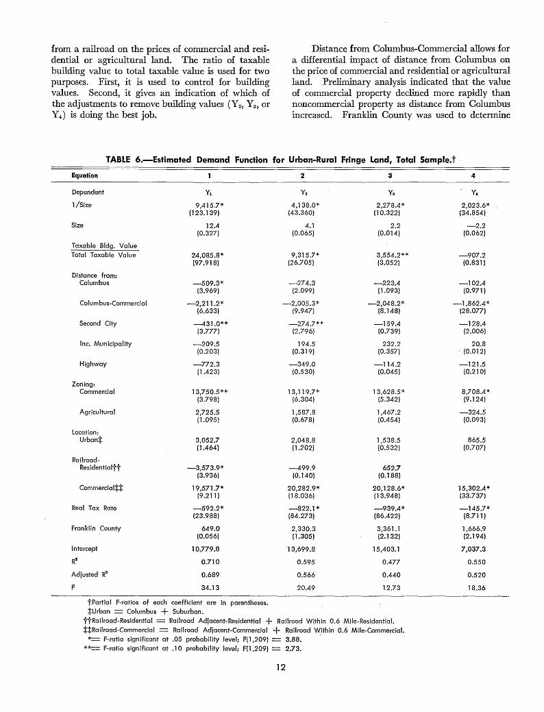
from a railroad on the prices of commercial and resi­dential or agricultural land. The ratio of taxable building value to total taxable value is used for two purposes. First, it is used to control for building values. Second, it gives an indication of which of the adjustments to remove building values (Y2, Ys, or Y4) is doing the best job.

Distance from Columbus-Commercial allows for a differential impact of distance from Columbus on the price of commercial and residential or agricultural land. Preliminary analysis indicated that the value of commercial property declined more rapidly than noncommercial property as distance from Columbus increased. Franklin County was used to determine

TABLE 6.-Estimated Demand Function for Urban-Rural Fringe Land, Total Sample.t

Equation

Dependent Y1

1/Size 9,415.7* (123.139)

Size 12.4 (0.327)

Taxable Bldg. Value Total Taxable Value 24,085.8*

(97.918)

Distance from: Columbus -509.3*

(3.969)

Columbus-Commercia I -2,211.2* (6.633)

Second City -431.0** (3.777)

Inc. Municipality -209.5 (0.203)

Highway -772.3 (l .423)

Zoning: Commercial 13,750.5**

(3.798)

Agricultural 2,725.5 (1.095)

Location: Urban:j: 3,052.7

(1.464)

Railroad-Residentialtt -3,573.9*

(3.936)

Commercial:f::j: 19,571.7* (9.211)

Real Tax Rate -592.2* (23.988)

Franklin County 649.0 (0.056)

Intercept 10,779.8

Ri 0.710

Adjusted R2 0.689

F 34.13

tPartial F-ratios of each coefficient are in parentheses. :j:Urban == Columbus + Suburban.

2 3

Y2 Ya

4,138.0* 2,278.4* (43.360) (10.322)

4.1 2.2 (0.065) (0.014)

9,315.7* 3,554.2** (26.705) (3.052)

-274.3 -223.4 (2.099) (1.093)

-2,005.3* -2,048.2* (9.947] (8.148)

-274.7** -159.4 (2.796) (0.739)

194.5 232.2 (0.319) (0.357)

-349.0 -114.2 (0.530) (0.045)

13,119.7* 13,628.5* (6.304) (5.342)

1,587.8 1,467.2 (0.678) (0.454)

2,048.8 1,538.5 (1.202) (0.532)

-499.9 652.7 (0.140) (0.188)

20,282.9* 20,128.6* (18.036) (13.948)

-822.1* -939.4* (84.273) (86.422)

2,330.3 3,361. l (l.305) (2.132)

13,699.8 15,403.1

0.595 0.477

0.566 0.440

20.49 12.73

ttRailroad-Residential == Railroad Adjacent-Residential + Railroad Within 0.6 Mile-Residential. :f::f:Railroad-Commercial == Railroad Adjacent-Commercial + Railroad Within 0.6 Mile-Commercial.

*== F-ratio significant at .05 probability level; F(l ,209) = 3.88. **= F-ratio significant at .10 probability level; F(l ,209) == 2.73.

12

4

y,

2,023.6* (34.854)

-2.2 (0.062)

-907.2 (0.831)

-102.4 (0.971)

-1,862.4* (28.077)

-128.4 (2.006)

20.8 . (0.012)

-121.5 (0.210)

8,708.4* (9.124)

-324.5 (0.093)

865.5 (0.707)

15,302.4* (33.737)

-145.7* (8.711)

1,666.9 (2.194)

7,037.3

0.550

0.520

18.36

if there was a significant difference between Franklin County and the other counties not explained by the other variables.

Under the assumption that size and characteris­tics of land offered for sale are predetermined to po­tential buyers of land, the relationship can· be esti­mated by ordinary least squares. A further needed assumption is that the left out characteristics (X), which are part of the random component ( e), are un­correlated with the zj. Estimated Results for Total Sample

The total sample results for each dependent vari­able are. presented in Table 6. The equations pre­sented include all factors used in the analysis which had sufficient significance to enter the regression equations. Only these results are presented because the coefficients and standard errors of those variables with F-ratios greater than one generally changed by less than 10% when the other variables were in the equations as compared to when they were not in the equations. Further, equations estimated using sub­samples of the observations were generally consistent with those presented. The F·-ratios of all equations are significant at the 1 % level. Equations 1 and 4 in Table 6 are stressed in the analysis, equation 1 be­cause its dependent variable is actual price per acre and equation 4 because Y4 makes the best adjustment for the removal of building values as evidenced by the insignificant coefficient of Taxable Building Value/ Total Taxable Value.

In Table 6, the coefficients of 1/Size are signifi­cant, while those of Size are not. The partial effects on average price per acre, when the net effect of all other characteristics is set eq~al to zero, from equa­tions 1 and 4 in Table 6 are:

Y1 = 9,415.7 l/Size + 12.4 Size7 (3a} Y4 = 2,023.6 l /Size - 2.2 Size (3b}

Based on this part of the equation, the partial impact of size on land prices is:

Size = 0.5 Y1 = $18,837.6 Y4 = $4,046. l Size = l.0 Y1 = 9,428. l Y4 = 2,021.4 Size = 2.0 Y1 = 4,732.7 Y4 = 1,007.4 Size= 5.0 Y1 = 1,945.1 Y4 = 393.7 Size = 10.0 Y1 = 1,065.6 Y4 = 180.4

The major impact is on the relatively small par­cels of land. The price per acre continues to decline until parcel size reaches about 27 acres in equation 3a. It does not reach a minimum, but declines con­tinuously in equation 3b. These estimates support

7The relatively large coefficient of 1 /Size in equation 1 of Table 6 may be due to a correlation between parcel size and building values which is not removed by Taxable Building Value/Total Taxable Value. Interaction variables between Size and Taxable Building Value/Total Taxable Value were tried, but were not significant and had little impact on the coefficient of 1 /Size.

13

the hypothesis that a potential buyer of land is in search of a parcel of sufficient size to meet his needs and will pay less per unit for a larger parcel of land. An alternative but related interpretation is that the coefficient of 1/Size is a residual value which repre­sents costs such as subdivision costs.

Taxable Building Value/Total Taxable Value is used to control for the impact of buildings on the price of land. Its coefficient is significant in equa­tion 1 of Table 6 with a value of $24,086. In equa­tions 2 and 3, its coefficient is also significant, indica­ting that neither Y2 nor Ya are very effective in adjust­ing for building values. However, Y4 makes a better adjustment for building value since the coefficient of Taxable Building Value/Total Taxable Value is in­significant in equation 4.

The Distance from Columbus and Second City variables show that value of property declines with increasing distance from urban centers. The partial relationship for the decline in price as distance from Columbus increases from equation 1 in Table 6 is:

a Y1 / iJ Distance from Columbus = - 509 .3 - 2211.2 Commercial (4)

If the property is residential or agricultural, each additional mile from Columbus reduces price per acre by an estimated $509. If the property is zoned com­mercial, its value declines by an additional $2,211, or a total of $2, 720 per additional mile from Colum­bus. The additional decline for commercial property is estimated by the coefficient of Distance from Co­lumbus·-Commercial, and is of the same magnitude, negative, and significant in all equations. The co­efficients of Distance from Columbus remain nega­tive for the other three equations, but decline in mag­nitude and significance.

The coefficient of Distance from Second City shows a decline of $431 per acre as the property gets farther from a second city in equation 1 of Table 6. The coefficients remain negative in the other equa­tions, but are of lower magnitude and significance. These results support the hypothesis that distance from urban centers is negatively related to price per acre.

The Distance from Incorporated Municipality coefficient is negative in equation 1, but positive in the other three equations, and insignificant in all equations. Most municipalities in the study area, other than Columbus and the Second Cities, had populations of less than 2,500. Small municipalities generally have little to offer in the way of jobs or shopping centers, and are expected to have a smaller effect on land prices than the metropolitan center or the large incorporated centers. In addition, the two otlier distance measures in the equations may have

picked up part of the effect of the nearest municipal­ity. The simple correlation of Distance from Incor­porated Municipality with Distance from Columbus was 0.25, and with Distance from Second City was 0.26.

The coefficients of these distance variables are algebraically additive. If Distance from Columbus, Second City, and Incorporated Municipality all in­crease by 1 mile, then from equation 1 in Table 6 the price of residential property is expected to decline by $1,150 per acre (-509 -431 -210). However, an increase in Distance from Columbus may be ac­companied by a decrease in Distance from Second City or Incorporated Municipality. For example, if Distance from Columbus increases by 1 mile, but there is a corresponding decrease of 1 mile for both Distance from Second City and Incorporated Munici­pality, then the expected price of residential property increases by $132 per acre (-509 +432 +210).

Preliminary analysis indicated little difference between the value of land located in Columbus and land located in secondary urban centers as compared to unincorporated township land. In Table 6, these two variables are combined to form Urban, a dummy variable equal to one when land is Columbus or sub­urban, zero otherwise. In equation 1 of Table 6, land located in urban centers is $3,053 more valuable than land located in the townships. This result is expected because of the services provided by incorpo­rated areas. The coefficients of Urban in equations 2 to 4 are positive, but of lower magnitude and sig­nificance.

Distance from Highway consistently has a nega­tive sign, but has an F-ratio greater than one only in equation 1 of Table 6. In equation 1, the variable shows that value per acre decreases by $772 for each additional mile a property is located from a major highway.

Preliminary results indicated that land adjacent to a railroad was of approximately equal value to land within 0.6 mile for both commercial and non­commercial property. Although unexpected, this re­sult may be due to a lack of observations where direct access to a railroad was important. Based on the preliminary results, the equations in Table 6 con­tain two railroad variables: Railroad-Residential is equal to one for all residential and agricultural land, including adjacent, within 0.6 mile of a railroad, and zero otherwise; Railroad-Commercial is equal to one for all commercial land, including adjacent, within 0.6 mile of a railroad, and zero otherwise.

Equation 1 of Table 6 shows that residential or agricultural land located within 0.6 mile of a railroad is $3,574 per acre lower in value than such land beyond 0.6 mile. Commercial land within 0.6 mile of

14

a railroad is $19,572 more valuable than commercial land located beyond 0.6 mile from a railroad. The coefficients of Railroad-Residential are insignificant in the last three equations in Table 6, while those of Railroad-Commercial stay positive and significant. One explanation of these results is that the potential for agricultural or residential property near a rail­road moving to commercial use offsets its disadvan­tages for residential use as fong as the property is not committed to residential use, i.e., as long as residen­tial housing values are not considered. However, commitment to residential use causes the value of this property to decline relative to residentially committed property where railroads are not a factor, although the absolute value of the property may still increase.

The Commercial zoning coefficient of $13, 750 per acre in equation 1 of Table 6 is the estimated value of commercial land above residential land in Columbus and more than 0.6 mile from a railroad. For other commercial land, Distance from Columbus­Commercial and Railroad-Commercial must also be considered. For each additional mile commercial property is located from Columbus, its value de­creases by $2,720 per acre. If the commercial prop­erty is within 0.6 mile of a railroad, its value in­creases by $19,572. The Commercial variable is sig­nificant in all equations and its coefficient changes little, especially in the first three equations.

The positive coefficients of agricultural land in equations 1 to 3 of Table 6 are unexpected. Resi­dential land is expected to be more valuable than agricultural land. There are two possible reasons for the positive values. First, the agricultural land observations may consist largely of small farms with relatively large building values bought as hobby farms by city residents. The negative coefficient of equa­tion 4 is consistent with this explanation. Second, the land may have been purchased for speculative purposes but kept in agricultural use.

The coefficients of the Real Tax Rate are nega­tive and significant in all equations. Equation 1 shows that an increase of 1 mill in the tax rate, about 10% from the mean Real Tax Rate in the sample, decreases value of property by an estimated $592 per acre. Complete removal of the property tax at the mean would increase price per acre by about $6,870. The corresponding changes from equation 4 are a decrease of $146 per 1-mill increase in the Real Tax Rate and an increase of $1,690 with complete re­moval of the property tax at its mean level. A 1-mill increase in Real Tax Rate is equivalent to about 4 mills in the actual property tax rate.

The coefficients of Franklin County in Table 6 show that land in Franklin County is more valuable than land outside of Franklin County. This variable

was included as a control for institutional structure differences between the urban Franklin County and the rural surrounding counties. The relatively great­er magnitude and significance of the coefficients in equations 2 to 4 indicate that the major structural differences affecting land prices may be in the ap­praisal and assessment of property values for property tax purposes.

Estimated Results for Franklin County Table 7 presents four equations using the 65 ob­

servations from the sample in Franklin County. Table 8 presents three equations using 59 observations

of 1971 sales in Franklin County. These 59 observa­tions were initially used in the development and test­ing of a preliminary version of the demand model for this study. All equations have significant F-ratios at the 1 % probability level.

Generally, the Franklin County results in Table 7 are similar in magnitude and sign to the total sample results in Table 6. Many of the differences, particularly in the magnitudes of coefficients, can be attributed to the restriction of the sample to Franklin County. The results for 1/Size, Size, the railroad variables, the zoning variables, Distance from Co-

TABLE 7.-Estimated Demand Functions for Urban-Rural Fringe Land, Franklin County, 1972.t

Equation

Dependent

l/Size

Size

Taxable Bldg. Value

Total Taxable Value

Distance from: Columbus

Columbus-Commercial

Highway

Zoning: Commercial

Agricultural

Location: Columbus

Suburban

Railroad: Residential:j:

Commercialtt

Rea I Tax Rate

Intercept

R2

Adjusted R2

F

14,309.l* (70.521)

11.7 (0.037)

30,819.0* (30.512)

-777.l (0.629)

-4,816.3 (2.456)

33,939.3** (3.785)

11,671.0 {l .753)

l,584.9 (0.137)

6,812.3 {l .784)

-6,192.3 (2.781 J

5,668.6 (0.206)

-602.7* (5.700)

-211.7

0.795

0.748

16.84

tPartial F-ratios of each coefficient are in parentheses.

2

5,885.2* (19.498)

7,092.l (2.784)

-786.6 {l.120)

-5,155.8* (4.907)

800.3 (0.464)

28,677.8* (4.584)

2,609.3 (0.213)

4,636.2 {l .464)

-2,617.4 (0.850)

8,469.3 (0.782)

-537.9* (7.860)

l 0,258.7

0.643

0.568

8.66

3

Ya

2,896.0* (4.627)

-8.8 (0.050)

-1,463.7 (0.119)

-804.l (1.060)

-5,285.l * (4.843)

l,170.6 (0.946)

27,002.4** (3.859)

-952.8 (0.079)

3,748.5 (0.870)

-1,337.4 (0.211)

9,521.5 0.943)

-523.3* (7.038)

14,149.3

0.541

0.435

5.11

:j:Railroad-Residential == Railroad Adjacent-Residential + Railroad Within 0.6 Mile-Residential. ttRailroad-Commercial == Railroad Adjacent-Commercial + Railroad Within 0.6 Mile-Commercial.

*==F-ratio significant at .05 probability level; F{l ,51) == 4.03. * *==F-ratio significant at .1 0 probability level; F{l ,51) == 2 .81.

15

4

3,682.5* (10.543)

-4.3 (0.011)

-7,283.8** (3.805)

-565.5 (0.732)

-2,853.1 (l.943)

l.174.l (l.301)

13,187.5 (l .290)

-1,943.4 (0.108)

-964.7 (0.112)

2,510.6 (0.543)

13,234.6 (2.512)

-233.3 (l.881)

9,985.l

0.520

0.409

4.70

lumbus-Commercial, and the Real Tax Rate are simi­lar. Differences exist with respect to Taxable Build­ing Value/Total Taxable Value, Distance from Co­lumbus, the location variables, and Distance from Highway.

The negative and significant coefficient of Tax­able Building Value/Total Taxable Value in equa­tion 4 of Table 7 indicates that Y4 overadjusts for building values. Equation 3 with a small insignifi~

TABLE 8.-Estimated Demand Functions for Ur­ban-Rural Fringe Land, Franklin County, 1971. t Equation

Dependent

l/Size

Size

Taxable Bldg. Value

Total Taxable Value

Distance fwm: Columbus

Columbus­Commercial

Highway

Zoning: Commercial

Agricultural

Location: Columbus

Suburban.

Railroad: Adjacent­Residential

Within 0.6 Mile­Residential

Adjacent­Commercial

Within 0.6 Mile­Commercial

Rea I Tax Rate:j:

Intercept

R2

Adjusted R2

F

18,853.3* (27.038)

333.5 (2,404)

24,669.6* (9.041)

-365.0 (0.059)

-1,430.7 (0.282)

2

13,021.4* (20.491)

105.8 (0.406)

-651.2 (0.301)

-2,094.4 (0.930)

-4,703.4** -3,312.9 (3.490) (2.652)

19,290.9 (2.500)

4,837.4 (0.144)

16,827.9* (4.854)

1,241.4

14,947.l (l.151)

17,373.5** (3.100)

4,096.5 (0.165)

14,343.6* (5.399)

5,469.2

14,905.8 (l.755)

3

y4.

11,922.3* (18.890)

49.5 (0.092)

-11,316.8** (3.324)

-370.7 (0.106)

-1,552.8 (0.580)

-2,417.2 (l.610)

13,224.3 (2.052)

1,889.6 (0.038)

12,694.4* (4.825)

3,781.0

13,182.7 (l.564)

-16,884.2 -16,965.7** -16,977. l ** (l.874) (2.907) (3.310)

5,774.2 (0.255)

-11,622.5 (1.386)

242.8 (l.325)

-10,503.7

0.635

0.508

4.99

-6,677.4 (0.524)

-3,715.2 (0.218)

141.5 (0.688)

972.4

0.615

0.493

5.03

-9,224.4 (l.139)

-2,479.3 (0.110)

171.8 (l.159)

2,850.7

0.613

0.478

4.54

tPartial F-ratios of each coefficient are in parentheses. :j:Real Tax Rate == actual property tax/total sales value. *== F-ratio significant at .05 probability level; F(l ,43) == 4.06.

**== F-ratio significant at .10 probability level; F(l ,43) == 2.83.

16

cant coefficient is probably the best alternative esti­mate to equation 1 of the Franklin County demand for land net of building values. For the total sample, Y4 made the best adjustment to remove building values.

The results for Distance from Columbus in Table 7 are consistent with the combined impact of Distance from Columbus, Second City, and Incorporated Municipality in the equations of Table 6. Only Dis­tance from Columbus is used in the Franklin County sample because of the restricted geographical limits of the sample.

In the Franklin County sample, the coefficients of location in Columbus or Suburban indicated that these variables could not be combined as they were in the· total sample. The results in Table 7 indicate that land in Columbus is of approximately equal value to land in unincorporated areas when other characteristics are taken into consideration, while suburban land is of greater value.

The Distance from Highway coefficients are positive in Table 7 in contrast to the expected nega­tive coefficients in the equations of Table 6. How­ever, none of the coefficients are significantly differ­ent from zero at the .10 probability level. An in­crease in distance from an urban access highway is expected to increase the transportation and time costs of reaching the parcel.

Differences also exist between the 1972 and 1971 Franklin County results. The results in Table 8 are similar to those of Table 7 with respect to 1/Size, Size, Distance from Columbus, Distance from Columbus­Commercial, and the zoning variables. They differ with respect to Taxable Building Value/Total Tax­able Value, the location variables, Distance from Highway, the railroad variables, and the Real Tax · Rate.

Based on the coefficients of Taxable Building Value/Total Taxable Value in Table 8, variable Y2

makes the best adjustment for building values in the 1971 Franklin County sample. Variable Y3 is not available. As in the 1972 results, Y4 overadjusted for building values.

The 1971 results for location in Columbus indi­cate a significantly greater value than the 1972 re­sults. In Table 8, the estimates show that land lo­cated in Columbus is $10,118 to $15,253 more valu­able than land located in the unincorporated town­ships. In 1972, these two locations were of approxi­mately equal value. Except for equation 1 in Table 8, the coefficients of Suburban location are similar for the 2 years.

The coefficients of Distance from Highway are negative and of relatively large magnitude in all three equations of Table 8. In contrast, Distance from

Highway yielded positive coefficients in the equations of Table 7. In the total sample, the coefficients were negative but of smaller magnitude than those in Table 8.

The results for the railroad variables in Table 8 indicate that all four of the variables are needed. Railroad within 0.6 Mile-Residential yields expected negative coefficients, but they are large at about $17,000. The large positive coefficients of residen­tial and agricultural property adjacent to railroads indicate that the observations in the sample had high probabilities of being zoned for commercial use.

The impact of railroads on commercial property in Table 8 is generally negative, in contrast to the results in Tables 6 and 7. The coefficients are not significant but are affected by adjustments for build­ing values.

In Table 8, the Real Tax Rate uses actual prop­erty taxes paid in 1971, in contrast to property tax rate times taxable value used for the 1972 sample. Conceptually, these definitions are identical. The coefficients of the Real Tax Rate are positive, but in­significant at the .10 probability level in Table 8, in contrast to negative significant coefficients for the

total sample and the 1972 Franklin County sample. The means and ranges of Real Tax Rate .are similar in all samples. However, the standard deviation for the 1971 sample is twice as large as the standard de­viation of Real Tax Rate for the 1972 samples, total and Franklin County. One explanation of the con­trasting results and the change in standard deviation of real tax rate between 1971 and 1972 is that several Ohio Supreme Court rulings on property tax issues and the 35% assessment rule have caused property assessments to reflect property values more accurate­ly. For example, procedures for implementing the 35 % assessment rule were formulated and being im­plemented in 1972, but not in 1971.

The results of the total sample and the two Franklin County samples are generally consistent. In particular, the estimated equations for the total and 1972 Franklin County samples differ in ways largely explainable by the .change in sample area. The cliff erences in the 1971 Franklin County esti­mates are probably caused by changes in property tax assessment practices and by characteristics such as topography or railroad access which are not suffi­ciently controlled in the equations.

CONCLUSIONS AND IMPLICATIONS

This study uses 225 observations of undeveloped land within a 25-mile radius of Columbus, Ohio, dur­ing 1972 to estimate the urban demand for land in the urban-rural fringe. Further results were pre­sented for the 65 observations in 1972 and an addi­tional 59 observations for 1971 from Franklin Coun­ty, in which Columbus is located. This section iso­lates the major conclusions, policy implications, and further research needs implied by this study.

Conclusions Caution needs to be exercised in the interpreta-

tion of the results for two reasons. First, the scope of the study is limited to a relatively small number of observations and to a single urban center. Second, the ability to control for the impact of buildings on land prices is limited. The impact of buildings is controlled through the removal of building values from price per acre under alternative assumptions about property tax assessment values and through the inclusion of the ratio of taxable building value to total taxable value as a variable in the regression equations. These adjustments yield results which are generally consistent in sign and statistical signific­ance, but the magnitudes of the coefficients often de­cline with increased adjustments for building values. It is not possible to determine whether these changes are due to interactions between the land parcels and

17

buildings not controlled in the equations or inappro­priate adjustments for building values.

The results show that per acre land values de­cline with increasing size of parcel, and that the rate of decline is rapid for small-size parcels. The results are consistent with the hypothesis that land buyers seek parcels of sufficient minimum size for their needs, and will pay little for additional size. They are also consistent with the related hypothesis that a land par­cel has a residual value independent of size, which is related to subdivision costs, i.e., the costs of creating a new land parcel.

Residential land values decline by $200 to $1,150 per acre for each additional mile from an ur­ban center. Of this total, $100 to $600 can be at­tributed to distance from Columbus and the remain­der to secondary urban centers. The value of com­mercial property declines more rapidly than residen­tial property. The estimates indicate that commer­cial property declines by $1,500 to $2,200 per acre more rapidly than residential property per increase of 1 mile in distance from Columbus, or as much as $2,800 per acre in total.

In the total sample, land located in Columbus and the incorporated suburbs is $860 to $3,000 per acre more valuable than land located in the unin­corporated townships. However, none of the coef­ficients are significant at the .10 probability level.

The results from the 1972 Franklin County sample indicate that land located in the suburbs is of greater value than that in Columbus or the townships. The 1971 Franklin County sample shows a similar rela­tionship between the suburbs and townships, but it shows that land in Columbus is of greater value than land located in either the suburbs or townships.

The distance from an urban access highway has a negative effect on land values in the total sample, but none of the coefficients are significant at the .10 probability level. In the .. 1971 Franklin County sample, the impact is also negative, but distance from a highway has positive coefficients in the 1972 Frank­lin County sample. There are two possible reasons for these results. First, for property located several miles from an urban center, the importance of dis­tance from the property to an urban access highway may be small relative to the total distance to the ur­ban center. Second, most observations in the samples were relatively close to urban access highways, and this may not be an important characteristic for the samples. The average distance from a highway in the total 1972 sample was only 1.22 miles, with a maximum distance of 7 miles, and an average of 1 mile, with a maximum of 5 miles for the 1971 Frank­lin County sample.

The coefficients of the railroad variables for the total sample indicate that residential or agricultural land within 0.6 mile of a railroad is $650 more valu­able to $3,500 less valuable per acre than similar land located beyond 0.6 mile of a railroad. Commercial land within 0. 6 mile of a railroad is $15, 000 to $20,000 per acre more valuable than commercial land beyond 0.6 mile. The 1972 Franklin County results support these conclusions, but the 1971 re­sults do not. However, the 1971 results may be due to expected· zoning changes on noncommercial prop­erty adjacent to railroads and undesirable charac­teristics of commercial property near railroads not included in the equations.

Land zoned commercial is about $13,500 more valuable per acre than land zoned for other uses in Columbus. However, the value of commercial land declines rapidly with increasing distance from Co­lumbus. Its value is also sensitive to railroad access.

The results generally indicate that land used for agricultural purposes is more valuable than residen­tial land. This unexpected result is probably due to a special aspect of the urban-rural fringe where agricultural land is purchased for hobby farms or for speculative purposes.

The property tax has a negative, significant, and larger than expected impact on land values. A 1-mill increase in the real property tax rate (about 10%) decreases land values per acre by an estimated

18

$146 to $592 .. A 1-mill increase in the real property tax rate is equivalent to about 4 mills in the nominal or actual property tax rate at the sample means of 11.6 and 45.5 mills, respectively, for these two mea­sures of the property tax rate.

Policy Implications The factors in th~s study under the direct con-

trol of the community are zoning and the property tax. Three implications of this study for zoning and property tax policy are:

9 Communities which have large lot zoning policies should compare the advantages of such zoning to the costs it imposes on individual landowners and on the community. The results of this study show that land prices per acre decline rapidly with in­creasing parcel size for small land parcels. For ex­ample, the value of two one-half acre parcels could exceed the value of a 1-acre parcel by more than $9,000. Minimum residential housing lot size re­strictions of 1 acre or more per lot impose large costs on owners of undeveloped land through reduced property values. In addition, there are costs to the community, such as reduced tax base per acre of land and increased costs of extending roads, water and sewer systems, and police and fire protection to a more dispersed population. These costs should be compared to the benefits of large lot zoning policies, such as fewer people and smaller demands on the school system.

• Land use zoning policies can generate large economic values on property zoned for commercial use. In this study, these values exceed $30,000 per acre on some land parcels. Owners of land well lo­cated for commercial development can be expected to incur large costs to obtain zoning for commercial development. Community officials are attracted to the increased property tax base provided by commer­cial development. Under current land use zoning policies, urban development plans can be expected to have relatively little influence, even with strong community support, in the face of pressures from large landowners and public officials with a short­time horizon when zoning decisions are made.

If land use control polices are to be less subject to private landowner and short-run political pres·­sures, they should be designed to reduce or eliminate the private market values which present zoning poli­cies generate. Two possible directions for policy to reduce these market values are to increase the supply of commercial property and/ or to design taxation­compensation policies or new definitions of property rights which reduce the windfall gains to and losses imposed on landowners from zoning decisions.

• The results of this study show a negative and significant impact of property tax rates on land prices. However, this impact is small when com­pared to other factors, such as zoning. A 10% in­crease in the real property tax rate would decrease land prices by less than $600 per acre. The property tax probably has a greater impact on land use. In particular, the tax on buildings and improvements provides an incentive to move land from agriculture or other low intensity uses into idle land. It may discourage renovation or upgrading of buildings. In­creasing taxes on land itself, although making agricul­tural use unprofitable in the long run, will not neces­sarily drive land out of agriculture in the short run if improvements are not taxed. Such a tax on land only (i.e., a site value tax) could be part of a taxa­tion-compensation policy for the implementation of community land use objectives.

Issues for Further Study

• The portion of the property tax which is on buildings and other improvements provides an incen­tive. to reduce the extent of improvements on proper­ty. This incentive is expected to increase with in­creasing property tax rates. However, little is known about the magnitude of the effect, in particular its role in moving land out of agriculture or low intensity urban uses into idle land while in trGi:nsition to high intensity urban uses. A study of the relationship be­tween property tax rates and land use would provide valuable information to determine by how much idle land would decline with reduction or removal of the property tax on improvements.

• The role of buildings in land price determi­nation has not been fully controlled in this study. Although separate demand functions for land were estimated from the observations which did not have buildings in the sample, these estimates did not sup­port one method of control over others. A more ex­tensive study of transactions of land which have no buildings would provide further needed information on the demand for undeveloped land. This infor­mation is needed for the development of land use policies and for more complete evaluation of the im­pact on land use of changes in the property tax structure.

• Several factors not included in this study probably account for the inconsistencies in the re­sults. Topography, trees, and other environmental factors affect the appearance of land sites to potential homeowners and the development costs to prepare the land for construction. Deferred payment or sell­er-financed contracts, which could not be isolated from information available for this study, may affect not only prices, but the dates on which transactions

19

are recorded. Future studies of the demand for and use of land should incorporate these factors when re­sources permit. However, incorporation of these factors is likely to require on-site inspection for each observation and interviews with persons who have direct knowledge of each transaction, and therefore will require significantly larger resource outlays than available for this study.

• This study has found that zoning has large and significant impacts on land prices. However, zoning is only one of several control measures (such as subdivision regulations, building codes, and health codes) which communities can use in the implemen­tation of land use plans. Further study of the feasi­bility of using various control policies to implement land use plans and to control market forces is needed.

• Most studies of urban-rural fringe land values, including this study, are limited to single ur­ban centers during relatively short time periods. A longer run objective of this research should be to de­velop both interurban and longitudinal studies so that the demand for land can be compared betvyeen urban centers and over time. This research is needed for the development and implementation of land use policies at the state and national levels.

LITERATURE CITED l. Armbrister, Trevor. July 1973. Surprises from

the 1970 Census. Reader's. Digest, pp. 135-139. 2. Clawson, Marion. 1972. America's Land and

Its Uses. Resources for the Future, Inc., Johns Hopkins Press, Baltimore.

3. Clonts, Howard A. Jr. Nov. 1970. Influences of Urbanization on Land Values at the Urban Peri­phery. Land Econ., 46: 489-497.

4. Downing, Paul B. Feb. 1973. Factors Affecting Commercial Land Values: An Empirical Study of Milwaukee, Wisconsin. Land Econ., 49: 44-56.

5. Halcrow, Harold G., et al. 1973. School Tax Op­tions Affecting Illinois Agriculture. Univ. of Ill. Agri. Exp. Sta., Bull. 7 44.

6. Hammill, Anne E. April 1969. Variables Related to Farm Real Estate Values ,in Minnesota Coun­ties. Agri. Econ. Res., 21 :45-50.

7. Kinney, Robert R. Feb. 1973. A Summary of Information in Regard to Equalization of Real Property Tax Values in Ohio for 1972 Tax Year. Board of Tax Appeals, State of Ohio, Columbus, No. 757-A.

8. Paseur, E. C. 1973. Real Property Taxes and Farm Real Estate Values in North Carolina. Econ. Res. Report 25, Dept. of Economics, North Caro­lina State Univ.

9. Schuh, G. Edward and Wesley C. Scharlach. Nov. 1966. Qualitative Analysis of Some Farm and Non-Farm Determinants of Agricultural Land Values-Impact of Economic Development. Pur­due Agri. Exp. Sta., Bull. 821.

l 0. The 1972 World Almanac. 1971. Newspaper En­terprise Association, Inc., New York, Cleveland.

BETTER LIVl·NG IS THE PRODUCT of research at the Ohio Agricultural Research and Development Center. All Ohioans benefit from this product.

Ohio's 110,000 farm families benefit from the results of agr.icul·· tural research translated into increased earnings and improved living conditions. So do the families of the thousands of workers employed in the firms making up the state's $8 billion agribusiness complex.

But the greatest benefits of agricultural research flow to the mil­lions of Ohio consumers. They enjoy the end products of agricultural science-the world's most wholesome and nutritious food, attractive lawns, beautiful ornamental plants, and hundreds of consumer prod­ucts containing ingredients originating on the farm, in the greenhouse and nursery, or in the forest.

The Ohio Agricultural Experiment Station, as the Center was called for 83 years, was established at The Ohio State University, Columbus, in 1882. Ten years later, the Station was moved to its present loca­tion in Wayne County. In 1965, the Ohio General Assembly passed legislation changing the name to Ohio Agricultural Research and De­velopment Center-a name which more accurately reflects the nature and scope of the Center's research program today.

Research at OARDC deals with the improvement of all agricul­tural production ·and marketing practices. It is concerned with the de­velopment of an agricultural product from germination of a seed or development of an embryo through· to the consumer's dinner table. It is directed at improved human nutrition, family and child development, home management, and all other aspects of family life. It is geared to enhancing and preserving the quality of our environment.

lndivi~uals and groups are welcome to visit the OARDC, to enjoy the attractive buildings, grounds, and arboretum, and to observe first hand research aimed at the goal of Better Living for All Ohioans!