The Delta Parallel Robot: Kinematics Solutions Robert L. Williams II, Ph.D., williar4@ohio.edu

Mechanical Engineering, Ohio University, April 2015

Clavel’s Delta Robot1 is arguably the most successful commercial parallel robot to date. The left image below shows the original design from Clavel’s U.S. patent2, and the right photograph below shows one commercial instantiation of the Delta Robot.

Delta Robot Design1 ABB FlexPicker Delta Robot

www.abb.com

The Delta Robot has 4-degrees-of-freedom (dof), 3-dof for XYZ translation, plus a fourth inner leg to control a single rotational freedom at the end-effector platform (about the axis perpendicular to the platform). The remainder of this document will focus only on the 3-dof XYZ translation-only Delta Robot since that is being widely applied by 3D printers and Arduino hobbyists.

Presented is a description of the 3-dof Delta Robot, followed by kinematics analysis including

analytical solutions for the inverse position kinematics problem and the forward position kinematics problem, and then examples for both, snapshots and trajectories. The velocity equations are also derived This is presented for both revolute-input and prismatic-input Delta Robots. For referencing this document, please use:

R.L. Williams II, “The Delta Parallel Robot: Kinematics Solutions”, Internet Publication, www.ohio.edu/people/williar4/html/pdf/DeltaKin.pdf, April 2015.

1 R. Clavel, 1991, “Conception d'un robot parallèle rapide à 4 degrés de liberté”, Ph.D. Thesis, EPFL, Lausanne, Switzerland. 2 R. Clavel, 1990, “Device for the Movement and Positioning of an Element in Space”, U.S. Patent No. 4,976,582.

2

Table of Contents

REVOLUTE-INPUT DELTA ROBOT ................................................................................................... 3

REVOLUTE-INPUT DELTA ROBOT DESCRIPTION ........................................................................................ 3 REVOLUTE-INPUT DELTA ROBOT MOBILITY ............................................................................................. 7 PRACTICAL REVOLUTE-INPUT DELTA ROBOTS ......................................................................................... 9 REVOLUTE-INPUT DELTA ROBOT KINEMATICS ANALYSIS ....................................................................... 10

Inverse Position Kinematics (IPK) Solution ....................................................................................... 11 Forward Position Kinematics (FPK) Solution ................................................................................... 12 Revolute-Input Delta Robot Velocity Kinematics Equations .............................................................. 15

REVOLUTE-INPUT DELTA ROBOT POSITION KINEMATICS EXAMPLES ...................................................... 16 Inverse Position Kinematics Examples .............................................................................................. 16 Forward Position Kinematics Examples ............................................................................................ 19

PRISMATIC-INPUT DELTA ROBOT ................................................................................................. 22

PRISMATIC-INPUT DELTA ROBOT DESCRIPTION ...................................................................................... 22 PRACTICAL PRISMATIC-INPUT DELTA ROBOTS ........................................................................................ 25 PRISMATIC-INPUT DELTA ROBOT KINEMATICS ANALYSIS ....................................................................... 26

Inverse Position Kinematics (IPK) Solution ...................................................................................... 27 Forward Position Kinematics (FPK) Solution ................................................................................... 29 Prismatic-Input Delta Robot Velocity Kinematics Equations ............................................................ 33

PRISMATIC-INPUT DELTA ROBOT POSITION KINEMATICS EXAMPLES ...................................................... 34 Inverse Position Kinematics Examples .............................................................................................. 34 Forward Position Kinematics Examples ............................................................................................ 37

ACKNOWLEDGEMENTS ................................................................................................................... 40

APPENDICES ......................................................................................................................................... 41

APPENDIX A. THREE-SPHERES INTERSECTION ALGORITHM ................................................................... 41 Example .............................................................................................................................................. 43 Imaginary Solutions ........................................................................................................................... 43 Singularities ....................................................................................................................................... 43 Multiple Solutions .............................................................................................................................. 44

APPENDIX B. SIMPLIFIED THREE-SPHERES INTERSECTION ALGORITHM ................................................ 45

3

Revolute-Input Delta Robot

Revolute-Input Delta Robot Description As shown below, the 3-dof Delta Robot is composed of three identical RUU legs in parallel

between the top fixed base and the bottom moving end-effector platform. The top revolute joints are actuated (indicated by the underbar) via base-fixed rotational actuators. Their control variables are

, 1,2,3i i about the axes shown. In this model i are measured with the right hand, with zero angle

defined as when the actuated link is in the horizontal plane. The parallelogram 4-bar mechanisms of the three lower links ensure the translation-only motion. The universal (U) joints are implemented using three non-collocated revolute (R) joints (two parallel and one perpendicular, six places) as shown below.

Delta Parallel Robot Diagram

adapted from: elmomc.com/capabilities

4

The three-dof Delta Robot is capable of XYZ translational control of its moving platform within its workspace. Viewing the three identical RUU chains as legs, points , 1,2,3iB i are the hips, points

, 1,2,3iA i are the knees, and points , 1,2,3iP i are the ankles. The side length of the base

equilateral triangle is sB and the side length of the moving platform equilateral triangle is sP. The moving platform equilateral triangle is inverted with respect to the base equilateral triangle as shown, in a constant orientation.

Delta Robot Kinematic Diagram

The fixed base Cartesian reference frame is {B}, whose origin is located in the center of the base

equilateral triangle. The moving platform Cartesian reference frame is {P}, whose origin is located in the center of the platform equilateral triangle. The orientation of {P} is always identical to the

orientation of {B} so rotation matrix 3BP R I is constant. The joint variables are 1 2 3

T Θ , and

the Cartesian variables are TBP x y zP . The design shown has high symmetry, with three upper

leg lengths L and three lower lengths l (the parallelogram four-bar mechanisms major lengths). The Delta Robot fixed base and platform geometric details are shown on the next page.

5

Delta Robot Fixed Base Details

Delta Robot Moving Platform Details

6

The fixed-base revolute joint points iB are constant in the base frame {B} and the platform-fixed

U-joint connection points iP are constant in the base frame {P}:

1

0

0

BBw

B 2

3

21

20

B

BB

w

w

B 3

3

21

20

B

BB

w

w

B

1

0

0

PPu

P 2

2

0

P

PP

s

w

P 3

2

0

P

PP

s

w

P

The vertices of the fixed-based equilateral triangle are:

1

2

0

B

BB

s

w

b 2

0

0

BBu

b 3

2

0

B

BB

s

w

b

where:

3

6B Bw s 3

3B Bu s 3

6P Pw s 3

3P Pu s

name meaning value (mm) sB base equilateral triangle side 567 sP platform equilateral triangle side 76 L upper legs length 524 l lower legs parallelogram length 1244 h lower legs parallelogram width 131 wB planar distance from {0} to near base side 164 uB planar distance from {0} to a base vertex 327 wP planar distance from {P} to near platform side 65 uP planar distance from {P} to a platform vertex 131

The model values above are for a specific commercial delta robot, the ABB FlexPicker IRB 360-1/1600, scaled from a figure (new.abb.com/products). Though Delta Robot symmetry is assumed, the following methods may be adapted to the general case.

7

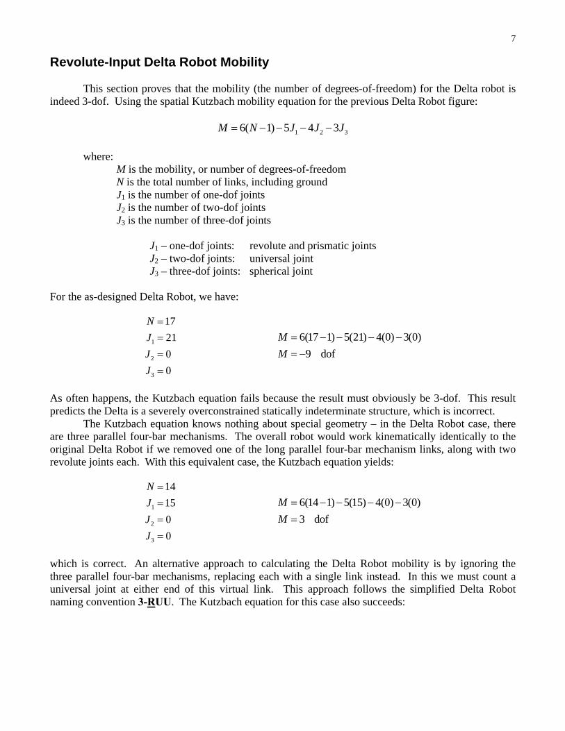
Revolute-Input Delta Robot Mobility

This section proves that the mobility (the number of degrees-of-freedom) for the Delta robot is indeed 3-dof. Using the spatial Kutzbach mobility equation for the previous Delta Robot figure:

1 2 36( 1) 5 4 3M N J J J

where: M is the mobility, or number of degrees-of-freedom N is the total number of links, including ground J1 is the number of one-dof joints J2 is the number of two-dof joints J3 is the number of three-dof joints

J1 – one-dof joints: revolute and prismatic joints J2 – two-dof joints: universal joint J3 – three-dof joints: spherical joint

For the as-designed Delta Robot, we have:

1

2

3

17

21

0

0

N

J

J

J

6(17 1) 5(21) 4(0) 3(0)

9 dof

M

M

As often happens, the Kutzbach equation fails because the result must obviously be 3-dof. This result predicts the Delta is a severely overconstrained statically indeterminate structure, which is incorrect. The Kutzbach equation knows nothing about special geometry – in the Delta Robot case, there are three parallel four-bar mechanisms. The overall robot would work kinematically identically to the original Delta Robot if we removed one of the long parallel four-bar mechanism links, along with two revolute joints each. With this equivalent case, the Kutzbach equation yields:

1

2

3

14

15

0

0

N

J

J

J

6(14 1) 5(15) 4(0) 3(0)

3 dof

M

M

which is correct. An alternative approach to calculating the Delta Robot mobility is by ignoring the three parallel four-bar mechanisms, replacing each with a single link instead. In this we must count a universal joint at either end of this virtual link. This approach follows the simplified Delta Robot naming convention 3-RUU. The Kutzbach equation for this case also succeeds:

8

1

2

3

8

3

6

0

N

J

J

J

6(8 1) 5(3) 4(6) 3(0)

3 dof

M

M

Either of the second two approaches works. The author prefers the former since it is closer to the actual Delta Robot design.

9

Practical Revolute-Input Delta Robots

Delta Chocolate-Handling Robot Delta Pick-and-Place Robots sti.epfl.ch en.wikipedia.org/wiki/Delta_robot

Delta Robot 3D Printer Sketchy Delta Robot en.wikipedia.org/wiki/Delta_robot en.wikipedia.org/wiki/Delta_robot

Novint Falcon Haptic Interface Fanuc Delta Robot images.bit-tech.net robot.fanucamerica.com

10

Revolute-Input Delta Robot Kinematics Analysis From the kinematic diagram above, the following three vector-loop closure equations are written for the Delta Robot:

B B B B B P B Pi i i P P i P i B L l P R P P P 1,2,3i

where 3

BP R I since no rotations are allowed by the Delta Robot.

The three applicable constraints state that the lower leg lengths must have the correct, constant length l (the virtual length through the center of each parallelogram):

B B P B Bi i P i i il l P P B L 1,2,3i

It will be more convenient to square both sides of the constraint equations above to avoid the square-root in the Euclidean norms:

22 2 2 2Bi i ix iy izl l l l l 1,2,3i

Again, the Cartesian variables are TBP x y zP . The constant vector values for points iP

and iB were given previously. The vectors BiL are dependent on the joint variables

1 2 3

T Θ :

1 1

1

0

cos

sin

B L

L

L

2

2 2

2

3cos

21

cos2

sin

B

L

L

L

L

3

3 3

3

3cos

21

cos2

sin

B

L

L

L

L

Substituting all above values into the vector-loop closure equations yields:

1 1

1

cos

sin

B

x

y L a

z L

l

2

2 2

2

3cos

21

cos2

sin

B

x L b

y L c

z L

l

3

3 3

3

3cos

21

cos2

sin

B

x L b

y L c

z L

l

11

where: 3

2 21

2

B P

PB

P B

a w u

sb w

c w w

And the three constraint equations yield the kinematics equations for the Delta Robot:

2 2 2 2 2 21 1

2 2 2 2 2 2 22 2

2 2 2 2 2 2 23 3

2 ( ) cos 2 sin 2 0

( 3( ) ) cos 2 sin 2 2 0

( 3( ) ) cos 2 sin 2 2 0

L y a zL x y z a L ya l

L x b y c zL x y z b c L xb yc l

L x b y c zL x y z b c L xb yc l

The three absolute vector knee points are found using B B Bi i i A B L , 1,2,3i :

1 1

1

0

cos

sin

BBw L

L

A

2

2 2

2

3( cos )

21

( cos )2

sin

B

BB

w L

w L

L

A

3

3 3

3

3( cos )

21

( cos )2

sin

B

BB

w L

w L

L

A

Inverse Position Kinematics (IPK) Solution

The 3-dof Delta Robot inverse position kinematics (IPK) problem is stated: Given the Cartesian

position of the moving platform control point (the origin of {P}), TBP x y zP , calculate the three

required actuated revolute joint angles 1 2 3

T Θ . The IPK solution for parallel robots is often

straightforward; the IPK solution for the Delta Robot is not trivial, but can be found analytically. Referring to the Delta Robot kinematic diagram above, the IPK problem can be solved independently for each of the three RUU legs. Geometrically, each leg IPK solution is the intersection between a known

circle (radius L, centered on the base triangle R joint point BiB ) and a known sphere (radius l, centered

on the moving platform vertex PiP ).

This solution may be done geometrically/trigonometrically. However, we will now accomplish

this IPK solution analytically, using the three constraint equations applied to the vector loop-closure equations (derived previously). The three independent scalar IPK equations are of the form:

cos sin 0i i i i iE F G 1,2,3i

where:

12

1

1

2 2 2 2 2 21

2 ( )

2

2

E L y a

F zL

G x y z a L ya l

2

2

2 2 2 2 2 2 22

( 3( ) )

2

2( )

E L x b y c

F zL

G x y z b c L xb yc l

3

3

2 2 2 2 2 2 23

( 3( ) )

2

2( )

E L x b y c

F zL

G x y z b c L xb yc l

The equation cos sin 0i i i i iE F G appears a lot in robot and mechanism kinematics and is readily

solved using the Tangent Half-Angle Substitution.

If we define tan2

iit

then

2

2

1cos

1i

ii

t

t

and 2

2sin

1i

ii

t

t

Substitute the Tangent Half-Angle Substitution into the EFG equation:

2

2 2

1 20

1 1i i

i i ii i

t tE F G

t t

2 2(1 ) (2 ) (1 ) 0i i i i i iE t F t G t

2( ) (2 ) ( ) 0i i i i i i iG E t F t G E quadratic formula: 1,2

2 2 2i i i i

ii i

F E F Gt

G E

Solve for i by inverting the original Tangent Half-Angle Substitution definition:

12 tan ( )i it

Two i solutions result from the in the quadratic formula. Both are correct since there are two valid

solutions – knee left and knee right. This yields two IPK branch solutions for each leg of the Delta Robot, for a total of 8 possible valid solutions. Generally the one solution with all knees kinked out instead of in will be chosen. Forward Position Kinematics (FPK) Solution

The 3-dof Delta Robot forward position kinematics (FPK) problem is stated: Given the three

actuated joint angles 1 2 3

T Θ , calculate the resulting Cartesian position of the moving platform

control point (the origin of {P}), TBP x y zP . The FPK solution for parallel robots is generally

very difficult. It requires the solution of multiple coupled nonlinear algebraic equations, from the three constraint equations applied to the vector loop-closure equations (derived previously). Multiple valid solutions generally result.

13

Thanks to the translation-only motion of the 3-dof Delta Robot, there is a straightforward

analytical solution for which the correct solution set is easily chosen. Since 1 2 3

T Θ are given,

we calculate the three absolute vector knee points using B B Bi i i A B L , 1,2,3i . Referring to the

Delta Robot FPK diagram below, since we know that the moving platform orientation is constant,

always horizontal with 3BP R I , we define three virtual sphere centers B B P

iv i i A A P , 1,2,3i :

1 1

1

0

cos

sin

Bv B Pw L u

L

A

2

2 2

2

3( cos )

2 21

( cos )2

sin

PB

Bv B P

sw L

w L w

L

A

3

3 3

3

3( cos )

2 21

( cos )2

sin

PB

Bv B P

sw L

w L w

L

A

and then the Delta Robot FPK solution is the intersection point of three known spheres. Let a sphere be referred as a vector center point {c} and scalar radius r, ({c}, r). Therefore, the FPK unknown point

BPP is the intersection of the three known spheres:

( 1B

vA , l) ( 2B

vA , l) ( 3B

vA , l).

Delta Robot FPK Diagram

14

Appendix A presents an analytical solution for the intersection point of the three given spheres, from Williams et al.3 This solution also requires the solving of coupled transcendental equations. The appendix presents the equations and analytical solution methods, and then discusses imaginary solutions, singularities, and multiple solutions that can plague the algorithm, but all turn out to be no problem in this design.

In particular, with this existing three-spheres-intersection algorithm, if all three given sphere

centers BivA have the same Z height (a common case for the Delta Robot), there will be an

algorithmic singularity preventing a successful solution (dividing by zero). One way to fix this problem

is to simple rotate coordinates so all BivA Z values are no longer the same, taking care to reverse this

coordinate transformation after the solution is accomplished. However, we present another solution (Appendix B) for the intersection of three spheres assuming that all three sphere Z heights are identical, to be used in place of the primary solution when necessary.

Another applicable problem to be addressed is that the intersection of three spheres yields two

solutions in general (only one solution if the spheres meet tangentially, and zero solutions if the center distance is too great for the given sphere radii l – in this latter case the solution is imaginary and the input data is not consistent with Delta Robot assembly). The spheres-intersection algorithm calculates both solution sets and it is possible to automatically make the computer choose the correct solution by ensuring it is below the base triangle rather than above it.

This three-spheres-intersection approach to the FPK for the Delta Robot yields results identical

to solving the three kinematics equations for TBP x y zP given 1 2 3

T Θ .

3 R.L. Williams II, J.S. Albus, and R.V. Bostelman, 2004, “3D Cable-Based Cartesian Metrology System”, Journal of Robotic Systems, 21(5): 237-257.

15 Revolute-Input Delta Robot Velocity Kinematics Equations

The revolute-input Delta Robot velocity kinematics equations come from the first time derivative of the three position constraint equations presented earlier:

1 1 1 1 1 1

2 2 2 2 2 2

3 3 3 3

2 cos 2 ( ) sin 2 sin 2 cos 2 2( ) 2 0

( 3 )cos ( 3( ) ) sin 2 sin 2 cos 2( ) 2( ) 2 0

( 3 )cos ( 3( ) ) sin 2 sin 2

Ly L y a Lz Lz xx y a y zz

L x y L x b y c Lz Lz x b x y c y zz

L x y L x b y c Lz

3 3cos 2( ) 2( ) 2 0Lz x b x y c y zz

Re-written:

1 1 1 1 1 1

2 2 2 2 2 2

3 3

( ) cos sin ( ) sin cos

2( ) 2( ) ( 3 )cos 2 2 sin ( 3( ) ) sin 2 cos

2( ) 2( ) ( 3 )cos 2 2 sin ( 3( )

xx y a y Ly zz Lz L y a Lz

x b x y c y L x y zz Lz L x b y c Lz

x b x y c y L x y zz Lz L x b y

3 3 3 3) sin 2 cosc Lz

Written in matrix-vector form:

1 1 11 1

2 2 2 22 2

33 33 3 3

cos sin 0 0

2( ) 3 cos 2( ) cos 2( sin ) 0 0

0 02( ) 3 cos 2( ) cos 2( sin )

x y a L z L x b

x b L y c L z L y b

z bx b L y c L z L

A X = B Θ

where:

11 1 1

22 2 2

33 3 3

( ) sin cos

( 3( ) ) sin 2 cos

( 3( ) ) sin 2 cos

b L y a z

b L x b y c z

b L x b y c z

16

Revolute-Input Delta Robot Position Kinematics Examples For these examples, the Delta Robot dimensions are from the table given earlier for the ABB

FlexPicker IRB 360-1/1600, sB = 0.567, sP = 0.076, L = 0.524, l = 1.244, and h = 0.131 (m). Inverse Position Kinematics Examples

Snapshot Examples Nominal Position. Given 0 0 0.9TB

P P m, the calculated IPK

results are (the preferred kinked out solution):

20.5 20.5 20.5T

Θ

General Position. Given 0.3 0.5 1.1TB

P P m, the calculated IPK results are (the preferred

kinked out solution):

47.5 11.6 21.4T

Θ

General Inverse Position Snapshot Example

17 IPK Trajectory Example

The moving platform control point {P} traces an XY circle of center 0 0 1T m and radius 0.5

m. At the same time, the Z displacement goes through 2 complete sine wave motions centered on 1Z m with a 0.2 m amplitude.

This IPK trajectory, at the end of motion, is pictured along with the simulated Delta Parallel

Robot, in the MATLAB graphics below.

XY Circular Trajectory with Z sine wave

18

Commanded IPK Cartesian Positions

Calculated IPK Joint Angles

19 Forward Position Kinematics Examples

Snapshot Examples Nominal Position. Given 0 0 0TΘ , the calculated FPK results are

(the admissible solution below the base, using the equal-Z-heights spheres intersection algorithm):

0 0 1.065TB

P P m

General Position. Given 10 20 30T

Θ m, the calculated FPK results are (the admissible

solution below the base, using the non-equal-Z-heights spheres intersection algorithm):

0.108 0.180 1.244TB

P P m

General Forward Position Snapshot Example

Circular Check Examples All snapshot examples were reversed to show that the circular check validation works; i.e.: When

given 0 0 1.065TB

P P , the IPK solution calculated 0 0 0TΘ and when given

0.108 0.180 1.244TB

P P , the IPK solution calculated 10 20 30T

Θ . When given

20.5 20.5 20.5T

Θ , the FPK solution calculated 0 0 0.9TB

P P and when given

47.5 11.6 21.4T

Θ , the FPK solution calculated 0.3 0.5 1.1TB

P P .

20 FPK Trajectory Example

The IPK solution is more useful for Delta Robot control, to specify where the tool should be in

XYZ. This FPK trajectory example is just for demonstration purposes, not yielding any useful robot motion. Simultaneously the three revolute joint angles are commanded as follows:

1 max

2 max

3 max

( ) sin( )

( ) sin(2 )

( ) sin(3 )

t t

t t

t t

where max 45 and t proceeds from 0 to 2 in 100 steps. This closed FPK trajectory, at the end of

motion, is pictured along with the simulated Delta Parallel Robot, in the MATLAB graphics below

FPK Trajectory

21

Commanded FPK Joint Angles

Calculated FPK Cartesian Positions

22

Prismatic-Input Delta Robot Prismatic-Input Delta Robot Description

The Prismatic-Input Delta Robot is fundamentally similar to the original Revolute-Input Delta Robot. The major difference is that the three inputs now are driven by three linear-sliding prismatic joints instead of three revolute joints. This design change simplifies the kinematics equations and the IPK and FPK equations and solutions significantly, because the three prismatic inputs are aligned with the {B} frame Z axis, and there are no sines nor cosines required as in the revolute-input case.

As shown below, the 3-dof prismatic-input Delta Robot is composed of three identical PUU legs

in parallel between the top fixed base and the bottom moving end-effector platform. The control variables are , 1,2,3iL i . In this model a positive change in iL is downward, in the BZ direction.

The three-dof Delta Robot is again capable of XYZ translational control of its moving platform within its

workspace. The joint variables are 1 2 3

TL L LL , and the Cartesian variables are TB

P x y zP .

Delta Robot Kinematic Diagram – Prismatic Inputs

This robot is also known as the Linear Delta Robot or the Linear-Rail Delta Robot. The constant

geometry (base points, platform vertices, etc.) presented earlier for the revolute-input Delta robot still apply to the prismatic-input Delta Robot. Also, the Mobility (dof) calculations for the prismatic-input case are identical to that presented for the revolute-input case, yielding M = 3. The Prismatic-Input Delta Robot fixed base and platform geometric details are shown on the next page.

23

Prismatic-Input Delta Robot Fixed Base Details

Prismatic-Input Delta Robot Moving Platform Details

24

The fixed-base prismatic joint points iB are constant in the base frame {B} and the platform-

fixed U-joint connection points iP are constant in the base frame {P}:

1

3

2cos2101

sin 2102

0 0

B

BB

B B

RR

R R

B

2

3

2cos3301

sin3302

0 0

B

BB

B B

RR

R R

B

3

cos90 0

sin90

0 0

BB

B B

R

R R

B

1

2

0

P

PP

s

w

P 2

2

0

P

PP

s

w

P 3

0

0

PPu

P

The vertices of the fixed-based equilateral triangle are:

1

2

0

B

BB

s

w

b 2

2

0

B

BB

s

w

b 3

0

0

BBu

b

where:

3

6B Bw s 3

3B Bu s 3

6P Pw s 3

3P Pu s

name meaning value (mm) sB base equilateral triangle side 432 RB base radius from origin to P joints (Bi) 142 sP platform equilateral triangle side 127 Lmin i = 1,2,3 minimum prismatic joints lengths 67 Lmax i = 1,2,3 maximum prismatic joints lengths 479 l lower legs parallelogram length 264 h lower legs parallelogram width 44 wB planar distance from {0} to near base side 125 uB planar distance from {0} to a base vertex 249 wP planar distance from {P} to near platform side 37 uP planar distance from {P} to a platform vertex 73 oX nozzle X offset 10 oY nozzle Y offset 30 H frame height 686

25 The model values above are for a specific commercial prismatic-input delta robot 3D printer, the Delta Maker (deltamaker.com). Though Delta Robot symmetry is assumed, the following methods may be adapted to the general case for the prismatic-input delta robot. Note that each individual prismatic length limits are 67 479iL mm; however, for all three

prismatic lengths equal, 354iL mm is the maximum extent to avoid motion through the 3D printing

surface. Practical Prismatic-Input Delta Robots

forums.reprap.org

deltamaker.com

26

Prismatic-Input Delta Robot Kinematics Analysis From the kinematic diagram above, the following three vector-loop closure equations are written for the Delta Robot:

B B B B B P B Pi i i P P i P i B L l P R P P P 1,2,3i

The three applicable constraints state that the lower leg lengths must have the correct, constant length l (the virtual length through the center of each parallelogram):

B B P B Bi i P i i il l P P B L 1,2,3i

It will be more convenient to square both sides of the constraint equations above to avoid the square-root in the Euclidean norms:

22 2 2 2Bi i ix iy izl l l l l 1,2,3i

Again, the Cartesian variables are TBP x y zP . The constant vector values for points iP

and iB were given previously. The vectors BiL are dependent on the joint variables

1 2 3

TL L LL ; these formulas are much simpler than those for the rotational-input case presented

earlier:

0

0Bi

iL

L 1,2,3i

Substituting all above values into the vector-loop closure equations yields:

11

B

x

y a

z L

l 2

2

B

x b

y c

z L

l 3

3

B

x b

y c

z L

l

where: 3

2 21

2

B P

PB

P B

a w u

sb w

c w w

And the three constraint equations yield the kinematics equations for the prismatic-input Delta Robot:

27

2 2 2 2 2 21 1

2 2 2 2 2 2 22 2

2 2 2 2 2 2 23 3

2 2 0

2 2 2 0

2 2 2 0

x y z a L zL ya l

x y z b c L xb yc zL l

x y z b c L xb yc zL l

The three absolute vector knee points are found using B B Bi i i A B L , 1,2,3i :

1

1

0B

Bw

L

A 2

2

3

21

2

B

BB

w

w

L

A 3

3

3

21

2

B

BB

w

w

L

A

Inverse Position Kinematics (IPK) Solution

The 3-dof prismatic-input Delta Robot inverse position kinematics (IPK) problem is stated:

Given the Cartesian position of the moving platform control point (the origin of {P}), TBP x y zP ,

calculate the three required actuated prismatic joint angles 1 2 3

TL L LL . The IPK solution for the

prismatic-input Delta Robot is much simpler than that for the revolute-input Delta robot presented earlier and is easily found analytically. Referring to the prismatic-input Delta Robot kinematic diagram above, the IPK problem can be solved independently for each of the three PUU legs. Geometrically, each leg IPK solution is the intersection between a vertical line of unknown length Li (passing through

base point BiB ) and a known sphere (radius l, centered on the moving platform vertex P

iP ).

This solution may be done geometrically/trigonometrically. However, we will now accomplish

this IPK solution analytically, using the three constraint equations independently (derived previously). The three independent scalar IPK equations are quadratic equations of the form:

2 2 0i i iL zL C 1,2,3i

where:

2 2 2 2 21

2 2 2 2 2 22

2 2 2 2 2 23

2

2 2

2 2

C x y z a ya l

C x y z b c xb yc l

C x y z b c xb yc l

So we simply have three independent quadratic equations to solve for the prismatic-length inputs Li, for each leg independently, where Ai = 1, Bi = 2z, and the Ci are given above. The IPK solution simplifies quite nicely:

28

2i iL z z C 1,2,3i

Two Li solutions result from the in the quadratic formula. These solutions can be referred to as knee up and knee down for each leg. This yields two IPK branch solutions for each leg of the prismatic-input Delta Robot, for a total of 8 possible solutions. Generally the one overall solution with all knees up will be chosen. When 2

iz C , the solution for Li is imaginary. This case should never occur in theory since the

prismatic joint can extend as far as needed to maintain a real solution for each leg. However, in practice, there are of course prismatic joint limits. When 2

iz C , the two solution branches (knee up and knee

down) have become the same solution. The IPK input xyz is for the moving platform geometric center. When the desired control point is offset from the center (as in the case of many 3D printers), an initial transformation is required prior to implementing the IPK solution:

1B B PP N NT T T

where

1 0 0

0 1 0

0 0 1 0

0 0 0 1

X

YPN

O

OT

and 1

1 0 0

0 1 0

0 0 1 0

0 0 0 1

X

YPN

O

OT

This is a very simple transformation since the prismatic-input Delta Robot allows only translational

motion, with 3B BP NR R I . To save a lot of computations with 1s and 0s, simply subtract OX and

OY from the x and y components, respectively, of the given (xyz)N to obtain the IPK moving-platform-center input xyz. N stands for nozzle in a 3D printer. The z component is unchanged in this transformation.

29 Forward Position Kinematics (FPK) Solution

The 3-dof prismatic-input Delta Robot forward position kinematics (FPK) problem is stated:

Given the three actuated joint angles 1 2 3

TL L LL , calculate the resulting Cartesian position of the

moving platform control point (the origin of {P}), TBP x y zP . The FPK solution for parallel

robots is generally very difficult. It requires the solution of multiple coupled nonlinear algebraic equations, from the three constraint equations applied to the vector loop-closure equations (derived previously). Multiple valid solutions generally result.

Thanks to the translation-only motion of the 3-dof Delta Robot, there is a straightforward

analytical solution for which the correct solution set is easily chosen. Since 1 2 3

TL L LL are

given, we calculate the three absolute vector knee points using B B Bi i i A B L , 1,2,3i . Referring to

the prismatic-input Delta Robot FPK diagram below, since we know that the moving platform

orientation is constant, always horizontal with 3BP R I , we define three virtual sphere centers

B B Piv i i A A P , 1,2,3i :

1

1

0B

v B Pw u

L

A 2

2

3

2 21

2

PB

Bv B P

sw

w w

L

A 3

3

3

2 21

2

PB

Bv B P

sw

w w

L

A

and then the prismatic-input Delta Robot FPK solution is the intersection point of three known spheres. Let a sphere be referred as a vector center point {c} and scalar radius r, ({c}, r). Therefore, the FPK

unknown point BPP is the intersection of the three known spheres:

( 1B

vA , l) ( 2B

vA , l) ( 3B

vA , l).

30

Delta Robot FPK Diagram – Prismatic Inputs

Appendix A presents an analytical solution for the intersection point of the three given spheres,

from Williams et al.4 This solution also requires the solving of coupled transcendental equations. The appendix presents the equations and analytical solution methods, and then discusses imaginary solutions, singularities, and multiple solutions that can plague the algorithm, but all turn out to be no problem in this design.

In particular, with this existing three-spheres-intersection algorithm, if all three given sphere

centers BivA have the same Z height (a common case for the Delta Robot), there will be an

algorithmic singularity preventing a successful solution (dividing by zero). One way to fix this problem

is to simple rotate coordinates so all BivA Z values are no longer the same, taking care to reverse this

coordinate transformation after the solution is accomplished. However, we present another solution

4 R.L. Williams II, J.S. Albus, and R.V. Bostelman, 2004, “3D Cable-Based Cartesian Metrology System”, Journal of Robotic Systems, 21(5): 237-257.

31 (Appendix B) for the intersection of three spheres assuming that all three sphere Z heights are identical, to be used in place of the primary solution when necessary.

Another applicable problem to be addressed is that the intersection of three spheres yields two

solutions in general (only one solution if the spheres meet tangentially, and zero solutions if the center distance is too great for the given sphere radii l – in this latter case the solution is imaginary and the input data is not consistent with prismatic-input Delta Robot assembly). The spheres-intersection algorithm calculates both solution sets and it is possible to automatically make the computer choose the correct solution by ensuring it is below the base triangle rather than above it. The FPK solution xyz is for the moving platform geometric center. When the desired control point is offset from the center (as in the case of many 3D printers), a further transformation is required after to implementing the FPK solution:

B B PN P NT T T

where PNT was given previously with the IPK solution. This is a very simple transformation since the

prismatic-input Delta Robot allows only translational motion, with 3B BP NR R I . To save a lot of

computations with 1s and 0s, simply add OX and OY to the x and y components, respectively, of the FPK moving-platform-center solution xyz, to obtain the desired FPK solution (xyz)N. The z component is unchanged in this transformation.

32 Alternate FPK Solution

This three-spheres-intersection approach to the FPK for the prismatic-input Delta Robot yields

results identical to solving the three kinematics equations for TBP x y zP given 1 2 3

TL L LL .

Since the three constraint equations for the prismatic-input Delta Robot are much simpler than those for the revolute-input Delta Robot, we now present an alternative FPK analytical solution. The three constraint equations are repeated below:

2 2 2 2 2 2

1 1

2 2 2 2 2 2 22 2

2 2 2 2 2 2 23 3

2 2 0

2 2 2 0

2 2 2 0

x y z a L zL ya l

x y z b c L xb yc zL l

x y z b c L xb yc zL l

Subtracting the second equation from the third equation yields a linear equation, expressing x as a function of z only:

( )x f z dz e where:

3 2

2

L Ld

b

2 23 2

4

L Le

b

Further, subtracting the first equation from the third equation and substituting ( )x f z from above yields another linear equation, expressing y as a function of z only:

( )y g z Dz E where:

1 3L L bdD

c a

2 2 2 2 21 32

2( )

be a b c L LE

c a

Substituting both ( )x f z and ( )y g z into the first equation yields a single equation in one unknown z, a quadratic polynomial:

2 0Az Bz C where:

2 2

1

2 2 2 2 21

1

2( )

2

A d D

B de DE L aD

C e E a L aE l

And so the alternate analytical FPK solution is:

33

2

1,2

1,2 1,2 1,2

1,2 1,2 1,2

4

2

( )

( )

B B ACz

A

x f z dz e

y g z Dz E

There are two possible solution sets 1 1 1( , , )x y z and 2 2 2( , , )x y z , due to the in the quadratic formula.

Generally only one solution will be used, the one where xyz is below the top-mounted base triangle. Prismatic-Input Delta Robot Velocity Kinematics Equations

The prismatic-input Delta Robot velocity kinematics equations come from the first time derivative of the three position constraint equations presented earlier:

1 1 1

2 2 2

3 3 3

( ) ( ) ( )

( ) ( ) ( ) ( )

( ) ( ) ( ) ( )

xx y a y z L z z L L

x b x y c y z L z z L L

x b x y c y z L z z L L

Written in matrix-vector form:

1 1 1

2 2 2

3 3 3

0 0

0 0

0 0

x y a z L x z L L

x b y c z L y z L L

x b y c z L z z L L

A X = B L

34

Prismatic-Input Delta Robot Position Kinematics Examples For these examples, the prismatic-input Delta Robot dimensions are from the table given earlier

for the Delta Maker 3D Printer, sB = 0.432, RB = 0.142, sP = 0.127, l = 0.264, and h = 0.044 (m). Inverse Position Kinematics Examples

Snapshot Examples Nominal Position. Given 0 0 0.5TB

P P m, the calculated IPK

results are (the preferred lower solution):

0.241 0.241 0.241TL m

General Position. Given 0.03 0.05 0.40TB

P P m, the calculated IPK results are (the preferred

kinked out solution):

0.1581 0.1375 0.1479TL m

General Inverse Position Snapshot Example

35 IPK Trajectory Example

The moving platform control point {P} traces an XY circle of center 0 0 0.5T m and radius

0.1 m. At the same time, the Z displacement goes through 2 complete sine wave motions centered on 1Z m with a 0.05 m amplitude.

This IPK trajectory, at the end of motion, is pictured along with the simulated Delta Parallel

Robot, in the MATLAB graphics below.

XY Circular Trajectory with Z sine wave

36

Commanded IPK Cartesian Positions

Calculated IPK Joint Angles

37 Forward Position Kinematics Examples

Snapshot Examples Nominal Position. Given 0.2 0.2 0.2TL m, the calculated FPK

results are (the admissible lower solution, using the equal-Z-heights spheres intersection algorithm):

0 0 0.459TB

P P m

General Position. Given 0.14 0.15 0.16TL m, the calculated FPK results are (the admissible

lower solution, using the non-equal-Z-heights spheres intersection algorithm):

0.0278 0.0495 0.4025TB

P P m

General Forward Position Snapshot Example

Circular Check Examples All snapshot examples were reversed to show that the circular check validation works; i.e.:

When given 0 0 0.459TB

P P , the IPK solution calculated 0.2 0.2 0.2TL and when

given 0.0278 0.0495 0.4025TB

P P , the IPK solution calculated 0.14 0.15 0.16TL .

When given 0.241 0.241 0.241TL , the FPK solution calculated 0 0 0.5

TBP P and when

given 0.1581 0.1375 0.1479TL , the FPK solution calculated 0.03 0.05 0.40

TBP P .

38 FPK Trajectory Example

The IPK solution is more useful for Delta Robot control, to specify where the 3D printer nozzle should be in XYZ. This FPK trajectory example is just for demonstration purposes, not yielding any useful robot motion. Simultaneously the three prismatic joint lengths are commanded as follows:

1 min

2 min

3 min

sin( )( )

2 2sin(2 )

( )2 2

sin(3 )( )

2 2

L t LL t L

L t LL t L

L t LL t L

where 0.1L m and t proceeds from 0 to 2 in 100 steps. This closed FPK trajectory, at the end of motion, is pictured along with the simulated Delta Parallel Robot, in the MATLAB graphics below

FPK Trajectory

39

Commanded FPK Joint Angles

Calculated FPK Cartesian Positions

40

Acknowledgements

This work was initiated during the last week of the author’s sabbatical from Ohio University at the University of Puerto Rico (UPR), Mayaguez, during Fall Semester 2014. The author gratefully acknowledges financial support from Ricky Valentin, UPR ME chair, and the Russ College of Engineering & Technology at Ohio University.

41

Appendices Appendix A. Three-Spheres Intersection Algorithm

We now derive the equations and solution for the intersection point of three given spheres. This solution is required in the forward pose kinematics solution for many cable-suspended robots and other parallel robots. Let us assume that the three given spheres are ( 1c ,r1), ( 2c ,r2), and ( 3c ,r3). That is,

center vectors Tzyx 1111 c , Tzyx 2222 c , Tzyx 3333 c , and radii r1, r2, and r3 are known (The three sphere center vectors must be expressed in the same frame, {0} in this appendix; the answer will be in the same coordinate frame). The equations of the three spheres are:

2

32

32

32

3

22

22

22

22

21

21

21

21

rzzyyxx

rzzyyxx

rzzyyxx

(A.1)

Equations (A.1) are three coupled nonlinear equations in the three unknowns x, y, and z. The

solution will yield the intersection point TzyxP . The solution approach is to expand equations

(A.1) and combine them in ways so that we obtain yfx and yfz ; we then substitute these functions into one of the original sphere equations and obtain one quadratic equation in y only. This can be readily solved, yielding two y solutions. Then we again use yfx and yfz to determine the remaining unknowns x and z, one for each y solution. Let us now derive this solution.

First, expand equations (A.1) by squaring all left side terms. Then subtract the third from the

first and the third from the second equations, yielding (notice this eliminates the squares of the unknowns):

1131211 bzayaxa (A.2)

2232221 bzayaxa (A.3)

where: 1313

1312

1311

2

2

2

zza

yya

xxa

2323

2322

2321

2

2

2

zza

yya

xxa

23

23

23

22

22

22

23

222

23

23

23

21

21

21

23

211

zyxzyxrrb

zyxzyxrrb

Solve for z in (A.2) and (A.3):

ya

ax

a

a

a

bz

13

12

13

11

13

1 (A.4)

ya

ax

a

a

a

bz

23

22

23

21

23

2 (A.5)

42

Subtract (A.4) from (A.5) to eliminate z and obtain yfx :

54 ayayfx (A.6)

where:

1

24 a

aa

1

35 a

aa

23

21

13

111 a

a

a

aa

23

22

13

122 a

a

a

aa

13

1

23

23 a

b

a

ba

Substitute (A.6) into (A.5) to eliminate x and obtain yfz :

76 ayayfz (A.7)

where:

23

224216 a

aaaa

23

52127 a

aaba

Now substitute (A.6) and (A.7) into the first equation in (A.1) to eliminate x and z and obtain a single quadratic in y only:

02 cbyay (A.8) where:

2

121

21

21177155

1761154

26

24

22

222

1

rzyxzaaxaac

zaayxaab

aaa

There are two solutions for y:

a

acbby

2

42 (A.9)

To complete the intersection of three spheres solution, substitute both y values y+ and y- from (A.9) into (A.6) and (A.7):

54 ayax (A.10)

76 ayaz (A.11) In general there are two solutions, one corresponding to the positive and the second to the

negative in (A.9). Obviously, the + and – solutions cannot be switched:

Tzyx Tzyx (A.12)

43 Example

Let us now present an example to demonstrate the solutions in the intersection of three spheres algorithm. Given three spheres (c,r):

0 0 0 , 2 3 0 0 , 5 1 3 1 ,3T T T (A.13)

The intersection of three spheres algorithm yields the following two valid solutions:

TTzyx 101 TTzyx 8.06.01 (A.14)

These two solutions may be verified by a 3D sketch. This completes the intersection of three spheres algorithm. In the next subsections we present several important topics related to this three-spheres intersection algorithm: imaginary solutions, singularities, and multiple solutions. Imaginary Solutions

The three spheres intersection algorithm can yield imaginary solutions. This occurs when the radicand acb 42 in (A.9) is less than zero; this yields imaginary solutions for y , which physically means not all three spheres intersect. If this occurs in the hardware, there is either a joint angle sensing error or a modeling error, since the hardware should assemble properly.

A special case occurs when the radicand acb 42 in (A.9) is equal to zero. In this case, both solutions have degenerated to a single solution, i.e. two spheres meet tangentially in a single point, and the third sphere also passes through this point. Singularities

The three spheres intersection algorithm and hence the overall forward pose kinematics solution is subject to singularities. These are all algorithmic singularities, i.e. there is division by zero in the mathematics, but no problem exists in the hardware (no loss or gain in degrees of freedom). This subsection derives and analyzes the algorithmic singularities for the three spheres intersection algorithm presented above. Different possible three spheres intersection algorithms exist, by combining different equations starting with (A.1) and eliminating and solving for different variables first. Each has a different set of algorithmic singularities. We only analyze the algorithm presented above.

Inspecting the algorithm, represented in equations (A.1) – (A.12), we see there are four singularity conditions, all involving division by zero.

Singularity Conditions

13

23

1

0

0

0

0

a

a

a

a

(A.15)

44

The first two singularity conditions:

13 3 12 0a z z (A.16)

23 3 22 0a z z (A.17)

are satisfied when the centers of spheres 1 and 3 or spheres 2 and 3 have the same z coordinate, i.e.

31 zz or 32 zz . Therefore, in the nominal case where all four virtual sphere centers centers have the same z height, this three-spheres intersection algorithm is always singular. An alternate solution is presented in Appendix B to overcome this problem.

The third singularity condition,

023

21

13

111

a

a

a

aa (A.18)

Simplifies to:

23

23

13

13

zz

xx

zz

xx

(A.19)

For this condition to be satisfied, the centers of spheres 1, 2, and 3 must be collinear in the XZ plane. In general, singularity condition 3 lies along the edge of the useful workspace and thus presents no problem in hardware implementation if the system is properly designed regarding workspace limitations.

The fourth singularity condition,

01 26

24 aaa (A.20)

Is satisfied when:

126

24 aa (A.21)

It is impossible to satisfy this condition as long as a4 and a6 from (A.6) and (A.7) are real

numbers, as is the case in hardware implementations. Thus, the fourth singularity condition is never a problem. Multiple Solutions

In general the three spheres intersection algorithm yields two distinct, correct solutions ( in (A.9 – A.11)). Generally only one of these is the correct valid solution, determined by the admissible Delta Robot assembly configurations.

45

Appendix B. Simplified Three-Spheres Intersection Algorithm

We now derive the equations and solution for the intersection point of three given spheres, assuming all three spheres have identical vertical center heights. Assume that the three given spheres

are ( 1c ,r1), ( 2c ,r2), and ( 3c ,r3). That is, center vectors 1 1 1 1T

x y zc , 2 2 2 2T

x y zc ,

3 3 3 3T

x y zc , and radii r1, r2, and r3 are known. The three sphere center vectors must be expressed

in the same frame, {B} here, and the answer will be in the same coordinate frame. The equations of the three spheres to intersect are (choosing the first three spheres):

2 2 2 21 1 1( ) ( ) ( )nx x y y z z r (B.1)

2 2 2 22 2 2( ) ( ) ( )nx x y y z z r (B.2)

2 2 2 23 3 3( ) ( ) ( )nx x y y z z r (B.3)

Since all Z sphere-center heights are the same, we have 1 2 3 nz z z z . The unknown three-

spheres intersection point is Tx y zP . Expanding (1-3) yields:

2 2 2 2 2 2 2

1 1 1 1 12 2 2 n nx x x x y y y y z z z z r (B.4) 2 2 2 2 2 2 2

2 2 2 2 22 2 2 n nx x x x y y y y z z z z r (B.5) 2 2 2 2 2 2 2

3 3 3 3 32 2 2 n nx x x x y y y y z z z z r (B.6)

Subtracting (6) from (4) and (6) from (5) yields:

2 2 2 2 2 2

3 1 3 1 1 1 3 3 1 32( ) 2( )x x x y y y x y x y r r (B.7) 2 2 2 2 2 2

3 2 3 2 2 2 3 3 2 32( ) 2( )x x x y y y x y x y r r (B.8)

All non-linear terms of the unknowns x, y cancelled out in the subtractions above. Also, all z-related terms cancelled out in the above subtractions since all sphere-center z heights are identical. Equations (7-8) are two linear equations in the two unknowns x, y, of the following form.

a b x c

d e y f

(B.9)

where:

3 1

3 1

2 2 2 2 2 21 3 1 1 3 3

3 2

3 2

2 2 2 2 2 22 3 2 2 3 3

2( )

2( )

2( )

2( )

a x x

b y y

c r r x y x y

d x x

e y y

f r r x y x y

The unique solution for two of the unknowns x, y is:

46

ce bfx

ae bd

af cdy

ae bd

(B.10)

Returning to (1) to solve for the remaining unknown z:

2 0Az Bz C (B.11)

where:

2 2 2 21 1 1

1

2

( ) ( )

n

n

A

B z

C z r x x y y

Knowing the unique values x, y, the two possible solutions for the unknown z are found from the

quadratic formula:

2

,4

2p mB B C

z

(B.12)

For the Delta Robot, ALWAYS choose the z height solution that is below the base triangle, i.e.

negative z, since that is the only physically-admissible solution.

This simplified three-spheres intersection algorithm solution for x, y, z fails in two cases:

i) When the determinant of the coefficient matrix in the x, y, linear solution (B.10) is zero.

3 1 3 2 3 1 3 22( )2( ) 2( )2( ) 0ae bd x x y y y y x x (B.13)

This is an algorithmic singularity whose condition can be simplified as follows. (B.13) becomes:

3 1 3 2 3 1 3 2( )( ) ( )( )x x y y y y x x (B.14)

If (B.14) is satisfied there will be an algorithmic singularity. Note that the algorithmic singularity condition (B.14) is only a function of constant terms. Therefore, this singularity can be avoided by design, i.e. proper placement of the robot base locations in the XY plane. For a symmetric Delta Robot, this particular algorithmic singularity is avoided by design.

ii) When the radicand in (B.12) is negative, the solution for z will be imaginary. The condition 2 4 0B C yields:

2 2 2

1 1 1( ) ( )x x y y r (B.15)

When this inequality is satisfied, the solution for z will be imaginary, which means that the robot will not assemble for that configuration. Note that (B.15) is an inequality for a circle. This singularity will NEVER occur if valid inputs are given for the FPK problem, i.e. the Delta Robot assembles.