The Decoupled Potential Integral Equation for

Time-Harmonic Electromagnetic Scattering

Felipe Vico∗ Leslie Greengard† Miguel Ferrando∗ Zydrunas Gimbutas‡

March 31, 2014

Abstract

We present a new formulation for the problem of electromagnetic scattering fromperfect electric conductors. While our representation for the electric and magneticfields is based on the standard vector and scalar potentials A, φ in the Lorenz gauge,we establish boundary conditions on the potentials themselves, rather than on the fieldquantities. This permits the development of a well-conditioned second kind Fredholmintegral equation which has no spurious resonances, avoids low frequency breakdown,and is insensitive to the genus of the scatterer. The equations for the vector and scalarpotentials are decoupled. That is, the unknown scalar potential defining the scatteredfield, φscat, is determined entirely by the incident scalar potential φinc. Likewise, theunknown vector potential defining the scattered field, Ascat, is determined entirely bythe incident vector potential Ainc. This decoupled formulation is valid not only in thestatic limit but for arbitrary ω ≥ 0.

Keywords. Charge-current formulations, electromagnetic theory, electromagnetic (EM)scattering, low-frequency breakdown, Maxwell equations.

∗Instituto de Telecomunicaciones y Aplicaciones Multimedia (ITEAM), Universidad Politecnica deValencia, 46022 Valencia, Spain. email: felipe.vico@gmail.com, mferrand@dcom.upv.es.†Courant Institute of Mathematical Sciences, New York University, 251 Mercer Street, New York, NY

10012-1110. email: greengard@cims.nyu.edu.‡Information Technology Laboratory, National Institute of Standards and Technology, 325 Broadway,

Mail Stop 891.01, Boulder, CO 80305-3328. email: zydrunas.gimbutas@nist.gov. Contributions by staff ofNIST, an agency of the U.S. Government, are not subject to copyright within the United States.

1

1 Introduction

In this paper, we consider the problem of exterior scattering of time-harmonic electromag-netic waves by perfect electric conductors. For a fixed frequency ω, we assume that theelectric and magnetic fields take the form

E(x, t) = <{E(x)e−iωt},

H(x, t) = <{H(x)e−iωt},

(1)

so that Maxwell’s equations are

∇×E(x) = iωµH (x),∇×H (x) = −iωεE(x).

(2)

Following standard practice, we write the total electric and magnetic fields as a sum of the(known) incident and (unknown) scattered fields:

E = Einc + Escat,

H = H inc + Hscat.(3)

The scattered field in the exterior must satisfy the Sommerfeld-Silver-Muller radiationcondition:

Hscat(x)× x|x| −

√µεE

scat(x) = o(

1|x|), |x| → ∞ . (4)

It is well-known that when the scatterer, denoted by D, is a perfect conductor, theconditions to be enforced on its boundary are [1, 2]

n×E(x) = 0|∂D, ⇒ n×Escat(x) = −n×Einc(x)|∂D, (5)n ·H (x) = 0|∂D, ⇒ n ·Hscat(x) = −n ·H inc(x)|∂D, (6)

where n is the outward unit normal to the boundary ∂D of the scattered. It is alsowell-known that

n ·E(x) =ρ

ε|∂D, (7)

n×H (x) = J |∂D, (8)

where J and ρ are the induced current density and charge on the surface ∂D. In order tosatisfy the Maxwell equations, J and ρ must satisfy the continuity condition ∇s ·J = iωρ,where ∇s ·J denotes the surface divergence of the tangential current density. It is also well-known that the exterior problem for Escat has a unique solution for ω > 0 when boundaryconditions are prescribed on its tangential components (see, for example, [3]):

n×Escat(x) = f(x)|∂D , (9)

for an arbitrary tangential vector field f . On a perfect conductor, f(x) = −n×Einc(x) toenforce (5).

2

1.1 The vector and scalar potential

Scattered electromagnetic fields are typically represented in terms of the induced surfacecurrent J and charge ρ using the vector and scalar potentials in the Lorenz gauge:

Escat = iωAscat −∇φscat, (10)

Hscat =1µ∇×Ascat, (11)

whereAscat[J ](x) = µSk[J ](x) ≡ µ

∫∂D

gk(x− y)J(y)dAy,

φscat[ρ](x) =1εSk[ρ](x) ≡ 1

ε

∫∂D

gk(x− y)ρ(y)dAy, (12)

with

gk(x) =eik|x|

4π|x|and k = ω

√εµ. The Lorenz gauge is defined by the relation

∇ ·Ascat = iωµεφscat . (13)

We will often refer to φscat and Ascat as the scalar and vector Helmholtz potentials sinceφscat and Ascat satisfy the Helmholtz equations with wavenumber k:

∆φscat + k2φscat = 0, ∆Ascat + k2Ascat = 0. (14)

Using the representation (10) for the electric field and imposing the boundary condition(5) results in the Electric Field Integral Equation (EFIE), [4–7]:

iωn×Ascat[J ](x)− n×∇φscat[∇s · J

iω

](x) (15)

= −n×Einc(x), x ∈ ∂D.

The representation (11) for the magnetic field and the boundary condition (8) results inthe Magnetic Field Integral Equation (MFIE):

12J(x)−K[J ](x) = n(x)×H inc(x), x ∈ ∂D, (16)

whereK[J ](x) =

∫∂D

n(x)×∇× gk(x− y)J(y)dAy . (17)

There is an enormous literature on the properties of these integral equations, whichwe will not review here, except to note that the EFIE is poorly scaled; one term in the

3

representation of E is of order O(ω) and one term is of the order O(ω−1). This makesit difficult to compute both the solenoidal and irrotational components of the current Jand causes ill-conditioning in the integral equation at low frequencies — a phenomenongenerally referred to as “low-frequency breakdown” [8, 9]. Both the EFIE and the MFIEare also subject to spurious resonances at a countable set of frequencies ωj going to infinity.Below the first such resonance, the MFIE is a well-conditioned second kind Fedholm integralequation. While low-frequency breakdown is obvious in the EFIE, it is not entirely avoidedby switching to the MFIE [8]. The problem is that the current J is not sufficient forcomputing accurately the electric field. Note for example that

n ·E = ρ =∇s · Jiωε

. (18)

As ω → 0, what in numerical analysis is called catastrophic cancellation causes a progressiveloss of digits [10, 11]. Catastrophic cancellation comes not just from the ill-conditioningassociated with the evaluation of a derivative. The current J is an O(1) quantity, while∇s · J is O(ω), amplifying the loss of digits. A variety of remedies to solve this problemhave been suggested. In the widest use are methods based on specialized basis functionsfor the discretization of the current J itself. Loop-tree and loop-star basis functions,for example, can be used to rescale the solenoidal and the irrotational parts of the current[9, 12–15]. A second class of methods is based on using both current and charge as separateunknowns. This avoids terms of the order O(ω−1) (see [16–20]). Unfortunately, all of theseapproaches encounter a second difficulty in multiply-connected domains — a phenomenonwhich we refer to as “topological low-frequency breakdown” [21, 22]. At zero frequency,the MFIE, Calderon-preconditioned EFIE and charge-current based integral equations areall rank-deficient, with a nullspace of dimension related to the topology of the surface∂D: g for the MFIE, 2g for the Calderon-preconditioned EFIE and g +N for the charge-current based integral equations [21–23], where g is the genus of the surface ∂D and N isthe number of connected components. This inevitably leads to ill-conditioning in the low-frequency regime. This problem was carefully analyzed in the paper [21], and the nullspacecharacterized in terms of harmonic vector fields [21–23].

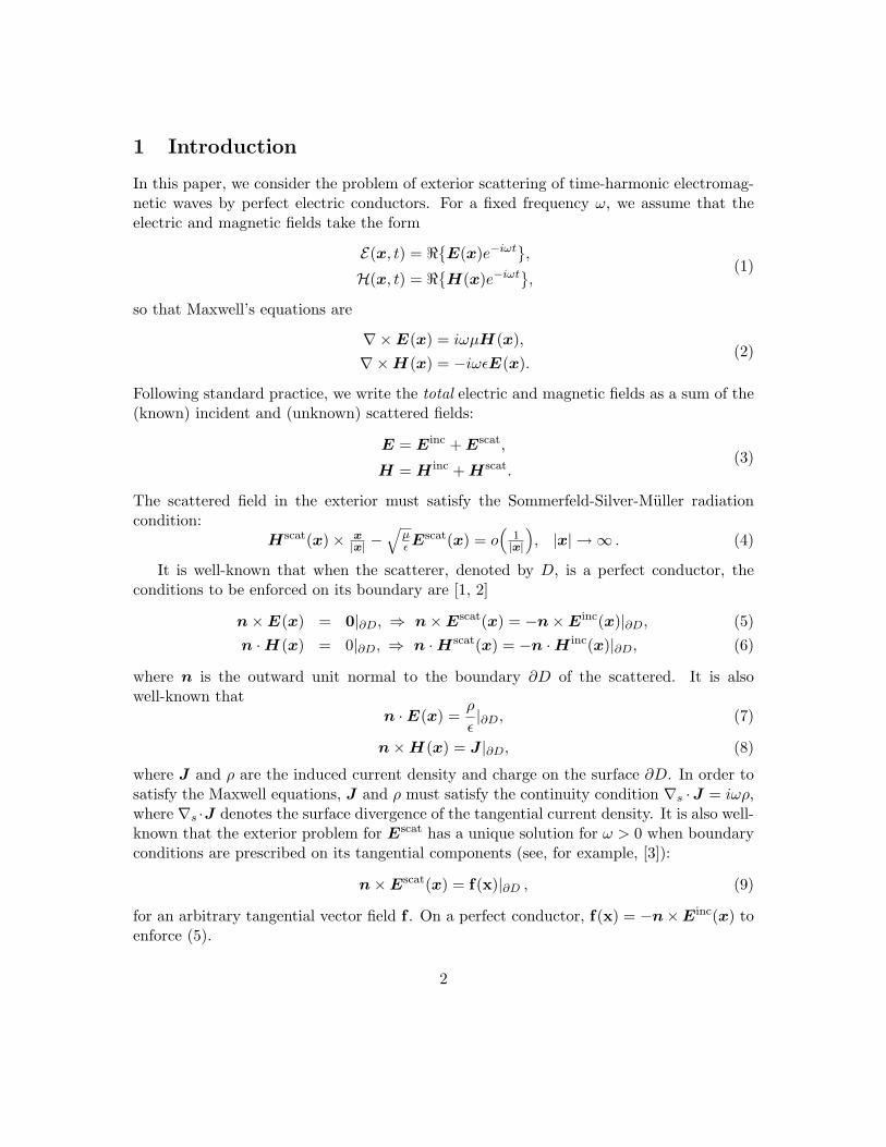
Definition 1. Assuming D is topologically equivalent to a sphere with g handles, one canchoose g surfaces Sj in R3\D so that R3\(D ∪gj=1 Sj) is simply connected. The boundariesof these surfaces are loops on ∂D called B-cycles. They go around the “holes” and form abasis for the first homology group of the domain D.

4

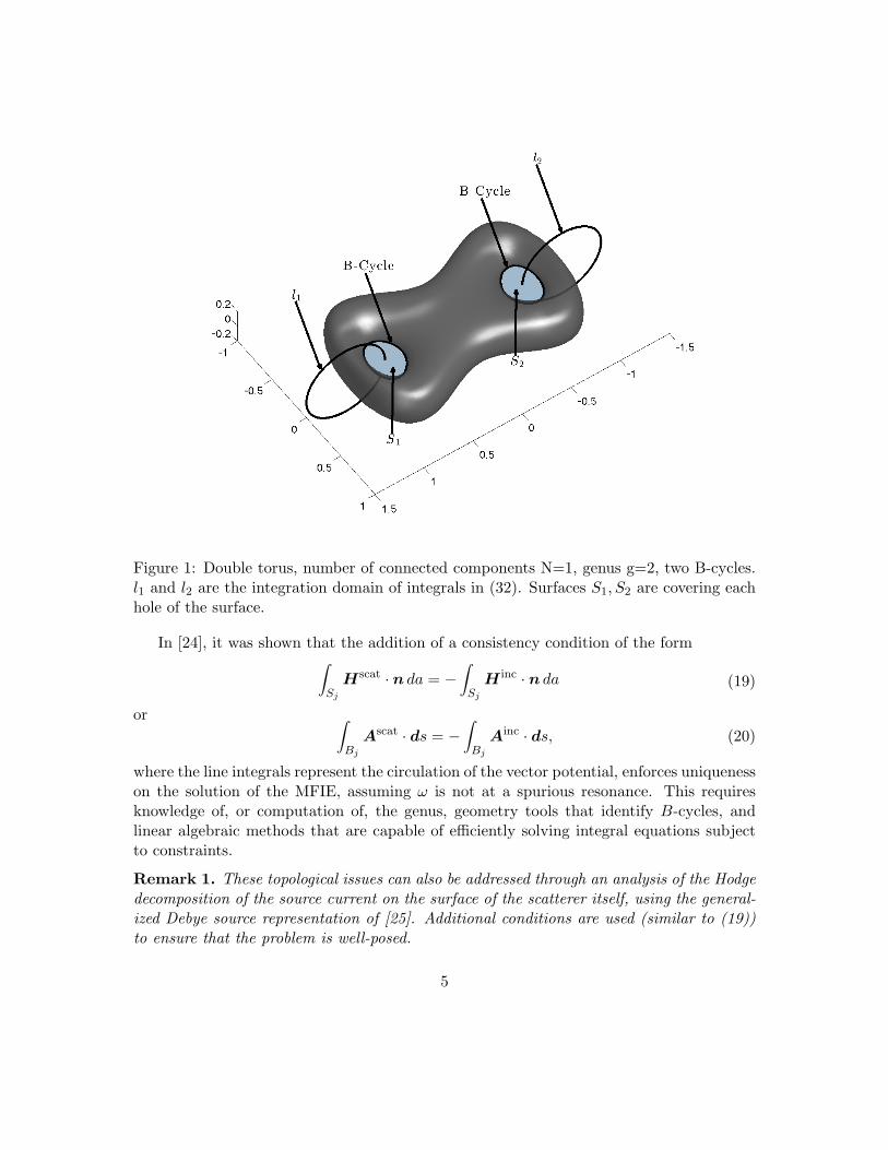
Figure 1: Double torus, number of connected components N=1, genus g=2, two B-cycles.l1 and l2 are the integration domain of integrals in (32). Surfaces S1, S2 are covering eachhole of the surface.

In [24], it was shown that the addition of a consistency condition of the form∫Sj

Hscat · n da = −∫Sj

H inc · n da (19)

or ∫Bj

Ascat · ds = −∫Bj

Ainc · ds, (20)

where the line integrals represent the circulation of the vector potential, enforces uniquenesson the solution of the MFIE, assuming ω is not at a spurious resonance. This requiresknowledge of, or computation of, the genus, geometry tools that identify B-cycles, andlinear algebraic methods that are capable of efficiently solving integral equations subjectto constraints.

Remark 1. These topological issues can also be addressed through an analysis of the Hodgedecomposition of the source current on the surface of the scatterer itself, using the general-ized Debye source representation of [25]. Additional conditions are used (similar to (19))to ensure that the problem is well-posed.

5

Remark 2. Very recently, a method was introduced that overcomes the topological low-frequency breakdown inherent in the EFIE by a clever projection of the discretized problemusing Rao-Wilton-Glisson (RWG) basis functions into a suitable subspace [26].

In short, the various integral equations presently available pose significant difficultiesin the low-frequency regime.

1.2 A decoupled formulation

In this paper we introduce a new formulation for electromagnetic scattering from perfectconductors. Rather than imposing boundary conditions on the field quantities (E, H),we derive conditions on the potentials themselves. Moreover, we show that the integralequations for Ascat and φscat can be decoupled, lead to well-conditioned linear systems,and are insensitive to the genus of the scatterer. More precisely, we seek to impose theboundary conditions

n×Ascat(x) = −n×Ainc(x)|∂D,n×∇φscat(x) = −n×∇φinc(x)|∂D. (21)

At first glance, there is an obvious difficulty with such an approach: the vector andscalar potentials are not unique, a fact generally referred to as gauge freedom. Even in theLorenz gauge above, the representation is known not to be unique. That is, the condition(13) does not completely determine the potentials Ascat, φscat. To see this, consider thevector potentials A′ scat, φ′ scat defined by

A′ scat[J ](x) = Ascat[J ](x) +∇Sk[σ](x),φ′ scat[ρ](x) = φscat[ρ](x) + iωSk[σ](x).

(22)

Here, σ is an arbitrary source on the surface ∂D. It is straightforward to check that thefields Escat,Hscat induced by A′ scat, φ′ scat are the same as those induced by Ascat, φscat,all the while satisfying the Lorenz gauge condition.

We will make use of this additional gauge freedom to establish a well-posed boundaryvalue problem and a stable, well-conditioned integral equation. In Section 2, we considerthe low-frequency limit of the exterior scattering from perfect conductors, both for thesake of review and to motivate our formulation. In Section 3, we discuss the relevantexistence, uniqueness and stability results for what we refer to as the decoupled potentialintegral equation (DPIE). Finally, we discuss the stable representation of the incomingfield in terms of scalar and vector potentials and the high-frequency behavior of the newformulation.

2 Preliminaries

In this section, we consider the low-frequency limit of the Maxwell equations, where theelectric and magnetic fields are decoupled. We will refer to the electrostatic and magneto-

6

static fields by E0 and H0, respectively.

2.1 Electrostatics

The electrostatic field satisfies the equations

∇×E0(x) = 0, ∇ ·E0(x) = 0, x ∈ R3/D, (23)

which we decompose (as above) into incoming and scattered fields. The scattered fieldmust satisfy the radiation condition

Escat0 (x) = o(1), |x| → ∞. (24)

The boundary condition for the electrostatic field is the same as that for any non-zerofrequency,

n×E0(x) = 0, x ∈ ∂D, (25)

but the solution is no longer unique.The nullspace, that is functions satisfying (23) and (25) and the radiation condition

(24), is of dimension N , where N is the number of connected components of the scatterers∂D. They are known as harmonic Dirichlet fields [22] with a basis denoted by {Yj}Nj=1.It is straightforward to see that there are at least N such solutions, since they correspondto the well-studied problem of capacitance. To see this, let us denote by ∂Dj the jthconnected component of ∂D. Taking the static limit of (10), the scattered electrostaticfield is described as the gradient of a scalar harmonic function:

Escat0 = −∇φscat

0 . (26)

Imposing the boundary condition (25) and assuming the incoming field is represented interms of an incoming potential φinc, we have

∆φscat0 = 0,

n×∇φscat0 = −n×∇φinc

0 |∂D.It is clear that the preceding boundary condition is satisfied by any scattered potentialthat satisfies the Dirichlet condition

φscat0 = −φinc

0 |∂Dj+ Vj , (27)

where Vj is an arbitrary constant on ∂Dj that represents the voltage of each conductor(with respect to infinity). The Dirichlet field Yj corresponds to the gradient of φscat

0

obtained by setting φscat0 to zero on each boundary component ∂Di for i 6= j and φscat

0 = 1on ∂Dj . Let us now define the scalars Qj by

Qj =∫∂Dj

∂φscat0

∂nds = −

∫∂Dj

n ·Escat0 ds, (28)

7

so that −Qj is the total charge on each conductor ∂Dj . The matrix that links the voltagesVj and the charges −Qj is known as the capacitance matrix [1]. Since we are interestedhere in the time-harmonic Maxwell equations and their zero-frequency limit, we must havecharge neutrality on each boundary component. Thus, we are interested in studying (27)where the voltages Vj are additional unknowns, but for which N additional constraints aregiven of the form Qj = 0, for j = 1, . . . , N .

It is important to note that, in the static regime, the problem suffers from more thannon-uniqueness. The boundary condition

n×∇φscat0 = −n×Einc

0

cannot be satisfied unless the incoming field is also an electrostatic field. In particular, ifthe circulation of the incoming field

∮L⊂∂D Einc

0 · dl is not zero on every closed loop L onthe surface ∂D, the solution Escat

0 does not exist. This follows easily from the fact that∮L⊂∂D

Einc0 · dl = −

∮L⊂∂D

∇φscat0 · dl = 0.

We refer the reader to [22] for further discussion.

2.2 Magnetostatics

The magnetostatic field satisfies the equations

∇×H0(x) = 0, ∇ ·H0(x) = 0, x ∈ R3/D, (29)

and the boundary conditionn ·H0(x) = 0|∂D. (30)

The total field is again decomposed into incoming and scattered fields, with the scatteredfield satisfying the radiation condition (31),

Hscat0 (x) = o(1), |x| → ∞. (31)

Hscat0 can be described either as the curl of a harmonic vector potential A0 or as the

gradient of a harmonic scalar potential φscat0 .

The magnetostatic problem also suffers from non-uniqueness. The nullspace, that isfunctions satisfying (29) and (30) and the radiation condition (31), is of dimension g, whereg is the genus of the surface ∂D. Elements of this space are called harmonic Neumannfields {Zm}gm=1 [22]. In order to completely specify the solution, additional information,such as the total induced current Im on g loops lying on the surface, must be specified:∮

lmHscat

0 (x) · dl = Im, m = 1, . . . , g . (32)

8

The loops lm here go around the “holes” (see Fig. 1). That is, they are a basis for the firsthomology group of R3\D, with spanning surfaces that lie in the interior of the scatterer,see [22] for more details. The persistent currents Im at zero frequency are due to thepotential presence of superconducting loops (as we are considering scattering from perfectelectric conductors).

2.3 Summary

To summarize, the problem of electromagnetic scattering from perfect conductors is uniquelysolvable for any ω strictly greater than zero. At ω = 0, however, various subtleties arise.The issue of Dirichlet fields needs to be resolved in electrostatics and the issue of Neumannfields needs to be resolved in magnetostatics. For any ω strictly greater than zero, however,it is necessary that the total charge Qj induced on any connected component of the scat-terer be zero. Enforcing this condition at ω = 0 (and introducing the additional unknownconstants Vj as above) uniquely determines the electrostatic field. In the magnetostaticcase, however, we are obligated to introduce additional constants, such as the {Im} in (32),in order to account for the Neumann fields when the scatterer has non-zero genus.

3 Scattering Theory for Decoupled Potentials

We turn now to the analytic foundations of the DPIE. We first derive boundary valueproblems for the scattered scalar and vector potentials that are completely insensitive tothe genus, although they do depend explicitly on the number of boundary components.After this reformulation of the Maxwell equations, we design integral representations thatlead to well-conditioned and invertible linear systems of equations.

Definition 2. By the scalar Dirichlet problem, we mean the calculation of a scalar Helmholtzor Laplace potential in R3\D whose boundary value equals a given function f on ∂D andwhich satisfies standard radiation conditions at infinity:

∆φscat + k2φscat = 0, φscat|∂D = f, (33)

x|x| · ∇φscat(x)− ikφscat(x) = o

(1|x|), |x| → ∞ , (34)

for the scalar Helmholtz potential, and

∆φscat0 = 0, φscat

0 |∂D = f, (35)

φscat0 (x) = O

(1|x|), ∇φscat

0 (x) = O(

1|x|2), |x| → ∞, (36)

for the scalar Laplace potential, respectively.

9

Definition 3. By the vector Dirichlet problem, we mean the calculation of a vectorHelmholtz or Laplace potential in R3\D whose tangential boundary values equal a giventangential function f on ∂D, and whose divergence equals a given scalar function h on ∂Dand which satisfies standard radiation conditions at infinity:

∆Ascat + k2Ascat = 0, n×Ascat|∂D = f , ∇ ·Ascat|∂D = h, (37)

∇×Ascat(x)× x|x| + x

|x|∇ ·Ascat(x)− ikAscat(x) = o(

1|x|), |x| → ∞ , (38)

for the vector Helmholtz potential, and

∆Ascat0 = 0, n×Ascat

0 |∂D = f , ∇ ·Ascat0 |∂D = h, (39)

Ascat0 (x) = O

(1|x|), ∇×Ascat

0 (x) = O(

1|x|2), ∇ ·Ascat

0 (x) = O(

1|x|2), |x| → ∞ ,

(40)for the vector Laplace potential, respectively.

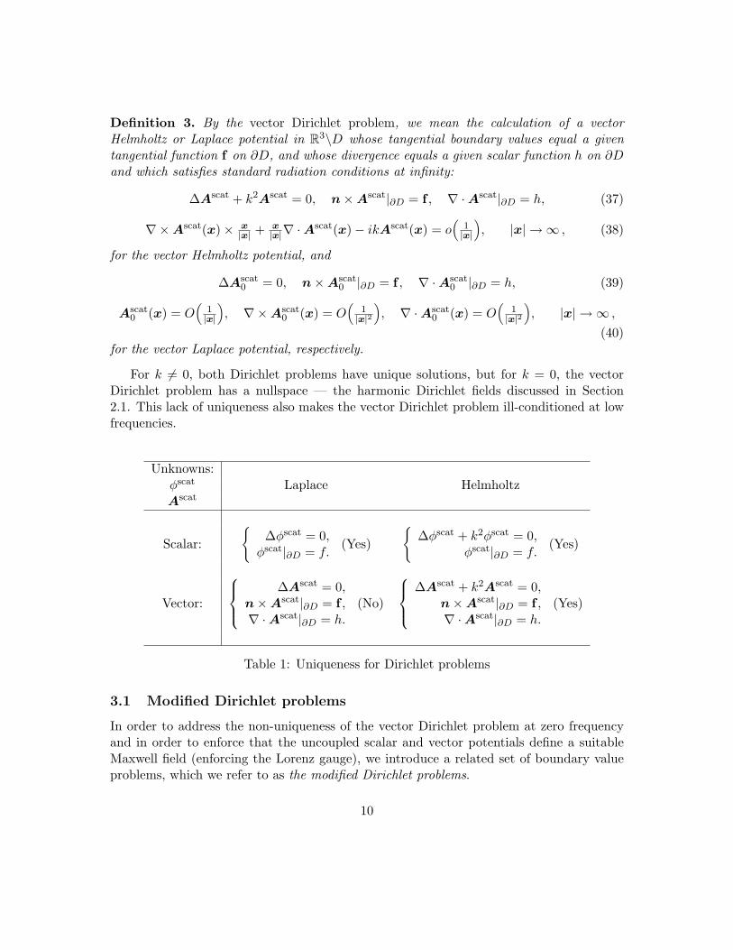
For k 6= 0, both Dirichlet problems have unique solutions, but for k = 0, the vectorDirichlet problem has a nullspace — the harmonic Dirichlet fields discussed in Section2.1. This lack of uniqueness also makes the vector Dirichlet problem ill-conditioned at lowfrequencies.

Unknowns:φscat Laplace HelmholtzAscat

Scalar:

{∆φscat = 0,φscat|∂D = f.

(Yes)

{∆φscat + k2φscat = 0,

φscat|∂D = f.(Yes)

Vector:

∆Ascat = 0,

n×Ascat|∂D = f ,∇ ·Ascat|∂D = h.

(No)

∆Ascat + k2Ascat = 0,

n×Ascat|∂D = f ,∇ ·Ascat|∂D = h.

(Yes)

Table 1: Uniqueness for Dirichlet problems

3.1 Modified Dirichlet problems

In order to address the non-uniqueness of the vector Dirichlet problem at zero frequencyand in order to enforce that the uncoupled scalar and vector potentials define a suitableMaxwell field (enforcing the Lorenz gauge), we introduce a related set of boundary valueproblems, which we refer to as the modified Dirichlet problems.

10

Definition 4. By the scalar modified Dirichlet problem, we mean the calculation of ascalar Helmholtz or Laplace potential in R3\D which satisfies standard radiation condi-tions at infinity. Letting N denote the number of connected components of the boundary∂D, we introduce extra unknown degrees of freedom {Vj}Nj=1 and the boundary data f issupplemented with additional (known) constants {Qj}Nj=1. For the scalar Helmholtz poten-tial,

∆φscat + k2φscat = 0, φscat|∂Dj= f + Vj , (41)

x|x| · ∇φscat(x)− ikφscat(x) = o

(1|x|), |x| → ∞ , (42)

with ∫∂Dj

∂φscat

∂nds = Qj .

For the scalar Laplace potential,

∆φscat0 = 0, φscat

0 |∂Dj= f + Vj , (43)

φscat0 (x) = O

(1|x|), ∇φscat

0 (x) = O(

1|x|2), |x| → ∞, (44)

with ∫∂Dj

∂φscat

∂nds = Qj .

Definition 5. By the vector modified Dirichlet problem, we mean the calculation of a vec-tor Helmholtz or Laplace potential in R3\D which satisfies standard radiation conditions atinfinity. Letting N denote the number of connected components of the boundary ∂D, we in-troduce extra unknown degrees of freedom {vj}Nj=1 and the boundary data f is supplementedwith additional (known) constants {qj}Nj=1. For the vector Helmholtz potential,

∆Ascat + k2Ascat = 0, n×Ascat|∂D = f , ∇ ·Ascat|∂Dj= h+ vj , (45)

∇×Ascat(x)× x|x| + x

|x|∇ ·Ascat(x)− ikAscat(x) = o(

1|x|), |x| → ∞ , (46)

with ∫∂Dj

n ·Ascatds = qj .

For the vector Laplace potential,

∆Ascat0 = 0, n×Ascat

0 |∂D = f , ∇ ·Ascat0 |∂Dj

= h+ vj , (47)

Ascat0 (x) = O

(1|x|), ∇×Ascat

0 (x) = O(

1|x|2), ∇ ·Ascat

0 (x) = O(

1|x|2), |x| → ∞ ,

(48)with ∫

∂Dj

n ·Ascatds = qj .

11

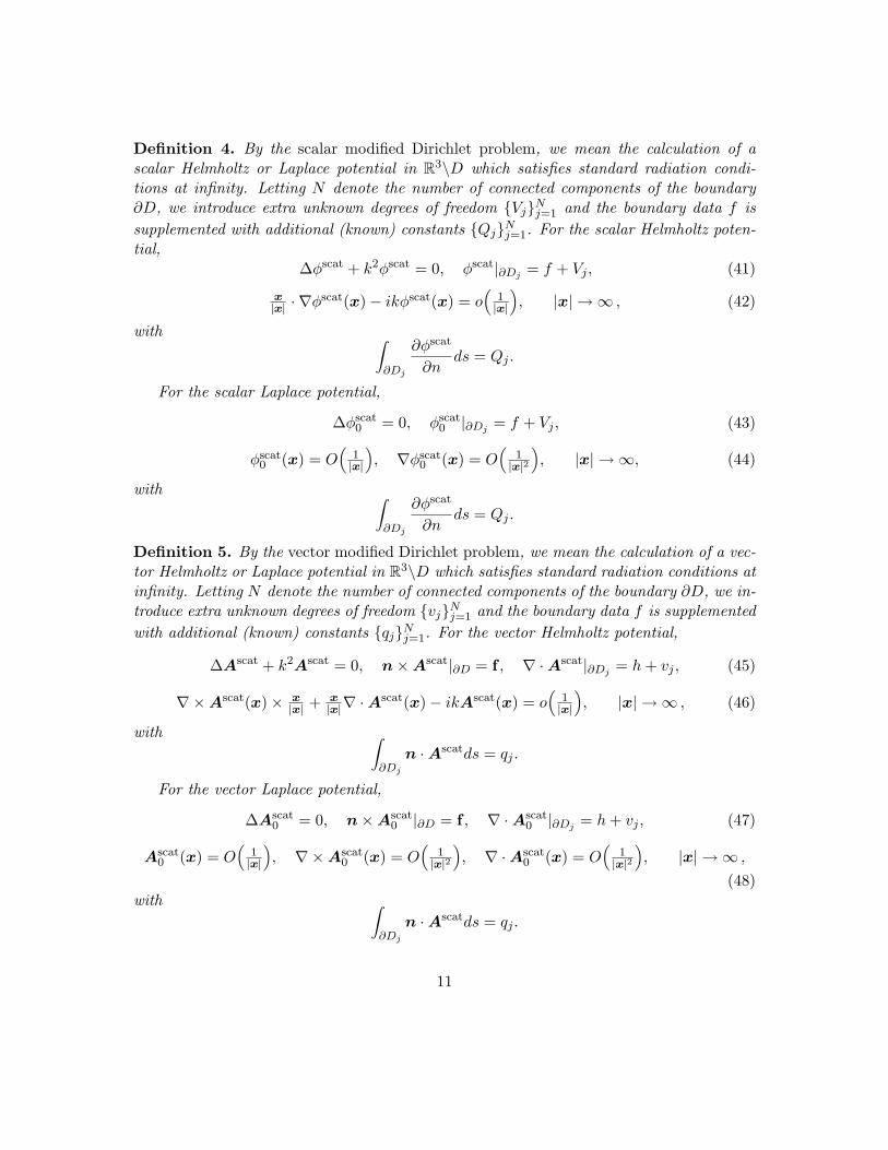
We summarize the modified Dirichlet boundary value problems in Table 2.

Unknowns:φscat, {Vj}Nj=1 Laplace HelmholtzAscat, {vj}Nj=1

Scalar:

∆φscat = 0,

φscat|∂Dj= f + Vj ,∫

∂Dj

∂φscat

∂n ds = Qj .

(Yes)

∆φscat + k2φscat = 0,φscat|∂Dj

= f + Vj ,∫∂Dj

∂φscat

∂n ds = Qj .

(Yes)

Vector:

∆Ascat = 0,

n×Ascat|∂D = f ,∇ ·Ascat|∂Dj

= h+ vj ,∫∂Dj

n ·Ascatds = qj .

(Yes)

∆Ascat + k2Ascat = 0,

n×Ascat|∂D = f ,∇ ·Ascat|∂Dj

= h+ vj ,∫∂Dj

n ·Ascatds = qj .

(Yes)

Table 2: Uniqueness for modified Dirichlet problems

We now define the scattered scalar and vector potentials in terms of modified Dirichletproblems.

Definition 6. Let φinc,Ainc denote incoming scalar and vector potentials and assume thatD is a perfect conductor. The scattered scalar potential φscat is the solution to the scalarmodified Dirichlet problem with boundary data:

f := −φinc|∂Dj, Qj := − ∫∂Dj

φinc

∂n ds . (49)

Likewise, the scattered vector potential Ascat is the solution to the vector modified Dirichletproblem with boundary data:

f := −n×Ainc|∂D, h := −∇ ·Ainc|∂D, qj := − ∫∂Djn ·Aincds . (50)

3.2 Uniqueness

We begin with two well-known theorems from scattering theory.

Theorem 1. [22] Let φscat be a scalar Helmholtz potential with wavenumber k, (k 6= 0) inthe exterior domain R3\D, satisfying the radiation condition (34) and the condition

Is = ={k

∫∂D

φscat∂φscat

∂nds

}≥ 0. (51)

Here, ={f} denotes the imaginary part of f . Then, φscat = 0 in R3\D.

12

Theorem 2. [22] Let Ascat be a vector Helmholtz potential with wavenumber k, (k 6= 0)in the exterior domain R3\D, satisfying the radiation condition (38) and the condition

Iv = ={k

∫∂D

n×Ascat · ∇ ×Ascat + n ·Ascat∇ ·Ascat

ds

}≥ 0 . (52)

Then, Ascat = 0 in R3\D.

We now show that the modified Dirichlet problems have unique solutions in all regimes.For simplicity, we assume that k is real. The proofs are analogous when the wavenumberk has a positive imaginary part, which adds dissipation.

Theorem 3. The scalar modified Dirichlet problem has at most one solution for any k > 0.

Proof. Consider a solution of the homogeneous problem (f = 0, Qj = 0):∆φscat + k2φscat = 0,φscat|∂D = 0 + Vj ,∫∂Dj

∂φscat

∂n ds = 0.(53)

The quantity Is in (51) is then given by

Is = ={k

∫∂D

φscat∂φscat

∂nds

}= =

{k

N∑j=1

Vj

∫∂Dj

∂φscat

∂n

}= 0. (54)

Thus, by Theorem 1, φscat = 0 and using the boundary condition φscat|∂Dj= 0 + Vj , we

get Vj = 0.

Theorem 4. The vector modified Dirichlet problem has at most one solution for any k > 0.

Proof. Consider a solution of the homogeneous problem (f = 0, h = 0, qj = 0):∆Ascat + k2Ascat = 0,

n×Ascat|∂D = 0,∇ ·Ascat|∂Dj

= 0 + vj ,∫∂Dj

n ·Ascatds = 0.

(55)

The quantity Iv in 52 is then given by

Iv = ={k

∫∂D

n×Ascat · ∇ ×Ascat + n ·Ascat∇ ·Ascat

ds

}=

= ={k

N∑j=1

vj

∫∂Dj

n ·Ascatds

}= 0.

(56)

Thus, by Theorem 2, Ascat = 0 and using the boundary condition ∇ ·Ascat|∂Dj= 0 + vj ,

we obtain vj = 0.

13

Theorem 5. The scalar modified Dirichlet problem for the Laplace equation has at mostone solution.

Proof. This is a well-known result. When f = 0, the relation between Qj and Vj is thecapacitance matrix [1] and this matrix is always invertible (Theorem 5.6 in [22]). Thus, ifQj = 0, then Vj = 0. The fact that φscat = 0 follows from the maximum principle [27].

Before proving the uniqueness of the vector modified Dirichlet problem for the Laplaceequation we need the following technical result that shows a relation between the vectorand scalar modified Dirichlet problems. This Lemma will also be used in section 4 to provethe connection between electromagnetic scattering and modified Dirichlet problems.

Lemma 1. Let Ascat, {vj}Nj=1 be a solution of the vector modified Dirichlet problem withboundary data f , h, {qj}Nj=1 for (k ≥ 0). Then,

ψscat := ∇ ·Ascat, {Vj = vj}Nj=1 (57)

satisfies the scalar modified Dirichlet problem with boundary data:

f := h, {Qj = −k2qj}Nj=1 . (58)

Proof. By hypothesis, Ascat satisfies

∆Ascat + k2Ascat = 0 (59)

n×Ascat|∂D = f (60)

∇ ·Ascat|∂Dj= h+ vj (61)∫

∂Dj

n ·Ascatds = qj . (62)

Taking the divergence of (59), we get

∆∇ ·Ascat + k2∇ ·Ascat = 0 . (63)

Therefore, ψscat = ∇ ·Ascat satisfies the Helmholtz equation. From 61, we get

ψscat = ∇ ·Ascat = h+ vj |∂Dj. (64)

Finally, we may write

∇×∇×Ascat = k2Ascat +∇∇ ·Ascat ⇒n · ∇ ×∇×Ascat = k2n ·Ascat + n · ∇∇ ·Ascat ⇒

−∇s · (n×∇×Ascat) = k2n ·Ascat + n · ∇∂ψscat

∂n⇒

−∫∂Dj

∇s · (n×∇×Ascat)ds = 0 = k2∫∂Dj

n ·Ascatds+∫∂Dj

∂ψscat

∂nds .

(65)

14

Using the boundary condition (62), we obtain∫∂Dj

∂ψscat

∂nds = −k2qj , (66)

and the result follows.

Theorem 6. The vector modified Dirichlet problem for the Laplace equation has at mostone solution.

Proof. Let (Ascat, vj) be a solution of the homogeneous vector modified Dirichlet problem.Then, applying Lemma 1, (∇ · Ascat, {vj}Nj=1) satisfies the homogeneous scalar modifiedDirichlet problem By Theorem 5, ψscat = ∇·Ascat = 0 and vj = 0. By theorem 5.9 in [22],Ascat is a harmonic Dirichlet field, and thus a linear combination of the basis functions{Yj}Nj=1. It follows from the flux conditions

∫∂Dj

n ·Ascatds = 0 that Ascat = 0.

3.3 Existence and stability

In this section, we use the Fredholm alternative to obtain existence results for the modifiedDirichlet problems, making use of the single and double layer potentials, Sk and Dk, ofclassical potential theory. We also show that the solution depends continuously on theboundary data, uniformly in k in a neighborhood of k = 0. Next we define classicaloperators in potential theory:

Skσ =∫∂D

gk(x− y)σ(y)dAy,

Dkσ =∫∂D

∂gk∂ny

(x− y)σ(y)dAy,

S′kσ =∫∂D

∂gk∂nx

(x− y)σ(y)dAy,

D′kσ =∂

∂nx

∫∂D

∂gk∂ny

(x− y)σ(y)dAy,

(67)

where x ∈ ∂D and the Green’s function on the free space is:

gk(x) =eik|x|

4π|x| . (68)

For off-surface evaluations x ∈ R3\∂D we have:

Sk[σ](x) =∫∂D

gk(x− y)σ(y)dAy,

Dk[σ](x) =∫∂D

∂gk∂ny

(x− y)σ(y)dAy.(69)

15

Theorem 7. Suppose that we represent the solution to the scalar modified Dirichlet problemwith k > 0 in the form

φscat(x) = Dk[σ](x)− iηSk[σ](x) , (70)

with η ∈ R\{0}. Then, imposing the desired boundary conditions and constraints leads toa Fredholm equation of the second kind:

σ

2+Dkσ − iηSkσ −

N∑j=1

Vjχj = f,

∫∂Dj

(D′kσ + iη

σ

2− iηS′kσ

)ds = Qj ,

(71)

where χj denotes the characteristic function for boundary ∂Dj. Here, σ and the constants{Vj}Nj=1 are unknowns. Moreover, (71) is invertible and the result holds for the modifiedDirichlet problem governed by the Laplace equation (k = 0) as well.

Proof. See Appendix A.

In order to study the vector modified Dirichlet problem, we define the following dyadicoperators:

L

(aρ

)=

(L11a + L12ρL21a + L22ρ

), (72)

whereL11a = n× Ska,L12ρ = − n× Sk(nρ),L21a = 0,L22ρ = Dkρ,

(73)

and

R

(aρ

)=

(R11a +R12ρR21a +R22ρ

), (74)

whereR11a = n× Sk(n× a),R12ρ = n×∇Sk(ρ),R21a = ∇ · Sk(n× a),

R22ρ = − k2Skρ.

(75)

Theorem 8. Suppose that we represent the solution to the vector modified Dirichlet problemwith k > 0 in the form

Ascat = ∇× Sk[a](x)− Sk[nρ](x) + iη(Sk[n× a](x) +∇Sk[ρ](x)

), (76)

16

with η ∈ R\{0}. Then, for |η| sufficiently small, imposing the desired boundary conditionsand constraints leads to a Fredholm equation of the second kind:

12

(aρ

)+ L

(aρ

)+ iηR

(aρ

)+

(0∑N

j=1 vjχj

)=

(fh

),∫

∂Dj

(n · ∇ × Ska− n · Sk(nρ) + iη

(n · Sk(n× a)− ρ

2+ S′kρ

))ds = qj ,

(77)

where χj denotes the characteristic function for boundary ∂Dj. Here, a, ρ and the constants{vj}Nj=1 are unknowns. Moreover, (77) is invertible and the result holds for the vectormodified Dirichlet problem governed by the vector Laplace equation (k = 0) as well.

Proof. See Appendix A.

Definition 7. We will refer to (71) and (77) as the scalar and vector decoupled potentialintegral equations. The former will be abbreviated by DPIEs and the latter by DPIEv.Together, they form the DPIE.

The following two theorems show that the solutions to the modified Dirichlet problemsare continuous functions of the boundary data all the way to k = 0. In particular, they areindependent of the genus of ∂D.

Theorem 9. The scalar modified Dirichlet problem has a unique solution for k ≥ 0.Moreover, the solution depends continuously on the boundary data f, {Qj}Nj=1 in the sensethat the operator mapping the given boundary data onto the solution is uniformly continuousfrom

f, {Qj}Nj=1 ∈ C0,α(∂D)× CN → φscat, {Vj}Nj=1 ∈ C0,α(R3/D)× CN

for any k ∈ [0, kmax], with fixed kmax. C0,α(X) here is equipped with the usual Holder norm[22].

Proof. See Appendix A.

Theorem 10. The vector modified Dirichlet problem has a unique solution for k ≥ 0.Moreover, the solution depends continuously on the boundary data f , h, {qj}Nj=1 in the sensethat the operator mapping the given boundary data onto the solution is uniformly continuousfrom

f , h, {Qj}Nj=1 ∈ T 0,α(∂D)× C0,α(∂D)× CN → Ascat, {vj}Nj=1 ∈ C0,α(R3/D)× CN

for any k ∈ [0, kmax], with fixed kmax. Here, T 0,α(∂D) is equipped with the usual Holdernorm [22].

Proof. See Appendix A.

17

4 Electromagnetic scattering and modified Dirichlet prob-lems

In this section, we explain the connection between the scalar and vector modified Dirichletproblems and the Maxwell equations. It is evident from Theorems 9 and 10 that, if sucha reformulation exists, then we have overcome the topological low-frequency breakdownthat makes electromagnetic scattering from surfaces with nontrivial genus so difficult atlow frequency.

We will first show that the vector and scalar modified Dirichlet problems preserve theLorenz gauge, so that the induced E and H fields are Maxwellian. We will also showthat the calculation is stable, in the sense that bounded “incoming” data leads to bounded“outgoing” data, independent of the frequency. We will then show, in Theorem 12, that themodified Dirichlet problems lead directly to the solution of the desired scattering problem.

Theorem 11. Let Ainc, φinc be bounded (for ω → 0) incoming vector and scalar Helmholtzpotentials in the Lorenz gauge:

∇ ·Ainc = iωµεφinc . (78)

Then, the associated vector and scalar scattered Helmholtz potentials Ascat, φscat (see Def-inition 6) are also bounded and satisfy the Lorenz gauge condition.

Proof. By Lemma 1, the scalar Helmholtz potential ψscat = ∇ ·Ascat satisfies

ψscat = h+ vj = −∇ ·Ainc + vj∣∣∂D∫

∂Dj

∂ψscat

∂nds = −k2qj = k2

∫∂Dj

n ·Aincds .(79)

Using the Lorenz gauge condition on the boundary itself, we may write

ψscat = h+ vj = −iωµεφinc + vj∣∣∂D

. (80)

Since∇ · (iωAinc −∇φinc) = 0 , (81)

we have ∫∂Dj

∂φinc

∂nds = iω

∫∂Dj

n ·Aincds . (82)

Thus,∫∂Dj

∂ψscat

∂nds = k2

∫∂Dj

n ·Aincds =k2

iω

∫∂Dj

∂φinc

∂nds = −iωµε

∫∂Dj

∂φinc

∂nds . (83)

18

From (80) and (83), we see that ψscat and iωµεφscat satisfy the same scalar modifiedDirichlet problem. By uniqueness (Theorem 3), we find that

iωµεφscat = ψscat = ∇ ·Ascat ,

so that Ascat and φscat are in the Lorenz gauge. By Theorems 9 and 10, Ascat, φscat areuniformly continuous functions of Ainc, φinc for k ∈ [0, kmax]. Since Ainc, φinc are bounded,Ascat, φscat are also bounded.

The next theorem is the main result of the present paper.

Theorem 12. For any k ≥ 0, let Einc,Hinc be an incoming electromagnetic field describedby the potentials Ainc, φinc in the Lorenz gauge:

H inc =1µ∇×Ainc,

Einc = iωAinc −∇φinc,

∇ ·Ainc = iωµεφinc ,

and let Ascat, φscat denote the corresponding scattered vector and scalar potentials (Defini-tion 6). Then the electromagnetic fields Escat,Hscat scattered from a perfect conductor aregiven by

Hscat =1µ∇×Ascat,

Escat = iωAscat −∇φscat.

with∇ ·Ascat = iωµεφscat,

n×Escat = −n×Einc|∂D, n ·Hscat = −n ·H inc|∂D.Proof. Since Ascat, φscat are Helmholtz potentials in the Lorenz gauge, the associatedEscat,Hscat are valid Maxwell fields that satisfy the necessary radiation condition. Weneed only check that the desired boundary conditions are satisfied. From the boundaryconditions on Ascat, φscat we have

n×Ascat = −n×Ainc|∂D⇒ iωn×Ascat = −iωn×Ainc|∂D ,

(84)

φscat = −φinc + Vj |∂Dj

⇒ n×∇φscat = −n×∇φinc|∂D .(85)

Adding (84) and (85), we have

iωn×Ascat − n×∇φscat = −iωn×Ainc + n×∇φinc|∂D⇒ n×Escat = −n×Einc|∂D .

(86)

19

Taking the surface divergence of (84), we also have that

n×Ascat = −n×Ainc|∂D⇒ ∇s · n×Ascat = −∇s · n×Ainc|∂D

⇒ n ·Hscat = −n ·H inc|∂D .(87)

Thus, for k > 0 we have the correct solution. While continuity arguments are sufficientto verify that the zero frequency solution is the desired one, it is worth checking that thenet charge still vanishes at k = 0 and that the consistency conditions (19) are satisfied.For this, note first that A, φ are bounded, so that at k = 0,

H inc0 = lim

k→0H inc = ∇×Ainc

0 ,

Einc0 = lim

k→0Einc = −∇φinc

0 ,

Hscat0 = lim

k→0Hscat = ∇×Ascat

0 ,

Escat0 = lim

k→0Escat = −∇φscat

0 .

(88)

The net charge is computed as the surface integral of n ·E, and we have∫∂Dj

n ·Escat0 ds = −

∫∂Dj

∂φscat0

∂nds =

∫∂Dj

∂φinc0

∂nds =

∫Dj

∆φinc0 dv = 0,∫

∂Dj

n ·Escatds =∫∂Dj

iωn ·Ascat − ∂φscat

∂nds =

= −∫∂Dj

iωn ·Ainc − ∂φinc

∂nds =

∫Dj

∇ · (iωAinc −∇φinc)dv = 0 .

(89)

The last equality follows from the fact that the incoming potentials are assumed to bespecified in the Lorenz gauge. In short,∫

∂Dj

n ·Escat0 ds = lim

k→0

∫∂Dj

n ·Escatds = 0 , (90)

as expected. The consistency conditions (19) on the flux of the magnetic field through eachhole Sj [24] are also easily verified for all ω ≥ 0:

n×Ascat = −n×Ainc|∂D⇒∮Bj

Ascat · dl = −∮Bj

Ainc · dl . (91)

Here, Bj is a B-cycle, namely a loop on ∂D which goes around some “hole” and whosespanning surface Sj lies in the exterior of the domain (see Figure 1 and related discussion).

20

5 Incoming Potentials

In a stable DPIE approach, the vector and scalar potentials must be defined in the Lorenzgauge and be bounded as ω → 0. We will need to find a representation for the incomingfields that will permit the stable uncoupling of the vector and scalar potentials. Assumingwe are given the “impressed” free current and charge J imp, ρimp, the incoming potentials

Ainc(x) = µSk[J imp](x),

φinc(x) =1εSk[ρimp](x),

(92)

satisfy these requirements. For an incoming plane wave with a polarization vector Ep anda direction of propagation u, given by

Einc = Epeiku·x, H inc = Hpe

iku·x =u×Ep

Zeiku·x, (93)

where Z =√

µε , the standard representation of incoming vector and scalar potentials

Ainc =1iω

Einc, φinc = 0, (94)

does not lead to stable uncoupling, since the vector potential is unbounded, as ω → 0.But, as mentioned above, the Lorenz gauge does not, by itself, impose uniqueness on thegoverning potentials. It is easy to check that the vector and scalar potentials defined by

A′ inc = −u(x ·Ep)√µεeiku·x,

φ′ inc = −x ·Epeiku·x,

(95)

satisfy the Lorenz gauge condition

∇ ·A′ inc(x) = iωµεφ′ inc(x), (96)

both A′ inc and φ′ inc are bounded Helmholtz potentials, as ω → 0, and represent the sameincoming plane wave (93). See Appendix B for more details how to stably decomposeincoming/outgoing electric and magnetic multipole fields (Debye sources).

6 The DPIE and the Aharonov-Bohm effect

In classical physics, the Maxwell equations are described in terms of the components ofthe electric and magnetic fields, with the vector and scalar potentials viewed as matters ofcomputational convenience. In quantum mechanics, however, it was shown by Aharonovand Bohm [28] that an electron is sensitive to the vector potential A itself, in regions whereE and H are identically zero (the Aharonov-Bohm effect).

21

Let us first recall that the two pairs of potentials {A, φ} and {A′, φ′} produce the sameelectromagnetic field, so long as they satisfy the condition

A′ = A +∇ψ,φ′ = φ+ iωψ .

(97)

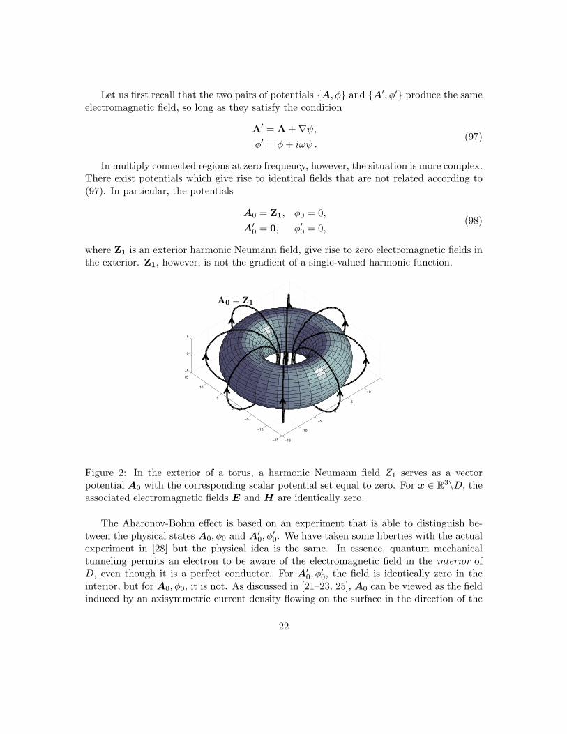
In multiply connected regions at zero frequency, however, the situation is more complex.There exist potentials which give rise to identical fields that are not related according to(97). In particular, the potentials

A0 = Z1, φ0 = 0,A′0 = 0, φ′0 = 0,

(98)

where Z1 is an exterior harmonic Neumann field, give rise to zero electromagnetic fields inthe exterior. Z1, however, is not the gradient of a single-valued harmonic function.

−15

−10

−5

0

5

10

15

−15

−10

−5

0

5

10

15

−5

0

5

A0scat = Ascat +r scat

�0scat = �scat + ik scat (102)

In a multiply connected region, the reciprocal is not true. Next example illustrates it:

−15

−10

−5

0

5

10

15

−15

−10

−5

0

5

10

15

−5

0

5

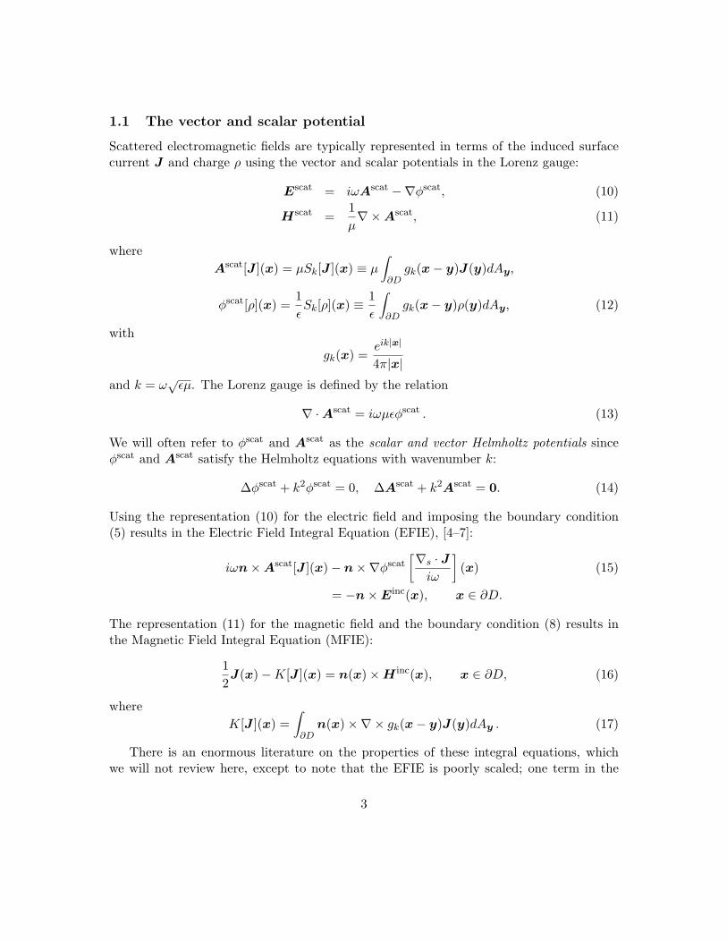
Figure 5: Vector potential A0 = Z1 in the exterior region x 2 R3\D corresponding to anexterior Neumann mode. The associated fields are E,H = 0

Consider the potentials for k = 0:

A0 = Z1, �0 = 0A0

0 = 0, �00 = 0

(103)

Both potentials produce the same field Etot,Htot = 0 as r ⇥ A0 = 0, nevertheless,both potentials are not equivalent in the sense of 102 as Z0 is a Neumann mode. Aquantum physical experiment designed by Aharonov and Bohm in [?] allows to distinguishbetween the physical state A,� and A0,�0. A relationship between the DPIE approachthat we propose and the Aharonov-Bohm e↵ect appears. Given that our approach dealswith vector and scalar potentials directly, it can also distinguish between the state A,�and A0,�0.

Considere the vector and scalar potentials scattering problem with boundary conditions:

n⇥A0|@D = n⇥ Z1, r · A0|@D = 0, �0|@D = 0n⇥A0

0|@D = 0, r · A00|@D = 0, �0

0|@D = 0(104)

22

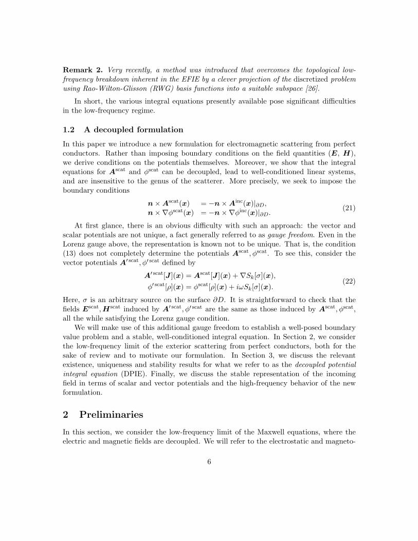
Figure 2: In the exterior of a torus, a harmonic Neumann field Z1 serves as a vectorpotential A0 with the corresponding scalar potential set equal to zero. For x ∈ R3\D, theassociated electromagnetic fields E and H are identically zero.

The Aharonov-Bohm effect is based on an experiment that is able to distinguish be-tween the physical states A0, φ0 and A′0, φ′0. We have taken some liberties with the actualexperiment in [28] but the physical idea is the same. In essence, quantum mechanicaltunneling permits an electron to be aware of the electromagnetic field in the interior ofD, even though it is a perfect conductor. For A′0, φ′0, the field is identically zero in theinterior, but for A0, φ0, it is not. As discussed in [21–23, 25], A0 can be viewed as the fieldinduced by an axisymmetric current density flowing on the surface in the direction of the

22

arrows in Fig. 2. This induces a non-trivial magnetic field within the torus. Electrons, asa result, sense whether they traveled through the hole of the torus or passed by the toruson the outside. The DPIE formalism easily distinguishes between these two cases, since wedeal with the vector and scalar potentials directly. Thus, A0, φ0,A

′0 and φ′0 in (98) satisfy

n×A0|∂D = n× Z1, ∇ ·A0|∂D = 0, φ0|∂D = 0,n×A′0|∂D = 0, ∇ ·A′0|∂D = 0, φ′0|∂D = 0 .

(99)

7 The DPIE in the high frequency regime

Theorems 7 and 8 suggest that the numerical solution of scattering problems in the presenceof perfect conductors can be effectively solved through the use of the DPIE, defined byequations (71) and (77). The scalar part of these equations (71) is a Fredholm equation ofthe second kind, invertible for all frequencies. As stated in Theorem 8, however, the vectorpart (77) is a Fredholm equation only for sufficiently small coupling constant |η| < ‖R‖−1.The difficulty is that the operator R is continuous and bounded, but not compact. Infact, its spectrum has three cluster points: λ = 0.5, λ = 0.5 + i0.5 and λ = 0.5− i0.5 (see[29, 30]). While the uniqueness proof holds for arbitrary values of η, existence requiresfurther analysis. We suspect that the vector part of DPIE is invertible for all frequenciesand leave the formal result as a conjecture. In fact, numerical experiments suggest thatη should not be chosen too small when seeking to optimize the condition number of theDPIE.

Our interest in the DPIE formulation grew out of issues in low-frequency scattering.Nevertheless, we would like to find a representation that is effective at all frequencies, andthis will involve a slight rescaling of the equations. In order to carry out a suitable analysis,we follow [31] and study scattering from the unit sphere ∂D = {x : ‖x‖ = 1}. For k ≤ 1,setting η = 1 works well, while for k > 1 the optimal scaling factor η ≈ k (see [31]). Settingη = k, instead of (71), we have the scaled DPIEs integral equation:

σ

2+Dkσ − ikSkσ −

N∑j=1

Vjχj = f,

∫∂Dj

(1kD′kσ + i

σ

2− iS′kσ

)ds =

1kQj ,

(100)

where the second set of equations has been multiplied by a factor of 1k . For the vector

modified Dirichlet problem, when k > 1, we replace (76) with

Ascat = ∇× Sk[a](x)− kSk[n%](x) + i(kSk[n× a](x) +∇Sk[%](x)

), (101)

where we have multiplied the single-layer potential terms by k, and set η = 1. We alsorescale the boundary condition∇·Ascat = −∇·Ascat+vn in the modified Dirichlet problem,

23

dividing each side by k. These changes lead to the scaled DPIEv integral equation:

12

(aρ

)+ Ls

(aρ

)+ iRs

(aρ

)+

(0∑N

j=1 vjχj

)=

(f1kh

),∫

∂Dj

(n · ∇ × Ska− kn · Sk(n%) + i

(kn · Sk(n× a)− %

2+ S′k%

))ds = qj ,

(102)

where

Ls =

(L11 kL121kL21 L22

), Rs =

(kR11 R12

R211kR22

), (103)

with Lij , Rij defined in (73).We turn now to the analysis of the DPIE on the unit sphere, where exact expressions

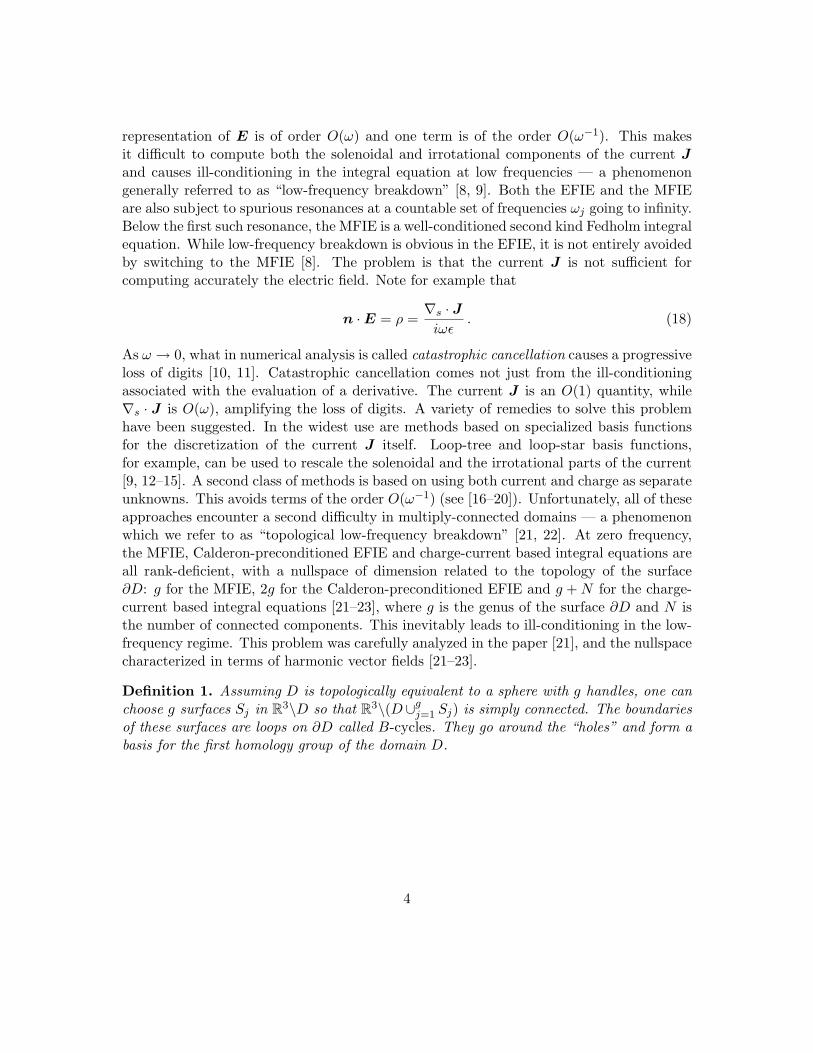
for the various integral operators have been worked out in detail [32]. More precisely, usingscalar and vector spherical harmonics, each integral operator has a simple signature, whichhas been tabulated in [32]. This permits us to compute the condition number and spectrumof the DPIEs and DPIEv integral equations. In Figs. 3 and 4, we plot the spectrum andthe singular values of the scaled DPIEv (102).

0 0.5 1 1.5 2 2.5 3−3

−2

−1

0

1

Real

Imag

Eigenvalues DPIE

Figure 3: Spectrum of the scaled DPIEv integral equation (102) for a spherical scattererof radius 1 at k = 10. As discussed in the text, there are three different cluster points: atλ = 0.5, λ = 0.5 + i0.5 and λ = 0.5− i0.5.

24

0 20 40 60 80 1000

1

2

3

4

5

n (singular value index)

Sing

ular

val

ue

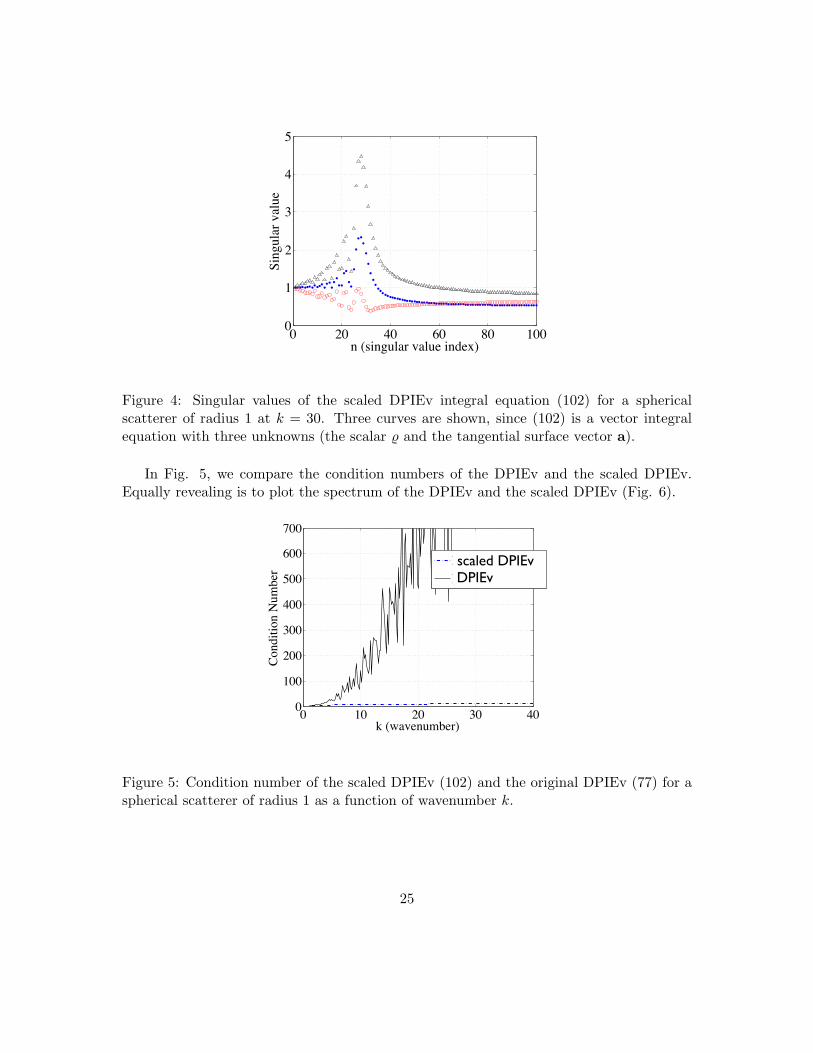
Figure 4: Singular values of the scaled DPIEv integral equation (102) for a sphericalscatterer of radius 1 at k = 30. Three curves are shown, since (102) is a vector integralequation with three unknowns (the scalar % and the tangential surface vector a).

In Fig. 5, we compare the condition numbers of the DPIEv and the scaled DPIEv.Equally revealing is to plot the spectrum of the DPIEv and the scaled DPIEv (Fig. 6).

0 10 20 30 400

100

200

300

400

500

600

700

k (wavenumber)

Con

ditio

n N

umbe

r

DPIE NormalizedDPIE

scaled DPIEv DPIEv

Sunday, December 8, 13

Figure 5: Condition number of the scaled DPIEv (102) and the original DPIEv (77) for aspherical scatterer of radius 1 as a function of wavenumber k.

25

0 20 40 60 80−60

−40

−20

0

20

40

Real

Imag

Eig. DPIEEig. DPIE normalizedEig. of DPIEv

Eig. of scaled DPIEv

Sunday, December 8, 13

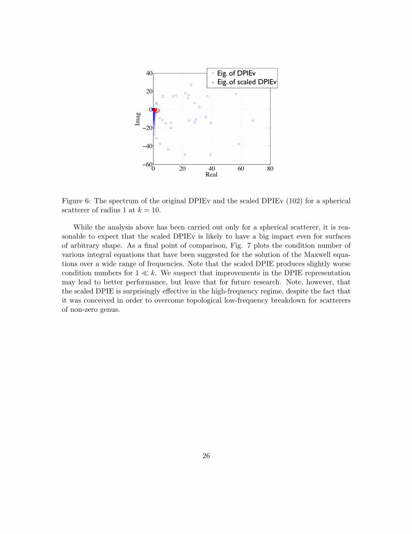
Figure 6: The spectrum of the original DPIEv and the scaled DPIEv (102) for a sphericalscatterer of radius 1 at k = 10.

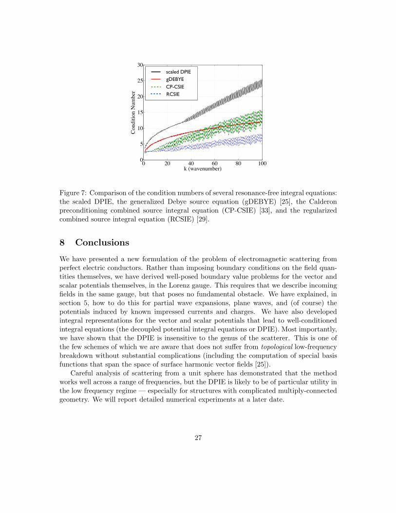
While the analysis above has been carried out only for a spherical scatterer, it is rea-sonable to expect that the scaled DPIEv is likely to have a big impact even for surfacesof arbitrary shape. As a final point of comparison, Fig. 7 plots the condition number ofvarious integral equations that have been suggested for the solution of the Maxwell equa-tions over a wide range of frequencies. Note that the scaled DPIE produces slightly worsecondition numbers for 1 � k. We suspect that improvements in the DPIE representationmay lead to better performance, but leave that for future research. Note, however, thatthe scaled DPIE is surprisingly effective in the high-frequency regime, despite the fact thatit was conceived in order to overcome topological low-frequency breakdown for scatterersof non-zero genus.

26

0 20 40 60 80 1000

5

10

15

20

25

30

k (wavenumber)

Con

ditio

n N

umbe

r

gDEBYECP−CFIEDPIE NormalizedRCSIE

scaled DPIEgDEBYE

CP-CSIERCSIE

Friday, December 6, 13

Figure 7: Comparison of the condition numbers of several resonance-free integral equations:the scaled DPIE, the generalized Debye source equation (gDEBYE) [25], the Calderonpreconditioning combined source integral equation (CP-CSIE) [33], and the regularizedcombined source integral equation (RCSIE) [29].

8 Conclusions

We have presented a new formulation of the problem of electromagnetic scattering fromperfect electric conductors. Rather than imposing boundary conditions on the field quan-tities themselves, we have derived well-posed boundary value problems for the vector andscalar potentials themselves, in the Lorenz gauge. This requires that we describe incomingfields in the same gauge, but that poses no fundamental obstacle. We have explained, insection 5, how to do this for partial wave expansions, plane waves, and (of course) thepotentials induced by known impressed currents and charges. We have also developedintegral representations for the vector and scalar potentials that lead to well-conditionedintegral equations (the decoupled potential integral equations or DPIE). Most importantly,we have shown that the DPIE is insensitive to the genus of the scatterer. This is one ofthe few schemes of which we are aware that does not suffer from topological low-frequencybreakdown without substantial complications (including the computation of special basisfunctions that span the space of surface harmonic vector fields [25]).

Careful analysis of scattering from a unit sphere has demonstrated that the methodworks well across a range of frequencies, but the DPIE is likely to be of particular utility inthe low frequency regime — especially for structures with complicated multiply-connectedgeometry. We will report detailed numerical experiments at a later date.

27

Acknowledgements

This work was supported in part by the Applied Mathematical Sciences Program of theU.S. Department of Energy under Contract DEFGO288ER25053 (L.G.) and by the Officeof the Assistant Secretary of Defense for Research and Engineering and AFOSR underNSSEFF Program Award FA9550-10-1-0180 (L.G. and Z. G.) and in part by the SpanishMinistry of Science and Innovation (Ministerio de Ciencia e Innovacion) under the projectsCSD2008-00068 and TEC2010-20841-C04-01. The authors thank A. Klockner and M.ONeil for many useful discussions.

A Proofs of existence and stability theorems

Proof of Theorem 7:Consider a solution σ, {Vj}Nj=1 of the homogeneous equation (71):

σ

2+Dkσ − iηSkσ −

N∑j=1

Vjχj = 0,

∫∂Dj

(D′kσ + iη

σ

2− iηS′kσ

)ds = 0 .

(104)

For this solution, the scalar function and constants

φscat(x) = Dk[σ](x)− iηSk[σ](x), {Vj}Nj=1 (105)

satisfy the scalar modified Dirichlet problem with right-hand side f = 0, {Qj = 0}Nj=1. ByTheorem 3, we have φscat = 0, {Vj = 0}Nj=1. As φscat is represented by a combination ofsingle and double layers, it is known that σ = 0. This proves uniqueness (see [3, 22]). Notethat the operators Dk and Sk defined on C0,α(∂D) are compact (see [22]). The rest ofthe operators in (71) are finite rank, so that (100) is a second kind equation when actingon the space C0,α(∂D) × CN , where CN is equipped with the usual finite-dimensionaltopology. Note also that, as a function of k, the operators involved are continuous in therange k ∈ [0, kmax] for any fixed kmax. This implies that the operators involved in equation(71) are not only compact, but collectively compact as well (see [34, 35]). By the Fredholmtheorem, for any right hand side f, {Qj}Nj=1 ∈ C0,α(∂D) × CN , there exists a solutionσ, {Vj}Nj=1 ∈ C0,α(∂D)× CN .

Proof of Theorem 8:

28

Consider a solution a, %, {vj}Nj=1 of the homogeneous equation (106):

12

(a%

)+ L

(a%

)+ iηR

(a%

)−(

0∑Nj=1 vjχj

)=

(00

),∫

∂Dj

(n · ∇ × Ska− n · Sk(n%) + iη

(n · Sk(n× a)− %

2+ S′kV0%

))ds = 0 .

(106)

For this solution, the vector field and constants

Ascat = ∇× Sk[a](x)− Sk[n%](x) + iη(Sk[n× a](x) +∇Sk[%](x)

), {vj}Nj=1 (107)

satisfy the vector modified Dirichlet problem, with right hand side f = 0, h = 0, {qj =0}Nj=1. By Theorem 4, we have Ascat = 0, {Vj = 0}Nj=1. It is known that a zero fieldAscat = 0 with this representation (107) must have trivial sources (see [22]). Thus, a = 0and % = 0, which proves uniqueness (see [3]).

Note that the operator L defined on T 0,α(∂D)×C0,α(∂D) is compact (see Table [22]).The operator R is continuous and bounded on T 0,α(∂D) × C0,α(∂D), but not compact.However, for a choice of the constant |η| < ‖R‖−1, I + iηR has a bounded inverse givenby its Neumann series. The rest of the operators in equation (106) are finite rank, sothat equation (106) is second kind when acting on the space T 0,α(∂D)× C0,α(∂D)× CN ,where CN is equipped with the usual finite-dimensional topology. Note also that, as afunction of k, the operators involved are continuous in the range k ∈ [0, kmax] for anyfixed kmax. This implies that the operators involved in equation 106 are not only compact,but collectively compact as well (see [34]). By Fredholm theory, for any right hand sidef , h, {qj}Nj=1 ∈ T 0,α(∂D)×C0,α(∂D)×CN , there exists a solution a, %, {vj}Nj=1 ∈ T 0,α(∂D)×C0,α(∂D)× CN .

Proof of Theorem 9:The solution of the integral equation (71) depends continuously on the right hand sidef, {Qj}Nj=1, with the corresponding Holder topology. Due to the collective compactnessof the operators involved in (71), the continuity is uniform in k ∈ [0, kmax]. The mapφscat(σ, {Vj}Nj=1) is continuous on C0,α(∂D) × CN → C0,α(R3\D) × CN (see [22]). Bycomposition, the map φscat(f, {Qj}Nj=1) is continuous as a map from C0,α(∂D) × CN →C0,α(R3\D)× CN , uniformly on k ∈ [0, kmax]. That is,

‖φscat‖0,α,R3\D ≤ K(α,∂D,kmax)

(‖f‖0,α,∂D +

N∑j=1

|Qj |2), (108)

where the constant K(α,∂D,kmax) depends on α, the surface ∂D, and the maximum frequencykmax. The result is valid uniformly down to zero frequency k = 0.

29

Proof of Theorem 10:The solution of (77) depends continuously on the right hand side with the correspondingHolder topology. Due to the collective compactness of the operators involved in (77), thecontinuity is uniform in k ∈ [0, kmax]. The map Ascat(a, %, {vj}Nj=1) : T 0,α(∂D)×C0,α(∂D)×CN → T 0,α(R3\D)×C0,α(R3\D)×CN is continuous (see [22]). By composition, the mapAscat(f , h, {qj}Nj=1) : T 0,α(∂D) × C0,α(∂D) × CN → T 0,α(R3\D) × C0,α(R3\D) × CN iscontinuous, uniformly in k for k ∈ [0, kmax]. That is,

‖Ascat‖0,α,R3\D ≤ K(α,∂D,kmax)

(‖f‖0,α,∂D + ‖h‖0,α,∂D +

N∑j=1

|qj |2), (109)

where the constant K(α,∂D,kmax) depends on α, the surface ∂D and the maximum frequencykmax. The result is valid uniformly down to zero frequency k = 0.

B Partial wave expansions

An important representation of the electromagnetic field is that based on separation ofvariables in spherical coordinates. As shown independently by Lorenz, Debye and Mie[2, 25], the fields induced by sources in the interior of a sphere can always be expressed inthe exterior of the sphere according to the representation:

Efar =∑m,n

[amn∇×∇× (xhn(k|x|)Y m

n ) + iωµbmn∇× (xfn(k|x|)Y mn )],

Hfar =∑m,n

[bmn∇×∇× (xhn(k|x|)Y m

n )− iωεamn∇× (xfn(k|x|)Y mn )],

(110)

where hn is the spherical Hankel function of the first kind. For sources in the exterior ofthe sphere, we have

Eloc =∑m,n

[amn∇×∇× (xjn(k|x|)Y m

n ) + iωµbmn∇× (xfn(k|x|)Y mn )],

H loc =∑m,n

[bmn∇×∇× (xjn(k|x|)Y m

n )− iωεamn∇× (xfn(k|x|)Y mn )],

(111)

where jn is the spherical Bessel function [36]. In order to obtain a finite static limit, werenormalize and define the modified spherical Hankel/Bessel function by

fn(k, r) :=

{hn(k, r) = hn(kr) kn+1

−i(2n−1)(2n−3)...5·3·1 ,jn(k, r) = jn(kr) (2n+1)(2n−1)...5·3·1

kn+1 .(112)

It is easy to check that

limk→0

fn(k, r) =

{limk→0 hn(k, r) = 1

rn+1 ,

limk→0 jn(k, r) = rn.(113)

30

With a slight abuse of notation we will refer to both Efar and Eloc as Einc, and toboth Hfar and H loc as H inc. When the distinction is important, we will specify the useof hn(k, r) or jn(k, r) as the radial function of interest.

Normalizing the coefficients amn, bmn by the inverse of the scaling factor in (112), wewrite:

Einc =∑m,n

[amn∇×∇× (xfn(k, |x|)Y m

n ) + iωµbmn∇× (xfn(k, |x|)Y mn )],

H inc =∑m,n

[bmn∇×∇× (xfn(k, |x|)Y m

n )− iωεamn∇× (xfn(k, |x|)Y mn )].

(114)

The fields of a magnetic multipole of degree n and order m are defined to be

Eincnm = iωµ∇× (xfn(k, |x|)Y m

n ),

Hincnm = ∇×∇× (xfn(k, |x|)Y m

n ) .(115)

The corresponding vector and scalar potentials can be defined by

Aincnm = µ∇× (xfn(k, |x|)Y m

n ),

φincnm = 0 .

(116)

They clearly satisfy∆φinc

nm + k2φincnm = 0,

∆Aincnm + k2A

incnm = 0,

∇ · Aincnm = iωµεφinc

nm .

(117)

Moreover, Aincmn and φinc

mn are bounded. The fields of an electric multipole of degree n andorder m are defined to be

Eincnm = ∇×∇× (xfn(k, |x|)Y m

n ),

Hincnm = −iωε∇× (xfn(k, |x|)Y m

n ) .(118)

In this case, however, it is easy to verify that the function which serves as the obviousvector potential, namely xfn(k, |x|)Y m

n , is not in the Lorenz gauge. To find a suitablereplacement, we compute:

∇×∇× (xfn(k, |x|)Y mn ) = k2xfn(k, |x|)Y m

n +∇ ∂

∂r

(rfn(k, r)Y m

n

)r=|x| . (119)

Note that∂

∂r

(rfn(k, r)Y m

n

)= fn(k, r)Y m

n + r∂

∂rfn(k, r)Y m

n . (120)

31

The first term fn(k, r)Y mn is a Helmholtz potential. Making use of the following identity

for spherical Hankel and Bessel functions [36]

n+ 1z

hn(z) + h′n(z) = hn−1(z),n

zjn(z)− j′n(z) = jn+1(z),

(121)

we have

r∂

∂rhn(k, r) =

rk2

2n− 1hn−1(k, r)− (n+ 1)hn(k, r) (122)

and

r∂

∂rjn(k, r) = − rk2

2n+ 3jn+1(k, r) + njn(k, r) . (123)

Multiplying by Y mn ,

r∂

∂rhn(k, r)Y m

n =rk2

2n− 1hn−1(k, r)Y m

n − (n+ 1)hn(k, r)Y mn ,

r∂

∂rjn(k, r)Y m

n = − rk2

2n+ 3jn+1(k, r)Y m

n + njn(k, r)Y mn .

(124)

The first term on the right-hand side is of the order O(k), while the second term is aHelmholtz potential and of magnitude O(1). Using (124) and (120) in (119), we obtain

∇×∇× (xhn(k, |x|)Y mn ) = k2xhn(k, |x|)Y m

n +k2

2n− 1∇(rhn−1(k, r)Y m

n

)r=|x|

−∇(nhn(k, r)Y mn

)r=|x| ,

(125)

for the outgoing waves, and

∇×∇× (xjn(k, |x|)Y mn ) = k2xjn(k, |x|)Y m

n −k2

2n+ 3∇(rjn+1(k, r)Y m

n

)r=|x|

+∇((n+ 1)jn(k, r)Y mn

)r=|x| ,

(126)

for the incoming waves. Note that the last term on the right-hand side of (126) and theleft-hand side of (126) both satisfy the vector Helmholtz equation. Thus, the first two termson the right-hand side of (126) must together satisfy the vector Helmholtz equation as well.Dividing those two terms by k2 and multiplying by −iωµε, we define the correspondingvector and scalar potentials by

Aincnm = −iωµεxhn(k, |x|)Y m

n +−iωµε2n− 1

∇(rhn−1(k, r)Y mn

)r=|x|,

φincnm = nhn(k, |x|)Y m

n ,

(127)

32

for the outgoing waves, and

Aincnm = −iωµεxjn(k, |x|)Y m

n +iωµε

2n+ 3∇(rjn−1(k, r)Y m

n

)r=|x|,

φincnm = −(n+ 1)jn(k, |x|)Y m

n ,

(128)

for the incoming waves. It is easy to verify that

∆φincnm + k2φinc

nm = 0,

∆Aincnm + k2A

incnm = 0,

∇ · Aincnm = iωµεφinc

nm .

(129)

The last equation, which enforces the Lorenz gauge, is obtained by taking the divergenceof (126). Clearly, both potentials A

incmn and φinc

mn are of the order O(1).

33

References

[1] J. D. Jackson. Classical Electrodynamics. John Wiley & Sons: New York, 1975.

[2] Charles Herach Papas. Theory of electromagnetic wave propagation. Courier DoverPublications, 1988.

[3] David Lem Colton and Rainer Kress. Inverse acoustic and electromagnetic scatteringtheory, volume 93. Springer, 2013.

[4] Weng Cho Chew. Waves and fields in inhomogenous media. IEEE press New York,1995.

[5] Jian-Ming Jin. Theory and computation of electromagnetic fields. Wiley. com, 2011.

[6] Jin-Fa Lee, Robert Lee, and Robert J Burkholder. On the formulation of a generalscattering problem by means of an integral equation. Z. Phys, 126:610–618, 1949.

[7] Claus Muller. Foundations of the mathematical theory of electromagnetic waves.Springer Berlin, 1969.

[8] Yunhua Zhang, Tie Jun Cui, Weng Cho Chew, and Jun-Sheng Zhao. Magnetic fieldintegral equation at very low frequencies. IEEE Transactions on Antennas and Prop-agation, 51(8):1864–1871, 2003.

[9] Jun-Sheng Zhao and Weng Cho Chew. Integral equation solution of Maxwell’s equa-tions from zero frequency to microwave frequencies. IEEE Transactions on Antennasand Propagation, 48(10):1635–1645, 2000.

[10] Rainer Kress. On the limiting behaviour of solutions to boundary integral equationsassociated with time harmonic wave equations for small frequencies. MathematicalMethods in the Applied Sciences, 1(1):89–100, 1979.

[11] Rainer Kress. A singular perturbation problem for linear operators with an applicationto the limiting behavior of stationary electromagnetic wave fields for small frequencies.Meth. Verf. Math. Phys., 21:5–30, 1981.

[12] Jin-Fa Lee, Robert Lee, and Robert J Burkholder. Loop star basis functions and arobust preconditioner for EFIE scattering problems. IEEE Transactions on Antennasand Propagation, 51(8):1855–1863, 2003.

[13] Giuseppe Vecchi. Loop-star decomposition of basis functions in the discretization ofthe EFIE. IEEE Transactions on Antennas and Propagation, 47(2):339–346, 1999.

[14] DR Wilton and AW Glisson. On improving the electric field integral equation at lowfrequencies. Proc. URSI Radio Sci. Meet. Dig, page 24, 1981.

34

[15] Wen-Liang Wu, Allen W Glisson, and Darko Kajfez. A study of two numerical so-lution procedures for the electric field integral equation at low frequency. AppliedComputational Electromagnetics Society Journal, 10(3):69–80, 1995.

[16] Matti Taskinen and Pasi Yla-Oijala. Current and charge integral equation formulation.IEEE Transactions on Antennas and Propagation, 54(1):58–67, 2006.

[17] Matti Taskinen and Simopekka Vanska. Current and charge integral equation formu-lations and Picard’s extended Maxwell system. IEEE Transactions on Antennas andPropagation, 55(12):3495–3503, 2007.

[18] Felipe Vico, Zydrunas Gimbutas, Leslie Greengard, and Miguel Ferrando-Bataller.Overcoming low-frequency breakdown of the magnetic field integral equation. IEEEtransactions on Antennas and Propagation, 61(3):1285–1290, 2013.

[19] P Yla-Oijala, Matti Taskinen, and S Jarvenpaa. Advanced surface integral equationmethods in computational electromagnetics. In Electromagnetics in Advanced Appli-cations, 2009. ICEAA’09. International Conference on, pages 369–372. IEEE, 2009.

[20] A. Bendali, F. Collino, M. Fares, and B. Steif. Extension to nonconforming meshes ofthe combined current and charge integral equation. IEEE Transactions on Antennasand Propagation, 60(10):4732–4744, 2012.

[21] Kristof Cools, Francesco P Andriulli, Femke Olyslager, and Eric Michielssen.Nullspaces of MFIE and Calderon preconditioned EFIE operators applied to toroidalsurfaces. IEEE Transactions on Antennas and Propagation, 57(10):3205–3215, 2009.

[22] David L Colton and Rainer Kress. Integral equation methods in scattering theory,volume 57. Wiley New York, 1983.

[23] Peter Werner. On an integral equation in electromagnetic diffraction theory. Journalof Mathematical Analysis and Applications, 14(3):445–462, 1966.

[24] Charles L Epstein, Zydrunas Gimbutas, Leslie Greengard, Andreas Klockner, andMichael O’Neil. A consistency condition for the vector potential in multiply-connecteddomains. IEEE Transactions on Magnetics, 49(3):1072–1076, 2013.

[25] Charles L Epstein and Leslie Greengard. Debye sources and the numerical solution ofthe time harmonic Maxwell equations. Communications on Pure and Applied Mathe-matics, 63(4):413–463, 2010.

[26] Francesco P Andriulli, Kristof Cools, and Eric Michielssen. On a well-conditionedelectric field integral operator for multiply connected geometries. IEEE Transactionson Antennas and Propagation, 61(4):2077–2087, 2013.

35

[27] Lawrence C. Evans. Partial Differential Equations. American Mathematical Society,Providence, RI, 1998.

[28] Yakir Aharonov and David Bohm. Significance of electromagnetic potentials in thequantum theory. Physical Review, 115(3):485, 1959.

[29] Oscar Bruno, Tim Elling, Randy Paffenroth, and Catalin Turc. Electromagnetic in-tegral equations requiring small numbers of Krylov-subspace iterations. Journal ofComputational Physics, 228(17):6169–6183, 2009.

[30] Jean-Claude Nedelec. Acoustic and electromagnetic equations: Integral representationsfor harmonic problems, volume 144. Springer, 2001.

[31] Rainer Kress. Minimizing the condition number of boundary integral operators inacoustic and electromagnetic scattering. The Quarterly Journal of Mechanics andApplied Mathematics, 38(2):323–341, 1985.

[32] Felipe Vico, Zydrunas Gimbutas, and Leslie Greengard. Boundary integral equationanalysis on the sphere. Numer. Math, to appear, 2014.

[33] H. Contopanagos, B. Dembart, M. Epton, J.J. Ottusch, V. Rokhlin, J.L. Visher,and S.M. Wandzura. Well-conditioned boundary integral equations for three-dimensional electromagnetic scattering. IEEE Transactions on Antennas and Propa-gation, 50(12):1824–1830, 2002.

[34] P. M. Anselone. Uniform approximation theory for integral equations with discontin-uous kernels. SIAM Journal on Numerical Analysis, 4(2):245–253, 1967.

[35] Kendall E Atkinson. The numerical solution of integral equations of the second kind.Cambridge University Press, 1997.

[36] Milton Abramowitz and Irene A Stegun. Handbook of Mathematical Functions: WithFormulars, Graphs, and Mathematical Tables, volume 55. Dover Publications, 1964.

36